Assessment of the impact of ethanol content in gasoline on fuel consumption, including a literature review up to 2006

The oil companies’ European association for Environment, Health and Safety in refining and distribution

report no. 13/13

conservation of clean air and water in europe © CONCAWE

report no. 13/13

I

Assessment of the impact of ethanol content in gasoline on fuel consumption, including a literature review up to 2006 Prepared for the CONCAWE Fuels Quality and Emissions Management Group by its Special Task Force FE/STF-20: R. Stradling (Chair) A. Bellier M.O. Del Rio Barrio J.H. Farenback-Brateman H. Hovius A. Jackson A. Joedicke U. Kiiski S. Maroto de Hoyos W. Mirabella C. Olivares Molina K. Skaardalsmo J. Williams P.J. Zemroch (Consultant) D.J. Rickeard (Consultant) K.D. Rose (Science Executive) N.D. Thompson (Technical Coordinator) Reproduction permitted with due acknowledgement CONCAWE Brussels December 2013

report no. 13/13

II

ABSTRACT

Ethanol, at low concentrations in motor gasoline, is known to impact both the fuel consumption and emissions from vehicles. Because ethanol has a lower energy content per litre compared to conventional hydrocarbon gasoline, a vehicle’s volumetric fuel consumption generally increases when running on ethanol/gasoline blends. In principle, factors such as the higher octane number and high latent heat of vaporisation for ethanol could allow better engine efficiency which could mitigate this effect to some extent. The degree to which modern vehicles can compensate for the lower energy content of ethanol compared to conventional gasoline is not reliably known, however. This is an important question because it impacts the interpretation of Well-to-Wheels results for biofuel blends used in conventional vehicles. For this reason, an assessment of published literature up to 2006 was completed in order to evaluate the impact of ethanol content on fuel consumption.

The scope of this literature assessment was on the use of low-level ethanol/gasoline blends, specifically 5% (E5) and 10% (E10) v/v ethanol in gasoline. These blends are the most common ethanol levels in Europe today and have been formalised in the CEN EN 228 standard for motor gasoline. This literature review did not evaluate the impact of other oxygenate types that are also allowed in the EN 228 standard.

Although many publications were evaluated, the number of studies containing relevant data was limited primarily because the experimental variability in fuel consumption results was relatively large. From this analysis, the following conclusions could be made from the evaluated publications:

There is a relatively high incidence of incorrectly derived fuel consumption data, usually resulting in an underestimate of the increase in fuel consumption from ethanol-containing gasolines.

For some studies on gasoline blends containing up to E20, the increase in mass fuel consumption (FC) was typically only about 50% of the expected value, based on simply the loss in calorific value from ethanol addition. In the most extreme case, fuels with almost identical energy contents showed a fuel consumption difference of more than 4%, although for the majority of vehicles, the difference was generally less than 2%. For the largest data set (7 vehicles using up to 10 test fuels), the overall trend showed a 3.97% increase in fuel consumption with a 3.4% reduction in fuel energy content.

It is not clear that this variation in FC results was related to variations in fuel parameters other than the ethanol content. Rather, it is assumed that the variability in FC was primarily a consequence of experimental variation and poorly controlled test procedures. The variability found in these published studies limits the firm conclusions that can be drawn about the influence of low levels of ethanol on vehicle fuel consumption.

These conclusions suggested that a more definitive vehicle study was warranted to determine whether modern vehicles can or cannot compensate for the lower energy content of ethanol-containing gasoline through better engine efficiency. Such a study has now been completed by the JEC1 Consortium and is reported elsewhere [5].

1 Three organisations comprise the JEC Consortium: the Joint Research Centre (JRC) of the European

Commission, the European Council for Automotive R&D (EUCAR), and CONCAWE

report no. 13/13

III

KEYWORDS

Ethanol, motor gasoline, petrol, fuel consumption, EN 228

INTERNET

This report is available as an Adobe pdf file on the CONCAWE website (www.concawe.org).

NOTE Considerable efforts have been made to assure the accuracy and reliability of the information contained in this publication. However, neither CONCAWE nor any company participating in CONCAWE can accept liability for any loss, damage or injury whatsoever resulting from the use of this information. This report does not necessarily represent the views of any company participating in CONCAWE.

report no. 13/13

IV

CONTENTS Page

SUMMARY V 

1.  INTRODUCTION 1 

2.  THEORETICAL EFFECTS 2 2.1.  INTRODUCTION 2 2.2.  TYPICAL PROPERTIES 2 2.3.  THEORETICAL EFFECTS OF LATENT HEAT AND

THROTTLING 5 2.3.1.  The effect of airflow and throttling 6 2.3.2.  Effect of latent heat of vaporisation (1) 7 2.3.3.  The effect of latent heat (2) 8 2.4.  EPA FUEL CONSUMPTION CORRECTION 10 

3.  LITERATURE ASSESSMENT 11 3.1.  INFORMATION ON FUEL CONSUMPTION 11 3.2.  FINAL FUEL CONSUMPTION DATA 11 

4.  CONCAWE DATA 14 4.1.  JEC EVAPORATIVE EMISSIONS PROGRAMME 14 4.2.  CONCAWE GASOLINE EMISSIONS PROGRAMME 15 

5.  CONCLUSIONS 17 

6.  GLOSSARY 19 

7.  ACKNOWLEDGMENTS 20 

8.  REFERENCES 21 

APPENDIX 1  RELEVANT PUBLICATIONS ON FUEL CONSUMPTION THROUGH 2006 22 

APPENDIX 2  CARBON BALANCE FUEL CONSUMPTION 30 A2.1.  BASIC EQUATION 30 A2.2.  EPA GASOLINE EQUATION 31 

APPENDIX 3  RESULTS FROM CONCAWE TEST PROGRAMMES 35 A3.1.  JEC EVAPORATIVE EMISSIONS PROGRAMME 35 A3.2.  CONCAWE GASOLINE EMISSIONS PROGRAMME 38 

report no. 13/13

V

SUMMARY

Ethanol, at low concentrations in motor gasoline, is known to impact both the fuel consumption and emissions from vehicles. Because ethanol has a lower energy content per litre compared to conventional hydrocarbon gasoline, volumetric fuel consumption (FC) generally increases when running on ethanol/gasoline blends. In principle, factors such as the higher octane number and high latent heat of ethanol could allow better engine efficiency, which could also mitigate this effect to some extent. The degree to which modern vehicles can compensate for the lower energy content of ethanol is not reliably known, however. This is an important question because it impacts the interpretation of Well-to-Wheels results for biofuel blends and conventional vehicles. For this reason, an assessment of published literature up to 2006 was completed in order to evaluate the impact of ethanol content in gasoline on FC.

The scope of this assessment was on the use of low-level ethanol/gasoline blends, specifically 5% (E5) and 10% (E10) v/v ethanol in gasoline. These blends are the most common ethanol levels in Europe today and have been formalised in the CEN EN 228 standard for motor gasoline. This literature review did not evaluate the impact of other oxygenate types that are also allowed in the EN 228 standard.

A literature review, completed on references up to 20062, identified approximately 25 studies for more detailed analysis that were considered to be most relevant on the impact of ethanol in gasoline on vehicle FC. Although some studies included information on much higher ethanol concentrations, such as E85 and E95, vehicle modifications would be required at these ethanol contents and the impact of FC alone could be confounded by hardware changes. For this reason, this literature assessment is limited to low-level ethanol blends in motor gasoline.

Although many studies were evaluated, the final set of relevant data was very limited. It was also evident from the available data that the degree of variability in FC results was relatively large. Thus non-ethanol data sets were also examined to evaluate the variability in FC that can typically be expected from vehicle testing programmes.

From the analysis of the available literature data, the following conclusions could be made:

There is a relatively high incidence of incorrectly derived FC data, usually resulting in an underestimate of the FC from ethanol-containing gasolines. In some cases, this was due to the use of an unadjusted carbon weight fraction in the carbon-balance equation. In other cases, the gasoline equation from the US Environmental Protection Agency (EPA) was used that attempts to correct for differences in fuel calorific value.

For some studies on gasoline blends containing up to 20% v/v ethanol (E20), the measured increase in mass FC was typically only about 50% of the expected value, based on simply the loss in calorific value when a certain volume of ethanol was added. For example, with an E10 blend, a 2% mass FC increase was measured compared to the 4% mass FC that was expected.

2 This literature review was completed several years ago in order to complement the development of

specifications for low-level ethanol/gasoline blends that were in progress at the time.

report no. 13/13

VI

In the most extreme case, fuels with almost identical energy contents showed a fuel consumption difference of more than 4%, although for the majority of vehicles, the difference was generally less than 2%.

For the largest data set (7 vehicles using up to 10 test fuels), the overall trend showed a 3.97% increase in fuel consumption with a 3.4% reduction in fuel energy content. However, the evaluation of individual vehicles with more limited fuel sets could lead to very different conclusions.

It is not clear that this variation in FC results could be related to variations in fuel parameters other than the ethanol content. Rather, it is assumed at this point that the observed variability in FC was a consequence of experimental variation and poorly controlled test procedures.

The variability found in these studies limits the conclusions that can be drawn about the impact of low levels of ethanol content on vehicle FC.

These conclusions suggested that a more definitive vehicle study was warranted to determine whether modern vehicles can or cannot compensate for the lower energy content of ethanol-containing gasoline through better engine efficiency. Such a study has now been completed by the JEC Consortium and is reported elsewhere [5].

report no. 13/13

1

1. INTRODUCTION

In 2005, CONCAWE’s Gasoline Task Force (FE/STF-20) agreed to evaluate the effect of ethanol in gasoline on fuel consumption (FC) and regulated exhaust emissions. The primary focus of this evaluation was on FC, because this information was needed as an input to the JEC Consortium’s work on the Well-to-Wheels (WTW) analysis of current and future fuels and powertrains [1].

This evaluation began by assessing literature published before 2006 covering these topics. A comprehensive literature search was completed from scientific databases and about 25 papers, considered to be the more relevant publications, were selected for more detailed assessment.

The scope of this assessment was on the use of low-level ethanol/gasoline blends, mostly 5% v/v (E5) and 10% v/v (E10) ethanol in gasoline. These blends were selected because they were considered at the time to be the most relevant blends for broad market gasoline use in Europe over the coming decade. Some papers included information on higher ethanol concentrations, including E85 (or E95 in one case) but, at these ethanol concentrations, flexi-fuel vehicle (FFV) modifications were required such that fuel effects could be confounded with hardware effects.

Even from this relatively small number of literature reports, the relevant data on FC effects was very limited and additional sources of data were sought. Useful data became available at about the same time from another JEC Consortium study on evaporative emissions [3], which evaluated vapour pressure changes due to ethanol. From this study, it was also evident that the variability in FC results was relatively large. For this reason, non-ethanol data sets were also examined to evaluate the variability in FC results that could not be due to ethanol effects.

This report describes the conclusions from published studies through to 2006 that were selected for further evaluation and summarises the overall effect of ethanol content on FC.

report no. 13/13

2

2. THEORETICAL EFFECTS

2.1. INTRODUCTION

The physical and chemical properties of ethanol differ substantially from those of refinery derived gasoline and give rise to several different ways in which the measured FC of a gasoline engine could be affected. The main influences of ethanol compared to fossil gasoline are:

A lower energy content (Lower Heating Value (LHV)) of ethanol, requiring a greater mass of fuel to be combusted compared to gasoline in order to release an equivalent amount of energy.

Higher density of ethanol, requiring a smaller volume of fuel for a given mass of fuel. This density effect is relatively small so the energy content per litre of ethanol is also lower than for conventional gasoline.

Lower carbon weight fraction and a higher oxygen content in ethanol/gasoline blends, reducing the mass of air required to combust a given mass of fuel. These factors may change the effective mixture strength in the combustion chamber, and thus change the combustion efficiency of the engine.

Higher octane value of ethanol may allow the engine to operate under more optimised ignition timing at higher engine loads (if these are encountered during the driving cycle), leading to higher combustion efficiency.

The combination of heating value and stoichiometry also affects the airflow requirements at a given power output. This will impact the throttle setting which has a strong influence on the overall efficiency of the engine.

The high latent heat of vaporisation of ethanol can potentially provide a high level of charge air cooling, increasing the air density and thus increasing the mass of fuel in the engine cylinder. This may also impact the throttle setting, as mentioned above.

The volume of fuel in the cylinder depends on its mass and density. The mass of ethanol will be higher due to the lower LHV and the density (as a gas) will be lower due to ethanol’s relatively low molecular weight (compared to gasoline). The greater the volume occupied by the fuel, the lower the volume available for air, and thus the need to reduce the throttling in order to maintain the air flow.

Different volatility characteristics (and a higher latent heat of vaporisation) for ethanol/gasoline blends leading to changes in fuel-air mixing and combustion characteristics.

Chemical kinetic effects of ethanol reaction products on the laminar flame speed and thus the combustion efficiency.

The objective of this literature review then was to assess the relative importance of these potential factors in conventional vehicles operating on low-level ethanol/gasoline blends.

2.2. TYPICAL PROPERTIES

Some typical properties for gasoline and ethanol are compared in Table 1, excluding volatility-related properties. The influence of ethanol content on volatility

report no. 13/13

3

and vapour pressure are not trivial, however, and have been considered in detail elsewhere [2].

Table 1 Key physical properties of gasoline (Unleaded Gasoline 95RON) and ethanol

Parameter Unleaded Gasoline (95RON)

Ethanol

% change from

gasoline to ethanol

% change from

ethanol to gasoline

Density (kg/litre) 0.745 0.794 6.6% -6.2% Research Octane Number (RON) 95 >100 == == Lower Heating Value (MJ/kg) 43.2 26.8 -38.0% 61.2% Lower Heating Value (MJ/litre) 32.2 21.3 -33.9% 51.2% Carbon weight fraction 0.864 0.522 == == Hydrogen weight fraction 0.136 0.130 == == Oxygen weight fraction 0.0 0.348 == == Stoichiometric Air-Fuel (A/F) ratio (AFR)

14.57 8.94 -38.6% 63.0%

Carbon emissions (gCO2/MJ) 73.3 71.4 -2.6% 2.7% Mean Molecular Weight 88.6 46.1 == == Latent Heat of vaporisation (MJ/kg) 306 855 == ==

Based on the properties in Table 1, it can be seen that going from a typical hydrocarbon-only gasoline to pure ethanol would require 61% higher mass fuel flow (or 51% higher volume fuel flow) to provide the same fuel energy content. Thus, if there were no change in the overall thermal efficiency of the engine due to the fuel change, this difference would substantially impact the fuel consumption (FC) of the vehicle.

Because fuel is purchased by the litre, the volumetric FC change is more relevant to consumers, although the handling of mass FC data removes one additional processing step. For example, based only on the lower energy content of ethanol compared to gasoline:

For a 10% v/v ethanol/gasoline blend (commonly called ‘E10’), the volumetric FC should increase by 3.5% and the mass FC should increase by 4.2%.

For a 5% v/v ethanol/gasoline blend (commonly called ‘E5’), the volumetric FC should increase by 1.7% and the mass FC should increase by 2.1%.

This apparent non-linearity in the % FC increase is because the energy content of the ethanol/gasoline blend is taken as the denominator for the calculation and becomes a smaller number as the ethanol fraction increases. The response is shown in Figure 1 on a volumetric basis and in Figure 2 on a mass basis.

report no. 13/13

4

Figure 1 Relative benefit in volumetric calorific value for hydrocarbon-only gasoline compared to ethanol/gasoline blends

Properties of Ethanol Blend Fractions

0%

10%

20%

30%

40%

50%

60%

70%

0 0.1 0.2 0.3 0.4 0.5 0.6 0.7 0.8 0.9 1

Ethanol Volume Fraction

Mas

s L

CV

Be

ne

fit

of

Ga

solin

e

Figure 2 Relative benefit in mass calorific value for hydrocarbon-only gasoline

compared to ethanol/gasoline blends

Properties of Ethanol Blend Fractions

0%

10%

20%

30%

40%

50%

60%

0 0.1 0.2 0.3 0.4 0.5 0.6 0.7 0.8 0.9 1

Ethanol Volume Fraction

Vo

lum

e L

CV

Ben

efit

of

Gas

oli

ne

report no. 13/13

5

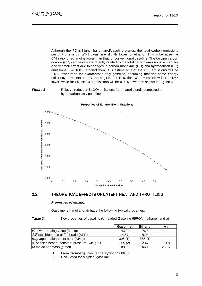
Although the FC is higher for ethanol/gasoline blends, the total carbon emissions per unit of energy (g/MJ basis) are slightly lower for ethanol. This is because the C/H ratio for ethanol is lower than that for conventional gasoline. The tailpipe carbon dioxide (CO2) emissions are directly related to the total carbon emissions, except for a very small effect due to changes in carbon monoxide (CO) and hydrocarbon (HC) emissions. For 100% ethanol then, it is estimated that the CO2 emissions will be 2.6% lower than for hydrocarbon-only gasoline, assuming that the same energy efficiency is maintained by the engine. For E10, the CO2 emissions will be 0.18% lower, while for E5, the CO2 emissions will be 0.09% lower, as shown in Figure 3.

Figure 3 Relative reduction in CO2 emissions for ethanol blends compared to hydrocarbon-only gasoline

Properties of Ethanol Blend Fractions

-3.0%

-2.5%

-2.0%

-1.5%

-1.0%

-0.5%

0.0%

0 0.1 0.2 0.3 0.4 0.5 0.6 0.7 0.8 0.9 1

Ethanol Volume Fraction

CO

2 E

mis

sio

ns

Red

uc

tio

n r

elat

ive

to

Gas

oli

ne

2.3. THEORETICAL EFFECTS OF LATENT HEAT AND THROTTLING

Properties of ethanol

Gasoline, ethanol and air have the following typical properties:

Table 2 Key properties of gasoline (Unleaded Gasoline 95RON), ethanol, and air

Gasoline Ethanol Air Hc lower heating value (MJ/kg) 43.2 26.8 A/F stoichiometric air/fuel ratio (AFR) 14.57 8.94 hvap vaporization latent heat (kJ/kg) 306 (1) 855 (1) cp specific heat at constant pressure (kJ/kg-K) 2.05 (2) 2.47 1.004 M molecular mass (g/mol) 88.6 46.1 28.97

(1) From Bromberg, Cohn and Heywood 2006 [6] (2) Calculated for a typical gasoline

report no. 13/13

6

2.3.1. The effect of airflow and throttling

In stoichiometric Port Fuel Injected (PFI) and Direct Injection (DI) gasoline engines, engine power is controlled by the amount of fuel/air mixture that is allowed into the engine. By altering the position of the throttle valve, more or less air is allowed into the engine and the appropriate amount of fuel is injected downstream, either in the intake port or the cylinder. Since the throttle acts as a restriction to air flow, some energy is lost as the air passes through the throttle, and this loss is greatest when the throttle is at smaller opening positions, i.e. at lower engine loads.

Any change that increases the amount of intake gas needed to produce a given power will require a wider throttle opening to allow the higher volume through; this would directionally improve the efficiency of the engine. Such changes could, of course, affect engine operation in other ways as well, so this is just one factor to consider. As an example, the use of Exhaust Gas Recirculation (EGR) increases the mass of intake gas needed to deliver a given mass of fuel into the engine. For our present purpose, the presence of ethanol in the fuel will affect the air/fuel ratio for stoichiometry and the potential impact of this effect is discussed in this section.

By definition:

cf HmN (1)

Where:

N is power (Watts) η is thermal efficiency

fm is mass flow of fuel (kg/s) and

Hc is the Lower Heating Value of the fuel (J/kg).

Therefore:

cf H

Nm

(2)

For a stoichiometric engine, by definition:

fa mFAm (3)

Where ma is the mass flow of air and A/F is the stoichiometric air-fuel ratio (AFR).

Thus, for a given power N, the following values are obtained:

Gasoline Ethanol

fm fuel mass flow (kg s-1)

gas

kWN

51031.2

EtOH

kWN

51073.3

am air mass flow (kg s-1)

gas

kWN

5107.33

EtOH

kWN

5104.33

With these properties of gasoline and ethanol, there is no significant difference in the air mass flow for both cases, assuming the thermal efficiency is unchanged.

report no. 13/13

7

Thus, with this small change in airflow, throttling should have no significant effect on cycle efficiency.

2.3.2. Effect of latent heat of vaporisation (1)

When using ethanol, the amount of fuel injected and the latent heat of vaporisation are greater. Thus, the final temperature at the end of the intake stroke should be lower. This, in turn, decreases the tendency for engine knock at the end of the compression stroke. Therefore, if the engine is able to adapt its ignition timing, the spark may be advanced for ethanol fuel compared to gasoline. This change may increase the mean effective pressure and, in turn, increase the engine efficiency.

In order to obtain a rough approximation of this effect, the temperature at the end of the intake stroke can be calculated. By definition, the amount of heat needed to evaporate the fuel is given by:

vapf hmQ (4)

Thus, for a given power output, N, the following values are obtained:

Gasoline Ethanol

Q Heat absorbed in vaporization

(kJ/s)

gas

kWN

31008.7

EtOH

kWN

31090.31

This means that, for equal engine efficiencies, the amount of heat needed to evaporate ethanol is 350% greater than that required to evaporate gasoline.

Assuming that the heat is removed from the mixture of fuel and intake air at constant pressure, this heat equals:

TcmTcmQ paapff (5)

Therefore:

paapff cmcm

QT

(6)

Substituting the heat absorbed in the vaporization process:

paapff

vapf

cmcm

hmT

(7)

Finally:

papf

vap

cFAc

hT

(8)

Substituting numbers into this equation gives the following values:

Gasoline Ethanol Temperature difference (ºC) 18.3 74.7

report no. 13/13

8

As was pointed out earlier, this latent heat effect for ethanol reduces the combustion temperature and the tendency of the engine to knock. Therefore, if the engine is able to adapt to the new fuel blend, it can also advance the spark timing in order to take advantage of this cooling effect.

2.3.3. The effect of latent heat (2)

In addition to increasing the efficiency of the engine in some cases (through adaptive spark timing), the extra charge cooling provided by ethanol evaporation, in theory, allows the engine to reach a higher peak power. The following paragraphs offer an explanation of this effect.

On one side, for equal efficiencies, the power of the engine is proportional to the

product cf Hm . On the other side, for a given engine at a given intake

pressure, the maximum amount of air/fuel mixture that can fit inside a cylinder is a consequence of the complete filling of the cylinder, that is, when the engine is charged with the maximum amount of mixture, it is not possible to push more inside.

To a first order approximation, this maximum is given by the final pressure reached at the end of the intake stroke. That is, when the pressure inside the cylinder equals the pressure inside the intake manifold (atmospheric pressure or turbocharger pressure), the air mass flow will stop.

If we assume that the mixture is an ideal gas, then:

RTM

m

M

mRT

M

mnRTpV

f

f

a

a

(9)

Where:

p is pressure V is volume n is the number of moles of gas (air + fuel) R is the universal gas constant T is the temperature m is the mass (ma air or mf fuel) M is molecular mass (Ma air or Mf fuel).

If the engine operates with a stoichiometric mixture, then:

RTMM

FA

mpVfa

f

1 (10)

Thus, the mass of fuel charged inside the cylinder (mf) is:

RT

pV

MMF

Am

fa

f

1

1 (11)

Where:

report no. 13/13

9

p is pressure V is the volume of the cylinder and T is the temperature at the end of the intake stroke.

Up to this point, we have been working with mass flows. However, to apply the ideal gas equation, we also need the mass. This may be done using the following relationship:

e

mm

(12)

Where:

m is the mass charged inside one cylinder m is the mass flow entering the engine ω is the engine speed (in rev/second) and e is the number of admission strokes per revolution of the engine (for a four-

stroke engine, this is the number of cylinders divided by two).

Substituting in the general equation:

RT

epV

MMF

Am

fa

f

1

1 (13)

And multiplying by cH , one obtains:

c

fa

HRT

epV

MMF

AN

1

1

(14)

Where the temperature, T, which appears in the equation represents the temperature at the end of the admission stroke.

If we call θ the temperature of the air in the intake manifold, then the temperature, T, at the end of the admission stroke, allowing for fuel evaporation, is given by:

Gasoline Ethanol T temperature at the end of the admission stroke (in K)

Θ - 18.3 Θ - 74.7

Substituting values into this equation, we obtain:

For gasoline:

3.18

1 01.84 1

KmolkJ

R

epVN

gas (15)

And for ethanol:

report no. 13/13

10

7.74

1 14.81 1

KmolkJ

R

epVN

EtOH (16)

Assuming equal efficiencies for gasoline and ethanol, the power represented by the

factor

R

epV

N

is then given in the following graph (Figure 4):

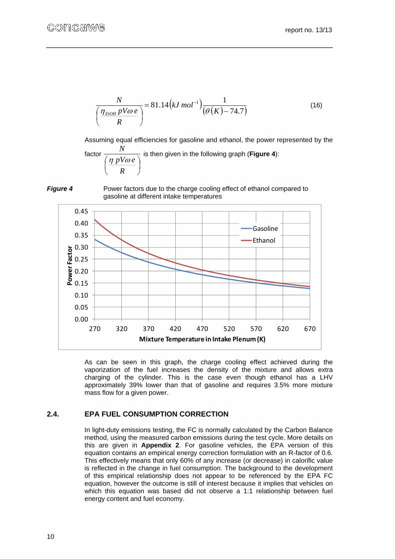
Figure 4 Power factors due to the charge cooling effect of ethanol compared to gasoline at different intake temperatures

0.00

0.05

0.10

0.15

0.20

0.25

0.30

0.35

0.40

0.45

270 320 370 420 470 520 570 620 670

Power Factor

Mixture Temperature in Intake Plenum (K)

Gasoline

Ethanol

As can be seen in this graph, the charge cooling effect achieved during the vaporization of the fuel increases the density of the mixture and allows extra charging of the cylinder. This is the case even though ethanol has a LHV approximately 39% lower than that of gasoline and requires 3.5% more mixture mass flow for a given power.

2.4. EPA FUEL CONSUMPTION CORRECTION

In light-duty emissions testing, the FC is normally calculated by the Carbon Balance method, using the measured carbon emissions during the test cycle. More details on this are given in Appendix 2. For gasoline vehicles, the EPA version of this equation contains an empirical energy correction formulation with an R-factor of 0.6. This effectively means that only 60% of any increase (or decrease) in calorific value is reflected in the change in fuel consumption. The background to the development of this empirical relationship does not appear to be referenced by the EPA FC equation, however the outcome is still of interest because it implies that vehicles on which this equation was based did not observe a 1:1 relationship between fuel energy content and fuel economy.

report no. 13/13

11

3. LITERATURE ASSESSMENT

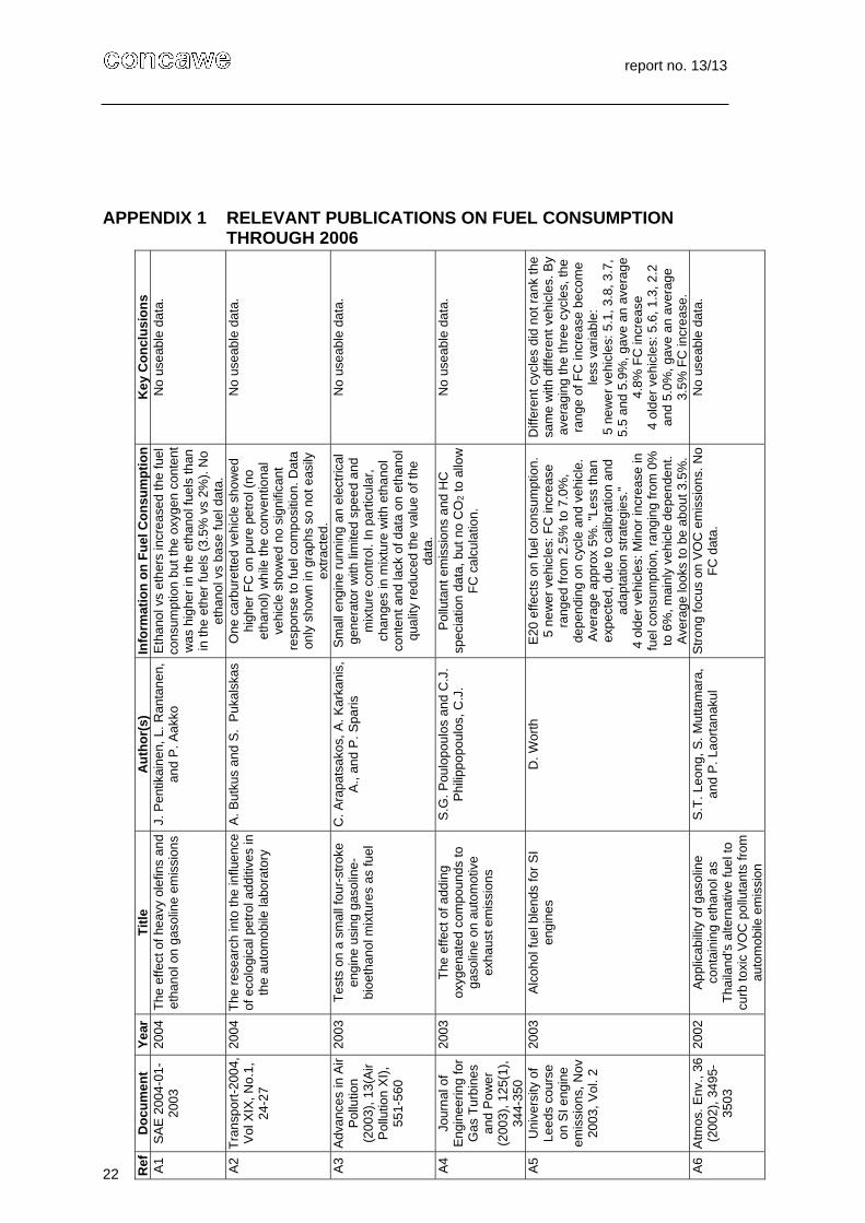
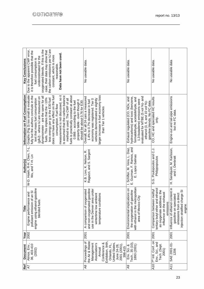
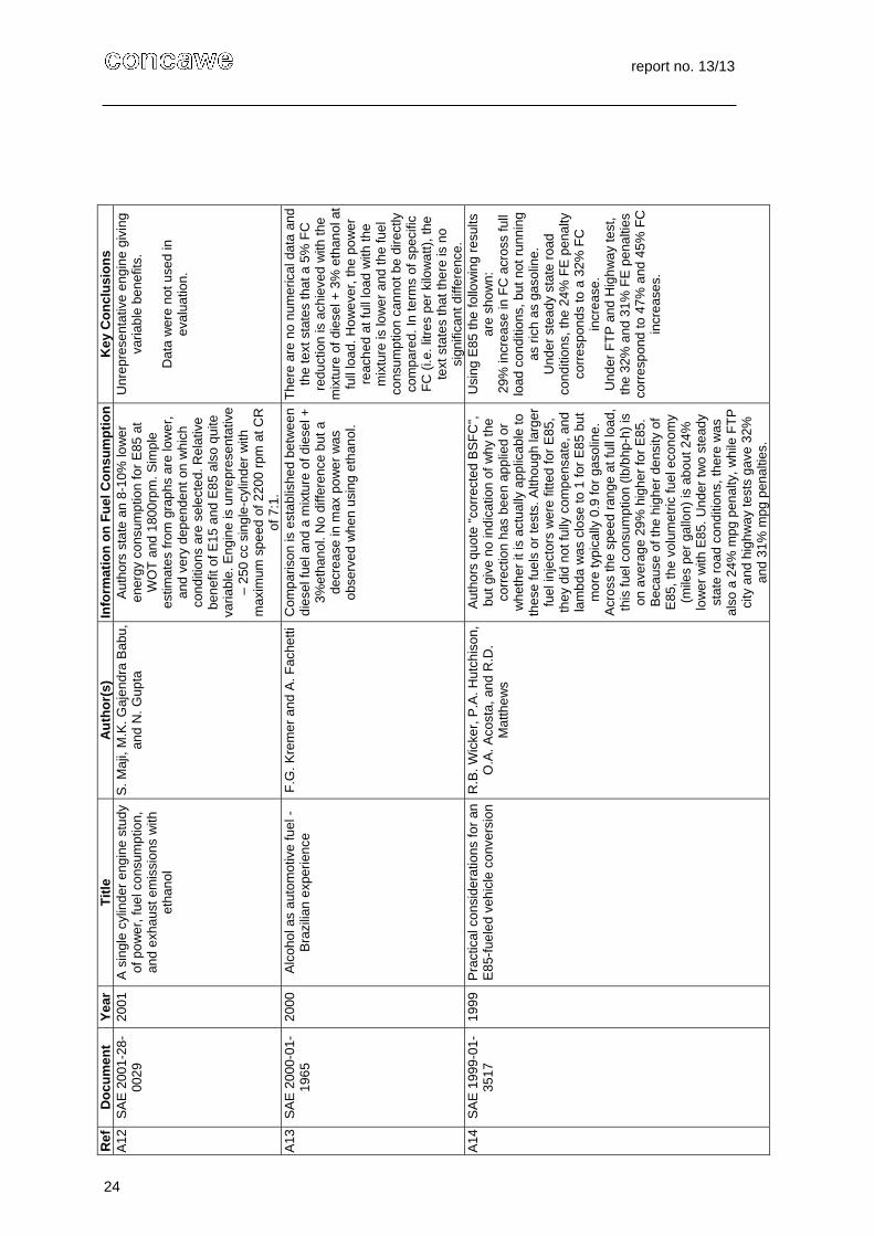
A list of the 29 published studies up to 2006 that were assessed for this report is given in Appendix 1. One of these reports is the JEC study of ethanol effects on evaporative emissions [3] and is covered in more detail in Appendix 3. From the remaining 28 studies, reliable information on the effect of ethanol on fuel consumption was obtained from just 16 studies for the reasons described in Appendix 1.

3.1. INFORMATION ON FUEL CONSUMPTION

Appendix 1 summarises the findings of the studies that provided FC information on low-level ethanol/gasoline blends and shows which data were considered useful for further analysis.

Based on our assessment of these publications, there is not in general a clear picture of the effect of ethanol content on the measured FC. In many cases where more than one vehicle was tested, the results show significant vehicle-to-vehicle variation. For example, reference [A19] (see Appendix 1) shows that the change in volumetric fuel economy (which is the inverse of FC) from the use of E10 varied between a 12.4% increase and a 17.8% decrease. Efficiency changes of this magnitude between vehicles seems unlikely, even if stoichiometry, octane and volatility effects were combined in some manner. Based on the analysis in Section 2 we would expect a 5% decrease in volumetric fuel economy. For this reason, the large variation in results suggests that there were problems with the experimental procedure or measurements.

In other studies, the comparison between different fuels does not appear to be on a fair basis. For example, in reference [A15], the gear ratios of an E85 flexi-fuel vehicle were changed to reduce the engine speed by about 10%. In reference [A21], results obtained on different fuels were compared between a conventional vehicle having a single port injected (SPI) engine and a modified vehicle using multiport injection (MPI) and an improved engine control system running on E95. However, the effect of these high ethanol concentrations in dedicated vehicles is not the main interest of this study.

3.2. FINAL FUEL CONSUMPTION DATA

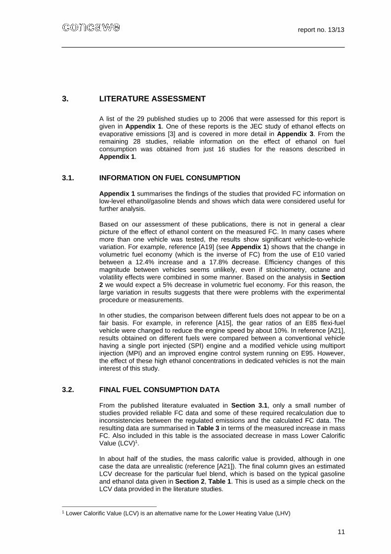
From the published literature evaluated in Section 3.1, only a small number of studies provided reliable FC data and some of these required recalculation due to inconsistencies between the regulated emissions and the calculated FC data. The resulting data are summarised in Table 3 in terms of the measured increase in mass FC. Also included in this table is the associated decrease in mass Lower Calorific Value (LCV)1.

In about half of the studies, the mass calorific value is provided, although in one case the data are unrealistic (reference [A21]). The final column gives an estimated LCV decrease for the particular fuel blend, which is based on the typical gasoline and ethanol data given in Section 2, Table 1. This is used as a simple check on the LCV data provided in the literature studies.

1 Lower Calorific Value (LCV) is an alternative name for the Lower Heating Value (LHV)

report no. 13/13

12

Table 3 Fuel consumption data from published literature studies

Reference

(App 1) Description Fuel Blend

Average reported mass FC increase

Mass LCV decrease

reported in the study

Mass LCV decrease

estimated from Section 2.0

A5 Newer vehicles E20 + 4.8% - 8.05% - 8.0%

A5 Older vehicles E20 + 3.5% - 8.05% - 8.0%

A14 Full load conditions E85 + 29% - 27.2% - 32.6%

A14 Steady state road

conditions E85 + 32% - 27.2% - 32.6%

A14 FTP and highway

tests E85 + 46% - 27.2% - 32.6%

A21 16,000 km of on-road

driving E95 + 37.7%

The reported data gave

- 41.6%, but the gasoline value was incorrect

- 36.2%

A25 NEDC E5 + 0.99% Result not reported

- 2.0%

A26 Hot start (real world)

cycles E10 + 1.24%

Result not reported

- 4.0%

A27 NEDC E5 + 0.18% Result not reported

- 2.0%

A27 NEDC E10 + 2.19% Result not reported

- 4.0%

A28 FTP E10 + 3.7% - 4.4% - 4.0%

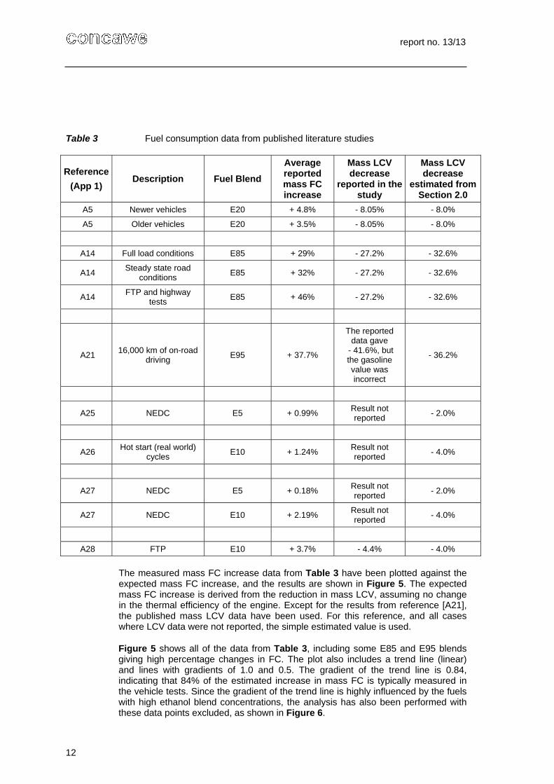
The measured mass FC increase data from Table 3 have been plotted against the expected mass FC increase, and the results are shown in Figure 5. The expected mass FC increase is derived from the reduction in mass LCV, assuming no change in the thermal efficiency of the engine. Except for the results from reference [A21], the published mass LCV data have been used. For this reference, and all cases where LCV data were not reported, the simple estimated value is used.

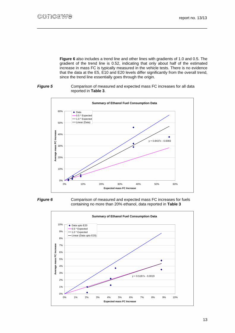
Figure 5 shows all of the data from Table 3, including some E85 and E95 blends giving high percentage changes in FC. The plot also includes a trend line (linear) and lines with gradients of 1.0 and 0.5. The gradient of the trend line is 0.84, indicating that 84% of the estimated increase in mass FC is typically measured in the vehicle tests. Since the gradient of the trend line is highly influenced by the fuels with high ethanol blend concentrations, the analysis has also been performed with these data points excluded, as shown in Figure 6.

report no. 13/13

13

Figure 6 also includes a trend line and other lines with gradients of 1.0 and 0.5. The gradient of the trend line is 0.52, indicating that only about half of the estimated increase in mass FC is typically measured in the vehicle tests. There is no evidence that the data at the E5, E10 and E20 levels differ significantly from the overall trend, since the trend line essentially goes through the origin.

Figure 5 Comparison of measured and expected mass FC increases for all data reported in Table 3.

Summary of Ethanol Fuel Consumption Data

y = 0.8437x - 0.0093

0%

10%

20%

30%

40%

50%

60%

0% 10% 20% 30% 40% 50% 60%

Expected mass FC Increase

Ave

rag

e m

ass

FC

inc

rea

se

Data0.5 * Expected1.0 * ExpectedLinear (Data)

Figure 6 Comparison of measured and expected mass FC increases for fuels containing no more than 20% ethanol, data reported in Table 3

Summary of Ethanol Fuel Consumption Data

y = 0.5187x - 0.0019

0%

1%

2%

3%

4%

5%

6%

7%

8%

9%

10%

0% 1% 2% 3% 4% 5% 6% 7% 8% 9% 10%

Expected mass FC Increase

Ave

rag

e m

ass

FC

incr

eas

e

Data upto E200.5 * Expected1.0 * ExpectedLinear (Data upto E20)

report no. 13/13

14

4. CONCAWE DATA

4.1. JEC EVAPORATIVE EMISSIONS PROGRAMME

While this literature review was in progress, the JEC Consortium also completed an evaporative emissions study on ethanol/gasoline blends [3] and the results from this study were relevant to this report’s FC question.

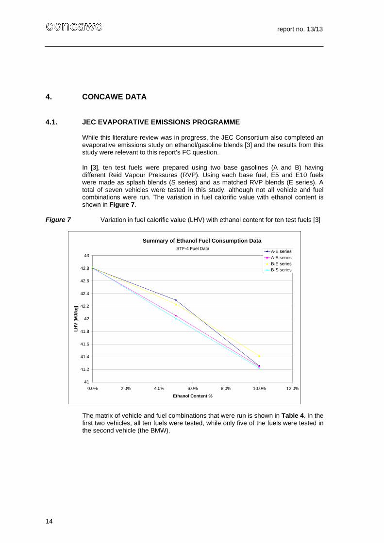
In [3], ten test fuels were prepared using two base gasolines (A and B) having different Reid Vapour Pressures (RVP). Using each base fuel, E5 and E10 fuels were made as splash blends (S series) and as matched RVP blends (E series). A total of seven vehicles were tested in this study, although not all vehicle and fuel combinations were run. The variation in fuel calorific value with ethanol content is shown in Figure 7.

Figure 7 Variation in fuel calorific value (LHV) with ethanol content for ten test fuels [3]

Summary of Ethanol Fuel Consumption Data

41

41.2

41.4

41.6

41.8

42

42.2

42.4

42.6

42.8

43

0.0% 2.0% 4.0% 6.0% 8.0% 10.0% 12.0%

Ethanol Content %

LH

V [

MJ/

kg

]

A-E seriesA-S seriesB-E seriesB-S series

STF-4 Fuel Data

The matrix of vehicle and fuel combinations that were run is shown in Table 4. In the first two vehicles, all ten fuels were tested, while only five of the fuels were tested in the second vehicle (the BMW).

report no. 13/13

15

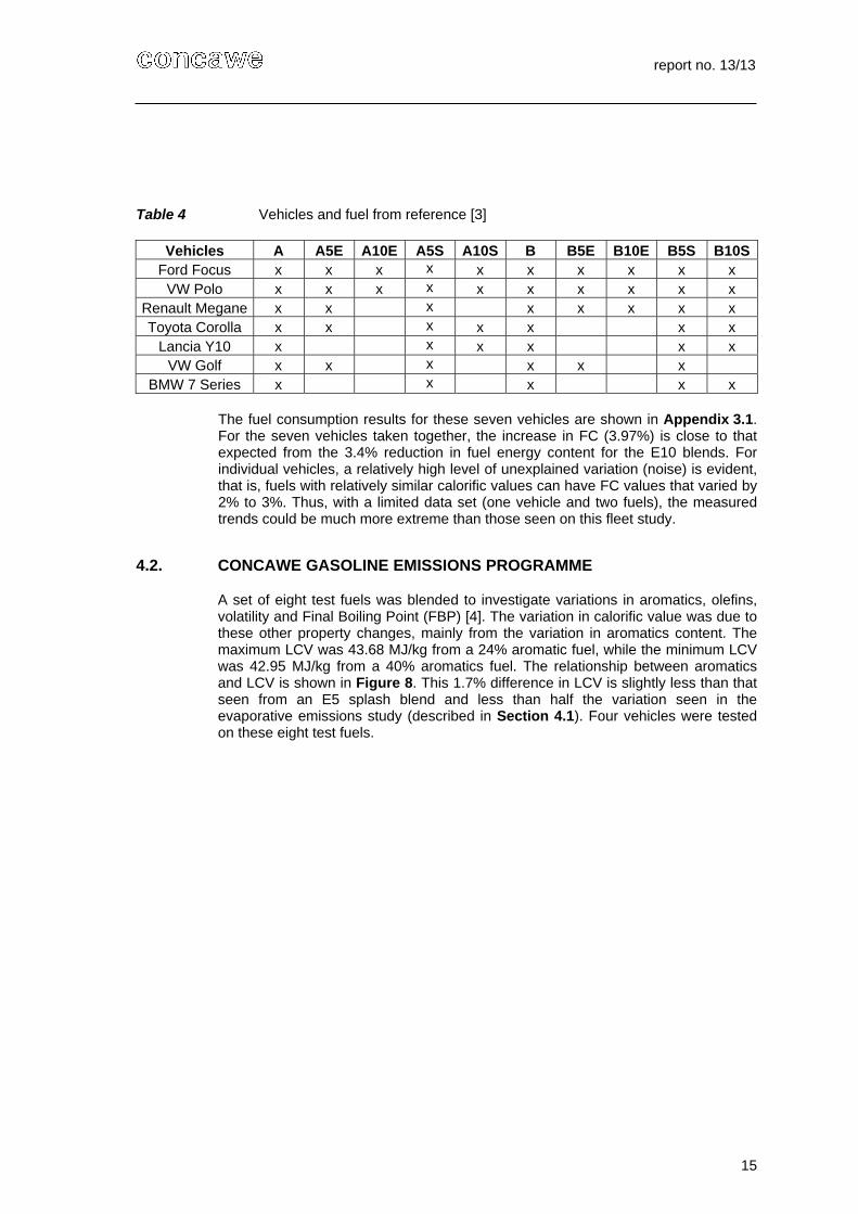
Table 4 Vehicles and fuel from reference [3]

Vehicles A A5E A10E A5S A10S B B5E B10E B5S B10SFord Focus x x x x x x x x x x

VW Polo x x x x x x x x x x Renault Megane x x x x x x x x Toyota Corolla x x x x x x x

Lancia Y10 x x x x x x VW Golf x x x x x x

BMW 7 Series x x x x x

The fuel consumption results for these seven vehicles are shown in Appendix 3.1. For the seven vehicles taken together, the increase in FC (3.97%) is close to that expected from the 3.4% reduction in fuel energy content for the E10 blends. For individual vehicles, a relatively high level of unexplained variation (noise) is evident, that is, fuels with relatively similar calorific values can have FC values that varied by 2% to 3%. Thus, with a limited data set (one vehicle and two fuels), the measured trends could be much more extreme than those seen on this fleet study.

4.2. CONCAWE GASOLINE EMISSIONS PROGRAMME

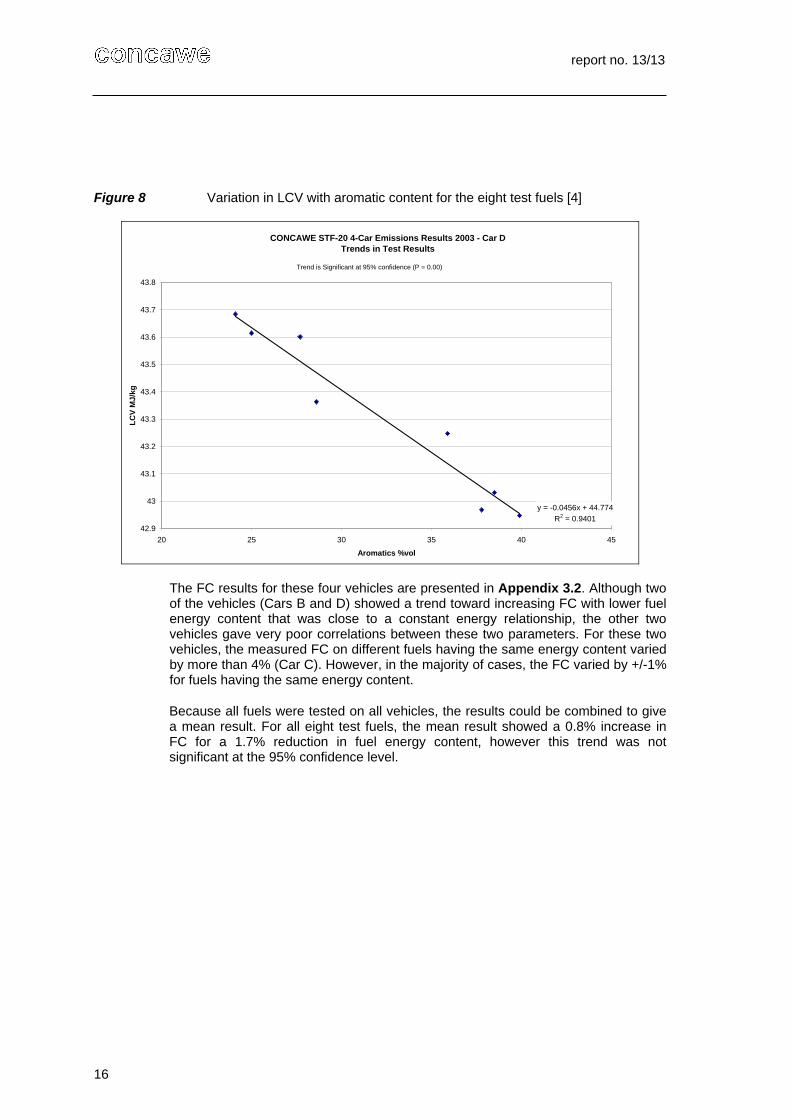
A set of eight test fuels was blended to investigate variations in aromatics, olefins, volatility and Final Boiling Point (FBP) [4]. The variation in calorific value was due to these other property changes, mainly from the variation in aromatics content. The maximum LCV was 43.68 MJ/kg from a 24% aromatic fuel, while the minimum LCV was 42.95 MJ/kg from a 40% aromatics fuel. The relationship between aromatics and LCV is shown in Figure 8. This 1.7% difference in LCV is slightly less than that seen from an E5 splash blend and less than half the variation seen in the evaporative emissions study (described in Section 4.1). Four vehicles were tested on these eight test fuels.

report no. 13/13

16

Figure 8 Variation in LCV with aromatic content for the eight test fuels [4]

CONCAWE STF-20 4-Car Emissions Results 2003 - Car DTrends in Test Results

y = -0.0456x + 44.774

R2 = 0.940142.9

43

43.1

43.2

43.3

43.4

43.5

43.6

43.7

43.8

20 25 30 35 40 45

Aromatics %vol

LC

V M

J/kg

Trend is Significant at 95% confidence (P = 0.00)

The FC results for these four vehicles are presented in Appendix 3.2. Although two of the vehicles (Cars B and D) showed a trend toward increasing FC with lower fuel energy content that was close to a constant energy relationship, the other two vehicles gave very poor correlations between these two parameters. For these two vehicles, the measured FC on different fuels having the same energy content varied by more than 4% (Car C). However, in the majority of cases, the FC varied by +/-1% for fuels having the same energy content.

Because all fuels were tested on all vehicles, the results could be combined to give a mean result. For all eight test fuels, the mean result showed a 0.8% increase in FC for a 1.7% reduction in fuel energy content, however this trend was not significant at the 95% confidence level.

report no. 13/13

17

5. CONCLUSIONS

Theoretically, there are a number of primary and secondary mechanisms through which the blending of ethanol in gasoline can affect the FC of a vehicle over mixed driving conditions.

Lower heating value of ethanol requires a greater mass of fuel to release a given quantity of energy. With an E10 gasoline compared to hydrocarbon-only gasoline, this effect is estimated to increase the FC by 4.2%.

Higher density of ethanol requires a smaller volume of fuel for a given mass. This effect applies only to volumetric FC and is estimated to decrease the volumetric FC by -0.7% for an E10 gasoline compared to hydrocarbon-only gasoline.

The lower carbon weight fraction and higher oxygen content in ethanol reduces the mass of air required to combust a given mass of fuel. This may change the effective mixture strength in the combustion chamber, and thus change the combustion efficiency of the engine.

The combination of heating value and stoichiometry will affect the airflow requirements at a given engine power output. This will impact the throttle setting, which has a strong influence on the overall efficiency of the engine.

The volume of fuel in the cylinder depends on the fuel’s mass and density. For ethanol, the mass will be higher due to the low heating value and the density (as a gas) will be lower due to ethanol’s relatively low molecular weight compared to gasoline. In the combustion chamber, the greater the volume occupied by fuel, the lower the volume available for air, and thus the need to reduce throttling in order to maintain the air flow.

The higher octane value of ethanol may allow the engine to operate under more optimised ignition timing regimes at higher loads (if these are encountered during the test cycle), leading to higher combustion efficiency. The engine could potentially be adapted to take advantage of this effect.

The very high latent heat of vaporisation of ethanol can potentially provide a high level of charge air cooling, increasing the air density and thus the mass of fuel in the cylinder. This may also impact the throttle setting, as mentioned above.

Different volatility characteristics for ethanol and a higher heat of vaporisation could result in changes to fuel-air mixing and combustion characteristics. The magnitude of this effect on FC was not estimated in this report.

Ethanol could also introduce chemical kinetic effects on the laminar flame speed and thus the combustion efficiency. The magnitude of this effect on FC was not estimated in this report.

report no. 13/13

18

Our review of the published literature through 2006 resulted in the following conclusions:

There was a relatively high incidence of incorrectly derived FC data, usually resulting in an underestimate of the FC for ethanol-containing fuels. In some cases this was due to the use of an unadjusted carbon weight fraction in the carbon-balance equation. In other cases, the EPA gasoline equation was used which attempts to correct for differences in fuel calorific value.

For tests with fuel blends up to E20, the typical increase in mass FC was about 50% of the expected value, based simply on the decrease in calorific value with ethanol addition. For example, for an E10 blend, a 2% mass FC increase was measured compared to the 4% expected from the decrease in calorific value when ethanol was added.

From the information provided above, it is estimated that approximately 50% of the increase in mass FC is compensated by the listed mechanisms.

From the analysis of the two CONCAWE vehicle and fuel studies [3,4], the following conclusions can be made:

In the most extreme case, fuels with almost identical energy content showed a FC difference of more than 4%, although for the majority of vehicles the difference was generally less than 2%.

This variation in FC did not appear to be related to fuel parameters other than the ethanol content. However, if it were due to other parameters, the effects are vehicle specific. Based on the results, it is assumed that the variation in results are most likely due to measurement variability (noise).

This level of variability affects the conclusions that can be drawn on the impact of low levels of ethanol in gasoline on FC unless the experimental study is specially designed to answer the FC question. Consumers are unlikely to see small FC effects in real world driving but the quantitative impact of ethanol on FC is important on a fuel demand and CO2 emissions perspective.

For the largest data set (7 vehicles using up to 10 test fuels), the overall trend showed a 3.97% increase in FC with a 3.4% reduction in fuel energy content. However, the evaluation of individual vehicles with more limited fuel sets could lead to very different conclusions.

These conclusions suggested that a more definitive vehicle study was warranted to determine whether modern vehicles can compensate for the lower energy content of ethanol-containing gasolines through better engine efficiency. Such a study has been completed by the JEC Consortium and will be reported separately [5].

report no. 13/13

19

6. GLOSSARY

A/F Air / Fuel

AFR Air / Fuel Ratio

CO Carbon Monoxide

CO2 Carbon Dioxide

CR Compression Ratio

CWF Carbon Weight Fraction

DVPE Dry Vapour Pressure Equivalent

E5 / E10 / E20 2.7 / 3.7 / 7.4 wt% oxygen in gasoline, which is equivalent to 5 / 10 / 20% v/v ethanol in gasoline

E85 85% v/v ethanol in gasoline

EGR Exhaust Gas Recirculation

EN 228 European standard for automotive gasoline

EPA Environmental Protection Agency (USA)

EUCAR European Council for Automotive R&D

FBP Final Boiling Point

FC Fuel consumption

FFV Flexi-Fuel Vehicle

FTP Federal Test Procedure

HC Hydrocarbon

JEC JRC/EUCAR/CONCAWE

JRC Joint Research Centre (of the European Commission)

LCV Lower Calorific Value (same as LHV)

LHV Lower Heating Value (same as LCV)

MJ Megajoule

MPGE Miles Per Gallon Equivalent

MPI Multi Port Injection

NEDC New European Driving Cycle

RON Research Octane Number

rpm revolutions per minute

RVP Reid Vapour Pressure

SPI Single Port Injection

WOT Wide Open Throttle

WTW Well-to-Wheels

report no. 13/13

20

7. ACKNOWLEDGMENTS

This literature assessment was initiated by Neville Thompson who was CONCAWE’s Technical Coordinator for Fuels and Emissions before his untimely death in 2006. Through his co-authorship of this report, it is our privilege to recognise once again his important contributions to CONCAWE’s work in the area of fuels and vehicle emissions.

report no. 13/13

21

8. REFERENCES

1. JEC (2011) Well-to-wheels analysis of future automotive fuels and powertrains in the European context. Well-to-wheels report, version 3c. Report EUR 24952 EN-2011. Brussels: JRC, EUCAR, CONCAWE

2. EU (2009) Ethanol/petrol blends: volatility characterisation in the range 5-25 vol% ethanol (BEP525). TREN/D2/454-2008-SI.2.522.698, Final report. Brussels: EU Commission

3. JEC (2007) Effects of gasoline vapour pressure and ethanol content on evaporative emissions from modern cars. Report EUR 22713 EN. Brussels: JRC, EUCAR, CONCAWE

4. CONCAWE (2004) Fuel effects on emissions from modern gasoline vehicles. Part 2 – aromatics, olefins, and volatility effects. Report No. 2/04. Brussels: CONCAWE

5. JEC (2013) Effect of oxygenates in gasoline on fuel consumption and emissions in three Euro 4 passenger cars. Report EUR 26381 EN. Brussels: JRC, EUCAR, CONCAWE

6. Bromberg, L. et al (2006) Calculations of knock suppression in highly turbocharged gasoline/ethanol engines using direct ethanol injection. Cambridge MA: Massachusetts Institute of Technology

report no. 13/13

22

APPENDIX 1 RELEVANT PUBLICATIONS ON FUEL CONSUMPTION THROUGH 2006

Ref

D

ocu

men

tY

ear

Tit

le

Au

tho

r(s)

Info

rmat

ion

on

Fu

el C

on

sum

pti

on

Key

Co

ncl

usi

on

sA

1 S

AE

200

4-01

-20

03

20

04

The

effe

ct o

f hea

vy o

lefin

s a

nd

etha

nol

on

gaso

line

emis

sion

sJ.

Pen

tikai

nen

, L.

Ran

tan

en,

and

P. A

akko

E

than

ol v

s et

her

s in

cre

ased

the

fuel

co

nsum

ptio

n b

ut t

he o

xyg

en

cont

ent

wa

s hi

gher

in th

e et

hano

l fue

ls th

an

in th

e et

her

fue

ls (

3.5%

vs

2%).

No

etha

nol

vs

base

fuel

dat

a.

No

use

able

dat

a.

A2

Tra

nspo

rt-2

004,

V

ol X

IX,

No.

1,

24-2

7

200

4T

he r

esea

rch

into

the

influ

ence

of

eco

logi

cal p

etro

l ad

ditiv

es in

th

e au

tom

obi

le la

bora

tory

A. B

utku

s an

d S

. P

ukal

skas

One

car

bure

tted

vehi

cle

sho

wed

hi

ghe

r F

C o

n p

ure

petr

ol (

no

etha

nol

) w

hile

the

conv

entio

nal

vehi

cle

sho

we

d no

sig

nific

ant

resp

onse

to

fuel

com

pos

itio

n. D

ata

only

sh

ow

n in

gra

phs

so

not

easi

ly

extr

acte

d.

No

use

able

dat

a.

A3

Adv

ance

s in

Air

P

ollu

tion

(200

3), 1

3(A

ir P

ollu

tion

XI)

, 55

1-56

0

200

3T

ests

on

a sm

all f

our-

stro

ke

eng

ine

usin

g g

asol

ine-

bio

etha

nol m

ixtu

res

as fu

el

C.

Ara

pats

ako

s, A

. Kar

kani

s,

A.,

and

P. S

paris

S

mal

l eng

ine

runn

ing

an e

lect

rical

ge

ner

ator

with

lim

ited

spee

d a

nd

mix

ture

con

tro

l. In

par

ticul

ar,

chan

ges

in m

ixtu

re w

ith e

tha

nol

co

nten

t and

lack

of d

ata

on e

than

ol

qua

lity

redu

ced

the

valu

e of

the

data

.

No

use

able

dat

a.

A4

Jour

nal

of

Eng

inee

rin

g fo

r G

as T

urbi

nes

and

Po

we

r (2

003)

, 125

(1),

34

4-35

0

200

3T

he e

ffect

of a

ddin

g ox

yge

nate

d co

mpo

und

s to

ga

solin

e on

aut

omot

ive

exha

ust e

mis

sion

s

S.G

. Pou

lopo

ulos

and

C.J

. P

hilip

pop

oulo

s, C

.J.

Pol

luta

nt e

mis

sion

s a

nd H

C

spec

iatio

n da

ta,

but n

o C

O2 t

o al

low

F

C c

alcu

latio

n.

No

use

able

dat

a.

A5

Uni

vers

ity o

f Le

eds

cou

rse

on S

I eng

ine

emis

sion

s, N

ov

200

3, V

ol. 2

200

3A

lcoh

ol fu

el b

lend

s fo

r S

I en

gin

es

D. W

orth

E

20 e

ffect

s on

fue

l con

sum

ptio

n.

5 ne

we

r ve

hicl

es: F

C in

crea

se

rang

ed fr

om 2

.5%

to 7

.0%

, de

pen

din

g on

cyc

le a

nd

vehi

cle.

A

vera

ge

appr

ox

5%. "

Les

s th

an

expe

cte

d, d

ue t

o ca

libra

tion

and

ad

apt

atio

n st

rate

gies

."

4 ol

der

veh

icle

s: M

inor

incr

ea

se in

fu

el c

onsu

mpt

ion,

ran

gin

g fr

om 0

%

to 6

%, m

ainl

y ve

hicl

e de

pend

ent

. A

vera

ge

look

s to

be

abou

t 3.5

%.

Diff

eren

t cyc

les

did

not r

ank

the

sam

e w

ith d

iffer

ent v

ehic

les.

By

aver

agi

ng

the

thre

e cy

cles

, the

ra

nge

of F

C in

crea

se b

ecom

e le

ss v

aria

ble:

5

new

er

vehi

cles

: 5.1

, 3.8

, 3.7

, 5.

5 an

d 5.

9%, g

ave

an

aver

age

4.

8% F

C in

crea

se

4 ol

der

veh

icle

s: 5

.6, 1

.3, 2

.2

and

5.0

%, g

ave

an a

vera

ge

3.5%

FC

incr

eas

e.

A6

Atm

os.

Env

., 36

(2

002)

, 349

5-35

03

200

2A

pplic

abili

ty o

f gas

olin

e co

ntai

nin

g et

hano

l as

Tha

iland

's a

ltern

ativ

e fu

el t

o cu

rb to

xic

VO

C p

ollu

tant

s fr

om

auto

mo

bile

em

issi

on

S.T

. Le

ong,

S. M

utta

mar

a,

and

P. L

aor

tan

akul

S

tron

g fo

cus

on

VO

C e

mis

sio

ns. N

o F

C d

ata.

N

o us

eab

le d

ata.

report no. 13/13

23

Ref

D

ocu

men

tY

ear

Tit

le

Au

tho

r(s)

Info

rmat

ion

on

Fu

el C

on

sum

pti

on

Key

Co

ncl

usi

on

sA

7 A

tmos

. E

nv.,

36, 4

03-4

10

(200

2)

200

2E

ngin

e p

erfo

rman

ce a

nd

pollu

tant

em

issi

on o

f an

SI

eng

ine

usin

g et

han

ol-g

aso

line

ble

nde

d fu

els

W-D

. Hsi

eh, R

-H. C

hen,

T-L

. W

u, a

nd T

-H. L

in

Gra

phs

(Fig

3)

too

smal

l to

eval

uat

e fu

lly b

ut th

e a

utho

rs c

oncl

ude

in th

e te

xt th

at m

ass

fuel

co

nsum

ptio

n (g

/kJ)

- w

here

kJ

are

mea

sure

d on

d

ynam

omet

er -

are

the

sam

e fo

r al

l fu

els.

Thi

s im

plie

s th

at th

e ~

10%

le

ss e

ner

gy

pe

r g

in th

e E

30 f

uel

does

not

hav

e an

y ef

fect

on

the

fuel

co

nsum

ptio

n. F

uel f

low

m

easu

rem

ent i

s no

t dis

cuss

ed,

so

it is

ass

ume

d th

at

the

carb

on b

ala

nce

met

hod

is u

sed

. The

CW

F o

f all

fuel

s is

pra

ctic

ally

co

nsta

nt a

t ab

out

0.86

6 –

acco

rdin

g to

the

fue

l pr

oper

ty ta

ble

- e

ven

tho

ugh

it sh

ould

be

abo

ut 0

.76

for

E30

.

Due

to th

e a

ppar

ent C

WF

err

or,

it is

ther

efor

e p

ossi

ble

that

the

fu

el c

onsu

mpt

ion

is

und

eres

timat

ed

for

the

oxyg

enat

ed b

lend

s. I

f th

is is

the

ca

se, t

heir

data

ma

y sh

ow

that

th

e ca

rbo

n em

issi

ons

per

kJ

are

cons

tant

, w

hich

is m

ore

reas

ona

ble

. D

ata

ha

ve n

ot

bee

n u

sed

.

A8

Pro

cee

din

gs o

f th

e A

ir &

Was

te

Man

age

me

nt

Ass

ocia

tion'

s A

nnu

al

Con

fere

nce

&

Exh

ibiti

on,

94th

, O

rland

o, F

L,

Uni

ted

Sta

tes,

Ju

ne 2

4-2

8,

200

1 (2

001

),

398-

415

200

1A

com

paris

on o

f oxy

gen

ated

an

d n

on-o

xyge

nate

d g

aso

line

use

in th

e D

enve

r ar

ea u

nder

w

inte

rtim

e lo

w a

mbi

ent

tem

pera

ture

co

nditi

ons

K.B

. Li

vo,

K.

Nel

son,

R.

Rag

azzi

, an

d S

. Sar

gent

O

vera

ll, fo

r al

l 24

cars

a m

easu

red

1.4%

to 0

.7%

dec

reas

e in

fue

l ec

onom

y w

as

regi

ster

ed. T

ier

0 ve

hicl

es d

emo

nstr

ated

a s

ligh

tly

larg

er in

cre

ase

in fu

el e

cono

my

loss

th

an T

ier

1 ve

hic

les

No

use

able

dat

a.

A9

Env

. S

ci.

&

Tec

h., 3

5 (1

0),

189

3 (2

001

)

200

1E

nviro

nmen

tal i

mpl

icat

ions

on

th

e o

xyge

natio

n of

gas

olin

e w

ith e

tha

nol i

n th

e m

etro

polit

an

area

of M

exi

co C

ity

I. S

chift

er,

M. V

era,

L.

Dia

z,

E. G

uzm

an, F

. Ram

os, a

nd

E. L

opez

-Sa

linas

Exh

aust

reg

ula

ted

(CO

, NO

x, a

nd

hyd

roca

rbo

ns)

and

toxi

c (b

enze

ne,

form

ald

ehyd

e, a

ceta

lde

hyd

e, a

nd

1,3-

buta

dien

e) e

mis

sio

ns w

ere

eval

uate

d fo

r M

TB

E (

5 vo

l %)-

and

et

han

ol (

3, 6

, and

10

vol %

)-ga

solin

e bl

end

s. N

o F

C d

ata.

No

use

able

dat

a.

A10

7th

Intl.

Con

f. on

E

nv.,

Sci

., an

d T

ech.

(S

ept.

200

1)

200

1C

omp

aris

on

betw

een

met

hyl

te

rtia

ry b

utyl

eth

er a

nd

etha

nol

as o

xyge

nate

add

itive

s: th

e in

fluen

ce o

n th

e e

xha

ust

emis

sion

s

S.G

. Pou

lopo

ulos

and

C.J

. P

hilip

pop

oulo

s C

O, H

C a

nd s

pec

iate

d H

C r

esul

ts

only

. N

o us

eab

le d

ata.

A11

S

AE

200

1-01

-12

06

20

01

Influ

ence

of e

than

ol c

ont

ent i

n ga

solin

e on

sp

ecia

ted

emis

sio

ns fr

om a

dire

ct

inje

ctio

n st

ratif

ied

char

ge S

I en

gin

e

H. S

andq

uist

, M. K

arls

son,

an

d I.

Den

brat

t E

ngin

e-o

ut a

nd ta

il-pi

pe e

mis

sion

s bu

t no

FC

dat

a.

No

use

able

dat

a

report no. 13/13

24

Ref

D

ocu

men

tY

ear

Tit

le

Au

tho

r(s)

Info

rmat

ion

on

Fu

el C

on

sum

pti

on

Key

Co

ncl

usi

on

sA

12

SA

E 2

001-

28-

002

9

200

1A

sin

gle

cylin

der

eng

ine

stu

dy

of p

ow

er, f

uel c

onsu

mpt

ion,

an

d e

xha

ust e

mis

sion

s w

ith

etha

nol

S. M

aji,

M.K

. Gaj

end

ra B

abu,

an

d N

. Gup

ta

Aut

hors

sta

te a

n 8-

10%

low

er

ener

gy

cons

um

ptio

n fo

r E

85 a

t W

OT

and

180

0rp

m. S

impl

e es

timat

es fr

om g

raph

s ar

e lo

we

r,

and

very

dep

end

ent

on

wh

ich

co

nditi

ons

are

sele

cte

d. R

elat

ive

ben

efit

of E

15 a

nd E

85

also

qui

te

varia

ble.

En

gin

e is

unr

epr

ese

ntat

ive

– 25

0 cc

sin

gle

-cyl

ind

er w

ith

max

imum

sp

eed

of 2

200

rpm

at C

R

of 7

:1.

Unr

epr

ese

ntat

ive

eng

ine

givi

ng

varia

ble

bene

fits.

Dat

a w

ere

not u

sed

in

eval

uatio

n.

A13

S

AE

200

0-01

-19

65

20

00A

lcoh

ol a

s au

tom

otiv

e fu

el -

B

razi

lian

exp

erie

nce

F

.G. K

rem

er a

nd A

. Fac

hetti

Com

par

iso

n is

est

ablis

hed

betw

ee

n di

esel

fuel

and

a m

ixtu

re o

f die

sel +

3%

eth

anol

. No

diff

eren

ce b

ut a

de

cre

ase

in m

ax p

ow

er

was

ob

serv

ed w

hen

usi

ng e

than

ol.

The

re a

re n

o n

umer

ica

l dat

a an

d th

e te

xt s

tate

s th

at a

5%

FC

re

duct

ion

is a

chie

ved

with

the

m

ixtu

re o

f die

sel +

3%

eth

ano

l at

full

load

. Ho

we

ver,

the

pow

er

reac

hed

at f

ull l

oad

with

the

mix

ture

is lo

we

r an

d th

e fu

el

cons

umpt

ion

cann

ot b

e di

rect

ly

com

pare

d. In

term

s of

spe

cific

F

C (

i.e. l

itres

per

kilo

wa

tt), t

he

text

sta

tes

that

ther

e is

no

sign

ifica

nt d

iffe

renc

e.

A14

S

AE

199

9-01

-35

17

19

99

Pra

ctic

al c

ons

ider

atio

ns fo

r a

n E

85-f

uele

d ve

hic

le c

onv

ersi

onR

.B. W

icke

r, P

.A. H

utch

ison

, O

.A.

Aco

sta,

and

R.D

. M

atth

ew

s

Aut

hors

qu

ote

"cor

rect

ed B

SF

C",

bu

t giv

e n

o in

dica

tion

of w

hy

the

corr

ectio

n ha

s be

en

appl

ied

or

wh

eth

er it

is a

ctua

lly a

pplic

abl

e to

th

ese

fuel

s or

test

s. A

lthou

gh

larg

er

fuel

inje

ctor

s w

ere

fitte

d fo

r E

85,

the

y di

d n

ot fu

lly c

omp

ensa

te, a

nd

lam

bda

was

clo

se to

1 fo

r E

85

but

mor

e ty

pic

ally

0.9

for

gaso

line.

A

cros

s th

e sp

eed

ran

ge a

t ful

l loa

d,

this

fuel

con

sum

ptio

n (l

b/bh

p-h)

is

on a

vera

ge

29%

hig

her

for

E85

. B

ecau

se o

f the

hig

her

de

nsity

of

E85

, the

vol

umet

ric fu

el e

cono

my

(mile

s pe

r ga

llon)

is a

bout

24

%

low

er w

ith E

85.

Und

er t

wo

ste

ady

stat

e ro

ad c

on

ditio

ns, t

here

was

al

so a

24%

mp

g pe

nal

ty,

wh

ile F

TP

ci

ty a

nd h

igh

wa

y te

sts

gave

32%

an

d 3

1% m

pg

pen

altie

s.

Usi

ng E

85 th

e fo

llow

ing

resu

lts

are

sho

wn

: 29

% in

crea

se in

FC

acr

oss

full

loa

d co

ndi

tions

, but

not

run

nin

g as

ric

h as

gas

olin

e.

Und

er s

tead

y st

ate

road

co

nditi

ons,

the

24%

FE

pen

alty

co

rres

pon

ds to

a 3

2% F

C

incr

ease

. U

nder

FT

P a

nd H

igh

wa

y te

st,

the

32%

and

31%

FE

pen

alti

es

corr

esp

ond

to 4

7% a

nd 4

5% F

C

incr

ease

s.

report no. 13/13

25

Ref

D

ocu

men

tY

ear

Tit

le

Au

tho

r(s)

Info

rmat

ion

on

Fu

el C

on

sum

pti

on

Key

Co

ncl

usi

on

sA

15

SA

E 1

999-

01-

356

8

199

9Im

prov

ing

the

fuel

effi

cien

cy o

f lig

ht-d

uty

etha

nol v

ehi

cles

--A

n en

gin

e d

ynam

omet

er s

tud

y o

f de

dic

ate

d en

gin

e st

rate

gies

D.P

. G

ardi

ner,

R.W

. M

allo

ry,

Rob

ert

W.

(Nex

um R

esea

rch

Cor

por

atio

n); P

uche

r, G

reg

R. (

Nex

um R

ese

arch

C

orp

orat

ion)

; Tod

esco

, Mar

c K

. (N

exum

Res

earc

h C

orp

orat

ion)

; Bar

don,

M

icha

el F

. (R

oya

l Mili

tary

C

olle

ge

of C

anad

a); M

arke

l, T

ony

J

If th

e dr

ivel

ine

gear

ing

of a

de

dic

ate

d E

85 v

ehic

le w

as c

han

ged

to

red

uce

the

eng

ine

spee

d b

y ab

out

10%

it

wo

uld

be p

ossi

ble

for

a de

dic

ate

d E

85

eng

ine

to a

chie

ve

fuel

eco

nom

y im

prov

emen

ts o

f ab

out

15%

(M

PG

E b

asis

) ov

er a

co

mpa

rabl

e ga

solin

e en

gine

. R

educ

ing

the

spee

d of

the

ded

icat

ed

E85

eng

ine

will

pro

vide

gr

eate

r re

lativ

e im

prov

emen

ts in

fuel

ec

onom

y un

der

oper

atin

g co

ndi

tions

ty

pica

lly o

ccur

ring

dur

ing

urb

an

driv

ing

(i.e.

, lo

we

r av

erag

e p

ow

er)

than

thos

e w

hich

occ

ur d

urin

g hi

gh

wa

y dr

ivin

g.

No

use

able

dat

a

A16

K

FB

-M

edd

ela

nde

Pub

licat

ion

199

9:4

199

9M

oder

ate

addi

tions

of a

lcoh

ols

to g

asol

ine.

La

agin

blan

dnin

g av

alk

oho

ler

i ben

sin.

A. L

aves

kog

and

K-E

. E

geb

aeck

O

ld v

ehic

les

and

not

rel

eva

nt te

st

cycl

e.

No

use

able

dat

a

A17

S

AE

199

9-01

-35

70

19

99

Effe

ct o

f gas

olin

e co

mp

ositi

on

s an

d pr

oper

ties

on ta

ilpip

e em

issi

ons

of c

urre

ntly

exi

stin

g ve

hicl

es in

Tha

ilan

d

T. T

hum

mad

etsa

k, A

. W

uttim

ongk

olc

hai,

S.

Tun

yap

iset

sak,

and

T.

Kim

ura

TH

C, C

O, N

Ox

and

air

toxi

c em

issi

ons

, but

no

FC

dat

a.

No

use

able

dat

a

A18

S

AE

982

531

19

98

Fin

al r

esul

ts fr

om th

e S

tate

of

Ohi

o et

hano

l-fue

lled,

ligh

t-d

uty

fleet

dep

loym

ent

pro

ject

K. C

hand

ler,

M. W

hale

n, a

nd

J. W

esth

oven

O

ld F

FV

veh

icle

usi

ng

E85

(+

33%

F

C r

epor

ted)

N

o us

eab

le d

ata

A19

J.

Air

& W

aste

M

gmt.

Ass

oc.,

48, 6

46 (

199

8)

199

8T

he e

ffect

of e

than

ol fu

el o

n th

e em

issi

ons

of v

ehic

les

ove

r a

wid

e ra

nge

of

tem

pera

ture

s

K.T

. K

napp

, F.D

. Stu

mp,

and

S

.B. T

ejad

a F

uel E

con

omy:

Hig

hly

varia

ble

(veh

icle

to v

ehic

le).

Vol

umet

ric

fuel

ec

onom

y (m

iles/

gal)

ran

ged

from

12

.4%

incr

ease

(be

tter)

to 1

7.8%

de

cre

ase

(wor

se).

Ave

rage

val

ue

wa

s cl

ose

to z

ero.

Dat

a to

o v

ari

able

to

be

use

d

relia

bly

.

report no. 13/13

26

Ref

D

ocu

men

tY

ear

Tit

le

Au

tho

r(s)

Info

rmat

ion

on

Fu

el C

on

sum

pti

on

Key

Co

ncl

usi

on

sA

20

SA

E 9

608

55

199

6C

ompr

ehe

nsiv

e la

bor

ator

y fu

el

econ

omy

test

ing

with

RF

G a

nd

conv

ent

iona

l fu

els

T.A

. K

elln

er,

K.

Neu

sen,

D.

Bre

sen

ham

, M. P

ike,

and

D.

Ros

e

The

ave

rage

flee

t fue

l eco

nom

y re

duct

ion

gen

era

lly m

irror

ed th

e ex

pect

ed

fuel

eco

nom

y re

duct

ion.

T

he tr

ansi

ent b

ased

IM24

0 te

sts

did

not e

xhib

it th

e ex

pect

ed

fuel

ec

onom

y re

duct

ions

bas

ed o

n en

erg

y co

nte

nt r

educ

tion.

The

di

strib

utio

n of

the

test

ed v

ehi

cle/

fuel

m

atrix

sh

ow

ed

that

a p

ortio

n o

f th

e te

st v

ehic

les

expe

rienc

ed e

xces

sive

fu

el e

cono

my

redu

ctio

n a

nd

incr

eas

es. N

o on

e co

ntro

l sys

tem

ex

hibi

ted

the

gre

ates

t fue

l eco

nom

y de

viat

ion

(re

duct

ion

and

incr

eas

es).

N

o R

FG

con

sist

ently

cau

sed

exce

ssiv

e fu

el e

con

omy

redu

ctio

n or

ga

ins.

No

use

able

dat

a

A21

S

AE

952

749

19

95

A c

ompa

rativ

e an

aly

sis

of

etha

nol

ver

sus

gaso

line

as a

fu

el in

pro

duc

tion

four

-str

oke

cycl

e au

tom

otiv

e en

gin

es

B. J

ones

, K. R

ead

y, R

. Bac

h,

D. H

anse

n, E

. Kai

tala

, J.

Lars

on,

J. M

oral

es, a

nd

C.

Ree

se

Eng

ine

har

dw

are

cha

nge

s in

clud

ed

CR

incr

eas

e a

nd ig

nitio

n tim

ing

optim

isat

ion.

20.

0 km

/litr

e on

ga

solin

e an

d 1

4.52

km

/litr

e o

n E

95.

The

ir LC

V v

alu

es (

in M

J/kg

) a

re

inco

rrec

t, an

d in

Btu

/lb a

re

reas

ona

ble

for

E95

, but

for

gaso

line

it is

too

high

. Usi

ng th

eir

fuel

LC

V

data

, the

y ca

lcul

ate

bet

ter

ener

gy

effic

ienc

y fo

r th

e E

95 v

ehic

le,

how

eve

r by

rec

alcu

latin

g (f

rom

es

timat

ed L

CV

and

de

nsiti

es)

som

e of

this

ben

efit

disa

ppe

ars.

FC

is 3

7.7%

gre

ater

from

E95

fu

el. F

rom

a r

ecal

cula

ted

ener

gy

basi

s, w

e w

oul

d e

xpec

t it t

o b

e 45

.4%

hig

her.

A22

E

MP

A R

epor

t 20

2,6

72 (

Se

pt.

200

2)

200

2B

io-e

than

ol P

roje

kt -

Pot

entia

l de

r bi

o-et

han

ol b

eim

isch

ung

im b

enzi

n un

d di

esel

-tre

ibst

off

unte

rsuc

hung

en

hins

icht

lich

des

emis

sion

sver

halte

ns a

n ei

nem

nut

zfah

rzeu

g m

otor

un

d zw

ei p

erso

nen

fahr

zeug

en

U. L

ehm

ann

T

abul

ated

dat

a d

oes

not i

nclu

de

CO

2 o

r F

C.

No

use

able

dat

a

A23

C

AR

B R

epo

rt

(Dec

. 199

9)

199

9A

ir qu

alit

y im

pac

ts o

f the

use

of

eth

anol

in C

alifo

rnia

re

form

ulat

ed g

asol

ine

(Fin

al

repo

rt to

the

Cal

iforn

ia

Env

ironm

enta

l Pol

icy

Cou

ncil)

B.E

. C

roes

, P

. Alle

n, R

. B

radl

ey,

D. L

uo,

R. V

ince

nt,

L. W

oodh

ous

e

No

new

en

gin

e te

st d

ata

repo

rted

. N

o us

eab

le d

ata

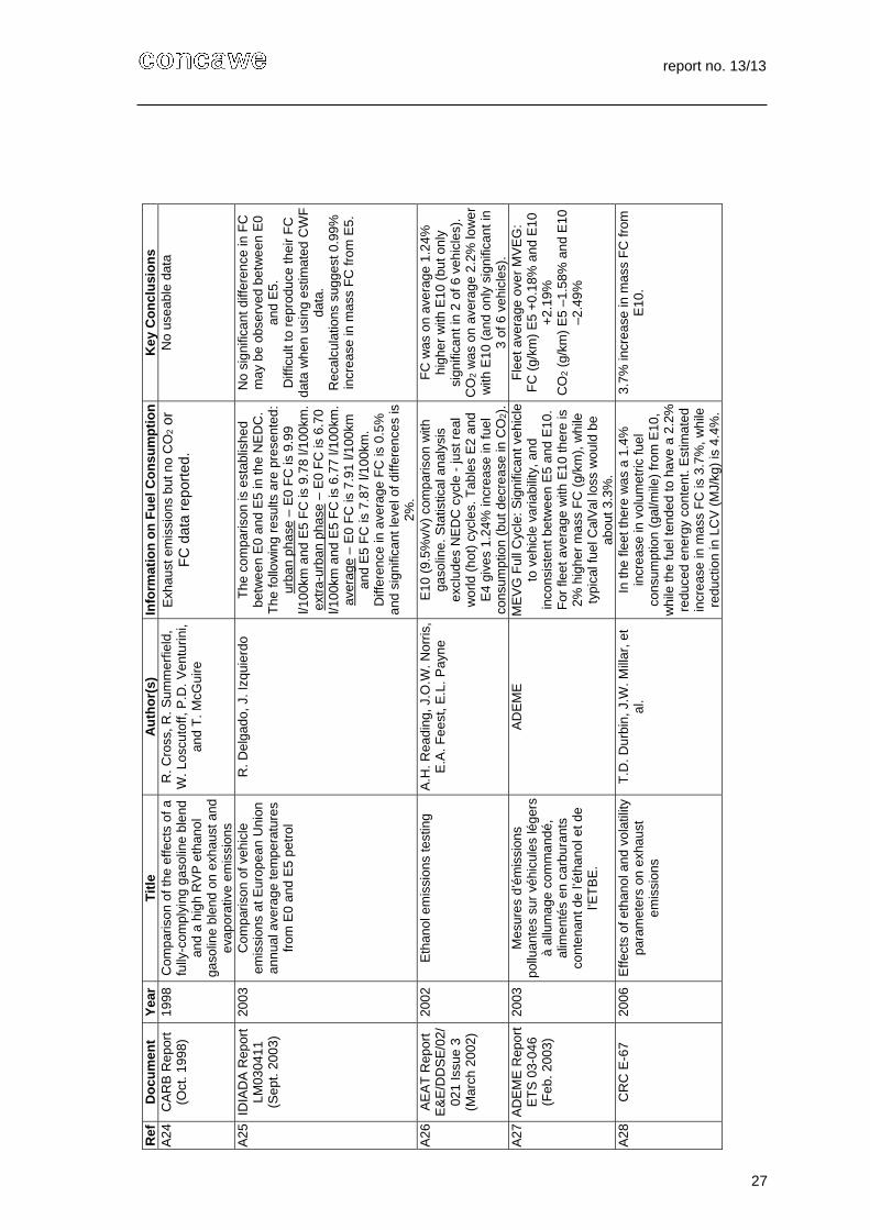
report no. 13/13

27

Ref

D

ocu

men

tY

ear

Tit

le

Au

tho

r(s)

Info

rmat

ion

on

Fu

el C

on

sum

pti

on

Key

Co

ncl

usi

on

sA

24

CA

RB

Re

port

(O

ct.

1998

) 19

98

Com

par

iso

n of

the

effe

cts

of a

fu

lly-c

omp

lyin

g g

asol

ine

ble

nd

and

a h

igh

RV

P e

than

ol

gaso

line

blen

d on

exh

aust

an

d ev

apor

ativ

e e

mis

sion

s

R. C

ross

, R. S

umm

erfie

ld,

W.

Losc

utof

f, P

.D.

Ven

turin

i, an

d T

. M

cGui

re

Exh

aust

em

issi

ons

but n

o C

O2 o

r F

C d

ata

repo

rted

. N

o us

eab

le d

ata

A25

ID

IAD

A R

epor

t LM

0304

11

(Sep

t. 20

03)

200

3C

omp

aris

on

of v

ehic

le

emis

sio

ns a

t Eur

opea

n U

nion

an

nua

l ave

rag

e te

mpe

ratu

res

from

E0

and

E5

petr

ol

R. D

elg

ado,

J. I

zqui

erdo

T

he c

ompa

riso

n is

est

ablis

hed

betw

een

E0

an

d E

5 in

the

NE

DC

. T

he fo

llow

ing

resu

lts a

re p

rese

nted

:ur

ban

phas

e –

E0

FC

is 9

.99

l/100

km a

nd E

5 F

C is

9.7

8 l/1

00km

.ex

tra-

urb

an p

has

e –

E0

FC

is 6

.70

l/100

km a

nd E

5 F

C is

6.7

7 l/1

00km

.av

era

ge –

E0

FC

is 7

.91

l/10

0km

an

d E

5 F

C is

7.8

7 l/1

00km

. D

iffer

ence

in a

vera

ge

FC

is 0

.5%

an

d si

gnifi

cant

leve

l of d

iffer

ence

s is

2%

.

No

sig

nific

ant

diff

eren

ce in

FC

m

ay

be

obse

rved

bet

we

en

E0

an

d E

5.

Diff

icul

t to

repr

oduc

e th

eir

FC

da

ta w

hen

usi

ng

estim

ated

CW

F

data

. R

ecal

cula

tions

sug

ges

t 0.9

9%

incr

ease

in m

ass

FC

from

E5.

A26

A

EA

T R

epor

t E

&E

/DD

SE

/02/

021

Issu

e 3

(Mar

ch 2

002

)

2002

Eth

anol

em

issi

ons

test

ing

A.H

. R

eadi

ng,

J.O

.W.

Nor

ris,

E.A

. F

eest

, E

.L.

Pay

ne

E10

(9.

5%v/

v) c

ompa

rison

with

ga

solin

e. S

tatis

tical

an

alys

is

excl

ude

s N

ED

C c

ycle

- ju

st r

eal

wo

rld (

hot

) cy

cles

. Tab

les

E2

and

E4

give

s 1.

24%

incr

ease

in f

uel

cons

umpt

ion

(but

dec

reas

e in

CO

2).

FC

was

on

ave

rage

1.2

4%

hig

her

with

E1

0 (b

ut o

nly

sign

ifica

nt in

2 o

f 6 v

ehic

les)

. C

O2 w

as o

n av

erag

e 2.

2% lo

we

r w

ith E

10 (

and

onl

y si

gnifi

cant

in

3 of

6 v

ehic

les)

. A

27 A

DE

ME

Rep

ort

ET

S 0

3-04

6 (F

eb. 2

003)

200

3M

esur

es d

’ém

issi

ons

pollu

ante

s su

r vé

hicu

les

lége

rs

à al

lum

age

com

man

dé,

al

ime

ntés

en

carb

uran

ts

cont

enan

t de

l’éth

anol

et d

e l’E

TB

E.

AD

EM

E

ME

VG

Ful

l Cyc

le: S

ign

ifica

nt v

ehic

le

to v

ehic

le v

aria

bilit

y, a

nd

inco

nsis

tent

be

twe

en E

5 a

nd E

10.

For

flee

t ave

rage

with

E1

0 th

ere

is

2% h

ighe

r m

ass

FC

(g/

km),

whi

le

typi

cal f

uel C

alV

al lo

ss w

oul

d be

ab

out

3.3

%.

Fle

et a

vera

ge o

ver

MV

EG

: F

C (

g/km

) E

5 +

0.18

% a

nd E

10

+2.

19%

C

O2 (

g/km

) E

5 –1

.58

% a

nd

E10

–2

.49

%

A28

C

RC

E-6

7

200

6E

ffect

s of

eth

anol

and

vo

latil

ity

para

met

ers

on e

xha

ust

emis

sion

s

T.D

. D

urbi

n, J

.W.

Mill

ar,

et

al.

In th

e fle

et th

ere

wa

s a

1.4%

in

crea

se in

vol

umet

ric fu

el

cons

umpt

ion

(gal

/mile

) fr

om E

10,

wh

ile th

e fu

el t

end

ed to

hav

e a

2.2%

re

duce

d e

nerg

y co

nten

t. E

stim

ated

in

cre

ase

in m

ass

FC

is 3

.7%

, wh

ile

redu

ctio

n in

LC

V (

MJ/

kg)

is 4

.4%

.

3.7%

incr

ease

in m

ass

FC

from

E

10.

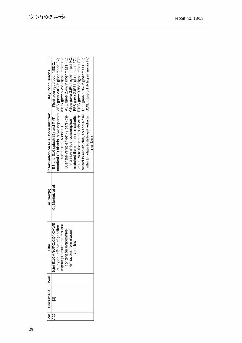
report no. 13/13

28

Ref

D

ocu

men

tY

ear

Tit

le

Au

tho

r(s)

Info

rmat

ion

on

Fu

el C

on

sum

pti

on

Key

Co

ncl

usi

on

sA

29

[3]

Jo

int E

UC

AR

/JR

C/C

ON

CA

WE

st

udy

on: e

ffect

s of

gas

olin

e va

pour

pre

ssur

e an

d et

han

ol

cont

ent o

n ev

apo

rativ

e em

issi

ons

from

mod

ern

vehi

cles

G. M

artin

i, et

al.

E5

and

E10

spl

ash

(S)

and

RV

P-

mat

ched

(E

) bl

ends

in t

wo

sepa

rate

ba

se fu

els

(A

and

B).

O

ver

the

vehi

cle

fleet

(7

cars

) th

e in

cre

ase

in fu

el c

onsu

mpt

ion

mat

ched

the

redu

ctio

n in

ca

lori

fic

valu

e. N

ote

that

not

all

fuel

s w

ere

test

ed in

all

vehi

cles

, so

som

e fu

el

effe

cts

rela

te to

diff

eren

t ve

hicl

e nu

mb

ers.

Fle

et a

vera

ged

ove

r N

ED

C:

A5S

gav

e 2.

8%

hig

her

mas

s F

C;

A10

S g

ave

5.2

% h

ighe

r m

ass

FC

;A

5E g

ave

2.4

% h

ighe

r m

ass

FC

;A

10E

gav

e 3.

9%

hig

her

mas

s F

C;

B5S

gav

e 2.

0%

hig

her

mas

s F

C;

B10

S g

ave

3.8

% h

ighe

r m

ass

FC

;B

5E g

ave

1.3

% h

ighe

r m

ass

FC

;B

10E

gav

e 3.

1%

hig

her

mas

s F

C

report no. 13/13

29

In addition to the reports listed in Appendix 1, data were also taken from the JRC/EUCAR/CONCAWE (JEC) study on the effects of ethanol content on evaporative emissions [3], which is also Report A29 in the above table. This study included emissions tests over the NEDC on seven test vehicles. Fuel consumption was calculated from carbon balance. Carbon weight fraction and calorific value were derived from GC analysis of each fuel. The fuel matrix consisted of two base fuels, A and B, and eight additional test fuels. Four of the additional fuels were blended from each base fuel, generating 5% and 10% ethanol blends, both as splash blends and as RVP-matched blends.

The overall conclusion from the FC data in this fleet of vehicles was that the increase in FC directly corresponded to the loss in calorific value, thus indicating no change in engine thermal efficiency. Interestingly, it was noted that the two base fuels had almost identical calorific values (42.805 MJ/kg and 42.812 MJ/kg) although they did not have the same fuel consumption. The difference in results between these two base fuels was vehicle dependent. This implies that there could be an influence of fuel properties other than ethanol (or oxygen) content on the measured FC, which prompted the investigation of other datasets – see Appendix 3.

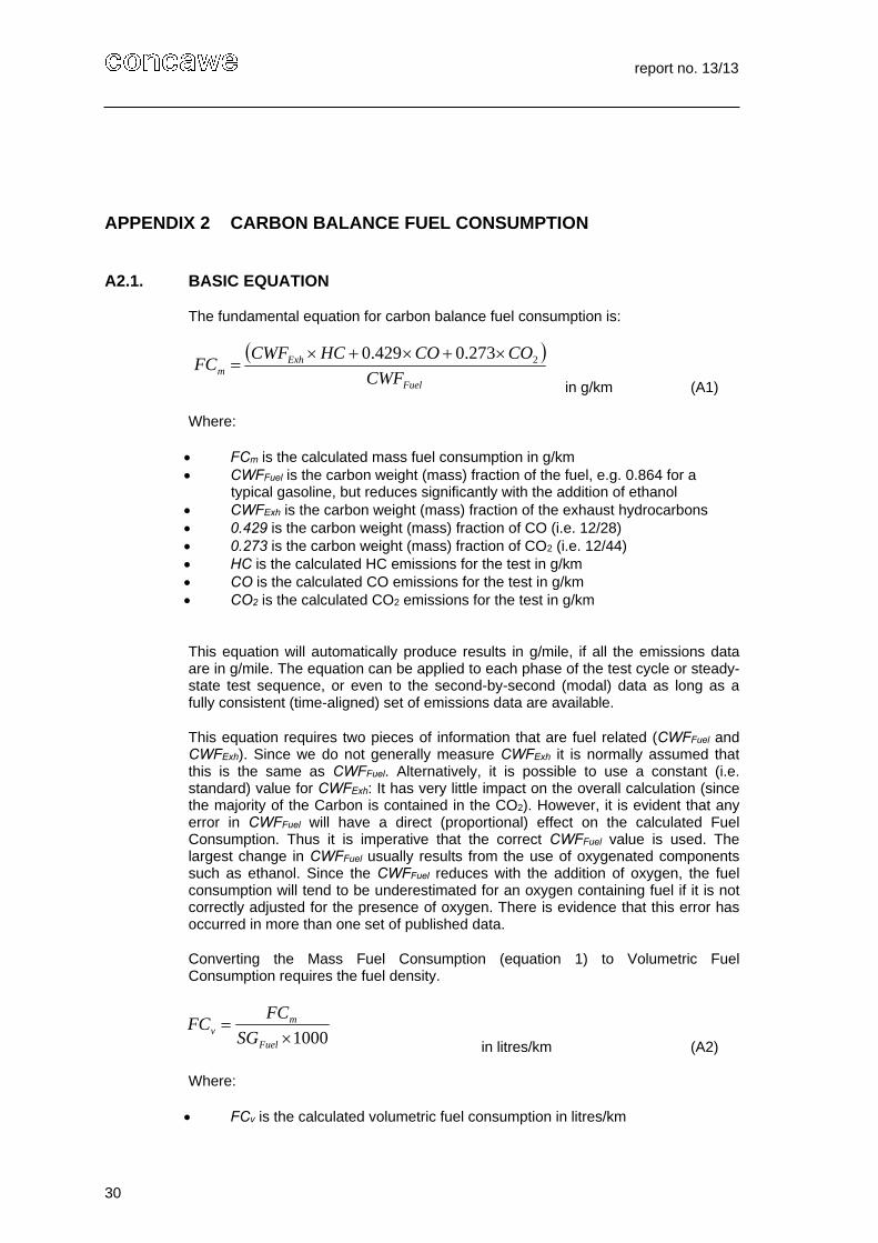
report no. 13/13

30

APPENDIX 2 CARBON BALANCE FUEL CONSUMPTION

A2.1. BASIC EQUATION

The fundamental equation for carbon balance fuel consumption is:

Fuel

Exhm CWF

COCOHCCWFFC 2273.0429.0

in g/km (A1)

Where:

FCm is the calculated mass fuel consumption in g/km CWFFuel is the carbon weight (mass) fraction of the fuel, e.g. 0.864 for a

typical gasoline, but reduces significantly with the addition of ethanol CWFExh is the carbon weight (mass) fraction of the exhaust hydrocarbons 0.429 is the carbon weight (mass) fraction of CO (i.e. 12/28) 0.273 is the carbon weight (mass) fraction of CO2 (i.e. 12/44) HC is the calculated HC emissions for the test in g/km CO is the calculated CO emissions for the test in g/km CO2 is the calculated CO2 emissions for the test in g/km

This equation will automatically produce results in g/mile, if all the emissions data are in g/mile. The equation can be applied to each phase of the test cycle or steady-state test sequence, or even to the second-by-second (modal) data as long as a fully consistent (time-aligned) set of emissions data are available.

This equation requires two pieces of information that are fuel related (CWFFuel and CWFExh). Since we do not generally measure CWFExh it is normally assumed that this is the same as CWFFuel. Alternatively, it is possible to use a constant (i.e. standard) value for CWFExh: It has very little impact on the overall calculation (since the majority of the Carbon is contained in the CO2). However, it is evident that any error in CWFFuel will have a direct (proportional) effect on the calculated Fuel Consumption. Thus it is imperative that the correct CWFFuel value is used. The largest change in CWFFuel usually results from the use of oxygenated components such as ethanol. Since the CWFFuel reduces with the addition of oxygen, the fuel consumption will tend to be underestimated for an oxygen containing fuel if it is not correctly adjusted for the presence of oxygen. There is evidence that this error has occurred in more than one set of published data.

Converting the Mass Fuel Consumption (equation 1) to Volumetric Fuel Consumption requires the fuel density.

1000

Fuel

mv SG

FCFC

in litres/km (A2)

Where:

FCv is the calculated volumetric fuel consumption in litres/km

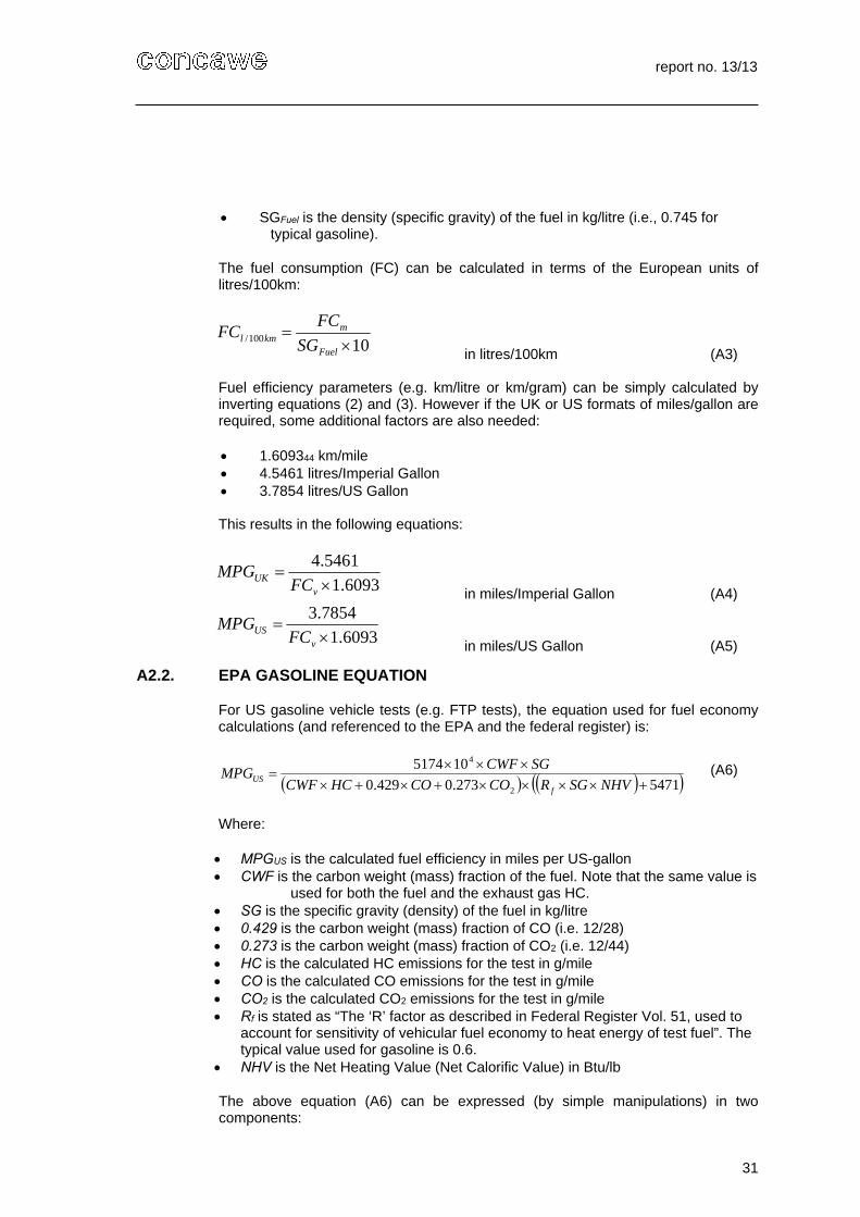
report no. 13/13

31

SGFuel is the density (specific gravity) of the fuel in kg/litre (i.e., 0.745 for typical gasoline).

The fuel consumption (FC) can be calculated in terms of the European units of litres/100km:

10100/

Fuel

mkml SG

FCFC

in litres/100km (A3)

Fuel efficiency parameters (e.g. km/litre or km/gram) can be simply calculated by inverting equations (2) and (3). However if the UK or US formats of miles/gallon are required, some additional factors are also needed:

1.609344 km/mile 4.5461 litres/Imperial Gallon 3.7854 litres/US Gallon

This results in the following equations:

6093.1

5461.4

vUK FC

MPG in miles/Imperial Gallon (A4)

6093.1

7854.3

vUS FC

MPG in miles/US Gallon (A5)

A2.2. EPA GASOLINE EQUATION

For US gasoline vehicle tests (e.g. FTP tests), the equation used for fuel economy calculations (and referenced to the EPA and the federal register) is:

5471273.0429.0

105174

2

4

NHVSGRCOCOHCCWF

SGCWFMPG

fUS

(A6)

Where:

MPGUS is the calculated fuel efficiency in miles per US-gallon CWF is the carbon weight (mass) fraction of the fuel. Note that the same value is

used for both the fuel and the exhaust gas HC. SG is the specific gravity (density) of the fuel in kg/litre 0.429 is the carbon weight (mass) fraction of CO (i.e. 12/28) 0.273 is the carbon weight (mass) fraction of CO2 (i.e. 12/44) HC is the calculated HC emissions for the test in g/mile CO is the calculated CO emissions for the test in g/mile CO2 is the calculated CO2 emissions for the test in g/mile Rf is stated as “The ‘R’ factor as described in Federal Register Vol. 51, used to

account for sensitivity of vehicular fuel economy to heat energy of test fuel”. The typical value used for gasoline is 0.6.

NHV is the Net Heating Value (Net Calorific Value) in Btu/lb

The above equation (A6) can be expressed (by simple manipulations) in two components:

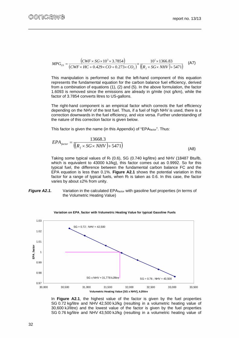
report no. 13/13

32

5471

83.136610

273.0429.0

7854.310 1

2

3

NHVSGRCOCOHCCWF

SGCWFMPG

fUS

(A7)

This manipulation is performed so that the left-hand component of this equation represents the fundamental equation for the carbon balance fuel efficiency, derived from a combination of equations (1), (2) and (5). In the above formulation, the factor 1.6093 is removed since the emissions are already in g/mile (not g/km), while the factor of 3.7854 converts litres to US-gallons.

The right-hand component is an empirical factor which corrects the fuel efficiency depending on the NHV of the test fuel. Thus, if a fuel of high NHV is used, there is a correction downwards in the fuel efficiency, and vice versa. Further understanding of the nature of this correction factor is given below.

This factor is given the name (in this Appendix) of “EPAfactor”. Thus:

5471

3.13668

NHVSGREPA

ffactor

(A8)

Taking some typical values of Rf (0.6), SG (0.740 kg/litre) and NHV (18487 Btu/lb, which is equivalent to 43000 kJ/kg), this factor comes out as 0.9992. So for this typical fuel, the difference between the fundamental carbon balance FC and the EPA equation is less than 0.1%. Figure A2.1 shows the potential variation in this factor for a range of typical fuels, when Rf is taken as 0.6. In this case, the factor varies by about ±2% from unity.

Figure A2.1. Variation in the calculated EPAfactor with gasoline fuel properties (in terms of the Volumetric Heating Value)

Variation on EPA_factor with Volumetric Heating Value for typical Gasoline Fuels

0.97

0.98

0.99

1

1.01

1.02

1.03

30,000 30,500 31,000 31,500 32,000 32,500 33,000 33,500

Volumetric Heating Value [SG x NHV], kJ/litre

EP

A_f

acto

r

SG = 0.72 ; NHV = 42,500

SG = 0.76 ; NHV = 43,500SG x NHV = 31,778 kJ/litre

In Figure A2.1, the highest value of the factor is given by the fuel properties SG 0.72 kg/litre and NHV 42,500 kJ/kg (resulting in a volumetric heating value of 30,600 kJ/litre) and the lowest value of the factor is given by the fuel properties SG 0.76 kg/litre and NHV 43,500 kJ/kg (resulting in a volumetric heating value of

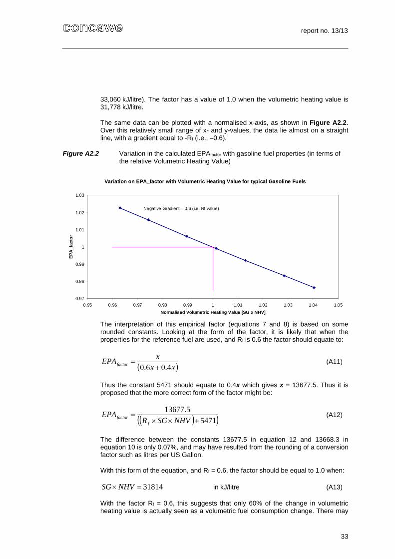
report no. 13/13

33

33,060 kJ/litre). The factor has a value of 1.0 when the volumetric heating value is 31,778 kJ/litre.

The same data can be plotted with a normalised x-axis, as shown in Figure A2.2. Over this relatively small range of x- and y-values, the data lie almost on a straight line, with a gradient equal to -Rf (i.e., –0.6).

Figure A2.2 Variation in the calculated EPAfactor with gasoline fuel properties (in terms of the relative Volumetric Heating Value)

Variation on EPA_factor with Volumetric Heating Value for typical Gasoline Fuels

0.97

0.98

0.99

1

1.01

1.02

1.03

0.95 0.96 0.97 0.98 0.99 1 1.01 1.02 1.03 1.04 1.05

Normalised Volumetric Heating Value [SG x NHV]

EP

A_f

acto

r

Negative Gradient = 0.6 (i.e. Rf value)

The interpretation of this empirical factor (equations 7 and 8) is based on some rounded constants. Looking at the form of the factor, it is likely that when the properties for the reference fuel are used, and Rf is 0.6 the factor should equate to:

xx

xEPAfactor 4.06.0

(A11)

Thus the constant 5471 should equate to 0.4x which gives x = 13677.5. Thus it is proposed that the more correct form of the factor might be:

5471

5.13677

NHVSGREPA

ffactor (A12)

The difference between the constants 13677.5 in equation 12 and 13668.3 in equation 10 is only 0.07%, and may have resulted from the rounding of a conversion factor such as litres per US Gallon.

With this form of the equation, and Rf = 0.6, the factor should be equal to 1.0 when:

31814NHVSG in kJ/litre (A13)

With the factor Rf = 0.6, this suggests that only 60% of the change in volumetric heating value is actually seen as a volumetric fuel consumption change. There may

report no. 13/13

34

be thermodynamic reasons why the other 40% of the change in volumetric heating value is lost within the engine operation, and may relate to correlated changes in the HC type which could affect octane and stoichiometric air/fuel ratio. If this factor has been defined experimentally on older US vehicles (prior to 1986), it is possible that this factor is not appropriate to current vehicle populations around the world.

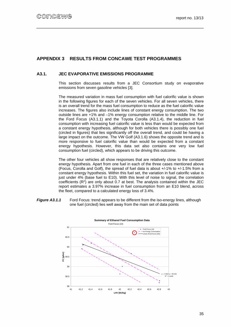
report no. 13/13

35

APPENDIX 3 RESULTS FROM CONCAWE TEST PROGRAMMES

A3.1. JEC EVAPORATIVE EMISSIONS PROGRAMME

This section discusses results from a JEC Consortium study on evaporative emissions from seven gasoline vehicles [3].

The measured variation in mass fuel consumption with fuel calorific value is shown in the following figures for each of the seven vehicles. For all seven vehicles, there is an overall trend for the mass fuel consumption to reduce as the fuel calorific value increases. The figures also include lines of constant energy consumption. The two outside lines are +1% and –1% energy consumption relative to the middle line. For the Ford Focus (A3.1.1) and the Toyota Corolla (A3.1.4), the reduction in fuel consumption with increasing fuel calorific value is less than would be expected from a constant energy hypothesis, although for both vehicles there is possibly one fuel (circled in figures) that lies significantly off the overall trend, and could be having a large impact on the outcome. The VW Golf (A3.1.6) shows the opposite trend and is more responsive to fuel calorific value than would be expected from a constant energy hypothesis. However, this data set also contains one very low fuel consumption fuel (circled), which appears to be driving this outcome.

The other four vehicles all show responses that are relatively close to the constant energy hypothesis. Apart from one fuel in each of the three cases mentioned above (Focus, Corolla and Golf), the spread of fuel data is about +/-1% to +/-1.5% from a constant energy hypothesis. Within this fuel set, the variation in fuel calorific value is just under 4% (base fuel to E10). With this level of noise to signal, the correlation coefficients (R2) are only about 0.7 at best. The analysis contained within the JEC report estimates a 3.97% increase in fuel consumption from an E10 blend, across the fleet, compared to a calculated energy loss of 3.4%.

Figure A3.1.1 Ford Focus: trend appears to be different from the iso-energy lines, although one fuel (circled) lies well away from the main set of data points

Summary of Ethanol Fuel Consumption Data

y = -0.9521x + 99.402

R2 = 0.4445

58

58.5

59

59.5

60

60.5

61

41 41.2 41.4 41.6 41.8 42 42.2 42.4 42.6 42.8 43

LHV [MJ/kg]

FC

[g

/km

]

Ford Focus (10)

Iso-Energy Consumption

Linear (Ford Focus (10))

Ford Focus (10)

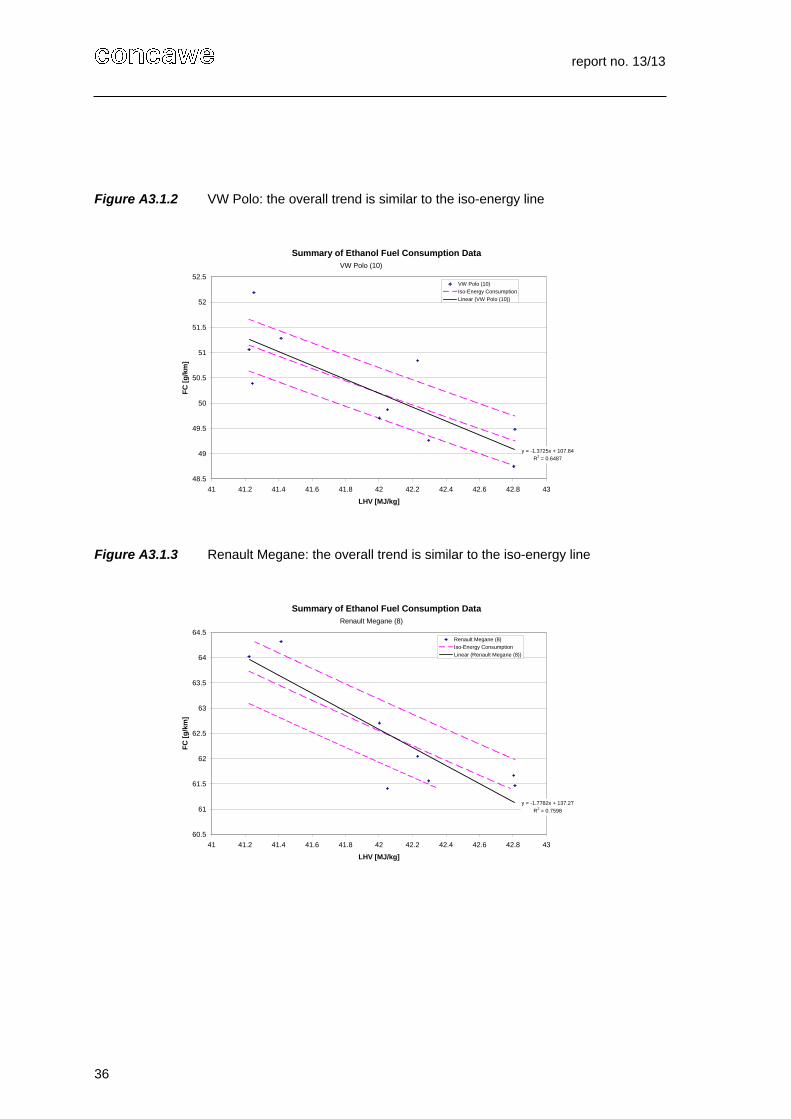
report no. 13/13

36

Figure A3.1.2 VW Polo: the overall trend is similar to the iso-energy line

Summary of Ethanol Fuel Consumption Data

y = -1.3725x + 107.84

R2 = 0.6487

48.5

49

49.5

50

50.5

51

51.5

52

52.5

41 41.2 41.4 41.6 41.8 42 42.2 42.4 42.6 42.8 43

LHV [MJ/kg]

FC

[g

/km

]

VW Polo (10)

Iso-Energy Consumption

Linear (VW Polo (10))

VW Polo (10)

Figure A3.1.3 Renault Megane: the overall trend is similar to the iso-energy line

Summary of Ethanol Fuel Consumption Data

y = -1.7782x + 137.27

R2 = 0.7598

60.5

61

61.5

62

62.5

63

63.5

64

64.5

41 41.2 41.4 41.6 41.8 42 42.2 42.4 42.6 42.8 43

LHV [MJ/kg]

FC

[g

/km

]

Renault Megane (8)

Iso-Energy Consumption

Linear (Renault Megane (8))

Renault Megane (8)

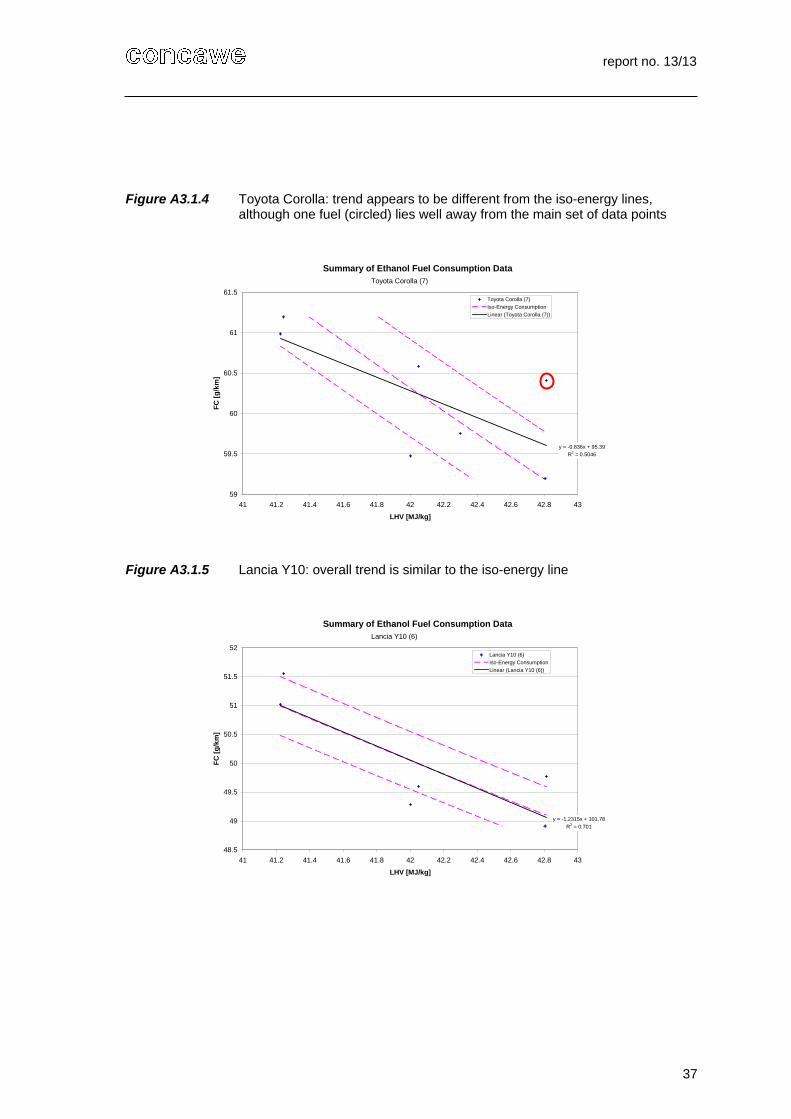
report no. 13/13

37

Figure A3.1.4 Toyota Corolla: trend appears to be different from the iso-energy lines, although one fuel (circled) lies well away from the main set of data points

Summary of Ethanol Fuel Consumption Data

y = -0.836x + 95.39

R2 = 0.5046

59

59.5

60

60.5

61

61.5

41 41.2 41.4 41.6 41.8 42 42.2 42.4 42.6 42.8 43

LHV [MJ/kg]

FC

[g

/km

]

Toyota Corolla (7)

Iso-Energy Consumption

Linear (Toyota Corolla (7))

Toyota Corolla (7)

Figure A3.1.5 Lancia Y10: overall trend is similar to the iso-energy line

Summary of Ethanol Fuel Consumption Data

y = -1.2315x + 101.78

R2 = 0.701

48.5

49

49.5

50

50.5

51

51.5

52

41 41.2 41.4 41.6 41.8 42 42.2 42.4 42.6 42.8 43

LHV [MJ/kg]

FC

[g

/km

]

Lancia Y10 (6)

Iso-Energy Consumption

Linear (Lancia Y10 (6))

Lancia Y10 (6)

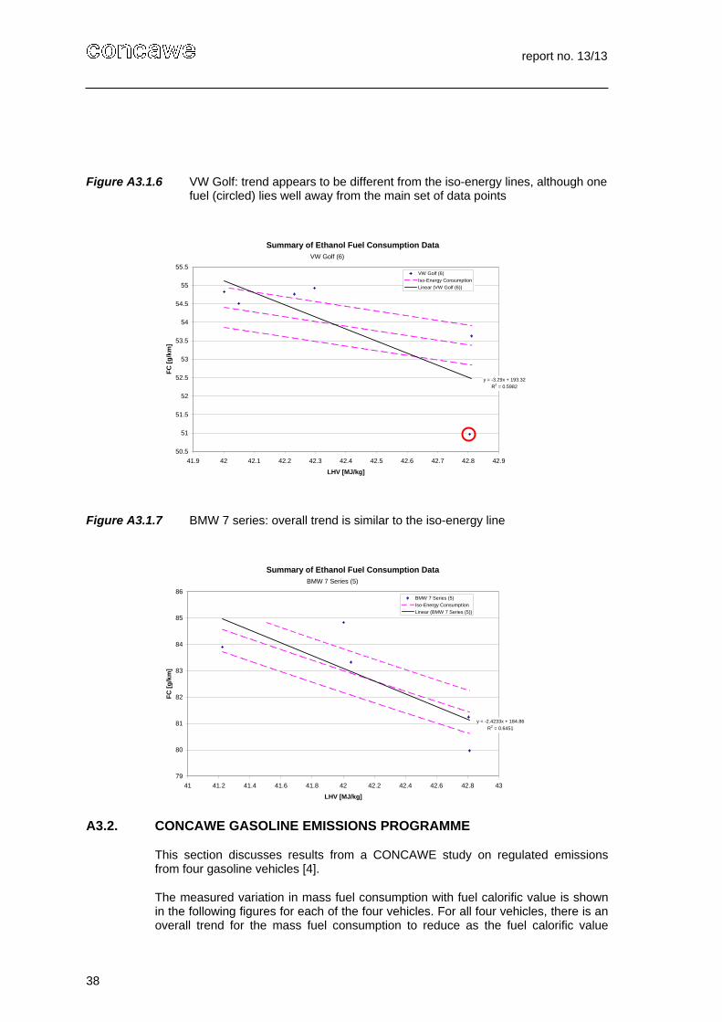
report no. 13/13

38

Figure A3.1.6 VW Golf: trend appears to be different from the iso-energy lines, although one fuel (circled) lies well away from the main set of data points

Summary of Ethanol Fuel Consumption Data

y = -3.29x + 193.32

R2 = 0.5982

50.5

51

51.5

52

52.5

53

53.5

54

54.5

55

55.5

41.9 42 42.1 42.2 42.3 42.4 42.5 42.6 42.7 42.8 42.9

LHV [MJ/kg]

FC

[g

/km

]

VW Golf (6)

Iso-Energy Consumption

Linear (VW Golf (6))

VW Golf (6)

Figure A3.1.7 BMW 7 series: overall trend is similar to the iso-energy line

Summary of Ethanol Fuel Consumption Data

y = -2.4233x + 184.86

R2 = 0.6451

79

80

81

82

83

84

85

86

41 41.2 41.4 41.6 41.8 42 42.2 42.4 42.6 42.8 43

LHV [MJ/kg]

FC

[g

/km

]

BMW 7 Series (5)

Iso-Energy Consumption

Linear (BMW 7 Series (5))

BMW 7 Series (5)

A3.2. CONCAWE GASOLINE EMISSIONS PROGRAMME

This section discusses results from a CONCAWE study on regulated emissions from four gasoline vehicles [4].

The measured variation in mass fuel consumption with fuel calorific value is shown in the following figures for each of the four vehicles. For all four vehicles, there is an overall trend for the mass fuel consumption to reduce as the fuel calorific value

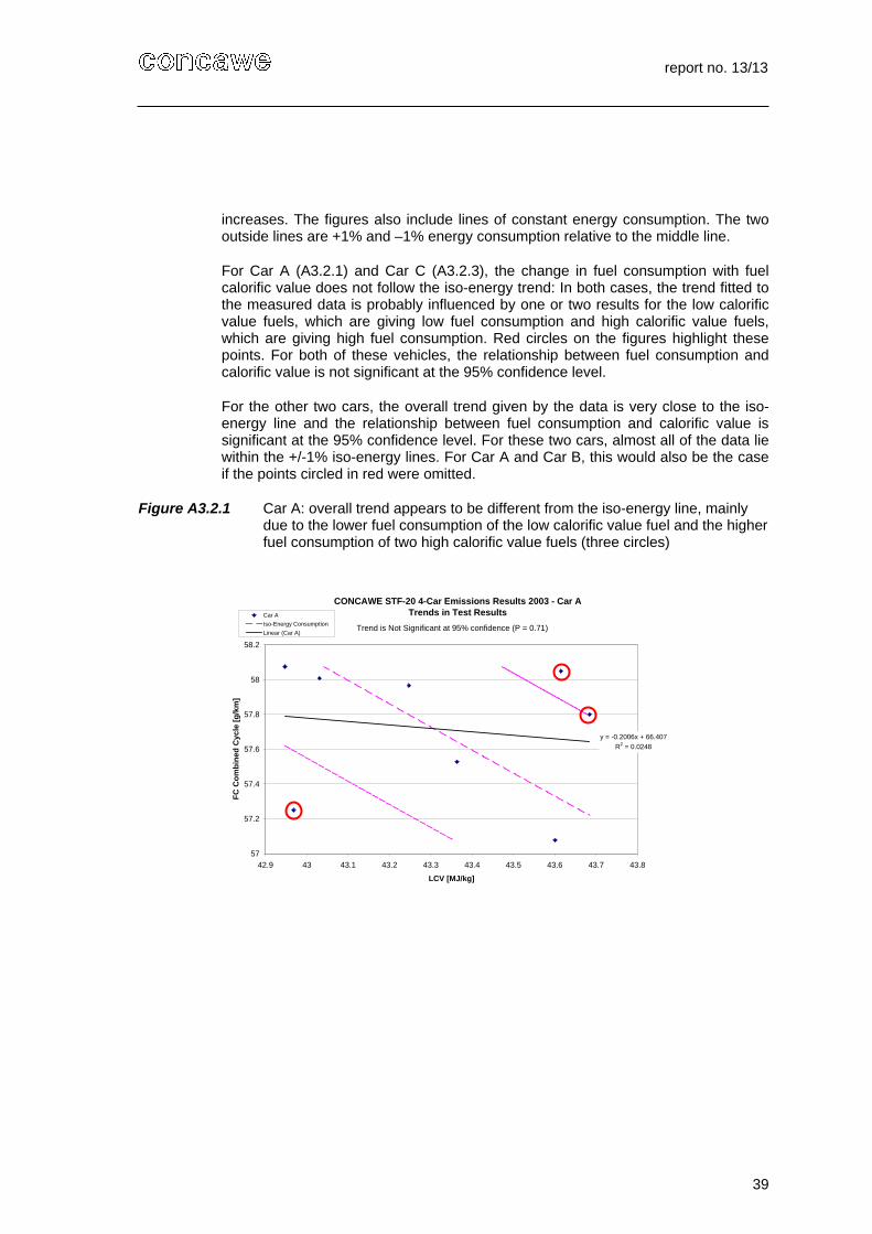
report no. 13/13

39

increases. The figures also include lines of constant energy consumption. The two outside lines are +1% and –1% energy consumption relative to the middle line.

For Car A (A3.2.1) and Car C (A3.2.3), the change in fuel consumption with fuel calorific value does not follow the iso-energy trend: In both cases, the trend fitted to the measured data is probably influenced by one or two results for the low calorific value fuels, which are giving low fuel consumption and high calorific value fuels, which are giving high fuel consumption. Red circles on the figures highlight these points. For both of these vehicles, the relationship between fuel consumption and calorific value is not significant at the 95% confidence level.

For the other two cars, the overall trend given by the data is very close to the iso-energy line and the relationship between fuel consumption and calorific value is significant at the 95% confidence level. For these two cars, almost all of the data lie within the +/-1% iso-energy lines. For Car A and Car B, this would also be the case if the points circled in red were omitted.

Figure A3.2.1 Car A: overall trend appears to be different from the iso-energy line, mainly due to the lower fuel consumption of the low calorific value fuel and the higher fuel consumption of two high calorific value fuels (three circles)

CONCAWE STF-20 4-Car Emissions Results 2003 - Car ATrends in Test Results

y = -0.2006x + 66.407

R2 = 0.0248

57

57.2

57.4

57.6

57.8

58

58.2

42.9 43 43.1 43.2 43.3 43.4 43.5 43.6 43.7 43.8

LCV [MJ/kg]

FC

Co

mb

ine

d C

ycle

[g

/km

]

Car A

Iso-Energy Consumption

Linear (Car A)Trend is Not Significant at 95% confidence (P = 0.71)

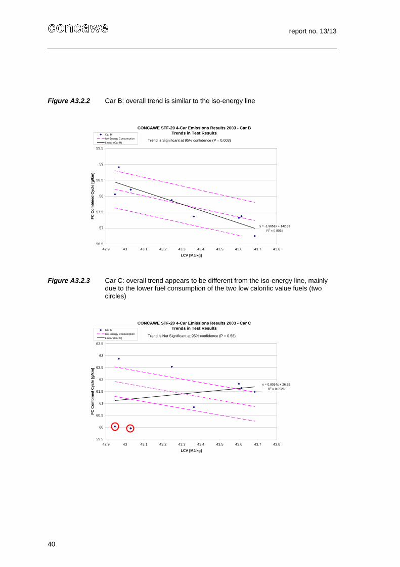
report no. 13/13

40

Figure A3.2.2 Car B: overall trend is similar to the iso-energy line

CONCAWE STF-20 4-Car Emissions Results 2003 - Car BTrends in Test Results

y = -1.9651x + 142.83

R2 = 0.8015

56.5

57

57.5

58

58.5

59

59.5

42.9 43 43.1 43.2 43.3 43.4 43.5 43.6 43.7 43.8

LCV [MJ/kg]

FC

Co

mb

ined

Cy

cle

[g

/km

]

Car B

Iso-Energy Consumption

Linear (Car B)Trend is Significant at 95% confidence (P = 0.003)

Figure A3.2.3 Car C: overall trend appears to be different from the iso-energy line, mainly

due to the lower fuel consumption of the two low calorific value fuels (two circles)

CONCAWE STF-20 4-Car Emissions Results 2003 - Car CTrends in Test Results

y = 0.8014x + 26.69

R2 = 0.0526

59.5

60

60.5

61

61.5

62

62.5

63

63.5

42.9 43 43.1 43.2 43.3 43.4 43.5 43.6 43.7 43.8

LCV [MJ/kg]

FC

Co

mb

ined

Cyc

le [

g/k

m]

Car C

Iso-Energy Consumption

Linear (Car C)Trend is Not Significant at 95% confidence (P = 0.58)

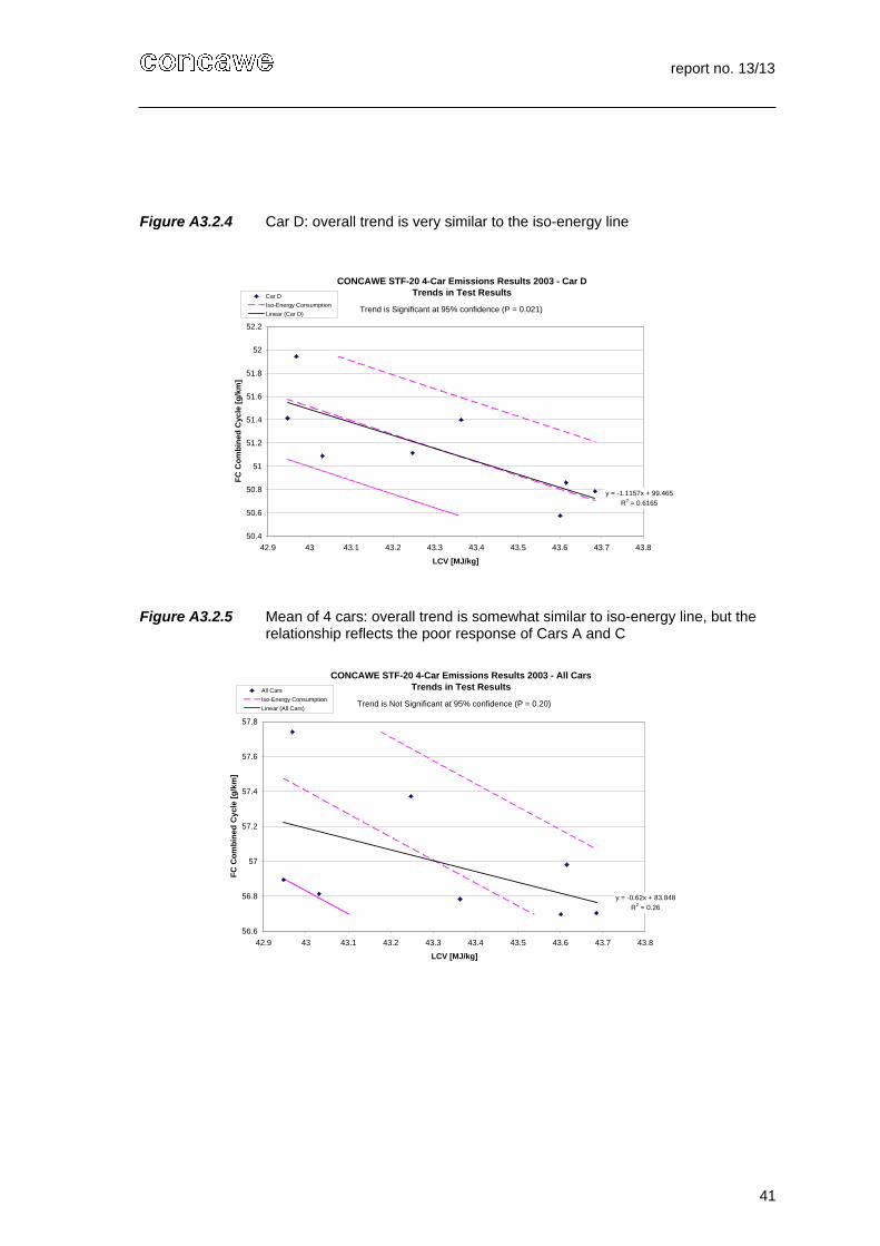
report no. 13/13

41

Figure A3.2.4 Car D: overall trend is very similar to the iso-energy line

CONCAWE STF-20 4-Car Emissions Results 2003 - Car DTrends in Test Results

y = -1.1157x + 99.465

R2 = 0.6165

50.4

50.6

50.8

51

51.2

51.4

51.6

51.8

52

52.2

42.9 43 43.1 43.2 43.3 43.4 43.5 43.6 43.7 43.8

LCV [MJ/kg]

FC

Co

mb

ined

Cyc

le [

g/k

m]

Car D

Iso-Energy Consumption

Linear (Car D)Trend is Significant at 95% confidence (P = 0.021)

Figure A3.2.5 Mean of 4 cars: overall trend is somewhat similar to iso-energy line, but the

relationship reflects the poor response of Cars A and C

CONCAWE STF-20 4-Car Emissions Results 2003 - All CarsTrends in Test Results

y = -0.62x + 83.848

R2 = 0.26

56.6

56.8

57

57.2

57.4

57.6

57.8

42.9 43 43.1 43.2 43.3 43.4 43.5 43.6 43.7 43.8

LCV [MJ/kg]

FC

Co

mb

ined

Cy

cle

[g/k

m]

All Cars

Iso-Energy Consumption

Linear (All Cars)Trend is Not Significant at 95% confidence (P = 0.20)

CONCAWE Boulevard du Souverain 165

B-1160 Brussels Belgium

Tel: +32-2-566 91 60 Fax: +32-2-566 91 81

e-mail: info@concawe.org website: http://www.concawe.org