1

Assessment of the Gaussian Covariance Approximation over an Earth-

Asteroid Encounter Period

By Daniel Mattern 1) 1)Omitron, Inc., Beltsville, MD | NASA Goddard Space Flight Center, Flight Dynamics Facility, Greenbelt, MD

In assessing the risk an asteroid may pose to the Earth, the asteroid’s state is often predicted for many years, often decades.

Only by accounting for the asteroid’s initial state uncertainty can a measure of the risk be calculated. With the asteroid’s state

uncertainty growing as a function of the initial velocity uncertainty, orbit velocity at the last state update, and the time from

the last update to the epoch of interest, the asteroid’s position uncertainties can grow to many times the size of the Earth when

propagated to the encounter “risk corridor.” This paper examines the merits of propagating the asteroid’s state covariance as

an analytical matrix. The results of this study help to bound the efficacy of applying different metrics for assessing the risk

an asteroid poses to the Earth. Additionally, this work identifies a criterion for when different covariance propagation methods

are needed to continue predictions after an Earth-encounter period.

Key Words: planetary defense, uncertainty characterization, asteroid

Nomenclature

𝑃𝐻𝐴

𝑇𝐶𝐴

𝑁𝐸𝐴

𝑃𝑐

𝐷𝑀𝐻

𝑆𝑂𝐼

𝑅𝑠𝑐

𝛼

𝐻

𝐷

𝜀

𝑣

𝑟

𝐺

𝑀

Δ

𝜎

𝐶𝑄𝐹

: potentially hazardous asteroid

: time of closest approach

: near-Earth asteroid

: probability of collision

: Mahalanobis distance

: sphere of influence

: characteristic scale ratio

: albedo

: absolute magnitude

: asteroid diameter

: orbit energy

: orbit velocity

: orbit radius

: gravitational constant

: mass of the central body

: finite difference

: standard deviation

: covariance quality factor

1. Introduction

Many metrics exist for assessing the risk a potential

hazardous asteroid (PHA) may pose to the Earth.† A

fundamental issue with any metric is generally the scale

of the asteroid’s position uncertainty when propagated to

the time of closest approach (TCA) with the Earth. As

PHAs generally have orbits somewhat similar to Earth,

their synodic period is often multi-year or even decades-

long. As such, any initial measurement uncertainty is

very large when propagated to TCA.

Two common metrics that are used to assess a

collision risk are the probability of collision (𝑃𝑐) and

Mahalanobis distance (𝐷𝑀𝐻).1,2) Large uncertainties

generally affect 𝑃𝑐 calculations by returning negligible

values early on and by returning false positives with

subsequent measurements (described later).

Mahalanobis distance calculations are affected by large

uncertainties predominantly based on how close the

distribution gets to the Earth’s gravitational sphere of

influence (SOI). Because 𝐷𝑀𝐻 calculations require the

uncertainty distribution to be approximated by a

covariance matrix, this matrix imposes Gaussian

assumptions on the distribution in the coordinate frame in

†PHAs are defined as near-Earth objects whose minimum orbit intersection distance with the Earth is 0.05 AU or less and

whose absolute magnitude is 22.0 or brighter.

https://ntrs.nasa.gov/search.jsp?R=20170003913 2018-06-08T15:45:44+00:00Z

2

which the matrix is represented.[2] These assumptions

are challenged when the distribution is propagated

through a significant gravitational gradient.

This paper examines the appropriate domains for

using 𝐷𝑀𝐻 or 𝑃𝑐 to assess an asteroid’s impact risk.

Often, the difficulty of calculating 𝑃𝑐 is the necessity to

use a large-scale Monte Carlo approximation of the

covariance matrix, which is computationally expensive

and often time-consuming. Conversely, 𝐷𝑀𝐻 can be

calculated by propagating the 6x6 position matrix using

a standard state-transition matrix. As such, this paper

identifies a criterion – called the characteristic scale ratio

(𝑅𝑠𝑐) – for determining which metric is more appropriate.

2. Background

2.1. Observability and Orbit Determination

While many small asteroids strike the Earth

frequently without serious consequence, the threat posed

by asteroids only tens of meters in size is non-trivial. In

2013, a 20-meter asteroid exploded roughly 30 km over

Chelyabinsk, Russia. The resulting shock wave damaged

nearly 7,200 buildings and injured over 1,500 people.

Current NEO population estimates predict there are

nearly 10 million NEOs larger than the Chelyabinsk

asteroid that are yet undiscovered.3) The Tunguska event

in 1908 flattened nearly 500,000 acres of forest in the

uninhabited area of the Eastern Siberian Taiga. That

asteroid was estimated to be roughly 40 meters in

diameter. A similarly sized, denser asteroid created a

nearly 1 mile wide crater in the Arizona desert 50,000

years ago. Current estimates of undiscovered NEOs

larger than 40 meters exceeds 300,000.3)

In 2005, the United States Congress directed a

survey to find 90% of all NEOs with diameters larger

than 140 meters by 2020. Such asteroids, were they to

impact Earth, would release more energy than the largest

nuclear weapon ever tested. As of 2017, only 28% of

asteroids larger than 140 meters have been discovered -

the primary detection difficulty stemming from the

limited observability of small celestial objects.3)

The estimated diameter of an asteroid is related to its

reflectivity (quantified through its albedo, 𝛼) and

brightness in the sky (quantified as the absolute

magnitude, 𝐻) through the following equation:

𝐷 =1329

√𝛼10−0.2𝐻 (1)

Measuring the reflectivity, or albedo, of an asteroid

generally requires an in-depth composition analysis best

performed in-situ. As such, the size of an asteroid is most

commonly estimated by its absolute magnitude alone,

with albedo approximated to be between 0.05 and 0.25

with an average of 0.1. Figure 1 below shows the

approximate size range of detectable asteroids with

absolute magnitudes between 20 and 25 (the lower limit

of detection for most current ground-based telescopes).

The number of telescopes that can detect dim objects

decreases with increasing magnitude, implying that there

are very few telescopes currently able to detect objects

with magnitudes above 21 – 22. This is why the

catalogue of asteroids larger than 140 m has remained so

limited.

The limited observability of these small asteroids

leads to additional problems – namely, large orbit

uncertainties following ground-based observation. With

the detectability of dim objects improving with proximity

to Earth, smaller objects are generally only observable

within narrow encounter windows – typically less than a

few days. Orbit determination is improved by observing

an appreciable section of an orbit period. With NEO

asteroids’ heliocentric periods often in the range of one

to three years, a few days’ worth of observations leads to

observing less than 1% of an asteroid’s orbit. While a

given asteroid’s position can be well determined with

such a limited observation arc, the resultant orbit energy

and velocity cannot.

Large initial orbit velocity uncertainties lead to poor

position predictions in the future. This can be seen by

propagating two states with an initially small difference

in velocity. From the equation for orbit energy,

𝜀 =𝑣2

2−

𝐺𝑀

𝑟 (2)

Figure 1: Approximate asteroid size as determined from absolute magnitude, H. Here, asteroid albedo is estimated to lie between 0.05 and 0.25.

3

and taking the derivative of energy with respect to orbit

velocity, one can see that orbit energy uncertainty is not

only related to initial velocity uncertainty but also the

orbit velocity at the time the uncertainty is found.

Δ𝜀 = 𝑣Δ𝑣 (3)

In other words, an orbit velocity uncertainty applied

at periapsis will result in a larger position uncertainty

compared to the same orbit uncertainty propagated from

apoapsis. Figure 2 below shows an example of this

difference. For this case, a heliocentric orbit with a 3.2-

year orbit period was used. This orbit had an aphelion

orbit velocity of about 10 km/s and a perihelion velocity

of about 40 km/s. Figure 2 shows the resultant position

uncertainty after one orbit with an uncertainty of only 10

cm/s applied at both orbit apses.

While this orbit is somewhat representative of the

family of PHAs currently catalogued, the achievable

velocity uncertainty is highly dependent on the number

of observations, the observation geometry, and a bevy of

other factors. As such, typical velocity uncertainties can

range widely from 5 to 10 cm/s up to 50 cm/s, resulting

in position error growths anywhere between 500 km to

65,000 kilometers per year.

2.2. Risk Assessment Metrics

The risk posed to the Earth by a near-Earth asteroid

(NEA) is often difficult to quantify. While simulations

of the damage caused by asteroids of various sizes and

composition are possible using atmospheric density

models and complex fluid dynamics software, assessing

the likelihood of a particular impact requires direct

observation of that asteroid along its orbit. Complicating

this problem is that the ability to detect asteroids that may

cause regional-level devastation is near the current limits

of telescopic detection. As such, many PHAs have

limited observations – leading to large orbit uncertainties.

Propagating these uncertainties, say to a potential Earth

impact, only causes the position uncertainty to grow, as

was shown in the previous section. Hence, when the

uncertainty contour is used to calculate the probability of

collision (𝑃𝑐), the 𝑃𝑐 value often comes back

insignificantly small because the Earth’s volume

subsumes so little of the uncertainty contour. Figure 3

shows the predicted position of the asteroid Apophis

propagated from shortly after its discovery to the first

possible Earth impact in 2029.

This initial risk assessment of Apophis yielded a

calculated 𝑃𝑐 of only 0.33%.4) Such a small value could

cause hesitancy if action were necessary. While it was

later determined that Apophis posed no threat to Earth (it

will still pass closer to Earth than many communication

satellites), this may not be the case for future discoveries.

One proposed improved metric for assessing risk was

proposed via the use of the Mahalanobis distance.5) This

calculation returns the number of standard deviations a

point is from the center of a distribution. One benefit of

this metric over 𝑃𝑐 is the exclusion of a phenomenon

referred to as “𝑃𝑐 roll-off.” This phenomenon is caused

as the covariance matrix – the measure of the orbit

uncertainty – collapses as a result of additional orbit

Figure 3: Image from NASA JPL Near Earth Object Program (neo.jpl.nasa.gov/news/news146.html)

Figure 2: Position uncertainty growth from intial velocity uncertainty of 10 cm/s

4

measurements. As such, the local probability density

temporarily rises in the vicinity of the Earth, causing the

𝑃𝑐 value to increase. In the Apophis case, additional

measurements caused the covariance matrix to collapse

close to the Earth, and the 𝑃𝑐 rose to 2.7%.4) Eventually,

additional observations caused the covariance to collapse

beyond the surface of the Earth, and the 𝑃𝑐 dropped to

effectively zero. Conversely, an initial Mahalanobis

distance calculation returns a 𝜎-contour which would

trend monotonically with subsequent measurements.

Following the Apophis example, the initial risk

assessment would have likely yielded 1𝜎 ≤ 𝐷𝑀𝐻 ≤ 2𝜎.

This can be interpreted as having between a 1 in 3 and 1

in 22 chance of an impact. Subsequent measurements

would have collapsed the covariance matrix, hence

returning something like 2𝜎 ≤ 𝐷𝑀𝐻 ≤ 3𝜎, or between 1

in 22 and 1 in 370 chance of impact. Compare this to the

increase of 𝑃𝑐 from 0.33% to 2.7% using the same

measurements.

3. Motivation and Approach

3.1. Propagating through Gravity Gradients

It was found in Ref. 5) that propagating the

covariance matrix through an Earth encounter period

using only the state transition matrix caused the matrix to

“teeter” or torque as it passed the Earth. As such, the

leading and trailing edges of the matrix were stretched

out and pivoted toward the Earth, causing the uncertainty

distribution to shift its principal axes in the heliocentric

frame from predominantly along-track prior to the

encounter to predominantly cross-track afterward. The

magnitude of the reorientation was dependent on two

main factors: 1) how close the nominal trajectory passed

by the Earth, and 2) how large the uncertainty distribution

was prior to entering the Earth’s SOI.5)

3.2. Miss Distances and Uncertainty Distributions

The reorientation of the covariance as it passed the

Earth motivated analysis to relate the reorientation to

Earth’s gravitational field. This analysis aimed to

compare the largest eigenvalue of the analytical

covariance matrix just prior to entering the Earth’s

gravitational SOI to the asteroid’s minimum nominal

miss distance with the Earth. The largest eigenvalue was

used because this represents the largest spatial dimension

of the uncertainty distribution. The minimum nominal

miss distance was used as it implicitly relates to the

largest gravitational magnitude that the distribution

would encounter throughout its trajectory. The ratio of

the eigenvalue and the minimum miss distance was in

turn called the characteristic scale ratio, or 𝑅𝑠𝑐.

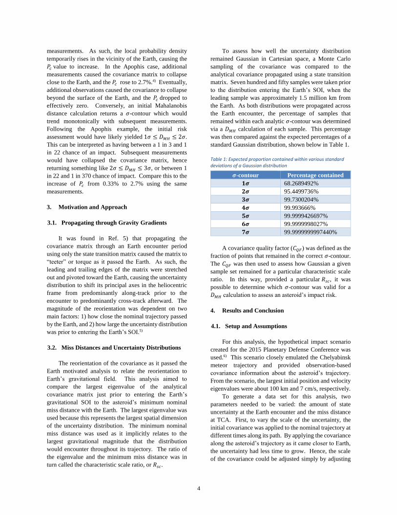
To assess how well the uncertainty distribution

remained Gaussian in Cartesian space, a Monte Carlo

sampling of the covariance was compared to the

analytical covariance propagated using a state transition

matrix. Seven hundred and fifty samples were taken prior

to the distribution entering the Earth’s SOI, when the

leading sample was approximately 1.5 million km from

the Earth. As both distributions were propagated across

the Earth encounter, the percentage of samples that

remained within each analytic 𝜎-contour was determined

via a 𝐷𝑀𝐻 calculation of each sample. This percentage

was then compared against the expected percentages of a

standard Gaussian distribution, shown below in Table 1.

Table 1: Expected proportion contained within various standard deviations of a Gaussian distribution

𝝈-contour Percentage contained

𝟏𝝈 68.2689492%

𝟐𝝈 95.4499736%

𝟑𝝈 99.7300204%

𝟒𝝈 99.993666%

𝟓𝝈 99.9999426697%

𝟔𝝈 99.9999998027%

𝟕𝝈 99.9999999997440%

A covariance quality factor (𝐶𝑄𝐹) was defined as the

fraction of points that remained in the correct 𝜎-contour.

The 𝐶𝑄𝐹 was then used to assess how Gaussian a given

sample set remained for a particular characteristic scale

ratio. In this way, provided a particular 𝑅𝑠𝑐, it was

possible to determine which 𝜎-contour was valid for a

𝐷𝑀𝐻 calculation to assess an asteroid’s impact risk.

4. Results and Conclusion

4.1. Setup and Assumptions

For this analysis, the hypothetical impact scenario

created for the 2015 Planetary Defense Conference was

used.6) This scenario closely emulated the Chelyabinsk

meteor trajectory and provided observation-based

covariance information about the asteroid’s trajectory.

From the scenario, the largest initial position and velocity

eigenvalues were about 100 km and 7 cm/s, respectively.

To generate a data set for this analysis, two

parameters needed to be varied: the amount of state

uncertainty at the Earth encounter and the miss distance

at TCA. First, to vary the scale of the uncertainty, the

initial covariance was applied to the nominal trajectory at

different times along its path. By applying the covariance

along the asteroid’s trajectory as it came closer to Earth,

the uncertainty had less time to grow. Hence, the scale

of the covariance could be adjusted simply by adjusting

5

how long it was propagated. Second, to tailor the

minimum nominal miss distance at TCA, small impulsive

velocity perturbations were applied to the asteroid’s orbit

at the time the initial covariance was applied. By

adjusting the magnitude of these velocity perturbations,

it was possible to affect different miss distances.

Generally, the greater the applied perturbation, the

greater the nominal miss distance. By repeating this

process at a number of different times along the asteroid’s

trajectory, it was possible to accumulate a representative

set of characteristic scale ratios.

4.2. Results

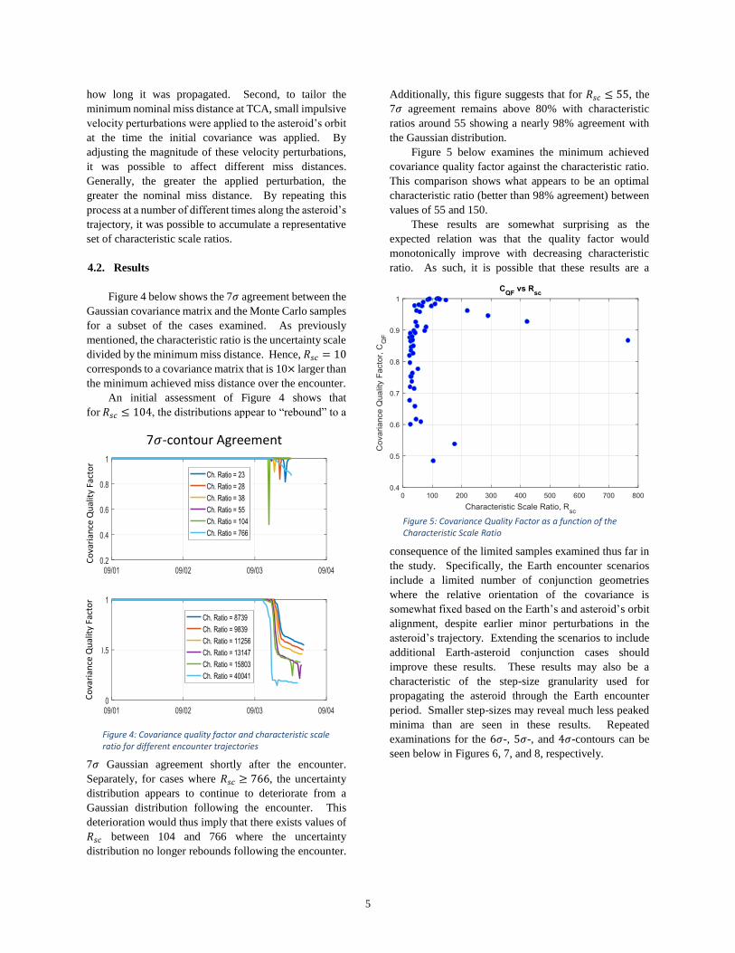
Figure 4 below shows the 7𝜎 agreement between the

Gaussian covariance matrix and the Monte Carlo samples

for a subset of the cases examined. As previously

mentioned, the characteristic ratio is the uncertainty scale

divided by the minimum miss distance. Hence, 𝑅𝑠𝑐 = 10

corresponds to a covariance matrix that is 10× larger than

the minimum achieved miss distance over the encounter.

An initial assessment of Figure 4 shows that

for 𝑅𝑠𝑐 ≤ 104, the distributions appear to “rebound” to a

7𝜎 Gaussian agreement shortly after the encounter.

Separately, for cases where 𝑅𝑠𝑐 ≥ 766, the uncertainty

distribution appears to continue to deteriorate from a

Gaussian distribution following the encounter. This

deterioration would thus imply that there exists values of

𝑅𝑠𝑐 between 104 and 766 where the uncertainty

distribution no longer rebounds following the encounter.

Additionally, this figure suggests that for 𝑅𝑠𝑐 ≤ 55, the

7𝜎 agreement remains above 80% with characteristic

ratios around 55 showing a nearly 98% agreement with

the Gaussian distribution.

Figure 5 below examines the minimum achieved

covariance quality factor against the characteristic ratio.

This comparison shows what appears to be an optimal

characteristic ratio (better than 98% agreement) between

values of 55 and 150.

These results are somewhat surprising as the

expected relation was that the quality factor would

monotonically improve with decreasing characteristic

ratio. As such, it is possible that these results are a

consequence of the limited samples examined thus far in

the study. Specifically, the Earth encounter scenarios

include a limited number of conjunction geometries

where the relative orientation of the covariance is

somewhat fixed based on the Earth’s and asteroid’s orbit

alignment, despite earlier minor perturbations in the

asteroid’s trajectory. Extending the scenarios to include

additional Earth-asteroid conjunction cases should

improve these results. These results may also be a

characteristic of the step-size granularity used for

propagating the asteroid through the Earth encounter

period. Smaller step-sizes may reveal much less peaked

minima than are seen in these results. Repeated

examinations for the 6𝜎-, 5𝜎-, and 4𝜎-contours can be

seen below in Figures 6, 7, and 8, respectively.

Co

vari

ance

Qu

alit

y Fa

cto

r C

ova

rian

ce Q

ual

ity

Fact

or

Figure 4: Covariance quality factor and characteristic scale ratio for different encounter trajectories

7𝜎-contour Agreement

Figure 5: Covariance Quality Factor as a function of the Characteristic Scale Ratio

6

6𝜎-contour Agreement

Figure 6: Covariance quality factor trending with time across Earth TCA (left) and minimum quality factor as a function of characteristic ratio (right)

5𝜎-contour Agreement

Figure 7: Covariance quality factor trending with time across Earth TCA (left) and minimum quality factor as a function of characteristic ratio (right)

4𝜎-contour Agreement

Figure 8: Covariance quality factor trending with time across Earth TCA (left) and minimum quality factor as a function of characteristic ratio (right)

7

As expected, these figures show that the quality degrades

with decreasing 𝜎-contours, implying that the

distribution becomes less Gaussian closer to the nominal

value. This result advocates a lower limit of around

5𝜎 when using a Mahalanobis metric for quantifying the

impact risk of an asteroid, based on at least a 95%

agreement with the Gaussian distribution.

5. Conclusions and Future Work

Preliminary results from this analysis suggest that

𝐷𝑀𝐻 calculations are a well suited risk metric for cases

where 𝑅𝑠𝑐 ≤ 150. However, this analysis also suggests

that 𝐷𝑀𝐻 values below 5𝜎 are poorly representative of a

Gaussian distribution. This can be seen qualitatively in

Figures 9 and 10 below. In both figures, the top plot

shows the 1-dimensional distance distribution between

the Monte Carlo samples and Earth; the bottom plot

shows the Monte Carlo samples of the covariance in the

heliocentric, Cartesian frame. For a 3-dimensional,

spatial Gaussian distribution, the corresponding distance

distribution is also Gaussian for cases where the mean is

much greater than the standard deviation (𝜇 ≫ 𝜎).

Hence, the top plot is very informative for how Gaussian

the distribution remains after encountering the Earth.

Both figures show the distributions a little more than two

weeks after encountering Earth, and an obvious tail can

be seen in the histogram in Figure 10 – implying a poor

Gaussian approximation for smaller 𝜎-contours. For

such cases where the uncertainty distribution does not

remain Gaussian, a metric like 𝑃𝑐 would still likely be

necessary.

Future work is still needed to address the peaked

minima shown in Figures 4, 6, 7, and 8. As stated

previously, the sharp peaks are likely due to the step-size

granularity during the Earth encounter period. Repeating

the propagations with smaller step-sizes should rectify

this issue. Additional asteroid trajectories will also need

to be examined for this work to be complete. These

trajectories will need to include a variety of relative

velocity angles to capture different covariance

orientations as the uncertainty distribution crosses

through the Earth’s gravitational field.

References 1) Akella, M. and Alfriend, K.: Probability of Collision

Between Space Objects, Journal of Guidance, Control,

and Dynamics, Vol. 23, No. 5, September-October

2000

2) Mahalanobis, P. C.: On the generalized distance in

statistics, Proceedings of the National Institute of

Sciences of India, Vol. 2, No. 1, pp. 49-55, 1936

Figure 9: Distance distribution (top) and 3-dimensional position uncertainty (bottom)

Figure 10: Distance distribution (top) and 3-dimensional position uncertainty (bottom)

8

3) US National Science and Technology Council: National

Near-Earth Object Preparedness Strategy, December

2016

4) Giorgini, J. D., et al: Predicting the Earth encounters of

(99942) Apophis,

neo.jpl.nasa.gov/apophis/Apophis_PUBLISHED_PAP

ER.pdf, October 2008

5) Mattern, D.: Deflection of an Earth-bound Asteroid

using a Gravity-assisted Kinetic Impactor, 2016

Astrodynamics Specialist Conference, September 2016

6) National Aeronautics and Space Administration Near

Earth Object Program: The 2015 PDC Hypothetical

Asteroid Impact Scenario, April 2015