Aouissi Jalel, Benabdallah Sihem,

Lili Chabaâne Zohra, Cudennec Christophe

Assessment of SWAT Potential Evapotranspiration Options and data-dependence for Estimating Actual

Evapotranspiration and Streamflow

2011 International SWAT Conference Toledo, Spain

June 15-17, 2011

« Modeling hydrology and diffuse pollution loads to assess surface water quality for a Tunisian agricultural catchment »

The relation between agriculture and water quality is recognized since 1970’s. This relation constitutes today an important goal in preserving water resources stored in dams. Risks of water contamination by nitrogen represents a main research field. Preserving water requires a better understanding of the processes governing the agricultural pressure and environmental impacts. The main objective of our study is to evaluate the impact of the real agriculture practices on the water quality at the catchment scale and to evaluate the fluxes of nitrogen going into the downstream dam using SWAT model.

Introduction (presentation included in my PhD project)

2

The accurate estimation of water loss by ET is very important for assessing water availability.

SWAT model uses Potential Evapotrtanspiration (PET), soil proprieties and land use characteristic for estimating actual evapotranspiration.

SWAT model offers the possibility of using several methods for computing the potential evapotranspiration methods including: (i) Penman-Montheith (PM), (ii) Hargreaves (H) and (iii) Priestly-Taylor (PT).

The PM model that requires five daily climatic parameters: temperature, solar radiation, wind speed and vapour pressure.

The first objective is to test the weather generator included in SWAT model for estimating missing climatic data and to evaluate the PM method for calculating PET with measured climatic data and with generated climatic data.

The second objective is to compare the use of the different ET models on daily and monthly PET, AET and Streamflow (Q) production

Purpose of This study

3

The Ichkeul National Park inscribed in the UNESCO world heritage wetland. It is in northern Tunisia, some 50 km north of the capital, Tunis.

Douimis

Melah wadi

Ghezala wadi

Tine wadi

Ichkeul

Joumine wadi

It is linked by a narrow

channel (Tinja channal) to

the lagoon of bizerte with

inturn has an outlet to the

Mediterranean sea.

Study area Location

4

Sejnane wadi

Lake Ichkeul

Lake Bizerte

Tinja Channel

Watershed of Joumine Dam

5

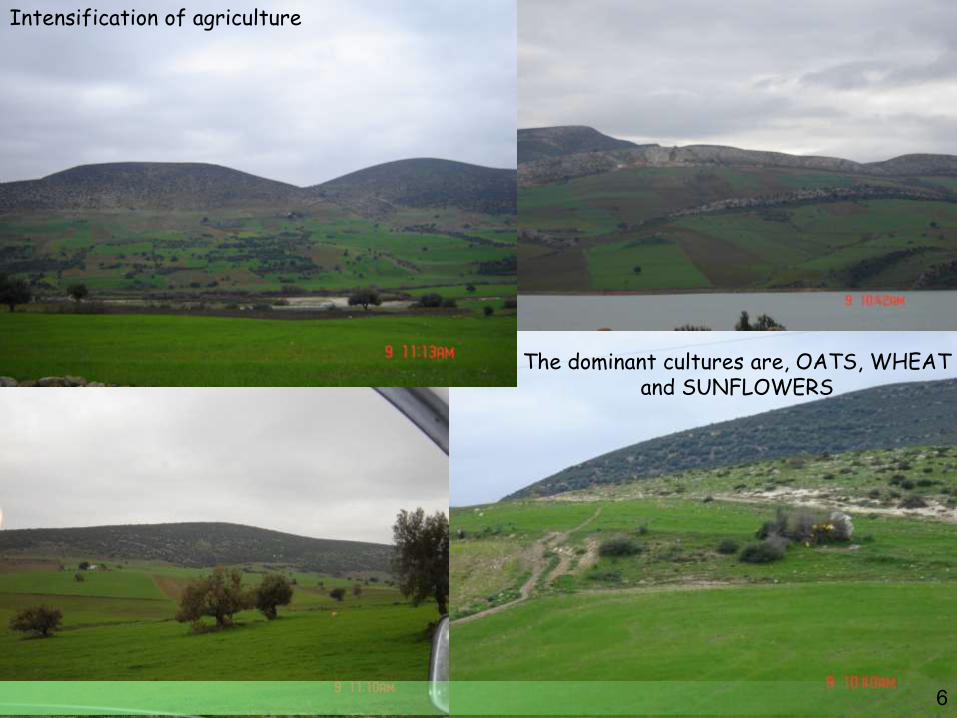
The dominant cultures are, OATS, WHEAT and SUNFLOWERS

Intensification of agriculture

6

Specific discharge (mm/year) Precipitation (mm/year) Evaporation (mm/year)

182 750 1629

7

Water is for drinking and irrigation

Agriculture practices

SWAT

Digital Elevation Model (DEM)

Channel Network

Model Outputs

Ponds Characteristic Climatic data(Rain, Tmax,

Tmin, Hr, Ray, Ws)

Soil map and soil

profiles properties

Land use Map

Streamflow, AET,MES, NO3-,

NH+, NO2- and PO4

3-.

Model Inputs and Outputs data

8

Digital elevation model

Land use / cover map

Soil map and properties profiles

Spatial data base

9

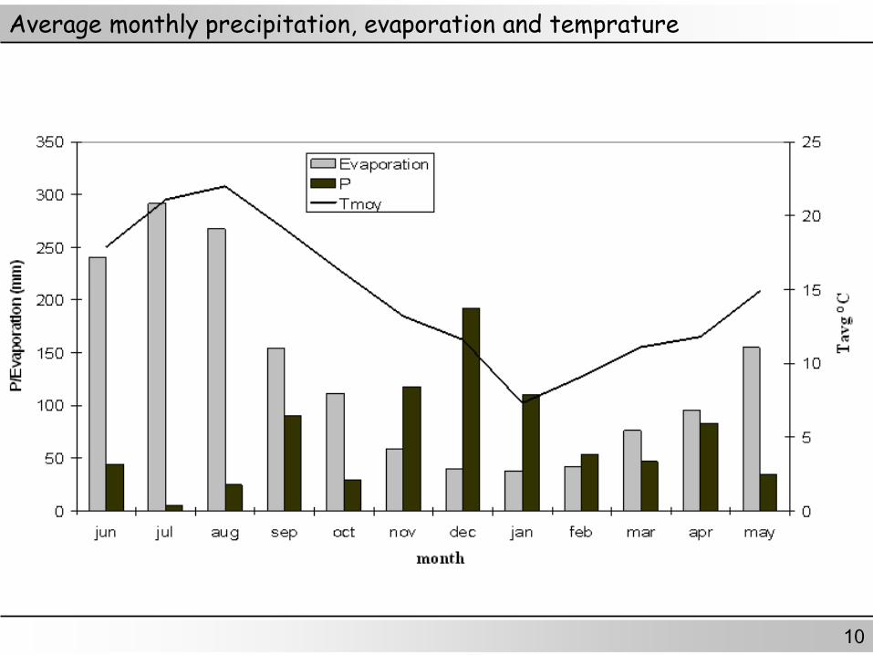
Average monthly precipitation, evaporation and temprature

10

Evaluation of Penman - Monteith method for calculating

potential evapoatranspiration with measured climatic data

and with those generated for SWAT-Predicted model actual

evapotranspiration and Streamflow.

Nash (EFF), coefficient of determination (R²), for relationship between daily SWAT Predicted potential evpotraspiration (PET), actual evapotranspiration (ET) and stream flow (Q) using Penman-Monteith method for estimating potential evapotranspiration considering all weather data and missing data: -U=without wind speed, -R=without solar radiation, -T= without temperature.

Used PET (measured climatic data) reference

PET PET (P, R, T, U) (-U) (-U,-T) (-U,-R,-T) (-R,-U) (-T,-R) (-T) (-R)

Nash 0.91 0.86 0.78 0.8 0.89 0.93 0.92

R² 0.91 0.86 0.84 0.86 0.9 0.94 0.95

Used ET (measured climatic data) reference

ET ET (P,R,T, U) (-U) (-U,-T) (-U,-R,-T) (-R,-U) (-T,-R) (-T) (-R)

Nash 0.92 0.78 0.65 0.99 0.73 0.85 0.84

R² 0.92 0.8 0.7 0.57 0.77 0.87 0.86

Used Q (measured climatic data) reference

Q Q (P, R, T, U) (-U) (-U,-T) (-U,-R,-T) (-R,-U) (-T,-R) (-T) (-R)

Nash 0.99 0.99 0.98 0.97 0.99 0.99 0.99

R² 0.99 0.99 0.99 0.99 0.99 0.99 0.99

Results Comparison for daily model runs

12

**indicated the comparison of simulated streamflow with measured data and those with generated data with observed streamflow.

Used PET (measured climatic data) reference

PET PET (P, R, T, U) (-U) (-U,-T) (-U,-R,-T) (-R,-U) (-T,-R) (-T) (-R)

Nash 0.98 0.97 0.9 0.88 0.96 0.98 0.94

R² 0.99 0.99 0.99 0.99 0.99 0.99 0.99

Used AET (measured climatic data) reference

ET ET (P,R,T, U) (-U) (-U,-T) (-U,-R,-T) (-R,-U) (-T,-R) (-T) (-R)

Nash 0.99 0.93 0.93 0.97 0.94 0.94 0.98

R2 0.99 0.94 0.94 0.97 0.94 0.94 0.98

Used Q (measured climatic data) reference

Q Q (P, R, T, U) (-U) (-U,-T) (-U,-R,-T) (-R,-U) (-T,-R) (-T) (-R)

Nash 0.99 0.99 0.99 0.99 0.99 0.99 0.99

R² 0.99 0.99 0.99 0.99 0.99 0.99 0.99

Used observed streamflow reference

Q Q (P, R, T, U) (-U) (-U,-T) (-U,-R,-T) (-R,-U) (-T,-R) (-T) (-R)

Nash 0.76** 0.757 0.77 0.74 0.72 0.74 0.77 0.73

R² 0.88** 0.88 0.88 0.88 0.87 0.88 0.88 0.88

Results Comparison for monthly model runs

13

0

5

10

15

20

25

30

35

40

Jan-9

0

Jan-9

1

Jan-9

2

Jan-9

3

Jan-9

4

Jan-9

5

Jan-9

6

Jan-9

7

Jan-9

8

Jan-9

9

Jan-0

0

Jan-0

1

Jan-0

2

Jan-0

3

Month

Str

ea

mfl

ow

(m

3s

-1)

Qobs Q(P,R,T,U) Q(-U) Q(-U,-T) Q(-U,-R,-T) Q(-R,-U) Q(-T,-R) Q(-T) Q(-R)

Comparison of the monthly observed streamflow with the simulated values based on measured as well as on generated weather data

14

SWAT - Predicting PET, ET and Streamflow using Penman -

Monteith, Hargreaves and Priestly Taylor methods for

estimating potential evapotranspiration

Used Simulated Potential evpotranspiration (PM) reference

PET(PM) PET (H) PET(PT)

Nash 0.66 0.72

RMSE (mm) 1.5 1.37

R2 0.74 0.77

Used Simulated Actual evpotranspiration (PM) reference

ET (PM) ET(H) ET(PT)

Nash 0.64 0.64

RMSE (mm) 0.43 0.43

R2 0.7 0.7

Used Simulated Streamflow (PM) reference

Q(PM) Q(H) Q(PT)

Nash 0.99 0.99

RMSE (m3s-1) 0.42 0.85

R2 0.99 0.99

Results Comparison for daily model runs

16

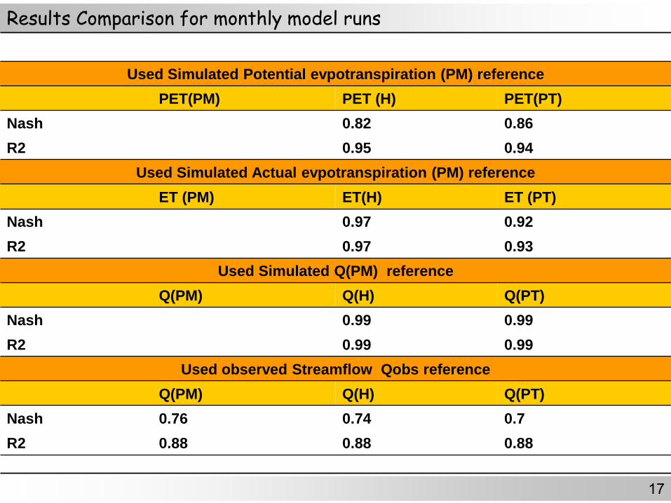
Used Simulated Potential evpotranspiration (PM) reference

PET(PM) PET (H) PET(PT)

Nash 0.82 0.86

R2 0.95 0.94

Used Simulated Actual evpotranspiration (PM) reference

ET (PM) ET(H) ET (PT)

Nash 0.97 0.92

R2 0.97 0.93

Used Simulated Q(PM) reference

Q(PM) Q(H) Q(PT)

Nash 0.99 0.99

R2 0.99 0.99

Used observed Streamflow Qobs reference

Q(PM) Q(H) Q(PT)

Nash 0.76 0.74 0.7

R2 0.88 0.88 0.88

Results Comparison for monthly model runs

17

Streamflow

0

5

10

15

20

25

30

35

40

Jan-

90

Jan-

91

Jan-

92

Jan-

93

Jan-

94

Jan-

95

Jan-

96

Jan-

97

Jan-

98

Jan-

99

Jan-

00

Jan-

01

Jan-

02

Jan-

03

Month

Str

ea

mfl

ow

(m

3s

-1)

Qobs Q(PM) Q(H) Q(PT)

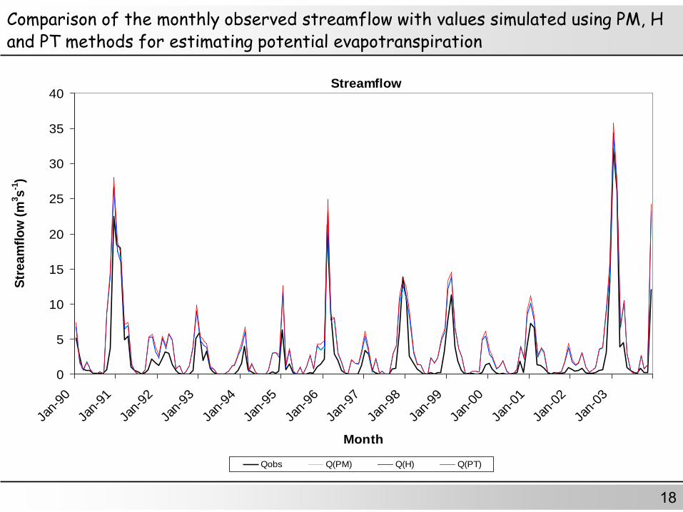
Comparison of the monthly observed streamflow with values simulated using PM, H and PT methods for estimating potential evapotranspiration

18

Sensitivity analysis and autocalibration of SWAT model

Sensitivity analysis (SA)

Latin Hypercube (LH)-One-factor-At time (OAT)

A parameters SA provides insights on which parameters contribute most the output variance.

The SA was performed for 16 parameters of hydrology that are related to streamflow (Q).

The parameters for calibration were selected by the SA results (the red parameters)

19

Paramètres rang

Alpha_Bf 1

Cn2 2

Ch_K2 3

Ch_N2 4

Esco 5

Sol_Z 6

Sol_Awc 7

Slope 8

Sol_K 9

Rchrg_Dp 10

Surlag 11

Epco 12

Gwqmn 13

Gw_Delay 14

Gw_Revap 15

Revapmn 16

20

Results of autocalibration of SWAT model

0

5

10

15

20

25

30

35

40

Jan-

90

Jan-

91

Jan-

92

Jan-

93

Jan-

94

Jan-

95

Jan-

96

Jan-

97

Jan-

98

Jan-

99

Jan-

00

Jan-

01

Jan-

02

Jan-

03

Jan-

04

Jan-

05

Jan-

06

mois

débit (

m3s

-1)

Qsim avant calibration Qsim aprés calibration Qobs

Str

eam

flow

(m

3s

-1)

Month

before after

R2 =0.95, Nash=0.88

The results show that the generated data did reproduce acceptably well the computations of PET passed on the Penman-Monteith method. However, using generation procedures to replace missing climatic data had an impact on daily actual evpotranspiration simulations. Daily and monthly streamflow modeling results showed a good similarity between those computed based on generated data and those with measured data from a local climatic station.

The advantage of generating climatic data based PET methods is to provide an option to estimate these variables when the weather stations do not have full dataset. The alternative ET methods (PM, H, PT) integrated in SWAT model for estimating PET showed a low influence in monthly streamflow and, actual evpotranspiration simulations.

21

Conclusion

Thank you for your attention

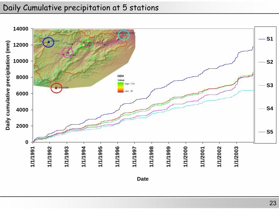
Daily Cumulative precipitation at 5 stations

0

2000

4000

6000

8000

10000

12000

140001

/1/1

99

1

1/1

/19

92

1/1

/19

93

1/1

/19

94

1/1

/19

95

1/1

/19

96

1/1

/19

97

1/1

/19

98

1/1

/19

99

1/1

/20

00

1/1

/20

01

1/1

/20

02

1/1

/20

03

Date

Da

ily

cu

mu

lati

ve

pre

cip

ita

tio

n (

mm

) S1

S2

S3

S4

S5

23

In the winter, the oueds that drain its hillside basin bring

down large amounts of fresh water and thus drown the

marshes and increase the level of the water in Lake Ichkeul.

In the summer, the water level drops as the oueds dry up

and intense evaporation takes place, resulting in increased

salinity. This drop in the water level sucks in salt water from

the Bizerte Lake via Oued Tinja.

It is this double seasonal alternation between a high water

level with low salinity and a low water level with high salinity,

that gives the Ichkeul ecosystems their originality.

Lak Ichkeul 24