ASSESSMENT OF NUMERICAL METHODS FOR LOWPRESSURE TURBINE TONE NOISE PREDICTION

L Pinelli1 ndash D Torzo2 ndash F Poli1 ndash A Arnone1

1Department of Industrial EngineeringUniversity of Florence Florence Italy

LorenzoPinelliarnonedeunifiit

2Avio SpA RampDRivalta di Torino Italy

DavideTorzoaviogroupcom

ABSTRACTThe capability to accurately predict the tone noise of Low Pressure Turbines (LPT) is cru-cial in designing and optimizing aircraft engine turbofans for low noise emissions Especiallyduring approach conditions the LPT is an important noise source for commercial aircraft Inthis paper two methodologies for exhaust turbine tone noise analysis are described and vali-dated against an experimental database measured in an acoustic test rig The first method apreliminary analysis technique is suitable during the early design phase whereas the secondmethodology is based on a 3D linearized approach which is used in the last steps of the acousticdesign Very good agreement is observed between numerical predictions and measurements forall interactions at approach operating conditions

NOMENCLATUREk harmonic or scattering index

K kernel elementkx ky axial and circumferential wavenumbersm circumferential orderN number of bladesNp number of panelsp disturbance acoustic pressureW acoustic powerR radiust time

L W loading and upwash elementsU V axial and circumferential components

of the mean flow velocityu v axial and circumferential components

of the disturbance velocityW mean velocity magnitudex y axial and circumferential coordinatesz chordwise coordinate

GreekΓ vortex strength per chord unit lengthΩ rotational speedω radian frequency ρ mean and disturbance densityθ stagger angle

Subscripts123 updownstream pressure vorticity (b)456 updownstream pressure vorticity (a)789 updownstream pressure vorticity (c)abc upstream inter-rows and downstream

fs first row second rowAcronymsPWL sound PoWer Level

= 10 log10(WW0) W0 = 1 pWSPL Sound Pressure Level

= 20 log10(p rmsp0) p0 = 20microPaV B vane blade

INTRODUCTIONNowadays strict legislation on airplane acoustic emissions imposes well defined limits of per-

ceived noise Such targets can be achieved through an accurate acoustic design and prediction of thewhole engine This procedure includes the analysis of the tonal noise generated inside the turbineas this component may play an important role in the overall engine acoustic signature at certain op-erating conditions For these reasons the development of fast and reliable numerical techniques tobe used both in the preliminary design phase and in the detailed assessments is strongly pushed bythe aeronautical industry Obviously different design phases require different kinds of tools fast and

1

Proceedings of

10th European Conference on Turbomachinery Fluid dynamics amp Thermodynamics

ETC10 April 15-19 2013 Lappeenranta Finland

OPEN ACCESS

Downloaded from wwweuroturboeu Copyright copy by the Authors

robust techniques for the preliminary choices accurate and reliable methods for the advanced designverification

Over the past four decades countless methods have been developed to predict the acoustic emis-sion at blade passing frequencies The first major contribution to the aeroacoustics of turbomachinerycan be attributed to Tyler and Sofrin (1962) who determined the link between blade count and ductmodes and their propagation behavior (cut-on or cut-off) Early methods to compute the strength ofthese spinning modes were based on analytic models derived from flat plate theory (Amiet (1974)Koch (1971)) where the sound emissions mainly depend on the difference between the wave angleand the stagger angle of the flat plate Then Ventres et al (1982) proposed a method which linked a2D flat plate theory for the unsteady aerodynamics to the acoustic modes of the actual 3D annular ductby means of strip analysis Other methods can be found in the literature Kaji and Okazaki (1970)developed a coupled statorrotor theory which however limited the analysis to a single frequency anddid not include the swirl effect On the contrary the methodology provided by Heinig (1983) maybe applied to turbomachines with non-uniform swirling flows A more accurate 3D analytical modelis presented by Posson et al (2010) Since the 1990s thanks to the growth in computer technologyldquotime-linearizedrdquo methods have been developed capable of dealing with real blade geometries andnon-uniform mean flows (Hall and Clark (1993) Hall and Lorence (1993) Chassaing and Gerolymos(2000) Campobasso and Giles (2003) Kennepohl et al (2001)) Such methods were first employedto evaluate the acoustic response of a single blade row but can also be efficiently used to predict thetone noise emission at the turbine exit by integrating the time-linearized code in a proper propagationprocedure (Korte et al (2005) Pinelli et al (2011a) Frey et al (2012))

In this paper two different approaches for tonal noise evaluation of a low pressure turbine willbe presented The first one a preliminary analysis technique is suitable for the early design phasewhereas the other one a 3D linearized method can be used in the last steps of the acoustic design

The preliminary acoustic tool is able to quickly estimate the tone noise emissions of a multistageLPT The method is based on simple mean line aerodynamic data and takes into account both acousticgeneration and propagation phenomena For this reason it can be seen as an extension of Hansonrsquoscoupled 2D cascade theory (Hanson (1994)) it extends Hansonrsquos theory for a single fan stage (tworows) to a multi-stage system (turbine) Adjacent blade rows are modeled as 2D flat plate cascadesand are included in a fully coupled unsteady analysis which satisfies the flow tangency boundarycondition on both rows simultaneously for several harmonics In this way noise generation scatteringand reflections are accounted for by solving a large linear system Further the swirling flow betweenadjacent rows is considered by means of actuator disks Following this approach the method de-scribes the evolution of the turbine-generated acoustic modes along the machine and provides foreach of them SPL and PWL values at the exhaust section

On the other hand the linearized method already described by the authors in previous works(Arnone et al (2003) Poli et al (2006) Boncinelli et al (2006) Poli et al (2009)) is based on afully three-dimensional aeroacoustic solver integrated in a proper propagation strategy (Pinelli et al(2011ba)) and can be fruitfully used during the detailed acoustic design

A wide validation of both tools is reported based on the experimental database measured in anacoustic test rig representative of the last stages of a low-pressure turbine All these activities arecarried out in the context of a research project on turbomachinery Computational Aeroelasticity (CA)and Computational Aeroacoustics (CAA) at the Department of Industrial Engineering (University ofFlorence) in collaboration with Avio SpA

THEORY OF THE NOISE PREDICTION METHODSThis section describes the theoretical basis of the two numerical methods which will be used to

predict acoustic emissions of a LPT for aeronautical applications Special emphasis will be put on the

2

preliminary analysis tool based on a semi-analytical method the 3D linearized method will be onlybriefly presented as it has already been described by the authors in (Pinelli et al (2011a))

Preliminary analysis toolThe preliminary analysis tool (named TNT Tone Noise Tool) is an extension of Hansonrsquos coupled

cascade theory from fan to LPT applications although it is acknowledged that the flat plate assump-tion is stronger for a turbine environment than for a fanOGV interaction Moreover the methodextension allows the analysis not only of the tone noise generation as did the original theory butalso of the acoustic propagation through successive rows up to turbine exhaust The tool which wasdeveloped computes the interaction between two adjacent blade rows (see right side of figure 1) andestimates either the effect of the wake from the upstream blade rows impinging on the successiveblade row (generation module) or the effect of an acoustic wave imposed in the gap between rows(propagation module) These interactions produce unsteady loading on both rows and thereby gener-ate outgoing acoustic waves The model takes into account reflectiontransmission characteristics andthe swirling flow between the two rows by means of actuator disk theory Unlike simpler methods inwhich there is a one-to-one relationship between wake harmonics and noise harmonics the presentedmethod simultaneously couples the effects of multiple harmonics in a large linear system In thisway noise generation scattering and reflections effects can be included in the model The solutionof the linear system is the unsteady loading distribution on both rows for each harmonic caused byincoming perturbations Once the unsteady loading is computed it is simple to derive the resultingoutput waves in terms of SPL and PWL

Basic theoryThe basis of Hansonrsquos coupled 2D theory is Smithrsquos theory (Smith (1973)) Smith derived a theo-

retical approach which relates the unsteady loading of a single cascade of flat plates with a specifiedvelocity disturbance entering the system This approach is based on an integral equation for the up-wash velocity (disturbance velocity component normal to the blade chord see left side of figure 1)on the cascade caused by the unknown load distribution The resulting equations can be solved for

0 xs xe

sf

ss

cf cs

x

y

θs

ΩfR ΩsR

1st row 2nd row

uimp

vimp

wake(generationmodule)

acoustic wave

(propagationmodule)

zs

zf

Smiths theory extended Hansons theory

0

y

VW

U

cu

v

unsteadyvelocity

v

u

vcosθ-usinθw

upwashvelocity

meanvelocity

θ x

zs

Figure 1 Geometry of Smithrsquos theory (left) and geometry of coupled cascade (right)

the loads and hence the outgoing acoustic waves can be evaluated As usual in acoustics Smith startswith the linearized differential equations for continuity and momentum and assumes the following

3

form for velocity and pressure perturbations (complex quantities are marked with the oversign ˜)uvp

= lte

uvp

e (kxx + kyy + ωt)

where ky =m

R(1)

This analysis leads to two families of solutions of the continuity and momentum equations the firstfamily includes the pressure waves which propagate updownstream (with or without attenuation)at the speed of sound a while the second one contains the vorticity waves which are convecteddownstream by the mean flow The respective axial wave numbers are given by

kx 12 =U(ω + V ky)plusmn a

radic(ω + V ky)2 minus (a2 minus U2)k2y

a2 minus U2kx 3 = minus(ω + V ky)

U(2)

Moreover the relations between velocity and pressure complex mode amplitudes are

u12 = kx 12v12ky

p12 = minus(ω + Ukx 12 + V ky)v12ky

and u3 = minuskyv3kx 3

(3)

Smith then deduces equation 4 which describes the total circumferential perturbation velocity relatedto each wave type

v(total)123 =

int c

0

lte

infinsum

k=minusinfin

vprime123 e(kx 123x + kyy + ωt) eminus(kx 123 cos θ + ky sin θ)z

Γ(z)

sdz (4)

Upstream of the cascade there will be only the v(total)1 component which corresponds to the circumfer-

ential velocity perturbation due to all upstream running pressure waves In the same way anywheredownstream of the row v(total)

2 (sum of downstream running pressure waves) and v(total)3 (sum of vortic-

ity waves) will be present Expressions for vprime1 vprime2 and vprime3 are directly derived from Smithrsquos theory (seeSmith (1973)) and respectively represent the influence of a unit loading element on the updownstreamrunning pressure and vorticity waves Then the load distribution over the blade chord is discretizedinto Np identical panels and the integral is converted to a sum according to

1

c

int zj+∆z2

zjminus∆z2

Γ(z)

Wdz =rArr L (j) where ∆z =

c

Np

(5)

Following Hansonrsquos approach equation 4 can thus be generalized for each row with multiple harmon-ics for any wave type

v(total) =W

sc

+infinsumk fs=minusinfin

Npsumi=1

lte

+infinsum

k sf=minusinfin

vprime e(kxx+ kyy+ωt) eminus(kx cos θ+ ky sin θ)zi

timesL (k fs i) (6)

Wave systemThe next step is to derive the form of all the waves which can result from a generic interaction

between adjacent rows for both generation and propagation cases When dealing with a wave genera-tion phenomenon the classical Tyler and Sofrin spinning modes are generated Such modes form thewave system for the generation module and are described in the fixed reference frame in the left sideof equations 7

m = ksNs minus kfNf

ω = kfNfΩf minus ksNsΩs︸ ︷︷ ︸(generation module)

m = m0 + kfNf + ksNs

ω = ω0 minus kfNfΩf minus ksNsΩs︸ ︷︷ ︸(propagation module)

(7)

4

The present extension of Hansonrsquos theory also allows the propagation of a single mode through suc-cessive rows (one at a time together with the previously analyzed row) This means that the wavesystem describing the propagation problem is different and has to be composed of the imposed wave(with m0 and ω0) together with all the scattering modes due to the two blade rows The wave sys-tem for the propagation module is depicted by the right side of equations 7 The same conclusionwas drawn by Hall et al (2006) in their work on flutter in a multistage environment Furthermoreif the imposed wave (with m0 and ω0) is a vector of turbulence modes right side of equations 7 alsodescribe the set of permitted broadband modes (see Hanson (2001))

Reflection and transmission coefficientsSwirling flow between rows must be considered in order to have a better representation of the

mean flow properties As explained in Hanson (1994) actuator disks can be used to turn the meanflow at the 1st row leading edge and at the 2nd row trailing edge (see figure 2) As the mean flowchanges across the inlet and exit interfaces the unsteady quantities vary as well This can be handledby employing reflection R and transmission T coefficients for all the waves Such coefficients aredirectly derived from the linearized continuity of mass and momentum

1st rowinlet disk

2nd rowexit disk

ρaaaMxa

ρcacMxc

ρbab

Mxb

Ms

v1v2

v3v4v1

v3

v8

v9

v1

v2

v8

v9

T1↦4 R1↦2

R1↦3

R2↦1T2↦8

T2↦9

R3↦1T3↦8

T3↦9

region b(inter-row)

region c(downstream)

region a(upstream)

0 xex

0 xex

1st rowleading edge

2nd rowtrailing edge

(RW1)f

(RW2)f

(RW3)f

(RW1)s

(RW2)s

(RW3)s

Ls

(DW1)s (DW2)s

(DW3)s

Lf

(DW1)f (DW2)f

(DW3)f

Rx↦yreflection coefficient

(from the incident wave x to the

reflected wave y)

Tx↦ytransmission coefficient

(from the wave x to the transmitted

wave y)

RW reflected wave

DW direct wave

Figure 2 Coupled theory reflectiontransmission coefficients (left) waves system (right)

Coupled 2D theoryIn order to couple the problem it is sufficient to construct the wave field between the 1st row

leading edge and the 2nd row trailing edge by means of direct waves coming from each loading element(via Smithrsquos formulae) plus the waves reflected from the inlet and exit interfaces (see figure 2) For aloading element of the 1st row for instance the direct waves (DW123)f from each panel are obtainedby Smithrsquos theory while the reflected waves (RW123)f can be built as follows

(RW1)f = [(DW2)f + (RW2)f]R2rarr1 + [(DW3)f + (RW3)f]R3rarr1

(RW2)f = [(DW1)f + (RW1)f]R1rarr2

(RW3)f = [(DW1)f + (RW1)f]R1rarr3

(8)

5

and similar equations hold for the 2nd row Such coupling equations are written in terms of transversevelocity v123 components Now the axial velocity u123 can be obtained by using equation 3 so thatit is straightforward to derive the upwash velocity (see Hanson (1994)) Together all the couplingequations (such as equations 6 and 8) written in terms of upwash velocity define four sub-matricesof influence and sub-matrices can be assembled into a large matrix representing the entire coupledsystem[

Kfrarrf Ksrarrf

Kfrarrs Ksrarrs

]times[Lf

Ls

]=

[Wf

Ws

](9)

When dealing with the propagation module of the acoustic tool the deeper structure of the coupledlinear system for the special case of minus1 lt kfs lt +1 becomes as shown in equation 10Inside this large system each sub-matrix includes the kernel quantity for each element discretizing thetwo rows It is worth noting how the system explicitly shows the modal and frequency scattering andhow it allows the inclusion of multiple reflections between the rows

Kfrarrfkf = minus1ks = minus1

0

0

Ksrarrfkf = minus1ks = minus1

Ksrarrfkf = 0ks = minus1

Ksrarrfkf = +1ks = minus1

0

Kfrarrfkf = 0ks = 0

0

Ksrarrfkf = minus1ks = 0

Ksrarrfkf = 0ks = 0

Ksrarrfkf = +1ks = 0

0

0

Kfrarrfkf = +1ks = +1

Ksrarrfkf = minus1ks = +1

Ksrarrfkf = 0ks = +1

Ksrarrfkf = +1ks = +1

Kfrarrskf = minus1ks = minus1

Kfrarrskf = 0ks = minus1

Kfrarrskf = +1ks = minus1

Ksrarrskf = minus1ks = minus1

0

0

Kfrarrskf = minus1ks = 0

Kfrarrskf = 0ks = 0

Kfrarrskf = +1ks = 0

0

Ksrarrskf = 0ks = 0

0

Kfrarrskf = minus1ks = +1

Kfrarrskf = 0ks = +1

Kfrarrskf = +1ks = +1

0

0

Ksrarrskf = +1ks = +1

times

Lfkf = minus1

Lfkf = 0

Lfkf = +1

Lsks = minus1

Lsks = 0

Lsks = +1

=

Wfkf = minus1

Wfkf = 0

Wfkf = +1

Wsks = minus1

Wsks = 0

Wsks = +1

(10)

The last point to address is the determination of the upwash array W this can be done by imposingthe no-through-flow boundary condition on both rows Different conditions must be applied to thetwo rows At the 1st row the sum of upwash caused by the row itself and 2nd row is always zero exceptfor the case of upstream pressure propagation (propagation module) where W is the opposite of theupwash due to the imposed pressure wave impinging on the 1st row On the other hand the upwashon the 2nd row is zero only for upstream pressure propagation while in any other case it is causedeither by viscous wake (generation module) or by downstream running pressure wave (propagationmodule)[

Wf

Ws

]=

[Wfrarrf + Wsrarrf

Wfrarrs + Wsrarrs

]=

[0

minusWwake

]︸ ︷︷ ︸

(generation module)

or[minusWup

0

]or[

0minusWdown

]︸ ︷︷ ︸

(propagation module)

(11)

The generation module of the tool requires knowing the wake defect generated by the 1st row in orderto obtain Wwake For this purpose a viscous wake correlation is used In a different way the upwashWup or Wdown for the propagation module is basically composed of the normal components of u vassociated with the updownstream running pressure wave to be propagated Obviously u v comefrom a previous generation or propagation analysis

6

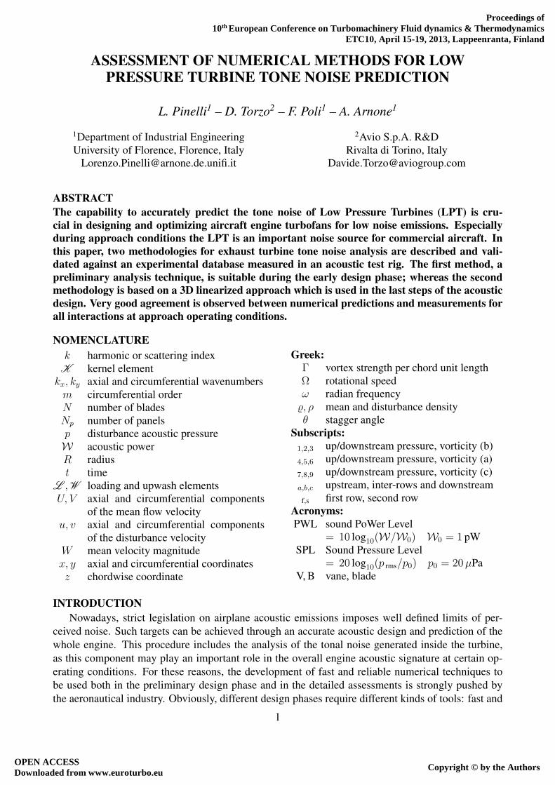
Solving the coupled systemOnce the large matrix describing the generation or propagation problem has been filled in and

the upwash vector has been built the unsteady load can be computed by solving the linear systemTo efficiently do this the optimized LAPACK library (Anderson et al (1999)) routine based on theLU factorization in OpenMP parallelism was chosen Now for acoustic purposes it is necessary toderive the SPL of each acoustic wave generated by the unsteady load of both rows in upstream anddownstream regions This can be accomplished by using the transmission coefficients T and thenequations 3 Finally to obtain the PWL the classical formula of the acoustic intensity projected inaxial direction can be used

~I =

(p

+ ~w middot ~W

)(~w + ρ ~W

)=rArr Ix = ~I middot ~ix =

(p

+ Uu+ V v

)(u+

p

a2U)

(12)

The acoustic powerW is the time average of Ix integrated over the duct cross sectional area A Sincethe concept of duct area is not defined in this 2D analysis it is appropriate to compute the averagepower per unit area as follows

WA

=1

2π

int 2π

0

1

T

int T

0

Ix dt dφ whereφ is the longitudinal angle (13)

Fully 3D linearized methodThe 3D method for acoustic prediction is based on a time-linearized aeroelastic and aeroacoustic

solver named Lars The Lars code is able to deal with incoming perturbations due to unsteady interac-tions with upstreamdownstream rows (tone noise) which are treated with a non-reflecting boundarycondition approach based on radial mode decomposition (Poli et al (2009))

For the numerical evaluation of the tone noise reaching the turbine exit both generation andpropagation phenomena have to be properly simulated and for this reason the single blade aeroa-coustic solver was integrated into a proper propagation procedure Generation of the sound is handledby means of a wave splitting method while the propagation method consists of a sequence of lin-earized aeroacoustic computations which transmit the most relevant waves in the propagation direc-tion Moreover to have a better insight of the physical mechanisms which govern certain behaviorsthe propagation analysis has necessarily to account for the 3D physics of waves in annular ductsHence it is important that the propagation strategy follow the evolution of each acoustic mode fromits source up to the engine exit taking into account the radial shape of the traveling perturbations Theprocedure developed by the authors may be applied to both downstream and upstream running wavesand is suitable for turbine as well as compressorfan applications Further details of this method canbe found in Pinelli et al (2011a)

ACOUSTIC TEST RIGEngine noise measurements usually provide overall qualitative information on propagating turbine

tones and associated noise levels engine acoustic data are representative of the whole propulsion sys-tem and the rear arc spectrum includes several acoustic contributions as well as installation effectsFor this reason the identification of turbine emissions is not straightforward and is mainly based onfrequency and directivity data In this context a cold flow rig becomes a very attractive way to gain adeeper physical understanding and to have a high-quality detailed dataset for a direct and completevalidation of noise generation and in-duct propagation tools Acoustic cold flow measurements pro-vide a relation between acquired acoustic data and the generating turbine The identification of theLPT acoustic emissions is based on the circumferential and radial mode order detection technique

7

Starting from the above considerations an acoustic cold flow rig (Taddei et al (2009)) has been re-cently set up at Avio (see figure 3) The acoustic measurements coming from first test campaignshave already been used for CAA validation (Pinelli et al (2011a)) generally highlighting a goodagreement between numerical prediction and experimental data

Figure 3 Cold flow rig (left) 1st vane geometry with instrumented blades removed (right) andkulite rake (box)

The Avio annular rig has a modular design which allows easy replacement of rows variation ofrow axial spacing and addition of rows (inlet or outlet guide vanes single-stage to two-stage setups)In designing the model turbine engine-to-rig similitude criteria have been followed (such as Machnumber similarity) blade geometries loadings and flow deflections have been selected according tostate-of-the-art design of a commercial aeroengine LPT while the airfoil count provides aeroacousticsimilitude in terms of reduced frequency The rig operates at ambient exit pressure and the overpres-sure at inlet is provided by a compressor A flat endwall geometry was chosen which is representativeof the turbine rear stages and allows for easy rig assembly

Concerning measurement capabilities both aerodynamic and acoustic instrumentation have beeninstalled The aerodynamic instrumentation is aimed at characterizing the turbine operating condi-tions and resolving the mean flow field at turbine inlet and outlet As far as the noise measurementsare concerned a rotating duct at turbine exit has been introduced to permit the detailed mapping of thegenerated acoustic field and its propagation pattern by means of two kulite rakes Other measurementdevices are available in the cold flow ie axial arrays of flush-mounted microphones Currently themicrophones are used for confirmation of the kulite measurements in the mid-low frequency rangeThe azimuthal positioning system allows for collecting of a sufficient number of acoustic pressuredata along the circumferential direction to detect all relevant cut-on modes at the various flow condi-tions (namely approach and cutback conditions plus other additional operating points) High speedacquisition hardware is used allowing the simultaneous acquisition of all unsteady pressure signalsAdditionally a one pulse per revolution is recorded to allow synchronous re-sampling of pressuresignals aimed at increasing the signal-to-noise ratio and avoiding detrimental effects due to rotorspeed variations (hence improving the global accuracy of the analysis) Finally based on the acousticfield mapping complemented by flow field description modal decomposition techniques (extendedto account for swirling flow) have been applied and propagating modes detected The comparisonsdescribed in the following section refer to an experimental campaign where a two-stage turbine wastested with the addition of a leaned Turbine Rear Frame (TRF)

8

LPT TONE NOISE RESULTSIn the following selected comparisons between experimental and numerical results of the acoustic

test rig at the approach configuration will be presented and discussed This operating point was chosensince it turns out to be the most critical for LPT tone noise emissions At the time of writing differentoperating conditions and turbine setups are still under investigation

Comparison between experimental and numerical resultsThe measured acoustic spectrum at turbine exhaust for approach conditions has been processed

by RMA (Radial Mode Analysis see Taddei et al (2009)) to show the modal content of the acousticpressure field for each selected frequency The results highlight a pronounced relevance of peakscaused by the rotor-stator interactions especially at the 1st blade passing frequency (BPF) of the firstrotor since the V1-B1 interaction is designed for being cut-on These peaks are connected to thegenerating interactions by means of a circumferential analysis In this way the relevant interactions(reported in figure 4) can be identified and then analyzed numerically

Figure 4 Cold flow rig geometry of the rows

V1minusB1 V2minusB2 B2minusTRF

PW

L t

ota

l [d

B]

10 dB

APPROACHmeasured

computed (Lars 3D)

computed (TNT 2D)

Figure 5 Total PWL at the turbine exhaust

The three interactions being analyzed have different behaviors inside the turbine (cut-oncut-off)yet they all produce a lot of cut-on waves at the TRF exit A comparison of total PWL emissions ofsuch interactions are shown in figure 5 As can be seen the agreement is very good and the differencesbetween measurements and 3D calculations are within 15 dB The mesh dimensions used for the 3D

minus15 minus14 minus13 minus12 minus11 minus10 minus9 minus8 minus7 minus6 minus5 minus4 minus3 minus2 minus1 0 1 2 3 4 5 6 7 8 9 10 11 12 13 14 15

PW

L [

dB

]

circumferential order (m)

10 dB

measured

computed (Lars 3D)

Figure 6 Modal decomposition results for the 1st BPF (B1) at the turbine exit

9

calculations are approximately 180times100times80 for each inter-blade vane ensuring at least 30 cells perconvected wavelength and 70 cell per acoustic wavelength However the preliminary design toolresults also agree well with the measurements despite the strong assumption of flat plate geometrieswhich could be a possible source of discrepancy This approach tends to overestimate the emissionsthis may also be due to the fact that the 2D tool computes an average power per unit area which isthen considered constant over the duct area to get the total PWL However this simplified methodis able to reproduce the correct relative relevance of the studied emissions confirming its usefulnessin the early steps of machine design For each BPF the total power at TRF exit can be split up intomodal orders to highlight the effect of TRF scattering Figure 6 shows the modal decomposition forthe 1st BPF of the first rotor The arrows indicate the components related to the V1-B1 interactionin comparison to the 3D results after the scattering effect of the TRF Measurements and numericalpredictions are in really good agreement Analogous considerations can be made for the modal resultsat the 1st BPF of the second rotor showing the V2-B2 and B2-TRF interactions This mode splitting

minus14 minus5 4 13

PW

L [

dB

]

circumferential order (m)

10 dB

V1minusB1

measured

computed (Lars 3D)

computed (TNT 2D)

minus15 minus6 3 12

PW

L [

dB

]

circumferential order (m)

10 dB

V2minusB2

measured

computed (Lars 3D)

computed (TNT 2D)

Figure 7 Comparison of modal components V1-B1 (left) and V2-B2 (right)

was also computed by the preliminary tool and the results for V1-B1 and V2-B2 interactions aresummarized in figure 7 As expected the 3D method which is able to account for the radial shape ofacoustic perturbations gives a better agreement with measurements in terms of PWL splitting withrespect to the preliminary analysis tool

CONCLUSIONSTwo prediction methods for LPT tone noise emissions have been presented an analytic tool aimed

at the preliminary evaluation of the LPT acoustic design and a 3D CAA linearized approach suitablefor the detailed design phase The acoustic predictions provided by both methods have been comparedto the experimental results coming from an acoustic test campaign carried out on a cold flow rig atAvio the highlighted agreement is very good especially for the 3D results This demonstrates theprediction capability of the methods and confirms their usefulness as design tools

ACKNOWLEDGMENTSThe authors would like to acknowledge Avio SpA for the financial support and the permission

to publish Special thanks to Dr Francesco Taddei (Department of Industrial Engineering Universityof Florence) for his useful technical contribution

10

REFERENCESAmiet R (1974) Transmission and reflection of sound by two blade rows Journal of Sound and

Vibration 34 (3)399ndash412Anderson E Bai Z Bischof C Blackford S Demmel J Dongarra J Croz J D Greenbaum

A Hammarling S McKenney A and Sorensen D (1999) LAPACK Usersrsquo Guide Society forIndustrial and Applied Mathematics Philadelphia PA third edition

Arnone A Poli F and Schipani C (2003) A method to assess flutter stability of complex modesIn 10th International Symposium on Unsteady Aerodynamics Aeroacoustics and Aeroelasticity ofTurbomachines

Boncinelli P Marconcini M Poli F Arnone A and Schipani C (2006) Time-linearized quasi-3D tone noise computations in cascade flows In IGTI ASME Turbo Expo ASME paper GT2006-90080

Campobasso M and Giles M (2003) Effects of flow instabilities on the linear analysis of turboma-chinery aeroelasticity Journal of propulsion and power 19(2)250ndash259

Chassaing J-C and Gerolymos G (2000) Compressor flutter analysis using time-nonlinear andtime-linearized 3-D Navier-Stokes methods In 9th International Symposium on Unsteady Aerody-namics Aeroacoustics and Aeroelasticity of Turbomachines

Frey C Ashcroft G Kersken H and Weckmuller C (2012) Advanced numerical methods forthe prediction of tonal noise in turbomachinery part II Time-linearized methods In IGTI ASMETurbo Expo ASME paper GT2012-69418

Hall K and Clark W (1993) Linearized Euler predictions of unsteady aerodynamic loads in cas-cades AIAA Journal 31540ndash550

Hall K Ekici K and Voytovych D (2006) Multistage coupling for unsteady flows in turbo-machinery In Unsteady Aerodynamics Aeroacoustics and aeroelasticity of turbomachines pages217ndash229 Springer Netherlands

Hall K and Lorence C (1993) Calculation of three-dimensional unsteady flows in turbomachineryusing the linearized harmonic Euler equations Transactions of the ASME Journal of turbomachin-ery 115800ndash809

Hanson D (1994) Coupled 2-dimensional cascade theory for noise and unsteady aerodynamicsof blade row interaction in turbofans Volume 1 ndash Theory development and parametric studiesTechnical report NASA Contractor Report 4506

Hanson D (2001) Broadband noise of fans ndash with unsteady coupling theory to account for rotor andstator reflectiontransmission effects Technical report NASA Contractor Report 211136

Heinig K (1983) Sound propagation in multistage axial flow turbomachines AIAA Journal 1598ndash105

Kaji S and Okazaki T (1970) Generation of sound by rotorndashstator interation Journal of Sound andVibration 13(3)281ndash307

Kennepohl F Kahl G and Heinig K (2001) Turbine bladevane interaction noise Calculationwith a 3D time-linearised Euler method In 7th AIAACEAS Aeroacoustic Conference

Koch W (1971) On the transmission of sound waves through a blade row Journal of Sound andVibration 18 (1)111ndash128

Korte D Huttl T Kennepohl F and Heinig K (2005) Numerical simulation of a multistageturbine sound generation and propagation Aerospace science and tecnology 9125ndash134

Pinelli L Poli F Marconcini M Arnone A Spano E and Torzo D (2011a) Validation of a3d linearized method for turbomachinery tone noise analysis In IGTI ASME Turbo Expo ASMEpaper GT2011-45886

11

Pinelli L Poli F Marconcini M Arnone A Spano E Torzo D and Schipani C (2011b) Alinearized method for tone noise generation and propagation analysis in a multistage contra-rotatingturbine In 9th European Conference on Turbomachinery Fluid Dynamics and Thermodynamics

Poli F Arnone A and Schipani C (2009) A 3D linearized method for turbomachinery tone noiseanalysis with 3D non-reflecting boundary conditions In 8th European Conference on Turboma-chinery Fluid Dynamics and Thermodynamics

Poli F Gambini E Arnone A and Schipani C (2006) A 3D time-linearized method for tur-bomachinery blade flutter analysis In 11th International Symposium on Unsteady AerodynamicsAeroacoustics and Aeroelasticity of Turbomachines

Posson H Roger M and Moreau S (2010) On a uniformly valid analytical rectilinear cascaderesponse function Journal of Fluid Mechanics 66322ndash52

Smith N (1973) Discrete frequency sound generation in axial flow turbomachines Technical reportReport R amp M no 3709

Taddei F Cinelli C De Lucia M and Schipani C (2009) Experimental investigation of lowpressure turbine noise Radial mode analysis for swirling flows In 12th International Symposiumon Unsteady Aerodynamics Aeroacoustics and Aeroelasticity of Turbomachines

Tyler J and Sofrin T (1962) Axial flow compressor noise studies Trans Society of AutomotiveEngineers 70309ndash332

Ventres C Theobald M and Mark W (1982) Turbofan noise generation vol I Analysis Tech-nical report NASA Contractor Report 167952

12

robust techniques for the preliminary choices accurate and reliable methods for the advanced designverification

Over the past four decades countless methods have been developed to predict the acoustic emis-sion at blade passing frequencies The first major contribution to the aeroacoustics of turbomachinerycan be attributed to Tyler and Sofrin (1962) who determined the link between blade count and ductmodes and their propagation behavior (cut-on or cut-off) Early methods to compute the strength ofthese spinning modes were based on analytic models derived from flat plate theory (Amiet (1974)Koch (1971)) where the sound emissions mainly depend on the difference between the wave angleand the stagger angle of the flat plate Then Ventres et al (1982) proposed a method which linked a2D flat plate theory for the unsteady aerodynamics to the acoustic modes of the actual 3D annular ductby means of strip analysis Other methods can be found in the literature Kaji and Okazaki (1970)developed a coupled statorrotor theory which however limited the analysis to a single frequency anddid not include the swirl effect On the contrary the methodology provided by Heinig (1983) maybe applied to turbomachines with non-uniform swirling flows A more accurate 3D analytical modelis presented by Posson et al (2010) Since the 1990s thanks to the growth in computer technologyldquotime-linearizedrdquo methods have been developed capable of dealing with real blade geometries andnon-uniform mean flows (Hall and Clark (1993) Hall and Lorence (1993) Chassaing and Gerolymos(2000) Campobasso and Giles (2003) Kennepohl et al (2001)) Such methods were first employedto evaluate the acoustic response of a single blade row but can also be efficiently used to predict thetone noise emission at the turbine exit by integrating the time-linearized code in a proper propagationprocedure (Korte et al (2005) Pinelli et al (2011a) Frey et al (2012))

In this paper two different approaches for tonal noise evaluation of a low pressure turbine willbe presented The first one a preliminary analysis technique is suitable for the early design phasewhereas the other one a 3D linearized method can be used in the last steps of the acoustic design

The preliminary acoustic tool is able to quickly estimate the tone noise emissions of a multistageLPT The method is based on simple mean line aerodynamic data and takes into account both acousticgeneration and propagation phenomena For this reason it can be seen as an extension of Hansonrsquoscoupled 2D cascade theory (Hanson (1994)) it extends Hansonrsquos theory for a single fan stage (tworows) to a multi-stage system (turbine) Adjacent blade rows are modeled as 2D flat plate cascadesand are included in a fully coupled unsteady analysis which satisfies the flow tangency boundarycondition on both rows simultaneously for several harmonics In this way noise generation scatteringand reflections are accounted for by solving a large linear system Further the swirling flow betweenadjacent rows is considered by means of actuator disks Following this approach the method de-scribes the evolution of the turbine-generated acoustic modes along the machine and provides foreach of them SPL and PWL values at the exhaust section

On the other hand the linearized method already described by the authors in previous works(Arnone et al (2003) Poli et al (2006) Boncinelli et al (2006) Poli et al (2009)) is based on afully three-dimensional aeroacoustic solver integrated in a proper propagation strategy (Pinelli et al(2011ba)) and can be fruitfully used during the detailed acoustic design

A wide validation of both tools is reported based on the experimental database measured in anacoustic test rig representative of the last stages of a low-pressure turbine All these activities arecarried out in the context of a research project on turbomachinery Computational Aeroelasticity (CA)and Computational Aeroacoustics (CAA) at the Department of Industrial Engineering (University ofFlorence) in collaboration with Avio SpA

THEORY OF THE NOISE PREDICTION METHODSThis section describes the theoretical basis of the two numerical methods which will be used to

predict acoustic emissions of a LPT for aeronautical applications Special emphasis will be put on the

2

preliminary analysis tool based on a semi-analytical method the 3D linearized method will be onlybriefly presented as it has already been described by the authors in (Pinelli et al (2011a))

Preliminary analysis toolThe preliminary analysis tool (named TNT Tone Noise Tool) is an extension of Hansonrsquos coupled

cascade theory from fan to LPT applications although it is acknowledged that the flat plate assump-tion is stronger for a turbine environment than for a fanOGV interaction Moreover the methodextension allows the analysis not only of the tone noise generation as did the original theory butalso of the acoustic propagation through successive rows up to turbine exhaust The tool which wasdeveloped computes the interaction between two adjacent blade rows (see right side of figure 1) andestimates either the effect of the wake from the upstream blade rows impinging on the successiveblade row (generation module) or the effect of an acoustic wave imposed in the gap between rows(propagation module) These interactions produce unsteady loading on both rows and thereby gener-ate outgoing acoustic waves The model takes into account reflectiontransmission characteristics andthe swirling flow between the two rows by means of actuator disk theory Unlike simpler methods inwhich there is a one-to-one relationship between wake harmonics and noise harmonics the presentedmethod simultaneously couples the effects of multiple harmonics in a large linear system In thisway noise generation scattering and reflections effects can be included in the model The solutionof the linear system is the unsteady loading distribution on both rows for each harmonic caused byincoming perturbations Once the unsteady loading is computed it is simple to derive the resultingoutput waves in terms of SPL and PWL

Basic theoryThe basis of Hansonrsquos coupled 2D theory is Smithrsquos theory (Smith (1973)) Smith derived a theo-

retical approach which relates the unsteady loading of a single cascade of flat plates with a specifiedvelocity disturbance entering the system This approach is based on an integral equation for the up-wash velocity (disturbance velocity component normal to the blade chord see left side of figure 1)on the cascade caused by the unknown load distribution The resulting equations can be solved for

0 xs xe

sf

ss

cf cs

x

y

θs

ΩfR ΩsR

1st row 2nd row

uimp

vimp

wake(generationmodule)

acoustic wave

(propagationmodule)

zs

zf

Smiths theory extended Hansons theory

0

y

VW

U

cu

v

unsteadyvelocity

v

u

vcosθ-usinθw

upwashvelocity

meanvelocity

θ x

zs

Figure 1 Geometry of Smithrsquos theory (left) and geometry of coupled cascade (right)

the loads and hence the outgoing acoustic waves can be evaluated As usual in acoustics Smith startswith the linearized differential equations for continuity and momentum and assumes the following

3

form for velocity and pressure perturbations (complex quantities are marked with the oversign ˜)uvp

= lte

uvp

e (kxx + kyy + ωt)

where ky =m

R(1)

This analysis leads to two families of solutions of the continuity and momentum equations the firstfamily includes the pressure waves which propagate updownstream (with or without attenuation)at the speed of sound a while the second one contains the vorticity waves which are convecteddownstream by the mean flow The respective axial wave numbers are given by

kx 12 =U(ω + V ky)plusmn a

radic(ω + V ky)2 minus (a2 minus U2)k2y

a2 minus U2kx 3 = minus(ω + V ky)

U(2)

Moreover the relations between velocity and pressure complex mode amplitudes are

u12 = kx 12v12ky

p12 = minus(ω + Ukx 12 + V ky)v12ky

and u3 = minuskyv3kx 3

(3)

Smith then deduces equation 4 which describes the total circumferential perturbation velocity relatedto each wave type

v(total)123 =

int c

0

lte

infinsum

k=minusinfin

vprime123 e(kx 123x + kyy + ωt) eminus(kx 123 cos θ + ky sin θ)z

Γ(z)

sdz (4)

Upstream of the cascade there will be only the v(total)1 component which corresponds to the circumfer-

ential velocity perturbation due to all upstream running pressure waves In the same way anywheredownstream of the row v(total)

2 (sum of downstream running pressure waves) and v(total)3 (sum of vortic-

ity waves) will be present Expressions for vprime1 vprime2 and vprime3 are directly derived from Smithrsquos theory (seeSmith (1973)) and respectively represent the influence of a unit loading element on the updownstreamrunning pressure and vorticity waves Then the load distribution over the blade chord is discretizedinto Np identical panels and the integral is converted to a sum according to

1

c

int zj+∆z2

zjminus∆z2

Γ(z)

Wdz =rArr L (j) where ∆z =

c

Np

(5)

Following Hansonrsquos approach equation 4 can thus be generalized for each row with multiple harmon-ics for any wave type

v(total) =W

sc

+infinsumk fs=minusinfin

Npsumi=1

lte

+infinsum

k sf=minusinfin

vprime e(kxx+ kyy+ωt) eminus(kx cos θ+ ky sin θ)zi

timesL (k fs i) (6)

Wave systemThe next step is to derive the form of all the waves which can result from a generic interaction

between adjacent rows for both generation and propagation cases When dealing with a wave genera-tion phenomenon the classical Tyler and Sofrin spinning modes are generated Such modes form thewave system for the generation module and are described in the fixed reference frame in the left sideof equations 7

m = ksNs minus kfNf

ω = kfNfΩf minus ksNsΩs︸ ︷︷ ︸(generation module)

m = m0 + kfNf + ksNs

ω = ω0 minus kfNfΩf minus ksNsΩs︸ ︷︷ ︸(propagation module)

(7)

4

The present extension of Hansonrsquos theory also allows the propagation of a single mode through suc-cessive rows (one at a time together with the previously analyzed row) This means that the wavesystem describing the propagation problem is different and has to be composed of the imposed wave(with m0 and ω0) together with all the scattering modes due to the two blade rows The wave sys-tem for the propagation module is depicted by the right side of equations 7 The same conclusionwas drawn by Hall et al (2006) in their work on flutter in a multistage environment Furthermoreif the imposed wave (with m0 and ω0) is a vector of turbulence modes right side of equations 7 alsodescribe the set of permitted broadband modes (see Hanson (2001))

Reflection and transmission coefficientsSwirling flow between rows must be considered in order to have a better representation of the

mean flow properties As explained in Hanson (1994) actuator disks can be used to turn the meanflow at the 1st row leading edge and at the 2nd row trailing edge (see figure 2) As the mean flowchanges across the inlet and exit interfaces the unsteady quantities vary as well This can be handledby employing reflection R and transmission T coefficients for all the waves Such coefficients aredirectly derived from the linearized continuity of mass and momentum

1st rowinlet disk

2nd rowexit disk

ρaaaMxa

ρcacMxc

ρbab

Mxb

Ms

v1v2

v3v4v1

v3

v8

v9

v1

v2

v8

v9

T1↦4 R1↦2

R1↦3

R2↦1T2↦8

T2↦9

R3↦1T3↦8

T3↦9

region b(inter-row)

region c(downstream)

region a(upstream)

0 xex

0 xex

1st rowleading edge

2nd rowtrailing edge

(RW1)f

(RW2)f

(RW3)f

(RW1)s

(RW2)s

(RW3)s

Ls

(DW1)s (DW2)s

(DW3)s

Lf

(DW1)f (DW2)f

(DW3)f

Rx↦yreflection coefficient

(from the incident wave x to the

reflected wave y)

Tx↦ytransmission coefficient

(from the wave x to the transmitted

wave y)

RW reflected wave

DW direct wave

Figure 2 Coupled theory reflectiontransmission coefficients (left) waves system (right)

Coupled 2D theoryIn order to couple the problem it is sufficient to construct the wave field between the 1st row

leading edge and the 2nd row trailing edge by means of direct waves coming from each loading element(via Smithrsquos formulae) plus the waves reflected from the inlet and exit interfaces (see figure 2) For aloading element of the 1st row for instance the direct waves (DW123)f from each panel are obtainedby Smithrsquos theory while the reflected waves (RW123)f can be built as follows

(RW1)f = [(DW2)f + (RW2)f]R2rarr1 + [(DW3)f + (RW3)f]R3rarr1

(RW2)f = [(DW1)f + (RW1)f]R1rarr2

(RW3)f = [(DW1)f + (RW1)f]R1rarr3

(8)

5

and similar equations hold for the 2nd row Such coupling equations are written in terms of transversevelocity v123 components Now the axial velocity u123 can be obtained by using equation 3 so thatit is straightforward to derive the upwash velocity (see Hanson (1994)) Together all the couplingequations (such as equations 6 and 8) written in terms of upwash velocity define four sub-matricesof influence and sub-matrices can be assembled into a large matrix representing the entire coupledsystem[

Kfrarrf Ksrarrf

Kfrarrs Ksrarrs

]times[Lf

Ls

]=

[Wf

Ws

](9)

When dealing with the propagation module of the acoustic tool the deeper structure of the coupledlinear system for the special case of minus1 lt kfs lt +1 becomes as shown in equation 10Inside this large system each sub-matrix includes the kernel quantity for each element discretizing thetwo rows It is worth noting how the system explicitly shows the modal and frequency scattering andhow it allows the inclusion of multiple reflections between the rows

Kfrarrfkf = minus1ks = minus1

0

0

Ksrarrfkf = minus1ks = minus1

Ksrarrfkf = 0ks = minus1

Ksrarrfkf = +1ks = minus1

0

Kfrarrfkf = 0ks = 0

0

Ksrarrfkf = minus1ks = 0

Ksrarrfkf = 0ks = 0

Ksrarrfkf = +1ks = 0

0

0

Kfrarrfkf = +1ks = +1

Ksrarrfkf = minus1ks = +1

Ksrarrfkf = 0ks = +1

Ksrarrfkf = +1ks = +1

Kfrarrskf = minus1ks = minus1

Kfrarrskf = 0ks = minus1

Kfrarrskf = +1ks = minus1

Ksrarrskf = minus1ks = minus1

0

0

Kfrarrskf = minus1ks = 0

Kfrarrskf = 0ks = 0

Kfrarrskf = +1ks = 0

0

Ksrarrskf = 0ks = 0

0

Kfrarrskf = minus1ks = +1

Kfrarrskf = 0ks = +1

Kfrarrskf = +1ks = +1

0

0

Ksrarrskf = +1ks = +1

times

Lfkf = minus1

Lfkf = 0

Lfkf = +1

Lsks = minus1

Lsks = 0

Lsks = +1

=

Wfkf = minus1

Wfkf = 0

Wfkf = +1

Wsks = minus1

Wsks = 0

Wsks = +1

(10)

The last point to address is the determination of the upwash array W this can be done by imposingthe no-through-flow boundary condition on both rows Different conditions must be applied to thetwo rows At the 1st row the sum of upwash caused by the row itself and 2nd row is always zero exceptfor the case of upstream pressure propagation (propagation module) where W is the opposite of theupwash due to the imposed pressure wave impinging on the 1st row On the other hand the upwashon the 2nd row is zero only for upstream pressure propagation while in any other case it is causedeither by viscous wake (generation module) or by downstream running pressure wave (propagationmodule)[

Wf

Ws

]=

[Wfrarrf + Wsrarrf

Wfrarrs + Wsrarrs

]=

[0

minusWwake

]︸ ︷︷ ︸

(generation module)

or[minusWup

0

]or[

0minusWdown

]︸ ︷︷ ︸

(propagation module)

(11)

The generation module of the tool requires knowing the wake defect generated by the 1st row in orderto obtain Wwake For this purpose a viscous wake correlation is used In a different way the upwashWup or Wdown for the propagation module is basically composed of the normal components of u vassociated with the updownstream running pressure wave to be propagated Obviously u v comefrom a previous generation or propagation analysis

6

Solving the coupled systemOnce the large matrix describing the generation or propagation problem has been filled in and

the upwash vector has been built the unsteady load can be computed by solving the linear systemTo efficiently do this the optimized LAPACK library (Anderson et al (1999)) routine based on theLU factorization in OpenMP parallelism was chosen Now for acoustic purposes it is necessary toderive the SPL of each acoustic wave generated by the unsteady load of both rows in upstream anddownstream regions This can be accomplished by using the transmission coefficients T and thenequations 3 Finally to obtain the PWL the classical formula of the acoustic intensity projected inaxial direction can be used

~I =

(p

+ ~w middot ~W

)(~w + ρ ~W

)=rArr Ix = ~I middot ~ix =

(p

+ Uu+ V v

)(u+

p

a2U)

(12)

The acoustic powerW is the time average of Ix integrated over the duct cross sectional area A Sincethe concept of duct area is not defined in this 2D analysis it is appropriate to compute the averagepower per unit area as follows

WA

=1

2π

int 2π

0

1

T

int T

0

Ix dt dφ whereφ is the longitudinal angle (13)

Fully 3D linearized methodThe 3D method for acoustic prediction is based on a time-linearized aeroelastic and aeroacoustic

solver named Lars The Lars code is able to deal with incoming perturbations due to unsteady interac-tions with upstreamdownstream rows (tone noise) which are treated with a non-reflecting boundarycondition approach based on radial mode decomposition (Poli et al (2009))

For the numerical evaluation of the tone noise reaching the turbine exit both generation andpropagation phenomena have to be properly simulated and for this reason the single blade aeroa-coustic solver was integrated into a proper propagation procedure Generation of the sound is handledby means of a wave splitting method while the propagation method consists of a sequence of lin-earized aeroacoustic computations which transmit the most relevant waves in the propagation direc-tion Moreover to have a better insight of the physical mechanisms which govern certain behaviorsthe propagation analysis has necessarily to account for the 3D physics of waves in annular ductsHence it is important that the propagation strategy follow the evolution of each acoustic mode fromits source up to the engine exit taking into account the radial shape of the traveling perturbations Theprocedure developed by the authors may be applied to both downstream and upstream running wavesand is suitable for turbine as well as compressorfan applications Further details of this method canbe found in Pinelli et al (2011a)

ACOUSTIC TEST RIGEngine noise measurements usually provide overall qualitative information on propagating turbine

tones and associated noise levels engine acoustic data are representative of the whole propulsion sys-tem and the rear arc spectrum includes several acoustic contributions as well as installation effectsFor this reason the identification of turbine emissions is not straightforward and is mainly based onfrequency and directivity data In this context a cold flow rig becomes a very attractive way to gain adeeper physical understanding and to have a high-quality detailed dataset for a direct and completevalidation of noise generation and in-duct propagation tools Acoustic cold flow measurements pro-vide a relation between acquired acoustic data and the generating turbine The identification of theLPT acoustic emissions is based on the circumferential and radial mode order detection technique

7

Starting from the above considerations an acoustic cold flow rig (Taddei et al (2009)) has been re-cently set up at Avio (see figure 3) The acoustic measurements coming from first test campaignshave already been used for CAA validation (Pinelli et al (2011a)) generally highlighting a goodagreement between numerical prediction and experimental data

Figure 3 Cold flow rig (left) 1st vane geometry with instrumented blades removed (right) andkulite rake (box)

The Avio annular rig has a modular design which allows easy replacement of rows variation ofrow axial spacing and addition of rows (inlet or outlet guide vanes single-stage to two-stage setups)In designing the model turbine engine-to-rig similitude criteria have been followed (such as Machnumber similarity) blade geometries loadings and flow deflections have been selected according tostate-of-the-art design of a commercial aeroengine LPT while the airfoil count provides aeroacousticsimilitude in terms of reduced frequency The rig operates at ambient exit pressure and the overpres-sure at inlet is provided by a compressor A flat endwall geometry was chosen which is representativeof the turbine rear stages and allows for easy rig assembly

Concerning measurement capabilities both aerodynamic and acoustic instrumentation have beeninstalled The aerodynamic instrumentation is aimed at characterizing the turbine operating condi-tions and resolving the mean flow field at turbine inlet and outlet As far as the noise measurementsare concerned a rotating duct at turbine exit has been introduced to permit the detailed mapping of thegenerated acoustic field and its propagation pattern by means of two kulite rakes Other measurementdevices are available in the cold flow ie axial arrays of flush-mounted microphones Currently themicrophones are used for confirmation of the kulite measurements in the mid-low frequency rangeThe azimuthal positioning system allows for collecting of a sufficient number of acoustic pressuredata along the circumferential direction to detect all relevant cut-on modes at the various flow condi-tions (namely approach and cutback conditions plus other additional operating points) High speedacquisition hardware is used allowing the simultaneous acquisition of all unsteady pressure signalsAdditionally a one pulse per revolution is recorded to allow synchronous re-sampling of pressuresignals aimed at increasing the signal-to-noise ratio and avoiding detrimental effects due to rotorspeed variations (hence improving the global accuracy of the analysis) Finally based on the acousticfield mapping complemented by flow field description modal decomposition techniques (extendedto account for swirling flow) have been applied and propagating modes detected The comparisonsdescribed in the following section refer to an experimental campaign where a two-stage turbine wastested with the addition of a leaned Turbine Rear Frame (TRF)

8

LPT TONE NOISE RESULTSIn the following selected comparisons between experimental and numerical results of the acoustic

test rig at the approach configuration will be presented and discussed This operating point was chosensince it turns out to be the most critical for LPT tone noise emissions At the time of writing differentoperating conditions and turbine setups are still under investigation

Comparison between experimental and numerical resultsThe measured acoustic spectrum at turbine exhaust for approach conditions has been processed

by RMA (Radial Mode Analysis see Taddei et al (2009)) to show the modal content of the acousticpressure field for each selected frequency The results highlight a pronounced relevance of peakscaused by the rotor-stator interactions especially at the 1st blade passing frequency (BPF) of the firstrotor since the V1-B1 interaction is designed for being cut-on These peaks are connected to thegenerating interactions by means of a circumferential analysis In this way the relevant interactions(reported in figure 4) can be identified and then analyzed numerically

Figure 4 Cold flow rig geometry of the rows

V1minusB1 V2minusB2 B2minusTRF

PW

L t

ota

l [d

B]

10 dB

APPROACHmeasured

computed (Lars 3D)

computed (TNT 2D)

Figure 5 Total PWL at the turbine exhaust

The three interactions being analyzed have different behaviors inside the turbine (cut-oncut-off)yet they all produce a lot of cut-on waves at the TRF exit A comparison of total PWL emissions ofsuch interactions are shown in figure 5 As can be seen the agreement is very good and the differencesbetween measurements and 3D calculations are within 15 dB The mesh dimensions used for the 3D

minus15 minus14 minus13 minus12 minus11 minus10 minus9 minus8 minus7 minus6 minus5 minus4 minus3 minus2 minus1 0 1 2 3 4 5 6 7 8 9 10 11 12 13 14 15

PW

L [

dB

]

circumferential order (m)

10 dB

measured

computed (Lars 3D)

Figure 6 Modal decomposition results for the 1st BPF (B1) at the turbine exit

9

calculations are approximately 180times100times80 for each inter-blade vane ensuring at least 30 cells perconvected wavelength and 70 cell per acoustic wavelength However the preliminary design toolresults also agree well with the measurements despite the strong assumption of flat plate geometrieswhich could be a possible source of discrepancy This approach tends to overestimate the emissionsthis may also be due to the fact that the 2D tool computes an average power per unit area which isthen considered constant over the duct area to get the total PWL However this simplified methodis able to reproduce the correct relative relevance of the studied emissions confirming its usefulnessin the early steps of machine design For each BPF the total power at TRF exit can be split up intomodal orders to highlight the effect of TRF scattering Figure 6 shows the modal decomposition forthe 1st BPF of the first rotor The arrows indicate the components related to the V1-B1 interactionin comparison to the 3D results after the scattering effect of the TRF Measurements and numericalpredictions are in really good agreement Analogous considerations can be made for the modal resultsat the 1st BPF of the second rotor showing the V2-B2 and B2-TRF interactions This mode splitting

minus14 minus5 4 13

PW

L [

dB

]

circumferential order (m)

10 dB

V1minusB1

measured

computed (Lars 3D)

computed (TNT 2D)

minus15 minus6 3 12

PW

L [

dB

]

circumferential order (m)

10 dB

V2minusB2

measured

computed (Lars 3D)

computed (TNT 2D)

Figure 7 Comparison of modal components V1-B1 (left) and V2-B2 (right)

was also computed by the preliminary tool and the results for V1-B1 and V2-B2 interactions aresummarized in figure 7 As expected the 3D method which is able to account for the radial shape ofacoustic perturbations gives a better agreement with measurements in terms of PWL splitting withrespect to the preliminary analysis tool

CONCLUSIONSTwo prediction methods for LPT tone noise emissions have been presented an analytic tool aimed

at the preliminary evaluation of the LPT acoustic design and a 3D CAA linearized approach suitablefor the detailed design phase The acoustic predictions provided by both methods have been comparedto the experimental results coming from an acoustic test campaign carried out on a cold flow rig atAvio the highlighted agreement is very good especially for the 3D results This demonstrates theprediction capability of the methods and confirms their usefulness as design tools

ACKNOWLEDGMENTSThe authors would like to acknowledge Avio SpA for the financial support and the permission

to publish Special thanks to Dr Francesco Taddei (Department of Industrial Engineering Universityof Florence) for his useful technical contribution

10

REFERENCESAmiet R (1974) Transmission and reflection of sound by two blade rows Journal of Sound and

Vibration 34 (3)399ndash412Anderson E Bai Z Bischof C Blackford S Demmel J Dongarra J Croz J D Greenbaum

A Hammarling S McKenney A and Sorensen D (1999) LAPACK Usersrsquo Guide Society forIndustrial and Applied Mathematics Philadelphia PA third edition

Arnone A Poli F and Schipani C (2003) A method to assess flutter stability of complex modesIn 10th International Symposium on Unsteady Aerodynamics Aeroacoustics and Aeroelasticity ofTurbomachines

Boncinelli P Marconcini M Poli F Arnone A and Schipani C (2006) Time-linearized quasi-3D tone noise computations in cascade flows In IGTI ASME Turbo Expo ASME paper GT2006-90080

Campobasso M and Giles M (2003) Effects of flow instabilities on the linear analysis of turboma-chinery aeroelasticity Journal of propulsion and power 19(2)250ndash259

Chassaing J-C and Gerolymos G (2000) Compressor flutter analysis using time-nonlinear andtime-linearized 3-D Navier-Stokes methods In 9th International Symposium on Unsteady Aerody-namics Aeroacoustics and Aeroelasticity of Turbomachines

Frey C Ashcroft G Kersken H and Weckmuller C (2012) Advanced numerical methods forthe prediction of tonal noise in turbomachinery part II Time-linearized methods In IGTI ASMETurbo Expo ASME paper GT2012-69418

Hall K and Clark W (1993) Linearized Euler predictions of unsteady aerodynamic loads in cas-cades AIAA Journal 31540ndash550

Hall K Ekici K and Voytovych D (2006) Multistage coupling for unsteady flows in turbo-machinery In Unsteady Aerodynamics Aeroacoustics and aeroelasticity of turbomachines pages217ndash229 Springer Netherlands

Hall K and Lorence C (1993) Calculation of three-dimensional unsteady flows in turbomachineryusing the linearized harmonic Euler equations Transactions of the ASME Journal of turbomachin-ery 115800ndash809

Hanson D (1994) Coupled 2-dimensional cascade theory for noise and unsteady aerodynamicsof blade row interaction in turbofans Volume 1 ndash Theory development and parametric studiesTechnical report NASA Contractor Report 4506

Hanson D (2001) Broadband noise of fans ndash with unsteady coupling theory to account for rotor andstator reflectiontransmission effects Technical report NASA Contractor Report 211136

Heinig K (1983) Sound propagation in multistage axial flow turbomachines AIAA Journal 1598ndash105

Kaji S and Okazaki T (1970) Generation of sound by rotorndashstator interation Journal of Sound andVibration 13(3)281ndash307

Kennepohl F Kahl G and Heinig K (2001) Turbine bladevane interaction noise Calculationwith a 3D time-linearised Euler method In 7th AIAACEAS Aeroacoustic Conference

Koch W (1971) On the transmission of sound waves through a blade row Journal of Sound andVibration 18 (1)111ndash128

Korte D Huttl T Kennepohl F and Heinig K (2005) Numerical simulation of a multistageturbine sound generation and propagation Aerospace science and tecnology 9125ndash134

Pinelli L Poli F Marconcini M Arnone A Spano E and Torzo D (2011a) Validation of a3d linearized method for turbomachinery tone noise analysis In IGTI ASME Turbo Expo ASMEpaper GT2011-45886

11

Pinelli L Poli F Marconcini M Arnone A Spano E Torzo D and Schipani C (2011b) Alinearized method for tone noise generation and propagation analysis in a multistage contra-rotatingturbine In 9th European Conference on Turbomachinery Fluid Dynamics and Thermodynamics

Poli F Arnone A and Schipani C (2009) A 3D linearized method for turbomachinery tone noiseanalysis with 3D non-reflecting boundary conditions In 8th European Conference on Turboma-chinery Fluid Dynamics and Thermodynamics

Poli F Gambini E Arnone A and Schipani C (2006) A 3D time-linearized method for tur-bomachinery blade flutter analysis In 11th International Symposium on Unsteady AerodynamicsAeroacoustics and Aeroelasticity of Turbomachines

Posson H Roger M and Moreau S (2010) On a uniformly valid analytical rectilinear cascaderesponse function Journal of Fluid Mechanics 66322ndash52

Smith N (1973) Discrete frequency sound generation in axial flow turbomachines Technical reportReport R amp M no 3709

Taddei F Cinelli C De Lucia M and Schipani C (2009) Experimental investigation of lowpressure turbine noise Radial mode analysis for swirling flows In 12th International Symposiumon Unsteady Aerodynamics Aeroacoustics and Aeroelasticity of Turbomachines

Tyler J and Sofrin T (1962) Axial flow compressor noise studies Trans Society of AutomotiveEngineers 70309ndash332

Ventres C Theobald M and Mark W (1982) Turbofan noise generation vol I Analysis Tech-nical report NASA Contractor Report 167952

12

preliminary analysis tool based on a semi-analytical method the 3D linearized method will be onlybriefly presented as it has already been described by the authors in (Pinelli et al (2011a))

Preliminary analysis toolThe preliminary analysis tool (named TNT Tone Noise Tool) is an extension of Hansonrsquos coupled

cascade theory from fan to LPT applications although it is acknowledged that the flat plate assump-tion is stronger for a turbine environment than for a fanOGV interaction Moreover the methodextension allows the analysis not only of the tone noise generation as did the original theory butalso of the acoustic propagation through successive rows up to turbine exhaust The tool which wasdeveloped computes the interaction between two adjacent blade rows (see right side of figure 1) andestimates either the effect of the wake from the upstream blade rows impinging on the successiveblade row (generation module) or the effect of an acoustic wave imposed in the gap between rows(propagation module) These interactions produce unsteady loading on both rows and thereby gener-ate outgoing acoustic waves The model takes into account reflectiontransmission characteristics andthe swirling flow between the two rows by means of actuator disk theory Unlike simpler methods inwhich there is a one-to-one relationship between wake harmonics and noise harmonics the presentedmethod simultaneously couples the effects of multiple harmonics in a large linear system In thisway noise generation scattering and reflections effects can be included in the model The solutionof the linear system is the unsteady loading distribution on both rows for each harmonic caused byincoming perturbations Once the unsteady loading is computed it is simple to derive the resultingoutput waves in terms of SPL and PWL

Basic theoryThe basis of Hansonrsquos coupled 2D theory is Smithrsquos theory (Smith (1973)) Smith derived a theo-

retical approach which relates the unsteady loading of a single cascade of flat plates with a specifiedvelocity disturbance entering the system This approach is based on an integral equation for the up-wash velocity (disturbance velocity component normal to the blade chord see left side of figure 1)on the cascade caused by the unknown load distribution The resulting equations can be solved for

0 xs xe

sf

ss

cf cs

x

y

θs

ΩfR ΩsR

1st row 2nd row

uimp

vimp

wake(generationmodule)

acoustic wave

(propagationmodule)

zs

zf

Smiths theory extended Hansons theory

0

y

VW

U

cu

v

unsteadyvelocity

v

u

vcosθ-usinθw

upwashvelocity

meanvelocity

θ x

zs

Figure 1 Geometry of Smithrsquos theory (left) and geometry of coupled cascade (right)

the loads and hence the outgoing acoustic waves can be evaluated As usual in acoustics Smith startswith the linearized differential equations for continuity and momentum and assumes the following

3

form for velocity and pressure perturbations (complex quantities are marked with the oversign ˜)uvp

= lte

uvp

e (kxx + kyy + ωt)

where ky =m

R(1)

This analysis leads to two families of solutions of the continuity and momentum equations the firstfamily includes the pressure waves which propagate updownstream (with or without attenuation)at the speed of sound a while the second one contains the vorticity waves which are convecteddownstream by the mean flow The respective axial wave numbers are given by

kx 12 =U(ω + V ky)plusmn a

radic(ω + V ky)2 minus (a2 minus U2)k2y

a2 minus U2kx 3 = minus(ω + V ky)

U(2)

Moreover the relations between velocity and pressure complex mode amplitudes are

u12 = kx 12v12ky

p12 = minus(ω + Ukx 12 + V ky)v12ky

and u3 = minuskyv3kx 3

(3)

Smith then deduces equation 4 which describes the total circumferential perturbation velocity relatedto each wave type

v(total)123 =

int c

0

lte

infinsum

k=minusinfin

vprime123 e(kx 123x + kyy + ωt) eminus(kx 123 cos θ + ky sin θ)z

Γ(z)

sdz (4)

Upstream of the cascade there will be only the v(total)1 component which corresponds to the circumfer-

ential velocity perturbation due to all upstream running pressure waves In the same way anywheredownstream of the row v(total)

2 (sum of downstream running pressure waves) and v(total)3 (sum of vortic-

ity waves) will be present Expressions for vprime1 vprime2 and vprime3 are directly derived from Smithrsquos theory (seeSmith (1973)) and respectively represent the influence of a unit loading element on the updownstreamrunning pressure and vorticity waves Then the load distribution over the blade chord is discretizedinto Np identical panels and the integral is converted to a sum according to

1

c

int zj+∆z2

zjminus∆z2

Γ(z)

Wdz =rArr L (j) where ∆z =

c

Np

(5)

Following Hansonrsquos approach equation 4 can thus be generalized for each row with multiple harmon-ics for any wave type

v(total) =W

sc

+infinsumk fs=minusinfin

Npsumi=1

lte

+infinsum

k sf=minusinfin

vprime e(kxx+ kyy+ωt) eminus(kx cos θ+ ky sin θ)zi

timesL (k fs i) (6)

Wave systemThe next step is to derive the form of all the waves which can result from a generic interaction

between adjacent rows for both generation and propagation cases When dealing with a wave genera-tion phenomenon the classical Tyler and Sofrin spinning modes are generated Such modes form thewave system for the generation module and are described in the fixed reference frame in the left sideof equations 7

m = ksNs minus kfNf

ω = kfNfΩf minus ksNsΩs︸ ︷︷ ︸(generation module)

m = m0 + kfNf + ksNs

ω = ω0 minus kfNfΩf minus ksNsΩs︸ ︷︷ ︸(propagation module)

(7)

4

The present extension of Hansonrsquos theory also allows the propagation of a single mode through suc-cessive rows (one at a time together with the previously analyzed row) This means that the wavesystem describing the propagation problem is different and has to be composed of the imposed wave(with m0 and ω0) together with all the scattering modes due to the two blade rows The wave sys-tem for the propagation module is depicted by the right side of equations 7 The same conclusionwas drawn by Hall et al (2006) in their work on flutter in a multistage environment Furthermoreif the imposed wave (with m0 and ω0) is a vector of turbulence modes right side of equations 7 alsodescribe the set of permitted broadband modes (see Hanson (2001))

Reflection and transmission coefficientsSwirling flow between rows must be considered in order to have a better representation of the

mean flow properties As explained in Hanson (1994) actuator disks can be used to turn the meanflow at the 1st row leading edge and at the 2nd row trailing edge (see figure 2) As the mean flowchanges across the inlet and exit interfaces the unsteady quantities vary as well This can be handledby employing reflection R and transmission T coefficients for all the waves Such coefficients aredirectly derived from the linearized continuity of mass and momentum

1st rowinlet disk

2nd rowexit disk

ρaaaMxa

ρcacMxc

ρbab

Mxb

Ms

v1v2

v3v4v1

v3

v8

v9

v1

v2

v8

v9

T1↦4 R1↦2

R1↦3

R2↦1T2↦8

T2↦9

R3↦1T3↦8

T3↦9

region b(inter-row)

region c(downstream)

region a(upstream)

0 xex

0 xex

1st rowleading edge

2nd rowtrailing edge

(RW1)f

(RW2)f

(RW3)f

(RW1)s

(RW2)s

(RW3)s

Ls

(DW1)s (DW2)s

(DW3)s

Lf

(DW1)f (DW2)f

(DW3)f

Rx↦yreflection coefficient

(from the incident wave x to the

reflected wave y)

Tx↦ytransmission coefficient

(from the wave x to the transmitted

wave y)

RW reflected wave

DW direct wave

Figure 2 Coupled theory reflectiontransmission coefficients (left) waves system (right)

Coupled 2D theoryIn order to couple the problem it is sufficient to construct the wave field between the 1st row

leading edge and the 2nd row trailing edge by means of direct waves coming from each loading element(via Smithrsquos formulae) plus the waves reflected from the inlet and exit interfaces (see figure 2) For aloading element of the 1st row for instance the direct waves (DW123)f from each panel are obtainedby Smithrsquos theory while the reflected waves (RW123)f can be built as follows

(RW1)f = [(DW2)f + (RW2)f]R2rarr1 + [(DW3)f + (RW3)f]R3rarr1

(RW2)f = [(DW1)f + (RW1)f]R1rarr2

(RW3)f = [(DW1)f + (RW1)f]R1rarr3

(8)

5

and similar equations hold for the 2nd row Such coupling equations are written in terms of transversevelocity v123 components Now the axial velocity u123 can be obtained by using equation 3 so thatit is straightforward to derive the upwash velocity (see Hanson (1994)) Together all the couplingequations (such as equations 6 and 8) written in terms of upwash velocity define four sub-matricesof influence and sub-matrices can be assembled into a large matrix representing the entire coupledsystem[

Kfrarrf Ksrarrf

Kfrarrs Ksrarrs

]times[Lf

Ls

]=

[Wf

Ws

](9)

When dealing with the propagation module of the acoustic tool the deeper structure of the coupledlinear system for the special case of minus1 lt kfs lt +1 becomes as shown in equation 10Inside this large system each sub-matrix includes the kernel quantity for each element discretizing thetwo rows It is worth noting how the system explicitly shows the modal and frequency scattering andhow it allows the inclusion of multiple reflections between the rows

Kfrarrfkf = minus1ks = minus1

0

0

Ksrarrfkf = minus1ks = minus1

Ksrarrfkf = 0ks = minus1

Ksrarrfkf = +1ks = minus1

0

Kfrarrfkf = 0ks = 0

0

Ksrarrfkf = minus1ks = 0

Ksrarrfkf = 0ks = 0

Ksrarrfkf = +1ks = 0

0

0

Kfrarrfkf = +1ks = +1

Ksrarrfkf = minus1ks = +1

Ksrarrfkf = 0ks = +1

Ksrarrfkf = +1ks = +1

Kfrarrskf = minus1ks = minus1

Kfrarrskf = 0ks = minus1

Kfrarrskf = +1ks = minus1

Ksrarrskf = minus1ks = minus1

0

0

Kfrarrskf = minus1ks = 0

Kfrarrskf = 0ks = 0

Kfrarrskf = +1ks = 0

0

Ksrarrskf = 0ks = 0

0

Kfrarrskf = minus1ks = +1

Kfrarrskf = 0ks = +1

Kfrarrskf = +1ks = +1

0

0

Ksrarrskf = +1ks = +1

times

Lfkf = minus1

Lfkf = 0

Lfkf = +1

Lsks = minus1

Lsks = 0

Lsks = +1

=

Wfkf = minus1

Wfkf = 0

Wfkf = +1

Wsks = minus1

Wsks = 0

Wsks = +1

(10)

The last point to address is the determination of the upwash array W this can be done by imposingthe no-through-flow boundary condition on both rows Different conditions must be applied to thetwo rows At the 1st row the sum of upwash caused by the row itself and 2nd row is always zero exceptfor the case of upstream pressure propagation (propagation module) where W is the opposite of theupwash due to the imposed pressure wave impinging on the 1st row On the other hand the upwashon the 2nd row is zero only for upstream pressure propagation while in any other case it is causedeither by viscous wake (generation module) or by downstream running pressure wave (propagationmodule)[

Wf

Ws

]=

[Wfrarrf + Wsrarrf

Wfrarrs + Wsrarrs

]=

[0

minusWwake

]︸ ︷︷ ︸

(generation module)

or[minusWup

0

]or[

0minusWdown

]︸ ︷︷ ︸

(propagation module)

(11)

The generation module of the tool requires knowing the wake defect generated by the 1st row in orderto obtain Wwake For this purpose a viscous wake correlation is used In a different way the upwashWup or Wdown for the propagation module is basically composed of the normal components of u vassociated with the updownstream running pressure wave to be propagated Obviously u v comefrom a previous generation or propagation analysis

6

Solving the coupled systemOnce the large matrix describing the generation or propagation problem has been filled in and

the upwash vector has been built the unsteady load can be computed by solving the linear systemTo efficiently do this the optimized LAPACK library (Anderson et al (1999)) routine based on theLU factorization in OpenMP parallelism was chosen Now for acoustic purposes it is necessary toderive the SPL of each acoustic wave generated by the unsteady load of both rows in upstream anddownstream regions This can be accomplished by using the transmission coefficients T and thenequations 3 Finally to obtain the PWL the classical formula of the acoustic intensity projected inaxial direction can be used

~I =

(p

+ ~w middot ~W

)(~w + ρ ~W

)=rArr Ix = ~I middot ~ix =

(p

+ Uu+ V v

)(u+

p

a2U)

(12)

The acoustic powerW is the time average of Ix integrated over the duct cross sectional area A Sincethe concept of duct area is not defined in this 2D analysis it is appropriate to compute the averagepower per unit area as follows

WA

=1

2π

int 2π

0

1

T

int T

0

Ix dt dφ whereφ is the longitudinal angle (13)

Fully 3D linearized methodThe 3D method for acoustic prediction is based on a time-linearized aeroelastic and aeroacoustic

solver named Lars The Lars code is able to deal with incoming perturbations due to unsteady interac-tions with upstreamdownstream rows (tone noise) which are treated with a non-reflecting boundarycondition approach based on radial mode decomposition (Poli et al (2009))

For the numerical evaluation of the tone noise reaching the turbine exit both generation andpropagation phenomena have to be properly simulated and for this reason the single blade aeroa-coustic solver was integrated into a proper propagation procedure Generation of the sound is handledby means of a wave splitting method while the propagation method consists of a sequence of lin-earized aeroacoustic computations which transmit the most relevant waves in the propagation direc-tion Moreover to have a better insight of the physical mechanisms which govern certain behaviorsthe propagation analysis has necessarily to account for the 3D physics of waves in annular ductsHence it is important that the propagation strategy follow the evolution of each acoustic mode fromits source up to the engine exit taking into account the radial shape of the traveling perturbations Theprocedure developed by the authors may be applied to both downstream and upstream running wavesand is suitable for turbine as well as compressorfan applications Further details of this method canbe found in Pinelli et al (2011a)

ACOUSTIC TEST RIGEngine noise measurements usually provide overall qualitative information on propagating turbine

tones and associated noise levels engine acoustic data are representative of the whole propulsion sys-tem and the rear arc spectrum includes several acoustic contributions as well as installation effectsFor this reason the identification of turbine emissions is not straightforward and is mainly based onfrequency and directivity data In this context a cold flow rig becomes a very attractive way to gain adeeper physical understanding and to have a high-quality detailed dataset for a direct and completevalidation of noise generation and in-duct propagation tools Acoustic cold flow measurements pro-vide a relation between acquired acoustic data and the generating turbine The identification of theLPT acoustic emissions is based on the circumferential and radial mode order detection technique

7

Starting from the above considerations an acoustic cold flow rig (Taddei et al (2009)) has been re-cently set up at Avio (see figure 3) The acoustic measurements coming from first test campaignshave already been used for CAA validation (Pinelli et al (2011a)) generally highlighting a goodagreement between numerical prediction and experimental data

Figure 3 Cold flow rig (left) 1st vane geometry with instrumented blades removed (right) andkulite rake (box)

The Avio annular rig has a modular design which allows easy replacement of rows variation ofrow axial spacing and addition of rows (inlet or outlet guide vanes single-stage to two-stage setups)In designing the model turbine engine-to-rig similitude criteria have been followed (such as Machnumber similarity) blade geometries loadings and flow deflections have been selected according tostate-of-the-art design of a commercial aeroengine LPT while the airfoil count provides aeroacousticsimilitude in terms of reduced frequency The rig operates at ambient exit pressure and the overpres-sure at inlet is provided by a compressor A flat endwall geometry was chosen which is representativeof the turbine rear stages and allows for easy rig assembly

Concerning measurement capabilities both aerodynamic and acoustic instrumentation have beeninstalled The aerodynamic instrumentation is aimed at characterizing the turbine operating condi-tions and resolving the mean flow field at turbine inlet and outlet As far as the noise measurementsare concerned a rotating duct at turbine exit has been introduced to permit the detailed mapping of thegenerated acoustic field and its propagation pattern by means of two kulite rakes Other measurementdevices are available in the cold flow ie axial arrays of flush-mounted microphones Currently themicrophones are used for confirmation of the kulite measurements in the mid-low frequency rangeThe azimuthal positioning system allows for collecting of a sufficient number of acoustic pressuredata along the circumferential direction to detect all relevant cut-on modes at the various flow condi-tions (namely approach and cutback conditions plus other additional operating points) High speedacquisition hardware is used allowing the simultaneous acquisition of all unsteady pressure signalsAdditionally a one pulse per revolution is recorded to allow synchronous re-sampling of pressuresignals aimed at increasing the signal-to-noise ratio and avoiding detrimental effects due to rotorspeed variations (hence improving the global accuracy of the analysis) Finally based on the acousticfield mapping complemented by flow field description modal decomposition techniques (extendedto account for swirling flow) have been applied and propagating modes detected The comparisonsdescribed in the following section refer to an experimental campaign where a two-stage turbine wastested with the addition of a leaned Turbine Rear Frame (TRF)

8

LPT TONE NOISE RESULTSIn the following selected comparisons between experimental and numerical results of the acoustic

test rig at the approach configuration will be presented and discussed This operating point was chosensince it turns out to be the most critical for LPT tone noise emissions At the time of writing differentoperating conditions and turbine setups are still under investigation

Comparison between experimental and numerical resultsThe measured acoustic spectrum at turbine exhaust for approach conditions has been processed

by RMA (Radial Mode Analysis see Taddei et al (2009)) to show the modal content of the acousticpressure field for each selected frequency The results highlight a pronounced relevance of peakscaused by the rotor-stator interactions especially at the 1st blade passing frequency (BPF) of the firstrotor since the V1-B1 interaction is designed for being cut-on These peaks are connected to thegenerating interactions by means of a circumferential analysis In this way the relevant interactions(reported in figure 4) can be identified and then analyzed numerically

Figure 4 Cold flow rig geometry of the rows

V1minusB1 V2minusB2 B2minusTRF

PW

L t

ota

l [d

B]

10 dB

APPROACHmeasured

computed (Lars 3D)

computed (TNT 2D)

Figure 5 Total PWL at the turbine exhaust

The three interactions being analyzed have different behaviors inside the turbine (cut-oncut-off)yet they all produce a lot of cut-on waves at the TRF exit A comparison of total PWL emissions ofsuch interactions are shown in figure 5 As can be seen the agreement is very good and the differencesbetween measurements and 3D calculations are within 15 dB The mesh dimensions used for the 3D

minus15 minus14 minus13 minus12 minus11 minus10 minus9 minus8 minus7 minus6 minus5 minus4 minus3 minus2 minus1 0 1 2 3 4 5 6 7 8 9 10 11 12 13 14 15

PW

L [

dB

]

circumferential order (m)

10 dB

measured

computed (Lars 3D)

Figure 6 Modal decomposition results for the 1st BPF (B1) at the turbine exit

9

calculations are approximately 180times100times80 for each inter-blade vane ensuring at least 30 cells perconvected wavelength and 70 cell per acoustic wavelength However the preliminary design toolresults also agree well with the measurements despite the strong assumption of flat plate geometrieswhich could be a possible source of discrepancy This approach tends to overestimate the emissionsthis may also be due to the fact that the 2D tool computes an average power per unit area which isthen considered constant over the duct area to get the total PWL However this simplified methodis able to reproduce the correct relative relevance of the studied emissions confirming its usefulnessin the early steps of machine design For each BPF the total power at TRF exit can be split up intomodal orders to highlight the effect of TRF scattering Figure 6 shows the modal decomposition forthe 1st BPF of the first rotor The arrows indicate the components related to the V1-B1 interactionin comparison to the 3D results after the scattering effect of the TRF Measurements and numericalpredictions are in really good agreement Analogous considerations can be made for the modal resultsat the 1st BPF of the second rotor showing the V2-B2 and B2-TRF interactions This mode splitting

minus14 minus5 4 13

PW

L [

dB

]

circumferential order (m)

10 dB

V1minusB1

measured

computed (Lars 3D)

computed (TNT 2D)

minus15 minus6 3 12

PW

L [

dB

]

circumferential order (m)

10 dB

V2minusB2

measured

computed (Lars 3D)

computed (TNT 2D)

Figure 7 Comparison of modal components V1-B1 (left) and V2-B2 (right)

was also computed by the preliminary tool and the results for V1-B1 and V2-B2 interactions aresummarized in figure 7 As expected the 3D method which is able to account for the radial shape ofacoustic perturbations gives a better agreement with measurements in terms of PWL splitting withrespect to the preliminary analysis tool

CONCLUSIONSTwo prediction methods for LPT tone noise emissions have been presented an analytic tool aimed

at the preliminary evaluation of the LPT acoustic design and a 3D CAA linearized approach suitablefor the detailed design phase The acoustic predictions provided by both methods have been comparedto the experimental results coming from an acoustic test campaign carried out on a cold flow rig atAvio the highlighted agreement is very good especially for the 3D results This demonstrates theprediction capability of the methods and confirms their usefulness as design tools

ACKNOWLEDGMENTSThe authors would like to acknowledge Avio SpA for the financial support and the permission

to publish Special thanks to Dr Francesco Taddei (Department of Industrial Engineering Universityof Florence) for his useful technical contribution

10

REFERENCESAmiet R (1974) Transmission and reflection of sound by two blade rows Journal of Sound and

Vibration 34 (3)399ndash412Anderson E Bai Z Bischof C Blackford S Demmel J Dongarra J Croz J D Greenbaum

A Hammarling S McKenney A and Sorensen D (1999) LAPACK Usersrsquo Guide Society forIndustrial and Applied Mathematics Philadelphia PA third edition

Arnone A Poli F and Schipani C (2003) A method to assess flutter stability of complex modesIn 10th International Symposium on Unsteady Aerodynamics Aeroacoustics and Aeroelasticity ofTurbomachines

Boncinelli P Marconcini M Poli F Arnone A and Schipani C (2006) Time-linearized quasi-3D tone noise computations in cascade flows In IGTI ASME Turbo Expo ASME paper GT2006-90080

Campobasso M and Giles M (2003) Effects of flow instabilities on the linear analysis of turboma-chinery aeroelasticity Journal of propulsion and power 19(2)250ndash259

Chassaing J-C and Gerolymos G (2000) Compressor flutter analysis using time-nonlinear andtime-linearized 3-D Navier-Stokes methods In 9th International Symposium on Unsteady Aerody-namics Aeroacoustics and Aeroelasticity of Turbomachines

Frey C Ashcroft G Kersken H and Weckmuller C (2012) Advanced numerical methods forthe prediction of tonal noise in turbomachinery part II Time-linearized methods In IGTI ASMETurbo Expo ASME paper GT2012-69418

Hall K and Clark W (1993) Linearized Euler predictions of unsteady aerodynamic loads in cas-cades AIAA Journal 31540ndash550

Hall K Ekici K and Voytovych D (2006) Multistage coupling for unsteady flows in turbo-machinery In Unsteady Aerodynamics Aeroacoustics and aeroelasticity of turbomachines pages217ndash229 Springer Netherlands

Hall K and Lorence C (1993) Calculation of three-dimensional unsteady flows in turbomachineryusing the linearized harmonic Euler equations Transactions of the ASME Journal of turbomachin-ery 115800ndash809

Hanson D (1994) Coupled 2-dimensional cascade theory for noise and unsteady aerodynamicsof blade row interaction in turbofans Volume 1 ndash Theory development and parametric studiesTechnical report NASA Contractor Report 4506

Hanson D (2001) Broadband noise of fans ndash with unsteady coupling theory to account for rotor andstator reflectiontransmission effects Technical report NASA Contractor Report 211136

Heinig K (1983) Sound propagation in multistage axial flow turbomachines AIAA Journal 1598ndash105

Kaji S and Okazaki T (1970) Generation of sound by rotorndashstator interation Journal of Sound andVibration 13(3)281ndash307

Kennepohl F Kahl G and Heinig K (2001) Turbine bladevane interaction noise Calculationwith a 3D time-linearised Euler method In 7th AIAACEAS Aeroacoustic Conference

Koch W (1971) On the transmission of sound waves through a blade row Journal of Sound andVibration 18 (1)111ndash128

Korte D Huttl T Kennepohl F and Heinig K (2005) Numerical simulation of a multistageturbine sound generation and propagation Aerospace science and tecnology 9125ndash134

Pinelli L Poli F Marconcini M Arnone A Spano E and Torzo D (2011a) Validation of a3d linearized method for turbomachinery tone noise analysis In IGTI ASME Turbo Expo ASMEpaper GT2011-45886

11

Pinelli L Poli F Marconcini M Arnone A Spano E Torzo D and Schipani C (2011b) Alinearized method for tone noise generation and propagation analysis in a multistage contra-rotatingturbine In 9th European Conference on Turbomachinery Fluid Dynamics and Thermodynamics

Poli F Arnone A and Schipani C (2009) A 3D linearized method for turbomachinery tone noiseanalysis with 3D non-reflecting boundary conditions In 8th European Conference on Turboma-chinery Fluid Dynamics and Thermodynamics

Poli F Gambini E Arnone A and Schipani C (2006) A 3D time-linearized method for tur-bomachinery blade flutter analysis In 11th International Symposium on Unsteady AerodynamicsAeroacoustics and Aeroelasticity of Turbomachines

Posson H Roger M and Moreau S (2010) On a uniformly valid analytical rectilinear cascaderesponse function Journal of Fluid Mechanics 66322ndash52

Smith N (1973) Discrete frequency sound generation in axial flow turbomachines Technical reportReport R amp M no 3709

Taddei F Cinelli C De Lucia M and Schipani C (2009) Experimental investigation of lowpressure turbine noise Radial mode analysis for swirling flows In 12th International Symposiumon Unsteady Aerodynamics Aeroacoustics and Aeroelasticity of Turbomachines

Tyler J and Sofrin T (1962) Axial flow compressor noise studies Trans Society of AutomotiveEngineers 70309ndash332

Ventres C Theobald M and Mark W (1982) Turbofan noise generation vol I Analysis Tech-nical report NASA Contractor Report 167952

12

form for velocity and pressure perturbations (complex quantities are marked with the oversign ˜)uvp

= lte

uvp

e (kxx + kyy + ωt)

where ky =m

R(1)

This analysis leads to two families of solutions of the continuity and momentum equations the firstfamily includes the pressure waves which propagate updownstream (with or without attenuation)at the speed of sound a while the second one contains the vorticity waves which are convecteddownstream by the mean flow The respective axial wave numbers are given by

kx 12 =U(ω + V ky)plusmn a

radic(ω + V ky)2 minus (a2 minus U2)k2y

a2 minus U2kx 3 = minus(ω + V ky)

U(2)

Moreover the relations between velocity and pressure complex mode amplitudes are

u12 = kx 12v12ky

p12 = minus(ω + Ukx 12 + V ky)v12ky

and u3 = minuskyv3kx 3

(3)

Smith then deduces equation 4 which describes the total circumferential perturbation velocity relatedto each wave type

v(total)123 =

int c

0

lte

infinsum

k=minusinfin

vprime123 e(kx 123x + kyy + ωt) eminus(kx 123 cos θ + ky sin θ)z

Γ(z)

sdz (4)

Upstream of the cascade there will be only the v(total)1 component which corresponds to the circumfer-

ential velocity perturbation due to all upstream running pressure waves In the same way anywheredownstream of the row v(total)

2 (sum of downstream running pressure waves) and v(total)3 (sum of vortic-

ity waves) will be present Expressions for vprime1 vprime2 and vprime3 are directly derived from Smithrsquos theory (seeSmith (1973)) and respectively represent the influence of a unit loading element on the updownstreamrunning pressure and vorticity waves Then the load distribution over the blade chord is discretizedinto Np identical panels and the integral is converted to a sum according to

1

c

int zj+∆z2

zjminus∆z2

Γ(z)

Wdz =rArr L (j) where ∆z =

c

Np

(5)

Following Hansonrsquos approach equation 4 can thus be generalized for each row with multiple harmon-ics for any wave type

v(total) =W

sc

+infinsumk fs=minusinfin

Npsumi=1

lte

+infinsum

k sf=minusinfin

vprime e(kxx+ kyy+ωt) eminus(kx cos θ+ ky sin θ)zi

timesL (k fs i) (6)

Wave systemThe next step is to derive the form of all the waves which can result from a generic interaction

between adjacent rows for both generation and propagation cases When dealing with a wave genera-tion phenomenon the classical Tyler and Sofrin spinning modes are generated Such modes form thewave system for the generation module and are described in the fixed reference frame in the left sideof equations 7

m = ksNs minus kfNf

ω = kfNfΩf minus ksNsΩs︸ ︷︷ ︸(generation module)

m = m0 + kfNf + ksNs

ω = ω0 minus kfNfΩf minus ksNsΩs︸ ︷︷ ︸(propagation module)

(7)

4

The present extension of Hansonrsquos theory also allows the propagation of a single mode through suc-cessive rows (one at a time together with the previously analyzed row) This means that the wavesystem describing the propagation problem is different and has to be composed of the imposed wave(with m0 and ω0) together with all the scattering modes due to the two blade rows The wave sys-tem for the propagation module is depicted by the right side of equations 7 The same conclusionwas drawn by Hall et al (2006) in their work on flutter in a multistage environment Furthermoreif the imposed wave (with m0 and ω0) is a vector of turbulence modes right side of equations 7 alsodescribe the set of permitted broadband modes (see Hanson (2001))

Reflection and transmission coefficientsSwirling flow between rows must be considered in order to have a better representation of the

mean flow properties As explained in Hanson (1994) actuator disks can be used to turn the meanflow at the 1st row leading edge and at the 2nd row trailing edge (see figure 2) As the mean flowchanges across the inlet and exit interfaces the unsteady quantities vary as well This can be handledby employing reflection R and transmission T coefficients for all the waves Such coefficients aredirectly derived from the linearized continuity of mass and momentum

1st rowinlet disk

2nd rowexit disk

ρaaaMxa

ρcacMxc

ρbab

Mxb

Ms

v1v2

v3v4v1

v3

v8

v9

v1

v2

v8

v9

T1↦4 R1↦2

R1↦3

R2↦1T2↦8

T2↦9

R3↦1T3↦8

T3↦9

region b(inter-row)

region c(downstream)

region a(upstream)

0 xex

0 xex

1st rowleading edge

2nd rowtrailing edge

(RW1)f

(RW2)f

(RW3)f

(RW1)s

(RW2)s

(RW3)s

Ls

(DW1)s (DW2)s

(DW3)s

Lf

(DW1)f (DW2)f

(DW3)f

Rx↦yreflection coefficient

(from the incident wave x to the

reflected wave y)

Tx↦ytransmission coefficient

(from the wave x to the transmitted

wave y)

RW reflected wave

DW direct wave

Figure 2 Coupled theory reflectiontransmission coefficients (left) waves system (right)

Coupled 2D theoryIn order to couple the problem it is sufficient to construct the wave field between the 1st row

leading edge and the 2nd row trailing edge by means of direct waves coming from each loading element(via Smithrsquos formulae) plus the waves reflected from the inlet and exit interfaces (see figure 2) For aloading element of the 1st row for instance the direct waves (DW123)f from each panel are obtainedby Smithrsquos theory while the reflected waves (RW123)f can be built as follows

(RW1)f = [(DW2)f + (RW2)f]R2rarr1 + [(DW3)f + (RW3)f]R3rarr1

(RW2)f = [(DW1)f + (RW1)f]R1rarr2

(RW3)f = [(DW1)f + (RW1)f]R1rarr3

(8)

5

and similar equations hold for the 2nd row Such coupling equations are written in terms of transversevelocity v123 components Now the axial velocity u123 can be obtained by using equation 3 so thatit is straightforward to derive the upwash velocity (see Hanson (1994)) Together all the couplingequations (such as equations 6 and 8) written in terms of upwash velocity define four sub-matricesof influence and sub-matrices can be assembled into a large matrix representing the entire coupledsystem[

Kfrarrf Ksrarrf

Kfrarrs Ksrarrs

]times[Lf

Ls

]=

[Wf

Ws

](9)

When dealing with the propagation module of the acoustic tool the deeper structure of the coupledlinear system for the special case of minus1 lt kfs lt +1 becomes as shown in equation 10Inside this large system each sub-matrix includes the kernel quantity for each element discretizing thetwo rows It is worth noting how the system explicitly shows the modal and frequency scattering andhow it allows the inclusion of multiple reflections between the rows

Kfrarrfkf = minus1ks = minus1

0

0

Ksrarrfkf = minus1ks = minus1

Ksrarrfkf = 0ks = minus1

Ksrarrfkf = +1ks = minus1

0

Kfrarrfkf = 0ks = 0

0

Ksrarrfkf = minus1ks = 0

Ksrarrfkf = 0ks = 0

Ksrarrfkf = +1ks = 0

0

0

Kfrarrfkf = +1ks = +1

Ksrarrfkf = minus1ks = +1

Ksrarrfkf = 0ks = +1

Ksrarrfkf = +1ks = +1

Kfrarrskf = minus1ks = minus1

Kfrarrskf = 0ks = minus1

Kfrarrskf = +1ks = minus1

Ksrarrskf = minus1ks = minus1

0

0

Kfrarrskf = minus1ks = 0

Kfrarrskf = 0ks = 0

Kfrarrskf = +1ks = 0

0

Ksrarrskf = 0ks = 0

0

Kfrarrskf = minus1ks = +1

Kfrarrskf = 0ks = +1

Kfrarrskf = +1ks = +1

0

0

Ksrarrskf = +1ks = +1

times

Lfkf = minus1

Lfkf = 0

Lfkf = +1

Lsks = minus1

Lsks = 0

Lsks = +1

=

Wfkf = minus1

Wfkf = 0

Wfkf = +1

Wsks = minus1

Wsks = 0

Wsks = +1

(10)

The last point to address is the determination of the upwash array W this can be done by imposingthe no-through-flow boundary condition on both rows Different conditions must be applied to thetwo rows At the 1st row the sum of upwash caused by the row itself and 2nd row is always zero exceptfor the case of upstream pressure propagation (propagation module) where W is the opposite of theupwash due to the imposed pressure wave impinging on the 1st row On the other hand the upwashon the 2nd row is zero only for upstream pressure propagation while in any other case it is causedeither by viscous wake (generation module) or by downstream running pressure wave (propagationmodule)[

Wf

Ws

]=

[Wfrarrf + Wsrarrf

Wfrarrs + Wsrarrs

]=

[0

minusWwake

]︸ ︷︷ ︸

(generation module)

or[minusWup

0

]or[

0minusWdown

]︸ ︷︷ ︸

(propagation module)

(11)

The generation module of the tool requires knowing the wake defect generated by the 1st row in orderto obtain Wwake For this purpose a viscous wake correlation is used In a different way the upwashWup or Wdown for the propagation module is basically composed of the normal components of u vassociated with the updownstream running pressure wave to be propagated Obviously u v comefrom a previous generation or propagation analysis

6

Solving the coupled systemOnce the large matrix describing the generation or propagation problem has been filled in and

the upwash vector has been built the unsteady load can be computed by solving the linear systemTo efficiently do this the optimized LAPACK library (Anderson et al (1999)) routine based on theLU factorization in OpenMP parallelism was chosen Now for acoustic purposes it is necessary toderive the SPL of each acoustic wave generated by the unsteady load of both rows in upstream anddownstream regions This can be accomplished by using the transmission coefficients T and thenequations 3 Finally to obtain the PWL the classical formula of the acoustic intensity projected inaxial direction can be used

~I =

(p

+ ~w middot ~W

)(~w + ρ ~W

)=rArr Ix = ~I middot ~ix =

(p

+ Uu+ V v

)(u+

p

a2U)

(12)

The acoustic powerW is the time average of Ix integrated over the duct cross sectional area A Sincethe concept of duct area is not defined in this 2D analysis it is appropriate to compute the averagepower per unit area as follows

WA

=1

2π

int 2π

0

1

T

int T

0

Ix dt dφ whereφ is the longitudinal angle (13)

Fully 3D linearized methodThe 3D method for acoustic prediction is based on a time-linearized aeroelastic and aeroacoustic

solver named Lars The Lars code is able to deal with incoming perturbations due to unsteady interac-tions with upstreamdownstream rows (tone noise) which are treated with a non-reflecting boundarycondition approach based on radial mode decomposition (Poli et al (2009))

For the numerical evaluation of the tone noise reaching the turbine exit both generation andpropagation phenomena have to be properly simulated and for this reason the single blade aeroa-coustic solver was integrated into a proper propagation procedure Generation of the sound is handledby means of a wave splitting method while the propagation method consists of a sequence of lin-earized aeroacoustic computations which transmit the most relevant waves in the propagation direc-tion Moreover to have a better insight of the physical mechanisms which govern certain behaviorsthe propagation analysis has necessarily to account for the 3D physics of waves in annular ductsHence it is important that the propagation strategy follow the evolution of each acoustic mode fromits source up to the engine exit taking into account the radial shape of the traveling perturbations Theprocedure developed by the authors may be applied to both downstream and upstream running wavesand is suitable for turbine as well as compressorfan applications Further details of this method canbe found in Pinelli et al (2011a)

ACOUSTIC TEST RIGEngine noise measurements usually provide overall qualitative information on propagating turbine

tones and associated noise levels engine acoustic data are representative of the whole propulsion sys-tem and the rear arc spectrum includes several acoustic contributions as well as installation effectsFor this reason the identification of turbine emissions is not straightforward and is mainly based onfrequency and directivity data In this context a cold flow rig becomes a very attractive way to gain adeeper physical understanding and to have a high-quality detailed dataset for a direct and completevalidation of noise generation and in-duct propagation tools Acoustic cold flow measurements pro-vide a relation between acquired acoustic data and the generating turbine The identification of theLPT acoustic emissions is based on the circumferential and radial mode order detection technique

7

Starting from the above considerations an acoustic cold flow rig (Taddei et al (2009)) has been re-cently set up at Avio (see figure 3) The acoustic measurements coming from first test campaignshave already been used for CAA validation (Pinelli et al (2011a)) generally highlighting a goodagreement between numerical prediction and experimental data

Figure 3 Cold flow rig (left) 1st vane geometry with instrumented blades removed (right) andkulite rake (box)

The Avio annular rig has a modular design which allows easy replacement of rows variation ofrow axial spacing and addition of rows (inlet or outlet guide vanes single-stage to two-stage setups)In designing the model turbine engine-to-rig similitude criteria have been followed (such as Machnumber similarity) blade geometries loadings and flow deflections have been selected according tostate-of-the-art design of a commercial aeroengine LPT while the airfoil count provides aeroacousticsimilitude in terms of reduced frequency The rig operates at ambient exit pressure and the overpres-sure at inlet is provided by a compressor A flat endwall geometry was chosen which is representativeof the turbine rear stages and allows for easy rig assembly

Concerning measurement capabilities both aerodynamic and acoustic instrumentation have beeninstalled The aerodynamic instrumentation is aimed at characterizing the turbine operating condi-tions and resolving the mean flow field at turbine inlet and outlet As far as the noise measurementsare concerned a rotating duct at turbine exit has been introduced to permit the detailed mapping of thegenerated acoustic field and its propagation pattern by means of two kulite rakes Other measurementdevices are available in the cold flow ie axial arrays of flush-mounted microphones Currently themicrophones are used for confirmation of the kulite measurements in the mid-low frequency rangeThe azimuthal positioning system allows for collecting of a sufficient number of acoustic pressuredata along the circumferential direction to detect all relevant cut-on modes at the various flow condi-tions (namely approach and cutback conditions plus other additional operating points) High speedacquisition hardware is used allowing the simultaneous acquisition of all unsteady pressure signalsAdditionally a one pulse per revolution is recorded to allow synchronous re-sampling of pressuresignals aimed at increasing the signal-to-noise ratio and avoiding detrimental effects due to rotorspeed variations (hence improving the global accuracy of the analysis) Finally based on the acousticfield mapping complemented by flow field description modal decomposition techniques (extendedto account for swirling flow) have been applied and propagating modes detected The comparisonsdescribed in the following section refer to an experimental campaign where a two-stage turbine wastested with the addition of a leaned Turbine Rear Frame (TRF)

8

LPT TONE NOISE RESULTSIn the following selected comparisons between experimental and numerical results of the acoustic

test rig at the approach configuration will be presented and discussed This operating point was chosensince it turns out to be the most critical for LPT tone noise emissions At the time of writing differentoperating conditions and turbine setups are still under investigation

Comparison between experimental and numerical resultsThe measured acoustic spectrum at turbine exhaust for approach conditions has been processed

by RMA (Radial Mode Analysis see Taddei et al (2009)) to show the modal content of the acousticpressure field for each selected frequency The results highlight a pronounced relevance of peakscaused by the rotor-stator interactions especially at the 1st blade passing frequency (BPF) of the firstrotor since the V1-B1 interaction is designed for being cut-on These peaks are connected to thegenerating interactions by means of a circumferential analysis In this way the relevant interactions(reported in figure 4) can be identified and then analyzed numerically

Figure 4 Cold flow rig geometry of the rows

V1minusB1 V2minusB2 B2minusTRF

PW

L t

ota

l [d

B]

10 dB

APPROACHmeasured

computed (Lars 3D)

computed (TNT 2D)

Figure 5 Total PWL at the turbine exhaust

The three interactions being analyzed have different behaviors inside the turbine (cut-oncut-off)yet they all produce a lot of cut-on waves at the TRF exit A comparison of total PWL emissions ofsuch interactions are shown in figure 5 As can be seen the agreement is very good and the differencesbetween measurements and 3D calculations are within 15 dB The mesh dimensions used for the 3D

minus15 minus14 minus13 minus12 minus11 minus10 minus9 minus8 minus7 minus6 minus5 minus4 minus3 minus2 minus1 0 1 2 3 4 5 6 7 8 9 10 11 12 13 14 15

PW

L [

dB

]

circumferential order (m)

10 dB

measured

computed (Lars 3D)

Figure 6 Modal decomposition results for the 1st BPF (B1) at the turbine exit

9

calculations are approximately 180times100times80 for each inter-blade vane ensuring at least 30 cells perconvected wavelength and 70 cell per acoustic wavelength However the preliminary design toolresults also agree well with the measurements despite the strong assumption of flat plate geometrieswhich could be a possible source of discrepancy This approach tends to overestimate the emissionsthis may also be due to the fact that the 2D tool computes an average power per unit area which isthen considered constant over the duct area to get the total PWL However this simplified methodis able to reproduce the correct relative relevance of the studied emissions confirming its usefulnessin the early steps of machine design For each BPF the total power at TRF exit can be split up intomodal orders to highlight the effect of TRF scattering Figure 6 shows the modal decomposition forthe 1st BPF of the first rotor The arrows indicate the components related to the V1-B1 interactionin comparison to the 3D results after the scattering effect of the TRF Measurements and numericalpredictions are in really good agreement Analogous considerations can be made for the modal resultsat the 1st BPF of the second rotor showing the V2-B2 and B2-TRF interactions This mode splitting

minus14 minus5 4 13

PW

L [

dB

]

circumferential order (m)

10 dB

V1minusB1

measured

computed (Lars 3D)

computed (TNT 2D)

minus15 minus6 3 12

PW

L [

dB

]

circumferential order (m)

10 dB

V2minusB2

measured

computed (Lars 3D)

computed (TNT 2D)

Figure 7 Comparison of modal components V1-B1 (left) and V2-B2 (right)

was also computed by the preliminary tool and the results for V1-B1 and V2-B2 interactions aresummarized in figure 7 As expected the 3D method which is able to account for the radial shape ofacoustic perturbations gives a better agreement with measurements in terms of PWL splitting withrespect to the preliminary analysis tool

CONCLUSIONSTwo prediction methods for LPT tone noise emissions have been presented an analytic tool aimed

at the preliminary evaluation of the LPT acoustic design and a 3D CAA linearized approach suitablefor the detailed design phase The acoustic predictions provided by both methods have been comparedto the experimental results coming from an acoustic test campaign carried out on a cold flow rig atAvio the highlighted agreement is very good especially for the 3D results This demonstrates theprediction capability of the methods and confirms their usefulness as design tools

ACKNOWLEDGMENTSThe authors would like to acknowledge Avio SpA for the financial support and the permission

to publish Special thanks to Dr Francesco Taddei (Department of Industrial Engineering Universityof Florence) for his useful technical contribution

10

REFERENCESAmiet R (1974) Transmission and reflection of sound by two blade rows Journal of Sound and

Vibration 34 (3)399ndash412Anderson E Bai Z Bischof C Blackford S Demmel J Dongarra J Croz J D Greenbaum

A Hammarling S McKenney A and Sorensen D (1999) LAPACK Usersrsquo Guide Society forIndustrial and Applied Mathematics Philadelphia PA third edition

Arnone A Poli F and Schipani C (2003) A method to assess flutter stability of complex modesIn 10th International Symposium on Unsteady Aerodynamics Aeroacoustics and Aeroelasticity ofTurbomachines

Boncinelli P Marconcini M Poli F Arnone A and Schipani C (2006) Time-linearized quasi-3D tone noise computations in cascade flows In IGTI ASME Turbo Expo ASME paper GT2006-90080

Campobasso M and Giles M (2003) Effects of flow instabilities on the linear analysis of turboma-chinery aeroelasticity Journal of propulsion and power 19(2)250ndash259

Chassaing J-C and Gerolymos G (2000) Compressor flutter analysis using time-nonlinear andtime-linearized 3-D Navier-Stokes methods In 9th International Symposium on Unsteady Aerody-namics Aeroacoustics and Aeroelasticity of Turbomachines

Frey C Ashcroft G Kersken H and Weckmuller C (2012) Advanced numerical methods forthe prediction of tonal noise in turbomachinery part II Time-linearized methods In IGTI ASMETurbo Expo ASME paper GT2012-69418

Hall K and Clark W (1993) Linearized Euler predictions of unsteady aerodynamic loads in cas-cades AIAA Journal 31540ndash550

Hall K Ekici K and Voytovych D (2006) Multistage coupling for unsteady flows in turbo-machinery In Unsteady Aerodynamics Aeroacoustics and aeroelasticity of turbomachines pages217ndash229 Springer Netherlands

Hall K and Lorence C (1993) Calculation of three-dimensional unsteady flows in turbomachineryusing the linearized harmonic Euler equations Transactions of the ASME Journal of turbomachin-ery 115800ndash809

Hanson D (1994) Coupled 2-dimensional cascade theory for noise and unsteady aerodynamicsof blade row interaction in turbofans Volume 1 ndash Theory development and parametric studiesTechnical report NASA Contractor Report 4506

Hanson D (2001) Broadband noise of fans ndash with unsteady coupling theory to account for rotor andstator reflectiontransmission effects Technical report NASA Contractor Report 211136

Heinig K (1983) Sound propagation in multistage axial flow turbomachines AIAA Journal 1598ndash105

Kaji S and Okazaki T (1970) Generation of sound by rotorndashstator interation Journal of Sound andVibration 13(3)281ndash307

Kennepohl F Kahl G and Heinig K (2001) Turbine bladevane interaction noise Calculationwith a 3D time-linearised Euler method In 7th AIAACEAS Aeroacoustic Conference

Koch W (1971) On the transmission of sound waves through a blade row Journal of Sound andVibration 18 (1)111ndash128

Korte D Huttl T Kennepohl F and Heinig K (2005) Numerical simulation of a multistageturbine sound generation and propagation Aerospace science and tecnology 9125ndash134

Pinelli L Poli F Marconcini M Arnone A Spano E and Torzo D (2011a) Validation of a3d linearized method for turbomachinery tone noise analysis In IGTI ASME Turbo Expo ASMEpaper GT2011-45886

11

Pinelli L Poli F Marconcini M Arnone A Spano E Torzo D and Schipani C (2011b) Alinearized method for tone noise generation and propagation analysis in a multistage contra-rotatingturbine In 9th European Conference on Turbomachinery Fluid Dynamics and Thermodynamics

Poli F Arnone A and Schipani C (2009) A 3D linearized method for turbomachinery tone noiseanalysis with 3D non-reflecting boundary conditions In 8th European Conference on Turboma-chinery Fluid Dynamics and Thermodynamics

Poli F Gambini E Arnone A and Schipani C (2006) A 3D time-linearized method for tur-bomachinery blade flutter analysis In 11th International Symposium on Unsteady AerodynamicsAeroacoustics and Aeroelasticity of Turbomachines

Posson H Roger M and Moreau S (2010) On a uniformly valid analytical rectilinear cascaderesponse function Journal of Fluid Mechanics 66322ndash52

Smith N (1973) Discrete frequency sound generation in axial flow turbomachines Technical reportReport R amp M no 3709

Taddei F Cinelli C De Lucia M and Schipani C (2009) Experimental investigation of lowpressure turbine noise Radial mode analysis for swirling flows In 12th International Symposiumon Unsteady Aerodynamics Aeroacoustics and Aeroelasticity of Turbomachines

Tyler J and Sofrin T (1962) Axial flow compressor noise studies Trans Society of AutomotiveEngineers 70309ndash332

Ventres C Theobald M and Mark W (1982) Turbofan noise generation vol I Analysis Tech-nical report NASA Contractor Report 167952

12

The present extension of Hansonrsquos theory also allows the propagation of a single mode through suc-cessive rows (one at a time together with the previously analyzed row) This means that the wavesystem describing the propagation problem is different and has to be composed of the imposed wave(with m0 and ω0) together with all the scattering modes due to the two blade rows The wave sys-tem for the propagation module is depicted by the right side of equations 7 The same conclusionwas drawn by Hall et al (2006) in their work on flutter in a multistage environment Furthermoreif the imposed wave (with m0 and ω0) is a vector of turbulence modes right side of equations 7 alsodescribe the set of permitted broadband modes (see Hanson (2001))

Reflection and transmission coefficientsSwirling flow between rows must be considered in order to have a better representation of the

mean flow properties As explained in Hanson (1994) actuator disks can be used to turn the meanflow at the 1st row leading edge and at the 2nd row trailing edge (see figure 2) As the mean flowchanges across the inlet and exit interfaces the unsteady quantities vary as well This can be handledby employing reflection R and transmission T coefficients for all the waves Such coefficients aredirectly derived from the linearized continuity of mass and momentum

1st rowinlet disk

2nd rowexit disk

ρaaaMxa

ρcacMxc

ρbab

Mxb

Ms

v1v2

v3v4v1

v3

v8

v9

v1

v2

v8

v9

T1↦4 R1↦2

R1↦3

R2↦1T2↦8

T2↦9

R3↦1T3↦8

T3↦9

region b(inter-row)

region c(downstream)

region a(upstream)

0 xex

0 xex

1st rowleading edge

2nd rowtrailing edge

(RW1)f

(RW2)f

(RW3)f

(RW1)s

(RW2)s

(RW3)s

Ls

(DW1)s (DW2)s

(DW3)s

Lf

(DW1)f (DW2)f

(DW3)f

Rx↦yreflection coefficient

(from the incident wave x to the

reflected wave y)

Tx↦ytransmission coefficient

(from the wave x to the transmitted

wave y)

RW reflected wave

DW direct wave

Figure 2 Coupled theory reflectiontransmission coefficients (left) waves system (right)

Coupled 2D theoryIn order to couple the problem it is sufficient to construct the wave field between the 1st row

leading edge and the 2nd row trailing edge by means of direct waves coming from each loading element(via Smithrsquos formulae) plus the waves reflected from the inlet and exit interfaces (see figure 2) For aloading element of the 1st row for instance the direct waves (DW123)f from each panel are obtainedby Smithrsquos theory while the reflected waves (RW123)f can be built as follows

(RW1)f = [(DW2)f + (RW2)f]R2rarr1 + [(DW3)f + (RW3)f]R3rarr1

(RW2)f = [(DW1)f + (RW1)f]R1rarr2

(RW3)f = [(DW1)f + (RW1)f]R1rarr3

(8)

5

and similar equations hold for the 2nd row Such coupling equations are written in terms of transversevelocity v123 components Now the axial velocity u123 can be obtained by using equation 3 so thatit is straightforward to derive the upwash velocity (see Hanson (1994)) Together all the couplingequations (such as equations 6 and 8) written in terms of upwash velocity define four sub-matricesof influence and sub-matrices can be assembled into a large matrix representing the entire coupledsystem[

Kfrarrf Ksrarrf

Kfrarrs Ksrarrs

]times[Lf

Ls

]=

[Wf

Ws

](9)

When dealing with the propagation module of the acoustic tool the deeper structure of the coupledlinear system for the special case of minus1 lt kfs lt +1 becomes as shown in equation 10Inside this large system each sub-matrix includes the kernel quantity for each element discretizing thetwo rows It is worth noting how the system explicitly shows the modal and frequency scattering andhow it allows the inclusion of multiple reflections between the rows

Kfrarrfkf = minus1ks = minus1

0

0

Ksrarrfkf = minus1ks = minus1

Ksrarrfkf = 0ks = minus1

Ksrarrfkf = +1ks = minus1

0

Kfrarrfkf = 0ks = 0

0

Ksrarrfkf = minus1ks = 0

Ksrarrfkf = 0ks = 0

Ksrarrfkf = +1ks = 0

0

0

Kfrarrfkf = +1ks = +1

Ksrarrfkf = minus1ks = +1

Ksrarrfkf = 0ks = +1

Ksrarrfkf = +1ks = +1

Kfrarrskf = minus1ks = minus1

Kfrarrskf = 0ks = minus1

Kfrarrskf = +1ks = minus1

Ksrarrskf = minus1ks = minus1

0

0

Kfrarrskf = minus1ks = 0

Kfrarrskf = 0ks = 0

Kfrarrskf = +1ks = 0

0

Ksrarrskf = 0ks = 0

0

Kfrarrskf = minus1ks = +1

Kfrarrskf = 0ks = +1

Kfrarrskf = +1ks = +1

0

0

Ksrarrskf = +1ks = +1

times

Lfkf = minus1

Lfkf = 0

Lfkf = +1

Lsks = minus1

Lsks = 0

Lsks = +1

=

Wfkf = minus1

Wfkf = 0

Wfkf = +1

Wsks = minus1

Wsks = 0

Wsks = +1

(10)

The last point to address is the determination of the upwash array W this can be done by imposingthe no-through-flow boundary condition on both rows Different conditions must be applied to thetwo rows At the 1st row the sum of upwash caused by the row itself and 2nd row is always zero exceptfor the case of upstream pressure propagation (propagation module) where W is the opposite of theupwash due to the imposed pressure wave impinging on the 1st row On the other hand the upwashon the 2nd row is zero only for upstream pressure propagation while in any other case it is causedeither by viscous wake (generation module) or by downstream running pressure wave (propagationmodule)[

Wf

Ws

]=

[Wfrarrf + Wsrarrf

Wfrarrs + Wsrarrs

]=

[0

minusWwake

]︸ ︷︷ ︸

(generation module)

or[minusWup

0

]or[

0minusWdown

]︸ ︷︷ ︸

(propagation module)

(11)

The generation module of the tool requires knowing the wake defect generated by the 1st row in orderto obtain Wwake For this purpose a viscous wake correlation is used In a different way the upwashWup or Wdown for the propagation module is basically composed of the normal components of u vassociated with the updownstream running pressure wave to be propagated Obviously u v comefrom a previous generation or propagation analysis

6

Solving the coupled systemOnce the large matrix describing the generation or propagation problem has been filled in and

the upwash vector has been built the unsteady load can be computed by solving the linear systemTo efficiently do this the optimized LAPACK library (Anderson et al (1999)) routine based on theLU factorization in OpenMP parallelism was chosen Now for acoustic purposes it is necessary toderive the SPL of each acoustic wave generated by the unsteady load of both rows in upstream anddownstream regions This can be accomplished by using the transmission coefficients T and thenequations 3 Finally to obtain the PWL the classical formula of the acoustic intensity projected inaxial direction can be used

~I =

(p

+ ~w middot ~W

)(~w + ρ ~W

)=rArr Ix = ~I middot ~ix =

(p

+ Uu+ V v

)(u+

p

a2U)

(12)

The acoustic powerW is the time average of Ix integrated over the duct cross sectional area A Sincethe concept of duct area is not defined in this 2D analysis it is appropriate to compute the averagepower per unit area as follows

WA

=1

2π

int 2π

0

1

T

int T

0

Ix dt dφ whereφ is the longitudinal angle (13)

Fully 3D linearized methodThe 3D method for acoustic prediction is based on a time-linearized aeroelastic and aeroacoustic

solver named Lars The Lars code is able to deal with incoming perturbations due to unsteady interac-tions with upstreamdownstream rows (tone noise) which are treated with a non-reflecting boundarycondition approach based on radial mode decomposition (Poli et al (2009))

For the numerical evaluation of the tone noise reaching the turbine exit both generation andpropagation phenomena have to be properly simulated and for this reason the single blade aeroa-coustic solver was integrated into a proper propagation procedure Generation of the sound is handledby means of a wave splitting method while the propagation method consists of a sequence of lin-earized aeroacoustic computations which transmit the most relevant waves in the propagation direc-tion Moreover to have a better insight of the physical mechanisms which govern certain behaviorsthe propagation analysis has necessarily to account for the 3D physics of waves in annular ductsHence it is important that the propagation strategy follow the evolution of each acoustic mode fromits source up to the engine exit taking into account the radial shape of the traveling perturbations Theprocedure developed by the authors may be applied to both downstream and upstream running wavesand is suitable for turbine as well as compressorfan applications Further details of this method canbe found in Pinelli et al (2011a)

ACOUSTIC TEST RIGEngine noise measurements usually provide overall qualitative information on propagating turbine

tones and associated noise levels engine acoustic data are representative of the whole propulsion sys-tem and the rear arc spectrum includes several acoustic contributions as well as installation effectsFor this reason the identification of turbine emissions is not straightforward and is mainly based onfrequency and directivity data In this context a cold flow rig becomes a very attractive way to gain adeeper physical understanding and to have a high-quality detailed dataset for a direct and completevalidation of noise generation and in-duct propagation tools Acoustic cold flow measurements pro-vide a relation between acquired acoustic data and the generating turbine The identification of theLPT acoustic emissions is based on the circumferential and radial mode order detection technique

7

Starting from the above considerations an acoustic cold flow rig (Taddei et al (2009)) has been re-cently set up at Avio (see figure 3) The acoustic measurements coming from first test campaignshave already been used for CAA validation (Pinelli et al (2011a)) generally highlighting a goodagreement between numerical prediction and experimental data

Figure 3 Cold flow rig (left) 1st vane geometry with instrumented blades removed (right) andkulite rake (box)

The Avio annular rig has a modular design which allows easy replacement of rows variation ofrow axial spacing and addition of rows (inlet or outlet guide vanes single-stage to two-stage setups)In designing the model turbine engine-to-rig similitude criteria have been followed (such as Machnumber similarity) blade geometries loadings and flow deflections have been selected according tostate-of-the-art design of a commercial aeroengine LPT while the airfoil count provides aeroacousticsimilitude in terms of reduced frequency The rig operates at ambient exit pressure and the overpres-sure at inlet is provided by a compressor A flat endwall geometry was chosen which is representativeof the turbine rear stages and allows for easy rig assembly

Concerning measurement capabilities both aerodynamic and acoustic instrumentation have beeninstalled The aerodynamic instrumentation is aimed at characterizing the turbine operating condi-tions and resolving the mean flow field at turbine inlet and outlet As far as the noise measurementsare concerned a rotating duct at turbine exit has been introduced to permit the detailed mapping of thegenerated acoustic field and its propagation pattern by means of two kulite rakes Other measurementdevices are available in the cold flow ie axial arrays of flush-mounted microphones Currently themicrophones are used for confirmation of the kulite measurements in the mid-low frequency rangeThe azimuthal positioning system allows for collecting of a sufficient number of acoustic pressuredata along the circumferential direction to detect all relevant cut-on modes at the various flow condi-tions (namely approach and cutback conditions plus other additional operating points) High speedacquisition hardware is used allowing the simultaneous acquisition of all unsteady pressure signalsAdditionally a one pulse per revolution is recorded to allow synchronous re-sampling of pressuresignals aimed at increasing the signal-to-noise ratio and avoiding detrimental effects due to rotorspeed variations (hence improving the global accuracy of the analysis) Finally based on the acousticfield mapping complemented by flow field description modal decomposition techniques (extendedto account for swirling flow) have been applied and propagating modes detected The comparisonsdescribed in the following section refer to an experimental campaign where a two-stage turbine wastested with the addition of a leaned Turbine Rear Frame (TRF)

8

LPT TONE NOISE RESULTSIn the following selected comparisons between experimental and numerical results of the acoustic

test rig at the approach configuration will be presented and discussed This operating point was chosensince it turns out to be the most critical for LPT tone noise emissions At the time of writing differentoperating conditions and turbine setups are still under investigation

Comparison between experimental and numerical resultsThe measured acoustic spectrum at turbine exhaust for approach conditions has been processed

by RMA (Radial Mode Analysis see Taddei et al (2009)) to show the modal content of the acousticpressure field for each selected frequency The results highlight a pronounced relevance of peakscaused by the rotor-stator interactions especially at the 1st blade passing frequency (BPF) of the firstrotor since the V1-B1 interaction is designed for being cut-on These peaks are connected to thegenerating interactions by means of a circumferential analysis In this way the relevant interactions(reported in figure 4) can be identified and then analyzed numerically

Figure 4 Cold flow rig geometry of the rows

V1minusB1 V2minusB2 B2minusTRF

PW

L t

ota

l [d

B]

10 dB

APPROACHmeasured

computed (Lars 3D)

computed (TNT 2D)

Figure 5 Total PWL at the turbine exhaust

The three interactions being analyzed have different behaviors inside the turbine (cut-oncut-off)yet they all produce a lot of cut-on waves at the TRF exit A comparison of total PWL emissions ofsuch interactions are shown in figure 5 As can be seen the agreement is very good and the differencesbetween measurements and 3D calculations are within 15 dB The mesh dimensions used for the 3D

minus15 minus14 minus13 minus12 minus11 minus10 minus9 minus8 minus7 minus6 minus5 minus4 minus3 minus2 minus1 0 1 2 3 4 5 6 7 8 9 10 11 12 13 14 15

PW

L [

dB

]

circumferential order (m)

10 dB

measured

computed (Lars 3D)

Figure 6 Modal decomposition results for the 1st BPF (B1) at the turbine exit

9

calculations are approximately 180times100times80 for each inter-blade vane ensuring at least 30 cells perconvected wavelength and 70 cell per acoustic wavelength However the preliminary design toolresults also agree well with the measurements despite the strong assumption of flat plate geometrieswhich could be a possible source of discrepancy This approach tends to overestimate the emissionsthis may also be due to the fact that the 2D tool computes an average power per unit area which isthen considered constant over the duct area to get the total PWL However this simplified methodis able to reproduce the correct relative relevance of the studied emissions confirming its usefulnessin the early steps of machine design For each BPF the total power at TRF exit can be split up intomodal orders to highlight the effect of TRF scattering Figure 6 shows the modal decomposition forthe 1st BPF of the first rotor The arrows indicate the components related to the V1-B1 interactionin comparison to the 3D results after the scattering effect of the TRF Measurements and numericalpredictions are in really good agreement Analogous considerations can be made for the modal resultsat the 1st BPF of the second rotor showing the V2-B2 and B2-TRF interactions This mode splitting

minus14 minus5 4 13

PW

L [

dB

]

circumferential order (m)

10 dB

V1minusB1

measured

computed (Lars 3D)

computed (TNT 2D)

minus15 minus6 3 12

PW

L [

dB

]

circumferential order (m)

10 dB

V2minusB2

measured

computed (Lars 3D)

computed (TNT 2D)

Figure 7 Comparison of modal components V1-B1 (left) and V2-B2 (right)

was also computed by the preliminary tool and the results for V1-B1 and V2-B2 interactions aresummarized in figure 7 As expected the 3D method which is able to account for the radial shape ofacoustic perturbations gives a better agreement with measurements in terms of PWL splitting withrespect to the preliminary analysis tool

CONCLUSIONSTwo prediction methods for LPT tone noise emissions have been presented an analytic tool aimed

at the preliminary evaluation of the LPT acoustic design and a 3D CAA linearized approach suitablefor the detailed design phase The acoustic predictions provided by both methods have been comparedto the experimental results coming from an acoustic test campaign carried out on a cold flow rig atAvio the highlighted agreement is very good especially for the 3D results This demonstrates theprediction capability of the methods and confirms their usefulness as design tools

ACKNOWLEDGMENTSThe authors would like to acknowledge Avio SpA for the financial support and the permission

to publish Special thanks to Dr Francesco Taddei (Department of Industrial Engineering Universityof Florence) for his useful technical contribution

10

REFERENCESAmiet R (1974) Transmission and reflection of sound by two blade rows Journal of Sound and

Vibration 34 (3)399ndash412Anderson E Bai Z Bischof C Blackford S Demmel J Dongarra J Croz J D Greenbaum

A Hammarling S McKenney A and Sorensen D (1999) LAPACK Usersrsquo Guide Society forIndustrial and Applied Mathematics Philadelphia PA third edition

Arnone A Poli F and Schipani C (2003) A method to assess flutter stability of complex modesIn 10th International Symposium on Unsteady Aerodynamics Aeroacoustics and Aeroelasticity ofTurbomachines

Boncinelli P Marconcini M Poli F Arnone A and Schipani C (2006) Time-linearized quasi-3D tone noise computations in cascade flows In IGTI ASME Turbo Expo ASME paper GT2006-90080

Campobasso M and Giles M (2003) Effects of flow instabilities on the linear analysis of turboma-chinery aeroelasticity Journal of propulsion and power 19(2)250ndash259

Chassaing J-C and Gerolymos G (2000) Compressor flutter analysis using time-nonlinear andtime-linearized 3-D Navier-Stokes methods In 9th International Symposium on Unsteady Aerody-namics Aeroacoustics and Aeroelasticity of Turbomachines

Frey C Ashcroft G Kersken H and Weckmuller C (2012) Advanced numerical methods forthe prediction of tonal noise in turbomachinery part II Time-linearized methods In IGTI ASMETurbo Expo ASME paper GT2012-69418

Hall K and Clark W (1993) Linearized Euler predictions of unsteady aerodynamic loads in cas-cades AIAA Journal 31540ndash550

Hall K Ekici K and Voytovych D (2006) Multistage coupling for unsteady flows in turbo-machinery In Unsteady Aerodynamics Aeroacoustics and aeroelasticity of turbomachines pages217ndash229 Springer Netherlands

Hall K and Lorence C (1993) Calculation of three-dimensional unsteady flows in turbomachineryusing the linearized harmonic Euler equations Transactions of the ASME Journal of turbomachin-ery 115800ndash809

Hanson D (1994) Coupled 2-dimensional cascade theory for noise and unsteady aerodynamicsof blade row interaction in turbofans Volume 1 ndash Theory development and parametric studiesTechnical report NASA Contractor Report 4506

Hanson D (2001) Broadband noise of fans ndash with unsteady coupling theory to account for rotor andstator reflectiontransmission effects Technical report NASA Contractor Report 211136

Heinig K (1983) Sound propagation in multistage axial flow turbomachines AIAA Journal 1598ndash105

Kaji S and Okazaki T (1970) Generation of sound by rotorndashstator interation Journal of Sound andVibration 13(3)281ndash307

Kennepohl F Kahl G and Heinig K (2001) Turbine bladevane interaction noise Calculationwith a 3D time-linearised Euler method In 7th AIAACEAS Aeroacoustic Conference

Koch W (1971) On the transmission of sound waves through a blade row Journal of Sound andVibration 18 (1)111ndash128

Korte D Huttl T Kennepohl F and Heinig K (2005) Numerical simulation of a multistageturbine sound generation and propagation Aerospace science and tecnology 9125ndash134

Pinelli L Poli F Marconcini M Arnone A Spano E and Torzo D (2011a) Validation of a3d linearized method for turbomachinery tone noise analysis In IGTI ASME Turbo Expo ASMEpaper GT2011-45886

11

Pinelli L Poli F Marconcini M Arnone A Spano E Torzo D and Schipani C (2011b) Alinearized method for tone noise generation and propagation analysis in a multistage contra-rotatingturbine In 9th European Conference on Turbomachinery Fluid Dynamics and Thermodynamics

Poli F Arnone A and Schipani C (2009) A 3D linearized method for turbomachinery tone noiseanalysis with 3D non-reflecting boundary conditions In 8th European Conference on Turboma-chinery Fluid Dynamics and Thermodynamics

Poli F Gambini E Arnone A and Schipani C (2006) A 3D time-linearized method for tur-bomachinery blade flutter analysis In 11th International Symposium on Unsteady AerodynamicsAeroacoustics and Aeroelasticity of Turbomachines

Posson H Roger M and Moreau S (2010) On a uniformly valid analytical rectilinear cascaderesponse function Journal of Fluid Mechanics 66322ndash52

Smith N (1973) Discrete frequency sound generation in axial flow turbomachines Technical reportReport R amp M no 3709

Taddei F Cinelli C De Lucia M and Schipani C (2009) Experimental investigation of lowpressure turbine noise Radial mode analysis for swirling flows In 12th International Symposiumon Unsteady Aerodynamics Aeroacoustics and Aeroelasticity of Turbomachines

Tyler J and Sofrin T (1962) Axial flow compressor noise studies Trans Society of AutomotiveEngineers 70309ndash332

Ventres C Theobald M and Mark W (1982) Turbofan noise generation vol I Analysis Tech-nical report NASA Contractor Report 167952

12

and similar equations hold for the 2nd row Such coupling equations are written in terms of transversevelocity v123 components Now the axial velocity u123 can be obtained by using equation 3 so thatit is straightforward to derive the upwash velocity (see Hanson (1994)) Together all the couplingequations (such as equations 6 and 8) written in terms of upwash velocity define four sub-matricesof influence and sub-matrices can be assembled into a large matrix representing the entire coupledsystem[

Kfrarrf Ksrarrf

Kfrarrs Ksrarrs

]times[Lf

Ls

]=

[Wf

Ws

](9)

When dealing with the propagation module of the acoustic tool the deeper structure of the coupledlinear system for the special case of minus1 lt kfs lt +1 becomes as shown in equation 10Inside this large system each sub-matrix includes the kernel quantity for each element discretizing thetwo rows It is worth noting how the system explicitly shows the modal and frequency scattering andhow it allows the inclusion of multiple reflections between the rows

Kfrarrfkf = minus1ks = minus1

0

0

Ksrarrfkf = minus1ks = minus1

Ksrarrfkf = 0ks = minus1

Ksrarrfkf = +1ks = minus1

0

Kfrarrfkf = 0ks = 0

0

Ksrarrfkf = minus1ks = 0

Ksrarrfkf = 0ks = 0

Ksrarrfkf = +1ks = 0

0

0

Kfrarrfkf = +1ks = +1

Ksrarrfkf = minus1ks = +1

Ksrarrfkf = 0ks = +1

Ksrarrfkf = +1ks = +1

Kfrarrskf = minus1ks = minus1

Kfrarrskf = 0ks = minus1

Kfrarrskf = +1ks = minus1

Ksrarrskf = minus1ks = minus1

0

0

Kfrarrskf = minus1ks = 0

Kfrarrskf = 0ks = 0

Kfrarrskf = +1ks = 0

0

Ksrarrskf = 0ks = 0

0

Kfrarrskf = minus1ks = +1

Kfrarrskf = 0ks = +1

Kfrarrskf = +1ks = +1

0

0

Ksrarrskf = +1ks = +1

times

Lfkf = minus1

Lfkf = 0

Lfkf = +1

Lsks = minus1

Lsks = 0

Lsks = +1

=

Wfkf = minus1

Wfkf = 0

Wfkf = +1

Wsks = minus1

Wsks = 0

Wsks = +1

(10)

The last point to address is the determination of the upwash array W this can be done by imposingthe no-through-flow boundary condition on both rows Different conditions must be applied to thetwo rows At the 1st row the sum of upwash caused by the row itself and 2nd row is always zero exceptfor the case of upstream pressure propagation (propagation module) where W is the opposite of theupwash due to the imposed pressure wave impinging on the 1st row On the other hand the upwashon the 2nd row is zero only for upstream pressure propagation while in any other case it is causedeither by viscous wake (generation module) or by downstream running pressure wave (propagationmodule)[

Wf

Ws

]=

[Wfrarrf + Wsrarrf

Wfrarrs + Wsrarrs

]=

[0

minusWwake

]︸ ︷︷ ︸

(generation module)

or[minusWup

0

]or[

0minusWdown

]︸ ︷︷ ︸

(propagation module)

(11)

The generation module of the tool requires knowing the wake defect generated by the 1st row in orderto obtain Wwake For this purpose a viscous wake correlation is used In a different way the upwashWup or Wdown for the propagation module is basically composed of the normal components of u vassociated with the updownstream running pressure wave to be propagated Obviously u v comefrom a previous generation or propagation analysis

6

Solving the coupled systemOnce the large matrix describing the generation or propagation problem has been filled in and

the upwash vector has been built the unsteady load can be computed by solving the linear systemTo efficiently do this the optimized LAPACK library (Anderson et al (1999)) routine based on theLU factorization in OpenMP parallelism was chosen Now for acoustic purposes it is necessary toderive the SPL of each acoustic wave generated by the unsteady load of both rows in upstream anddownstream regions This can be accomplished by using the transmission coefficients T and thenequations 3 Finally to obtain the PWL the classical formula of the acoustic intensity projected inaxial direction can be used

~I =

(p

+ ~w middot ~W

)(~w + ρ ~W

)=rArr Ix = ~I middot ~ix =

(p

+ Uu+ V v

)(u+

p

a2U)

(12)

The acoustic powerW is the time average of Ix integrated over the duct cross sectional area A Sincethe concept of duct area is not defined in this 2D analysis it is appropriate to compute the averagepower per unit area as follows

WA

=1

2π

int 2π

0

1

T

int T

0

Ix dt dφ whereφ is the longitudinal angle (13)

Fully 3D linearized methodThe 3D method for acoustic prediction is based on a time-linearized aeroelastic and aeroacoustic

solver named Lars The Lars code is able to deal with incoming perturbations due to unsteady interac-tions with upstreamdownstream rows (tone noise) which are treated with a non-reflecting boundarycondition approach based on radial mode decomposition (Poli et al (2009))

For the numerical evaluation of the tone noise reaching the turbine exit both generation andpropagation phenomena have to be properly simulated and for this reason the single blade aeroa-coustic solver was integrated into a proper propagation procedure Generation of the sound is handledby means of a wave splitting method while the propagation method consists of a sequence of lin-earized aeroacoustic computations which transmit the most relevant waves in the propagation direc-tion Moreover to have a better insight of the physical mechanisms which govern certain behaviorsthe propagation analysis has necessarily to account for the 3D physics of waves in annular ductsHence it is important that the propagation strategy follow the evolution of each acoustic mode fromits source up to the engine exit taking into account the radial shape of the traveling perturbations Theprocedure developed by the authors may be applied to both downstream and upstream running wavesand is suitable for turbine as well as compressorfan applications Further details of this method canbe found in Pinelli et al (2011a)

ACOUSTIC TEST RIGEngine noise measurements usually provide overall qualitative information on propagating turbine

tones and associated noise levels engine acoustic data are representative of the whole propulsion sys-tem and the rear arc spectrum includes several acoustic contributions as well as installation effectsFor this reason the identification of turbine emissions is not straightforward and is mainly based onfrequency and directivity data In this context a cold flow rig becomes a very attractive way to gain adeeper physical understanding and to have a high-quality detailed dataset for a direct and completevalidation of noise generation and in-duct propagation tools Acoustic cold flow measurements pro-vide a relation between acquired acoustic data and the generating turbine The identification of theLPT acoustic emissions is based on the circumferential and radial mode order detection technique

7

Starting from the above considerations an acoustic cold flow rig (Taddei et al (2009)) has been re-cently set up at Avio (see figure 3) The acoustic measurements coming from first test campaignshave already been used for CAA validation (Pinelli et al (2011a)) generally highlighting a goodagreement between numerical prediction and experimental data

Figure 3 Cold flow rig (left) 1st vane geometry with instrumented blades removed (right) andkulite rake (box)

The Avio annular rig has a modular design which allows easy replacement of rows variation ofrow axial spacing and addition of rows (inlet or outlet guide vanes single-stage to two-stage setups)In designing the model turbine engine-to-rig similitude criteria have been followed (such as Machnumber similarity) blade geometries loadings and flow deflections have been selected according tostate-of-the-art design of a commercial aeroengine LPT while the airfoil count provides aeroacousticsimilitude in terms of reduced frequency The rig operates at ambient exit pressure and the overpres-sure at inlet is provided by a compressor A flat endwall geometry was chosen which is representativeof the turbine rear stages and allows for easy rig assembly

Concerning measurement capabilities both aerodynamic and acoustic instrumentation have beeninstalled The aerodynamic instrumentation is aimed at characterizing the turbine operating condi-tions and resolving the mean flow field at turbine inlet and outlet As far as the noise measurementsare concerned a rotating duct at turbine exit has been introduced to permit the detailed mapping of thegenerated acoustic field and its propagation pattern by means of two kulite rakes Other measurementdevices are available in the cold flow ie axial arrays of flush-mounted microphones Currently themicrophones are used for confirmation of the kulite measurements in the mid-low frequency rangeThe azimuthal positioning system allows for collecting of a sufficient number of acoustic pressuredata along the circumferential direction to detect all relevant cut-on modes at the various flow condi-tions (namely approach and cutback conditions plus other additional operating points) High speedacquisition hardware is used allowing the simultaneous acquisition of all unsteady pressure signalsAdditionally a one pulse per revolution is recorded to allow synchronous re-sampling of pressuresignals aimed at increasing the signal-to-noise ratio and avoiding detrimental effects due to rotorspeed variations (hence improving the global accuracy of the analysis) Finally based on the acousticfield mapping complemented by flow field description modal decomposition techniques (extendedto account for swirling flow) have been applied and propagating modes detected The comparisonsdescribed in the following section refer to an experimental campaign where a two-stage turbine wastested with the addition of a leaned Turbine Rear Frame (TRF)

8

LPT TONE NOISE RESULTSIn the following selected comparisons between experimental and numerical results of the acoustic

test rig at the approach configuration will be presented and discussed This operating point was chosensince it turns out to be the most critical for LPT tone noise emissions At the time of writing differentoperating conditions and turbine setups are still under investigation

Comparison between experimental and numerical resultsThe measured acoustic spectrum at turbine exhaust for approach conditions has been processed

by RMA (Radial Mode Analysis see Taddei et al (2009)) to show the modal content of the acousticpressure field for each selected frequency The results highlight a pronounced relevance of peakscaused by the rotor-stator interactions especially at the 1st blade passing frequency (BPF) of the firstrotor since the V1-B1 interaction is designed for being cut-on These peaks are connected to thegenerating interactions by means of a circumferential analysis In this way the relevant interactions(reported in figure 4) can be identified and then analyzed numerically

Figure 4 Cold flow rig geometry of the rows

V1minusB1 V2minusB2 B2minusTRF

PW

L t

ota

l [d

B]

10 dB

APPROACHmeasured

computed (Lars 3D)

computed (TNT 2D)

Figure 5 Total PWL at the turbine exhaust

The three interactions being analyzed have different behaviors inside the turbine (cut-oncut-off)yet they all produce a lot of cut-on waves at the TRF exit A comparison of total PWL emissions ofsuch interactions are shown in figure 5 As can be seen the agreement is very good and the differencesbetween measurements and 3D calculations are within 15 dB The mesh dimensions used for the 3D

minus15 minus14 minus13 minus12 minus11 minus10 minus9 minus8 minus7 minus6 minus5 minus4 minus3 minus2 minus1 0 1 2 3 4 5 6 7 8 9 10 11 12 13 14 15

PW

L [

dB

]

circumferential order (m)

10 dB

measured

computed (Lars 3D)

Figure 6 Modal decomposition results for the 1st BPF (B1) at the turbine exit

9

calculations are approximately 180times100times80 for each inter-blade vane ensuring at least 30 cells perconvected wavelength and 70 cell per acoustic wavelength However the preliminary design toolresults also agree well with the measurements despite the strong assumption of flat plate geometrieswhich could be a possible source of discrepancy This approach tends to overestimate the emissionsthis may also be due to the fact that the 2D tool computes an average power per unit area which isthen considered constant over the duct area to get the total PWL However this simplified methodis able to reproduce the correct relative relevance of the studied emissions confirming its usefulnessin the early steps of machine design For each BPF the total power at TRF exit can be split up intomodal orders to highlight the effect of TRF scattering Figure 6 shows the modal decomposition forthe 1st BPF of the first rotor The arrows indicate the components related to the V1-B1 interactionin comparison to the 3D results after the scattering effect of the TRF Measurements and numericalpredictions are in really good agreement Analogous considerations can be made for the modal resultsat the 1st BPF of the second rotor showing the V2-B2 and B2-TRF interactions This mode splitting

minus14 minus5 4 13

PW

L [

dB

]

circumferential order (m)

10 dB

V1minusB1

measured

computed (Lars 3D)

computed (TNT 2D)

minus15 minus6 3 12

PW

L [

dB

]

circumferential order (m)

10 dB

V2minusB2

measured

computed (Lars 3D)

computed (TNT 2D)

Figure 7 Comparison of modal components V1-B1 (left) and V2-B2 (right)

was also computed by the preliminary tool and the results for V1-B1 and V2-B2 interactions aresummarized in figure 7 As expected the 3D method which is able to account for the radial shape ofacoustic perturbations gives a better agreement with measurements in terms of PWL splitting withrespect to the preliminary analysis tool

CONCLUSIONSTwo prediction methods for LPT tone noise emissions have been presented an analytic tool aimed

at the preliminary evaluation of the LPT acoustic design and a 3D CAA linearized approach suitablefor the detailed design phase The acoustic predictions provided by both methods have been comparedto the experimental results coming from an acoustic test campaign carried out on a cold flow rig atAvio the highlighted agreement is very good especially for the 3D results This demonstrates theprediction capability of the methods and confirms their usefulness as design tools

ACKNOWLEDGMENTSThe authors would like to acknowledge Avio SpA for the financial support and the permission

to publish Special thanks to Dr Francesco Taddei (Department of Industrial Engineering Universityof Florence) for his useful technical contribution

10

REFERENCESAmiet R (1974) Transmission and reflection of sound by two blade rows Journal of Sound and

Vibration 34 (3)399ndash412Anderson E Bai Z Bischof C Blackford S Demmel J Dongarra J Croz J D Greenbaum

A Hammarling S McKenney A and Sorensen D (1999) LAPACK Usersrsquo Guide Society forIndustrial and Applied Mathematics Philadelphia PA third edition

Arnone A Poli F and Schipani C (2003) A method to assess flutter stability of complex modesIn 10th International Symposium on Unsteady Aerodynamics Aeroacoustics and Aeroelasticity ofTurbomachines

Boncinelli P Marconcini M Poli F Arnone A and Schipani C (2006) Time-linearized quasi-3D tone noise computations in cascade flows In IGTI ASME Turbo Expo ASME paper GT2006-90080

Campobasso M and Giles M (2003) Effects of flow instabilities on the linear analysis of turboma-chinery aeroelasticity Journal of propulsion and power 19(2)250ndash259

Chassaing J-C and Gerolymos G (2000) Compressor flutter analysis using time-nonlinear andtime-linearized 3-D Navier-Stokes methods In 9th International Symposium on Unsteady Aerody-namics Aeroacoustics and Aeroelasticity of Turbomachines

Frey C Ashcroft G Kersken H and Weckmuller C (2012) Advanced numerical methods forthe prediction of tonal noise in turbomachinery part II Time-linearized methods In IGTI ASMETurbo Expo ASME paper GT2012-69418

Hall K and Clark W (1993) Linearized Euler predictions of unsteady aerodynamic loads in cas-cades AIAA Journal 31540ndash550

Hall K Ekici K and Voytovych D (2006) Multistage coupling for unsteady flows in turbo-machinery In Unsteady Aerodynamics Aeroacoustics and aeroelasticity of turbomachines pages217ndash229 Springer Netherlands

Hall K and Lorence C (1993) Calculation of three-dimensional unsteady flows in turbomachineryusing the linearized harmonic Euler equations Transactions of the ASME Journal of turbomachin-ery 115800ndash809

Hanson D (1994) Coupled 2-dimensional cascade theory for noise and unsteady aerodynamicsof blade row interaction in turbofans Volume 1 ndash Theory development and parametric studiesTechnical report NASA Contractor Report 4506

Hanson D (2001) Broadband noise of fans ndash with unsteady coupling theory to account for rotor andstator reflectiontransmission effects Technical report NASA Contractor Report 211136

Heinig K (1983) Sound propagation in multistage axial flow turbomachines AIAA Journal 1598ndash105

Kaji S and Okazaki T (1970) Generation of sound by rotorndashstator interation Journal of Sound andVibration 13(3)281ndash307

Kennepohl F Kahl G and Heinig K (2001) Turbine bladevane interaction noise Calculationwith a 3D time-linearised Euler method In 7th AIAACEAS Aeroacoustic Conference

Koch W (1971) On the transmission of sound waves through a blade row Journal of Sound andVibration 18 (1)111ndash128

Korte D Huttl T Kennepohl F and Heinig K (2005) Numerical simulation of a multistageturbine sound generation and propagation Aerospace science and tecnology 9125ndash134

Pinelli L Poli F Marconcini M Arnone A Spano E and Torzo D (2011a) Validation of a3d linearized method for turbomachinery tone noise analysis In IGTI ASME Turbo Expo ASMEpaper GT2011-45886

11

Pinelli L Poli F Marconcini M Arnone A Spano E Torzo D and Schipani C (2011b) Alinearized method for tone noise generation and propagation analysis in a multistage contra-rotatingturbine In 9th European Conference on Turbomachinery Fluid Dynamics and Thermodynamics

Poli F Arnone A and Schipani C (2009) A 3D linearized method for turbomachinery tone noiseanalysis with 3D non-reflecting boundary conditions In 8th European Conference on Turboma-chinery Fluid Dynamics and Thermodynamics

Poli F Gambini E Arnone A and Schipani C (2006) A 3D time-linearized method for tur-bomachinery blade flutter analysis In 11th International Symposium on Unsteady AerodynamicsAeroacoustics and Aeroelasticity of Turbomachines

Posson H Roger M and Moreau S (2010) On a uniformly valid analytical rectilinear cascaderesponse function Journal of Fluid Mechanics 66322ndash52

Smith N (1973) Discrete frequency sound generation in axial flow turbomachines Technical reportReport R amp M no 3709

Taddei F Cinelli C De Lucia M and Schipani C (2009) Experimental investigation of lowpressure turbine noise Radial mode analysis for swirling flows In 12th International Symposiumon Unsteady Aerodynamics Aeroacoustics and Aeroelasticity of Turbomachines

Tyler J and Sofrin T (1962) Axial flow compressor noise studies Trans Society of AutomotiveEngineers 70309ndash332

Ventres C Theobald M and Mark W (1982) Turbofan noise generation vol I Analysis Tech-nical report NASA Contractor Report 167952

12

Solving the coupled systemOnce the large matrix describing the generation or propagation problem has been filled in and

the upwash vector has been built the unsteady load can be computed by solving the linear systemTo efficiently do this the optimized LAPACK library (Anderson et al (1999)) routine based on theLU factorization in OpenMP parallelism was chosen Now for acoustic purposes it is necessary toderive the SPL of each acoustic wave generated by the unsteady load of both rows in upstream anddownstream regions This can be accomplished by using the transmission coefficients T and thenequations 3 Finally to obtain the PWL the classical formula of the acoustic intensity projected inaxial direction can be used

~I =

(p

+ ~w middot ~W

)(~w + ρ ~W

)=rArr Ix = ~I middot ~ix =

(p

+ Uu+ V v

)(u+

p

a2U)

(12)

The acoustic powerW is the time average of Ix integrated over the duct cross sectional area A Sincethe concept of duct area is not defined in this 2D analysis it is appropriate to compute the averagepower per unit area as follows

WA

=1

2π

int 2π

0

1

T

int T

0

Ix dt dφ whereφ is the longitudinal angle (13)

Fully 3D linearized methodThe 3D method for acoustic prediction is based on a time-linearized aeroelastic and aeroacoustic

solver named Lars The Lars code is able to deal with incoming perturbations due to unsteady interac-tions with upstreamdownstream rows (tone noise) which are treated with a non-reflecting boundarycondition approach based on radial mode decomposition (Poli et al (2009))

For the numerical evaluation of the tone noise reaching the turbine exit both generation andpropagation phenomena have to be properly simulated and for this reason the single blade aeroa-coustic solver was integrated into a proper propagation procedure Generation of the sound is handledby means of a wave splitting method while the propagation method consists of a sequence of lin-earized aeroacoustic computations which transmit the most relevant waves in the propagation direc-tion Moreover to have a better insight of the physical mechanisms which govern certain behaviorsthe propagation analysis has necessarily to account for the 3D physics of waves in annular ductsHence it is important that the propagation strategy follow the evolution of each acoustic mode fromits source up to the engine exit taking into account the radial shape of the traveling perturbations Theprocedure developed by the authors may be applied to both downstream and upstream running wavesand is suitable for turbine as well as compressorfan applications Further details of this method canbe found in Pinelli et al (2011a)

ACOUSTIC TEST RIGEngine noise measurements usually provide overall qualitative information on propagating turbine

tones and associated noise levels engine acoustic data are representative of the whole propulsion sys-tem and the rear arc spectrum includes several acoustic contributions as well as installation effectsFor this reason the identification of turbine emissions is not straightforward and is mainly based onfrequency and directivity data In this context a cold flow rig becomes a very attractive way to gain adeeper physical understanding and to have a high-quality detailed dataset for a direct and completevalidation of noise generation and in-duct propagation tools Acoustic cold flow measurements pro-vide a relation between acquired acoustic data and the generating turbine The identification of theLPT acoustic emissions is based on the circumferential and radial mode order detection technique

7

Starting from the above considerations an acoustic cold flow rig (Taddei et al (2009)) has been re-cently set up at Avio (see figure 3) The acoustic measurements coming from first test campaignshave already been used for CAA validation (Pinelli et al (2011a)) generally highlighting a goodagreement between numerical prediction and experimental data

Figure 3 Cold flow rig (left) 1st vane geometry with instrumented blades removed (right) andkulite rake (box)

The Avio annular rig has a modular design which allows easy replacement of rows variation ofrow axial spacing and addition of rows (inlet or outlet guide vanes single-stage to two-stage setups)In designing the model turbine engine-to-rig similitude criteria have been followed (such as Machnumber similarity) blade geometries loadings and flow deflections have been selected according tostate-of-the-art design of a commercial aeroengine LPT while the airfoil count provides aeroacousticsimilitude in terms of reduced frequency The rig operates at ambient exit pressure and the overpres-sure at inlet is provided by a compressor A flat endwall geometry was chosen which is representativeof the turbine rear stages and allows for easy rig assembly

Concerning measurement capabilities both aerodynamic and acoustic instrumentation have beeninstalled The aerodynamic instrumentation is aimed at characterizing the turbine operating condi-tions and resolving the mean flow field at turbine inlet and outlet As far as the noise measurementsare concerned a rotating duct at turbine exit has been introduced to permit the detailed mapping of thegenerated acoustic field and its propagation pattern by means of two kulite rakes Other measurementdevices are available in the cold flow ie axial arrays of flush-mounted microphones Currently themicrophones are used for confirmation of the kulite measurements in the mid-low frequency rangeThe azimuthal positioning system allows for collecting of a sufficient number of acoustic pressuredata along the circumferential direction to detect all relevant cut-on modes at the various flow condi-tions (namely approach and cutback conditions plus other additional operating points) High speedacquisition hardware is used allowing the simultaneous acquisition of all unsteady pressure signalsAdditionally a one pulse per revolution is recorded to allow synchronous re-sampling of pressuresignals aimed at increasing the signal-to-noise ratio and avoiding detrimental effects due to rotorspeed variations (hence improving the global accuracy of the analysis) Finally based on the acousticfield mapping complemented by flow field description modal decomposition techniques (extendedto account for swirling flow) have been applied and propagating modes detected The comparisonsdescribed in the following section refer to an experimental campaign where a two-stage turbine wastested with the addition of a leaned Turbine Rear Frame (TRF)

8

LPT TONE NOISE RESULTSIn the following selected comparisons between experimental and numerical results of the acoustic

test rig at the approach configuration will be presented and discussed This operating point was chosensince it turns out to be the most critical for LPT tone noise emissions At the time of writing differentoperating conditions and turbine setups are still under investigation

Comparison between experimental and numerical resultsThe measured acoustic spectrum at turbine exhaust for approach conditions has been processed

by RMA (Radial Mode Analysis see Taddei et al (2009)) to show the modal content of the acousticpressure field for each selected frequency The results highlight a pronounced relevance of peakscaused by the rotor-stator interactions especially at the 1st blade passing frequency (BPF) of the firstrotor since the V1-B1 interaction is designed for being cut-on These peaks are connected to thegenerating interactions by means of a circumferential analysis In this way the relevant interactions(reported in figure 4) can be identified and then analyzed numerically

Figure 4 Cold flow rig geometry of the rows

V1minusB1 V2minusB2 B2minusTRF

PW

L t

ota

l [d

B]

10 dB

APPROACHmeasured

computed (Lars 3D)

computed (TNT 2D)

Figure 5 Total PWL at the turbine exhaust

The three interactions being analyzed have different behaviors inside the turbine (cut-oncut-off)yet they all produce a lot of cut-on waves at the TRF exit A comparison of total PWL emissions ofsuch interactions are shown in figure 5 As can be seen the agreement is very good and the differencesbetween measurements and 3D calculations are within 15 dB The mesh dimensions used for the 3D

minus15 minus14 minus13 minus12 minus11 minus10 minus9 minus8 minus7 minus6 minus5 minus4 minus3 minus2 minus1 0 1 2 3 4 5 6 7 8 9 10 11 12 13 14 15

PW

L [

dB

]

circumferential order (m)

10 dB

measured

computed (Lars 3D)

Figure 6 Modal decomposition results for the 1st BPF (B1) at the turbine exit

9

calculations are approximately 180times100times80 for each inter-blade vane ensuring at least 30 cells perconvected wavelength and 70 cell per acoustic wavelength However the preliminary design toolresults also agree well with the measurements despite the strong assumption of flat plate geometrieswhich could be a possible source of discrepancy This approach tends to overestimate the emissionsthis may also be due to the fact that the 2D tool computes an average power per unit area which isthen considered constant over the duct area to get the total PWL However this simplified methodis able to reproduce the correct relative relevance of the studied emissions confirming its usefulnessin the early steps of machine design For each BPF the total power at TRF exit can be split up intomodal orders to highlight the effect of TRF scattering Figure 6 shows the modal decomposition forthe 1st BPF of the first rotor The arrows indicate the components related to the V1-B1 interactionin comparison to the 3D results after the scattering effect of the TRF Measurements and numericalpredictions are in really good agreement Analogous considerations can be made for the modal resultsat the 1st BPF of the second rotor showing the V2-B2 and B2-TRF interactions This mode splitting

minus14 minus5 4 13

PW

L [

dB

]

circumferential order (m)

10 dB

V1minusB1

measured

computed (Lars 3D)

computed (TNT 2D)

minus15 minus6 3 12

PW

L [

dB

]

circumferential order (m)

10 dB

V2minusB2

measured

computed (Lars 3D)

computed (TNT 2D)

Figure 7 Comparison of modal components V1-B1 (left) and V2-B2 (right)

was also computed by the preliminary tool and the results for V1-B1 and V2-B2 interactions aresummarized in figure 7 As expected the 3D method which is able to account for the radial shape ofacoustic perturbations gives a better agreement with measurements in terms of PWL splitting withrespect to the preliminary analysis tool

CONCLUSIONSTwo prediction methods for LPT tone noise emissions have been presented an analytic tool aimed

at the preliminary evaluation of the LPT acoustic design and a 3D CAA linearized approach suitablefor the detailed design phase The acoustic predictions provided by both methods have been comparedto the experimental results coming from an acoustic test campaign carried out on a cold flow rig atAvio the highlighted agreement is very good especially for the 3D results This demonstrates theprediction capability of the methods and confirms their usefulness as design tools

ACKNOWLEDGMENTSThe authors would like to acknowledge Avio SpA for the financial support and the permission

to publish Special thanks to Dr Francesco Taddei (Department of Industrial Engineering Universityof Florence) for his useful technical contribution

10

REFERENCESAmiet R (1974) Transmission and reflection of sound by two blade rows Journal of Sound and

Vibration 34 (3)399ndash412Anderson E Bai Z Bischof C Blackford S Demmel J Dongarra J Croz J D Greenbaum

A Hammarling S McKenney A and Sorensen D (1999) LAPACK Usersrsquo Guide Society forIndustrial and Applied Mathematics Philadelphia PA third edition

Arnone A Poli F and Schipani C (2003) A method to assess flutter stability of complex modesIn 10th International Symposium on Unsteady Aerodynamics Aeroacoustics and Aeroelasticity ofTurbomachines

Boncinelli P Marconcini M Poli F Arnone A and Schipani C (2006) Time-linearized quasi-3D tone noise computations in cascade flows In IGTI ASME Turbo Expo ASME paper GT2006-90080

Campobasso M and Giles M (2003) Effects of flow instabilities on the linear analysis of turboma-chinery aeroelasticity Journal of propulsion and power 19(2)250ndash259

Chassaing J-C and Gerolymos G (2000) Compressor flutter analysis using time-nonlinear andtime-linearized 3-D Navier-Stokes methods In 9th International Symposium on Unsteady Aerody-namics Aeroacoustics and Aeroelasticity of Turbomachines

Frey C Ashcroft G Kersken H and Weckmuller C (2012) Advanced numerical methods forthe prediction of tonal noise in turbomachinery part II Time-linearized methods In IGTI ASMETurbo Expo ASME paper GT2012-69418

Hall K and Clark W (1993) Linearized Euler predictions of unsteady aerodynamic loads in cas-cades AIAA Journal 31540ndash550

Hall K Ekici K and Voytovych D (2006) Multistage coupling for unsteady flows in turbo-machinery In Unsteady Aerodynamics Aeroacoustics and aeroelasticity of turbomachines pages217ndash229 Springer Netherlands

Hall K and Lorence C (1993) Calculation of three-dimensional unsteady flows in turbomachineryusing the linearized harmonic Euler equations Transactions of the ASME Journal of turbomachin-ery 115800ndash809

Hanson D (1994) Coupled 2-dimensional cascade theory for noise and unsteady aerodynamicsof blade row interaction in turbofans Volume 1 ndash Theory development and parametric studiesTechnical report NASA Contractor Report 4506

Hanson D (2001) Broadband noise of fans ndash with unsteady coupling theory to account for rotor andstator reflectiontransmission effects Technical report NASA Contractor Report 211136

Heinig K (1983) Sound propagation in multistage axial flow turbomachines AIAA Journal 1598ndash105

Kaji S and Okazaki T (1970) Generation of sound by rotorndashstator interation Journal of Sound andVibration 13(3)281ndash307

Kennepohl F Kahl G and Heinig K (2001) Turbine bladevane interaction noise Calculationwith a 3D time-linearised Euler method In 7th AIAACEAS Aeroacoustic Conference

Koch W (1971) On the transmission of sound waves through a blade row Journal of Sound andVibration 18 (1)111ndash128

Korte D Huttl T Kennepohl F and Heinig K (2005) Numerical simulation of a multistageturbine sound generation and propagation Aerospace science and tecnology 9125ndash134

Pinelli L Poli F Marconcini M Arnone A Spano E and Torzo D (2011a) Validation of a3d linearized method for turbomachinery tone noise analysis In IGTI ASME Turbo Expo ASMEpaper GT2011-45886

11

Pinelli L Poli F Marconcini M Arnone A Spano E Torzo D and Schipani C (2011b) Alinearized method for tone noise generation and propagation analysis in a multistage contra-rotatingturbine In 9th European Conference on Turbomachinery Fluid Dynamics and Thermodynamics

Poli F Arnone A and Schipani C (2009) A 3D linearized method for turbomachinery tone noiseanalysis with 3D non-reflecting boundary conditions In 8th European Conference on Turboma-chinery Fluid Dynamics and Thermodynamics

Poli F Gambini E Arnone A and Schipani C (2006) A 3D time-linearized method for tur-bomachinery blade flutter analysis In 11th International Symposium on Unsteady AerodynamicsAeroacoustics and Aeroelasticity of Turbomachines

Posson H Roger M and Moreau S (2010) On a uniformly valid analytical rectilinear cascaderesponse function Journal of Fluid Mechanics 66322ndash52

Smith N (1973) Discrete frequency sound generation in axial flow turbomachines Technical reportReport R amp M no 3709

Taddei F Cinelli C De Lucia M and Schipani C (2009) Experimental investigation of lowpressure turbine noise Radial mode analysis for swirling flows In 12th International Symposiumon Unsteady Aerodynamics Aeroacoustics and Aeroelasticity of Turbomachines

Tyler J and Sofrin T (1962) Axial flow compressor noise studies Trans Society of AutomotiveEngineers 70309ndash332

Ventres C Theobald M and Mark W (1982) Turbofan noise generation vol I Analysis Tech-nical report NASA Contractor Report 167952

12

Starting from the above considerations an acoustic cold flow rig (Taddei et al (2009)) has been re-cently set up at Avio (see figure 3) The acoustic measurements coming from first test campaignshave already been used for CAA validation (Pinelli et al (2011a)) generally highlighting a goodagreement between numerical prediction and experimental data

Figure 3 Cold flow rig (left) 1st vane geometry with instrumented blades removed (right) andkulite rake (box)

The Avio annular rig has a modular design which allows easy replacement of rows variation ofrow axial spacing and addition of rows (inlet or outlet guide vanes single-stage to two-stage setups)In designing the model turbine engine-to-rig similitude criteria have been followed (such as Machnumber similarity) blade geometries loadings and flow deflections have been selected according tostate-of-the-art design of a commercial aeroengine LPT while the airfoil count provides aeroacousticsimilitude in terms of reduced frequency The rig operates at ambient exit pressure and the overpres-sure at inlet is provided by a compressor A flat endwall geometry was chosen which is representativeof the turbine rear stages and allows for easy rig assembly

Concerning measurement capabilities both aerodynamic and acoustic instrumentation have beeninstalled The aerodynamic instrumentation is aimed at characterizing the turbine operating condi-tions and resolving the mean flow field at turbine inlet and outlet As far as the noise measurementsare concerned a rotating duct at turbine exit has been introduced to permit the detailed mapping of thegenerated acoustic field and its propagation pattern by means of two kulite rakes Other measurementdevices are available in the cold flow ie axial arrays of flush-mounted microphones Currently themicrophones are used for confirmation of the kulite measurements in the mid-low frequency rangeThe azimuthal positioning system allows for collecting of a sufficient number of acoustic pressuredata along the circumferential direction to detect all relevant cut-on modes at the various flow condi-tions (namely approach and cutback conditions plus other additional operating points) High speedacquisition hardware is used allowing the simultaneous acquisition of all unsteady pressure signalsAdditionally a one pulse per revolution is recorded to allow synchronous re-sampling of pressuresignals aimed at increasing the signal-to-noise ratio and avoiding detrimental effects due to rotorspeed variations (hence improving the global accuracy of the analysis) Finally based on the acousticfield mapping complemented by flow field description modal decomposition techniques (extendedto account for swirling flow) have been applied and propagating modes detected The comparisonsdescribed in the following section refer to an experimental campaign where a two-stage turbine wastested with the addition of a leaned Turbine Rear Frame (TRF)

8

LPT TONE NOISE RESULTSIn the following selected comparisons between experimental and numerical results of the acoustic

test rig at the approach configuration will be presented and discussed This operating point was chosensince it turns out to be the most critical for LPT tone noise emissions At the time of writing differentoperating conditions and turbine setups are still under investigation

Comparison between experimental and numerical resultsThe measured acoustic spectrum at turbine exhaust for approach conditions has been processed

by RMA (Radial Mode Analysis see Taddei et al (2009)) to show the modal content of the acousticpressure field for each selected frequency The results highlight a pronounced relevance of peakscaused by the rotor-stator interactions especially at the 1st blade passing frequency (BPF) of the firstrotor since the V1-B1 interaction is designed for being cut-on These peaks are connected to thegenerating interactions by means of a circumferential analysis In this way the relevant interactions(reported in figure 4) can be identified and then analyzed numerically

Figure 4 Cold flow rig geometry of the rows

V1minusB1 V2minusB2 B2minusTRF

PW

L t

ota

l [d

B]

10 dB

APPROACHmeasured

computed (Lars 3D)

computed (TNT 2D)

Figure 5 Total PWL at the turbine exhaust

The three interactions being analyzed have different behaviors inside the turbine (cut-oncut-off)yet they all produce a lot of cut-on waves at the TRF exit A comparison of total PWL emissions ofsuch interactions are shown in figure 5 As can be seen the agreement is very good and the differencesbetween measurements and 3D calculations are within 15 dB The mesh dimensions used for the 3D

minus15 minus14 minus13 minus12 minus11 minus10 minus9 minus8 minus7 minus6 minus5 minus4 minus3 minus2 minus1 0 1 2 3 4 5 6 7 8 9 10 11 12 13 14 15

PW

L [

dB

]

circumferential order (m)

10 dB

measured

computed (Lars 3D)

Figure 6 Modal decomposition results for the 1st BPF (B1) at the turbine exit

9

calculations are approximately 180times100times80 for each inter-blade vane ensuring at least 30 cells perconvected wavelength and 70 cell per acoustic wavelength However the preliminary design toolresults also agree well with the measurements despite the strong assumption of flat plate geometrieswhich could be a possible source of discrepancy This approach tends to overestimate the emissionsthis may also be due to the fact that the 2D tool computes an average power per unit area which isthen considered constant over the duct area to get the total PWL However this simplified methodis able to reproduce the correct relative relevance of the studied emissions confirming its usefulnessin the early steps of machine design For each BPF the total power at TRF exit can be split up intomodal orders to highlight the effect of TRF scattering Figure 6 shows the modal decomposition forthe 1st BPF of the first rotor The arrows indicate the components related to the V1-B1 interactionin comparison to the 3D results after the scattering effect of the TRF Measurements and numericalpredictions are in really good agreement Analogous considerations can be made for the modal resultsat the 1st BPF of the second rotor showing the V2-B2 and B2-TRF interactions This mode splitting

minus14 minus5 4 13

PW

L [

dB

]

circumferential order (m)

10 dB

V1minusB1

measured

computed (Lars 3D)

computed (TNT 2D)

minus15 minus6 3 12

PW

L [

dB

]

circumferential order (m)

10 dB

V2minusB2

measured

computed (Lars 3D)

computed (TNT 2D)

Figure 7 Comparison of modal components V1-B1 (left) and V2-B2 (right)

was also computed by the preliminary tool and the results for V1-B1 and V2-B2 interactions aresummarized in figure 7 As expected the 3D method which is able to account for the radial shape ofacoustic perturbations gives a better agreement with measurements in terms of PWL splitting withrespect to the preliminary analysis tool

CONCLUSIONSTwo prediction methods for LPT tone noise emissions have been presented an analytic tool aimed

at the preliminary evaluation of the LPT acoustic design and a 3D CAA linearized approach suitablefor the detailed design phase The acoustic predictions provided by both methods have been comparedto the experimental results coming from an acoustic test campaign carried out on a cold flow rig atAvio the highlighted agreement is very good especially for the 3D results This demonstrates theprediction capability of the methods and confirms their usefulness as design tools

ACKNOWLEDGMENTSThe authors would like to acknowledge Avio SpA for the financial support and the permission

to publish Special thanks to Dr Francesco Taddei (Department of Industrial Engineering Universityof Florence) for his useful technical contribution

10

REFERENCESAmiet R (1974) Transmission and reflection of sound by two blade rows Journal of Sound and

Vibration 34 (3)399ndash412Anderson E Bai Z Bischof C Blackford S Demmel J Dongarra J Croz J D Greenbaum

A Hammarling S McKenney A and Sorensen D (1999) LAPACK Usersrsquo Guide Society forIndustrial and Applied Mathematics Philadelphia PA third edition

Arnone A Poli F and Schipani C (2003) A method to assess flutter stability of complex modesIn 10th International Symposium on Unsteady Aerodynamics Aeroacoustics and Aeroelasticity ofTurbomachines

Boncinelli P Marconcini M Poli F Arnone A and Schipani C (2006) Time-linearized quasi-3D tone noise computations in cascade flows In IGTI ASME Turbo Expo ASME paper GT2006-90080

Campobasso M and Giles M (2003) Effects of flow instabilities on the linear analysis of turboma-chinery aeroelasticity Journal of propulsion and power 19(2)250ndash259

Chassaing J-C and Gerolymos G (2000) Compressor flutter analysis using time-nonlinear andtime-linearized 3-D Navier-Stokes methods In 9th International Symposium on Unsteady Aerody-namics Aeroacoustics and Aeroelasticity of Turbomachines

Frey C Ashcroft G Kersken H and Weckmuller C (2012) Advanced numerical methods forthe prediction of tonal noise in turbomachinery part II Time-linearized methods In IGTI ASMETurbo Expo ASME paper GT2012-69418

Hall K and Clark W (1993) Linearized Euler predictions of unsteady aerodynamic loads in cas-cades AIAA Journal 31540ndash550

Hall K Ekici K and Voytovych D (2006) Multistage coupling for unsteady flows in turbo-machinery In Unsteady Aerodynamics Aeroacoustics and aeroelasticity of turbomachines pages217ndash229 Springer Netherlands

Hall K and Lorence C (1993) Calculation of three-dimensional unsteady flows in turbomachineryusing the linearized harmonic Euler equations Transactions of the ASME Journal of turbomachin-ery 115800ndash809

Hanson D (1994) Coupled 2-dimensional cascade theory for noise and unsteady aerodynamicsof blade row interaction in turbofans Volume 1 ndash Theory development and parametric studiesTechnical report NASA Contractor Report 4506

Hanson D (2001) Broadband noise of fans ndash with unsteady coupling theory to account for rotor andstator reflectiontransmission effects Technical report NASA Contractor Report 211136

Heinig K (1983) Sound propagation in multistage axial flow turbomachines AIAA Journal 1598ndash105

Kaji S and Okazaki T (1970) Generation of sound by rotorndashstator interation Journal of Sound andVibration 13(3)281ndash307

Kennepohl F Kahl G and Heinig K (2001) Turbine bladevane interaction noise Calculationwith a 3D time-linearised Euler method In 7th AIAACEAS Aeroacoustic Conference

Koch W (1971) On the transmission of sound waves through a blade row Journal of Sound andVibration 18 (1)111ndash128

Korte D Huttl T Kennepohl F and Heinig K (2005) Numerical simulation of a multistageturbine sound generation and propagation Aerospace science and tecnology 9125ndash134

Pinelli L Poli F Marconcini M Arnone A Spano E and Torzo D (2011a) Validation of a3d linearized method for turbomachinery tone noise analysis In IGTI ASME Turbo Expo ASMEpaper GT2011-45886

11

Pinelli L Poli F Marconcini M Arnone A Spano E Torzo D and Schipani C (2011b) Alinearized method for tone noise generation and propagation analysis in a multistage contra-rotatingturbine In 9th European Conference on Turbomachinery Fluid Dynamics and Thermodynamics

Poli F Arnone A and Schipani C (2009) A 3D linearized method for turbomachinery tone noiseanalysis with 3D non-reflecting boundary conditions In 8th European Conference on Turboma-chinery Fluid Dynamics and Thermodynamics

Poli F Gambini E Arnone A and Schipani C (2006) A 3D time-linearized method for tur-bomachinery blade flutter analysis In 11th International Symposium on Unsteady AerodynamicsAeroacoustics and Aeroelasticity of Turbomachines

Posson H Roger M and Moreau S (2010) On a uniformly valid analytical rectilinear cascaderesponse function Journal of Fluid Mechanics 66322ndash52

Smith N (1973) Discrete frequency sound generation in axial flow turbomachines Technical reportReport R amp M no 3709

Taddei F Cinelli C De Lucia M and Schipani C (2009) Experimental investigation of lowpressure turbine noise Radial mode analysis for swirling flows In 12th International Symposiumon Unsteady Aerodynamics Aeroacoustics and Aeroelasticity of Turbomachines

Tyler J and Sofrin T (1962) Axial flow compressor noise studies Trans Society of AutomotiveEngineers 70309ndash332

Ventres C Theobald M and Mark W (1982) Turbofan noise generation vol I Analysis Tech-nical report NASA Contractor Report 167952

12

LPT TONE NOISE RESULTSIn the following selected comparisons between experimental and numerical results of the acoustic

test rig at the approach configuration will be presented and discussed This operating point was chosensince it turns out to be the most critical for LPT tone noise emissions At the time of writing differentoperating conditions and turbine setups are still under investigation

Comparison between experimental and numerical resultsThe measured acoustic spectrum at turbine exhaust for approach conditions has been processed

by RMA (Radial Mode Analysis see Taddei et al (2009)) to show the modal content of the acousticpressure field for each selected frequency The results highlight a pronounced relevance of peakscaused by the rotor-stator interactions especially at the 1st blade passing frequency (BPF) of the firstrotor since the V1-B1 interaction is designed for being cut-on These peaks are connected to thegenerating interactions by means of a circumferential analysis In this way the relevant interactions(reported in figure 4) can be identified and then analyzed numerically

Figure 4 Cold flow rig geometry of the rows

V1minusB1 V2minusB2 B2minusTRF

PW

L t

ota

l [d

B]

10 dB

APPROACHmeasured

computed (Lars 3D)

computed (TNT 2D)

Figure 5 Total PWL at the turbine exhaust

The three interactions being analyzed have different behaviors inside the turbine (cut-oncut-off)yet they all produce a lot of cut-on waves at the TRF exit A comparison of total PWL emissions ofsuch interactions are shown in figure 5 As can be seen the agreement is very good and the differencesbetween measurements and 3D calculations are within 15 dB The mesh dimensions used for the 3D

minus15 minus14 minus13 minus12 minus11 minus10 minus9 minus8 minus7 minus6 minus5 minus4 minus3 minus2 minus1 0 1 2 3 4 5 6 7 8 9 10 11 12 13 14 15

PW

L [

dB

]

circumferential order (m)

10 dB

measured

computed (Lars 3D)

Figure 6 Modal decomposition results for the 1st BPF (B1) at the turbine exit

9

calculations are approximately 180times100times80 for each inter-blade vane ensuring at least 30 cells perconvected wavelength and 70 cell per acoustic wavelength However the preliminary design toolresults also agree well with the measurements despite the strong assumption of flat plate geometrieswhich could be a possible source of discrepancy This approach tends to overestimate the emissionsthis may also be due to the fact that the 2D tool computes an average power per unit area which isthen considered constant over the duct area to get the total PWL However this simplified methodis able to reproduce the correct relative relevance of the studied emissions confirming its usefulnessin the early steps of machine design For each BPF the total power at TRF exit can be split up intomodal orders to highlight the effect of TRF scattering Figure 6 shows the modal decomposition forthe 1st BPF of the first rotor The arrows indicate the components related to the V1-B1 interactionin comparison to the 3D results after the scattering effect of the TRF Measurements and numericalpredictions are in really good agreement Analogous considerations can be made for the modal resultsat the 1st BPF of the second rotor showing the V2-B2 and B2-TRF interactions This mode splitting

minus14 minus5 4 13

PW

L [

dB

]

circumferential order (m)

10 dB

V1minusB1

measured

computed (Lars 3D)

computed (TNT 2D)

minus15 minus6 3 12

PW

L [

dB

]

circumferential order (m)

10 dB

V2minusB2

measured

computed (Lars 3D)

computed (TNT 2D)

Figure 7 Comparison of modal components V1-B1 (left) and V2-B2 (right)

was also computed by the preliminary tool and the results for V1-B1 and V2-B2 interactions aresummarized in figure 7 As expected the 3D method which is able to account for the radial shape ofacoustic perturbations gives a better agreement with measurements in terms of PWL splitting withrespect to the preliminary analysis tool

CONCLUSIONSTwo prediction methods for LPT tone noise emissions have been presented an analytic tool aimed

at the preliminary evaluation of the LPT acoustic design and a 3D CAA linearized approach suitablefor the detailed design phase The acoustic predictions provided by both methods have been comparedto the experimental results coming from an acoustic test campaign carried out on a cold flow rig atAvio the highlighted agreement is very good especially for the 3D results This demonstrates theprediction capability of the methods and confirms their usefulness as design tools

ACKNOWLEDGMENTSThe authors would like to acknowledge Avio SpA for the financial support and the permission

to publish Special thanks to Dr Francesco Taddei (Department of Industrial Engineering Universityof Florence) for his useful technical contribution

10

REFERENCESAmiet R (1974) Transmission and reflection of sound by two blade rows Journal of Sound and

Vibration 34 (3)399ndash412Anderson E Bai Z Bischof C Blackford S Demmel J Dongarra J Croz J D Greenbaum

A Hammarling S McKenney A and Sorensen D (1999) LAPACK Usersrsquo Guide Society forIndustrial and Applied Mathematics Philadelphia PA third edition

Arnone A Poli F and Schipani C (2003) A method to assess flutter stability of complex modesIn 10th International Symposium on Unsteady Aerodynamics Aeroacoustics and Aeroelasticity ofTurbomachines

Boncinelli P Marconcini M Poli F Arnone A and Schipani C (2006) Time-linearized quasi-3D tone noise computations in cascade flows In IGTI ASME Turbo Expo ASME paper GT2006-90080

Campobasso M and Giles M (2003) Effects of flow instabilities on the linear analysis of turboma-chinery aeroelasticity Journal of propulsion and power 19(2)250ndash259

Chassaing J-C and Gerolymos G (2000) Compressor flutter analysis using time-nonlinear andtime-linearized 3-D Navier-Stokes methods In 9th International Symposium on Unsteady Aerody-namics Aeroacoustics and Aeroelasticity of Turbomachines

Frey C Ashcroft G Kersken H and Weckmuller C (2012) Advanced numerical methods forthe prediction of tonal noise in turbomachinery part II Time-linearized methods In IGTI ASMETurbo Expo ASME paper GT2012-69418

Hall K and Clark W (1993) Linearized Euler predictions of unsteady aerodynamic loads in cas-cades AIAA Journal 31540ndash550

Hall K Ekici K and Voytovych D (2006) Multistage coupling for unsteady flows in turbo-machinery In Unsteady Aerodynamics Aeroacoustics and aeroelasticity of turbomachines pages217ndash229 Springer Netherlands

Hall K and Lorence C (1993) Calculation of three-dimensional unsteady flows in turbomachineryusing the linearized harmonic Euler equations Transactions of the ASME Journal of turbomachin-ery 115800ndash809

Hanson D (1994) Coupled 2-dimensional cascade theory for noise and unsteady aerodynamicsof blade row interaction in turbofans Volume 1 ndash Theory development and parametric studiesTechnical report NASA Contractor Report 4506

Hanson D (2001) Broadband noise of fans ndash with unsteady coupling theory to account for rotor andstator reflectiontransmission effects Technical report NASA Contractor Report 211136

Heinig K (1983) Sound propagation in multistage axial flow turbomachines AIAA Journal 1598ndash105

Kaji S and Okazaki T (1970) Generation of sound by rotorndashstator interation Journal of Sound andVibration 13(3)281ndash307

Kennepohl F Kahl G and Heinig K (2001) Turbine bladevane interaction noise Calculationwith a 3D time-linearised Euler method In 7th AIAACEAS Aeroacoustic Conference

Koch W (1971) On the transmission of sound waves through a blade row Journal of Sound andVibration 18 (1)111ndash128

Korte D Huttl T Kennepohl F and Heinig K (2005) Numerical simulation of a multistageturbine sound generation and propagation Aerospace science and tecnology 9125ndash134

Pinelli L Poli F Marconcini M Arnone A Spano E and Torzo D (2011a) Validation of a3d linearized method for turbomachinery tone noise analysis In IGTI ASME Turbo Expo ASMEpaper GT2011-45886

11

Pinelli L Poli F Marconcini M Arnone A Spano E Torzo D and Schipani C (2011b) Alinearized method for tone noise generation and propagation analysis in a multistage contra-rotatingturbine In 9th European Conference on Turbomachinery Fluid Dynamics and Thermodynamics

Poli F Arnone A and Schipani C (2009) A 3D linearized method for turbomachinery tone noiseanalysis with 3D non-reflecting boundary conditions In 8th European Conference on Turboma-chinery Fluid Dynamics and Thermodynamics

Poli F Gambini E Arnone A and Schipani C (2006) A 3D time-linearized method for tur-bomachinery blade flutter analysis In 11th International Symposium on Unsteady AerodynamicsAeroacoustics and Aeroelasticity of Turbomachines

Posson H Roger M and Moreau S (2010) On a uniformly valid analytical rectilinear cascaderesponse function Journal of Fluid Mechanics 66322ndash52

Smith N (1973) Discrete frequency sound generation in axial flow turbomachines Technical reportReport R amp M no 3709

Taddei F Cinelli C De Lucia M and Schipani C (2009) Experimental investigation of lowpressure turbine noise Radial mode analysis for swirling flows In 12th International Symposiumon Unsteady Aerodynamics Aeroacoustics and Aeroelasticity of Turbomachines

Tyler J and Sofrin T (1962) Axial flow compressor noise studies Trans Society of AutomotiveEngineers 70309ndash332

Ventres C Theobald M and Mark W (1982) Turbofan noise generation vol I Analysis Tech-nical report NASA Contractor Report 167952

12

calculations are approximately 180times100times80 for each inter-blade vane ensuring at least 30 cells perconvected wavelength and 70 cell per acoustic wavelength However the preliminary design toolresults also agree well with the measurements despite the strong assumption of flat plate geometrieswhich could be a possible source of discrepancy This approach tends to overestimate the emissionsthis may also be due to the fact that the 2D tool computes an average power per unit area which isthen considered constant over the duct area to get the total PWL However this simplified methodis able to reproduce the correct relative relevance of the studied emissions confirming its usefulnessin the early steps of machine design For each BPF the total power at TRF exit can be split up intomodal orders to highlight the effect of TRF scattering Figure 6 shows the modal decomposition forthe 1st BPF of the first rotor The arrows indicate the components related to the V1-B1 interactionin comparison to the 3D results after the scattering effect of the TRF Measurements and numericalpredictions are in really good agreement Analogous considerations can be made for the modal resultsat the 1st BPF of the second rotor showing the V2-B2 and B2-TRF interactions This mode splitting

minus14 minus5 4 13

PW

L [

dB

]

circumferential order (m)

10 dB

V1minusB1

measured

computed (Lars 3D)

computed (TNT 2D)

minus15 minus6 3 12

PW

L [

dB

]

circumferential order (m)

10 dB

V2minusB2

measured

computed (Lars 3D)

computed (TNT 2D)

Figure 7 Comparison of modal components V1-B1 (left) and V2-B2 (right)

was also computed by the preliminary tool and the results for V1-B1 and V2-B2 interactions aresummarized in figure 7 As expected the 3D method which is able to account for the radial shape ofacoustic perturbations gives a better agreement with measurements in terms of PWL splitting withrespect to the preliminary analysis tool

CONCLUSIONSTwo prediction methods for LPT tone noise emissions have been presented an analytic tool aimed

at the preliminary evaluation of the LPT acoustic design and a 3D CAA linearized approach suitablefor the detailed design phase The acoustic predictions provided by both methods have been comparedto the experimental results coming from an acoustic test campaign carried out on a cold flow rig atAvio the highlighted agreement is very good especially for the 3D results This demonstrates theprediction capability of the methods and confirms their usefulness as design tools

ACKNOWLEDGMENTSThe authors would like to acknowledge Avio SpA for the financial support and the permission

to publish Special thanks to Dr Francesco Taddei (Department of Industrial Engineering Universityof Florence) for his useful technical contribution

10

REFERENCESAmiet R (1974) Transmission and reflection of sound by two blade rows Journal of Sound and

Vibration 34 (3)399ndash412Anderson E Bai Z Bischof C Blackford S Demmel J Dongarra J Croz J D Greenbaum

A Hammarling S McKenney A and Sorensen D (1999) LAPACK Usersrsquo Guide Society forIndustrial and Applied Mathematics Philadelphia PA third edition

Arnone A Poli F and Schipani C (2003) A method to assess flutter stability of complex modesIn 10th International Symposium on Unsteady Aerodynamics Aeroacoustics and Aeroelasticity ofTurbomachines

Boncinelli P Marconcini M Poli F Arnone A and Schipani C (2006) Time-linearized quasi-3D tone noise computations in cascade flows In IGTI ASME Turbo Expo ASME paper GT2006-90080

Campobasso M and Giles M (2003) Effects of flow instabilities on the linear analysis of turboma-chinery aeroelasticity Journal of propulsion and power 19(2)250ndash259

Chassaing J-C and Gerolymos G (2000) Compressor flutter analysis using time-nonlinear andtime-linearized 3-D Navier-Stokes methods In 9th International Symposium on Unsteady Aerody-namics Aeroacoustics and Aeroelasticity of Turbomachines

Frey C Ashcroft G Kersken H and Weckmuller C (2012) Advanced numerical methods forthe prediction of tonal noise in turbomachinery part II Time-linearized methods In IGTI ASMETurbo Expo ASME paper GT2012-69418

Hall K and Clark W (1993) Linearized Euler predictions of unsteady aerodynamic loads in cas-cades AIAA Journal 31540ndash550

Hall K Ekici K and Voytovych D (2006) Multistage coupling for unsteady flows in turbo-machinery In Unsteady Aerodynamics Aeroacoustics and aeroelasticity of turbomachines pages217ndash229 Springer Netherlands

Hall K and Lorence C (1993) Calculation of three-dimensional unsteady flows in turbomachineryusing the linearized harmonic Euler equations Transactions of the ASME Journal of turbomachin-ery 115800ndash809

Hanson D (1994) Coupled 2-dimensional cascade theory for noise and unsteady aerodynamicsof blade row interaction in turbofans Volume 1 ndash Theory development and parametric studiesTechnical report NASA Contractor Report 4506

Hanson D (2001) Broadband noise of fans ndash with unsteady coupling theory to account for rotor andstator reflectiontransmission effects Technical report NASA Contractor Report 211136

Heinig K (1983) Sound propagation in multistage axial flow turbomachines AIAA Journal 1598ndash105

Kaji S and Okazaki T (1970) Generation of sound by rotorndashstator interation Journal of Sound andVibration 13(3)281ndash307

Kennepohl F Kahl G and Heinig K (2001) Turbine bladevane interaction noise Calculationwith a 3D time-linearised Euler method In 7th AIAACEAS Aeroacoustic Conference

Koch W (1971) On the transmission of sound waves through a blade row Journal of Sound andVibration 18 (1)111ndash128

Korte D Huttl T Kennepohl F and Heinig K (2005) Numerical simulation of a multistageturbine sound generation and propagation Aerospace science and tecnology 9125ndash134

Pinelli L Poli F Marconcini M Arnone A Spano E and Torzo D (2011a) Validation of a3d linearized method for turbomachinery tone noise analysis In IGTI ASME Turbo Expo ASMEpaper GT2011-45886

11

Pinelli L Poli F Marconcini M Arnone A Spano E Torzo D and Schipani C (2011b) Alinearized method for tone noise generation and propagation analysis in a multistage contra-rotatingturbine In 9th European Conference on Turbomachinery Fluid Dynamics and Thermodynamics

Poli F Arnone A and Schipani C (2009) A 3D linearized method for turbomachinery tone noiseanalysis with 3D non-reflecting boundary conditions In 8th European Conference on Turboma-chinery Fluid Dynamics and Thermodynamics

Poli F Gambini E Arnone A and Schipani C (2006) A 3D time-linearized method for tur-bomachinery blade flutter analysis In 11th International Symposium on Unsteady AerodynamicsAeroacoustics and Aeroelasticity of Turbomachines

Posson H Roger M and Moreau S (2010) On a uniformly valid analytical rectilinear cascaderesponse function Journal of Fluid Mechanics 66322ndash52

Smith N (1973) Discrete frequency sound generation in axial flow turbomachines Technical reportReport R amp M no 3709

Taddei F Cinelli C De Lucia M and Schipani C (2009) Experimental investigation of lowpressure turbine noise Radial mode analysis for swirling flows In 12th International Symposiumon Unsteady Aerodynamics Aeroacoustics and Aeroelasticity of Turbomachines

Tyler J and Sofrin T (1962) Axial flow compressor noise studies Trans Society of AutomotiveEngineers 70309ndash332

Ventres C Theobald M and Mark W (1982) Turbofan noise generation vol I Analysis Tech-nical report NASA Contractor Report 167952

12

REFERENCESAmiet R (1974) Transmission and reflection of sound by two blade rows Journal of Sound and

Vibration 34 (3)399ndash412Anderson E Bai Z Bischof C Blackford S Demmel J Dongarra J Croz J D Greenbaum

A Hammarling S McKenney A and Sorensen D (1999) LAPACK Usersrsquo Guide Society forIndustrial and Applied Mathematics Philadelphia PA third edition

Arnone A Poli F and Schipani C (2003) A method to assess flutter stability of complex modesIn 10th International Symposium on Unsteady Aerodynamics Aeroacoustics and Aeroelasticity ofTurbomachines

Boncinelli P Marconcini M Poli F Arnone A and Schipani C (2006) Time-linearized quasi-3D tone noise computations in cascade flows In IGTI ASME Turbo Expo ASME paper GT2006-90080

Campobasso M and Giles M (2003) Effects of flow instabilities on the linear analysis of turboma-chinery aeroelasticity Journal of propulsion and power 19(2)250ndash259

Chassaing J-C and Gerolymos G (2000) Compressor flutter analysis using time-nonlinear andtime-linearized 3-D Navier-Stokes methods In 9th International Symposium on Unsteady Aerody-namics Aeroacoustics and Aeroelasticity of Turbomachines

Frey C Ashcroft G Kersken H and Weckmuller C (2012) Advanced numerical methods forthe prediction of tonal noise in turbomachinery part II Time-linearized methods In IGTI ASMETurbo Expo ASME paper GT2012-69418

Hall K and Clark W (1993) Linearized Euler predictions of unsteady aerodynamic loads in cas-cades AIAA Journal 31540ndash550

Hall K Ekici K and Voytovych D (2006) Multistage coupling for unsteady flows in turbo-machinery In Unsteady Aerodynamics Aeroacoustics and aeroelasticity of turbomachines pages217ndash229 Springer Netherlands

Hall K and Lorence C (1993) Calculation of three-dimensional unsteady flows in turbomachineryusing the linearized harmonic Euler equations Transactions of the ASME Journal of turbomachin-ery 115800ndash809

Hanson D (1994) Coupled 2-dimensional cascade theory for noise and unsteady aerodynamicsof blade row interaction in turbofans Volume 1 ndash Theory development and parametric studiesTechnical report NASA Contractor Report 4506

Hanson D (2001) Broadband noise of fans ndash with unsteady coupling theory to account for rotor andstator reflectiontransmission effects Technical report NASA Contractor Report 211136

Heinig K (1983) Sound propagation in multistage axial flow turbomachines AIAA Journal 1598ndash105

Kaji S and Okazaki T (1970) Generation of sound by rotorndashstator interation Journal of Sound andVibration 13(3)281ndash307

Kennepohl F Kahl G and Heinig K (2001) Turbine bladevane interaction noise Calculationwith a 3D time-linearised Euler method In 7th AIAACEAS Aeroacoustic Conference

Koch W (1971) On the transmission of sound waves through a blade row Journal of Sound andVibration 18 (1)111ndash128

Korte D Huttl T Kennepohl F and Heinig K (2005) Numerical simulation of a multistageturbine sound generation and propagation Aerospace science and tecnology 9125ndash134

Pinelli L Poli F Marconcini M Arnone A Spano E and Torzo D (2011a) Validation of a3d linearized method for turbomachinery tone noise analysis In IGTI ASME Turbo Expo ASMEpaper GT2011-45886

11

Pinelli L Poli F Marconcini M Arnone A Spano E Torzo D and Schipani C (2011b) Alinearized method for tone noise generation and propagation analysis in a multistage contra-rotatingturbine In 9th European Conference on Turbomachinery Fluid Dynamics and Thermodynamics

Poli F Arnone A and Schipani C (2009) A 3D linearized method for turbomachinery tone noiseanalysis with 3D non-reflecting boundary conditions In 8th European Conference on Turboma-chinery Fluid Dynamics and Thermodynamics

Poli F Gambini E Arnone A and Schipani C (2006) A 3D time-linearized method for tur-bomachinery blade flutter analysis In 11th International Symposium on Unsteady AerodynamicsAeroacoustics and Aeroelasticity of Turbomachines

Posson H Roger M and Moreau S (2010) On a uniformly valid analytical rectilinear cascaderesponse function Journal of Fluid Mechanics 66322ndash52

Smith N (1973) Discrete frequency sound generation in axial flow turbomachines Technical reportReport R amp M no 3709

Taddei F Cinelli C De Lucia M and Schipani C (2009) Experimental investigation of lowpressure turbine noise Radial mode analysis for swirling flows In 12th International Symposiumon Unsteady Aerodynamics Aeroacoustics and Aeroelasticity of Turbomachines

Tyler J and Sofrin T (1962) Axial flow compressor noise studies Trans Society of AutomotiveEngineers 70309ndash332

Ventres C Theobald M and Mark W (1982) Turbofan noise generation vol I Analysis Tech-nical report NASA Contractor Report 167952

12

Pinelli L Poli F Marconcini M Arnone A Spano E Torzo D and Schipani C (2011b) Alinearized method for tone noise generation and propagation analysis in a multistage contra-rotatingturbine In 9th European Conference on Turbomachinery Fluid Dynamics and Thermodynamics

Poli F Arnone A and Schipani C (2009) A 3D linearized method for turbomachinery tone noiseanalysis with 3D non-reflecting boundary conditions In 8th European Conference on Turboma-chinery Fluid Dynamics and Thermodynamics

Poli F Gambini E Arnone A and Schipani C (2006) A 3D time-linearized method for tur-bomachinery blade flutter analysis In 11th International Symposium on Unsteady AerodynamicsAeroacoustics and Aeroelasticity of Turbomachines

Posson H Roger M and Moreau S (2010) On a uniformly valid analytical rectilinear cascaderesponse function Journal of Fluid Mechanics 66322ndash52

Smith N (1973) Discrete frequency sound generation in axial flow turbomachines Technical reportReport R amp M no 3709

Taddei F Cinelli C De Lucia M and Schipani C (2009) Experimental investigation of lowpressure turbine noise Radial mode analysis for swirling flows In 12th International Symposiumon Unsteady Aerodynamics Aeroacoustics and Aeroelasticity of Turbomachines

Tyler J and Sofrin T (1962) Axial flow compressor noise studies Trans Society of AutomotiveEngineers 70309ndash332

Ventres C Theobald M and Mark W (1982) Turbofan noise generation vol I Analysis Tech-nical report NASA Contractor Report 167952

12
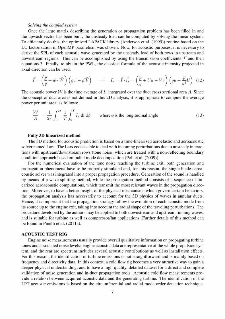