assessment of interruption costs using the weibull...

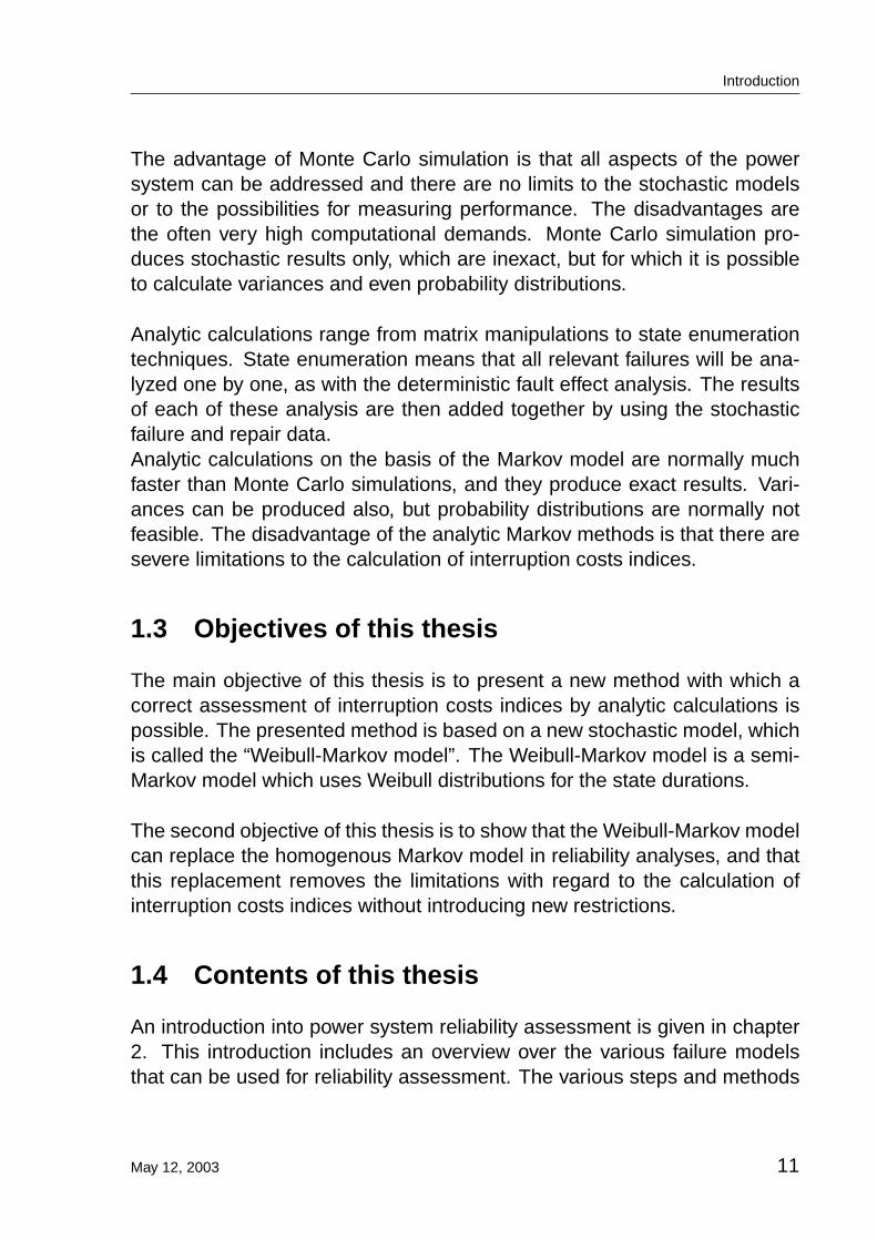
P r 0 1

P r 1 0

P r 1 2P r 2 1

P r 2 0

P r 0 2

h o , b 0

h 1 , b 1

h 2 , b 2

S t a t e 0S t a t e 1

S t a t e 2

Assessment of Interruption Costsin Electric Power Systemsusing the Weibull-Markov Model

JASPER VAN CASTEREN

Department of Electric Power EngineeringCHALMERS UNIVERSITY OF TECHNOLOGY

Göteborg, Sweden, 2003

Thesis for the degree of Doctor of Philosophy

Technical Report No. 381

Assessment of Interruption Costs in ElectricPower Systems using the Weibull-Markov Model

by

Jasper van Casteren

Department of Electric Power EngineeringChalmers University of Technology

S-412 96 Göteborg, Sweden

Göteborg 2003

Assessment of Interruption Costs in Electric Power Systems using theWeibull-Markov Model

© Jasper van Casteren, 2003

Jasper van CasterenAssessment of Interruption Costs in Electric PowerSystems using the Weibull-Markov Model.

Doktorsavhandlingar vid Chalmers tekniska högskola.Ny serie Nr. 1984

ISBN 91-7291-302-9ISSN 0346-718X

Printed in Sweden.

Chalmers ReproserviceGöteborg 2003

Dedicated to Wille

Preface

The liberalization of the electricity markets has increased the need for perfor-mance assessment. The ability to produce qualitative performance indica-tors for an existing or planned power system is essential in order to improveoverall efficiency.

The reliability of supply is directly affected by a reduction in investment. Tocompare the gain in reliability against the required investments, a monetaryevaluation of reliability performance is required. Such is possible by calcu-lating expected interruption costs for groups of customers.

Currently used methods for assessing interruption costs are either slow andinexact, or bare the risk of producing unrealistic results. It was believed thatit would be worth to try for an alternative calculation method that would beaccurate, yet fast, and realistic enough to be practicable.

It was shown in the Licentiate thesis, which was published in February 2001,that an alternative stochastic model had been found in the Weibull-Markovmodel and it was shown that the methods based on that model had potential.

This thesis is based on and contains large parts of the licentiate thesis. Thechapters in which the Weibull-Markov model was introduced are reproducedhere without important changes. It is shown in this thesis that the Weibull-Markov methods and models are a good alternative for the commonly usedhomogenous Markov models.

This Doctor Thesis would not have been possible without the constructivecooperation between Chalmers University of Technology in Sweden andDIgSILENT GmbH in Germany; without the patience of Dr. Martin Schmieg(at DIgSILENT); without the suggestions of Dr. Markus Pöller (at DIgSI-LENT); without the discussions with Math Bollen (my examiner at Chalmers)or without the love of Wille Groenewolt (at home).

Gomaringen, Baden-Württenberg, May 12, 2003,Jasper van Casteren

Abstract

Modern competitive electricity markets do not ask for power systems withthe highest possible technical perfection, but for systems with the highestpossible economic efficiency. Higher efficiency can only be reached whenaccurate and flexible analysis tools are used. In order to relate investmentcosts to the resulting levels of supply reliability, it is required to quantify sup-ply reliability in a monetary way. This can be done by calculating the ex-pected interruption costs.

Interruption costs evaluation, however, cannot be done correctly in all casesby methods which are based on the commonly used homogenous Markovmodel and is time consuming when using a Monte-Carlo simulation. It wasthe objective of this thesis to find a new way for calculating interruption costswhich would combine the speed and precision of the analytic Markov methodwith the flexibility and correctness of the Monte Carlo simulation.

A new calculation method was found, based on a new stochastic model.This new model was called the “Weibull-Markov” model and is described indetail in this thesis. The new model and methods have been implemented ina computer program and the speed and accuracy of the calculation methodwas tested in various projects and by comparison with Monte-Carlo simula-tions.

It is shown in this thesis that disregarding the effects of the probability dis-tribution of the interruption duration can lead to large errors, up to 40 % andmore, in the calculated expected interruption costs. An estimation of thepossible error has been made for a large number of published customer in-terruption cost functions. The actual error in specific reliability calculations ishard to estimate. It is however clear that this error cannot be simply ignored.

The use of the new Weibull-Markov model and the reliability assessmentmethods do not significantly slow down the calculation speed, offer moreflexibility in reliability worth assessment and produce more accurate results.They can be used in all areas of power system reliability assessment whichhave always been the exclusive domain of homogenous Markov modeling.

keywords: power system reliability, reliability worth, semi-Markov model, in-terruption costs, customer damage function, duration distribution.

Contents

1 Introduction 11.1 Quality and Reliability . . . . . . . . . . . . . . . . . . . . . . 31.2 Reliability Assessment . . . . . . . . . . . . . . . . . . . . . . 81.3 Objectives of this thesis . . . . . . . . . . . . . . . . . . . . . 111.4 Contents of this thesis . . . . . . . . . . . . . . . . . . . . . . 11

2 Power System Reliability Assessment 132.1 Basic Scheme . . . . . . . . . . . . . . . . . . . . . . . . . . 132.2 Failure Models . . . . . . . . . . . . . . . . . . . . . . . . . . 152.3 Failure Effect Analysis (FEA) . . . . . . . . . . . . . . . . . . 192.4 Tertiary Failure Effect Analysis . . . . . . . . . . . . . . . . . 282.5 Stochastic Modeling and Interruption Costs Assessment . . . 28

3 Stochastic models 313.1 Stochastic Models . . . . . . . . . . . . . . . . . . . . . . . . 333.2 Homogenous Markov Models . . . . . . . . . . . . . . . . . . 453.3 Weibull-Markov Models . . . . . . . . . . . . . . . . . . . . . 573.4 The Weibull-Markov System . . . . . . . . . . . . . . . . . . . 623.5 Basic Power System Components . . . . . . . . . . . . . . . 70

4 Interruption Costs Assessment 774.1 Reliability Worth . . . . . . . . . . . . . . . . . . . . . . . . . 774.2 Interruption Damage Functions . . . . . . . . . . . . . . . . . 794.3 Use of Damage Functions . . . . . . . . . . . . . . . . . . . . 834.4 Effects of the Interruption Duration Distribution . . . . . . . . 87

i

5 Example 925.1 Description of the Test System . . . . . . . . . . . . . . . . . 925.2 Markov vs. Weibull-Markov Models . . . . . . . . . . . . . . . 1005.3 Monte Carlo Simulation vs. State Enumeration . . . . . . . . 101

6 Conclusions 103

A Analyzed International CDF 105A.1 Australia . . . . . . . . . . . . . . . . . . . . . . . . . . . . . . 105A.2 Canada . . . . . . . . . . . . . . . . . . . . . . . . . . . . . . 109A.3 Denmark . . . . . . . . . . . . . . . . . . . . . . . . . . . . . 113A.4 Great Britain . . . . . . . . . . . . . . . . . . . . . . . . . . . 115A.5 Greece . . . . . . . . . . . . . . . . . . . . . . . . . . . . . . 118A.6 Iran . . . . . . . . . . . . . . . . . . . . . . . . . . . . . . . . 119A.7 Nepal . . . . . . . . . . . . . . . . . . . . . . . . . . . . . . . 121A.8 Norway . . . . . . . . . . . . . . . . . . . . . . . . . . . . . . 123A.9 Portugal . . . . . . . . . . . . . . . . . . . . . . . . . . . . . . 125A.10 Saudi Arabia . . . . . . . . . . . . . . . . . . . . . . . . . . . 125A.11 Sweden . . . . . . . . . . . . . . . . . . . . . . . . . . . . . . 127

B Glossary of Terms 130

ii

Terms and Abbreviations

Terms

MkD kth central moment of D

VD variance of DσD standard variance of DGD(t, τ) remainder CDF for D > tXc Stochastic component cXc,nc nc’th successive state of Xc

Tc,nc nc’th successive epoch at which Xc changesDc,i duration of Xc = iλc,ij homogenous transition rate for Xc = i to Xc = jλc,i homogenous state transition rate for Xc = iS Stochastic systemSns ns’th successive state of STns ns’th successive epoch at which S changesXc,ns Xc according to Sns

Xc,s Xc according to S = sDc(ns) Remaining duration of Xc,ns at Tns

Ac(ns) Passed duration of Xc,ns at Tns

ηc,i Weibull form factor for Xc = iβc,i Weibull shape factor for Xc = iMc,i Mean duration of Xc = iVc,i Variance of the duration of Xc = i?c,ns = ?c,i for Xc,ns = i, i.e. ηc,ns , βc,ns , etc.?c,s = ?c,i for Xc,s = i, i.e. ηc,s, βc,s, etc.Frc,i Frequency of occurrence of Xc = iPrc,i Probability of occurrence of Xc = iFrs Frequency of occurrence of S=sPrs Probability of S=s

iii

Abbreviations

TTF Time To FailureTTR Time To RepairMTBF Mean Time Between FailuresTBM Time Between MaintenanceCDF Cumulative Density FunctionPDF Probability Density FunctionSF Survival FunctionLPEIC Load Point Expected Interruption CostsECOST Expected Customer Outage Cost

iv

Chapter 1

Introduction

In Western Europe, the availability of electric energy has been long regardedas a basic provision for economic development and prosperity. Centralizedand monopolistic companies were therefore formed to design, construct andcontrol the electrical power systems. These companies strove for technicalperfection in a growing market where the risk of over-investment was consid-ered low. Consequently, the electrical power systems in this part of the worldare among the most reliable and well designed. Fig.1.1 shows some valuesfor the unavailability of the electricity supply, expressed in average minuteslost per year ([45]). This figure shows large differences between variousEuropean countries. Where the average non-availability of electricity in Italyis around 200 minutes per year, it is about 25 minutes in the Netherlands.However, the probability of being not supplied in Italy is still very small andequals 200/(8760*60)=0.00038. This means that electric power is availablein 99.962 % of time. In the Netherlands and Germany, where the averagenon-availability is less than 25 minutes per year, the availability is more than99.995 % of time. This is astonishingly good, considering that we talk abouta very large and complex technical system.

However, modern competitive electricity markets are believed to no longerdemand for power systems with the highest technical perfection, but for theeconomically most efficient. The liberalization of the electricity markets thatresulted from this believe has since forced electric companies to find a newbalance between technical perfection and maximum profit.

May 12, 2003 1

Introduction

Average customer minutes lost per year

0

50

100

150

200

250

300 1996

1997

1998

1999

Italy Norway Sweden UK France Netherlands

Figure 1.1: European Comparison of unavailability

A perfect power system is a power system where all loads are continuouslysupplied by electricity of constant nominal voltage without any waveformdistortion. Of course, such systems do not exist. All loads will suffer supplyinterruptions sometimes, the voltage or current will always show deviationsfrom nominal values and waveforms will always be distorted to some extent.The question is how bad this is. What levels of imperfection can be toler-ated? At which levels will we have the highest achievable efficiency? Highlevels of perfection can only be reached by high investments and will thuscause high prices. Low levels, however, will lead to all kind of costs due toinsufficient performance, such as ([45]) :

• Economic penalties payable to affected customers or into funds.

• Tariff reductions or other revenue affecting penalties by regulating.

• Customer loss due to negative publications.

The liberalization of the electricity markets forces the electricity companiesto view their power plants, transmission networks and distribution systemsin a new light. In order to survive in the open market, it is required to reducecosts and to maximize returns on investments.

2 May 12, 2003

Introduction

It is the task of reliability engineers to support the decision processes in theplanning phases by providing power system performance indicators. Invest-ments can then be judged by the gain in performance.The calculation of (expected) performance indicators in respect to supplyreliability can be divided into the calculation of non-monetary interruptionstatistics and reliability worth assessment. Reliability worth assessment pro-duces monetary indices, and is a relatively young discipline.

This thesis introduces a new stochastic model which can be used to producemonetary indices more correctly, in a fast analytic way, based on a flexibledefinition of damage caused by customer interruptions.

1.1 Quality and Reliability

Electric power is used by consumers to operate electrical machines and ap-pliances. When that is possible without exceptions, then such consumerswill be satisfied and we have sufficient power quality . Power quality is thusa measure for the ability of the system to let the customers use their electri-cal equipment. Any peculiarity or fault in the power system that (might) pre-vent the use of electrical devices or (might) interrupt their operation meansa lack of power quality.

The ability of the system to let customers use their equipment is determinedby the extent to which the voltage and/of the current of the consumer’s powersupply are ideal. All deviations from the ideal are called power qualityphenomena or power quality disturbances. A power quality phenomenoncan be a sudden change of values, a limited period of lesser quality, but alsoa continuous situation in which some (sensitive) equipment can not be usedproperly.

Continuous or slow changing offsets from a perfect power quality are calledvoltage variations or current variations. Phenomena which suddenly appearand which have a limited duration are called power quality events.

In [30], an exhaustive description of power quality variations and events isgiven. Possible power quality variations are:

May 12, 2003 3

Introduction

• Voltage/current magnitude variations

• Voltage frequency variations

• Current phase variations

• Voltage and current unbalance

• Voltage fluctuations (“flicker”)

• Harmonic distortion

• Interharmonic components

• Periodic voltage notching

• Mains signaling voltages

• High frequency voltage noise

and some example of power quality events are:

• Interruptions

• Undervoltages

• Overvoltages

• Voltage magnitude steps

• Voltage sags

• Fast voltage events (“transients”)

Power quality variations, as listed above, are examples of the voltage qual-ity or current quality of the electric supply. Power quality variations, how-ever important and interesting, are not further considered in this thesis.

The power quality events can be divided into two groups:

• Interruptions

• Other voltage quality events

4 May 12, 2003

Introduction

Depending on the duration of the event, momentary, temporary and sus-tained interruptions can be distinguished. Reliability analysis is the field ofresearch which calculates the number and severity of power interruptions.It is divided into the field of security analysis and adequacy analysis. Secu-rity analysis calculates the number of interruptions due to the transition fromone situation to the other. Adequacy analysis looks at interruptions whichare due to the non-availability (“outage”) of one or more primary componentsin the system. The position of adequacy analysis in the whole area of powerquality analysis is illustrated by Fig.1.2.

U n d e r - , O v e r v o l t a g e sV o l t a g e m a g n i t u d e s t e p s

F a s t v o l t a g e e v e n t sV o l t a g e s a g s

P o w e r Q u a l i t y

P o w e r Q u a l i t yE v e n t s

P o w e r Q u a l i t yV a r i a t i o n s

I n t e r r u p t i o n s

D u e t o O u t a g e

D u e t o T r a n s i t i o n

R e l i a b i l i t y A s s e s s m e n t

S e c u r i t y A n a l y s i sA d e q u a c y A n a l y s i s

Figure 1.2: Power Quality and Adequacy Analysis

The subject of this thesis is power system adequacy analysis. Security anal-ysis is not further addressed.

May 12, 2003 5

Introduction

One method for determining the number of interruptions is by monitoringvoltages and counting the number of interruptions.For the use of deciding, from the monitored voltages, when an interruptionsoccurs, a criterion like the one in the IEEE std.1159-1995 can be used.This standard defines an interruption as an event during which the voltageis lower than 0.1 p.u. A sustained interruption is defined as an interruptionwith a duration longer than 1 minute.

When monitoring a real power system we normally have the situation that allkinds of events can cause interruptions, but that the exact causes for spe-cific captured interruptions are often unknown. That is why some minimumvoltage like 0.1 p.u. is required as criterion for an interruption. A criterion like“not longer connected to a source of electric power” cannot be used for mea-surements, as the network condition is normally unknown when classifyingthe voltage measurement.

A completely different situation occurs when reliability calculations are madewith a computer program using digital network models. In that case, onlya very specific set of events will happen, namely only those events whichhave been modeled. For each analyzed interruption, it is known in detailwhy the interruption occurred and the status of all parts of the power systemis completely known. On the other hand, a voltage at the interrupted loadpoints is normally not calculated. That is why we need a different definitionfor an interruption when we perform reliability analysis.

For the purpose of the assessment of reliability indices by system modelingand mathematical analysis, it can be assumed that as long as a customeris still physically connected to the power system, he will be supplied. Onlywhen a customer is disconnected from the system, it is called an interrup-tion.

The interruptions of customers are caused by failing equipment, or by main-tenance which is performed to prevent equipment from failing. Failures areevents where a device suddenly does not operate as intended, and failuresoccur in all parts of the power system. Cables are damaged, for example,by digging activities, lighting strikes, breakers suddenly open, transformers

6 May 12, 2003

Introduction

burn out, etc., etc. Every reliability analysis must start by recognizing andmodeling all relevant failures which may affect the system’s reliability.

A failure, or a possible future failure, may lead to the temporarily removal ofone or more primary devices from the system. The situation where a primarydevice is removed is called an outage and the removed device is said to be‘outaged’. An outage will bring the system in a weakened condition.

Primary devices are removed in order to clear a fault, to prevent further dam-age or weakening of the system, to repair a faulted device or for performingmaintenance. All equipment that is de-energized or isolated is said to beoutaged. Not all outages result from failures, however, and not all failureswill lead to outages. When devices are deliberately removed from the sys-tem for preventive maintenance, then that is called a “scheduled outage”or “planned outage”. An outage which is an inevitable result of a failure iscalled a “forced outage” or “unplanned outage”.

Outages may lead to situations in which customers are not longer suppliedwith electric power. As mentioned before, such an event is called an in-terruption. Not all outages will lead to interruptions. Many components,especially at higher voltage levels and in industrial systems, are operated inparallel. After the outage of one component, the parallel one will take overimmediately and the load or customer will not experience an interruption.The reserve capacity of a power system which is used to compensate for anoutage is called “redundancy”. Redundancy improves the reliability.

Besides causing interruptions, outages may also affect the system’s ability toperform scheduled transports of power without violating technical or opera-tional constraints. Often, outages in meshed high-voltage transport systemswill not lead to interruptions, but they generally affect the transport capaci-ties. Outages in radially operated distribution systems on the other hand willnormally not affect transport capacity, but will often lead to interruptions.

The relation between failures, outages, interruptions and reduced transportcapacity is shown in Fig.1.3

May 12, 2003 7

Introduction

F a i l u r e

O u t a g e s

I n t e r r u p t i o n sD e c r e a s e d

T r a n s p o r t C a p a c i t y

N o O u t a g e s

N o E f f e c t s

Figure 1.3: Failures and possible results

1.2 Reliability Assessment

Reliability assessment, although targeted at only one aspect of power qual-ity, is nevertheless a wide area itself. Three basic types of reliability assess-ment can be recognized:

• Monitoring of system performance

• Deterministic reliability assessment

• Stochastic reliability assessment

The monitoring of system performance is performed by capturing the num-ber, type and duration of interruptions. This is indispensable for gatheringdetailed information about the performance of power system components. Itis also used for bench-marking purposes which are, for instance, used formarket regulating.

System performance monitoring, however, can normally not be used to as-sess the reliability of individual parts of the networks. The size of such net-works is often so small that years of monitoring would be required in orderto reach some statistical significance. Of course, it can also not be used tocompare design alternatives for system expansion planning.

8 May 12, 2003

Introduction

Deterministic reliability assessment can be based on active failures (faults)or on outages. Deterministic outage-based reliability assessment will per-form an outage effect analysis for each relevant outage in the system. Eachoutage may cause the interruption of one or more loads or may cause over-loading of parallel parts of the system. The well-known “n-1”, or “n-k”, anal-ysis is an example of such analysis. Deterministic outage-based reliabilityassessment produces qualitative results, telling if criteria are met or not, butmay also produce quantitative results such as capacity margins, maximumloading, maximum interrupted power, etc.

Deterministic fault-based reliability assessment does not analyze the effectof outages, but the effects of faults (active failures). The difference is thatthe reactions of the power system are considered in a fault effect analysiswhereas they are neglected in an outage effect analysis. Typical systemreactions to a fault are (in chronological order)

• Fault clearance by protection

• Fault isolation

• Power restoration

A fault effect analysis may produce several sets of outage conditions, eachwith a different duration. Each of these conditions will be analyzed for inter-ruptions and overloads. More detailed criteria can then be used to judge theadequacy of the system. It may, for instance, be acceptable to have someinterruptions as long as power to the interrupted loads can be restored within30 minutes, or short-term overloading can be tolerated. Such criteria cannotbe tested with an outage effect analysis only.

Stochastic reliability assessment adds to a deterministic fault-based reliabil-ity assessment in two aspects:

• It may also consider passive failures

• It uses stochastic failure models

The use of stochastic models allows the calculation of averaged indices, bycombining the results of the various failure effects analysis on the basis ofthe failure frequencies and/or probabilities.

May 12, 2003 9

Introduction

Stochastic failure models define the expected number of times a failure willhappen per unit of time, and how long it will take to repair the failed com-ponent. During the repair, the failed component will be out of service, andall customers which cannot be supplied without the component will be inter-rupted for the duration of the repair. Mathematical expressions are usedto calculate the probability or the severity of the interruptions, using thestochastic failure data. The possibilities for calculating interruption sever-ity depend on the used stochastic model. If the severity depends not only onthe mean interruption duration, but also on the probability distribution of theduration, then the commonly used homogenous Markov models complicatesuch severity calculations. The new Weibull-Markov model, to be introducedin chapter 3 of this thesis, is more suited for calculating interruption severityindices.

In stochastic reliability assessment, each relevant failure is analyzed in afailure effect analysis (FEA). A typical FEA uses a multitude of power systemanalysis tools, such as

• topological analyses for finding isolated areas, power restoration swit-ches, etc.

• loadflow calculations for overload detection

• linear optimization tools for overload alleviation

• short-circuit analysis for fault clearance

• interruption costs calculations

The combination of the results of the performed FEA’s into averaged results,on the basis of the stochastic data, is currently done in roughly two ways

• By Monte Carlo simulation

• By analytic calculations, using Markov models

Monte Carlo simulation is the repeated chronological simulation of the powersystem. During each simulation, faults will occur randomly, as in real-life,and the reactions of the system to these faults is simulated chronologically.The performance of the system is then monitored during the simulations.

10 May 12, 2003

Introduction

The advantage of Monte Carlo simulation is that all aspects of the powersystem can be addressed and there are no limits to the stochastic modelsor to the possibilities for measuring performance. The disadvantages arethe often very high computational demands. Monte Carlo simulation pro-duces stochastic results only, which are inexact, but for which it is possibleto calculate variances and even probability distributions.

Analytic calculations range from matrix manipulations to state enumerationtechniques. State enumeration means that all relevant failures will be ana-lyzed one by one, as with the deterministic fault effect analysis. The resultsof each of these analysis are then added together by using the stochasticfailure and repair data.Analytic calculations on the basis of the Markov model are normally muchfaster than Monte Carlo simulations, and they produce exact results. Vari-ances can be produced also, but probability distributions are normally notfeasible. The disadvantage of the analytic Markov methods is that there aresevere limitations to the calculation of interruption costs indices.

1.3 Objectives of this thesis

The main objective of this thesis is to present a new method with which acorrect assessment of interruption costs indices by analytic calculations ispossible. The presented method is based on a new stochastic model, whichis called the “Weibull-Markov model”. The Weibull-Markov model is a semi-Markov model which uses Weibull distributions for the state durations.

The second objective of this thesis is to show that the Weibull-Markov modelcan replace the homogenous Markov model in reliability analyses, and thatthis replacement removes the limitations with regard to the calculation ofinterruption costs indices without introducing new restrictions.

1.4 Contents of this thesis

An introduction into power system reliability assessment is given in chapter2. This introduction includes an overview over the various failure modelsthat can be used for reliability assessment. The various steps and methods

May 12, 2003 11

Introduction

that are used for the failure effect analysis (FEA) are discussed in chapter2.3. Stochastic models are introduced in chapter 3. This chapter covers thebasics of homogenous Markov models and introduces the Weibull-Markovmodel. Interruption costs assessment is discussed in chapter 4. Chapter 5discusses the results for an example distribution network.

12 May 12, 2003

Chapter 2

Power System ReliabilityAssessment

2.1 Basic Scheme

The assessment of the reliability of a power system means the calculationof a set of performance indicators. An example of such an indicator is theLPAIF, or the "Load Point Average Interruption Frequency", which equals theaverage number of times per year a load point suffers an interruption. Twodifferent sets of indicators can be distinguished: local indicators and systemindicators. Local indicators are calculated for a specific point in the system.Examples are

• The average time per year during which a specific generator is not ableto feed into the network

• The average duration of the interruptions at a specific busbar.

• The interruption costs per year for a specific customer.

System indicators express the overall system performance. Examples are

• The total amount of energy per year that cannot be delivered to theloads.

• the average number of interruptions per year, per customer.

• The total annual interruption costs.

May 12, 2003 13

Power System Reliability Assessment

Power system reliability analysis can be split into three parts:

1. The definition of a model for the healthy, undisturbed, power system.

2. The definition of possible deviations from the healthy system state,such as possible failures, changes in demand, planned outages, etc.

3. The analysis of the effects of a large set of healthy and unhealthy sys-tem states.

The results of the analyses of the various system states is used to calculatethe performance indicators. The basic diagram of the calculation procedureis depicted in Fig.2.1.The definition of the initial healthy system state is the starting-point of thereliability assessment procedure. In this system state, all components areworking as intended. The initial load profile, generator dispatch and switchsettings allow for a normal, healthy, loadflow in which no overloading or volt-age deviations should be present.

The set of definitions of possible deviations from the initial state is used togenerate events. These events will bring the system in an disturbed state,such as may occur in the real system. This disturbed state is then processedby the failure effect analysis, which may react to present faults or other unde-sirable situations by opening switches, restoring power, performing repairs,or other changes to the system. This is repeated until enough unhealthysystem states have been analyzed. Finally, the intermediate results are pro-cessed to produce the various performance indicators.

In order to perform a reliability assessment, we thus have to creates modelsfor the various failures and other disturbances that that may occur in thesystem. Secondly, we have to be able to analyze the effects of these systemdisturbances. Thirdly, we have to select the relevant system conditions andfailures that must be analyzed in order to calculate the reliability performanceindicators.

The various failure models and the methods to select relevant system statesare described in the following sections. The Failure Effect Analysis is thesubject of the next chapter.

14 May 12, 2003


initial healthy, undisturbed, state

failures planned outages demand changes

Failure Effect Analysis

results

operational, disturbed, state

repairs reconfigurations dispatch

react

no yes

More States ?

Figure 2.1: Basic reliability assessment scheme

2.2 Failure Models

Failures in power systems can be divided into active and passive failures.Active failures are failures that require an automatic intervention of protec-tion devices. Passive failures will not directly provoke a reaction of the powersystem. Some passive failures will remain undetected until an inspection iscarried out or until the device is called upon to perform its function.

2.2.1 Passive Failures

Passive failures may persist in the system for a long time without furtheraffecting the system. Although they may cause the interruption of customersin some cases, they are seldom a direct threat to the system itself. Thereaction time to passive failures is therefore in the range of minutes to hoursor even days to months.

Passive failures can be divided into manifest failures and hidden failures.Manifest failures will show themselves directly in their effects, where hidden

May 12, 2003 15


failures can exist undetected up to the next inspection or up to the momentthe component is called upon.

Manifest Failures

The following manifest failures can be distinguished:

• Inadvertent breaker opening (mal trip). A mal-trip can occur in fourways:

– Independent inadvertent breaker open. This is the sudden open-ing of a breaker either due to a human error, a breaker failure oran automation failure. The occurrence of these failure is indepen-dent of the existing state of the network.

– Independent mal-trip. This is the incorrect opening of a breakerby a protection device without a short-circuit in the system.

– Maintenance related inadvertent breaker open. This may happendue to incorrect switching in relation to maintenance where, forinstance, backup-equipment is taken out inadvertently.

– Fault-related mal-trip. This is the incorrect opening of a breakerby a protection device in relation to an existing short-circuit.

• Independent Equipment Trip Independent equipment trips are sud-den outages primary components due to a fault in the component itself.Examples are generator trips due to turbine faults or the tripping of aBuchholz-relay at a transformer.

Hidden Failures

Hidden failures will cause the failed component to not perform the next timeit will be called upon to function. Examples are undetected relay failures,undetected communication channel failures and stuck breakers.

2.2.2 Active Failures

Active failures are a direct threat to the power system. They may lead to se-vere damage and even total system collapse when they are not immediately

16 May 12, 2003


cleared. It is the task of automatic protection equipment to react to activefailures and to minimize direct damage to the system.

Four kinds of active failures can be distinguished:

• Single active short-circuits.

• Cross Country faults.

• Common mode faults.

• Overlapping faults.

Single Active Short-Circuits

A single active short-circuit is a fault at a single location which leads to theimmediate isolation of the faulted area by automatic protection devices. Thefault may be either a three-phase, a two phase, a two phase with earth or asingle phase short-circuit.

In compensated networks, it is possible to operate the network with a single-phase short-circuit long enough to allow for load transfer or other preventivesystem reconfigurations. Such is done in order to isolate and repair the faultwithout or with a minimum of customer interruptions. The only contributionof such single phase failures to the unreliability would then be the reducedredundancy during the repair and the risk of inadvertent switching in relationto the network reconfigurations and repair.Single phase short-circuits in compensated networks which do not lead toautomatic protection intervention or load interruptions can be neglected in areliability assessment.

Cross Country Faults

A cross-country failure starts with a single phase fault in a compensated net-work, which is not isolated by protection. Due to the presence of the singlephase fault, the voltage at the other phases is raised by a factor of

√3. This

increased phase voltage may lead to a second short-circuit somewhere elsein the network, after which one or both failures will be isolated by automaticprotection intervention. The double short-circuit is called a cross countryfailure.

May 12, 2003 17


Common Mode Failures

A common mode failure is the simultaneous occurrence of two or more ac-tive failures due to a single common cause. A common mode failure will leadto the immediate isolation of all areas which contain the faults. Examples are

• lightning flash-over at multi-circuit towers

• damage to multi-circuit poles or towers due to car accidents

• multiple cable damage due to excavation works

Overlapping Faults

An overlapping fault is a fault which occurs during the outage of one or morerelevant other components. These other components may be on forced out-age, i.e. on repair, or on planned outage, i.e. during maintenance.

Important is that the outaged components are relevant to the faulted com-ponent. For the power system of Sweden, for example, it is likely that somerepair or maintenance is going on somewhere at any time. That would meanthat all faults in Sweden will happen during one or more forced or plannedoutages, and all faults in Sweden would therefore be “overlapping faults”.That would make no sense.In defining overlapping faults, only those outages are regarded which causea significant difference in the effects of the occurring fault. In the case oftwo parallel transformers, we would have an overlapping fault if the secondtransformer fails during the outage of the first. The outage of the first trans-former is relevant, because this could mean that customers are interruptedwhere they would not have been when both transformers were available. Inother cases, the occurrence of an overlapping fault could also mean thatpower is restored slower because relevant equipment is not available.

The problem with detecting relevant pre-fault outages is that we would haveto make a failure effects analysis in order to find out that we do not need toanalyze the combination of outage and fault. That would be to late, as wewould already have analyzed it.

18 May 12, 2003


Another aspect of pre-fault outages is that they will change the operationalstate of the network. This normally leads to higher loading of backup equip-ment, which may lead to higher failure rates. Such accelerated faults due topre-fault outages always lead to overlapping outages, as it is clear that theoutaged and the faulted component are not independent.

This can also be generalized : we could detect at least a subset of all possi-ble faults for which a certain outage is relevant by calculating the differencein pre-outage and during-outage loading of all components. Those com-ponents which show a significant difference in loading are affected by theoutage and therefore good candidates for an overlapping fault analysis.

Overlapping faults differ from common mode failures because they do notoccur at the same time. More important is that overlapping faults are oftenmuch more seldom than common mode failures, because their frequencyof happening is the product of failure frequency and the probability of thepre-fault outage, which normally is very low.

This can be shown with the simple example of two parallel cables. Supposethe independent failure frequency for each cable is once every 5 years =0.2/a, and that a repair takes 10 hours on average. The probability of beingin repair for each cable is thus 10h · 0.2/a = 2h/a = 2/8760. A year of 8760hours is used here, which is common practice in reliability assessment. Thismeans that an overlapping failure will occur

2 · 28760

· 0.2/a =1

10950/a (2.1)

i.e. once in 10950 years on average. The frequency for a common modefailure due to digging, for example, is often much higher than that.

2.3 Failure Effect Analysis (FEA)

The task of the Failure Effect Analysis (FEA) is to analyze the ability of thesystem to provide all loads with sufficient power after a failure, without violat-ing the system constraints. If not all loads can be supplied with power, thenthe loads which suffer an interruption have to be identified, as well as theduration of these interruptions. The FEA is a quasi steady-state analysis.

May 12, 2003 19


Load interruptions due to the transient effects of the sudden introduction ofshort-circuits and the subsequent opening and closing of switches, are notconsidered here. Such transient effects are the subject of security analysis.

The FEA not only comprises the analyses of steady-state system states, butalso includes the simulation of the reactions of the system and the systemoperators to faults and other emergency situations. The power system isactively changed during such a simulation, which may include

• switching actions in order to clear and isolate faults

• switching actions in order to restore power

• switching actions, re-dispatch and load shedding in order to alleviateoverloading

The Failure Effect Analysis is a mixture of short-circuit analyses, load flowcalculations, topological analysis and system simulation. The level of detailin the FEA is determined by the level of detail in these sub-analyses andsimulations, and so is its complexity and calculating speed.

The output of the FEA is a list of busbars and terminals which are interrupteddue to the failures in the analyzed operational state, each with a descriptionof the duration of these interruptions. These descriptions can be a singlevalue in case of a deterministic duration, or a probability distribution in caseof a stochastic duration.

The input data required for performing the FEA are

• the basic system definition

• the operational system state

• the failures in the system

The FEA thus starts with a system in which one or more, possibly active,failures may be present.

The basic system definition includes all aspects of the power system whichare assumed constant during the reliability assessment, which comprises:

20 May 12, 2003


• the topology of the system

• the electrical models for all primary equipment

• the models of all relevant protection devices

• all relevant loadflow controller models, such as

– secondary controllers

– voltage controllers, tap changer controllers

– shunt and VAR compensator controllers

• emergency and maintenance switching protocols

The topology of the system is considered here independent of switch po-sitions. The position of a switch, either open or closed, does therefore notchange the basic topology. Also, any possible connection or generator whichmay be used in certain emergency conditions, i.e. for restoring power to im-portant loads, must be defined as a part of the basic system topology.The electrical models must be accurate enough to allow a valid loadflowcalculation.

The operational system state comprises

• the set of forecasted peak load profiles

• the set of forecasted peak transport flows

• switch positions

• generator availabilities and capacities

• planned outages

• ongoing repairs

Each FEA starts by changing the system model to the current operationalstate, and then introduces one or more failures. The effects of these failuresis then analyzed in three phases:

• Primary Failure Effect Analysis

• Secondary Failure Effect Analysis

• Tertiary Failure Effect Analysis

May 12, 2003 21


2.3.1 Primary Failure Effect Analysis

The primary failure effect analysis determines the effects of the automaticreactions of the power system to the active failures, i.e. the reactions of thesystem’s automatic protection devices, such as over-current relays, fuses,distance relays, under-voltage or over-voltage relays, under-frequency re-lays, etc.The results of the primary reactions are the opening of one or more breakersin the system. Typical reaction times are in the order of milliseconds to afew seconds. Due to these short reaction times, the primary failure effectscannot be prevented or modified after the occurrence of the failures. Theobjective of the primary reactions of the power system are to minimize thedamage and to minimize the direct effects of the fault to non-faulted parts ofthe system.

All active failures must be cleared by the protection. To find out which re-lays will intervene, a short-circuit calculation is needed. The advantagesof using short-circuit analysis is that fault currents can be established, andprotection selectivity can thus be regarded. The disadvantage is that short-circuit analysis requires detailed overcurrent, differential and distance relaymodels. For many reliability assessment projects, such detailed informationis not available, mostly because the reliability assessment is required in astage of project development where the protection system has not been de-signed yet. Another argument against the use of full short-circuit calculationis the calculation speed. But even in cases where calculation speed is nota problem and detailed protection data is available, the use of short-circuitanalysis could complicate the interpretation of the results, because both theprimary and secondary system design would have to be regarded.

If perfect selectivity can be assumed, then a fast topological analysis canbe used to simulate fault clearance. Instead of performing a short-circuitcalculation, a topological search algorithm is started at the fault position.This algorithm will continue to search the network around the fault positionup to the first relays. The smallest area around the fault which can be iso-lated by protection devices is thus found. These protection devices are thenassumed to trip. The advantage of this method is, besides its speed, theminimum requirements on the protection modeling. The only required infor-mation is the position where protection devices are measuring fault currents

22 May 12, 2003


and which breaker(s) they will open. In the case of a fuse, only the locationis required, and this is also true for many overcurrent and distance relays.This limited demand for relay information makes it possible not only to start areliability assessment in an early stage of system design, but also to quicklycompare various basic protection system lay-outs.

1

a

b a

a

a

b

b

b b

Figure 2.2: Cleared area and backup protection

In Fig.2.2, a part of a network is shown in which a short-circuit occurs. Thetopological search algorithm will find the dotted area as the smallest areathat can be isolated in order to clear the fault. The relays at “1” are found asthe relays that will trip. As the faulted area is fed from two sides, two relayshave to be tripped. Breaker fail-to-trip, as would happen when a hiddenfailure is present in the relay or the breaker, can be accounted for by notopening the breaker and letting the topological algorithm search further. InFig.2.2, it is assumed that the upper breaker at “1” fails to trip. The nextsmallest area to clear is by tripping the breakers at the parallel transformers.The tripping of these backup relays will mean a prolonged fault clearancetime and the whole area in Fig.2.2 will be tripped.

For the purpose of reliability assessment, the fault clearance time is not im-

May 12, 2003 23


portant. Important is, however, the fact that a much wider area is tripped andthus more customers are interrupted than without the hidden failure whichled to the fail-to-trip event. If we assume a failure frequency for the fault inFig.2.2 of F (1/a), and a fail-to-trip probability of P = Ps + Pr, with Ps forthe breaker and Pr for the relay, then we will have a contribution to the inter-ruption frequency for the loads “a” in Fig.2.2 of F (1/a) and a contribution ofP · F (1/a) for the loads “b”.

Important is that the short-circuit itself, i.e. the system state directly after theshort-circuit appears and before the first protection devices intervene, is notregarded. The short-circuit itself and the detailed analysis of fault currents,remaining voltages and fault clearance times, including the effects of fail-to-trip events and backup protection, is the subject of voltage sag analysis.

2.3.2 Secondary Failure Effect Analysis

The secondary failure effect analysis considers the reaction of the powersystem and its operators to the condition which is reached after the primaryreaction has finished. Typical durations for the secondary reactions are inthe order of seconds to minutes for automatic reactions and in the orderof minutes to hours for manual reactions. The objective of the secondaryreactions are to minimize the duration of the interruptions and to alleviateany violated operational constraint.

Fault Isolation and Power Restoration

The task of the primary FEA is to clear active failures by isolating the small-est possible area containing the fault. The area which is isolated to clearthe fault is called the “cleared area”. All loads in the cleared area will sufferan interruption. It is the task of the fault isolation and power restoration tosimulate the process of fault location, fault isolation, power restoration andrepair. This is done by searching for the smallest possible area around thefault and subsequently restoring power to as many customers as possibleand as quickly as possible ([57]). Fig.2.3 illustrates this process. The shownfault in this schematic example will lead to the isolation the whole bottomfeeder by protection. This is the “cleared area”. By manually opening two

24 May 12, 2003


isolators, the fault can be isolated more selectively. Power to the remainingparts of the cleared area can then be restored and these areas are there-fore called “restorable areas”. Areas that are actually restored by (re)closingswitches are called “restored areas”.

O p e n /C l o s e

C l o s e

f a u l t e da r e a

r e s t o r e da r e a

r e s t o r e da r e a

c l e a r e d a r e a

Figure 2.3: Cleared, faulted and restored areas

The fault isolation uses the same topological search for switches as hasbeen used for the fault clearance. A topological search is started at thefaulted components to find the smallest area that can be isolated in orderto isolate the fault. However, in stead at protection devices, the search nowstops at any switch that can be opened.

The faulted area is smaller than or equal to the cleared area. The areas be-tween the faulted and the cleared area are the “restorable areas” because,principally, power may be restored to the customers in these areas. The ac-tual power restoration is performed by finding all switches that can connector reconnect a restorable area to a supplied area. One or more of theseswitches are then closed to restore power.

Important for the power restoration scheme is that the resulting interruptiontimes are realistic. The used method must, for instance, regard the effects

May 12, 2003 25


of remote sensing and switching. The interruption duration in the case of“switched” power restoration, i.e. in the case of power restoration by networkreconfiguration, is determined by the time spend locating the fault, the timerneeded to open the switches that isolate the fault and the time needed todetermine and close the switches through which the power is restored. Eachof these times depend on the amount of automation and remote control inthe network, the presence of short-circuit detectors, the type of relays, theloading of the network, the accessibility of sub-stations, etc.

After the fault isolation and power restoration phase have finished, the net-work will be reconfigured and power flow will be different from the pre-faultsituation. In some cases, for instance in many low voltage distribution net-works, it can be assumed that overloading in the post-fault situation doesnot occur. Overload verification can then be omitted, thus increasing thecalculation speed. A simple connection algorithm is used to check if a loadis still physically connected to a generator or external network. When so, theload can be considered to be supplied.

In many cases, overloading can not be disregarded. This is especially thecase in meshed transmission networks, or highly loaded distribution sys-tems. Some kind of overload verification must then be used.

Overload Alleviation The observed overloads have to be alleviated. Theway in which this is done depends on the system condition, the fault thatcaused the overloading, and on the type of overloading. Overload alleviationmay include

• switching-in backup equipment and cold reserve,

• maintenance or repair cut-off, which means that components whichare currently on outage are brought back into service as fast as possi-ble,

• network reconfiguration,

• generator re-dispatch,

• load reduction, load transfer and load shedding.

26 May 12, 2003


These three methods are listed in order of applicability. Load shedding isa last-resort method when everything else fails. Load shedding will leadto customers interruptions. These interruptions, although caused by oper-ator intervention, must be looked upon as forced interruptions, and not asplanned interruptions. The frequency and duration of load shedding there-fore must be added to the interruption statistics.

Linear programming techniques are often used to find the switches to openor close, the generators to change or the loads to reduce, transfer or shed.These optimization techniques try to minimize the effects of the overloadson the customers and are normally based on some linear network flow cal-culations.

In the case of (sub-)transmission reliability assessment, some load may betransferred from one feeder to the other by switching actions in the distribu-tion networks. These networks, however, may only be included in the trans-mission model as single lumped loads. In that case, load transfer must bemodeled by stating ‘transferable’ percentages and transfer targets for spe-cific loads. The transfer targets are the loads to which the given percentageof power is transferred.

2.3.3 Manipulation of the Secondary FEA

The emergency reconfiguration schemes for fault isolation and power resto-ration normally have a significant effect on the calculated reliability indices.By correctly locating and isolating the fault and subsequent closing of normal-ly open switches, the interruption duration can often be drastically reduced.Improving the supply reliability by improving the emergency reconfigurationschemes, however, is only feasible when it is possible to associate the im-pact of a fault with specific schemes. It must then be possible to analyze,adjust and check these schemes in detail.It is therefore important to model the fault isolation and power restorationschemes in a way that they

• reflect reality

• allow fast modifications and experiments

• are transparent and can be checked easily

May 12, 2003 27


• allow for further investigations

The outcome of the secondary FEA is a list of interrupted loads with theduration of the interruptions. This duration will be deterministic in the caseof a “switched” power restoration, i.e. in the case of power restoration bynetwork reconfiguration. When switched power restoration is not possible,the faulted components have to be repaired in order to restore power. Such“repaired” power restoration will have a stochastic duration.

But even when we assume switched restoration to have a deterministic du-ration, then we often still have a different interruption duration for differentloads in different restored areas. Another difference in interruption durationoccurs when some loads have to be shed at once, while others will be shednot before some short-term overloading limit is violated.

It is obvious that the implementation of the secondary FEA will have a sig-nificant influence on the produced reliability indices. In [41], a method isdescribed in which power restoration schemes for specific failures can bedefined in an interactive way.

2.4 Tertiary Failure Effect Analysis

Typical reaction times for tertiary reactions are in the order of minutes tohours. The objective of the tertiary reactions are to optimize the operationalstate which is reached after the secondary reactions have finished. Tertiaryreactions are not considered further in this thesis.

2.5 Stochastic Modeling and Interruption Costs As-sessment

In order to produce qualitative reliability indices for a power system, we haveto provide both electric system data and component failure data.With the electric system data and the component failure data, contingenciescan be created, i.e. system states in which one or more failures are present.A failure effect analysis, including a primary, secondary and tertiary FEA, is

28 May 12, 2003


then performed. The FEA produces a list of interrupted customers and willalso calculate the duration of the interruption for each individual customer.

The duration is a very important aspect of the interruption, and its meanvalue can be used, for instance, to calculate the annual interruption proba-bility, expressed in minutes per year of not being supplied. It depends onthe type of the used failure models if it will also be possible to calculate theprobability distribution of the interruption duration for a specific contingency.As the failure models use stochastic durations, i.e. stochastic life-times andrepair durations, a repetition of the same contingency under the same con-ditions will lead to different interruption durations. The interruption durationis therefore a stochastic quantity.

This is important because the damage caused by an interruption will oftendepend largely on the duration of the interruption. If this dependency is notlinear, then it will not be possible to calculate the expected interruption costscorrectly when the probability distribution of the duration is not known.

s y s t e m d a t a

W e i b u l l - M a r k o vs y s t e m s t a t e c a l c u l a t i o n s

P D F o f s y s t e m s t a t e d u r a t i o n

c a l c u l a t i o n o f c o s t sC u s t o m e r D a m a g e F u n c t i o n

e x p e c t e di n t e r r u p t i o n c o s t s

c o m p o n e n t f a i l u r e d a t a( W e i b u l l - M a r k o v c o m p o n e n t )

Figure 2.4: Utilization of the Weibull-Markov model

May 12, 2003 29


The commonly used failure model in reliability assessment is the so-calledhomogenous Markov model. It will be shown in the next chapter that acorrect assessment of the probability distribution of the interruption durationsis not possible with the homogenous Markov model.Therefore, in order to assess expected interruption costs correctly, a differentstochastic failure model is required that will enable the calculation of durationdistributions. Such an alternative to the homogenous Markov model is theWeibull-Markov model.

The principle utilization of the Weibull-Markov model for the calculation ofinterruption costs is depicted in Fig.2.4. The failure data and the electricsystem data are used in a Weibull-Markov system state calculation. Thiscalculation produces the means of the stochastic interruption durations aswell as discrete probability density functions (PDF). Each interruption dura-tion PDF is combined with an interruption damage function to produce theexpected interruption costs for a customer, for the currently analyzed contin-gency. The expected annual customer interruption costs are then calculatedby combining the results of all analyzed contingencies.

30 May 12, 2003

Chapter 3

Stochastic models

In order to perform a reliability assessment, we regard the electrical powersystem as a collection of components. Each component is a typical partof the electric power system which is treated as one single object in thereliability analysis. Examples are a specific load, a line, a generator, etc.,but also a complete transformer bay with differential protection, breakers,separators and grounding switches may be treated as a single componentin a reliability assessment.

A component may exhibit different ’component states’, such as ’being avail-able’, ’being repaired’, etc. In the example of a transformer, the followingstates could be distinguished:

1. the transformer performs to its requirements

2. the transformer does not meet all its requirements

3. the transformer is available, but not used

4. the transformer is in maintenance

5. the transformer is in repair

6. the transformer is being replaced by another transformer

7. the transformer behaves in such a way as to trigger its differential relay

May 12, 2003 31

Stochastic models

For some reliability calculations, all these possible states may have to beaccounted for. Normally, a reduction is made to two or three states. A twostate model would, for instance, only distinguish between

1. the transformer is available

2. the transformer is not available

A three state model could further distinguish between repairs (“forced out-ages”) and maintenance (“planned outages”), or between different levels ofavailability. Each of these states is described by

• an electrical model with electrical and operational constraints

• a duration distribution

• the possible transitions to the other states

The electric model for a transformer which is not available would be an infi-nite impedance, for instance. A model for a transformer which is only partlyavailable would have a stuck tap changer, for instance, or would have a re-duced capacity.

A stochastic component is a component with two or more states which havea random duration and for which the next state is selected randomly fromthe possible next states. A stochastic component changes abruptly fromone state to another at unforeseen moments in time. If we would monitorsuch a stochastic component over a long period of time, while recognizingfour distinct states – x0, x1, x2 and x3 –, a graph as depicted in Fig.3.1 couldbe the result.Because the behavior is stochastic, another graph will appear even if wewould monitor an absolute exact copy of the component under exactly thesame conditions.

For all stochastic models, only the state duration and the next state arestochastic quantities. Each distinct functional state of a component is there-fore regarded as being completely deterministic, apart from its duration.Phenomena like randomly fluctuating impedances or random harmonic dis-tortions are therefore not part of the stochastic behaviour of a component.

32 May 12, 2003

Stochastic models

x 0

x 1

x 3

t 0 t 1 t 2 t 3 t 4 t 5

x 2

T n

X n

Figure 3.1: Example of monitored states of a component

If such phenomena are to be included in a reliability assessment, to assessthe number of interruptions due to excessive harmonic distortion for exam-ple, the stochastic model must be extended by a number of states for whichthe fluctuating random quantity is considered constant.

This chapter introduces the stochastic models for electrical power systemcomponents. From these stochastic models, the model for a stochasticpower system are then developed.

3.1 Stochastic Models

The basic quantity in reliability assessment is the duration D for which acomponent stays in the same state. This duration is a stochastic quantity,as its precise value is unknown. The word “precise” is emphasized here, as,although we don’t know the value of a stochastic quantity, we almost alwaysknow something about the possible values it could have. The time until thenext unplanned trip of a generator, for example, is unknown, but nobodywould expect a good generator to trip every day, as well as nobody wouldexpect it to operate for 10 years continuously without tripping even once.This example range from 1 day to 10 years is too wide to be of practicaluse in a reliability assessment. However, for actual generators, a muchsmaller range of expected values can be obtained from measured data. Thebasic question about a stochastic quantity is thus about the range of itsexpected values, or ‘outcomes’: which outcomes can be expected and withwhat probability?

May 12, 2003 33

Stochastic models

Both the outcome range and the outcome probabilities can be describedby a single function; the “Cumulative Distribution Function” or CDF. Thisfunction is also called the “distribution function” and is written as FD(τ) anddefines the probability of D being smaller than τ , which is written as:

FD(τ) = Pr(D ≤ τ) (3.1)

For reliability purposes, the probability for a negative duration is zero andthe probability that the duration will be smaller than infinity is one:

FD(0) = 0 (3.2)

FD(∞) = 1 (3.3)

The “Probability Density Function” or PDF, for D, fD(τ), is the derivativeof the cumulative distribution function. The PDF, also known as “densityfunction”, gives a first insight into the possible values for D, and the likelihoodof it taking a value in a certain range.

fD(τ) =d

dτFD(τ) (3.4)

fD(τ) = lim∆τ→0

Pr(τ ≤ D < τ + ∆τ)∆τ

(3.5)∫ ∞

0fD(τ)dτ = 1.0 (3.6)

The survival function (SF), RD(τ), is defined as the probability that the du-ration D will be longer than τ .

RD(τ) = Pr(D > τ) = 1− FD(τ) (3.7)

For a specific component, i.e. a transformer, where D is the life time, whichis also known as the time to failure (TTF), the survival function gives theprobability for the component functioning for at least a certain amount of timewithout failures. For a group of identical components, the SF is the expectedfraction of components that will ‘survive’ up to a certain time without failures.

The hazard rate function (HRF), hD(τ), is defined as the probability densityfor a component to fail shortly after a certain time τ , given the fact that thecomponent is still functioning at τ ,

hD(τ) = lim∆τ→0

Pr(τ ≤ D < τ + ∆τ | D > τ)∆τ

=fD(τ)RD(τ)

(3.8)

34 May 12, 2003

Stochastic models

The HRF is an estimate of the unreliability of the components that are stillfunctioning without failures after a certain amount of time. An increasingHRF signals a decreasing reliability. An increasing HRF means that theprobability of failure in the next period of time will increase with age. Adecreasing HRF could, for instance, occur when only the better componentssurvive.

The expected value of a function g of a stochastic quantity D is defined as

E(g(D)) =∫ ∞

0g(τ)fD(τ)dτ (3.9)

The expected value of D itself is its mean ED, which is defined as

ED = E(D) =∫ ∞

0τfD(τ)dτ (3.10)

The k’th central moment, MkD, is defined as

MkD = E([D − E(D)]k) (3.11)

The variance VD is defined as the second central moment

VD = M2D = E([D −E(D)]2) = E(D2)− (E(D))2 (3.12)

The standard variance σD is defined as the square of the variance

σD =√

VD (3.13)

The remainder CDF is defined as the CDF of the remaining duration afteran inspection at time t has revealed that the component had not failed yet.Because the total duration D is a stochastic quantity, the remainder D− t isalso stochastic. The remainder CDF, GD(τ, t), is defined as

GD(τ, t) = Pr(D ≤ τ | D > t) =Pr(t < D ≤ τ)

Pr(t < D)

=FD(τ)− FD(t)

RD(t)(3.14)

May 12, 2003 35

Stochastic models

3.1.1 The Exponential Distribution

The negative exponential distribution, or simply “exponential distribution”, isdefined by

fD(τ) = λe−λτ (3.15)

which makes that

FD(τ) = 1− e−λτ (3.16)

hD(τ) = λ (3.17)

ED =1λ

(3.18)

VD =1λ2

(3.19)

The HRF of the negative exponential distribution, hD(τ), is not dependent oftime which considerably simplifies many reliability calculations.

The remainder CDF, GT (τ, t), for the negative exponential distribution equals

GD(τ, t) = 1− e−λ(τ−t) = FD(τ − t) (3.20)

The remainder of an exponential distributed duration thus has the same dis-tribution as the total duration. The expected value, variance, etc. for theremainder are all the same as for the total duration, independent of the in-spection time. This is a peculiarity unique to the exponential distribution. Italso shows that the exponential distribution is very abstract. If, for instance,a repair duration would be negative exponentially distributed, then the ex-pected time to finish the repair would be independent of the time alreadyspend repairing.

The exponential distribution is a good approximation for events that are dueto external circumstances. All failures which are not due to ageing couldbe modeled with an exponential distribution for the TTF. The exponentialdistribution, however, is not suitable for modeling repair and restoration pro-cesses.

36 May 12, 2003

Stochastic models

3.1.2 The Weibull distribution

Where the exponential distribution uses only one parameter (λ), the WeibullPDF uses a shape factor β and a scale factor η. It is defined as

fD(τ) =β

ηβτβ−1 exp

[−

(τ

η

)β]

(3.21)

which makes that

FD(τ) = 1− exp

[−

(τ

η

)β]

(3.22)

hD(τ) =β

ηβτβ−1 (3.23)

ED = ηΓ(

1 +1β

)(3.24)

VD = η2

{Γ

(1 +

2β

)−

[Γ

(1 +

1β

)]2}

(3.25)

where

Γ(x) =∫ ∞

0tx−1e−tdt

is the normal gamma function.

The Weibull PDF equals the negative exponential distribution when the shapeparameter β = 1.0. Some examples of the Weibull PDF, for different meansand variance are displayed in in Fig.3.2 and Fig.3.3.The conditional CDF, GT (τ, t), for the Weibull distribution equals

GD(τ, t) = exp

[(t

η

)β

−(

τ

η

)β]

(3.26)

which is dependent on the inspection time t.

May 12, 2003 37

Stochastic models

0 1 2 3 4 5 6 7 80

0.2

0.4

0.6

0.8

1

Duration τ

FD

(τ)

1.0

1.5 3.0 6.0

Figure 3.2: Weibull PDF for different means, variance = 1.0

0 1 2 3 4 5 6 7 80

0.2

0.4

0.6

0.8

1

Duration τ

FD

(τ)

0.5

1.0

2.04.0

Figure 3.3: Weibull PDF for different variances, mean = 4.0

Weibull Probability Charts

The Weibull survival function can be transformed into a straight line by takingthe double logarithm of the reciprocal of the survival function:

ln(1

RD(τ)) =

(τ

η

)β

(3.27)

ln(ln(1

RD(τ))) = β ln(τ)− β ln(η) (3.28)

38 May 12, 2003

Stochastic models

From (3.28), it is clear that a plot of ln(− ln(RD(τ))) against ln(τ) will pro-duce straight lines. Because the transformation is independent of the shapeand scale parameters, it is possible to draw plotting paper where the verti-cal axis is logarithmic and corresponds to the survival time τ , and the hor-izontal axis is transformed to correspond with ln(− ln(1 − FD(τ))). Such“Weibull-probability charts” are a helpful tool in estimating shape and scaleparameters without the risk of producing completely unrealistic parametersfor measurements which do not fit a single Weibull distribution. Such unre-alistic parameters would be produced without further warning by numericalparameter estimation algorithms.

3.1.3 Maintenance, Repair and Failure Density

In many reliability textbooks ([53], [119]), a distinction is made between re-pairable and non-repairable components. While in many systems the latterare of great importance, non-repairable components do not exist in electricpower systems or are of no importance. Electric power systems are notbuild to perform once or twice, but to perform continuously, 24 hours a day,365 days per year. Therefore, there is no such thing as a ‘mission time’ forelectric power systems, nor for their components.

When speaking of the repair of a power system component, not the repair ofthe actually failed component is meant, but the restoration of the functionalityof the component. Such may be achieved by repairing the component, forexample by repairing a faulted cable, or by replacing it.

A repair can restore the component to a condition as if it was brand newagain. Repair by replacement is the trivial example. Such a perfect repairis called a repair “as-good-as-new” . If the repair restores the componentto about the same condition in which it was directly before the failure, it iscalled a repair “as-bad-as-old” .

If we would take a new component into service and just use it continuously,without preventive maintenance, it will fail after a certain time. This time iscalled the Time To First Failure or TTFF.

May 12, 2003 39

Stochastic models

Many power system components, however, will undergo some scheme ofpreventive maintenance. Such maintenance is performed in order to prolongthe lifetime of the component or, in better words, to significantly increasethe mean time between failures. This means that the original stochasticTTFF of the component can therefore not be measured, as it is obscured bythe maintenance. What is left to be measured is the time between the lastmaintenance and the failure, which is called the time to failure (TTF). For acomponent without maintenance the TTF equals the time between failures(TBF). For a component with maintenance, TBF is larger than or equal toTTF.

To investigate how the original component’s TTFF, and the measurable TTFand TBF are related, we assume ideal maintenance and ideal repair. Idealmaintenance is performed at regular equidistant intervals, has no duration,and restores the component to a state as-good-as-new. Ideal repair alsohas no duration, and also makes the component as-good-as-new again.

Suppose that we have a component for which we know the PDF of the timeto failure, i.e. without failure. If we then perform ideal preventive mainte-nance at fixed intervals TM , we can calculate the new PDF for the timebetween failures for the maintained component.

The probability density of the TTFF for the period until the first maintenance,f1(t), has the same value as the original PDF because maintenance has notchanged anything yet:

f1(t) ={

fT (t) if 0 < t ≤ TM

0 otherwise(3.29)

Note that f1(t) is not a PDF, because it only describes the distribution in thefirst period and

∫∞0 f1(t)dt will therefore be smaller than one.

The probability of surviving until t = TM is RT (TM ). This is also the proba-bility of the component to fail at t > TM if the maintenance would not havebeen performed. Because the ideal maintenance has no duration, this re-maining probability is distributed over all moments t > TM . The shape of thedistribution is again the same as the original because the maintenance is arepair-as-good-as-new. The probability distribution for the second period will

40 May 12, 2003

Stochastic models

therefore be

f2(t) ={

RT (TM )f1(t− TM ) if TM < t ≤ 2TM

0 otherwise(3.30)

The general solution is achieved by repeating this for t = kTM with k ∈ N+

(see [53, p.14])

f∗T (t) =∞∑

k=0

RkT (TM )f1(t− kTM ) (3.31)

Before calling f∗T (t) a probability distribution function, we have to show that∫∞0 f∗T (t) = 1. Using (3.29), we can write

∫ TM

0f∗T (t)dt =

∫ TM

0fT (t)dt = FT (TM )

and therefore∫ ∞

0f∗T (t)dt =

∞∑

k=0

RkT (TM )FT (TM )

= FT (TM ) ·∞∑

k=0

(1− FT (TM ))k

= 1

The function f∗T (t) is thus a correct probability distribution function.

This is an important result, because the geometric expression RkT (TM ) forces

the PDF to fluctuate between two negative exponential curves. This is some-times used as an argument in favor of using exponential distributions for theTTF, as TTF is forced to become ‘more or less’ exponential by the preventivemaintenance.

The effect of ideal maintenance is illustrated here by a small example. Asingle component was taken with a Weibull distributed TTFF, with a scalefactor of 1.0 and a shape factor of 4.0. Ideal maintenance was performedat T = 1, 2, 3, · · · . The distribution of both the TTF and the TBF wheresimultaneously obtained from a chronological Monte Carlo simulation whichran up to 100.000 failures. The resulting distribution for the TTF is depicted

May 12, 2003 41

Stochastic models

0 1 2 3 4 50

0.5

1

1.5

TTFF with ideal maintenance at T=1,2,3,...

time

PD

F Original Distribution

Figure 3.4: TTFF with ideal maintenance

in Fig.3.4. This figure also shows the original TTFF, which is bell-shapedwith a mean of 0.91. The TTF has a mean of 1.32 and a standard deviationof 0.97. Maintenance for this component increases the TTF by about 45%.

The resulting distribution of the TBF is depicted in Fig.3.5 This figure showshigh peaks of probability density around multiples of the time between main-tenance. If we compare Fig.3.5 with Fig.3.4, then we see that where thedistribution of the TTF is zero directly after each maintenance, the distri-bution of the TBF is almost symmetrical around the maintenance periods.The distribution of the TBF becomes more clear when we write the times atwhich failures occur as t = nT − δ where 0 < δ < T .From Fig.3.4, we see that failures are more likely to occur for smaller δ. TheTBF is the time between two subsequent failures, and can thus be writtenas (n + k)T − δ1 − nT + δ2 = kT − δ1 + δ2, k = 0, 1, 2, · · · . As δ1 and δ2 areidentically distributed, the distribution of the TBF is symmetrical around kT .The measured mean of the TBF (i.e. the MTBF) is 1.55.

The Monte-Carlo simulation was repeated for a exponential distributed TTFFby setting the form factor to 1.0. The resulting distribution of the TBF is

42 May 12, 2003

Stochastic models

0 1 2 3 4 50

0.2

0.4

0.6

0.8

1

1.2TBF with ideal maintenance at T=1,2,3,...

time

PD

F

Figure 3.5: TBF with ideal maintenance

depicted in Fig.3.6. This TBF equals the original TTFF. Maintenance on a

0 1 2 3 4 50

0.2

0.4

0.6

0.8

1

1.2TTFF with ideal maintenance at T=1,2,3,...

time

PD

F

Figure 3.6: TBF with ideal maintenance, exponential TTFF

component with an exponentially distributed TTFF has no effect.

May 12, 2003 43

Stochastic models

3.1.4 Measuring and Modeling TTF

In most cases, only the MTBF is known for a specific class of components,which is normally calculated as the number of failures divided by the numberof monitored service-years. We cannot directly derive conclusions about thedistribution of the TTF from that. Most utilities, however, keep records of fail-ure time and performed maintenance. From these records, the distribution ofthe TTF could theoretically be derived. This would lead to a right-censoredset of measured TTFF, with which Weibull form factors could be estimated.

Measuring TBF where regular maintenance is performed will lead to moreor less negative exponentially probability density distributions. The conclu-sion that the component’s TTFF is thus negative exponentially distributedis, however, wrong. The real distribution of the component’s TTFF may becompletely different. Nevertheless, homogeneous models can still be usedin this case as they correctly model the physical TBF. It must however bekept in mind that the homogenous model models the combination of thecomponent’s failure process and the performed preventive maintenance.

Homogenous models can not be used for determining the effects of changedmaintenance planning. This is caused by the fact that when using a homoge-nously distributed TBF for a component, additionally modeled maintenancewill not affect the failure frequency. The conclusion would then be that ad-ditional maintenance will only increase the unavailability of the component(because additional planned unavailability is introduced), and less mainte-nance is therefore always better. Modeling maintenance in a reliability anal-ysis where homogenous failure models are used exclusively is still sensible,as performed maintenance may decrease reliability performance not onlyby adding planned unavailability, but also because it introduces periods ofreduced redundancy, and increased numbers of human failures. But again,all these effects will lower the reliability performance and only the mainte-nance that was performed during the measurement of the failure data maybe modeled.

When performing a chronological Monte-Carlo simulation with homogenousfailure models and imperfect maintenance in that sense that the mainte-nance duration is larger than zero, a small but systematic error is introduced.This error will result in small effects of changed maintenance intervals on the

44 May 12, 2003

Stochastic models

failure frequency despite the use of homogenous models. This is caused bythe fact that, during the Monte-Carlo simulation, we have to draw a new TTFwhen maintenance is performed. If that new TTF is drawn at the end of themaintenance, then the failure process will be temporarily switched off, whichwill lead to slightly lower average failure frequencies. When the new TTF isdrawn at the start of the maintenance, we would have to disregard all TTFthat are smaller than the maintenance duration, which would also (normally)lead to slightly lower average failure frequencies. It would be wrong to in-terpret these changes in failure frequency as a realistic effect of changedmaintenance intervals.

3.2 Homogenous Markov Models

One of the important qualities of the homogenous Markov model shows itselfwhen we build a stochastic system from stochastic components. When allstochastic components are homogenous Markov models, then the systemwill be a homogenous Markov model also, only much larger.This enables the calculation of state probability, frequency and duration byanalytic matrix operations. Although this seems to be a great advantage,this is only partly so. The system state indices which can all be obtainedtogether by matrix operations can much easier be calculated by summingthe contributions of the system component.The one exception is the calculation of system state duration distributions.These can not be calculated from the component models when the compo-nent life-times and repair durations have arbitrary probability distributions.However, the system state duration distributions, although easily obtainedfor homogenous Markov model, will be unrealistic in that case when preven-tive maintenance is used.This is so because the one important disadvantage of the homogenousMarkov model is the exclusive use of the negative exponential distribution forall stochastic durations in the system. In the case of repair of maintenancedurations, these distributions are already highly unlikely, but in the case oflife time, they cannot be other than incorrect. Using a negative exponen-tially distributed lifetime will always cause the model to react to preventivemaintenance by a lowered overall availability, which is surely not the casefor normal power system equipment.

May 12, 2003 45

Stochastic models

Nevertheless, the homogenous Markov model is very important due to itscomputational elegance. A good understanding of the basic properties ofthe homogenous Markov model is required for understanding other modelsand methods used in power system reliability assessment.

3.2.1 The Homogenous Markov Component

The monitored stochastic behaviour of a component can be described com-pletely by a set of state and epoch combinations (xn, tn)∞n=0. This is illus-trated by Fig.3.7 which shows a possible graph of the monitored states of acomponent with four distinct states; x0, x1, x2 and x3.

x 0

x 1

x 3

t 0 t 1 t 2 t 3 t 4 t 5

x 2

T n

X n

Figure 3.7: Example of monitored states of a component

If we monitor the same component under exactly the same conditions, an-other set (xn, tn)∞n=0 will be the result, as each next state and each stateduration (tn+1 − tn) are stochastic quantities. Each set (xn, tn)∞n=0 is anoutcome from a infinite number of possible outcomes, and is called a “com-ponent history”. The stochastic history for the component with index “c”, iswritten as “(Xc,nc , Tc,nc)∞nc=0”. Both Xc,nc and Tc,nc are stochastic quantitiesand we may talk, for example, about “the probability of Xc,23 = x1” or “theprobability density function of (Tc,45 − Tc,44)”.

The homogenous Markov model is now defined by:

• the set of possible states xc = {1, 2, · · · , Nc} where Nc is the numberof possible states

• the stochastic history (Xc,nc , Tc,nc)∞nc=0, where

46 May 12, 2003

Stochastic models

– ∀nc(Xc,nc ∈ xc, Xc,nc 6= Xc,nc+1)

– Tc,0 = 0 and ∀nc(Tc,nc+1 > Tc,nc)

• the set of continuous probability distribution functions Fc,ij(t) for theconditional state durations Dc,ij

Fc,ij(t) = Pr(Dc,ij ≤ t)= Pr(Xc,nc = i , (Tc,nc+1 − Tc,nc) ≤ t | Xc,nc+1 = j)

= 1− exp(− t

λc,ij

)

From the homogenous Markov model, the stochastic process Xc(t) can bedefined as

Tc,nc ≤ t < Tc,nc+1 ⇒ Xc(t) = Xc,nc (3.32)

The conditional state durations Dc,ij are the stochastic durations for statei, given the fact that the next state will be j. An outcome of a history isobtained by drawing outcomes dc,ik for all conditional state durations Dc,ik ineach state, and selecting the smallest value. Then, with j such that dc,ij =min(dc,ik), Xc,nc+1 = j and Tc,nc+1 = Tc,nc + dc,ij .

The probability distribution for the duration Dc,i of state xc,i is thus the distri-bution of the minimum of the conditional durations:

Fc,i(t) = Pr(Dc,i ≤ t) = Pr(Nc

minj=1

(Dc,ij) ≤ t)

= 1−Nc∏

j=1

Pr(Dc,ij > t) = 1−Nc∏

j=1

exp(− t

λc,ij

)

= 1− exp(− t

λc,i

)(3.33)

1λc,i

=Nc∑

j=1

1λc,ij

(3.34)

The state duration is thus again exponentially distributed and is character-ized by the single ‘state transition rate’ λc,i. The state transition rate is ex-pressed in ‘per time’ units, and may thus be interpreted as a frequency. This

May 12, 2003 47

Stochastic models

frequency, however, expresses the number of transitions out of the state pertime spend in the state, and not per total time. The state transition rate thusonly equals the state frequency for components with just one state. For acomponent with two identical states, the state frequency will be half the statetransition rate. The expected state duration can be directly calculated fromthe state transition rate as

E(Dc,i) =1

λc,i(3.35)

For the transition probability Pc(i, j) = Pr(Xc,nc+1 = j | Xc,nc = i) it followsthat

Pc(i, j) = Pr(Dc,ij =Nc

mink=1

(Dc,ik))

=∫ ∞

0Pr(min

k 6=j(Dc,ik) ≥ υ)

1λc,ij

e−υ/λc,ij dυ

=∫ ∞

0

1λc,ij

e−υ/λc,i dυ

=λc,i

λc,ij(3.36)

Both the state duration distribution and the transition probabilities are thusindependent of time and independent of the history of the system. By(3.36), a constant transition probability matrix Pc = [Pc(i, j)] is defined forthe Markov model. The fact that the transition probabilities are constantmeans that the sequence of states in a history of the component is indepen-dent of the time spend in those states. This sequence of states, (Xc,nc)∞nc=0,is called the “embedded Markov chain”. For Markov chains with stationarytransition probabilities the so-called Markov-property holds, which can bewritten as

Pr(Xc,nc+m = j | Xc,0 = k,Xc,1 = l, · · · , Xc,nc = i) (3.37)

= Pr(Xc,nc+m = j | Xc,nc = i) = P (m)c (i, j)

where P(m)c (i, j) is the value on the i, j position in the mth power of Pc. For

all P(m)c , ∀i

∑Ncj=1 P (m)(i, j) = 1.0.

48 May 12, 2003

Stochastic models

The Markov property tells us that the probability to find the component ina certain state after a certain number of transitions only depends on thenumber of transitions and on the starting state.

The homogenous Markov model may be graphically depicted as shown inFig.3.8, which shows a Markov Model with three states. Because the stateduration PDF and the transition probabilities can both be calculated from thetransition rates, the only data needed to completely define a homogenousMarkov model is the set of these transition rates λij .

l 0 1

l 1 0

l 2 1l 1 2

l 2 0

l 0 2

S t a t e 0 S t a t e 1

S t a t e 2

Figure 3.8: The homogenous Markov model

Both the transition probabilities and the conditional state durations in a ho-mogenous Markov model are independent of the history of the system. Thismeans that when the component is found to change to a certain state at acertain time, the probabilities for the next states and the distribution of theduration of the current state, are always known.

By calculating the state duration rates and the state transition probabilitiesfrom the transition rates, an alternative representation of the homogenousMarkov model results. This representation is graphically depicted in Fig.3.9.Both representations are analogous. The transition rates can be calculated

May 12, 2003 49

Stochastic models

from the alternative model data as

λij = Prc

(i, j) · λi (3.38)

P(0,1)

P(1,0)

λ ο λ 1

λ 2

State 0 State 1

State 2

Figure 3.9: Alternative representation of the homogenous Markov Model

3.2.2 The Homogenous Markov System

A homogenous Markov system is a stochastic model of a power system forwhich all stochastic components are homogenous Markov components. Thehomogenous Markov system is nothing more than a combination of thosecomponents.

The homogenous Markov system is defined by

• the number of homogenous Markov components N

• the set of homogenous Markov components((Xc,nc , Tc,nc)∞nc=0

)N

c=1

• the resulting stochastic system history (Sns , Tns)∞ns=0, where

– Sns = (X1,ns , X2,ns , · · · , XN,ns) and Xc,ns = Xc(Tns)

– (Tns)∞ns=0 =⋃N

c=1(Tc,nc)∞n=0

50 May 12, 2003

Stochastic models

The system state S(t) at any time t is thus the vector of component statesXc(t) at that time. Because the number of possible states is limited for allcomponents, the system state space is also limited. However, because thestochastic components are assumed to be stochastically independent, thenumber of possible system states is the product of the number of possiblecomponent states. For a moderate system of 100 components, each ofwhich has two states, the size of the system state space is 2100 possiblestates.

The system changes state when at least one of its component changes itsstate. However, because all components are assumed to be stochasticallyindependent, the probability of two of them changing state at the very samemoment is zero:

¬∃a,b,na,nb(Ta,na = Tb,nb

) (3.39)

For each system epoch Tns , there is thus exactly one component with thesame epoch,

∀ns∃1c∃nc(Tns = Tc,nc) (3.40)

The system thus changes state because one component changes state, andthat component is therefore called the “causing component”. Each systemstate Sns has a single causing component. Two succeeding system statesmay have the same causing component.

For a system which changes to state Sns at time Tns , the remaining stateduration for component c is defined as

Dc(ns) = Tc,nsc+1 − Tns (3.41)

nsc = sup{nc ∈ N+ | Tc,nc ≤ Tns} (3.42)

and the age of the component state as

Ac(ns) = Tns − Tc,nsc (3.43)

These basic relations are illustrated by Fig.3.10.The age of a component state is the time it has already spend in its currentstate at the start of a new system state, and the remaining duration is the

May 12, 2003 51

Stochastic models

X c , n c

S n s

T n s

T c , n s cT c , n s c + 1

A c ( n s ) D c ( n s )

Figure 3.10: Component Age and Remaining Duration

time for which it will continue to stay in that state. The duration of the systemstate is the minimum of all remaining component state durations. Accordingto (3.34), the state durations for the homogenous component are negativeexponentially distributed. Because the conditional density function of a ex-ponentially distributed duration for all inspection times equals the originaldistribution, the distribution of the remaining state duration is independent ofthe age of the state and equals the total component state duration distribu-tion. Therefore,

FDc(ns)(t) = 1− exp(− t

λnsc

)(3.44)

where λnsc is the state transition rate for the state Xc,nsc .

Because the system state duration is the minimum of the remaining com-ponent durations, the distribution of the system state duration can be calcu-lated as:

FDns(t) = Pr(Dns < t) = Pr(min(Dc(ns)) ≤ t)

= 1− exp(− t

λns

)(3.45)

1λns

=N∑

c=1

1λnsc

(3.46)

where Dns = Tns+1 − Tns is a stochastic system state duration.

52 May 12, 2003

Stochastic models

From (3.45), it is clear that all system state durations are negative exponen-tially distributed. Because the minimum outcome for the remaining state du-rations for all components also determines the next system state, the sameexpressions as used in (3.36) can be used to show that the system statetransition probabilities are independent of time. The conclusion is that thehomogenous Markov system is itself again a homogenous Markov model.This is the most important quality of the homogenous Markov model.

S t a t e0 1

S t a t e0 0

S t a t e0 2

S t a t e1 0

S t a t e1 1

S t a t e1 2

l 1 2

l 2 1

l 2 0l 0 2

l 1 0

l 0 1

l 2 0 l 0 2

l 0 1

l 1 0

l 1 2

l 2 1

Figure 3.11: A homogenous Markov system

An example of a homogenous system is graphically depicted in Fig.3.11.This example system consists of two components, one with three and onewith two states. The horizontal transitions in this picture are caused by achange of the two-state component, the other transitions are caused by thethree-state component. From (3.44), it follows that the transition rates ofthe Markov system equal the corresponding component transition rates. InFig.3.11, the transition rates of the three state component are shown. If thethree state component would be the one shown in Fig.3.8, then the transitionrates shown in Fig.3.11 and Fig.3.8 would be the same.

May 12, 2003 53

Stochastic models

3.2.3 Device of Stages

As we will see later, we will need the distribution of system state durationsin order to calculate some reliability worth indices correctly. The homoge-nous Markov model makes it possible to quickly calculate this for any systemstate, because all components use negative exponential distributions exclu-sively. The system state duration is therefore also distributed according to anegative exponential distributions, according to (3.45) and (3.46).

The exponential distribution, however, is not used because it is a good modelfor the component state durations, but only because it simplifies the calcu-lations. The distribution of the Markov system therefore has no relation tothe actual state duration distribution. It cannot be used for that reason tocalculate reliability worth indices.

The alternative to using homogenous Markov models is to use non-homoge-nous models. The problem with these models, however, is that it is normallyvery hard, if not impossible, to calculate a system state duration distribution.The Weibull-Markov model, which will be introduced in the next chapters,forms an exception to this rule.

For non-homogenous models, it is commonly tried to convert the model intoa Markovian model, preferably a homogenous one. One of the possibleways for such conversion is the method of the device of stages. Becausethis method is considered a general solution for the case of having non-homogenous component models, it is introduced here. It will be shown,however, that this method is not a solution to the problem of assessing inter-ruption costs.

The method of the device of stages represents each state which has a non-exponential duration distribution by a combination of ‘virtual’ states that areexponentially distributed. The series and/or parallel combinations and thetransitions rates of those virtual states are chosen so as to make the durationdistribution of the transitions through the group of virtual states as goodan approximation as possible of the original non-exponential distribution.The representation of a single non-exponential state by a combination ofexponential states is illustrated by Fig.3.12, for a two-state component. Thestate “1” of this component is non-exponential and is therefore converted

54 May 12, 2003

Stochastic models

to a series-parallel combination of 5 exponentially distributed states. Thetransition rates for these 5 virtual states should now be chosen so that thedistribution of the duration between entering state “a” or “c” and leaving state“e” should equal, or approximate, the duration distribution of state “1”.

0 1

a

0

b

c d

e

Figure 3.12: Example of a device of stages

The method of the device of stages can be used to calculate time depen-dent state probabilities, and may thus be used for addressing ageing effects,effects of preventive maintenance, or other time-dependent behaviour of thecomponent. However, it is not a solution to the problem of calculating sys-tem state duration distributions. This is best illustrated by an example. InFig.3.13, a system with two components is depicted, each of which has twostates. Assumed is that the UP state of these components (“0” and “a”) arenegative-exponentially distributed, but the DOWN states (“1” and “b”) areWeibull distributed. The system is supposed to function when at least onecomponent is in the UP state. The question therefore is to find an expres-sion of the distribution of the system down time, which is the distribution ofthe duration of system state “1b”, which is shown in grey in Fig.3.13.

0 a 1 a

0 b 1 b

0 a

0 b

0 a 1 a

0

1

a

b

Figure 3.13: System with two two-state components

May 12, 2003 55

Stochastic models

Even for this very simple system, the expression for the system down timedistribution is not simple because it is the distribution of the minimum of aWeibull distribution with the remaining distribution of another Weibull distri-bution, for which the age is unknown.

In Fig.3.14, the two down states of the two components have been convertedto a series of two and three virtual states: ‘1’, ‘2’ and ‘b’, ‘c’, ‘d’. The resultingsystem now has 12 possible states, of which 6 are down states. The sys-tem has now become homogenous Markovian, and for each of the statesin Fig.3.14, the duration is negative exponentially distributed. However, inorder to develop an expression of the duration distribution of the combina-tion of the six system down states, we would have to account not only forthe six states, but also for every way in which the system could change froman up state to a down state and back again, and for every possible routebetween entering and leaving the part of the state space with down states.For a combination of a number of virtual states in series, or a number ofvirtual states in parallel, such overall distributions can be found. For morecomplex virtual state spaces, such as the one in Fig.3.14, no general way ofcalculating the overall duration distribution was found in literature.

0 a 1 a 2 a

0 b 1 b 2 b

0 c 1 c 2 c

0 d 1 d 2 d

0 a

0 b

0 c

0 d

0 a 1 a 2 a

a

b

c

d

0

1

2

Figure 3.14: Converted components and resulting system

56 May 12, 2003

Stochastic models

The “device of stage” method therefore offers no solution to the problem offinding the system state duration distribution.

3.3 Weibull-Markov Models

The Weibull-Markov model is a non-homogenous Markov model. Althoughthe mathematics involved in defining and using the Weibull-Markov modelare somewhat more complex than those used for the homogenous Markovmodel, it will be shown that this model lends itself for all types of reliabilitycalculations possible with the homogenous Markov model, and yet enablesa correct analytical calculation of interruption costs.

The definition of the Weibull-Markov component starts by altering the ho-mogenous component by using not a negative exponential distribution, buta Weibull distribution for the conditional state durations. The result is astochastic component, defined by

• the set of possible states xc = {1, 2, · · · , Nc} where Nc is the numberof possible states

• the stochastic history (Xc,nc , Tc,nc)∞nc=0, where

– ∀nc(Xc,nc ∈ xc, Xc,nc 6= Xc,nc+1)

– Tc,0 = 0 and ∀nc(Tc,nc+1 > Tc,nc)

• the stochastic process Xc(t) = Xc,nc for Tc,nc ≤ t < Tc,nc+1

• the set of continuous probability distribution functions Fc(t) for the con-ditional state durations Dc,ij

Fc,ij(t) = Pr(Dc,ij ≤ t)= Pr(Xc,nc = i , (Tc,n+1 − Tc,nc) ≤ t | Xc,n+1 = j)

= 1− exp

(−

(t

ηc,ij

)βc,ij)

This model with Weibull distributions, which has independent duration dis-tributions defined for each transition separately, equals the homogenousMarkov model when all shape factors βc,ij equal one.

May 12, 2003 57

Stochastic models

The above model is mathematically problematic in the sense that it it is evenhard to derive a useful expression for the component state duration dis-tribution. As with the homogenous model, the next state and the currentstate duration are determined by drawing outcomes for all conditional statedurations and selecting the lowest one. The probability distribution for theduration Dc,i of state xc,i is therefore the distribution of the minimum of theconditional durations:

Fc,i(t) = Pr(Dc,i ≤ t) = Pr(Nc

minj=1

(Dc,ij) ≤ t)

= 1−Nc∏

j=1

Pr(Dc,ij > t) = 1−Nc∏

j=1

exp

(−

(t

ηc,ij

)βc,ij)

= 1− exp

Nc∑

j=1

−(

t

ηc,ij

)βc,ij

(3.47)

Expression (3.47) can be simplified drastically by taking a same shape factorfor all conditional state durations in a same state:

βc,ij = βc,i (3.48)

For such “same shape” models,

Fc,i(t) = 1− exp

((− t

ηc,i

)βc,i)

(3.49)

(1

ηc,i

)βc,i

=Nc∑

i=1

(1

ηc,ij

)βc,i

(3.50)

The state duration for a “same-shape” Weibull distributed component is thusagain Weibull distributed with the scale factor given by (3.50). The stochas-tic component as defined above, together with (3.48) is called a “Weibull-Markov” component.

With the expression for the state duration distribution, the transition proba-

58 May 12, 2003

Stochastic models

bility matrix for the Weibull-Markov component can be derived as

Pc(i, j) = Pr(Dc,ij =Nc

mink=1

(Dc,ik))

=∫ ∞

0Pr(min

k 6=j(Dc,ik) ≥ υ)

βc,iυβc,i−1

ηβc,ic,ij

e−(υ/ηc,ij)βc,i

dυ

=∫ ∞

0

βc,iυβc,i−1

ηβc,ic,ij

e−(υ/ηc,i)βc,i

dυ

=ηc,i

ηc,ij(3.51)

The transition probabilities for the Weibull-Markov component are thus in-dependent of time and independent of the history of the component. TheWeibull-Markov model is thus a semi-Markov model. With the stationarytransition probabilities, it is clear that Xc,nc is again an embedded Markov-chain for which

Pr(Xc,nc+m = j | Xc,0 = k,Xc,1 = l, · · · , Xc,nc = i)

= Pr(Xc,nc+m = j | Xc,nc = i) = P (m)c (i, j)

where P(m)c (i, j) is the value on the i, j position in the mth power of Pc. For

all P(m)c , ∀i

∑Ncj=1 P (m)(i, j) = 1.0.

Expressions (3.50) and (3.51) are equivalent to their homogenous counter-parts (3.36) and (3.34). A graphical representation of the Weibull-Markovcomponent is shown in Fig.3.15.The definition and basic equations of the Weibull-Markov model look verymuch alike those of the homogenous Markov model, except for the addi-tional distribution shape parameter β. The requirement that the new modelshould be compatible with the homogenous Markov model is met: all ho-mogenous Markov models can be transformed into Weibull-Markov modelswithout a need for new reliability data, by using β = 1 in all states. Existingmeasurements of component reliability can be used at any convenient timeto calculate more realistic shape factors. It is possible to gradually substitutehomogenous data by more realistic Weibull-Markov data.

May 12, 2003 59

Stochastic models

P r 0 1

P r 1 0

P r 1 2 P r 2 1

P r 2 0

P r 0 2

h o , b 0 h 1 , b 1

h 2 , b 2

S t a t e 0 S t a t e 1

S t a t e 2

Figure 3.15: The Weibull-Markov Model

3.3.1 Component State Probability and Frequency

The fact that the Weibull-Markov model is fully compatible with the homoge-nous Markov model is very important. Even more important is the require-ment that it should be possible to analyze Weibull-Markov components byfast and exact methods. These component analyses are needed to calculatecomponent state probabilities and frequencies, which are needed to speedup a system analysis. The assessment of system reliability indices does notask for ‘solving’ a large Weibull-Markov model. As will be shown, a systembuild from Weibull-Markov models is very hard to analyze as a whole withanalytic methods. However, by ‘pre-processing’ the components, the systemproperties can be assessed by adding the contributions of the components.

The state probabilities and frequencies of a Weibull-Markov component canbe calculated by first regarding the embedded Markov chain. For any Weibull-Markov model, leaving out the component index, the chain state probabilityvector is defined as

Qn = [Pr(Xn = 1),Pr(Xn = 2), · · · , Pr(Xn = Nc)] (3.52)

The chain state probability vector can be calculated from the initial state

60 May 12, 2003

Stochastic models

probability after n state transitions as

Qn = P (n) ·Q0 (3.53)

where

P = [P (i, j)] =

P (1, 1) P (1, 2) P (1, 3) · · · P (1, N)P (2, 1) P (2, 2) P (2, 3) · · ·

......

P (N, 1) · · · P (N,N)

and P (i, j) = Pr(Xn+1 = j | Xn = i)

In [119] it is shown that for a Markov chain with stationary transition proba-bilities, the long term state probabilities can be found by solving

Q = P ·Q (3.54)

where

Q = [Q(1), Q(2), · · · , Q(N)] = limn→∞Qn (3.55)

With the Weibull-Markov component, there are no self-transitions, and there-fore ∀i(P (i, i) = 0). The long term Markov chain state probabilities can besolved by using

∀i

Nc∑

j=1

P (i, j) = 1.0

(3.56)

Nc∑

i=1

Q(i) = 1.0 (3.57)

and by taking

Aij ={

P (i,N) + 1 if i = jP (i, n)− P (i, j) if i 6= j

bi = P (i,N)

Q′ = [Q(1), Q(2), · · · , Q(N − 1)]

May 12, 2003 61

Stochastic models

A solution for Q′ can then be found by solving

A ·Q′ = b (3.58)

and Q(N) is found by using (3.57) again.

The state probabilities for the Weibull-Markov component can be calculatedfrom the embedded state probabilities as

Pr(i) =Q(i) ∗ E(Di)∑Ni=1 Q(i) ∗ E(Di)

(3.59)

where E(Di) = ηiΓ(1 + 1

βi

)is the expected duration of state i.

With the known Weibull-Markov state probabilities Pr(i), the state frequen-cies Fr(i) can be calculated as

Fr(i) =Pr(i)E(Di)

3.4 The Weibull-Markov System

The Weibull-Markov system is defined in the same way as the homoge-nous Markov system; as a stochastic model of a power system for which allstochastic components are Weibull-Markov components.

The Weibull-Markov system is thus defined by

• the number of Weibull-Markov components N

• the set of Weibull-Markov components((Xc,nc , Tc,nc)∞nc=0

)N

c=1

• the resulting stochastic system history (Sns , Tns)∞ns=0, where

– Sns = (X1,ns , X2,ns , · · · , XN,ns) and Xc,ns = Xc(Tns)

– (Tns)∞ns=0 =⋃N

c=1(Tc,nc)∞n=0

62 May 12, 2003

Stochastic models

Except for the different component state duration distributions, the Weibull-Markov system behaves in the same way as the homo/-genous Markov sys-tem. Again, the probability of two components changing state at the verysame moment is zero:

¬∃a,b,na,nb(Ta,na = Tb,nb

) (3.60)

and thus

∀ns∃1c∃nc(Tns = Tc,nc) (3.61)

Identical definitions for the remaining state duration and the age of the com-ponents c for all system states are used.

Dc(ns) = Tc,nsc+1 − Tns (3.62)

nsc = sup{nc ∈ N+ | Tc,nc ≤ Tns} (3.63)

Ac(ns) = Tns − Tc,nsc (3.64)

However, where the distribution of the remaining duration of the state of a ho-mogenous component equals the distribution of the complete duration, thisis generally not the case for a Weibull-Markov component. For a Weibull-Markov component, the distribution of the remaining duration normally de-pends on the history of the system. As the system state duration is the mini-mum of the remaining component state durations, this dependency makes itvery hard, if not impossible, to derive exact expressions for the system stateduration distribution as a whole. Even more important is that also the proba-bilities for the following system state become history dependent, as they aretoo determined by the smallest outcome of the remaining component statedurations.

From this it is clear that the Weibull-Markov system is not only a non-homo/-genous model, but even not a Markov model. It will however be shown thatthe Weibull-Markov system will becomes a semi-Markov system again whenit is assumed to be stationary.

3.4.1 Weibull-Markov System State Probability and Frequency

The Weibull-Markov model can only be an alternative to the homogenousMarkov model if it is possible to calculate state probabilities and frequenciesanalytically with comparable computational efforts.

May 12, 2003 63

Stochastic models

The probability for a system state s is defined as the probability to find thesystem in that state at time t and is written as Pr(s, t) = Pr(S(t) = s). Forany moment in time:

Ns∑

s=1

Pr(S(t) = s) = 1 (3.65)

where Ns is the number of possible system states.As all component are assumed to be statistically independent, the systemstate probability is the product of the component state probabilities:

Pr(s, t) =N∏

c=1

Pr(Xc(t) = xc) (3.66)

The frequency of a system state s is defined as the density of the numberof transitions into the system state per unit of time, for a certain moment intime.

Fr(s, t) = lim∆t→0E(number of transitions to s in[t, t + ∆t])

∆t(3.67)

If we write a system with only two components as S2, the upper index beingthe number of components, then the frequency of the system state s2 =(x1, x2) at t is the frequency of X1(t) = x1 times the probability of X2(t) = x2,plus the frequency of X2(t) = x2 times the probability of X1(t) = x1.

Pr(s2, t) = Pr(x1, t) · Pr(x2, t) (3.68)

Fr(s2, t) = Fr(x1, t) · Pr(x2, t) + Fr(x2, t) · Pr(x1, t) (3.69)

This can be repeated for a third component and the two-component system:

Pr(s3, t) = Pr(s2, t) · Pr(x3, t) (3.70)

Fr(s3, t) = Fr(s2, t) · Pr(x3, t) + Fr(x3, t) · Pr(s2, t) (3.71)

and, by induction, for the whole system:

Pr(s, t) = Pr(sN−1, t) · Pr(xN , t) (3.72)

Fr(s, t) = Fr(sN−1, t) · Pr(xN , t) + Fr(xN , t) · Pr(sN−1, t) (3.73)

64 May 12, 2003

Stochastic models

These recursive equations for probability and frequency are independent ofthe state duration distributions. The recursive equation for the system statefrequency can be rewritten into

Fr(s, t) =N∑

c=1

Fr(xc, t) ·

N∏

d=1,d 6=c

Pr(xd, t)

(3.74)

or into

Fr(s, t) = Pr(s, t) ·N∑

c=1

Fr(xc, t)Pr(xc, t)

(3.75)

The equality (3.74) is known as the state frequency balance.

For the stationary system, for t → ∞, the component state probabilitiesand frequencies become time independent and are written as Pr(xc) andFr(xc). The system state probability and frequency will then also becometime independent as

Pr(s) = limt→∞Pr(s, t) =

N∏

c=1

Pr(xc) (3.76)

Fr(s) = limt→∞Fr(s(t)) = Pr(s) ·

N∑

c=1

Fr(xc)Pr(xc)

(3.77)

For the stationary system, the expected state duration, or ‘state expectancy’,in units per time per unit of time, equals the state probability. The expectedsystem state duration is then calculated by dividing the system state ex-pectancy by the system state frequency:

E(Ds) = Pr(s)/Fr(s) (3.78)

In most reliability assessment calculations, the unit of frequency is taken as1/a, where a = annum = 8760 hours, and the expectancy is expressed inhours. In that case,

E(Ds) = Pr(s) · 8760/Fr(s) hours (3.79)

May 12, 2003 65

Stochastic models

3.4.2 Weibull-Markov System State Duration Distribution

For homogenous systems, the system state duration distribution is foundwithout problems. Because the system too is a homogenous Markov model,the system state duration will be distributed according to a negative expo-nential distribution, with a duration rate which is the reciprocal sum of allcorresponding component transition rates.

To find an expression for the state duration distribution of a Weibull-Markovsystem, it is important that we consider stationary systems only. This meansthat all component models in the system are stationary, and the history foreach component beyond the last state change is irrelevant.

Suppose a stationary system with two components. If we would monitorsuch a system for a short period, a graph as depicted in Fig.3.16 could bethe result. It is now possible to regard the epochs of the one component as

1

2

A 1 (n j )

D 2 (n i ) A 2 (n i )

D 1 (n j )

n i

n j

Figure 3.16: Epochs and inspection times for a two-component system

inspection times for the other, and vice versa, as is depicted in Fig.3.16. Aslong as each system state is treated separately, and because both compo-nents are stationary and stochastically independent, each separate epochof the one is a random inspection time for the other.

The derivation of the expression for the system state duration distribution

66 May 12, 2003

Stochastic models

starts with a well known result from renewal theory, according to which acomponent Xc, when found in state i at a random inspection time τ , has aremaining state duration distribution according to

Pr(Dc,i − τ < D | Dc,i > τ) =1

Mc,i

∫ D

0[1− Fc,i(t)]dt (3.80)

where Mc,i is the mean duration of Xc = i and Fc,i(t) = Pr(Dc,i < t).

By using the random epochs of the one component as an inspection timefor the other, the remaining state duration D1(nj) and D2(ni) in Fig.3.16 willthus respect (3.80).

According to (3.80), the distribution of the remaining state duration is inde-pendent of the passed state duration, Dc,i − τ , at the moment of inspectionτ , for all types of distributions for the total state duration Fc,i(t). From this,it follows that the probability of Xc, when found in state i at time τ , to notchange state in the interval τ ≤ t ≤ τ + D is

Pr(Xc(τ + D) = i | Xc(τ) = i) =1

Mc,i

∫ ∞

D[1− Fc,i(t)]dt (3.81)

Because a system will change as soon as one of its components changes,the probability of a system, consisting of N components, which is found instate s at time τ , with Tns < τ < Tns+1, to not change state in the intervalτ ≤ t ≤ τ + D is

Pr(S(τ + D) = s | S(τ) = s) =N∏

c=1

1Mc,ns

∫ ∞

D[1− Fc,ns(t)]dt (3.82)

where Mc,ns is the mean duration of Xc,ns and Fc,ns(t) = Pr(Dc(ns) < t).

Expression (3.82) is an important first result, because it shows that it ispossible to express the remaining system state duration distribution in termsof component state properties. However, we do not want to calculate thedistribution of the remaining system state duration for arbitrary inspectiontimes, but the distribution for the whole state duration. The inspection time in(3.82) then equals the moment at which the system state starts, which is themoment at which the causing component changes its state. The distribution

May 12, 2003 67

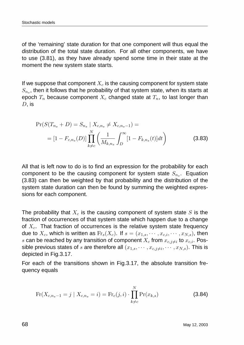
Stochastic models

of the ‘remaining’ state duration for that one component will thus equal thedistribution of the total state duration. For all other components, we haveto use (3.81), as they have already spend some time in their state at themoment the new system state starts.

If we suppose that component Xc is the causing component for system stateSns , then it follows that he probability of that system state, when its starts atepoch Tn because component Xc changed state at Tn, to last longer thanD, is

Pr(S(Tns + D) = Sns | Xc,ns 6= Xc,ns−1) =

= [1− Fc,ns(D)]N∏

k 6=c

(1

Mk,ns

∫ ∞

D[1− Fk,ns(t)]dt

)(3.83)

All that is left now to do is to find an expression for the probability for eachcomponent to be the causing component for system state Sns . Equation(3.83) can then be weighted by that probability and the distribution of thesystem state duration can then be found by summing the weighted expres-sions for each component.

The probability that Xc is the causing component of system state S is thefraction of occurrences of that system state which happen due to a changeof Xc. That fraction of occurrences is the relative system state frequencydue to Xc, which is written as Frs(Xc). If s = (x1,s, · · · , xc,i, · · · , xN,s), thens can be reached by any transition of component Xc from xc,j 6=i to xc,i. Pos-sible previous states of s are therefore all (x1,s, · · · , xc,j 6=i, · · · , xN,s). This isdepicted in Fig.3.17.

For each of the transitions shown in Fig.3.17, the absolute transition fre-quency equals

Fr(Xc,ns−1 = j | Xc,ns = i) = Frc(j, i) ·N∏

k 6=c

Pr(xk,s) (3.84)

68 May 12, 2003

Stochastic models

X 1 , . . . , X c = i , . . . , X N

X 1 , . . . , X c = 1 , . . . , X N

X 1 , . . . , X c = i - 1 , . . . , X N

X 1 , . . . , X c = i + 1 , . . . , X N

X 1 , . . . , X c = N c , . . . , X N

Figure 3.17: Transitions due to changing Xc

and the total transition frequency for any of these states to S thus equals

Fr(Xc,ns−1 6= i | Xc,ns = i) =Nc∑

j 6=i

Fr(Xc,ns−1 = j | Xc,ns = i)

= Frc,i

N∏

k 6=c

Pr(xk,s) (3.85)

For (3.85), it was used that Frc,i =∑Nc

j 6=i Frc(j, i), which expresses the factthat a component state frequency is the sum of the absolute transition fre-quencies into that state.

With (3.85), the probability that Xc causes S is now expressed as

Pr(Xc,ns−1 6= Xc,ns) =Fr(xc,s)

∏Nk 6=c Pr(xk,s)

∑Nc=1

(Fr(xc,s)

∏Nk 6=c Pr(xk,s)

) (3.86)

=Fr(xc,s)/Pr(xc,s))∑Nc=1 Fr(xc,s)/Pr(xc,s)

(3.87)

which results in

Pr(Xc,ns−1 6= Xc,ns) =1/Mc,s∑Nc=1 1/Mc,s

(3.88)

May 12, 2003 69

Stochastic models

For a Weibull-Markov system, (3.83) takes the form of

Pr(S(Tns + D) = Sns | Xc,ns 6= Xc,ns−1)

= e−�

Dηc,s

�βc,s N∏

k 6=c

1Mk,s

∫ ∞

ke−( t

ηk,s)βk,s

dt (3.89)

= e−�

Dηc,s

�βc,s C∏

k 6=c

ηk,s

Mk,sβk,s

[Γ

(1

βk,s

)− Γ

(1

βk,s, (

D

ηk,s)βk,s

)](3.90)

where Γ(x, y) denotes the incomplete gamma function for x from 0 to y.

The combination of (3.88) and (3.90) leads to the following expression forthe probability for the duration of system state S to last longer than D:

Pr(Tns+1 − Tns > D) =N∑

c=1

(Pr(Xc,ns−1 6= Xc,ns) · Pr(S(Tns + D) = Sns | Xc,ns 6= Xc,ns−1))

=∏N

c=1 γc,s(D)/Mc,s∑Nc=1 1/Mc,s

N∑

c=1

exp(−(D/ηc,s)

βc,s

)

γc,s(D)(3.91)

where

γc,i(D) =ηc,i

βc,i

[Γ

(1

βc,i

)− Γ

(1

βc,i,

(D

ηc,i

)βc,i)]

(3.92)

From equation 3.91 and 3.92, it is clear that the system state duration dis-tribution is independent of the previous system states in the steady statecase. The γc,i(D) function only depends on the component state durationdistribution parameters β and η. The γc,i(D) values for each component canthus be calculated prior to the actual reliability assessment.

3.5 Basic Power System Components

This chapter shows a possible implementation of a Weibull-Markov modelfor modeling stochastic power system components. The proposed methodsare introduced on the basis of a model for the synchronous generator.

70 May 12, 2003

Stochastic models

3.5.1 Defining a Weibull-Markov Model

The Weibull-Markov model is determined by the following set of parameters.

• N, the number of states

• {βi}, the set of form-factors, one for each state

• {ηi}, the set of characteristic times, one for each state

• P, the transition probability matrix

• Electrical parameters, which define the electrical model for the com-ponent for each state

It is however possible to enter the state duration parameters other than by βand η, as in many cases, these are unknown. Alternatively,

• {µi}, the mean state durations

• {σi}, the state duration variances

should be possible too.

Any two of the resulting possible state duration parameters, βi, ηi, µi, σi, willdetermine the other two. The following conversion formulas can be used:

May 12, 2003 71

Stochastic models

µ(β, η) = ηΓ1(β)

µ(β, σ) = Γ1(β)

√σ2

Γ2(β)

σ(β, η) =√

η2Γ2(β)

σ(β, µ) =µ√

Γ2(β)Γ1(β)

β(η, µ) = Γinv1

(µ

η

)

β(η, σ) = Γinv2

(µ

η

)

β(µ, σ) = Γinv3

(µ2

η2

)

η(β, µ) =µ

Γ1(β)

η(β, σ) =

√σ2

Γ2(β)

where

Γ1(β) = λΓ(1 +1β

)

Γ2(β) = Γ(1 +2β

)− Γ(1 +1β

)2

Γ3(β) =Γ1(β)2

Γ2(β)

The inversion of Γ1(β), Γ2(β) and Γ3(β) can be performed by newton meth-ods. De values for µ(η, σ), σ(η, µ) and η(µ, σ) can be calculated by firstcalculating the corresponding β.

The above set of conversion formulas enables an easy definition of a Weibull-Markov model. However, it is also possible to leave all form-factors {βi} to

72 May 12, 2003

Stochastic models

their default values of one, and enter the Weibull-Markov model as a ho-mogenous Markov model. Such would be needed if no other than homoge-nous model data is available. In stead of {βi}, {ηi} and P, the homogenousMarkov model requires the input of:

• {λij}, the matrix of state transition rates

This asks for the conversion of the state transition matrix to the transitionprobability matrix P. Such conversion can be done by using (3.36).

The back transformation from the state probability matrix to a state transi-tion matrix can be performed by using the calculated state duration meansand (3.38). This back transformation makes it possible to switch between‘homogenous input mode’ and ‘Weibull-Markov input mode’, which may beused to check the validity of the model or to check the correct transformationof a homogenous model into a more realistic Weibull-Markov model.

3.5.2 A Generator Model

The basic stochastic generator model is fairly primitive, as it only definesstates for the generator being available or not available. In many applica-tions, such a two-state model is sufficient. However, there are several rea-sons to include more states to account for partial outages of the generator.Such a partial outage is a condition in which the generator is still connectedto the net and is still producing power, but in which the maximum output islimited. Such a situation may occur when

• A run-of-the-river hydro turbine is reduced in capacity due to a low riverlevel.

• A large, multi-machine thermal power plant is reduced in capacity dueto the outage of one or more generator units.

• The available power is reduced due to the outage of a sub-component,such as a pulverizer, a fan, a feed water or cooling water pump, etc.

A state that models a partial outage is called a “derated state”. In orderto account for derated states, which number may differ from generator togenerator, it must be possible to freely define new states.

May 12, 2003 73

Stochastic models

The implementation of the dialog which is used to define a stochastic gener-ator is shown in Fig.3.18. This example shows a generator with two deratedstates which has been defined as a Weibull-Markov model after which thedialog was changed to the homogenous Markov mode. It therefore showsthe transition rate matrix and it would be possible to edit this matrix. Thismight be useful when stochastic data is available in several different formats,which are all to be translated into state transition rate models. The entry forthe “dependent state” in the figure is needed to calculate the remaining tran-sition probability, in order to make sure that the transition probabilities addup to one for each state.

Figure 3.18: The stochastic model for a synchronous generator

The electrical models for the different states of the synchronous generatoronly differ in the maximum available active power and in the number of avail-able machines. The latter is only of importance when the stochastic modelis used for a multi-machine power plant. The dialog for defining the electricalmodel is shown in Fig.3.19.Because the Weibull-Markov model allows for defining the shape of the stateduration distribution, the dialog has ‘graph’ page, which is shown in Fig.3.20.This page shows the duration distribution and a set of state parameters,

74 May 12, 2003

Stochastic models

Figure 3.19: Electrical parameters for the stochastic generator

such as the frequency and the MTBS (mean time between states). Thestate parameters are calculated from the entered model and are shown forreference and checking purposes. The shown graph page shows the distri-bution and state parameters for the ‘out of service’ state. The state probabil-ity informs the user that this generator is out of service for more than 10% oftime (942.1851 h/a), from which he may decide to check the stochastic dataused.

May 12, 2003 75

Stochastic models

Figure 3.20: State duration graph and state parameters

76 May 12, 2003

Chapter 4

Interruption CostsAssessment

4.1 Reliability Worth

Power system utilities try to maximize efficiency. They have to find the bestbalance between performance and cost. Regarding the reliability of sup-ply, they have to avoid too low a level of investments, because that will re-sult in excessive damage caused by supply interruptions, as well as over-investments.

The highest level of efficiency can only be reached by comparing the in-crease of performance with the required investment costs. The calculationof (expected) performance indicators in respect to supply reliability is thetask of the reliability assessment. This task can be divided into the calcu-lation of non-monetary interruption statistics and the calculation of reliabilityworth indices. Reliability worth assessment produces monetary indices, andis a relatively young discipline. The calculation of non-monetary interruptionstatistics is more established ([2], [3], [4], [12], [13], [16], [53]). This includesthe calculation of

• Interruption frequency.

• Mean interruption duration.

• Probability of not being supplied.

May 12, 2003 77

Interruption Costs Assessment

• Energy not supplied and mean interrupted power.

Two major problems arise if we use interruption statistics for investment jus-tification or for estimating the (relative) importance of the various parts of thesystem.

The first problem is the fact that we cannot directly compare the costs of in-creased reliability, which is in monetary units, with a non-monetary reliabilityperformance index. Non-monetary reliability indices can be used to estab-lish minimum system requirements or to rank different design alternatives.But they cannot be related to the investment costs.

The second problem is that the interruption statistics express the supplyreliability from the system’s point of view, i.e. they express the system per-formance within the context of the system alone. The supplied customersare only regarded as far as their electrical effects on the system. Customerswith identical electrical behaviour are treated equally. It is therefore difficult,if not impossible, to account for the effects of specific customer importanceor interruption damage functions in the calculated interruption statistics. Inother words, if the power consumption and the frequency and mean dura-tion of the power interruptions are identical for a hospital, for instance, and ashopping mall, then their calculated interruption statistics will also be iden-tical. It will not be possible to bias the non-monetary reliability performanceindices for the difference in importance of these two loads, even when thatimportance is known to be completely different.

One possible way to accommodate for customer importance is to use thecosts for the energy not supplied (money/kWh) and/or a cost per interruptedpower (money/kW) as an adjustable measure for interruption severity. Thiscan produce useful indices, but it is often insufficient for more detailed plan-ning or selection of alternatives. This linearization of the costs with the dura-tion of the interruption does not consider the fast increase with duration thatoccurs for individuals as well as for aggregated loads ([124]).

For investment justification or for comparing different design alternatives ona monetary basis or on the basis of interruption severity, we will have toconsider a more detailed interruption damage model.

78 May 12, 2003


4.2 Interruption Damage Functions

The assessed severity of the impact of a supply interruption, either plannedor unplanned, depends on many aspects. The major factors are the def-inition of the severity that is used, the type of interrupted customers, theduration of the interruption and the extent of the interrupted area.

The consequences of an interruption are quantified by a so-called “interrup-tion damage function”, which gives the consequences in monetary units asa function of the characteristics of the interruption.

The interruption damage function for a single point interruption and for multi-point interruptions, for example for large area interruptions, can be modeledin the same way. Single point damage models describe the interruptiondamage for a single load in the analyzed system. This load may model asingle household or a single asynchronous motor in an industrial process,but may also model a whole distribution network or a large factory. Thesingle point load will be interrupted as soon as the supply to the busbar towhich it is connected is interrupted. A multi-point damage model describesthe interruption damage for an area or a large industrial proces which aresupplied by more than one bus. The multi-point model has an additionaltrigger condition which defines the combinations of busbars that must beinterrupted in order for the damage function to apply.

In [46], the impacts of interruptions are classified as direct vs. indirect andeconomic vs. otherwise (social). Short interruptions in a small residentialarea will normally only cause direct damage, such as food spoilage or in-convenient building temperatures. More wide-spread interruptions with alonger duration will also cause indirect damage such as civil disobedience,breakdown of logistics chains, etc.The classification into direct and indirect costs, and into economic and non-economic costs, is not further discussed here. It is assumed that the impactsof interruptions can be quantified into cost functions, regardless of the natureof the impacts.

Interruption damage functions are often abstract estimations of the actualinterruption damage. Actual interruption damage may depend on

May 12, 2003 79


• The type of interrupted customers

• The duration of the interruption

• The situation in which the interruption occurs: day of week, time ofday, customer’s activities at the moment of interruption, etc.

As a different damage function can be assigned to each specific customer orcustomer mix, the dependency of the damage function itself can be furtherconfined to

• The duration of the interruption

• The moment of occurrence

When we consider the moment of occurrence, then we would have to de-fine damage functions for all recurrent situations for which the interruptiondamage is know to differ significantly. That could mean, for instance, thatwe have to define different damage functions for different times of the day,for different days of week, etc. Although it would be possible to create anduse arrays of damage functions for each customer, we would like to avoid itand use only one single damage function for each customer.

Specifying damage functions for specific intervals in time will only make adifference when there is also a significant difference in the probability of oc-curring for specific types of interruptions in these intervals. If interruptionsare equally likely to occur during periods of high interruption costs as dur-ing low cost periods, then we can average the damage costs by using therelative length of each period.

If we do not consider a time-dependent probability for the occurrence ofinterruptions, then we can thus use interruption damage models which areonly dependent on the duration of the interruption. This approximation isused in most studies. Considering the time-dependency of the interruptiondamage function only affects that results when also the time dependency ofthe failure rates are included in the calculations.

4.2.1 Sector Customer Damage Function

Data collected from customer surveys is used to create damage functionsfor certain classes or “sectors” of customers. These surveys give information

80 May 12, 2003


about the perceived interruption costs for each specific customer separately,and may contain information about the effect of the duration of the interrup-tion, the time of occurrence, the amount of interrupted power or energy, etc.

The “raw” data from the customer surveys has to be processed and trans-formed in order to create customer damage functions (CDF) which can alsobe projected upon customers which have not been surveyed.

The first step in the data transformation is performed by grouping all rawdamage functions according to some customer classification, for instancethe SIC (Standard Industrial Classification). Typical customer classes, orsectors, are “residential”, “industrial”, “commercial” , “government”, etc.

The raw damage functions are then normalized per group by using a specificcustomer parameter. This normalization parameter may be the measuredyearly peak demand, the yearly energy consumption, a combination of peakdemand and energy consumption, or other values. In some cases, normal-ization for shorter durations is done to annual peak demand, and to annualenergy consumption for longer durations ([19]).

When the normalization parameter is known for each raw damage function,then averaged damage functions can be calculated as

C(s, d) =N(s)∑

i=1

C(s, i, d)F (s, i)

(4.1)

where, for sector s and interruption duration d,

• C(s, d) is the averaged damage function,

• N(s) is the number of raw damage functions,

• C(s, i, d) is the raw damage function for customer i, and

• F (s, i) is the normalization factor for customer i

When the normalization factor is only known for the whole group of rawdamage functions, then an aggregating process can be used, for which

C ′(s,D) =∑N(s)

i=1 C(s, i, d)∑N(s)

i=1 F (s, i)(4.2)

May 12, 2003 81


SCDF 5000 kWh 8000 kWhduration $/kWh $ $

20 min. 0.0000235 0.12 0.19

1 hr 0.0000972 0.49 0.78

2 hrs 0.000273 1.37 2.18

4 hrs 0.000520 2.60 4.16

8 hrs 0.00129 6.45 10.32

1 day 0.00597 29.85 47.76

2 days 0.0138 69.00 110.40

Table 4.1: SCDF and scaled CDF for two customers

and C ′(s,D) ≤ C(s,D). Mixtures of averaging and aggregating can be usedwhen some, but not all, normalization factors are known.

The resulting averaged or aggregated damage function for a specific sectorof customers is called a Sector Customer Damage Function or SCDF.

4.2.2 Composite Customer Damage Function

The SCDF is not used in the actual reliability assessment itself. It is onlyused to create damage functions for single customers or for mixes of cus-tomers. The normalization process leads to SCDFs which have units like$/kWh or $/kW. In some cases these units have been misinterpreted ascosts per energy not supplied or per interrupted power.

If we want to create a customer damage function (CDF) for a single cus-tomer, then we need the SCDF for the sector and the normalization factorfor the customer. If yearly energy consumption has been used, then theSCDF will be in $/kWh. The CDF is then obtained by multiplying the SCDFwith the customer’s yearly consumption. This is illustrated in table 4.1, wherea SCDF is scaled to a customer of 5000 kWh and to a customer with 8000kWh.

82 May 12, 2003


If we need to create damage functions for a mix of customers, then we haveto create a composite customer damage function (CCDF). The CCDF is ba-sically the sum of the individual customer damage functions in the customermix. It can be constructed by taking the relative contribution of the variouscustomer sectors to the overall normalization factor. The weighted sum ofthe different SCDFs according to these relative contributions is then multi-plied by the overall factor.

4.3 Use of Damage Functions

The CDF and CCDF that result from the scaling of one or more SCDF’sdefine the damage for each interruption as a function of the interruption du-ration. This information is combined with the results of the FEA to calculateannual interruption costs for each load point and for the whole system.

4.3.1 Interruption Costs Calculations

The stochastic failure models are used to create specific system stateswhich are then analyzed. Such analysis may include load flow calculationsand topological analysis, but may also include power system protection al-gorithms, power restoration procedures and optimization methods, duringwhich the network is reconfigured and generation may be rescheduled.

The principle objective of the system state analysis is to express the abilityof the system to meet the load demands in preliminary performance indica-tors. These preliminary indicators are then used, at the end of the systemstate creation and analysis phase, to calculate overall performance indica-tors. The interruption costs indicators express the expected costs per yeardue to load interruptions. For each load point, the LPEIC (load point ex-pected interruption costs, $/a) indicator expresses the total expected costsper year due to the interruptions of the load point.

By drawing outcomes for the stochastic conditional state durations for eachcomponent, the duration of the current state and the number of the nextstate are determined. When the current state duration has passed, a transi-tion to the next state is made and new outcomes can be drawn to determine

May 12, 2003 83


the new duration and the following state. In this way, a possible history forthe component can be simulated in time. By performing a parallel simula-tion of all components in the system, the whole system can be simulated intime. This way of generating system states in a chronological order is called“Monte-Carlo simulation”.

Each time a new system state is reached during the Monte-Carlo simulation,it is analyzed for performance. Because the simulation of one single periodof, for instance, 5 years, would not make it possible to derive accurate overallperformance indicators, it is necessary to simulate and analyze the sameperiod a large number of times. The LPEIC is then calculated as

LPEIC =∑I

i=1 C(di)K · analyzed period

(4.3)

where C(di) is a single outcome of the interruption cost function C, for thesimulated duration di, I is the total number of interruptions of the consideredload point during the whole Monte-Carlo analysis, and K is the number oftimes the analyzed period (the length of which is expressed in years) wassimulated.

The Monte-Carlo simulation technique is very powerful because it allows forthe simulation of about any possible event in the system and it does not putany restriction on the stochastic component models. Its big disadvantage,however, is its high computational demand. The technique of system stateenumeration is therefore often used instead.

In a system state enumeration, all relevant system states are created andanalyzed one by one. In this case, no outcomes are drawn for the stochasticdurations, but the probabilities and frequencies of the system states arecalculated directly. An analytical reliability assessment by state enumerationproduces exact results for the performance indicators.

For the reliability costs indicators, such as the LPEIC, the state enumerationmethods, however, are problematic. In many textbooks and articles (e.g.[16],[66]), the following equation is used for calculating the LPEIC.

LPEIC =M∑

i=1

fi · C(di) (4.4)

84 May 12, 2003


where fi is the frequency of the ith system state that causes an interruptionof the load point and M is the number of different system states which leadto such interruption. This equation, however, is principally wrong, as it as-sumes that all interruptions caused by the ith system state are of durationdi. This is an assumption that can not be justified, as the durations of repairsor maintenance are stochastic.

The use of (4.4) is often defended by the assumption that power to an in-terrupted load will be restored by network reconfiguration, and not by re-pair. Network reconfiguration is often modeled by deterministic switchingdurations. Three arguments against the use of (4.4) in a state enumeratedreliability assessment can be formulated:

1. It is often unknown if power can be restored to all interrupted loads bynetwork reconfiguration alone in all cases. One objective of a reliabilityassessment may be to find cases where switched power restoration isnot possible.

2. The financial risk related to interruption costs cannot be assumed tobe determined by the majority of cases in which the restoration pro-cedures work as planned. Load interruption during unusual systemconditions may lead to unexpected high restoration durations. Suchmay happen in the case of failing protection devices, stuck breakers,unavailable (backup) transmission lines, peak load situations, etc.

3. Wide area power systems, or systems in rural areas, may lack therequired network reconfiguration options or may require the modelingof switching times as stochastic quantities.

4. Statistical data shows a considerable spread in interruption duration([30], [97], [43])

For a correct calculation of interruption costs or other reliability cost indi-cators, it is therefore necessary to assess the duration distribution of allinterruptions during a state enumerated reliability assessment. This is pos-sibly by using the Weibull-Markov model, as introduces in chapter 3. Thecalculation proceeds as follows:

• Expression (3.92) is evaluated for each stochastic model prior to theactual state enumeration

May 12, 2003 85


• Expression (3.91) is evaluated for each system state for which theprobability distribution of the duration is required.

This means that, if

• a CDF or CCDF has been defined as a vector {C(Tj)} for the interrup-tion durations {T1, · · · , TNc}

• the probability Pr(Tj−1 < Di < Tj) for the state duration Di can becalculated using (3.92).

then the expected interruption costs for the for the ith system state can becalculated as

E(Ci(d)) =Nc∑

j=1

Pr(Tj−1 < Di < Tj) · C(Tj) (4.5)

where Di is the stochastic system state duration.

With (4.5), the annual LPEIC can then be calculated as

LPEIC =M∑

i=1

fi · E(Ci(d)) (4.6)

where fi is the system state frequency.

The above method for calculating the LPEIC, i.e. using (3.92), (3.91) and(4.5) to evaluate (4.6) seems very complicated and time consuming. Indeed,when compared with (4.4), a slight increase in efforts cannot be denied.However, it has been found in practice that the evaluation of the LPEIC in thedescribed way increases the total computation time only very slightly. Whenthe proposed method is analyzed for required computational demands, it isclear why the computational demand is very moderate:

• Expression (3.92) is evaluated for each stochastic component sepa-rately, and only has to be analyzed once, prior to the reliability analy-sis. The results can be stored with the stochastic model model. Thecomputational demand is thus very low or zero.

86 May 12, 2003


• Expression (3.91) is evaluated for each analyzed system state. Thecomputation demand is very small, as it only requires the multiplicationor addition of a few known factors.

• The evaluation of (4.5) and (4.6) is very fast, and linear with the numberof load points.

The low computational demands and the very simple expressions that are tobe evaluated, of which the most complex can be evaluated a-priori, make theproposed method of calculating the LPEIC elegant, transparent and practi-cal.

4.4 Effects of the Interruption Duration Distribution

The ability to calculate reliability worth on the basis of the probability distri-bution of the interruption duration is only of practical use when the shape ofthis distribution is relevant. It is easy to define customer damage functionsfor which the LPEIC would become highly dependent on the interruption du-ration distributions. It is also clear that the use of linear damage functions,results in a LPEIC that is completely independent of the interruption dura-tion distribution. It is therefore required to evaluated the importance of theinterruption duration distributions on the basis of realistic damage functions.

A number of customer surveys have been undertaken in various countriesover the whole world in the last decades. The Cigré Task Force 38.06.01discusses the use of interruption costs functions in power system analysis,and has published an overview of surveyed data in ([46]).

One of the conclusions of the task force is that “The actual event basedapproach can provide ECOST values which are significantly different fromthose obtained by the average event (analytical) method if the applied CDFare highly non-linear.” ([46]). Although the report continues by saying that“In most cases, however, either technique will provide acceptable results.”,it does not indicate in which cases average event methods give acceptableresults and in which cases they produce unacceptable errors.

In order to quantify the errors in calculated LPEIC values, the publishedcustomer damage functions in [46] where analyzed for their sensitivity to

May 12, 2003 87


the probability distribution of the interruption duration. This analysis wasperformed in the following way:

• A Weibull distribution of the interruption duration was presumed.

• The mean costs per interruption was evaluated for various values ofthe β-shape factor of the duration distribution, and for four differentmean durations. A linear interpolation of the customer damage wasused for interruption durations in between the discrete values of thedamage function.

• The resulting four functions, each of which gives the mean costs asfunction of the β factor for a certain mean duration, are divided by themean costs for a unity shape factor, i.e. for β = 1.

• The value of the relative mean costs was interpreted as an “error func-tion” which indicates the possible error that could result when the dam-age function is used in a reliability calculation in which the durationdistribution is either not considered or modeled incorrectly.

The Weibull distribution is chosen as a model for the interruption durationdistribution because measurements indicate that interruption durations areoften more or less Weibull distributed ([128]). Another reason is that theWeibull distribution also covers the exponential distribution, and a compari-son with results from a homogenous Markov model is therefore possible.

The SCDF for commercial customers in Canada, according to [46], is usedhere as example, to describe the above analysis method in more detail. TheSCDF is shown in table 4.2, in 1999 US$. The mean interruption costs for aWeibull distributed interruption duration, was calculated as

EC(β, µ) = EC(β, η(µ)) =∫ ∞

0C(τ) · β

ηβτβ−1 exp

[−

(τ

η

)β]

dτ (4.7)

where η = η(µ) is the scale factor of the Weibull distribution which corre-sponds to a mean of µ and where C(τ) is the SCDF, in this example accord-ing to table 4.2, which was linearly interpolated.

The function EC(β, µ = M) describes the dependency of the interruptioncosts to the β form factor, for a fixed mean duration M . Each of these

88 May 12, 2003


$/kW

2 sec. 0.232

1 min. 1.63

20 min. 4.83

1 hr 13.0

2 hrs 27.3

4 hrs 65.7

8 hrs 106

1 day 127

Table 4.2: SCDF for “Canada, Commercial, $/kW”

functions is subsequently divided by EC(1.0,M), which results in an “errorfunction” which describes the deviations for various β-factors independentlyof the used SCDF. These error functions have been calculated for a meanduration (µ) of 10 minutes, 30 minutes, 1 hour and 4 hours. The results forthe example SCDF are depicted in Fig.4.1.The error function for a mean duration of 4 hours in Fig.4.1 shows valuesin excess of 20% for β > 2.5. This means, for the example SCDF, that notregarding the effects of the interruption duration distribution correctly couldlead to errors of 20% or more in the calculated LPEIC index.

The analysis described above was carried out on all damage functions pub-lished in ([46]). The largest deviations which were found are listed in table4.3. The results of all analyzed damage functions are shown in appendix A.

Note that these results are based on “average customers” and interruptiondurations with a Weibull probability distribution. For individual customersand other distributions, the results may even be larger. However, no datawas available to substantiate this.

From the analysis of the damage functions, it is clear that the dependencyof the interruption costs to the interruption duration and the probability distri-

May 12, 2003 89


SCDF largest deviation

Saudi Arabia Residential 66 %

Saudi Arabia Industrial 45 %

Saudi Arabia Commercial 39 %

Norway Agriculture 33 %

Greece Companies+organisations 27 %

Australia Commercial 25 %

Canada Commercial 25 %

Nepal Commercial 25 %

Greece Commercial total 23 %

Denmark Household 22 %

Sweden Commercial 20 %

Australia Major User 19 %

Greece Business 19 %

Sweden Agriculture 19 %

Australia Residential 18 %

Sweden Residential 18 %

Great Britain Industrial 16 %

Greece Industrial 16 %

Table 4.3: Largest deviations for analyzed international CDF.

90 May 12, 2003


0 1 2 3 4 50.6

0.7

0.8

0.9

1

1.1

1.2

1.3

1.4Canada Commercial $/kW

shape factor

10 min. 30 min. 1 hr. 4 hrs.

Figure 4.1: PDF dependency for “Canada, Commercial, $/kW”

bution of that duration cannot always be ignored. It would be allowed to ig-nore these factors when damage function are used which are (almost) linearfunctions of the interruption durations. The use of homogenous calculationmethods will produce correct results for such functions. In all other cases,the use of homogenous methods bears the risk of producing reliability worthindices with large errors.

May 12, 2003 91

Chapter 5

Example

An example is shown here for an 11kV distribution system. This system is amodification of the test system described in [6], which was based on a realUK system. This system is chosen here because of its size and complexity.

5.1 Description of the Test System

A single line diagram of the test system is displayed in Fig.5.1. Some pa-rameters describing the size of the test system are given in table 5.1.The test system is a radially operated distribution network, in which all loadscan be fed from two sides.

Test System Parameters

Number of Nodes 85

Number of Lines 30

Number of transformers 13

Number of Loads 56

Total Demand 52.08 MW

Table 5.1: Size of the test system.

92 May 12, 2003

Example

C09b C09c C09d

C08

a C

08b

C10

c C

10a

C11

c C

11a

C11

b

T10

11b

C23

a C

12c

C12

b C

12a

C15

c C

15a

C15

b

ES2

T10

11a

C06b

C04b

T1201b

T1201a

T09

11

C09

a

C10

b

C14b C14c C14a

Cable02b

Cable02a

T0305

T0405

C02a

Linet0601

T06

08

T07

08

Line

0907

T0102a

T0102b

ES

7

Line0113b T01

13a

Line0113a

T01

13b

C17b C17c C17a

C16c C16b

ES

8

C16a

ES

5 E

S3

Cab0113b

Cab0113a

ES

4

Cable06t06

C20b C20a

C13

b C

13a

C05

a C

05c

C05

b

C06c C06a

C04a C04c

C22

a C

22b

C03c

C02d

Cable0109

C03a

C02b

C03b

C02c

C07

c C

07a

C07

b

C21c C21a C21b

Cable0110

S13

c S

13b

S13

a

S06d S06c S06b S06a

S23b

S23

a

S09a S09b S09c S09d

S08

d S

08c

S08

e S

08b

S08a

S03d S03c S03b S03a

S21c

S21

d

S21

a

S21b

S07d

S07

c S

07b

S07

a

S04b S04a S04d S04c

S22

b S

22a

S22

d S

22c

S05

b S

05a

S05

d S

05c

S12

c S

12d

S12

b S

12a

S11d

S11

c S

11b

S11

a

S10

e S

10d

S10

b S

10a

S10

c

S02d S02c S02b S02f S02e

S02

a

S20d S20c S20b S20a

S14c S14b

S14

d

S14a

S15

d S

15c

S15

b S

15a S17b S17c S17d S17a

S16d S16c S16b S16a

B05

B08

B02

B12

B11

B13

B01

B04

B07

B09

Figure 5.1: The distribution test system

May 12, 2003 93

Example

$ $/kW $/kWh

2 sec. 122 0.232 0.00105

1 min. 148 1.63 0.000986

20 min. 347 4.83 0.00235

1 hr 1023 13.0 0.00700

2 hrs 1806 27.3 0.0123

4 hrs 3767 65.7 0.0278

8 hrs 6756 106 0.0477

1 day 14831 127 0.0987

Table 5.2: Interruption Cost Function

The peak load demands for the load points are listed in table 5.3. Each loadpoint was given a fixed number of customers,which is also listed in table5.3. All loads have the same interruption cost function, according to table5.2. This cost function is the one for the commercial customers in Canada,according to [46]. The SCDF per kW peak demand was used by all loadsand was automatically scaled to the kW peak demand (according to table5.3) during the reliability assessment.

The failure data used for lines, cables, transformers and busbars is listedin tables 5.4 and 5.5. Common mode failure models were defined for thecables which are encircled in the single line diagram. The data for thesecommon failures is shown in table 5.4.

94 May 12, 2003

Example

Name MW MVAr Cust. Name MW MVAr Cust.

C02a 0.50 0.020 100 C11a 0.40 0.081 80C02b 0.52 0.020 104 C11b 0.30 0.061 60C02c 0.40 0.020 80 C11c 0.40 0.081 80C02d 0.90 0.183 180 C12a 1.50 0.305 300C03a 0.54 0.020 108 C12b 1.20 0.244 240C03b 0.62 0.020 124 C12c 1.20 0.244 240C03c 1.10 0.223 220 C13a 2.20 0.447 440C04a 0.90 0.183 180 C13b 2.20 0.447 440C04b 0.40 0.081 80 C14a 0.10 0.020 20C04c 1.60 0.325 320 C14b 0.10 0.020 20C05a 1.00 0.203 200 C14c 1.70 0.345 340C05b 1.40 0.284 280 C15a 1.80 0.366 360C05c 2.30 0.020 460 C15b 0.70 0.142 140C06a 1.00 0.203 200 C15c 1.20 0.244 240C06b 1.40 0.284 280 C16a 0.10 0.020 20C06c 1.90 0.386 380 C16b 0.10 0.020 20C07a 1.20 0.244 240 C16c 0.80 0.162 160C07b 0.90 0.183 180 C17a 0.10 0.020 20C07c 2.10 0.426 420 C17b 0.10 0.020 20C08a 0.74 0.150 148 C17c 1.40 0.284 280C08b 0.90 0.183 180 C20a 0.10 0.020 20C09a 0.74 0.150 148 C20b 1.40 0.284 280C09b 0.74 0.150 148 C21a 0.10 0.020 20C09c 0.74 0.150 148 C21b 0.30 0.061 60C09d 0.74 0.150 148 C21c 0.50 0.102 100C10a 0.90 0.183 180 C22a 1.40 0.284 280C10b 0.90 0.183 180 C22b 1.70 0.345 340C10c 0.40 0.081 80 C23a 1.50 0.305 300

Table 5.3: Load Data

May 12, 2003 95

Example

Name Failure RepairFrequency Mean β

1/a hCables 0113a + 0113b 0.01 300 2.0Cables 02a + 02b 0.03 300 2.0Lines 0109 + 0110 0.05 300 2.0Lines 0113a + 0113b 0.05 300 2.011kV Cables 3.2/100km 33.5 3.533kV Cables 3.2/100km 33.5 3.533kV Overhead Lines 2.5/100km 212 3.5Transformers 0.02 343 1.5

Table 5.4: Common mode and branch failure data

BusBar Failure Field Failure RepairName Freq. Freq. Mean β

1/a 1/a h11kV Bar 0.002 0.005 14 2.533kV Bar 0.0025 0.015 24 2.5

Table 5.5: Busbar failure data

96 May 12, 2003

Example

System IndicesCustomer Avg. Interruption Frequency Index CAIFI 0.128 1/CaCustomer Avg. Interruption Duration Index CAIDI 5.92 hAvg. Service Availability Index ASAI 99.9913 %Energy Not Supplied ENS 39.6 MWh/aAvg. Customer Curtailment Index ACCI 3.80 kWh/CaExpected Interruption Cost EIC 259 k$/aInterrupted Energy Assessment Rate IEAR 6.55 $/kWh

Table 5.6: Overall system reliability indices

A reliability assessment was made for the whole system in the single linediagram. Overlapping failures were not considered. The reliability assess-ment produced overall system indices as well as indices for all individualload points in the system. Interruption costs were also calculated for everyindividual load point and for the overall system.

The first calculation was made using the β-factors for the Weibull distribu-tions of the repair durations, as shown in the tables 5.4 and 5.5. The resultsfor some system indices are shown in table 5.6. In table 5.7, the resultsfor the 20 load points with the highest interrupted customer-frequency areshown.

The 10 highest and 10 lowest values for the ACIF and the ACIT are shownin the bar-graphs of Fig.5.2 and Fig.5.3.

May 12, 2003 97

Example

Load Point IndicesName LPIF LPIT AID LPENS LPEIC ACIF ACIT

C/a Ch/a h MWh/a k$/a 1/a h/aC14c 70.3 239.0 3.40 1.19 9.49 0.207 0.703C20b 67.6 166.6 2.46 0.83 8.20 0.242 0.595C12a 64.1 293.2 4.58 1.47 11.69 0.214 0.977C07a 52.2 184.7 3.54 0.92 5.96 0.218 0.770C15c 52.2 251.8 4.82 1.26 12.76 0.218 1.049C12b 51.2 234.5 4.58 1.17 9.35 0.214 0.977C23a 47.4 272.0 5.74 1.36 7.63 0.158 0.907C07c 42.0 247.2 5.89 1.24 7.13 0.100 0.589C07b 39.2 143.1 3.65 0.72 4.65 0.218 0.795C06c 38.0 306.9 8.08 1.53 7.55 0.100 0.808C12c 37.9 139.6 3.68 0.70 6.06 0.158 0.582C06b 37.8 221.3 5.86 1.11 6.72 0.135 0.791C22a 37.8 157.1 4.16 0.79 4.48 0.135 0.561C13a 33.9 471.4 13.91 2.36 13.36 0.077 1.071C13b 33.9 471.4 13.91 2.36 13.36 0.077 1.071C04c 32.0 176.8 5.53 0.88 4.85 0.100 0.553C09a 30.5 149.5 4.90 0.75 5.48 0.206 1.010C09b 30.5 108.9 3.57 0.54 4.07 0.206 0.736C09c 30.5 103.0 3.37 0.51 3.65 0.206 0.696C09d 30.5 97.1 3.18 0.49 3.24 0.206 0.656

Table 5.7: Load point reliability indices

98 May 12, 2003

Example

C15

b C

17a

C3a

C

3b

C13

a C

13b

C15

c C

9a

C8a

C

8b

C10

b C

2d

C16

a C

16b

C17

c C

14b

C22

b C

5b

C14

a C

4b

1.25

1.00

0.75

0.50

0.25

0.00

Average Customer Interruption Time in h/a

Figure 5.2: Average Customer Interruption Time

C20

b C

15b

C15

c C

7b

C7a

C

12a

C12

b C

14c

C9a

C

9b

C17

a C

17b

C5c

C

2d

C22

b C

16a

C14

b C

14a

C21

a C

20a

0.25

0.20

0.15

0.10

0.05

0.00

Average Customer Interruption Frequency in 1/a

Figure 5.3: Average Customer Interruption Frequency

May 12, 2003 99

Example

5.2 Markov vs. Weibull-Markov Models

After the first “Weibull-Markov” calculation all β-factors in the failure modelswere set to unity. This results in a homogenous Markov system. A reliabil-ity calculation for the homogenous system was then started without furtherchanges. The results for all non-monetary indices were the same, as ex-pected. Only the values for the interruption costs where different. Fig.5.4shows the bar graphs for the LPEIC index, for both the Weibull-Markov cal-culation and the homogenous calculation.

Load Point Expected Interruption Costs in k$/a

C13

a C

13b

C15

c C

12a

C15

a C

14c

C12

b C

05c

C15

b C

20b

C11

a C

04b

C17

a C

21a

C17

b C

16b

C16

a C

20a

C14

b C

14a

15.0

12.0

9.0

6.0

3.0

0.0

Homogenous Markov Weibul-Markov

Figure 5.4: Load Point Expected Interruption Costs

The difference between the Markov and the Weibull-Markov calculation iswell over 16 % for the higher values of the LPEIC, and up to 18 % for allloads. These differences are calculated as relative to the Weibull-Markovresults and can thus be interpreted as the relative error of the homogenousresults.

The differences of 16 % and more are remarkable because power to inter-rupted loads in the test system can almost always be restored by switching

100 May 12, 2003

Example

actions. Interruptions which are restored by switching have short durationand therefore cause low costs. Repaired interruptions, on the other hand,have long duration and therefore cause higher costs. Switching actions weremodeled with deterministic durations. This means that the interruption dura-tion could be different for different failures, but had always the same durationfor the same failure. The duration of switched restorations is therefore notaffected by a change in a β parameter of a stochastic mode, as no stochasticmode is used for determining the duration of switched restorations.However, from the results it is clear that, although the repaired restorationsare less frequent than the switched restorations, they nevertheless have asignificant effect on the overall interruption costs due to the higher cost perinterruption. Otherwise there would not be a difference between the ho-mogenous and the Weibull-Markov results.

A second comparison was made in which a ‘single penalty’ interruption costsfunction was used. This costs function was zero for all interruptions shorterthan 8 hours and equaled 50$ for interruptions with a duration longer than8 hours. Again, a Weibull-Markov calculation was made, with the original β-factors, and a homogenous Markov calculation, with all β-factors set to unityagain. The resulting LPEIC values for the Weibull-Markov and the Markovcalculation are shown in Fig.5.5. The difference between the Markov andthe Weibull-Markov results are now exceeding 30 %.

5.3 Monte Carlo Simulation vs. State Enumeration

To investigate the correctness of the interruption costs calculations by an-alytic state enumeration methods, using Weibull-Markov models, compar-isons with Monte Carlo simulations were made.

The Monte-Carlo simulation produces averaged values, but also confidencelimits. A 95% confidence level was used. The results of the comparison areshown in Fig.5.6.

The Fig.5.6 shows that the results of the state enumeration method arewithin the 95 % confidence intervals as calculated by the Monte Carlo simu-lation.

May 12, 2003 101

Example

C13

a C

13b

C05

c C

06c

C06

b C

12a

C07

c C

23a

C15

a C

12b

C11

a C

04b

C17

a C

21a

C20

a C

16a

C17

b C

16b

C14

a C

14b

5.0

4.0

3.0

2.0

1.0

0.0

Load Point Expected Interruption Costs in k$/a

Homogenous Markov Weibul-Markov

Figure 5.5: LPEIC for ‘single penalty’ interruption costs

C13

a C

13b

C05

c C

06c

C06

b C

12a

C07

c C

23a

C15

a C

12b

C08

b C

06a

C04

c C

03c

C22

a C

08a

C05

a C

04a

C07

a C

15c

6.25

5.00

3.75

2.50

1.25

0.00

lower confidence level

upper confidence level Monte Carlo simulation State enumeration

LPEIC : Monte Carlo Simulation vs. State Enumeration

Figure 5.6: LPEIC, comparison

102 May 12, 2003

Chapter 6

Conclusions

The commonly used homogenous Markov model can be extended to includeWeibull-distributed state durations. The so-called t’t’Weibull-Markov” compo-nent is a semi-Markov model of a power-system component. Instead of anexponential distribution, a Weibull distribution is used for the state duration.

A system consisting of Weibull-Markov components is referred to as a Weibull-Markov system. A Weibull-Markov system does not longer obey the Markovproperty. It is therefore not a semi-Markov model. It is shown in this thesisthat it is possible to obtain an analytical expression for the state-durationdistribution for each of the states of the Weibull-Markov system.

The Weibull-Markov stochastic model as introduced in this thesis is “upwardcompatible” with the homogenous Markov model. All existing failure datacan also be used for the Weibull-Markov model. The Weibull-Markov modelexpands the homogenous Markov model by enabling the assessment of theprobability distribution for the system state durations.

The Weibull-Markov model can be used to obtain more correct results for theprobability distribution of interruptions of the power supply. This distributionis especially important when estimating the worth of reliability.

The expected annual interruption costs are normally calculated on the basisof customer damage functions. These damage functions define the costs ofan interruption as a function of the interruption duration.

May 12, 2003 103

Conclusions

The mathematically correct way of calculating the expected interruption costis by multiplying the damage function by the probability density function ofthe interruption duration. Calculation methods, however, which exclusivelyuse the homogenous Markov model, are not able to assess this densityfunction. It is shows in this thesis that, when homogenous Markov modelsare used despite this inability, errors of 40 % and more in the calculatedexpected interruption costs may result.

It has been shown that the results of an analytical state enumeration methodwhich uses the Weibull-Markov model, are comparable with the results ofa Monte-Carlo simulation. The computational demands for the proposedcalculation methods are comparable with the demands for the homogenousMarkov methods.

It should also be noted that an analytical method allows more conclusionsto be drawn from the results than a Monte-Carlo simulation.

Summarizing, the proposed methods for calculating expected yearly inter-ruption costs, based on the Weibull-Markov model,

• give more accurate results for the expected yearly interruption costs

• offer more flexibility in the use of customer damage functions

• do not effectively increase the computational demand

• are simple to implement, and easy to use.

Future work on power-system reliability should include a thorough investiga-tion of the various duration distributions needed for the component models.Interesting examples are the modeling of life-time distributions in combina-tion with maintenance for the time-to-failure, and the modeling of componentrepair-time distributions in combination with switching actions for the time-to-restoration. plement, and easy to use.

104 May 12, 2003

Appendix A

Analyzed International CDF

This appendix gives customer damage functions for a range of customersectors in various countries. All damage functions are based on the datagiven in [46].

All interruption costs functions shown in this sections are given in 1999 US$.

A.1 Australia

The costs data for Australia was obtained in studies conducted in 1996 and1997 by the Reliability Research Group at the CEPE, Monash University.

May 12, 2003 105


Residential Commercial Agricultural

$ $/kWh $ $/kWh $ $/kWh

2 sec. 281 0.00188

1 min. 511 0.00163 17.3 0.00456

20 min. 0.162 0.0000235 1156 0.00376 61.0 0.00658

1 hr 0.591 0.0000972 1277 0.00654 126 0.00915

2 hrs 1.60 0.000273 2908 0.00527 184 0.0111

4 hrs 3.30 0.000520 5178 0.00939 433 0.0336

8 hrs 8.04 0.00129 6789 0.0302 885 0.0549

1 day 35.2 0.00597 10468 0.0410 1926 0.151

2 days 81.5 0.0138

Table A.1: Australia, SCDF for “Residential”, “Commercial” and “Agricultural”

Industrial Major User Ind. + Major

$ $/kWh $ $/kWh $ $/kWh

2 sec. 1187 0.000331 4902 0.000175 2383 0.000202

1 min. 1827 0.00115 6114 0.000175 3135 0.000341

20 min. 2176 0.00150 7517 0.000373 3425 0.000593

1 hr 3579 0.00207 15169 0.00121 6944 0.00133

2 hrs 4092 0.00328 14580 0.000709 7089 0.00114

4 hrs 8019 0.00745 22344 0.00133 12269 0.00236

8 hrs 15223 0.0144 57464 0.00439 26286 0.00610

1 day 19974 0.0155 94709 0.00822 40437 0.00933

Table A.2: Australia, SCDF for “Industrial”, “Major User” and “Industrial +Major User”

106 May 12, 2003


0 1 2 3 4 50.6

0.7

0.8

0.9

1

1.1

1.2

1.3

1.4Australia Residential $

shape factor

10 min. 30 min. 1 hr. 4 hrs.

0 1 2 3 4 50.6

0.7

0.8

0.9

1

1.1

1.2

1.3

1.4Australia Commercial $

shape factor

10 min. 30 min. 1 hr. 4 hrs.

0 1 2 3 4 50.6

0.7

0.8

0.9

1

1.1

1.2

1.3

1.4Australia Residential $/kWh

shape factor

10 min. 30 min. 1 hr. 4 hrs.

0 1 2 3 4 50.6

0.7

0.8

0.9

1

1.1

1.2

1.3

1.4Australia Commercial $/kWh

shape factor

10 min. 30 min. 1 hr. 4 hrs.

0 1 2 3 4 50.6

0.7

0.8

0.9

1

1.1

1.2

1.3

1.4Australia Agricultural $

shape factor

10 min. 30 min. 1 hr. 4 hrs.

0 1 2 3 4 50.6

0.7

0.8

0.9

1

1.1

1.2

1.3

1.4Australia Industrial $

shape factor

10 min. 30 min. 1 hr. 4 hrs.

May 12, 2003 107


0 1 2 3 4 50.6

0.7

0.8

0.9

1

1.1

1.2

1.3

1.4Australia Agricultural $/kWh

shape factor

10 min. 30 min. 1 hr. 4 hrs.

0 1 2 3 4 50.6

0.7

0.8

0.9

1

1.1

1.2

1.3

1.4Australia Industrial $/kWh

shape factor

10 min. 30 min. 1 hr. 4 hrs.

0 1 2 3 4 50.6

0.7

0.8

0.9

1

1.1

1.2

1.3

1.4Australia Major User $

shape factor

10 min. 30 min. 1 hr. 4 hrs.

0 1 2 3 4 50.6

0.7

0.8

0.9

1

1.1

1.2

1.3

1.4Australia Industrial+Major User $

shape factor

10 min. 30 min. 1 hr. 4 hrs.

0 1 2 3 4 50.6

0.7

0.8

0.9

1

1.1

1.2

1.3

1.4Australia Major User $/kWh

shape factor

10 min. 30 min. 1 hr. 4 hrs.

0 1 2 3 4 50.6

0.7

0.8

0.9

1

1.1

1.2

1.3

1.4Australia Industrial+Major User $/kWh

shape factor

10 min. 30 min. 1 hr. 4 hrs.

108 May 12, 2003


A.2 Canada

The university of Saskatchewan conducted various customer damage sur-vey in Canada, with some regularity from the 1970’s onwards. Here pub-lished data is taken from the 1987 survey into agricultural interruption costs,the 1991 surveys into residential, commercial and industrial customers, andthe 1995 study of interruption costs for government, institute and office build-ings (GIO).

Agricultural Commercial

$ $/kW $/kWh $ $/kW $/kWh

2 sec. 122 0.232 0.00105

1 min. 148 1.63 0.000986

20 min. 1.13 0.0487 0.0000229 347 4.83 0.00235

1 hr 5.71 0.243 0.000115 1023 13.0 0.00700

2 hrs 1806 27.3 0.0123

4 hrs 47.2 2.02 0.000966 3767 65.7 0.0278

8 hrs 133 5.64 0.00270 6756 106 0.0477

1 day 14831 127 0.0987

Table A.3: Canada, SCDF for “Agricultural” and “Commercial”

0 1 2 3 4 50.6

0.7

0.8

0.9

1

1.1

1.2

1.3

1.4Canada Agricultural $

shape factor

10 min. 30 min. 1 hr. 4 hrs.

0 1 2 3 4 50.6

0.7

0.8

0.9

1

1.1

1.2

1.3

1.4Canada Commercial $

shape factor

10 min. 30 min. 1 hr. 4 hrs.

May 12, 2003 109


Gov., Inst., Off. Industrial


2 sec. 108 1.21 0.000258 907 0.782 0.00790

1 min. 1032 1.87 0.00821

20 min. 344 2.39 0.000803 1489 2.67 0.00868

1 hr 782 5.30 0.00197 2876 5.65 0.0109

2 hrs 4161 10.0 0.0128

4 hrs 2757 15.6 0.00686 7352 20.6 0.0195

8 hrs 12825 38.1 0.0364

1 day 21381 60.7 0.0485

Table A.4: Canada, SCDF for “Government, Institutes, Office Buildings” and“Industrial”

Residential

$ $/kW $/kWh

20 min. 0.190 0.0241 0.0000121

1 hr 1.10 0.141 0.0000701

4 hrs 12.1 1.57 0.000779

8 hrs 25.8 3.46 0.00172

1 day 117 15.8 0.00784

Table A.5: Canada, SCDF for “Residential”

110 May 12, 2003


0 1 2 3 4 50.6

0.7

0.8

0.9

1

1.1

1.2

1.3

1.4Canada Agricultural $/kW

shape factor

10 min. 30 min. 1 hr. 4 hrs.

0 1 2 3 4 50.6

0.7

0.8

0.9

1

1.1

1.2

1.3

1.4Canada Commercial $/kW

shape factor

10 min. 30 min. 1 hr. 4 hrs.

0 1 2 3 4 50.6

0.7

0.8

0.9

1

1.1

1.2

1.3

1.4Canada Agricultural $/kWh

shape factor

10 min. 30 min. 1 hr. 4 hrs.

0 1 2 3 4 50.6

0.7

0.8

0.9

1

1.1

1.2

1.3

1.4Canada Commercial $/kWh

shape factor

10 min. 30 min. 1 hr. 4 hrs.

0 1 2 3 4 50.6

0.7

0.8

0.9

1

1.1

1.2

1.3

1.4Canada Gov.−Int.−Office $

shape factor

10 min. 30 min. 1 hr. 4 hrs.

0 1 2 3 4 50.6

0.7

0.8

0.9

1

1.1

1.2

1.3

1.4Canada Industrial $

shape factor

10 min. 30 min. 1 hr. 4 hrs.

May 12, 2003 111


0 1 2 3 4 50.6

0.7

0.8

0.9

1

1.1

1.2

1.3

1.4Canada Gov.−Int.−Office $/kW

shape factor

10 min. 30 min. 1 hr. 4 hrs.

0 1 2 3 4 50.6

0.7

0.8

0.9

1

1.1

1.2

1.3

1.4Canada Industrial $/kW

shape factor

10 min. 30 min. 1 hr. 4 hrs.

0 1 2 3 4 50.6

0.7

0.8

0.9

1

1.1

1.2

1.3

1.4Canada Gov.−Int.−Office $/kWh

shape factor

10 min. 30 min. 1 hr. 4 hrs.

0 1 2 3 4 50.6

0.7

0.8

0.9

1

1.1

1.2

1.3

1.4Canada Industrial $/kWh

shape factor

10 min. 30 min. 1 hr. 4 hrs.

0 1 2 3 4 50.6

0.7

0.8

0.9

1

1.1

1.2

1.3

1.4Canada Residential $

shape factor

10 min. 30 min. 1 hr. 4 hrs.

0 1 2 3 4 50.6

0.7

0.8

0.9

1

1.1

1.2

1.3

1.4Canada Residential $/kW

shape factor

10 min. 30 min. 1 hr. 4 hrs.

112 May 12, 2003


0 1 2 3 4 50.6

0.7

0.8

0.9

1

1.1

1.2

1.3

1.4Canada Residential $/kWh

shape factor

10 min. 30 min. 1 hr. 4 hrs.

A.3 Denmark

The damage functions which have been analyzed are from the 1994 inves-tigation, which was initiated by the Nordic Council of Ministers. The showncosts are the interruptions losses as estimated by the customers.

Agri. Household Industry Public Ret. + Serv.

$/kW $/kW $/kW $/kW $/kW

1 sec. 1.17 0.339 0.508

1 min. 3.28 0.339 0.555

15 min 9.57 2.99 1.40

1 hr 55.0 5.42 18.2 7.44 7.04

4 hrs 16.4 35.3 24.7 22.6

8 hrs 226 50.4 58.9 47.5 46.6

Table A.6: Denmark, SCDF for “Agriculture-summer”, “Household”, “Indus-try”, “Public sector” and “Retail+Service”

May 12, 2003 113


0 1 2 3 4 50.6

0.7

0.8

0.9

1

1.1

1.2

1.3

1.4Denmark Agriculture summer $/kW

shape factor

10 min. 30 min. 1 hr. 4 hrs.

0 1 2 3 4 50.6

0.7

0.8

0.9

1

1.1

1.2

1.3

1.4Denmark Household $/kW

shape factor

10 min. 30 min. 1 hr. 4 hrs.

0 1 2 3 4 50.6

0.7

0.8

0.9

1

1.1

1.2

1.3

1.4Denmark Industry $/kW

shape factor

10 min. 30 min. 1 hr. 4 hrs.

0 1 2 3 4 50.6

0.7

0.8

0.9

1

1.1

1.2

1.3

1.4Denmark Public sector $/kW

shape factor

10 min. 30 min. 1 hr. 4 hrs.

0 1 2 3 4 50.6

0.7

0.8

0.9

1

1.1

1.2

1.3

1.4Denmark Retail+Service $/kW

shape factor

10 min. 30 min. 1 hr. 4 hrs.

114 May 12, 2003


A.4 Great Britain

The analyzed costs are from the 1993 survey, conducted by the ManchesterCentre for Electrical Energy at UMIST (University of Manchester Institute ofScience and Technology). The shown costs are the interruption costs asperceived by the customers.

Commercial Industrial


1 sec. 18.2 1.57 730 1905 9.76 4794

1 min. 18.6 1.62 762 2381 10.3 4968

20 min. 78.0 6.17 2603 4603 22.7 10032

1 hr 168 16.9 7794 6825 40.1 18952

4 hrs 548 62.0 28778 12063 115 51730

8 hrs 1141 125 58825 19048 191 84698

1 day 1587 159 75524 25873 239 106508

Table A.7: Great Britain, SCDF for “Commercial” and “Industrial”

0 1 2 3 4 50.6

0.7

0.8

0.9

1

1.1

1.2

1.3

1.4Great Britain Commercial $

shape factor

10 min. 30 min. 1 hr. 4 hrs.

0 1 2 3 4 50.6

0.7

0.8

0.9

1

1.1

1.2

1.3

1.4Great Britain Industrial $

shape factor

10 min. 30 min. 1 hr. 4 hrs.

May 12, 2003 115


Large user Residential


1 sec. 342857 10.7 1698

1 min. 342857 10.7 1698

20 min. 347619 10.9 1730 0.302 0.238 95.2

1 hr 369841 11.4 2159 1.11 0.857 333

4 hrs 522222 14.1 2413 7.59 5.92 2286

8 hrs 655556 15.4 2714

1 day 922222 21.2 3794

Table A.8: Great Britain, SCDF for “Large user” and “Residential”

0 1 2 3 4 50.6

0.7

0.8

0.9

1

1.1

1.2

1.3

1.4Great Britain Commercial $/kW

shape factor

10 min. 30 min. 1 hr. 4 hrs.

0 1 2 3 4 50.6

0.7

0.8

0.9

1

1.1

1.2

1.3

1.4Great Britain Industrial $/kW

shape factor

10 min. 30 min. 1 hr. 4 hrs.

116 May 12, 2003


0 1 2 3 4 50.6

0.7

0.8

0.9

1

1.1

1.2

1.3

1.4Great Britain Commercial $/kWh

shape factor

10 min. 30 min. 1 hr. 4 hrs.

0 1 2 3 4 50.6

0.7

0.8

0.9

1

1.1

1.2

1.3

1.4Great Britain Industrial $/kWh

shape factor

10 min. 30 min. 1 hr. 4 hrs.

0 1 2 3 4 50.6

0.7

0.8

0.9

1

1.1

1.2

1.3

1.4Great Britain Large user $

shape factor

10 min. 30 min. 1 hr. 4 hrs.

0 1 2 3 4 50.6

0.7

0.8

0.9

1

1.1

1.2

1.3

1.4Great Britain Residential $

shape factor

10 min. 30 min. 1 hr. 4 hrs.

0 1 2 3 4 50.6

0.7

0.8

0.9

1

1.1

1.2

1.3

1.4Great Britain Large user $/kW

shape factor

10 min. 30 min. 1 hr. 4 hrs.

0 1 2 3 4 50.6

0.7

0.8

0.9

1

1.1

1.2

1.3

1.4Great Britain Residential $/kW

shape factor

10 min. 30 min. 1 hr. 4 hrs.

May 12, 2003 117


0 1 2 3 4 50.6

0.7

0.8

0.9

1

1.1

1.2

1.3

1.4Great Britain Large user $/kWh

shape factor

10 min. 30 min. 1 hr. 4 hrs.

0 1 2 3 4 50.6

0.7

0.8

0.9

1

1.1

1.2

1.3

1.4Great Britain Residential $/kWh

shape factor

10 min. 30 min. 1 hr. 4 hrs.

A.5 Greece

The analyzed costs functions are from the 1997 and 1998 surveys by thePower Systems Laboratory of the National Technical University of Athens(NTUA).

Business Comm. Comp. & Org. Industrial

$/kW $/kW $/kW $/kW

1 sec. 0.217 0.592 1.03 1.97

3 min. 0.250 0.723 1.28 2.37

20 min. 0.706 1.71 2.85 6.02

1 hr 2.02 3.73 5.48 9.52

2 hrs 4.09 7.55 11.1 13.7

4 hrs 8.34 12.9 16.9 18.7

1 day 27.7 31.5 31.4 41.0

Table A.9: Greece, SCDF for “Business”, “Commercial total”, “Compa-nies+organisations” and “Industrial”

118 May 12, 2003


0 1 2 3 4 50.6

0.7

0.8

0.9

1

1.1

1.2

1.3

1.4Greece Business kW

shape factor

10 min. 30 min. 1 hr. 4 hrs.

0 1 2 3 4 50.6

0.7

0.8

0.9

1

1.1

1.2

1.3

1.4Greece Commercial total kW

shape factor

10 min. 30 min. 1 hr. 4 hrs.

0 1 2 3 4 50.6

0.7

0.8

0.9

1

1.1

1.2

1.3

1.4Greece Companies+organisations kW

shape factor

10 min. 30 min. 1 hr. 4 hrs.

0 1 2 3 4 50.6

0.7

0.8

0.9

1

1.1

1.2

1.3

1.4Greece Industrial kW

shape factor

10 min. 30 min. 1 hr. 4 hrs.

A.6 Iran

The analyzed interruption cost functions originate from the 1995 survey bythe TAVANIR company in Iran.

May 12, 2003 119


Commercial Industrial Residential

$/kW $/kW $/kW

2 sec. 0.00566 0.180

1 min. 0.00566 0.180

20 min. 0.0646 0.304

1 hr 1.21 1.92 0.793

2 hrs 3.64 4.80 2.38

Table A.10: Iran, SCDF for “Commercial”, “Industrial” and “Residential”

0 1 2 3 4 50.6

0.7

0.8

0.9

1

1.1

1.2

1.3

1.4Iran Commercial $/kW

shape factor

10 min. 30 min. 1 hr. 4 hrs.

0 1 2 3 4 50.6

0.7

0.8

0.9

1

1.1

1.2

1.3

1.4Iran Industrial $/kW

shape factor

10 min. 30 min. 1 hr. 4 hrs.

0 1 2 3 4 50.6

0.7

0.8

0.9

1

1.1

1.2

1.3

1.4Iran Residential $/kW

shape factor

10 min. 30 min. 1 hr. 4 hrs.

120 May 12, 2003


A.7 Nepal

The shown interruption costs functions are from the 1996 surveys con-ducted in Nepal by the power Systems Research Group at the Universityof Saskatchewan.

Commercial Industrial


1 min. 4.74 0.678 0.000195 32.9 0.0917 0.0000233

20 min. 8.49 2.32 0.000664 66.3 0.201 0.0000510

1 hr 9.04 5.00 0.00143 196 0.364 0.0000924

2 hrs 14.4 12.0 0.00344 263 0.502 0.000127

4 hrs 21.8 19.7 0.00565 362 1.29 0.000327

8 hrs 38.6 27.9 0.00799 532 2.58 0.000655

1 day 48.0 36.1 0.0104 852 9.45 0.00240

Table A.11: Nepal, SCDF for “Commercial” and “Industrial”

Residential

$ $/kW $/kWh

20 min. 0.0320 0.0270 0.0000155

1 hr 0.169 0.143 0.0000815

4 hrs 0.873 0.747 0.000427

8 hrs 1.78 1.54 0.000876

1 day 6.40 5.51 0.00314

2 days 13.8 11.8 0.00675

Table A.12: Nepal, SCDF for “Residential”

May 12, 2003 121


0 1 2 3 4 50.6

0.7

0.8

0.9

1

1.1

1.2

1.3

1.4Nepal Commercial $

shape factor

10 min. 30 min. 1 hr. 4 hrs.

0 1 2 3 4 50.6

0.7

0.8

0.9

1

1.1

1.2

1.3

1.4Nepal Industrial $

shape factor

10 min. 30 min. 1 hr. 4 hrs.

0 1 2 3 4 50.6

0.7

0.8

0.9

1

1.1

1.2

1.3

1.4Nepal Commercial $/kW

shape factor

10 min. 30 min. 1 hr. 4 hrs.

0 1 2 3 4 50.6

0.7

0.8

0.9

1

1.1

1.2

1.3

1.4Nepal Industrial $/kW

shape factor

10 min. 30 min. 1 hr. 4 hrs.

0 1 2 3 4 50.6

0.7

0.8

0.9

1

1.1

1.2

1.3

1.4Nepal Commercial $/kWh

shape factor

10 min. 30 min. 1 hr. 4 hrs.

0 1 2 3 4 50.6

0.7

0.8

0.9

1

1.1

1.2

1.3

1.4Nepal Industrial $/kWh

shape factor

10 min. 30 min. 1 hr. 4 hrs.

122 May 12, 2003


0 1 2 3 4 50.6

0.7

0.8

0.9

1

1.1

1.2

1.3

1.4Nepal Residential $

shape factor

10 min. 30 min. 1 hr. 4 hrs.

0 1 2 3 4 50.6

0.7

0.8

0.9

1

1.1

1.2

1.3

1.4Nepal Residential $/kW

shape factor

10 min. 30 min. 1 hr. 4 hrs.

0 1 2 3 4 50.6

0.7

0.8

0.9

1

1.1

1.2

1.3

1.4Nepal Residential $/kWh

shape factor

10 min. 30 min. 1 hr. 4 hrs.

A.8 Norway

The analyzed interruption costs functions are from the 1989-1991 surveywhich was initiated by the Norwegian Water Resources and Energy Direc-torate (NVE) and performed by the Centre for Research in Economics andBusiness Administration (SNF).

May 12, 2003 123


Agriculture Commercial Industry Residential

$/kW $/kW $/kW $/kW

1 min. 0.907 1.33

1 hr 0.147 4.73 6.79 0.293

4 hrs 1.97 19.8 21.4 4.48

8 hrs 8.32 45.5 42.5 10.7

Table A.13: Norway, SCDF for “Agriculture”, “Commercial”, “Industry” and“Residential”

0 1 2 3 4 50.6

0.7

0.8

0.9

1

1.1

1.2

1.3

1.4Norway Agriculture $/kW

shape factor

10 min. 30 min. 1 hr. 4 hrs.

0 1 2 3 4 50.6

0.7

0.8

0.9

1

1.1

1.2

1.3

1.4Norway Commercial $/kW

shape factor

10 min. 30 min. 1 hr. 4 hrs.

0 1 2 3 4 50.6

0.7

0.8

0.9

1

1.1

1.2

1.3

1.4Norway Industry $/kW

shape factor

10 min. 30 min. 1 hr. 4 hrs.

0 1 2 3 4 50.6

0.7

0.8

0.9

1

1.1

1.2

1.3

1.4Norway Residential $/kW

shape factor

10 min. 30 min. 1 hr. 4 hrs.

124 May 12, 2003


A.9 Portugal

The analyzed interruption cost functions are from the 1997-1998 surveys.

Residential

$ $/kWh

5 min. 5.36 0.00168

30 min. 7.78 0.00238

2 hrs 25.4 0.00753

6 hrs. 59.4 0.0175

Table A.14: Portugal, SCDF for “Residential”

0 1 2 3 4 50.6

0.7

0.8

0.9

1

1.1

1.2

1.3

1.4Portugal Residential $

shape factor

10 min. 30 min. 1 hr. 4 hrs.

0 1 2 3 4 50.6

0.7

0.8

0.9

1

1.1

1.2

1.3

1.4Portugal Residential $/kWh

shape factor

10 min. 30 min. 1 hr. 4 hrs.

A.10 Saudi Arabia

The analyzed interruption costs functions are from the surveys which startedin 1998 and from the surveys on 1992. The residential costs was based onwillingness to pay.

May 12, 2003 125


Commercial Industrial Residential

$/kWh $/kWh $/kW $/kWh

20 min. 1.05 17.9 0.120 0.0572

1 hr 2.60 132 0.451 0.215

4 hrs 52.7 261 2.45 1.17

8 hrs 263 1558 26.0

Table A.15: Saudi Arabia, SCDF for “Commercial”, “Industrial” and “Resi-dential”

0 1 2 3 4 50.6

0.7

0.8

0.9

1

1.1

1.2

1.3

1.4Saudi Arabia Commercial $/kWh

shape factor

10 min. 30 min. 1 hr. 4 hrs.

0 1 2 3 4 50.6

0.7

0.8

0.9

1

1.1

1.2

1.3

1.4Saudi Arabia Industrial $/kWh

shape factor

10 min. 30 min. 1 hr. 4 hrs.

0 1 2 3 4 50.6

0.7

0.8

0.9

1

1.1

1.2

1.3

1.4Saudi Arabia Residential $/kW

shape factor

10 min. 30 min. 1 hr. 4 hrs.

0 1 2 3 4 50.6

0.7

0.8

0.9

1

1.1

1.2

1.3

1.4Saudi Arabia Residential $/kWh

shape factor

10 min. 30 min. 1 hr. 4 hrs.

126 May 12, 2003


A.11 Sweden

The analyzed interruption cost functions are from the surveys which havebeen published in 1994, and which were funded by the Swedish ElectricityDistributors.

Agriculture Commercial Large Ind. Mining Ind.

$/kW $/kW $/kW $/kW

2 min. 0.581 1.74 2.35 0.375

1 hr 2.71 8.00 5.46 0.775

4 hrs 9.68 29.6 12.1 2.79

8 hrs 27.8 88.2 22.2 4.44

Table A.16: Sweden, SCDF for “Agriculture”, “Commercial”, “Large Indus-trial” and “Mining Industry”

Residential Small Industrial Textile Industry

$/kW $/kW $/kW

2 min. 0.103 1.20 11.7

1 hr 0.310 4.70 15.8

4 hrs 1.18 19.2 31.1

8 hrs 3.31 41.3 53.0

Table A.17: Sweden, SCDF for “Residential”, “Small Industrial” and “TextileIndustry”

May 12, 2003 127


0 1 2 3 4 50.6

0.7

0.8

0.9

1

1.1

1.2

1.3

1.4Sweden Agriculture $/kW

shape factor

10 min. 30 min. 1 hr. 4 hrs.

0 1 2 3 4 50.6

0.7

0.8

0.9

1

1.1

1.2

1.3

1.4Sweden Commercial $/kW

shape factor

10 min. 30 min. 1 hr. 4 hrs.

0 1 2 3 4 50.6

0.7

0.8

0.9

1

1.1

1.2

1.3

1.4Sweden Large Industrial $/kW

shape factor

10 min. 30 min. 1 hr. 4 hrs.

0 1 2 3 4 50.6

0.7

0.8

0.9

1

1.1

1.2

1.3

1.4Sweden Mining Industry $/kW

shape factor

10 min. 30 min. 1 hr. 4 hrs.

0 1 2 3 4 50.6

0.7

0.8

0.9

1

1.1

1.2

1.3

1.4Sweden Residential $/kW

shape factor

10 min. 30 min. 1 hr. 4 hrs.

0 1 2 3 4 50.6

0.7

0.8

0.9

1

1.1

1.2

1.3

1.4Sweden Small Industrial $/kW

shape factor

10 min. 30 min. 1 hr. 4 hrs.

128 May 12, 2003


0 1 2 3 4 50.6

0.7

0.8

0.9

1

1.1

1.2

1.3

1.4Sweden Textile Industry $/kW

shape factor

10 min. 30 min. 1 hr. 4 hrs.

May 12, 2003 129

Appendix B

Glossary of Terms

Stochastic power system component. A power system component is saidto be stochastic when it has more than one functional states in whichit may reside, and when the time spend in each state, and the numberof the next state are both stochastic quantities.

Stochastic component behavior. The stochastic behavior of a componentis the description of the way in which the component changes from onestate to another. This includes

• all the possible transitions from one state to another

• the distribution function for the stochastic durations for each pos-sible state

• the probabilities for the transitions to other states, given the cur-rent state.

Component A component is a typical part of the electric power systemwhich is treated as one single object in the reliability analysis. Ex-amples are a single breaker, a transformer, a line, a generator, etc.Components may reside in different states, such as ’being available’,’being repaired’, etc.

System A ‘system’ is short for an electrical power system. A system isbuild from components and changes state when one of its componentschanges state. The resulting ’system state’ is the combination of allcomponent states.

130 May 12, 2003

Glossary of Terms

Event An event is a transition of a component between its states.

Outage An component outage is defined as the situation in which the com-ponent cannot be used, either because it has been taken out of ser-vice deliberately (‘planned’ outage), either because it has failed (‘un-planned’, or ‘forced’, outage).

Healthy State A healthy system state is a situation in which no unplannedoutages are present.

Contingency A contingency is a system state in which one or more un-planned outages are present.

Coherent System Also called “consistent system”. A system in which ad-ditional outages will never improve the system’s performance.

Active Failure A failure of a component which activates the automatic pro-tection system. Active failures are normally associated with short-circuits.

Adequacy The ability of the electrical power system to meet the load de-mands under various steady state system conditions.

Availability The fraction of time a component is able to operate as intended,either expressed as real fraction, or as hours per year.

Base State A system state in which no failures or outages are present.

Distribution Function The distribution function for the stochastic quantityX equals the cumulative density function CDF(x).

CDF(x) = the probability of X to take a value smaller than x.

Failure A failure is an undesirable event of a component.

Failure Effect Analysis (FEA) The electrical steady state and/or dynamicanalysis of the system, possibly combined with network reconfigura-tion, generator rescheduling, or other alleviation techniques, in orderto assess the loads which are lost or which have to be curtailed andthe duration for which these loads are not supplied.

May 12, 2003 131

Glossary of Terms

Hazard Rate Function The function HRF(x), describing the probability ofa stochastic quantity to be larger than x+dx, given the fact that it islarger than x, divided by dx. The hazard rate may thus describe theprobability of a element to fail in the next period of time, given thefact that it is still functioning properly. The hazard rate is often usedto describe ageing and wear out. A famous example is the so-called“bath-tub” function which describes the probability of a device to fail inthe next period of time during wear-in, normal service time and wear-out.

Hidden Failure An event of a component which will prevent it from operat-ing as intended the next time will be called upon.

Interruption An unplanned zero-voltage situation at one or more load pointsdue to outages in the system.

Maintenance The planned removal of one or more primary componentsfrom the system.

(n-1) system A system for which all relevant components are redundantunits.

(n-k) system A system for which the outage of any k components will neverlead to an interruption in the base state.

Outage The removal of a primary component from the system.

Passive Failure A failure of a component which does not activate the auto-matic protection system.

Probability Density Function The function PDF(x), describing the proba-bility of the stochastic quantity to take a value from an interval aroundx, divided by the length of that interval. The PDF(x) is the derivative ofthe CDF(x).

Redundant Unit A component which outage will never lead to an interrup-tion in the base state, but for which at least one contingency stateexists for which its additional outage will lead to an interruption.

Repair The restoration of the functionality of a component, either by replac-ing the component or by repairing it.

132 May 12, 2003

Glossary of Terms

Scheduled Outage The planned removal of a primary component from thesystem, i.e. for preventive maintenance.

Security The ability of the system to meet the loads demands during andafter a transient or dynamic disturbance of the system.

Spare Unit A reserve component, not connected to the system, which maybe used as a replacement for a component on outage by switching orreplacing.

Statistic Statistic calculation methods are used to analyze stochastic quan-tities. A simple example is the method for calculating a mean repairduration by dividing the total time spend repairing by the number ofrepairs performed.

Information obtained by using statistic tools on measured data can beused to build stochastic models of the observed equipment.

Stochastic A quantity is said to be stochastic when its value is random andthus unknown. The range of possible values, however, may be knownas well as the likelihood of these possible values. The number of eyesthrown with a dice is random, the possible outcomes are {1,2,3,4,5,6}and the likelihood is 1

6 for each outcome. For a continuous range ofpossible outcomes, the likelihood is a continuous function, known asthe Probability Density Function or “PDF”.

May 12, 2003 133

Bibliography

[1] S.A. Ali, G. Wacker, and R. Billinton. Determination and use of sectorand composite customer damage functions. In 1999 IEEE CanadianConference on Electrical and Computer Engineering, pages 1483–1488 vol.3, 1999.

[2] R.N. Allan, R. Billinton, A.M. Breipohl, and C.H. Grigg. Bibliography onthe application of probability methods in power system reliability eval-uation : 1987 - 1991. IEEE Transactions on Power Systems, 9(1):41,1994.

[3] R.N. Allan, R. Billinton, and S.H. Lee. Bibliography on the appli-cation of probability methods in power system reliability evaluation :1977 - 1982. IEEE Transactions on Power Apparatus and Systems,103(2):275, 1984.

[4] R.N. Allan, R. Billinton, S.M. Shahidehpour, and C. Singh. Bibliogra-phy on the application of probability methods in power system reliabil-ity evaluation : 1982 - 1987. IEEE Transactions on Power Systems,3(4):1555, 1988.

[5] R.N. Allan and M.H.J. Bollen. Reliability assessment of power sys-tems. UMIST dep. of Electr. Engineering and Electronics, 1996. MScprogram, lecture notes, module 107.

[6] R.N. Allan, E.N. Dialynas, and I.R. Homer. Modelling and evaluatingthe reliability of distribution systems. IEEE Transactions on PowerApparatus and Systems, 98:2181–2189, 1979.

134 May 12, 2003

Glossary of Terms

[7] R.N. Allan and M.G. Da Silva. Evaluation of reliability indices andoutage costs in distribution systems. IEEE Transactions on PowerSystems, 10(1):413, 1995.

[8] R.E. Barlow and F. Proschan. Statistical theory of reliability and lifetesting. Probability models. Holt, Rinehart and Winston, inc., 1975.

[9] I. Bazovsky. Reliability Theory and Practice. Prentice Hall, N.J., 1961.

[10] L. Bertling. On reliability assessment of distribution systems and re-liability centered maintenance. Licenciate thesis, Royal Institute ofTechnology, Stockholm, 1999.

[11] M.R. Bhuiyan and R.N. Allan. Modelling multistate problems in se-quential simulation of power system reliability studies. IEE Proceed-ings - Generation Transmission Distribution, 142(4):343, 1995.

[12] R. Billinton. Bibliography on the application of probability methods inpower system reliability evaluation : .. - 1971. IEEE Transactions onPower Apparatus and Systems, 93:649, 1970.

[13] R. Billinton. Power System Reliability Evaluation. Gordon and Breach,1970.

[14] R. Billinton and S. Aboreshead. Stochastic modelling of high-speedreclosing in probabilistic transient stability studies. IEE Proceedings -Generation Transmission Distribution, 142(4):350, 1995.

[15] R. Billinton and S. Adzanu. Reliability cost/worth analysis of non-utilitygeneration. In Canadian Conference on Electrical and Computer En-gineering, volume 1, pages 420–423, 1996.

[16] R. Billinton and R.N. Allan. Reliability evaluation of power systems.Pitman publishing, 1984.

[17] R. Billinton, E. Chan, and G. Wacker. Probability distribution approachto describe customer costs due to electric supply interruptions. IEEProceedings - Generation Transmission Distribution, 141(6):594–598,Nov. 1994.

May 12, 2003 135

Glossary of Terms

[18] R. Billinton and W. Li. Hybrid approach for reliability evaluation of com-posite generation and transmission systems using monte-carlo simu-lation and enumeration techniques. IEE proceedings-C, 138(3):233,1991.

[19] R. Billinton and W.Y. Li. Reliability assessment of electric power sys-tems using Monte Carlo methods. Plenum Press, New York, 1994.

[20] R. Billinton and G.B. Lian. Effect of dependent outages on compositesystem reliability performance. IEEE WESCANEX 93. Communica-tions, Computers and Power in the Modern Environment ConferenceProceedings, pages 127–33, 1993.

[21] R. Billinton and J. Satish. Reliability cost/reliability worth assessmentof station configurations. In IEEE WESCANEX 95, pages 175–80,New York, 1995. IEEE.

[22] R. Billinton and P. Wang. Distribution system reliability Cost/Worthanalysis using analystical and sequential simulation techniques. IEEETransactions on Power Systems, 13(4):1245, 1998.

[23] R. Billinton and P. Wang. Distribution system reliability cost/worthanalysis using analytical and sequential simulation techniques.PWRS, 13(4):1245–1250, Nov. 1998.

[24] R. Billinton and W. Zhang. Enhanced adequacy equivalent for com-posite power system reliability. IEE Proceedings - Generation Trans-mission Distribution, 143(5):420, 1996.

[25] M.H.J. Bollen. literature search for reliability data of components inelectric distribution networks. Technical Report EUT 93-E-276, Eind-hoven University of Technology, 1993.

[26] M.H.J. Bollen. Method for reliability analysis of industrial distributionsystems. IEE Proceedings C, 140(6):497, 1993.

[27] M.H.J. Bollen. Reliability analysis of industrial power systems takinginto account voltage sags. In IEEE Industry Applications Society An-nual Meeting 1993, Toronto, Ontario, Canada, page 1461, Yew York,1993. IEEE.

136 May 12, 2003

Glossary of Terms

[28] M.H.J. Bollen. Reliability analysis of industrial power systems withsensitive loads. Microelectron. Reliab., 35(9-10):1333, 1995.

[29] M.H.J. Bollen. Fast assessment methods for voltage sags in distribu-tion systems. IEEE Transactions on Industry Applications, 32:1414–1423, 1996.

[30] M.H.J. Bollen. Understanding Power Quality Problems. IEEE pressseries on Power Engineering. IEEE Press, 1999.

[31] M.H.J. Bollen and P.M.E. Dirix. Simple model for post-fault motorbehaviour for reliability/power quality assessment of industrial powersystems. IEE Proceedings - Generation Transmission Distribution,143(1):56, 1996.

[32] M.H.J. Bollen, T. Tayjasanant, and G. Yalcinkaya. Assessment of thenumber of voltage sags experienced by a large industrial customer.IEEE Transactions on Industry Applications, 33(6):1465, Nov/Dec1997.

[33] M.H.J. Bollen, K.F.L. Verstappen, and P. Massee. Reanipos: Relia-bility analysis of industrial power systems. Int. Symp. on EngineeringMathematics and Applications, Chenzen, China, 1(1):135, 1992.

[34] M.H.J. Bollen, G. Yalcinkaya, J. Pellis, and M.R. Qadar. A voltage sagstudy in a large industrial distribution system. In IEEE Industrial Ap-plications Society Annual Meeting, San Diego, 6-10 Oct. 1996, pages2372–2377, New York, 1996. IEEE.

[35] Z. Bozic. Customer interruption cost calculation for reliability eco-nomics: practical considerations. In PowerCon 2000. InternationalConference on Power System Technology, pages 1095–1100, 2000.

[36] W.F. Bückner, R. Eitle, and E. Klingert. Lebensdauer der freileitungs-seile - betriebskontrolle, produkthaftung, risikovorsorge. Elektriz-itätswirtschaft, 97(23):42, 1998. in German.

[37] J.F.L. van Casteren. A new stochastic model for sequential and non-sequential calculation of power system reliability indices. Master’s the-sis, University of Technology Eindhoven, 1997.

May 12, 2003 137

Glossary of Terms

[38] J.F.L. van Casteren. The Weibull-Markov discrete stochastic pro-cess. Technical report, Department of Electric Power Engineering,Chalmers University of Technology, Gothenburg, Sweden, 1998.

[39] J.F.L. van Casteren. Optimierung von energieverteilungsnetzen. ETZ,6:72–75, 2000.

[40] J.F.L. Van Casteren. Power system reliability assessment using theweibull-markov model. Technical Report 381L, Department of Elec-tric Power Engineering, Chalmers University of Technology, Sweden,2001. Licenciate thesis.

[41] J.F.L. van Casteren. Integrated reliability assessment for transmissionand distribution networks. In MedPower, 3rd Mediterranean Confer-ence and Exhibition on Power Generation, Transmission, Distributionand Energy Conversion., 2002.

[42] J.F.L van Casteren and M.H.J. Bollen. Fast analytic reliability worth as-sessment using non-homogenous models. In PMAPS 2000, Madeira,2000.

[43] J.F.L. van Casteren, M.H.J. Bollen, and M.E. Schmieg. Reliability as-sessment in electrical power systems: the weibull-markov stochasticmodel. IEEE Transactions on Industry Applications, 36(36):911 –915,May-June 2000.

[44] L.E. Conrad (Chairman). Proposed chapter 9 for predicting voltagesags (dips) in revision to ieee std.493. IEEE Transactions on IndustryApplications, 30:805–821, 1994.

[45] R. Malaman (Chairman). Quality of electricity supply: Initial bench-marking on actual levels, standards and regulatory strategies. Tech-nical report, Council of European Energy Regulators, Work Group onQuality of Electricity Supply, 2001.

[46] R.Billinton (Chairman). Methods to consider interruption costs inpower system analysis. Technical report, Cigré Task Force 38.06.01,2000.

[47] A.A. Chowdhury and D.O. Koval. Value-Based power system reliabilityplanning. IEEE Transactions on Industry Applications, 35:305–311,1999.

138 May 12, 2003

Glossary of Terms

[48] A.A. Chowdhury and D.O. Koval. Current practices and customervalue-based distribution system reliability planning. In ConferenceRecord of the 2000 IEEE Industry Applications Conference, pages909–916 vol.2, 2000.

[49] D.P. Clancy and G. Gross. Probabilistic flows for reliability evaluationof multiarea power system interconnections. Electrical power & en-ergy systems, 5(2):101, 1983.

[50] R.D. Damstra and P. Wijdenes. De praktijk van risicobeheersing. En-ergietechniek, 75:247, april 1997.

[51] E.N. Dialynas, S.M. Megalokonomos, and D. Agoris. Reliability costassessment of power transmission networks using the monte carlosimulation approach. In International Conference on Electric UtilityDeregulation and Restructuring and Power Technologies, pages 596–601. IEEE, April 2000.

[52] G. Douard and L. Feltin. Reliability assessment tools: EDF’s experi-ence and projects. PMAPS 4th conference, page 287, 1994.

[53] J. Endrenyi. Reliability Modeling in Electric Power Systems. JohnWiley & Sons, 1978.

[54] C.R. Heysing et al. IEEE Recommended Practice for the Design ofReliable Industrial and Commercial Power Systems. IEEE Inc., NewYork, 1998. IEEE Std 493-1997.

[55] J.C.O. Mello et al. A composite reliability evaluation model for largescale power systems. PMAPS 4th conference, page 239, 1994.

[56] J.C.O. Mello et al. Relevant factors in loss of load cost evaluation inpower systems planning. Stockholm Power Tech Conference, Stock-holm, Sweden, June 18-22,1995, page 117, 1995.

[57] L.Bertling et al. Modelling and evaluating the effect of automatic andremote control on the reliability of distribution systems. Power SystemComputation Conference, 2:884–890, 1999.

[58] M.H. Shwehdi et al. Distribution transformers reliability; industrial plantin saudi arabia. In Power Engineering Society Winter Meeting. IEEE,2000.

May 12, 2003 139

Glossary of Terms

[59] Nippert et al. Zur aussagekraft der ergebnisse von zuverlässigkeits-berechnungen. Elektrizitätswirtschaft, 16(16):30, 1998. in German.

[60] R.C. Dugan et al. Electrical Power Systems Quality. McGraw-Hill,1996.

[61] R.N. Fontoura Filho, M.Th. Schilling, and J.L.R.Pereira. Power systeminterconnection reliability assessment by using adequacy equivalents.PMAPS 4th conference, page 323, 1994.

[62] IEEE Reliability Test System Task Force. IEEE reliability test system.IEEE Transactions on Power Apparatus and Systems, 98(6):2047,1979.

[63] R.G. Gallager. Discrete Stochastic Processes. Kluwer Academic,Dordrecht, 1996.

[64] DIGSILENT GmbH. Advanced User’s Manual. DIGSILENT GmbH,2002.

[65] L. Goel, R. Billinton, and R. Gupta. Basic data and evaluation of dis-tribution system reliability worth. In Western Canada Conference onComputer, Power and Communications Systems in a Rural Environ-ment (WESCANEX), pages 271–277, 1991.

[66] L. Goel and R. Gupta. Extending health considerations in subtrans-mission systems to include reliability worth. IEE Proceedings - Gen-eration Transmission Distribution, 147(6):381–386, Nov 2000.

[67] N. Gubbala and C. Singh. A fast and efficient method for reliabilityevaluation of interconnected power systems - preferential decomposi-tion method. IEEE Transactions on Power Systems, 9(2):644, 1994.

[68] N. Gubbala and C. Singh. Models and considerations for parallel im-plementation of monte carlo simulation methods for power system re-liability evaluation. IEEE Transactions on Power Systems, 10(2):779,1995.

[69] P. Hellekalek. Inversive pseudorandom numbers generators: con-cepts, results and links. proceedings of the Winter simulation con-ference, page 255, 1995.

140 May 12, 2003

Glossary of Terms

[70] M.H.A.J. Hendriks Boers and G.A. Bloemhof. Betrouwbaarheid vanbeveiligingen en netten. Energietechniek, 74(10):622, 1996. In Dutch.

[71] N.G. Hingorani. Introducing custom power. IEEE spectrum, 6:41,1995.

[72] APM Subcommitttee IEEE Task Force on Predictive Indices. Bulksystem reliability - predictive indices. IEEE Transactions on PowerSystems, 5(4):1204, 1990.

[73] A. Jonnavithula and R. Billinton. Features that influence compositepower system reliability worth assessment. PWRS, 12(4):1536–1541,Nov. 2000.

[74] S. Jonnavithula and R. Billinton. Topological analysis in bulk powersystem reliability evaluation. IEEE Transactions on Power Systems,12(1):456, 1997.

[75] P.S. Hale Jr., R.G. Arno, and S.J. Briggs. Operational maintenancedata for power generation distribution and HVDC components. IEEETransactions on Industry Applications, 35(2):282–297, 3/4 1999.

[76] K.K. Kariuki and R.N. Allan. Evaluation of reliability worth and valueof lost load. IEE Proceedings - Generation Transmission Distribution,143(2):171–180, March 1996.

[77] K.K. Kariuki and R.N. Allan. Factors affecting customer outage costsdue to electric service interruptions. IEE-GTD, 143(6):521–528, Nov.1996.

[78] A. Kordus and G. Winkler. Maßnahmen zur behebung von großstörun-gen im westpolnischen verbundnetz. Elektrizitätswirtschaft,97(22):29, 1998.

[79] D. Koval. Impact of distribution system Isolation-Restoration proce-dures on industrial customer reliability levels. In Industrial & Commer-cial Power Systems Technical Conference, page 71, New York, Aug1983.

[80] A. Kox, J. Nachtkamp, W. Petry, and H-J. Haubrich. Durch ab-stimmung von leitechnik und organisation zu kostengünstigeren mit-telspannungsnetzen. Elektricitätswirtschaft, 98:34–39, 1999.

May 12, 2003 141

Glossary of Terms

[81] E. Kreyszig. Advanced engineering mathematics. John Wiley & Sons,1988.

[82] V. Krishna, V.C. Ramesh, and N.Ong. Optimisation approach topower restoration in steel mills. IEE Proceedings - Electr.Power Appl.,145(6):607, Nov 1998.

[83] J.P Krivine, O.Tache, P.Eyrolles, and L.Perrot. The AUSTRAL expertsystem for alarm processing and power restoration on distribution sys-tems. In Stockholm Power Tech Conference, Stockholm, Sweden,June 18-22,1995, pages 276–81, New York, 1995. IEEE.

[84] E.U. Landeck. Zuverlassigkeitsbewertung von Leisungstransiten inVerbundsystemen. PhD thesis, Technischen Hochschule Aachen,1995. In German.

[85] A.M. Leite da Silva et al. Pseudo-chronological simulation for com-posite reliability analysis with time varying loads. PWRS, 15(1):73–80,Feb. 2000.

[86] R.V. Licio, A.C.G. Melo, and J.L. Araujo. Sensitivity analysis of multi-area reliability indices with respect to equipment failure and repairrates. PMAPS 4th conference, page 55, 1994.

[87] J.C.O. Mello, A.M. Leite da Silva, and M.V.F. Pereira. Evaluation ofinterruption costs by combined pseudo-sequential and state transitionsimulation. PMAPS 4th conference, page 47, 1994.

[88] A.C.G. Melo, A.M. Leite da Silva, and M.V.F. Pereira. Frequency andduration calculations in composite generation and transmission reli-ability evaluation. IEEE Transactions on Power Systems, 7(2):469,1992.

[89] A.C.G. Melo, A.M. Leite da Silva, and M.V.F. Pereira. A conditionalprobability approach to the calculation of frequency and duration in-dices in composite reliability evaluation. IEEE Transactions on PowerSystems, 8(3):1118, 1993.

[90] A.C.G. Melo and M.V.F. Pereira. Representation of uncertainty in fail-ure and repair rates on composite reliability indices. PMAPS, 4th con-ference, page 139, 1994.

142 May 12, 2003

Glossary of Terms

[91] A.C.G. Melo and M.V.F. Pereira. Sensitivity analysis of reliability in-dices with respect to equipment failure and repair rates. IEEE Trans-actions on Power Systems, 2(10):1014, 1995.

[92] P. Michalek. Versorgung von baustellen und festplätzen. EVU-betriebspraxis, 7:47, 1998.

[93] A. Montebaur. Zuverlässigkeitsanalysen industrieller Elktrizitätsver-sorgungsnetze unter Einschluss der Produktionsprozesse. PhD the-sis, RWTH Aachen, 1997. In German.

[94] J. Mutale, A. Jayantilal, and G. Strbac. Framework for allocation of lossand security driven network capital costs in distribution systems. InInternational Conference on Electric Power Engineering (PowerTech),page 211, Budapest, 1999.

[95] H. Niederreiter. Some lineair and non-lineair methods for pseudo-random number generation. Proceedings of the Winter SimulationConference, page 250, 1995.

[96] UK. Office of Electricity Regulation, Birmingham. Report on customerservices, 1996/97.

[97] UK. Office of Electricity Regulation, Birmingham. Report on distribu-tion and transmission performance, 1996/97.

[98] Task Force om bulk power system reliability. Bulk power system relia-bility. concepts & applications. IEEE Transactions on Power Systems,3(1):109, 1988.

[99] K.A. Opskar. An alternative approach to assess the reliability worthof network reinforcements. In Fourth International Conference onAdvances in Power System Control, Operation and Management(APSCOM-97), volume 1, pages 272–276, 1997.

[100] S. Osaki. Applied Stochastic System Modeling. Springer-Verlag,Berlin, 1992.

[101] Y. Ou and L. Goel. Subtransmission system reliability worth assess-ment using the monte carlo simulation method. In IEEE Power Engi-neering Society Winter Meeting, volume 2, pages 1171–1176, 1999.

May 12, 2003 143

Glossary of Terms

[102] C.K. Pang and A.J. Wood. Multi-area generation system reliabilityevaluation. IEEE Transactions on Power Apparatus and Systems,94:508, 1975.

[103] R. Pathak and C. Singh. A new mathematical approach to multi-areapower system reliability evaluation. Microelectron. Reliabilty, 35(1):73,1994.

[104] A.D. Patton, N.J. Balu, and J.H. Blackston. A monte carlo simulationapproach to the reliability modelling of generating systems recogniz-ing operational considerations. IEEE Transactions on Power Systems,3(3):1174, 1988.

[105] A.D. Patton and C. Singh. The impact of restructering policy changeson power grid reliability. Final report, Sandia National Laborato-ries, Systems Reliability Department, P.O. Box 5800 MS 0746, Albu-querque, Oct 1998.

[106] V. Pitz and J. Stenzel. Beschreibung und simulation der stationsleit-technik mit modifizierten farbigen Petri-Netzen. Elektrizitätswirtschaft,23:51, 1998.

[107] M. Pöller. Sensitivity analysis for voltage stability evaluation. Technicalreport, DIgSILENT GmbH, 2002.

[108] B. Poretta, G. Hamoud, D. Kiguel, and E. Neudorf. A comprehensiveapproach for adequacy and security evaluation of bulk power systems.IEEE Transactions on Power Systems, 6(2):433, 1991.

[109] APM Bulk power indices task force. Bulk power system reliability crite-ria and indices trends and future needs. IEEE Transactions on PowerSystems, 9(1):181, 1994.

[110] N.S. Rau. The use of probability techniques in value-based planning.PWRS, 9(4):2001–2013, Nov. 1994.

[111] H. Rijanto and W.F.J. Kersten. Ontwerpmethoden voor toekomstigestations. Energietechniek, 73(4):240, 1995. (In Dutch).

[112] M. Rios and A. Torres. System state stability effects on system relia-bility indices. PMAPS 4th conference, page 201, 1994.

144 May 12, 2003

Glossary of Terms

[113] S.M. Ross. Stochastic Processes. John Wiley & Sons, New York,1996.

[114] R.Y. Rubinstein. Simulation and the Monte Carlo method. John Wiley& Sons, 1981.

[115] M. Sakulin and W. Schaffer. Zuverlässigkeitsanalyse elektrischerenergieübertragungsnetze. Elektrotechnik und Informationstechnik,ÖVE., 5:303, 1999.

[116] A. Sankarakrishnan and R. Billinton. Sequential monte carlo simula-tion for composite power system reliability analysis with time varyingloads. IEEE Transactions on Power Systems, 10(3):1540, 1995.

[117] J. Tomé Savaira, V. Miranda, and L.M.V.G. Pinto. Genera-tion/transmission power system reliability evaluation by monte carlosimulation assuming a fuzzy load description. IEEE Transactions onPower Systems, 11(2):690, 1996.

[118] T.A.M. Sharaf and G.J. Berg. Loadability in composite genera-tion/transmissilon power-system reliability evaluation. IEEE transac-tions on reliability, 42(3):393, 1992.

[119] C. Singh and R. Billinton. System reliability and modelling evaluation.Hutchinson of London, 1977.

[120] IEEE subcommittee on the application of probability methods. Bib-liography on the application of probability methods in power systemreliability evaluation : 1971 - 1977. IEEE Transactions on Power Ap-paratus and Systems, 97(6):2235, 1978.

[121] APM task force report on protection systems reliability. Effects of pro-tection systems on bulk power reliability evaluation. IEEE Transactionson Power Systems, 9(1):198, 1994.

[122] H.C. Tijms. Stochastic Models. John Wiley & Sons, Chichester, 1994.

[123] J.R. Ubeda and R.N. Allan. Sequential simulation applied to compos-ite system reliability evaluation. IEE Proceedings C, 139(2):81, 1992.

[124] G. Wacker and R. Billinton. Customer costs of electric service inter-ruptions. Proceedings of the IEEE, 77(6):919–930, June 1989.

May 12, 2003 145

Glossary of Terms

[125] P. Wang and R. Billinton. Optimum load-shedding technique to re-duce the total customer interruption cost in a distribution system. InIEE Proceedings - Generation Transmission Distribution, pages 51–56, jan. 2000.

[126] H. Weber. Dynamische Netzreduktion zur Modelanalyse vonFrequenz- und leistungspendelungen in ausgedehnten elektrischenEnergieübertragungsnetzen. PhD thesis, Universität Stuttgart, 1991.

[127] G. Yalcinkaya and M.H.J. Bollen. Stochastic assessment of frequency,magnitude and duration of non-rectangular voltage sags in a large in-dustrial distribution system. Power System Computation Conference,August 1996. Dresden, Germany.

[128] M. Zdrallek. Zuverlässigkeitsanalyse Elektrischer Energiever-sorgungssysteme. PhD thesis, Universität-GesamthochschuleSiegen, 2000.

[129] M.J. Zuo, R.Y. Jiang, and R.C.M. Yam. Approaches for reliability mod-eling of Continuous-State devices. IEEE Transactions on Reliability,48(1):9, 3 1999.

146 May 12, 2003

assessment of interruption costs using the weibull...

Documents