assessment of indian ocean narrow-barred spanish mackerel

IOTC–2020–WPNT10–14

of 21

Assessment of Indian Ocean narrow-barred Spanish

mackerel (Scomberomorus commerson) using data-

limited methods

30th June 2020

Dan, Fu1

1. Introduction ................................................................................................................................. 2

2. Basic Biology .............................................................................................................................. 2

3. Catch, CPUE and Fishery trends................................................................................................. 2

4. Methods....................................................................................................................................... 5

4.1. C-MSY method ....................................................................................................................... 6

4.2. Bayesian Schaefer production model (BSM) .......................................................................... 7

5. Results ......................................................................................................................................... 8

5.1. C-MSY method ................................................................................................................... 8

5.2. Bayesian Schaefer production model (BSM) .................................................................... 11

6. Discussion ............................................................................................................................. 17

References ......................................................................................................................................... 18

1 IOTC Secretariat


of 21

1. Introduction

Assessing the status of the stocks of neritic tuna species in the Indian Ocean is challenging due to the

paucity of data. There is lack of reliable information on stock structure, abundance and biological

parameters. Stock assessments have been conducted annually for narrow-barred Spanish mackerel

(Scomberomorus commerson) from 2013 to 2017 using data-limited methods (Zhou and Sharma, 2013;

Zhou and Sharma, 2014; Martin and Sharma, 2015; Martin and Robinson, 2016, Martin & Fu, 2017).

In 2017, two data-limited methods were explored to assess the status of S. commerson: (i) a C-MSY

method (Froese et al. 2016), (ii) an Optimised Catch-Only Method, or OCOM (Zhou et al., 2013). This

paper provides an update to the C-MSY assessment based on the most recent catch information. A

Bayesian biomass dynamic model was also implemented to include the recently available CPUE indices

of Spanish mackerel developed from the Iranian gillnet fishery.

2. Basic Biology

The narrow-barred Spanish mackerel (Scomberomorus commerson) (Lacépѐde, 1800) is part of the

Scombridae family. It is an epipelagic predator which is distributed widely in the Indo-Pacific region

from shallow coastal waters to the edge of the continental shelf where it is found from depths of 10-70

m (McPherson 1985). It is relatively large for a neritic species with a maximum fork length of 240 cm.

Narrow-barred Spanish mackerel is primarily caught by gillnet fleets operating in coastal waters with

the highest reported catches form Indonesia, India and I.R. Iran (Geehan et al., 2017). Most research

has been focussed in these areas where there are important fisheries for the species, with the most

common methods used to estimate growth being through length-frequency studies, although a number

of otolith ageing studies have also been undertaken.

Estimates of growth parameters for S. commerson, using either length or age-based information, vary

between geographic locations. Estimates of the growth parameter K of the von Bertalanffy equation

range from 0.12 (Edwards et al. 1985) to 0.78 (Pillai et al. 1993), however, most studies suggest

relatively rapid growth of juveniles (IOTC-2015-WPNT05-DATA14). Differences may be due to

regional variation in growth patterns but may also be due to the different selectivity patterns of gears

used to obtain the samples as a variety of drifting gillnets, hooks and lines, trolling and trawl gear are

used to catch narrow-barred Spanish mackerel.

3. Catch, CPUE and Fishery trends

Disaggregated nominal catch data were extracted from the IOTC Secretariat database for the period

1950–2018, given that records for 2019 were still incomplete at the time of writing. Gillnet fleets are

responsible for the majority of reported catches of S. commerson followed by line and purse seine gear,

with the majority of catches taken by coastal country fleets (Figure 1). Indonesia, India and I.R. Iran

together account for 65% of catches. Figure 2 shows the total catch of narrow-barred Spanish mackerel

since 1950, which increased to a peak of 185 786 t in 2016 and has then declined to the current catches

of 154 785 t in 2018 (Table 1). In 2019, IOTC endorsed the revisions of Pakistani gillnet catches that

introduce some changes in the catches of tropical tuna, billfish, as well as some neritic tuna species

since 1987 (IOTC–WPDCS15 2019). However, the revision appears to have very minor effects on the

Spanish mackerel nominal catch series since the last assessment (Figure 3).


of 21

Fu et al. (2019) developed standardised CPUE indices for several neritic tuna species including Spanish

mackerel from the Iranian coastal gillnet fishery using the catch effort data collected from the port-

sampling program. That analysis represented an effort to estimate a relative abundance index for neritic

tuna stocks for potential use in stock assessments. The quarterly indices (2008–2017) for the Spanish

mackerel tuna showed an increasing trend over time since 2011/12 (Figure 4), with a strong seasonal

pattern driven mostly by the productivity cycle in the southern Gulf as well as market conditions (Fu et

al. 2019). The annualised indices (by taking the average of the quarterly indices) are included in the

assessment method based on Bayesian Schaefer production model (see Section 4.2). As the indices

covers up to 2017, an assumption was made in the model that the 2018 index is the same as in 2017.

Figure 1: Average catches in the Indian Ocean over the period 2012-2018, by country. by country. The

red line indicates the (cumulative) proportion of catches of Spanish mackerel by country.

Figure 2: Total nominal catch of Spanish mackerel by gear, 1950 – 2018 (IOTC database).


of 21

Figure 3: Revisions to IOTC nominal catch data for Spanish mackerel (datasets used for the 2017 and 2020

assessments).

Figure 4: Standardised CPUE indices (year-quarter) for Spanish mackerel 2008–2017 from the GLM lognormal

model. See Fu et al. (2019) for details.

IOTC–2020–WPNT10–xx

of 21

Table 1. Catch data for S. commerson in the Indian Ocean, 1950-2018 (source IOTC Database)

Year Catch (t) Year Catch (t)

1950 9 188 1985 79 184

1951 9 827 1986 87 184

1952 9 707 1987 95 052

1953 9 687 1988 102 526

1954 11 055 1989 85 421

1955 10 060 1990 75 861

1956 14 291 1991 79 219

1957 13 740 1992 85 317

1958 12 553 1993 83 515

1959 13 076 1994 88 921

1960 13 262 1995 99 801

1961 15 325 1996 90 827

1962 17 035 1997 98 640

1963 17 600 1998 104 521

1964 19 766 1999 103 056

1965 19 618 2000 106 957

1966 23 354 2001 100 514

1967 25 327 2002 104 989

1968 26 430 2003 107 419

1969 25 043 2004 106 979

1970 23 470 2005 107 654

1971 25 387 2006 120 644

1972 30 455 2007 129 252

1973 27 370 2008 127 259

1974 36 180 2009 138 970

1975 36 269 2010 141 245

1976 41 451 2011 149 641

1977 49 986 2012 165 010

1978 49 528 2013 167 549

1979 55 831 2014 180 952

1980 53 927 2015 182 247

1981 56 937 2016 185 786

1982 65 724 2017 175 686

1983 57 647 2018 154 785

1984 64 550


of 21

4. Methods

4.1. C-MSY method

The C-MSY method of Froese et al. (2016) was applied to estimate reference points from catch,

resilience and qualitative stock status information for the Spanish mackerel. The C-MSY method

represents a further development of the Catch-MSY method of Martell and Froese (2012), with several

improvements to reduce potential bias. Like the Catch-MSY method, The C-MSY relies on only a catch

time series dataset, which was available from 1950 – 2018, prior ranges of r and K, and possible ranges

of stock sizes in the first and final years of the time series.

The Graham-Shaefer surplus production model (Shaefer 1954) is used (equation 1), but it is combined

with a simple recruitment model to account for the reduced recruitment at severely depleted stock sizes

(equation 2), where Bt is the biomass in time step t, r is the population growth rate, B0 is the virgin

biomass equal to carrying capacity, K, and Ct is the known catch at time t. Annual biomass quantities

can then be calculated for every year based on a given set of r and K parameters.

−

−+=+ tt

t

t CBK

BrBB 11

if 25.0K

Bt (1)

−

−+=+ tt

tt

t CBK

Br

K

BBB 141

if 25.0K

Bt (2)

There are no known prior distributions of the parameters r and K, so a uniform distribution was used

from which values were randomly drawn. A reasonably wide prior range was set for r based on the

known level of resilience of the stock as proposed by Martell and Froese (2012) where stocks with a

very low resiliency are allocated an r value from 0.05 – 0.5, medium resiliency 0.2 – 1 and high

resiliency 0.6 – 1.5. Based on the FishBase classification, S. commerson has a high level of resilience

and a range of 0.6 – 1.5 was used (Froese and Pauly 2015). The prior range of K was determined as

( ) ( )

low

thigh

high

tlow

r

Ck

r

Ck

max4,

max== (3)

Where lowk and highk are the lower and upper lower bound of the range of k, max(C) is the maximum

catch in the time series, and lowr and highr are lower and upper bound of the range of r values.

The ranges for starting and final depletion levels were assumed to be based on one of possible three

biomass ranges: 0.01–0.4 (low), 0.2–0.6 (medium), and high (0.4–0.8), using a set of rules based on the

trend of the catch series (see Froese et al. (2016) for details). The prior range for the depletion level

can also be assumed optionally for an intermediate year, but this option was not explored in this report.

The medium range (0.2 – 0.6) assumption was adopted for for the final depletion level in the model

(same as the assumption used in the 2017 assessment). The prior ranges used for key parameters are

specified in Table 2.

C-MSY estimates biomass, exploitation rate, MSY and related fisheries reference points from catch

data and resilience of the species. Probable ranges for r and k are filtered with a Monte Carlo approach

to detect ‘viable’ r-k pairs. The model worked sequentially through the range of initial biomass


of 21

depletion level and random pairs of r and K were drawn based on the uniform distribution for the

specified ranges. Equation 1 or 2 is used to calculate the predicted biomass in subsequent years, each

r-k pair at each given starting biomass level is considered variable if the stock has never collapsed or

exceeded carrying capacity and that the final biomass estimate which falls within the assumed depletion

range. All r-k combinations for each starting biomass which were considered feasible were retained for

further analysis. The search for viable r-k pairs is terminated once more than 1000 pairs are found.

The most probable r-k pair were determined using the method described by Ferose et.al (2016). All

viable r-values are assigned to 25–100 bins of equal width in log space. The 75th percentile of the mid-

values of occupied bins is taken as the most probable estimate of r. Approximate 95% confidence limits

of the most probable r are obtained as 51.25th and 98.75th percentiles of the mid-values of occupied

bins, respectively. The most probable value of k is determined from a linear regression fitted to log(k)

as a function of log(r), for r-k pairs where r is larger than median of mid-values of occupied bins. MSY

are obtained as geometric mean of the MSY values calculated for each of the r-k pairs where r is larger

than the median. Viable biomass trajectories were restricted to those associated with an r-k pair that fell

within the confidence limits of the C-MSY estimates of r and k.

Table 2: Prior ranges used for the Spanish mackerel tuna in the C-MSY analysis reference model

Species Initial B/K Final B/K r K (1000 t)

Reference model 0.5–0.9 0.2–0.6 0.6–1.5 122 – 1220

4.2. Bayesian Schaefer production model (BSM)

C-MSY imposed strong assumptions on the stock abundance trend. Although the estimate of MSY is

generally robust, estimates of other management quantities are very sensitive to the assumed level of

stock depletion. Thus, we explored the use of a Schaefer production model (BSM) which utilised the

newly available standardised CPUE indices. The BSM was implemented as a Bayesian state-space

estimation model that was fitted to catch and CPUE. The model estimates the catchability scalar which

relates the abundance index and estimated biomass trajectory and is calculated as a set of most likely

values relative to the values of other parameters. The model allowed for both observation and process

errors (see Froese et al. 2016 for details): a lognormal likelihood with a CV of 0.1 was assumed for the

CPUE indices. A process error with a prior mean of 0.05 was assumed for the production function. The

prior range for r and K was translated into lognormal priors for the Bayesian estimation, with the mean

and standard deviation derived from the range values specified in Error! Reference source not found..

The prior range for the initial and final depletion can be applied optionally and are implemented as a

penalty on the objective function rather than hard constraints. The initial model made no assumption on

the depletion level. However, the initial model (M1) indicated serious conflicts with the input

abundance indices Therefore two additional models were conducted which penalise the final depletion

outside the range of (1) 0.2–0.6 (M2), and (2) 0.4–0.8 (M3), respectively. A fourth model was also

explored which assumed a process error of 0.1 (M4).


of 21

5. Results

5.1. C-MSY method

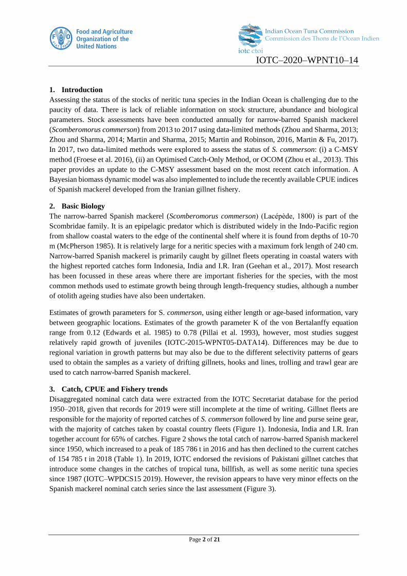
Figure 5 shows the results of the model from the CMSY analysis. Panel A shows the time series of

catches in black and the three-years moving average in blue with indication of highest and lowest catch.

The use of a moving average is to reduce the influence of extreme catches.

Panel B shows the explored r-k values in log space and the r-k pairs found to be compatible with the

catches and the prior information. Panel C shows the most probable r-k pair and its approximate 95%

confidence limits. The probable r values did not span through the full prior range, instead ranging from

0.96–1.48 (mean of 1.19) while probable K values ranged from 389 000 – 801 000 (mean of 558 000).

Given that r and K are confounded, a higher K generally gives a lower r value. CMSY searches for the

most probable r in the upper region of the triangle, which serves to reduce the bias caused by the

triangular shape of the cloud of viable r-k pairs (Ferose et al. 2016).

Panel D shows the estimated biomass trajectory with 95% confidence intervals (Vertical lines indicate

the prior ranges of initial and final biomass). The method is highly robust to the initial level of biomass

assumed (mainly due to the very low catches for the early part of series), while the final depletion range

has a determinative effect on the final stock status. The biomass trajectory closely mirrors the catch

curve with a rapid decline since the late 2000s.

Panel E shows in the corresponding harvest rate from CMSY. Panel F shows the Schaefer equilibrium

curve of catch/MSY relative to B/k. However, we caution that the fishery was unlikely to be in an

equilibrium state in any given year.

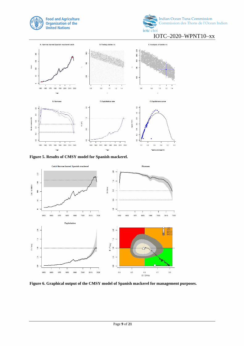
Figure 6 shows the estimated management quantities. The upper left panel shows catches relative to the

estimate of MSY (with indication of 95% confidence limits). The upper right panel shows the total

biomass relative to Bmsy, and the lower left graph shows exploitation rate F relative to Fmsy. The

lower-right panel shows the development of relative stock size (B/Bmsy) over relative exploitation

(F/Fmsy).

The IOTC target and limit reference points for Spanish mackerel have not yet been defined, so the

values applicable for other IOTC species are used. Management quantities (estimated means and 95%

confidence ranges) are provided in Table 3, which shows an average MSY of about 166 000 t. The

KOBE plot indicates that based on the C-MSY model results, Spanish mackerel is currently overfished

(B2018/BMSY=0.96) but is not subject to overfishing (F2018/FMSY = 0.97). The average catch over

the last five years is higher than the estimated MSY. The results are slightly more optimistic than the

last assessment (which suggested the stock was subject to overfishing), as a result of the reduced catches

in the last few years.


of 21

Figure 5. Results of CMSY model for Spanish mackerel.

Figure 6. Graphical output of the CMSY model of Spanish mackerel for management purposes.


of 21

Table 3. Key management quantities from the Catch MSY assessment for Indian Ocean Spanish mackerel. Geometric means (and plausible ranges across all

feasible model runs). n.a. = not available. Previous assessment results are provided for comparison.

Management Quantity 2017 2020

Most recent catch estimate (year) 149 177 t (2015) 154 785 t (2018)

Mean catch – most recent 5 years2 144 724 t (2011 - 2015) 175 891 t (2014 – 2018)

MSY (95% CI) 138 000 (104 000 to 183 000) 166 000 (126 100 – 218 000)

Data period used in assessment 1950 – 2015 1950 – 2018

FMSY (95% CI) 0.60 (0.48 - 0.74) 0.60 (0.48 - 0.74)

BMSY (95% CI) 232 000 (161 000 – 333 000) 277 000 (194 000 – 396 000)

Fcurrent/FMSY (95% CI) 1.19 (0.94 – 2.59) 0.97 (0.78 – 2.14)

Bcurrent /BMSY (95% CI) 0.95 (0.43 – 1.19) 0.96 (0.44 – 1.19)

Bcurrent /B0 (95% CI) 0.47 (0.22 - 0.60) 0.48 (0.22 – 0.60)

2 Data at time of assessment


of 21

5.2. Bayesian Schaefer production model (BSM)

The estimated posterior distributions of r-k for the BSM models 1 – 4 are shown in Figure 7, and the

estimated biomass trend overlaid with CPUE indices (scaled by estimated coachability) for these

models are shown in Figure 8. For Model M3, which made no assumption on the final depletion level,

estimated r-k pairs are located in the tip region of the viable r-k triangle from the CMSY analysis, (

M1

M2

M3

M4

Figure 7–M3). The results are very similar to Model M1, which constrained the final depletion to be in

the medium range of 0.2–0.6 through a penalty function (

M1 M2


of 21

M3

M4

Figure 7–M1). This suggested the medium depletion range appears to be more coherent with the

assumed stock productivity. However, neither model is able to fit the CPUE indices, with the predicted

biomass trend being in opposite direction of the indices (Figure 8 – M1, M3), suggesting the CPUE is

in conflict with model assumptions and/or catch history. For both models, estimated stock status are

very close to be in the centre of the Kobe quadrant (Figure 9 – M1, M3). Both M1 and M3 estimated

F2018 to be 0.99 FMSY; Model M1 estimated B2018 to be 0.97 BMSY and M3 estimated B2018 to be

1.01 BMSY (Table 4). The conclusion of model M1 is similar to the CMSY: the stock is overfished but

is not subject to overfishing.

Additional model configurations were investigated to account for the increasing trend in the CPUE

indices (assuming it is representative of the recent stock trend). Model M2, which assumed a high final

depletion level (0.4 – 0.8) appears to fit the CPUE indices very well (Figure 8 – M2), the model achieved

this by shifting the r-k pairs more towards the higher k and lower r values range (

M1 M2


of 21

M3

M4

Figure 7–M2). Consequently, Model M2 estimated that the stock is in the green KOBE quadrant (Figure

9 – M2), with B2018 estimated to be about 1.29 BMSY and F2018 to be 0.80 FMSY.

Alternatively, Model M4 also fitted the CPUE indices well by assuming a higher process error (twice

the value assumed in other models) (Figure 9 – M4). As such, the model attributed the increase of recent

abundance to other sources of variations of the population which have not been incorporated by the

production function (e.g. recruitment variability, etc.). Model M4 estimated the stock is not overfished

(B2018/BMSY=1.14) but is subject to overfishing (F2018/FMSY=1.02) (Table 4, Figure 8 – M4).


of 21

M1

M2

M3

M4

Figure 7: Results of BDM models 1–4 for Spanish mackerel: posterior estimates of r and K (black dots) and

the 95% CI (the red cross), overlaid with the viable r-k pairs as well as the probable range from the CMSY

analysis (grey dots and the blue cross); right – median and 95% CI of the posterior estimates of biomass,

overlaid with the standardised CPUE indices 2008–2017 with observation errors (red).


of 21

M1

M2

M3

M4

Figure 8: Results of BDM models 1–4 for Spanish mackerel: median and 95% CI of the posterior estimates

of biomass, overlaid with the standardised CPUE indices 2008–2017 with observation errors (red).


of 21

M1

M2

M3

M4

Figure 9: Kobe plots for the BDM models M1 – M4.


of 21


of 21

Table 4: Management quantities from the Bayesian Schaefer production model (BSM) – models 1–4 for Indian Ocean Spanish mackerel, means and 95%

confidence interval.

Management Quantity Model 1 Model 2 Model 3 Model 4

MSY (95% CI) 161 000 t (143 010 – 182 000) 149 000 t (119 010 – 188 000) 156 000 t (130 010 – 186 000) 132 000 t (110 010 – 158 000)

Data period 1950 – 2018 1950 – 2018 1950 – 2018 1950 – 2018

FMSY (95% CI) 0.68 (0.52 – 0.89) 0.38 (0.26 – 0.57) 0.64 (0.45 – 0.90) 0.51 (0.38 – 0.67)

BMSY (95% CI) 238 000 t (197 000– 289 000) 392 000 t (303 000– 508 000) 245 000 t (197 000– 304 000) 262 000 t (209 000– 328 000)

Fcurrent/FMSY (95% CI) 0.99 (0.78 – 1.29) 0.80 (0.66 – 1.11) 0.99 (0.73 – 1.32) 1.02 (0.81 – 1.36)

Bcurrent /BMSY (95% CI) 0.97 (0.75 – 1.23) 1.29 (0.93 – 1.58) 1.01 (0.75 – 1.36) 1.14 (0.86 – 1.44)

Bcurrent /B0 (95% CI) 0.49 (0.37 – 0.62) 0.65 (0.47 – 0.79) 0.50 (0.38 – 0.68) 0.57 (0.43 – 0.72)


of 21

6. Discussion

In this report we have explored two data-limited methods in assessing the status of Indian Ocean

Spanish mackerel: C-MSY and Bayesian Schaefer production model (BSM), both of which are based

on an aggregated biomass dynamic model. The C-MSY requires only the catch series as model input

and uses simulations to locate feasible historical biomass that support the catch history. The BSM has

incorporated time series of relative abundance indices, and estimated model parameters and

management quantities in a Bayesian framework. Estimates from the C-MSY model suggested that

currently the stock of Spanish mackerel in the Indian Ocean is overfished (B2018 < BMSY) but is not

subject to overfishing (F2018 < FMSY). However, it has been demonstrated in many occasions that the

estimates of management quantities of the CMSY analysis are sensitive to assumption of the final stock

depletion.

On the other hand, the BDM model utilised the standardised CPUE indices to provide information on

abundance trend, and as such, the model is less reliant on some of the subjective assumptions. However,

for Spanish mackerel, there appears to be some inconsistency between the CPUE indices, and the catch

history, and productivity assumptions of the species. In order to reconcile the increasing CPUE trend

with the recent high catches, higher levels of stock productivity need to be assumed to allow the stock

to sustain the large catches. Such assumptions tend to lead to more optimistic estimates of current stock

status (e.g. Model M3 estimated the stock to be in green Kobe quadrant when assuming a high final

depletion). Alternatively, the increasing CPUE can be attributed to other (unknow) random variations

in the population (e.g. process error) but there is a risk of overparameterizing the model (such that it

has little predictive power). It remains a question whether the CPUE indices derived from the Iranian

coastal gillnet fleets can index the abundance trend of Spanish Mackerel in the Indian Ocean (the CPUE

has various caveats even as a local index for the Iranian coastal waters, see Fu et al. (2019)).

Nevertheless, the availability of the standardised CPUE as a potential abundance index and its

incorporation in the assessment represents a marked improvement in the development of more robust

methods to assess IOTC neritic tuna species in the context of data deficiency. Future assessments could

consider develop more realistic population models, including age structured models that could utilise

more biological and fishery data beyond simple catch series.


of 21

References

Charnov, E.R., Gislason, H., & Pope, J.P. 2013. Evolutionary assembly rules for fish life histories.

Fish and Fisheries. 14: 213-224.

Carruthers, T.R., Punt, A.E., and Walters, C.J. et al. (2014). Evaluating methods for setting catch

limits in data-limited fisheries. Fisheries Research 153, 48–68.

Froese, R. & Pauly, D., 2015. Fish Base.

Froese, R., Demirel, N., Caro, G., Kleisner, K.M. and Winker, H., 2016. Estimating fisheries

reference points from catch and resilience. Fish and Fisheries, 18 (3). pp. 506-526. DOI

10.1111/faf.12190.

Gislason, H., Daan, N., Rice, J.C. and Pope, J.G. (2010). Size, growth, temperature, and the natural

mortality of marine fish. Fish and Fisheries 11, 149–158.

Ghosh, S., Pillai, N.G.K. & Dhokia, H.K., 2010. Fishery, population characteristics and yield

estimates of coastal tunas at Veraval. Indian Journal of Fisheries, 57(2), pp.7–13.

Hoenig, J.M. 1983. Empirical use of longevity data to estimate mortality rates. Fishery Bulletin 82:

898–903.

IOTC–WPDCS15 2019. Report of the 15th Session of the IOTC Working Party on Data Collection

and Statistics. Karachi, Pakistan, 27-30 November 2019. IOTC–2019–WPDCS15–R[E]: 44

pp.

Jensen, A.L. 1996. Beverton and Holt life history invariants result from optimal tradeoff of

reproduction and survival. Can. J. fish. Aquat. Sci. 53, 820-822.

Kimura, D.K., and Tagart, J.V. 1982. Stock reduction analysis, another solution to the catch

equations. Can. J. Fish. Aquat. Sci. 39: 1467–1472.

Kolody, D., M. Herrera and J. Million. 2011. 1950-2009 Indian Ocean Skipjack Tuna Stock

Assessment (Stock Synthesis). IOTC-2011-WPTT-14(Rev1).

Martell, S. and Froese, R. 2012. A simple method for estimating MSY from catch and resilience. Fish

and Fisheries. 14: 504–514.

Martin, S.M. and Sharma, R., 2015. Assessment of Indian Ocean Spanish mackerel (Scomberomorus

commerson) using data poor catch-based methods. IOTC Secretariat. IOTC-2015-WPNT05-

23.

Martin, S.M. and Robinson, J., 2016. Assessment of Indian Ocean Spanish mackerel (Scomberomorus

commerson) using data poor catch-based methods. IOTC Secretariat. IOTC-2016-WPNT06-18

Rev_1.

Martin, S.M. and Fu, D., 2017. Assessment of Indian Ocean narrow-barred Spanish mackerel

(Scomberomorus commerson) using data-limited methods. IOTC-2017-WPNT07-17.

http://dx.doi.org/10.1111/faf.12190


of 21

Pauly, D. 1980. On the interrelationships between natural mortality, growth parameters, and mean

environmental temperature in 175 fish stocks. J. Cons. Int. Explor. Mer: 175-192.

Geehan, J., Pierre, L., and Fiorellato, F. 2016. Review of the Statistical Data Available for Bycatch

Species. IOTC-2016-WPNT06-07.

Walters, C. Martell, S., and Korman, J. 2006. A stochastic approach to stock reduction analysis. Can.

J. Fish. Aquat. Sci. 63: 212-223.

Schaefer, M.B. 1954. Some aspects of the dynamics of populations important to the management of

commercial marine fisheries. Bulletin, Inter-American Tropical Tuna Commission 1:27-56.

Then, A. Y., Hoenig, J. M., Hall, N. G., and Hewitt, D. A. 2014. Evaluating the predictive performance

of empirical estimators of natural mortality rate using information on over 200 fish species. –

ICES Journal of Marine Science, doi: 10.1093/icesjms/fsu136.

Zhou S.J., Yin S.W., James T.T., Anthony D.M.S., and Michael F. (2012) Linking fishing mortality

reference points to life history traits: an empirical study. Canadian Journal of Fisheries and

Aquatic Science 69, 1292-1301. doi:10.1139/F2012-060.

Zhou, S., Pascoe, S., Dowling, N., Haddon, M., Klaer, N., Larcombe, J., Smith, A.D.M., Thebaud, O.,

and Vieira, S. 2013. Quantitatively defining biological and economic reference points in data

poor and data limited fisheries. Final Report on FRDC Project 2010/044. Canberra, Australia.

Zhou, S., Chen, Z., Dichmont, C.M., Ellis, A.N., Haddon, M., Punt, A.E., Smith, A.D.M., Smith, D.C.,

and Ye, Y. 2016. Catch-based methods for data-poor fisheries. Report to FAO. CSIRO,

Brisbane, Australia.

Zhou, S. and Sharma, R. 2013. Stock assessment of two neritic tuna species in Indian Ocean: kawakawa

and longtail tuna using catch based stock reduction methods. IOTC Working Party Paper.

IOTC–2013–WPNT03–25.

Zhou, S. and Sharma, R. 2014. Stock assessment of neritic tuna species in Indian Ocean: kawakawa,

longtail and narrow-barred Spanish mackerel using catch based stock reduction methods. IOTC

Working Party Paper. IOTC–2014–WPNT04–25.

assessment of indian ocean narrow-barred spanish mackerel

Documents