assessment of hydro-morphological response of …
TRANSCRIPT

i
ASSESSMENT OF HYDRO-MORPHOLOGICAL RESPONSE OF SELECTED
REACH OF THE JAMUNA RIVER DUE TO STRUCTURAL INTERVENTION
USING DELFT3D MODEL
MD. ZAKIR HASAN
Student No.: 0412162004P
DEPARTMENT OF WATER RESOURCES ENGINEERING
BANGLADESH UNIVERSITY OF ENGINEERING AND TECHNOLOGY
(BUET)
Dhaka, Bangladesh
September, 2018

ii
ASSESSMENT OF HYDRO-MORPHOLOGICAL RESPONSE OF SELECTED
REACH OF THE JAMUNA RIVER DUE TO STRUCTURAL INTERVENTION
USING DELFT3D MODEL
A THESIS SUBMITTED TO THE DEPARTMENT OF WATER RESOURCES
ENGINEERING IN PARTIAL FULFILLMENT OF THE REQUIREMENTS FOR THE
DEGREE OF MASTER OF SCIENCE IN WATER RESOURCES ENGINEERING
SUBMITTED BY
MD. ZAKIR HASAN
DEPARTMENT OF WATER RESOURCES ENGINEERING
BANGLADESH UNIVERSITY OF ENGINEERING AND TECHNOLOGY
(BUET)
Dhaka, Bangladesh
September, 2018

i

ii

iii
TABLE OF CONTENTS
Page No.
Certification of Approval i
Declaration ii
Table of Contents iii
List of Figures vii
List of Tables x
List of Symbols xi
List of Abbreviation xii
Acknowledgement xiii
Abstract xiv
CHAPTER 1: INTRODUCTION 1
1.1 General 1
1.2 Background of the Study 1
1.3 Objectives of the Study 3
1.4 Structure of the Thesis 3
CHAPTER 2: LITERATURE REVIEW 4
2.1 General 4
2.2 River Bank Erosion 4
2.3 Sediment Transport 5
2.4 Previous Studies on Hydro-Morphology of the Jamuna River 5
2.5 Previous Studies on Structural Intervention in a River 10
2.6 Previous Studies on Mathematical Modelling 11
2.7 Previous Studies on Delft3D Model 13
2.8 Study Area 15
2.8.1 The Jamuna River System 17
2.8.2 Source and Course of the River 17
2.8.3 Catchment Characteristics 18
2.8.4 Topography of the Catchment Area 19
2.8.5 Sediment Characteristics 20
2.8.6 Hydraulic Characteristics of the Jamuna 20

iv
CHAPTER 3: THEORETICAL BACKGROUND 22
3.1 General 22
3.2 Hydrodynamics of a River 22
3.3 Morphology of a River 23
3.4 Structural Intervention in a River 24
3.4.1 Marginal Embankments/Levees 24
3.4.2 Guide Bank 25
3.4.3 Revetments 25
3.4.4 Groynes/Spurs 26
3.4.4.1 Length of Groynes/Spurs (Lg) 27
3.4.4.2 Spacing between Groynes/Spurs (Sg) 27
3.5 Structural Intervention in the Jamuna River 28
3.5.1 Groynes/Spurs 28
3.5.2 Revetments and Hard points 29
3.6 River Response 32
3.6.1 River Responses Type 32
3.6.2 Qualitative Response 33
3.7 Mathematical Modeling 34
3.8 Delft3D Model 35
3.8.1 Numerical Aspects of Delft3D-FLOW 35
3.8.1.1 Staggered grid 36
3.8.1.2 Definition of model boundaries 37
3.8.2 Hydrodynamic equations 38
3.8.2.1 The σ co-ordinate system 39
3.8.2.2 Cartesian co-ordinate system in the vertical (Z-model) 40
3.8.2.3 Continuity equation 41
3.8.2.4 Momentum equations in horizontal direction 42
3.8.2.5 Vertical velocities 43
3.8.3 Transport equations 43
CHAPTER 4: DATA COLLECTION AND METHODOLOGY 46
4.1 General 46
4.2 Work Analysis and Preparing Work Plan 46
4.3 Data Collection 48
v
4.3.1 Hydrometric Data 48
4.3.2 Bathymetric Data 50
4.3.3 Satellite Image 51
4.3.4 Sediment Data 51
4.3.5 Field Visit and Bed Sample Collection 52
4.4 Methodology 54
4.5 Model Setup 54
4.5.1 RGFGRID 56
4.5.2 QUICKIN 56
4.5.3 QUICKPLOT 57
4.5.4 Dry Points 58
4.5.5 Thin Dams 58
4.5.6 Modeling Framework 59
4.5.7 Space and Time Variation 60
4.5.8 Model Stability Check, Calibration and Validation 60
4.5.9 Different Option Simulation 61
4.5.10 Data Extraction 62
CHAPTER 5: MODEL SET UP FOR SELECTED REACH OF THE JAMUNA RIVER 63
5.1 General 63
5.2 Model Setup for Selected Reach of the Jamuna River 63
5.2.1 Grid Generation 64
5.2.2 Bathymetry 64
5.2.3 Boundary Conditions 65
5.2.4 Additional Parameters 68
5.2.5 Model Calibration 68
5.2.6 Model Validation 70
5.2.7 Morphological Calibration of the Model 71
5.2.8 Comparison of Simulated Water Level between MIKE21C and Delft3D 74
5.2.9 Model Stability Analysis 75
5.3 Model Simulation with Different Options 75
CHAPTER 6: RESULTS AND DISCUSSIONS 86
6.1 General 86
6.2 Observation of Hydrodynamic Parameters 86

vi
6.2.1 Velocity Vectors 88
6.2.2 Depth Averaged Velocity 93
6.2.2.1 Bank Line Velocity 98
6.2.3 Bed Shear Stress 99
6.2.3.1 Bank Line Bed Shear Stress 101
6.3 Observation of Morphologic parameters 102
6.3.1 Cumulative Erosion/Deposition Curves 103
6.3.2 Bed Level Variation at Different Locations 106
6.3.2.1 Bed Level Variation across the River for Option 2 108
6.3.2.2 Bed Level Variation along the River for Option 2 110
6.3.2.3 Bed Level Variation across the River for Option 4 and Option 6 112
6.3.2.4 Bed Level Variation along the River for Option 4 and Option 6 113
6.4 Summary of the Results 115
CHAPTER 7: CONCLUSIONS AND RECOMMENDATIONS 119
7.1 General 119
7.2 Conclusions 119
7.3 Recommendations for Further Study 120
REFERENCES 121
APPENDIX-A: Model output for different parameters
APPENDIX-B: Model simulated cross-sections at different locations
APPENDIX-C: Model output in tabular forms for various option simulations

vii
LIST OF FIGURES Figure 2.1: Study area along the Jamuna River (Source: CEGIS, 2012) 16 Figure 2.2: Brahmaputra-Jamuna River System within Bangladesh Territory 19 Figure 3.1: River Classification by Brice 24 Figure 3.2: Typical cross-sections of levees for different heights 25 Figure 3.3: Components of a revetment on riverbank 26 Figure 3.4: Types of groynes based on alignment 27 Figure 3.5: Permeable groune for Jamuna Bank protection At Kamarjani (FAP21/22) 29 Figure 3.6: Permeable groune for Jamuna Bank protection At Kamarjani 30 Figure 3.7: Lane‟s balance (Source: Sarker, 2008) 34 Figure 3.8: Example of a grid in Delft3D-FLOW 36 Figure 3.9: Mapping of physical space to computational space 36 Figure 3.10: Grid staggering, 3D view (left) and top view (right) 37 Figure 3.11: Example of Delft3D model area 38 Figure 3.12: Definition of water level (ζ), depth (h) and total depth (H) 40 Figure 3.13: Example of σ- and Z-grid 41 Figure 4.1: Flow chart showing the entire methodology 47 Figure 4.2: Historical water level data at Sirajganj hard point 49 Figure 4.3: Historical discharge hydrographs at Bahadurabad station 50 Figure 4.4: Bathymetric data of 50 km reach of the Jamuna River 51 Figure 4.5: Grain size distribution of sample 1 52 Figure 4.6: Grain size distribution of sample 2 52 Figure 4.7: Hjulstrӧms diagram (Hjulstrӧm, 1935) 53 Figure 4.8: Title window of Delft3D 55 Figure 4.9: Graphic User Interface (GUI) of Delft3D 55 Figure 4.10: RGFGRID and QUICKIN window 57 Figure 4.11: Structure of Delft3D 57 Figure 4.12: Sub-data group Dry points 58 Figure 4.13: Equivalence of v-type thin dams (left) and u-type thin dams (right) with the same grid indices, (M 1 to M+1, N) 59 Figure 5.1: Computational Grid cell of Jamuna River in the study area 64 Figure 5.2: Model bathymetry of Jamuna River in the study area 65 Figure 5.3: Upstream and downstream boundaries of the model 66 Figure 5.4: Flow conditions applied at upstream boundary of the model 67 Figure 5.5: Downstream water level boundary for the model 67 Figure 5.6: Comparison of model simulated and observed water levels of Jamuna River at Sirajganj for different ‘n’. 69 Figure 5.7: Comparison of model simulated and observed water levels of Jamuna River at Sirajganj for the monsoon of 2012 69 Figure 5.8: Calibration of the model at Bangabandhu Bridge site for water level 70 Figure 5.9: Validation of the model simulated and observed water level data at Sirajganj for the year 2013 71 Figure 5.10: Flow discharge vs. observed sediment discharge graph at Bahadurabad 72 Figure 5.11: Flow discharge vs. simulated sediment discharge graph at Sirajganj 72 Figure 5.12: Comparison of cross-sections at SHP for pre-monsoon 2011 with diffusivity 1 73 Figure 5.13: Comparison of cross-sections at SHP for pre-monsoon 2011 with diffusivity 5 73 Figure 5.14: Comparison of cross-sections at SHP for pre-monsoon 2011 with diffusivity 10 73

viii
Figure 5.15: Comparison of simulated WL data between MIKE21C and Delft3D in 2012 at Sirajganj 74 Figure 5.16: Erosion prone areas at the right bank of the Jamuna River 76 Figure 5.17: Base (without any structure) 78 Figure 5.18: Option 1 (Single groyne) 79 Figure 5.19: Option 2 (2 groynes with S/L ratio 1.0) 80 Figure 5.20: Option 3 (2 groynes with S/L ratio 1.5) 81 Figure 5.21: Option 4 (2 groyne with S/L ratio 2.0) 82 Figure 5.22: Option 5 (3 groyne with S/L ratio 1.0) 83 Figure 5.23: Option 6 (3 groyne with S/L ratio 1.5) 84 Figure 5.24: Option 7 (3 groyne with S/L ratio 2.0) 85 Figure 6.1: Water level at different dates for 2 groynes with S/L = 1.5 86 Figure 6.2: Depth averaged velocities at different dates for 2 groynes with S/L = 1.5 87 Figure 6.3: Bed shear stress at different dates for 2 groynes with S/L = 1.5 87 Figure 6.4: Velocity vectors from model output for (a) Base, (b) Option 1, (c) Option 2, (d) Option 3, (e) option 4, (f) Option 5, (g) Option 6 and (h) Option 7 92 Figure 6.5: Relative comparison of velocity variation at groyne u/s for different options 94 Figure 6.6: Relative comparison of velocity variation at groyne d/s for different options 94 Figure 6.7: Relative comparison of velocity variation at groyne SHP for different options 95 Figure 6.8: Relative comparison of velocity variation at groyne BBS for different options 95 Figure 6.9: Comparison of velocity with base at the u/s of 1st groyne for option 2 96 Figure 6.10: Comparison of velocity with base at the d/s of 1st groyne for option 2 96 Figure 6.11: Comparison of velocity with base at the u/s of 2nd groyne for option 2 97 Figure 6.12: Comparison of velocity with base at the d/s of 2nd groyne for option 2 97 Figure 6.13: Comparison of bank line velocities for different spacing of groynes 98 Figure 6.14: Relative comparison of bed shear stress at groyne u/s for different options 99 Figure 6.15: Relative comparison of bed shear stress at groyne d/s for different options 99 Figure 6.16: Relative comparison of bed shear stress at groyne SHP for different options 100 Figure 6.17: Relative comparison of bed shear stress at groyne BBS for different options 100 Figure 6.18: Comparison of bed shear stress along the bank line for different spacing of groynes 101 Figure 6.19: Cum. erosion/sedimentation at different dates for 2 groynes with S/L = 1.5 102 Figure 6.20: Total transport at different dates for 2 groynes with S/L = 1.5 102 Figure 6.21: Relative comparison of cum. erosion/deposition at groyne u/s for different options 104 Figure 6.22: Relative comparison of cum. erosion/deposition at groyne d/s for different options 104 Figure 6.23: Relative comparison of cum. erosion/deposition at groyne SHP for different options 105 Figure 6.24: Relative comparison of cum. erosion/deposition at groyne BBS for different options 105 Figure 6.25: Cross-section locations to observe bed level variation across and along the river for option 2 106 Figure 6.26: Cross-section locations to observe bed level variation across and along the river for option 4 and 6 107 Figure 6.27: Bed level variation along the 1st groyne with respect to base for option 2 (Section a-a) 108 Figure 6.28: Bed level variation along the 2nd groyne with respect to base for option 2 (Section c-c) 109 Figure 6.29: Bed level variation between the 1st and 2nd groyne with respect to base for option 2, option 3 and option 4 (Section b-b) 109 Figure 6.30: Bed level variation along the river in front of the nose of the groynes with respect to base for Option 2 (S/L = 1.0) (Section 1-1) 110 Figure 6.31: Bed level variation along the river in front of the nose of the groynes with respect to base for Option 4 (S/L=2.0) (Section 1-1) 111
ix
Figure 6.32: Bed level variation between the 1st and 2nd groyne with respect to base for option 4 (Section a-a) 112 Figure 6.33: Bed level variation between the 2nd and 3rd groyne with respect to base for option 6 (Section a-a) 112 Figure 6.34: Bed level variation along the river in front of the nose of the groynes with respect to base for Option 4 (2 groynes with S/L = 2.0) (Section 1-1) 113 Figure 6.35: Bed level variation along the river along the nose of the groynes with respect to base for Option 6 (3 groynes with S/L = 1.5) (Section 1-1) 113 Figure 6.36: Bed level variation along the river in front of the nose of the groynes with respect to base for Option 6 (3 groynes with S/L = 1.5) (Section 1-1) 114

x
LIST OF TABLES
Table 2.1: Summary of hydraulic characteristics of the Jamuna River 21 Table 3.1: List of various structural intervention in Brahmaputra/Jumna and the present status 31 Table 4.1: Available Water Level & Discharge Data 48 Table 4.2: Status of collected sediment data of the Jamuna River 51 Table 4.3: Simulation of the model with different options 61 Table 5.1: Summary of the parameters used for the model of Jamuna River 68 Table 5.2: Stability analysis results of the model 75 Table 5.3: Description of the simulation options 77 Table 6.1: Change of parameters with respect to base condition at u/s for various options (July) 116 Table 6.2: Change of parameters with respect to base condition at d/s for various options (July) 116 Table 6.3: Change of parameters with respect to base condition at SHP for various options (July) 117 Table 6.4: Change of parameters with respect to base condition at BBS for various options (July) 117 Table 6.5: Monthly variation of cum. erosion/deposition at different locations for all the options 118

xi
LIST OF SYMBOLS
d50 Size of bed material load
Fx Horizontal stress
Fy Vertical stress
g Acceleration due to gravity
H Water level
HFL High flood level
h Water depth
i Channel slope
L Length of groyne
n Manning’s roughness coefficient
Px Horizontal pressure
Py Vertical pressure
Q Discharge
Qs Sediment discharge
S Spacing of groynes
SHW Shallow water
U Horizontal component of velocity
V Vertical component of velocity
x, y Cartesian coordinate system
z Bed level
ρ Density of water
𝑣𝑣 Eddy viscosity

xii
LIST OF ABBREVIATIONS
ADCP Acoustic Doppler Current Profiler
BBS Bangabandhu Bridge Site
BIWTA Bangladesh Inland Water transport Authority
BWDB Bangladesh Water Development Board
CEGIS Center for Environment and Geographic Information Services
Delft 3D Three-dimensional model developed by Delft hydraulics
DHI Danish Hydraulic Institute
D/S Downstream
FAP Flood Action Plan
GBM Ganges Brahmaputra Meghna
GUI Graphic User Interface
HEC-RAS Hydraulic Engineering Center- River Analysis System
IWM Institute of Water Modelling
MIKE 21C Two-dimensional One Layer Curvilinear Model Develop by MIKE ABBOTT
PWD Public Works Department
SHP Sirajganj Hard Point
U/S Upstream
WARPO Water Resources Planning Organization

xiii
ACKNOWLEDGEMENT
All praises are due to the Almighty Allah who has provided me with the opportunity to complete this research. The author acknowledges his deepest gratitude to his supervisor Dr. Md. Abdul Matin, Professor, Department of Water Resources Engineering, BUET for providing me such an interesting idea for the thesis work and encouraging working with it. His cordial supervision, valuable suggestion and unfailing eagerness made the study to a successful work.
The author is also grateful to Dr. Mostofa Ali, Professor & Head, Department of Water Resources Engineering, BUET, Dr. A.T.M Hasan Zobeyer, Associate Professor, Department of Water Resources Engineering, BUET and Dr. Faruq Ahmed Mohiuddin, Senior Water Resources Specialist, IWM, who were the members of the board of examiners. Their valuable comments on this thesis are duly acknowledged. The author would like to thank his family members for their encouragement and inspiration. The author is grateful for their guidance and blessings. Without their help and support and sacrifice the author wouldn’t have finished his M.Sc. Engg. The author is very much thankful to Mr. Tanvir Ahmed, M.Sc. student, IHE, Netherlands for his help and support to do this work. The author is pleased to Md. Musfequzzaman, Associate Specialist, IWM and Shampa, PhD student, Kyoto University, Japan for their inspiration and support. The author is indebted to Institute of Water Modelling (IWM), Center for Environmental and Geographic Information Services (CEGIS) and officials of Bangladesh Water Development Board (BWDB) Sirajganj, for providing necessary information and data to carry out this research work. Md. Zakir Hasan September 2018

xiv
ABSTRACT
In this study, an attempt has been made to analyze the hydro-morphological responses
of the Jamuna River due to structural intervention in a selected reach by preparing a
morphological model. The study reach covers from 30 km upstream of Bangabandhu
Bridge (BB) to 20 km downstream of this bridge. A two-dimensional mathematical
model has been developed using Delft3D and studied various options with structural
intervention of groyne(s) along a selected reach in the right bank of the Jamuna River
at the upstream of Sirajganj Hard Point (SHP). The model has been calibrated and
validated against the data for the year 2012 and 2013 respectively. Then simulations
have been done with seven different options consist of groynes with various number
and spacing. The length of the groynes have been selected as about one-fourth of the
channel width. The spacing and length ratio (S/L) of the groynes have been set as 1.0,
1.5 and 2.0 respectively for the option simulations. In order to quantify the response of
the river hydrodynamics and morphology for various options at different locations,
model results for the month of July have been assessed. All the model output have been
presented and discussed. For the purpose of discussion and interpretation of model
output, four points as the upstream of the structure (u/s), downstream of the structure
(d/s), Sirajganj Hard Point (SHP) and Bangabandhu Bridge Site (BBS) have been taken
into consideration. Model results show that at the upstream of the selected intervention,
water level increases about 10.84% and for the downstream is 6.72%. This rise of water
level may be for the afflux effect due to the structural intervention(s). The velocity and
bed shear stress show decreasing tendency around the structures which indicates the
attainment of siltation zone. The effects are considerable at the upstream and
downstream of the groyne(s) and for the other two points (e.g. Sirajganj Hard Point
and Bangabandhu Bridge Site) the effect is very little due to the long distance. From
the velocity vectors and bank line velocities as well as bed shear stress, it can be
decided that for this specific reach of the river, the maximum allowable spacing
between the groynes is 2.0 times of its length. Otherwise the bank will be in vulnerable
condition due to erosion. The bed level variation surrounding the groynes is
considerable. The effect of groyne extends up to 1 km inside the river and 2 km laterally

xv
from either nose of the groyne. The maximum erosion is -5.25 m and deposition is
+3.70 m along the length of the groyne. In case of lateral section (along the river) the
values are -6.0 m and +4.0 m respectively.
For the structures, the near bank velocity and bed shear stress become very small with
the increasing number of intervention. Thus it can be said that to prevent the bank
erosion, this types of structures with increasing numbers and different spacing provides
satisfactory results. Overall, the model results show that it has the capacity to assess
the hydro-morphological river responses for various options particularly at the vicinity
of the interventions.

1
CHAPTER 1
INTRODUCTION
1.1 General
Structural intervention in a river is a major part of river training and bank protection. Being
one of the most vital rivers in Bangladesh, the Jamuna experiences severe bed and bank
erosion every year. Sometimes, steps are taken to prevent such type of troubles but in many
cases the projects fail for the unpredictable behavior of the Jamuna River. To adress the
problems two-dimensional hydrodynamic and morphological model is being used as a
functional tool now a days. Delft3D is such type of modeling software to analyze river
responses at different conditions. In this study, analysis of the selected erosion prone reach of
the Jamuna River has been done with structural intervention like groynes and compare the
results with the free flow condition. Thus relationship among different hydrodynamic and
morphological parameters have been established for different conditions that might help the
planners, engineers and implementing authorities in future to work on the Jamuna River.
1.2 Background of the Study
The Jamuna River in Bangladesh is one of the world’s largest and most geomorphologically
active braided alluvial rivers (Mosselman, 2006). The length of the Jamuna is about 2900 km
originated from the Himalayas and has a drainage area of 573,500 km2. The length of the river
is almost 240 km inside of Bangladesh. The overall width of the River varies spatially and
temporally, from 6 to 14 km. There exits different types of channel within the overall width
of the river (Rahman, Mahmud and Uddin, 2012). Movement of bars and branches
(Schuurman, Kleinhans and Middelkoop, 2016), river bank erosion, bank lines shifting in
the scale of several hundred meters to a few kilometers in a year is common in the river
(Ahmed and Hasan, 2011). Main channels in this river shift from one side to another thus
experience bed level changes over the period. The bed level changes over a year can be several
meters locally. On the other hand, main stream flows along the river bank in many locations
that generates excess near bank velocity, which causes seasonal bank erosion for particular
locations (Musfequzzaman, 2012). Bank erosion in the Jamuna River is one of the major
problems in Bangladesh. Thousands of people become homeless every year and they lose their

2
homestead and croplands. Mosques, schools, hospitals and other infrastructures are damaged
due to erosion into the mighty Jamuna River (Urmilaz, 2012). The west bank of the Jamuna
River commonly known as Brahmaputra Right Embankment (BRE) is most vulnerable to this
kind of problem. Moreover, Bangabandhu multipurpose bridge, the most vital bridge in
Bangladesh is situated in the Jamuna River. In addition, Sirajganj district town with some
industrial area is situated beside the Jamuna River. So the vulnerability of the bank of the
Jamuna River is a major concern in the country as it is related to different social and economic
activities of great worth. That’s why training of the Jamuna River always gets priority to the
implementing authority like Bangladesh Water Development Board (BWDB), Bangladesh
Inland Water Transport Authority (BIWTA) to protect the river banks and river bed also. Many
river training structures like gabions, submerged vanes, hard points and groynes have been
used to protect the river banks especially at river bends (FAP21/22, 2001; Abbas, B. G.,
Mojtaba, 2009). Different pre and post studies and analyses have been done to sustain the right
bank of the Jamuna. Various types of physical and mathematical model studies have been
being done in relation to academic and professional purposes.
In the recent years, mathematical models have been increasingly used including
hydrodynamics, sediment transport and morphological processes in different types of rivers
(Dargahi, 2004; Nicholas, 2013; Yang, Lin and Zhou, 2015) since the physical model study is
expensive and time consuming also. Several researches like assessment of river
hydrodynamics and morphology (Urmilaz, 2012; Roy, 2015), impact of river dredging
(Musfequzzaman, 2012; Alam and Matin, 2013) have been done using the modeling tool.
However, study on river analysis with structural intervention using model is limited.
In this study, assessment has been done for change in the hydrometric parameters as well as
morphologic scenarios for the selected reach of the Jamuna River due to transverse structures
(groynes/cross bars) using a two-dimensional hydrodynamic model. Single and series of
transverse structures have been placed in the erosion prone areas at different spacing along the
right bank of the Jamuna River and model has been simulated using Delft3D model to observe
the impact at bed and bank of the river as well as the adjacent Sirajganj town.

3
1.3 Objectives of the Study
The objectives of the study are as follows:
i. To set up a two-dimensional hydrodynamic model with Delft3D for 50 km reach of
the Jamuna River
ii. To assess the hydrodynamic response of the river for different inflow conditions for
structural interventions (groynes/cross bars) in right bank of the river
iii. To analyze the response of river bed under study due to structural intervention
(groynes/cross bars)
1.4 Structure of the Thesis
The thesis has been organized under seven chapters. Chapter 1 describes the background and
objectives of the study. Chapter 2 describes different definition of relevant topics, literatures,
previous studies related to this study. Chapter 3 describes theoretical background of tools used
in this thesis work. Chapter 4 describes the data collection and its processing followed by data
analysis and also methodology of the thesis. Chapter 5 illustrates the model set up for the study
area. Chapter 6 presents the results of the study from different points of view and few
discussions of these results are also discussed. Chapter 7 states the concluding points and
recommendations for further study.

4
CHAPTER 2
LITERATURE REVIEW
2.1 General
Bangladesh is dominated by three great rivers – the Brahmaputra-Jamuna, the Ganges and the
Meghna – that combine to feed sediment into one of the World’s largest deltas in the Bay of
Bengal (Best et al., 2007).The Brahmaputra, one of the largest braided rivers in the world,
originates from the Himalayas and enters Bangladesh at Kurigram as Jamuna. Though the
history of the Jamuna is not more than 250 years, it shows severe changes in its course due to
natural and anthropogenic influences (Urmilaz, 2012). Due to the unpredictability, training of
this river for mankind is so tough. That’s why, a lot of studies and researches have been done
related to the Jamuna River for different purposes. The summaries of different works and
studies relevant to this study as well as some related terminologies has been discussed in the
following articles.
2.2 River Bank Erosion
Riverbank erosion is an endemic and recurrent natural hazard. When rivers enter the mature
stage they become sluggish and meander or braid. These oscillations cause massive riverbank
erosion. The intensity of bank erosion varies widely from river to river as it depends on such
characteristics as bank material, water level variations, nearbank flow velocities, planform of
the river and the supply of water, sediment into the river and so on. For example, loosely
packed, recently deposited bank materials, consisting of silt and fine sand, are highly
susceptible to erosion. Rapid recession of floods accelerates the rates of bank erosion in such
materials. Rivers belong to dynamic systems as they are continuously changing their way.
Erosion and accretion is a natural process for any river. Though, sometimes erosion exceeds
accretion and cause havoc in lives and livelihoods, mostly the poor society become the
worst casualty. Riverbank erosion occurs both naturally and through human interference. The
natural riverbank erosion process can produce favorable outcomes such as the formation
of productive floodplains and alluvial terraces. Even stable rivers may have some amount
of erosion. However, unstable rivers and the erosion that take place beyond normal range on

5
either bank is a serious concern. Environmental refugees are one of the most burning issues
at this time all over the world (Hoque Mollah and Ferdaush, 2015).
2.3 Sediment Transport
Sediment transport is the movement of solid particles, typically due to a combination of the
gravity force acting on the sediment, and/or the movement of the fluid in which the
sediment is entrained. An understanding of sediment transport is typically used in natural
systems, where the particles are clastic rocks (sand, gravel, boulders, etc.), mud, or clay.The
fluid is air, water, or ice; and the force of gravity acts to move the particles due to the sloping
surface on which they are resting. Sediment transport due to fluid motion occurs in rivers,
the oceans, lakes, seas, and other water bodies, due to currents and tides; in glaciers as they
flow, and on terrestrial surfaces under the influence of wind (Urmilaz, 2012). The ability of
the channel to entrain and transport sediment depends on the balance between gravitational
forces acting to settle particles on the bed and drag forces that act to either suspend them in
the flow or shove them along downstream.
The dynamic problems of liquid-solid interaction are greatly influenced by the sediment
properties. The description of the latter, however, is exceedingly complex and one is forced to
make many simplifying assumptions. The first of which is the subdivision into cohesive and
non-cohesive sediments. In cohesive sediments the resistance to erosion depends on the
strength of the cohesive bond between the particles which may far outweigh the influence of
the physical characteristics of individual particles. The problem of erosion resistance of
cohesive soils is a very complex one and at present our understanding of the physics of it is
very incomplete. The non-cohesive soils generally consist of larger discrete particles than
cohesive soils and the movement of these particles depends on the physical properties of the
individual particles, such as size, shape and density (Hassanzadeh, 2012).
2.4 Previous Studies on Hydro-Morphology of the Jamuna River
(Uddin and Rahman, 2012) Investigated the flow processes into the scour hole near a bank
protection work. A revetment-like structure (hard point) was selected in the Jamuna River for
that study. Acoustic Doppler Current Profiler (ADCP) was used to measure the hydraulic data
into the scour hole. The measured hydraulic data was analyzed and represented by velocity
vectors.
6
(Best et al., 2003) worked with the three-dimensional subsurface alluvial architecture of a
large (approximately 3 km long, 1 km wide, 12 m high), mid-channel sand braid bar in the
Jamuna River, Bangladesh. Evolution of the bar and its depositional characteristics were
assessed from a unique combination of ground-penetrating radar surveys, vibracoring, and
trenching that were allied to a series of bathymetric surveys taken during growth of the bar
over a 29-month period. The methodology permitted identification of the formative processes
of different packages of braid-bar sedimentation and provided a facies model for deposition
within the entire bar. Finally the authors suggested a scale invariance in several aspects of
mid-channel bar sedimentation in sand-bed rivers and proposes a model of braid-bar
sedimentation that may be applied widely within studies of braided alluvial architecture.
(Musfequzzaman, 2012) investigated the river responses due to dredging on a selected reach
of the Jamuna River by preparing a morphological model of this river. The study reaches was
from 30 km upstream of Bangabandhu Bridge to 20 km downstream of this bridge. At first
the two idealized test channels i.e. straight and meandering channels were modeled and
the results were explored for better understanding the theoretical response of river due
to dredging. The both idealized test channels were 15 km long and 1 km wide. The
conveyance areas of these channels were kept similar to the channel in front of Sirajganj
Hard Point. To setup these morphological models, MIKE21C, an advanced two-
dimensional mathematical modelling software developed by DHI, was applied and numbers
of simulations were conducted for different dredging conditions to fulfill the study
objectives. From analyses, the author found in idealized test channels that with the
increasing of dredging depth as well as with the dredging width, dimensionless velocity
increases along the dredged channel and decreases along the bank. Similar incidences were
observed also in Jamuna model that along the dredged channel the dimensionless velocity
increases with the increase of relative dredging depth. It was also observed comparing
the model results with Shield diagram that the bed materials along bank remain at the
boundary of erosive and non-erosive zone during average velocity of Jamuna. With
higher dredging depth condition, the velocity along bank decreases in such an amount
so that it becomes lower than the critical velocity and the bank becomes non erosive zone.
In Jamuna River, bed scour near Sirajganj Hardpoint decreases maximum 33.4% for 7 m of
dredging depth and average rate of decreasing of bed scour is 5.5 % per meter of
dredging depth. However, if dredging executed near Sirajganj Hardpoint, the channel became
wider as the dredging depth increases. Finally, it was found that the bank erosion decreases

7
with the increasing of dredging depth. In some point the bank erosion decreases about 50m
due to dredging.
(Urmilaz, 2012) Simulated the sediment transport rate at the river Jamuna and variation of bed
level along the river using a two dimensional morphological model. Non-cohesive sediment
transport module of Delft 3D Flow was used for the simulation. The upstream boundary of
the model was taken at 30 km upstream of Bangabandhu Bridge and downstream boundary
was taken at 20 km downstream of Bangabandhu Bridge. Simulation period was taken
from April 2010 to December 2012. Simulation was carried out for hydrodynamic calibration
and for sediment transport rates. The cross-sections were taken at the locations that are
vulnerable, such as Subaghacha, Sirajganj, Jamuna Bridge and also in the upstream near
Kazipur and downstream near Chauhali etc. In the Morphology tab, the morphological scale
factor was set to 8.25 which extend the 121 days hydrodynamics to about 1000 days of
morphological change. Calibration and validation were carried out against field observations
(water level) of 2010 and 2011 respectively. Comparisons between simulated and observed
water level were taken at the Sirajganj station. The results showed satisfactory agreement
with observed values. For hydrodynamic and morphological computation, a time series
discharge data was used at the upstream boundary and water level data as downstream
boundary. Observed and simulated bed level elevation of 2010 was compared and the
comparison showed a very good agreement. After calibration of the model, the net
amount of erosion and deposition along the river reach was computed. Finally, cross-sectional
variation of bottom level during the monsoon seasons from 2010 to 2012 was observed.
Results revealed that erosion takes place in the channel bed and the deposition mainly takes
place to the adjacent char areas and increased its width and area. It was also evident
that the channel has been shifted westwards of the reach due to shifting of the bank line of the
river. Many tributary and distributaries were appeared due to progressive erosion. In
Sirajganj, the sediment transport capacity seemed to be the highest due to higher
velocity of flow. The zones of higher velocity has higher sediment transport capacities
therefore occurs more erosion.
(Ahmed and Hasan, 2011) observed the flow pattern around the Sirajganj Hard point
setting up a 2D hydrodynamic model of 50 km river reach of the Jamuna (30 km upstream
and 20 km downstream of Jamuna Bridge). The model was expanded to determine the
scenario of inundation depth, inundation area and velocity of flood flow also. Satellite
image analysis was also performed to determine plan form and bank line shifting of

8
the river. There was a continuous shifting of bank line and the formation of embayment at
the upstream of the hard point. The flow attacked the hard point at an oblique direction.
Bed shear stress at the front of falling apron was found much higher than the critical
bed shear stress. Again the flow was slightly converged along the hard point. So scour hole
were formed in front of the falling apron. Though it did not exceed the design scour
depth, some flow slides occurred during the fast scouring process due to excessive
mica content which has low relative density. The apron material could not get sufficient
time for its settlement on the quickly developed scour hole resulting in the failure of the hard
point. The main cause of flood around Sirajganj town was the formation of breaches in
Brahmaputra Right Embankment (BRE). As the topography of Sirajganj town is lower than
the peak flood level of the Jamuna, failure of BRE caused flooding in Sirajganj town
and the area around it and damaged to lives and properties. In 2007 flood events, The
average inundation depth was 0.6-1.0 m. Maximum inundation depth in few areas of town
was around 2.0 m. average velocity of flood water in town area was 0.3-0.4 m/s.
(Ali, 2004) Conducted a morphological analysis of the Jamuna River using finite element
method. RMA2, a hydrodynamic model and SED2D, a sediment transport model, were used
to simulate the morphology of the Jamuna. Models had been applied using SMS (Surface-
water Modeling System) environment, which gave the pre and post-processing options for
input and output data. The finite element mesh was developed using LANDSAT image of the
17th November 2000. Initial bed elevations for the nodes of the mesh had been composed from
the scattered survey data of April 2001 by BIWTA. Once the mesh and bathymetry had been
obtained, the models were ready thereby to incorporate boundary conditions, initial conditions
and material properties. The hydrodynamic model developed in the study was satisfactorily
calibrated and validated against the observed water surface elevations at Aricha for 2001 and
2002, respectively. Sediment model had also been calibrated using measured bathymetry by
BIWTA with the simulated bathymetry of 23rd August 2001. The model was validated with
the measured bathymetry of November 2002 and November 2003. Sediment rates at Baruria
had been generated from the SED2D model and compared with the FAP-24 data (FAP, 1996).
Results revealed that erosion took place in the outer bend of the meandering Eastern
anabranch. In Western anabranch, severe deposition was observed near the confluence due to
backwater effect of Jamuna-Ganges flow. Velocity reduction in the confluence significantly
diminished their sediment transport capacity, and hence inducing deposition. Three
morphological years showed much similar type of erosion/deposition patterns, which occurred

9
mainly in August and September of each year. An investigation, using surveyed bathymetries
from 1996 to 2003, showed that the 1998 flood initiates drastic changes in its Western
anabranch near Nagarbari, which indeed may have an impact on the shifting of flow more
towards left bank at Naradaha. These observations of measured data were further substantiated
by the results obtained from the simulation of models. To find a suitable location for ferry ghat
and also for a sustainable navigable channel, three options were investigated. Existence of a
deep pocket near Naradaha motivated the study to take those options and among them Option
2, which was a dredging option in the upstream channel connecting upper segment of the deep
pocket, was appear to show very little deposition compared to other options. Thus the option
in question presented a prospective alternative for developing a sustainable ferry route.
(Pal, Rahman and Yunus, 2017) inspected the hydro-morphodynamic changes of Jamuna
River using HEC-RAS 1D model and historical data analysis. Data was sorted, analyzed
and plotted for the investigation of variation of various parameters during pre-monsoon,
monsoon and post-monsoon seasons for a 80 Km reach of Jamuna River. The model was
calibrated (in 2004) and validated (in 2008) at Kazipur station by using manning’s n 0.025 for
which the correlation factor (r), NSE and RSR were respectively 0.9889, 0.9144 and 0.2926
that indicated the performance of the used model was very good. Results revealed that
between 1980 to 2014 during monsoon period discharge, water level, sediment transport
rate and velocity significantly increased than pre-monsoon and post-monsoon period.
From analyses, maximum discharge, water level, velocity and sediment transport rate
were found as 103129 m3/s, 15.11 m, 2.84 m/s and 32662117 tons/day respectively in 8th
September 1998, 30th August 1988, 29th August 2005 and 9th October 2013 in monsoon.
During this time, discharge, water level and sediment transport rate decreased in pre-
monsoon and post-monsoon period respectively 66%, 70%; 38%, 40% and 87%, 72%
with comparative to monsoon. The analysis also showed that velocity in monsoon increased
about 45% to 75% than pre-monsoon and post-monsoon period. Velocity, flow area, top
width and water surface elevation were found to be decreased about 35%, 50%; 61%
,70%; 55%, 66% and 29%, 36% during pre-monsoon and post-monsoon period with respect
to monsoon period.

10
2.5 Previous Studies on Structural Intervention in a River
(Dani et al., 2013) constructed a physical model of a typical sinusoidal South African
river in the Hydraulics Laboratory at the University of Stellenbosch. The model consisted
of two successive 90º bends to best simulate erosion patterns. Different layout designs for a
series of groynes were tested to determine the optimal design for the given situation in
terms of the projection lengths of the groynes, the spacing between the groynes as a
factor of the projection length, and the orientation of the groynes with regard to the oncoming
flow. An integrated software package that was developed at the National Centre for
Computational Hydroscience and Engineering, at the University of Mississippi, named
CCHE2D was used to simulate the physical model numerically. The model was calibrated and
validated by combining the physical and mathematical model. The author concluded the study
with a decision that groynes with a perpendicular orientation to the direction of the
oncoming flow were optimal in comparison with the attracting and repelling type.
Another research about the morphological stabilization of lowland rivers using a series of
groynes was conducted by (Alauddin, 2011) with RIC-Nays, a two-dimensional model for
flow and morphology, upon confirmation through the detailed experimental data. The flow
model was based on the depth-averaged shallow-water equations; the equations expressed in
general coordinate system discretized by finite-difference method were solved on the
boundary-fitted structured grids for the unknown nodal values by an iterative process.
Morphological computation involved a combination of flow fields, sediment transports, and
channel-bottom changes along with bankline migration. Streamwise bed load was calculated
by Ashida and Michiue formula; the effect of cross-gradient and the influence of secondary
flow were then taken into account in accordance with Hasegawa and Engelund, respectively.
In considering suspended sediment, an exponential profile of concentration was assumed.
Itakura and Kishi’s formula was utilized to calculate the entrainment rate, and the 2D
advection-diffusion equations were used for planar distribution of depth-averaged
concentration. Finally the bed deformation was determined using the 2D sediment continuity
equation. In treating the bankline migration: when computations showed that due to currents
and scour, the cross-sectional slope angle of the riverbank exceeded the angle of repose, the
sediment was assumed to be momentarily eroded up to the point of this angle, and bank erosion
would progress. It was then included in the computation of the channel bed evolution as a
supply of sediments from the banks.

11
Construction of a single groyne had only local effect on the flow and the river system.
Therefore, the series of groynes were considered in this study to achieve better effect in both
bank protection and navigation point of view; hence to increase the efficiency and enlarge the
improved river stretch to be useful in engineering practices. To explore the most suitable
design of groynes for lowland rivers, first, numerical investigations were made to examine the
influence of various orientations and alignments of groynes. Schematized channel and flow
parameters based on one of the sub-channels of Jamuna were considered in the study. The
channel responses from four different orientations and three different modified alignments
were investigated to identify the most effective alignment.
Groynes were modified with various combinations of permeability for some selected
alignments, and detailed laboratory experiments were conducted under clear-water scour
condition to investigate the fluvial responses influenced by the structures. Including straight
conventional design of groynes five different alternative configurations were investigated to
find the most effective one. The experimental investigations indicated that the functions of
groynes were improved due to both alignment and permeability in the modified designs
through minimizing separation of flow, hence minimizing local scour; maintaining bank-
parallel flow as well as thalweg for navigation.
Utilizing the 2D numerical model, formation processes of alternate and multiple bars at
experiment scale were studied first to verify the simulation results. The effects of initial and
boundary conditions on the bar formation processes, and the cause of reduction of bar mode
observed in experiments were also clarified. The multiple bar patterns present in the natural
rivers were well reproduced by the numerical computation, where the evolution of bars is
apparent with a pool-bar complex. As to their interactions with groynes, computation results
revealed that accelerating flow due to intrusion of groynes triggers the sediment movement in
the main channel, moves the bars reducing their scale, and finally disappears from the straight
schematized channels. Thus, the groyne-system is useful to avoid the complexity in lowland
rivers due to formation of bars, too.
2.6 Previous Studies on Mathematical Modelling
(Schiavi, E.Flower, A.C., Diaz, J. I., Munoz, 2008) studied about overland flow of water over
an erodible sediment that led to a coupled model describing the evolution of the topographic
elevation and the depth of the overland water film. The spatially uniform solution of this model
was unstable, and this instability corresponded to the formation of rills, which in reality then

12
grow and coalesce to form large-scale river channels. In this paper the deduction and
mathematical analysis of a deterministic model had been considered describing river channel
formation and the evolution of its depth. The model involved a degenerate nonlinear parabolic
equation (satisfied on the interior of the support of the solution) with a super-linear source
term and a prescribed constant mass. The authors proposed a global formulation of the problem
(formulated in the whole space, beyond the support of the solution) which allowed to show
the existence of a solution and led to a suitable numerical scheme for its approximation. A
particular novelty of the model was that the evolving channel self-determines its own width,
without the need to pose any extra conditions at the channel margin.
(Churuksaeva and Starchenko, 2015) used depth averaged shallow water equations to model
flows where water depth was much less than the horizontal dimension of the computational
area and the free surface greatly influenced the flow. The research work was focused on
developing the mathematical model, applying the unsteady 2D shallow water equations, and
constructing a numerical method for computing the river flow in extensive spatial areas. A
finite volume solver for turbulent shallow water equations was presented. Some computational
examples were carried out to investigate the applicability of the model. The comparison
between the numerical solution and experimental results shows that the depth averaged model
correctly represents flow patterns in the cases described and nonlinear effects in a river flow.
(Ivanova and Ivanov, 2016) observed that according to the monitoring data number of floods
in habitat areas was constantly growing. Thus, it was required to develop tools for flood
prediction and prevention. This paper presented a research of 1-D mathematical modeling of
flood wave propagation application in Krasnodar region of Russian Federation. The modelling
was based on the Saint-Venant equations. The modeling had been processed in MIKE 11 by
DHI software. The results of the modeling proved a series of actions that have to be identified
and realized in order to eliminate floods and flood aftermaths. The results of the modelling
had proved that constant reservoir bed clearing but not liquidation of the reservoir is necessary.
(Saleh I.Khassaf, Awad, 2015) Studied about the river flow predictions in open channels
is an important issue in hydrology and hydraulics. Consequently, this paper was
concerned with studying the unsteady flow that may exist in open channel , and its
mathematically governed by the Saint Venant equation using a four-point implicit finite
difference scheme. From many hydrologic software, HEC-RAS (Hydrologic Engeneering
Center – River Analysis System) is a good choice to develop the hydraulic model of

13
a given river system in the south of Iraq represented by Al- Kahlaa River by a network
of main channel and three reach and a total of 57 cross sections with 3 boundary sections for
one of the applications . The model was calibrated using the observed weekly stage and flow
data . The results showed that a good agreement is achieved between the model predicted
and the observed data using the values Manning's n (0.04) for over bank with the values of
Manning's n (0.027) for main channel and also with using time weighting factor ( θ ) equal
one . Lastly , the AL- Kahlaa River HEC-RAS model has been applied to analyze
flows of Al Huwayza marsh feeding rivers ( Al Kahlaa River and its main branches),
evaluation of their hydraulic performance under two hydraulic model scenarios .The results
demonstrate that in case of high flow discharge it is found that cross sections flooded and
inadequate for such flows. While, flows are remained within cross section extents during
drought season .
2.7 Previous Studies on Delft3D Model
(Elias et al., 2001) conducted a measurement campaign in the framework of the Coast3D
Project at Egmond, The Netherlands, during the spring of 1998. The site has been selected as
representative for an alongshore relatively uniform coast. The instrumental layout was chosen
to allow for validation of numerical models for the near shore. Not only a dense spatial
coverage of the modelling area is available, but also detailed measurements of boundary
conditions, like wind field, deep water wave height and water levels. In this study, the Coast3D
dataset is used to validate the hydrodynamic performance of Delft3D. Evaluation of the model
results, acquired by using default process parameter settings, shows a good approximation of
measured long shore and cross-shore currents.
(Ali, Mynett and Azam, 2007) carried out a depth integrated two-dimensional numerical
modeling to study the sediment dynamics within the Meghnaestuary. The sediment–water
dynamics within this estuary are very complex due to its irregular shape, wide seasonal
variation, and the changing role of the tide. Both cohesive and non-cohesive sediment
transport formulations were used to estimate the total transport. An interactive morphological
computation was also used to verify the bed level changes over 2 years. Sediment transports
of both monsoon and dry seasons the two most hydrologically pronounced periods in this
region were modeled, and a large seasonal variation in sedimenttransport pattern was

14
observed. Land reclamation dams were tested by the model and found to be effective in
enhancing the accretion inits vicinity.
The modeling of bar dynamics is crucial for understanding coastal dynamics and shoreface
nourishment evolution. Due tothe complexity and variability of the physical processes
involved, the formulations developed within the process-basednumerical modelling system
Delft3D for representing the forcing of the morphodynamic processes (waves, currents,
sandtransport) contain a high number of calibration parameters. Therefore, the setting up of
any Delft3D computation requiresa tedious calibration work, usually carried out manually and
therefore by definition subjective. (Briere, Giardino and Van der Werf, 2011)set up an
automated and objective calibration procedure for Delft3D morphodynamic computations. A
number ofcalibration parameters had been identified based on a careful sensitivity analysis.
The calibration method named DUD (Does not Use Derivatives) was selected and coupled to
a alongshore uniform Delft3D model. The validity of theimplementation was shown based on
synthetic tests (twin experiments). The validation test was carried out using field datacollected
at Egmond-aan-Zee (The Netherlands). The analysis showed that the tool can be successfully
used to calibrateDelft3D. However, the author suggested that further research is especially
required to understand whether the computed parameters settings onlysimulate the best
morphodynamic evolution of the bars or also describe properly the underlying physical
processes.
(Alam and Matin, 2012) studiedabout the application of 2D model to assess different
hydrodynamic characteristics of the Karnafuli river mainly in the case of navigability. The
model had been set with the Delft3D modeling system using the necessary bathymetry data
collected from Chittagong Port Authorities (CPA) hydrography division. The river reach
between Kalurghat and Khal no-18 has been selected for model set up. The model used a
curvilinear orthogonal grid with variable dimensions of grid cells starting from 58 m up to 166
m. Calibration and validation were done against the water level data for the year 2009. Model
simulation result included flow (velocity) field, bed shear stress etc. had been analyzed
to know the hydrodynamic behavior of the river.
(Urmi Laz and Navera, 2018) analyzed different hydrodynamic characteristics of the selected
reach of the Jamunariver by applying a 2D model using Delft3D. The study reaches covered
from 30km upstream of Bangabandh Bridge to 20 kms downstream ofthe Bangabandhu

15
bridge. Boundaryconditionsfor upstream and downstream were defined by discharge and
water level data respectively. The model was developed with the bathymetry data collected
from Bangladesh Water Development Board (BWDB). The modelwas calibrated with the
available observed data for the period of April to July 2010 and validated onto the period of
April to August, 2011. The hydrodynamics of the selected areawas simulated by solving
two-dimensional depth integrated momentum and continuity equations numerically with
finite differencemethod. The author expected that the knowledge developed herein might
be useful in providing an opportunity in assessing improvement in future prediction and
also to suggest the effect of possible development work to be implemented in this river.
2.8 Study Area
The study area covers the reach of Jamuna River from 30 km upstream of Bangabandhu Bridge
to 20 km downstream of that bridge, shown in Figure 2.1. In this study area, various important
hydraulic structures like East Guide Bund and West Guide Bund of Bangabandhu Bridge,
Sirajganj Hard Point and Bhuapur Hard Point are situated. Among all these location the prime
concern of this study is the upstream of Sirajganj Hard Point area. From various previous
studies, different features of study area is tried to focus in the following paragraph.

16
Figure 2.1: Study area along the Jamuna River (Source: CEGIS, 2012)

17
2.8.1 The Jamuna River System
The Jamuna River draining the northern and eastern slopes of the Himalayas has several right
bank tributaries such as the Teesta, the Dharla, the Dudhkumar, etc. and two left bank
distributaries, the Old Brahmaputra and the Dhaleswari Rivers. It is a wandering braided
river with an average bankfull width of about 11 km. The channel has been widening,
increasing from an average of 6.2 km in 1834 to 10.6 km in 1992. Having an average annual
discharge of 19,600 m3/sec, the river drains an estimated 620×109 m3 of water annually to
the Bay of Bengal. The discharge varies from a minimum of 3,000 m3/sec to a maximum of
100,000 m3/sec, with a bankfull discharge of approximately 48,000 m3/sec. The average
water surface slope is 7 cm/km. The range of variation of Brice braiding index of the Jamuna
River is 4 to 6 (FAP21/22, 2001).
2.8.2 Source and Course of the River
The Brahmaputra flows through a narrow valley, which is known as the Brahmaputra
valley in about east-west direction for 640km with a very low gradient. In this valley
it is joined by several tributaries from both sides. On the west the valley is open and
beyond Assam it widens into a broad low lying deltaic plain of Bangladesh. The
Brahmaputra, after traversing the spurs of the Meghalaya plateau, turns south and enters
Bangladesh with the name of Jamuna. The total length of the river from its source in
southwestern Tibet to the mouth in the Bay of Bengal is about 2,850 km (including Padma
and Meghna up to the mouth). Within Bangladesh territory, Jamuna is 240 km long (upto
Aricha). The Jamuna enters Bangladesh east of Bhabanipur (India) and northeast of
Kurigram district. Originally, the Jamuna (Brahmaputra) flowed southeast across
Mymensing district where it received the Surma River and united with the Meghna. By the
beginning of the 19th century its bed had risen due to tectonic movement of the Madhupur
Tract and it found an outlet farther west along its present course (Coleman, 1969) .It has four
major tributaries: the Dudhkumar, Dharla, Teesta and the Baral-Gumani-Hurasagar system.
The first three rivers are flashy in nature, rising from the steep catchment on the
southern side of the Himalayas. The main distributaries of the Jamuna River are the Old
Brahmaputra River, which leaves the left bank of the Brahmaputra River 20 km north of
Bahadurabad, and the New haleswari River just south of the Bangabandhu Bridge (Figure
2.1).
18
2.8.3 Catchment Characteristics
The Brahmaputra-Jamuna drains the northern and eastern slopes of the Himalayas, and has a
catchment area of 5, 83,000 sq.km. 50.5 percent of which lie in China, 33.6 percent in
India, 8.1 percent in Bangladesh and 7.8 percent in Bhutan. The catchment area of Jamuna
River in Bangladesh is about 47,000 sq. km. The average annual discharge is about
19,200 m3/sec, which is nearly twice that of the Ganges. The Brahmaputra River is
characterized by high intensity flood flows during the monsoon season, June through
September. There is considerable variation in the spatio-temporal distribution of rainfall
with marked seasonality. Precipitation varies from as low as 120 cm in parts of Nagaland to
above 600 cm in the southern slopes of the Himalayas. In Bangladesh territory rainfall
varies from 280 cm at Kurigram to 180 cm at Ganges-Brahmaputra confluence (FAP2,
1992). Monsoon rains from June to September accounts for 60-70% of the annual rainfall.
These rains that contribute a large portion of the runoff in the Brahmaputra and its tributaries
are primarily controlled by the position of a belt of depressions called the monsoon
trough extending from northwest India to the head of the Bay of Bengal. Deforestation in
the Jamuna watershed has resulted in increased siltation levels, flash floods, and soil
erosion. Occasionally, massive flooding causes huge losses to crops, life and property.
Periodic flooding is a natural phenomenon which is ecologically important because it helps
maintain the lowland grasslands and associated wildlife. Periodic floods also deposit
fresh alluvium replenishing the fertile soil of the Jamuna River valley.

19
Figure 2.2: Brahmaputra-Jamuna River System within Bangladesh Territory
(Source: IWM, 2012)
2.8.4 Topography of the Catchment Area
Topographically, the study area is part of alluvial plains (low land) formed by the
sediments of river and its tributaries and distributaries. In the context of physiography, the
study area belongs to region: floodplains and sub-region: Jamuna floodplain. The sub-
region can be again subdivided into the Bangali-Karatoya floodplain, Jamuna-Dhaleshwari
floodplain, and diyaras and chars. The soil and topography of chars and diyaras vary
considerably. Some of the largest ones have point bars. The elevation between the lowest and
highest points of these accretions may be as much as 5m. The difference between them
and the higher levees on either bank can be up to 6m. Some of the ridges are shallowly
flooded but most of the ridges and all the basins of this floodplain region are flooded
more than 0.91m deep for about four months (mid-June to mid-October) during the
monsoon. Land elevation of the study area varies from 13mPWD to 18 mPWD.
20
2.8.5 Sediment Characteristics
The Jamuna River catchment supplies enormous quantities of sediment from the actively
uplifting mountains in the Himalayas, the erosive foothills of the Himalayan Foredeep and the
great alluvial deposits stored in the Assam Valley. Consequently, the Jamuna River
carries a heavy sediment load, estimated to be over 650 million tonnes annually (Coleman,
1969) .Most of this is in the silt size class (suspended load) but around 15 to 25 percent is sand
(bed load). This sand is deposited along the course of the river and the clay fraction is
transported to the delta region. The banks of the Jamuna River consist of fine cohesion less
silty sand. The composition of the bank materials is remarkably uniform. For the Jamuna
River the angle of internal friction is approximately 30°. It is however dependent on
the mica contents. Because of the varying location of the river branches, much of the sediment
has been eroded and accreted many times. The sand size sediment is relatively uniformly
graded. The range of d50 values vary between 0.14 mm and 0.21 mm.
2.8.6 Hydraulic Characteristics of the Jamuna
The Jamuna is the lowest reach of the Brahmaputra River in Bangladesh. It is a large
braided sand-bed river; the number of braids (during low flows) varies between 2 to 3. The
average discharge during floods is about 50,000 m3/s and the maximum width during
floods is more than 15km. The bed material is quite uniform. The valley slope in
Bangladesh decreases gradually from 0.10 to 0.06 m/km (FAP24, 1996) .The width of the
river varies from 3 km to 18 km but the average width is about 10 km. Width/depth
ratios for individual channels vary from 50:1 to 500:1. The gradient of the river in
Bangladesh is 0.000085, decreasing to 0.00006 near the confluence with the Ganges. The
river has a total annual sediment flow of about 650 million tons. The characteristics of
the Jamuna River have been summarized in Table 2.1. According to an extensive
sampling carried out by (FAP1, 1991), bank material seems to be quite uniform and consists
of fine sand. The little variation in bank material composition in downstream direction is
due to old clayey deposits.

21
Table 2.1: Summary of hydraulic characteristics of the Jamuna River
(Source: IWM, 2012)
Description Parameter
Maximum total discharge 100,000 m3/s
Dominant discharge 38,000 m3/s
Average depth (main channel) 8 m
Average depth above chars during floods 1-2 m
Chezy Coefficient (average) 70 m1/2/s
Chezy Coefficient (floods) 90 m1/2/s
Average velocity during floods 2 m/s

22
CHAPTER 3
THEORETICAL BACKGROUND
3.1 General
The hydrodynamic and morphological characteristics of a braided river in alluvial flood plain
like the Jamuna are very complicated and unpredictable. Different experiments and researches
have been done to deal with these characteristics. Especially river training works is a common
scenario to control and train the river for mankind. In this case, structural intervention in the
river plays a vital role. In this chapter, theories on hydro-morphological characteristics of a
river with its response along with the structural intervention has been discussed. In addition,
theories related to mathematical modeling specially Delft3D model has been discussed with
its processes.
3.2 Hydrodynamics of a River
The river hydrodynamics deal with the characteristics of the fluids and their ability to transport
substances and physical properties. Science that studies the physical behavior of a fluid
consisting of water and the materials it contains. This is an application of hydrodynamics to
streams; it is a branch of fluid mechanics. It helps to understand the stream evolutionary
process: action of the fluid on bed materials, flow characteristics, dissipation of the stream
energy when transporting these materials.
The quantification of the movements of fluids is a complex task, and when considering natural
flows, occurring in large scales as like rivers, lakes, oceans, this complexity is evidenced.
Different types of parameters are associated with the hydrodynamics of a river. Flow velocity
is one of the major hydrodynamic parameters. Dynamic behavior mostly depends upon the
velocity of the river water. From the velocity distribution profile, it is found that the maximum
velocity occurs at the mid channel section and decreases towards the river banks. In case of
vertical section, the magnitude of the flow velocity increases to the upper portion and in the
lower portion velocity tends to zero at the bed level. Flow velocity is directly proportional to
the discharge. Another relationship between the flow velocity and depth of flow is inversely
proportional. Bed shear stress is another parameter that belongs to hydrodynamic behavior.
There is a strong relationship between the hydrodynamics and morphology of a river.

23
Depending upon the dynamicity, the transportation of sediment occurs from one place to
another.
3.3 Morphology of a River
River morphology refers to the field of science dealing with changes of river planform and
cross-section shape due to erosion, transportation and sedimentation processes. In this field
the dynamics of flow and sediment transport are principal elements. Practically all rivers are
subject to morphological processes. Sediment loads are classified into bed load and suspended
load. In contact with a river bed, bed load consisting of material of larger diameter than fine
sand, is brought to the lower reaches. Fine materials such as clay and silt are held in suspension
in stream water and are carried without contact with the river bed. The three main channel
patterns in alluvial plains are: braided, meandering and straight. Channels on an alluvial fan
show a braided pattern, and their depth is shallow. The river bed is composed of gravelly
deposits. Channels in a flood plain meander and have a river bed composed of sand. Channels
bifurcate in a delta, and bifurcated channels have muddy river beds and tend to be straight.
The movement of water and the kinds of sediment load affect the depth and width of a channel
(Matsuda, 2004).
The classification by Brice (1983) is based on four major planform properties that are most
readily observed on aerial photographs: sinuosity, point bars, braiding, and anabranching. Four
major river types, each of which consists of commonly occurring association of planform
properties, are illustrated in Fig. 3.1, in the direction of increasing slope. Sinuous canaliform
rivers have a flat slope characterized by narrow crescent-shaped point bars, a notably uniform
width, a lack of braiding, and a moderate to high sinuosity. The channel is relatively narrow
and deep, with greatest lateral stability and high silt-clay content for the banks.
Sinuous point bar rivers are steeper and have more rapid rates of lateral migration at bends,
although straight reaches may remain stable for long period of time. Such rivers tend to have
greater width at bend apexes; they also tend to have prominent point bars that are typically
scrolled and visible at normal stage. Sinuous braided rivers are steeper and wider than sinuous
point bar rivers with the same discharge, featured by rapid rates of lateral migration and rapid
shifts in the position of the thalweg. Such rivers have fairly
heavy bed-material load but less silt-clay content. Point bars are more irregular as the braiding
increases. Non-sinuous braided rivers without point bars exist on steep slopes with heavy bed-

24
material load and low silt-clay content. Such rivers are highly braided and have moderate rates
of lateral migration at random places where one of the multiple branches impinges against a
bank. The branch channels shift at random within the banklines (Hongwei, Xuehua and
Bao’an, 2009).
Figure 3.1: River Classification by Brice
3.4 Structural Intervention in a River
River training is a major part of river engineering. Control and training of the rivers are done
for different purposes like navigation, flood management, transportation, fisheries and so on.
In case of river training, different types of structures are inserted into the river. These structures
play important roles in river hydrodynamics and also in morphology. Some examples of the
structural intervention in rivers are described below:
3.4.1 Marginal Embankments/Levees
Marginal embankments are generally earthen embankments running parallel to the river at
some suitable distance from it. They may be constructed on both sides of the river or only one
side, for some suitable river length where the river is passing through towns or cities or any
other places of importance. These embankment-walls retain the flood water and thus
preventing it from spreading into the nearby lands and towns. A levee or dyke is mainly used
for flood protection by controlling the river only.

25
Figure 3.2: Typical cross-sections of levees for different heights
3.4.2 Guide Bank
Guide Banks are earthen embankments with stone pitching in the slopes facing water, to guide
the river through the barrage or bridge. These river training works are provided for rivers
flowing in planes, upstream and downstream of the hydraulic structures or bridges built on the
river. Guide banks guide the river water flow through the barrage. Guide banks force the river
into restricted channel, to ensure almost axial flow near the weir site.
A structure such as weir or a barrage or a bridge etc. is extended in a smaller width of the river
and river water is trained to flow almost axially through this trough without out-flanking the
structure. The river is normally trained for this purpose with the help of a pair of guide banks.
The guide banks are generally provided in pairs, symmetrical in plan and may either be kept
parallel or may diverge slightly upstream of the works (Garg, 2005).
3.4.3 Revetments
Revetment is artificial roughing of the bank slope with erosion-resistant materials. A
revetment mainly consists of a cover layer, and a filter layer. Toe protection is provided as an
integral part of the foot of the bank to prevent undercutting causes by scour. The protection
can be divided as falling apron or launching apron, which can be constructed with different
materials, e.g. CC blocks, rip-rap, and geobags. The following figure shows revetments and
their different components.

26
Figure 3.3: Components of a revetment on riverbank
Launching apron consist of interconnected elements that are placed horizontally on the
floodplain and normally anchored at the toe of the embankment. The interconnected elements
are not allowed to re-change their positions freely during scouring but launch down the slope
as a flexible unit. The falling apron, on the other hand, consists of loose elements (e.g., CC
blocks, stones, geobags) placed at outer end of the structure. When scour hole approaches the
apron, the elements can adjust their position freely and fall down the scouring slope to protect
it (Ahmed and Hasan, 2011).
3.4.4 Groynes/Spurs
Groynes are embankment type structures, constructed transverse to the river flow, extending
from the bank into the river. That is why, they may also be called as transverse dykes. They
are constructed in order to protect the bank from which they are extended by deflecting the
current away from the bank. As water is unable to take a sharp embayment, the bank gets
protected for certain distance upstream and downstream of the groyne. However, the nose of
the groyne is subjected to tremendous action of water and has to be protected by pitching and
so on. The action of eddies reduces from the head towards the bank and therefore, the thickness
of slope pitching and apron can be reduced accordingly (Garg, 2005).
Classification of groynes based on alignment types are:
(i) Normal groyne: It is also called ordinary groyne and is aligned perpendicular to the bank
line.

27
(ii) Repelling groyne: This type of groyne pointing upstream has the property of repelling the
flow away from it.
(iii)Attracting groyne: This type of groyne pointing downstream has the property of attracting
the flow towards it.
The mentioned three types of groynes are illustrated in the following figure:
Figure 3.4: Types of groynes based on alignment
Classification of groynes based on material used:
(i) Impermeable groyne
(ii) Permeable groyne
3.4.4.1 Length of Groynes/Spurs (Lg) Groyne length depends on location, purpose, spacing, and economics of construction. The
total length of the groyne includes the anchoring length, referring to the part embedded in the
bank, and the working length, referring to the part protruding into the flow. The length can be
established by determining the channel width and depth desired. The working length is usually
around a quarter of the mean width of the free surface; the anchoring length is recommended
to be less than a quarter of the working length. The maximum length of groyne is equal to the
distance between the bank and the river zone where no groyne encroachment is allowed. Such
a zone should be determined in advance, as part of a river training strategy. Groyne intruding
this zone may divert the river and trigger bank erosion at other locations over a large distance.
3.4.4.2 Spacing between Groynes/Spurs (Sg) The spacing between groynes is measured at the riverbank between the groyne roots. It is
related to river width, groyne length, flow velocity, angle to the bank, orientation to the flow,
bank curvature, and purpose, but it is mostly expressed as a multiple of the groyne length.

28
(Richardson, E. V., Stevens, M. A., Simons, 1975) recommends a spacing of 1.5 to 6 times
the upstream projected groyne length. In order to obtain a well-defined deep navigation
channel, a spacing of 1.5 to 2 times the groyne length is recommended, whereas for bank
protection the spacing is increased to 2 to 6 times the groyne length. There are, however,
successful examples of bank protection with short groynes spaced at 10 to 100 times their
length, but there the banks are protected with riprap or vegetation. If the spacing between
groynes is too large, a meander loop may form between groynes. If the groynes are spaced too
close together, on the other hand, construction costs will be higher and the system would work
less efficiently, not making full use of each individual groyne (Alauddin, 2011).
3.5 Structural Intervention in the Jamuna River
Being the most unpredictable river all over the world, the Jamuna experienced lots of structural
intervention in its life. For control and train the Jamuna River several types of structures at
different placed have been executed. A brief discussion about the structural intervention in the
Jamuna is given below.
3.5.1 Groynes/Spurs
A permeable spur at Kamarjani during the dry season. The German Development Cooperation
supported the Flood Action Plan (FAP) of the Bangladesh Government, initiated in 1989, for
riverbank protection and active floodplain management (components 21 and 22). Out of the
26 components FAP 21 & 22 were by far the largest components. The first pilot works were
built in the area of Kamarjani near Gaibandha. Permeable spurs, consisting of several rows of
steel piles produced by German medium sized businesses and deeply driven into the riverbed
along more than 1.5 km of riverbank, were designed to reduce the destructive flow velocities
and orient the river flow parallel to the bank (Picture 1). While successful and still performing
well after 15 years, the impressive spurs demonstrated also that it is difficult to address the
ever shifting river erosion with fixed protection of limited lengths. After some years the river
began shifting to the west, leaving the spurs effective only during the flood season.

29
Figure 3.5: Permeable groune for Jamuna Bank protection At Kamarjani (FAP21/22)
3.5.2 Revetments and Hard points
Different section of the Bahadurabad revetment during the dry season. The initial riverbank
protection concept relied on the concept of “hard points” to try and address the unpredictable
nature of erosion and deposition. Hard points are designed to locally protect strategically
important areas, such as bridges, large settlements, and ferry terminals. The FAP 21/22 project
broadly followed this concept during the second implementation, but r with the view to
develop an easy to implement solution making maximum use of local materials and
technologies. An 800 m long curved riverbank protection structure (revetment) was
developed, which consists of eight different sections, testing different materials and
construction methodologies (Fig.8). The revetment protects the village of Kulkandi near the
important railway ferry terminal of Bahadurabad. The protection work was completed in 1997
and was constantly monitored producing a large quantity r of systematic data which
contributed greatly to the understanding of the interaction between river erosion and protective
works. Riverbank protection build under an ADB financed Jamuna-Meghna River Erosion
Mitigation Project (JMREMP)(© Press Section, German Embassy, Dhaka) After three
successful pilot works implemented over a period of 7 years (1994 to 2000) the German
development cooperation ended its activities in the area of erosion protection in 2001 and
training activities in 2005. In coordination with the Government of Bangladesh, Germany
agreed on new priority areas for future development cooperation. The Asian Development

30
Bank (ADB) took up the development of riverbank protection from 2001 and recently World
Bank expressed some interest. GIZ and CIDA (Canada) finance supporting components,
focussing on biodiversity and erosion prediction and warning. Specifically the ADB initiative
of the Jamuna-Meghna River Erosion Mitigation Project strongly built on the experience
gained through the KfW supported FAP 21/22. Continued systematic development of
technologies piloted under FAP 21/22 has reduced the per km cost to USD 2.5 million, and as
such allows the stabilization of longer reaches for predominantly agricultural areas to be
economically viable. As a consequence the limited “Hard Point” approach has been largely
abandoned and the protection and stabilization of longer reaches is now envisaged (Matin,
2016).
Figure 3.6: Permeable groune for Jamuna Bank protection At Kamarjani
Different types of structural intervention in the Jamuna River for the last 25 years is shown in
Table: 3:1. From the table it is evident that most of the structures inserted into the river for
controlling and training of the river have been damaged. These are the unpredictable
characteristics of the river Jamuna.

31
Table 3.1: List of various structural intervention in Brahmaputra/Jumna and the present status

32
3.6 River Response
Rivers have achieved a state of equilibrium throughout it reaches over a period of time. Change
in a river due to any interference is a time depending morphological process in nature (Vries,
1993). Rivers always try to achieve a stable state of equilibrium throughout it reaches over a
period of time. Any manmade and natural interference will lead to response of the river. The
combined use of dredging, contraction dikes, and disposal of dredged material in the dike
fields can induce major changes in the cross-sectional characteristics of a river. This direct
physical displacement and the resulting change in channel shape can retard the movement of
bed-load sediments through a river system (Lagasse, 1986). Three modes of response can be
discerned in the morphological response of rivers to natural changes or human interventions:
bed level changes, planform changes and changes in bed sediment composition. Planform
changes are produced by bank retreat as a result of erosion and bank advance as a result of
accretion (Mosselman, 1998, 2006). Langendoen and Alonso (2008) modeled the incised river
for the evolution of flow and stream bed components.
3.6.1 River Responses Type
Any manmade and natural interference will lead to response of the river. This is called River
Response. Here the manmade interferences are-
- Discharge regulation
- Water level regulation
- Normalization of X- section
- Canalization
- Withdrawal of sediment
- Withdrawal of water etc
Natural interference involves-
- Excedence limit state on river channel
- Earthquake induced effect etc.
Response to the river for all these interferences is very complex task as many variables are
involved in the process. For any river improvement works, the response of river needs to be
evaluated qualitatively or quantitatively to some extent.

33
3.6.2 Qualitative Response
Lane (1955) expressed the influence of size and input of bed material load on the slope of a
stable channel using:
QsD ∞ Qi …………… (3.1)
where, Qs = Sediment discharge and D = amount and size of bed material load, Q
= discharge and i = channel slope. This qualitative relation, often represented as ‘Lane’s
balance’, indicates how the slope of a channel responds to a change in any of the three
independent variables: discharge, sediment load and sediment calibre given that the width and
planform of the channel remain constant. The balance shows that, for a given discharge,
an increase in the quantity or calibre of sediment load input to the reach cause the increase
of slope of channel and vice versa (Figure 3.1) . Lane (1955) presented six classes of
change in the river that can cause aggradation or degradation. These are:
i. increasing the amount and/or size of the input sediment load,
ii. decreasing the amount and/or size of the input sediment load,
iii. raising of base level,
iv. lowering of base level,
v. moving the base level further away without changing its elevation, and
vi. moving the base level closer without changing its elevation.

34
Figure 3.7: Lane‟s balance (Source: Sarker, 2008)
Instead of the sediment load, (Schumm, 1969) investigated the effect of changes in the
characteristic size of the boundary sediment on the geometry of the channel. He used the
percentage of silt-clay in the channel perimeter materials as an independent variable
controlling channel width, depth, slope and sinuosity. (Schumm, 1985) indicated that as the
percentage of silt-clay increases, the width and slope of a stable channel decrease, while
depth increases. Schumm neglected the role of the sediment load in forming the channel
though he did recognize the role of the sediment load in affecting the slope.
3.7 Mathematical Modeling
Many modelling packages are available which can simulate hydrodynamic as well as
morphological characteristics of a river. Moreover, modelling packages are so advances that
it can now simulate intervention phenomenon on river through control structure. There are
few softwares available that can simulate the flow through control structures and sediment
transport with bed level changes in river systems. There are mainly HEC-RAS, MIKE 11,
MIKE 21C, Delft 3D, SMS etc. Different types of analysis are being done with these models
in different cases and purposes. Steady flow analysis (Ahmad, Bhat and Ahmad, 2016), flood
inundation mapping (Goodell, C, Warren, 2006), flood prediction (Timbadiya, Patel and
Porey, 2011) are commonly done by HEC-RAS model. Hydrodynamic analysis of rivers with
35
SMS model (Ahmed and Hasan, 2011) is also an essential tool now a days. MIKE 21C is a
professional software for river and coastal analysis with model studies. Different
hydrodynamic as well as morphological analysis of river (Morianou et al.,
2015)(Musfequzzaman, 2012)(Noor, 2013) and coastal engineering are carried out with this
modeling tool. Delft3D is a multidimensional open source modeling tool for academic purpose
as well as professional also. The details about Delft3D is described in the next section.
3.8 Delft3D Model
Delft3D is a software package developed by Deltares (former WL|Delft Hydraulics) for 2D or
3D computations for coastal, river and estuarine areas. The model consists of a number of
integrated modules which together allow the simulation of hydrodynamic flow (under the
shallow water assumption), computation of the transport of water-borne constituents (e.g.,
salinity and heat), short wave generation and propagation, sediment transport and
morphological changes, and the modelling of ecological processes and water quality
parameters (Lesser et al., 2004). The Delft3D package consists of several modules such as for
flow, tide, wave, water quality etc. grouped around a common interface. Delft3D-FLOW is
one of those modules. The FLOW module is a multidimensional (2D-depth-averaged or 3D)
hydrodynamic simulation program that calculates unsteady flow and transport phenomena
with a free surface. It aims at modelling flow phenomena of which the horizontal length scales
are significantly larger than the vertical length scales (Zijl, 2002). In this section, some
information about the governing equations and the assumptions used will be given.
3.8.1 Numerical Aspects of Delft3D-FLOW
Delft3D-FLOW is applied for modelling a wide range of different flow conditions: e.g.
turbulent flows in laboratory flumes, tidal flow in estuaries and seas, rapidly varying flows in
rivers, density driven flows by thermal discharges, wind driven flows in lakes and ocean
dynamics. For all these applications (with complete different length scales) Delft3D-FLOW
should give a solution. For the choice of the numerical methods, robustness had high priority.

36
3.8.1.1 Staggered grid
The numerical method of Delft3D-FLOW is based on finite differences. To discretise the 3D
shallow water equations in space, the model area is covered by a curvilinear grid. It is assumed
that the grid is orthogonal and well-structured. The grid co-ordinates can be defined either in
a Cartesian or in a spherical co-ordinate system. In both cases a curvilinear grid, a file with
curvilinear grid co-ordinates in the physical space, has to be provided. Such a file may be
generated by a grid generator, see the User Manual of RGFGRID. The numerical grid
transformation is implicitly known by the mapping of the co-ordinates of the grid vertices
from the physical to the computational space (Manual, 2013).
Figure 3.8: Example of a grid in Delft3D-FLOW
Figure 3.9: Mapping of physical space to computational space

37
Figure 3.10: Grid staggering, 3D view (left) and top view (right)
3.8.1.2 Definition of model boundaries
The horizontal model area is defined by specifying the so-called computational grid enclosure
(automatically generated by RGFGRID). The computational grid enclosure consists of one or
more closed polygons that specify the boundaries of the model area. There are two types of
boundaries: closed boundaries along “land-water” lines (coastlines, riverbanks) and open
boundaries across the flow field. The open boundaries are artificial and chosen to limit the
computational area. The polygons consist of line pieces connecting water level points on the
numerical grid, with a direction parallel to the grid lines or diagonal (45 degrees) through the
grid. The computational cells on the grid enclosure are land points (permanent dry) or open
boundary points. An island may be removed from the computational domain by specifying a
closed polygon (“land-water line”) as part of the grid enclosure. If a computational grid
enclosure is not specified, then a default rectangular computational grid is assumed. A default
enclosure is spanned by the lines connecting the water level points (1, 1), (Mmax, 1), (Mmax,
Nmax) and (1, max).

38
Figure 3.11: Example of Delft3D model area
3.8.2 Hydrodynamic equations
Delft3D-FLOW solves the Navier Stokes equations for an incompressible fluid, under the
shallow water and the Boussinesq assumptions. In the vertical momentum equation the vertical
accelerations are neglected, which leads to the hydrostatic pressure equation. In 3D models
the vertical velocities are computed from the continuity equation. The set of partial differential
equations in combination with an appropriate set of initial and boundary conditions is solved
on a finite difference grid. In the horizontal direction Delft3D-FLOW uses orthogonal
curvilinear co-ordinates. Two co-ordinate systems are supported:
o Cartesian co-ordinates (ξ, η)
o Spherical co-ordinates (λ, ϕ)
The boundaries of a river, an estuary or a coastal sea are in general curved and are not smoothly
represented on a rectangular grid. The boundary becomes irregular and may introduce
significant discretization errors. To reduce these errors boundary fitted orthogonal curvilinear

39
co-ordinates are used. Curvilinear co-ordinates also allow local grid refinement in areas with
large horizontal gradients.
Spherical co-ordinates are a special case of orthogonal curvilinear co-ordinates with:
𝜉 = λ 𝜂 = ϕ
√𝐺𝜉𝜉 = 𝑅 cos 𝜙 √𝐺𝜂𝜂 = 𝑅
in which λ is the longitude, ϕ is the latitude and R is the radius of the Earth (6 378.137 km).
In Delft3D-FLOW the equations are formulated in orthogonal curvilinear co-ordinates. The
velocity scale is in physical space, but the components are perpendicular to the cell faces of
the curvilinear grid. The grid transformation introduces curvature terms in the equations of
motion.
In the vertical direction Delft3D-FLOW offers two different vertical grid systems: the σ
coordinate system (σ-model) and the Cartesian Z co-ordinate system (Z-model). The
hydrodynamic equations described in this section are valid for the σ co-ordinate system. The
equations for the Z co-ordinate system are similar.
3.8.2.1 The σ co-ordinate system
The σ-grid was introduced by Phillips (1957) for atmospheric models. The vertical grid
consists of layers bounded by two σ-planes, which are not strictly horizontal but follow the
bottom topography and the free surface. Because the σ-grid is boundary fitted both to the
bottom and to the moving free surface, a smooth representation of the topography is obtained.
The number of layers over the entire horizontal computational area is constant, irrespective of
the local water depth (Figure 3.13). The distribution of the relative layer thickness is usually
non-uniform. This allows for more resolution in the zones of interest such as the near surface
area (important for e.g. wind-driven flows, heat exchange with the atmosphere) and the near
bed area (sediment transport).
The σ co-ordinate system is defined as:
𝜎 =𝑧 −
𝑑 + =
𝑧 −
𝐻
…... (3.2)
…... (3.3)

40
with
z the vertical co-ordinate in physical space ζ the free surface elevation above the reference plane (at z = 0) d the depth below the reference plane H the total water depth, given by d + ζ.
At the bottom σ = -1 and at the free surface σ = 0 (Figure 3.12). The partial derivatives in the
original Cartesian co-ordinate system are expressed in σ co-ordinates by the chain rule
introducing additional terms. The flow domain of a 3D shallow water model consists in the
horizontal plane of a restricted (limited) area composed of open and closed (land) boundaries
and in the vertical of a number of layers. In a σ co-ordinate system the number of layers is the
same at every location in the horizontal plane, i.e. the layer interfaces are chosen following
planes of constant σ, (Figure 3.13). For each layer a set of coupled conservation equations is
solved.
Figure 3.12: Definition of water level (ζ), depth (h) and total depth (H)
3.8.2.2 Cartesian co-ordinate system in the vertical (Z-model)
In coastal seas, estuaries and lakes, stratified flow can occur in combination with steep
topography. Although the σ-grid is boundary fitted (in the vertical), it will not always have
enough resolution around the pycnocline. The co-ordinate lines intersect the density interfaces
that may give significant errors in the approximation of strictly horizontal density gradients.
Therefore, recently a second vertical grid coordinate system based on Cartesian co-ordinates
(Z-grid) was introduced in Delft3D-FLOW for 3D simulations of weakly forced stratified
water systems. The Z-grid model has horizontal co-ordinate lines that are (nearly) parallel with
density interfaces (isopycnals) in regions with steep bottom slopes. This is important to reduce

41
artificial mixing of scalar properties such as salinity and temperature. The Z-grid is not
boundary fitted in the vertical. The bottom (and free surface) is usually not a co-ordinate line
and is represented as a staircase (zig-zag boundary; Figure 3.13).
Figure 3.13: Example of σ- and Z-grid
3.8.2.3 Continuity equation
The depth-averaged continuity equation is derived by integration the continuity equation for
incompressible fluids over the total depth, taken into account the kinematic boundary
conditions at water surface and bed level and is given by:
𝜕
𝜕𝑡+
1
√𝐺𝜉𝜉√𝐺𝜂𝜂
𝜕((𝑑 + )𝑈√𝐺𝜂𝜂
𝜕𝜉+
1
√𝐺𝜉𝜉√𝐺𝜂𝜂
𝜕((𝑑 + )𝑉√𝐺𝜉𝜉
𝜕𝜂= (𝑑 + )𝑄
with U and V the depth averaged velocities
𝑈 =1
𝑑 + ∫ 𝑢 𝑑𝑧
𝜁
𝑑
= ∫ 𝑢 𝑑𝜎
0
−1
𝑉 =1
𝑑 + ∫ 𝑣 𝑑𝑧
𝜁
𝑑
= ∫ 𝑣 𝑑𝜎
0
−1
and Q representing the contributions per unit area due to the discharge or withdrawal of water,
precipitation and evaporation:
……….. (3.5)
……….. (3.6)
…... (3.4)

42
𝑄 = ∫(𝑞𝑖𝑛 − 𝑞𝑜𝑢𝑡) 𝑑𝜎 + 𝑃 − 𝐸
0
−1
with qin and qout the local sources and sinks of water per unit of volume [1/s], respectively, P
the non-local source term of precipitation and E non-local sink term due to evaporation. We
remark that the intake of, for example, a power plant is a withdrawal of water and should be
modelled as a sink. At the free surface there may be a source due to precipitation or a sink
due to evaporation.
3.8.2.4 Momentum equations in horizontal direction
The momentum equations in ξ- and η-direction are given by:
𝜕𝑢
𝜕𝑡+
𝑢
√𝐺𝜉𝜉
𝜕𝑢
𝜕𝜉+
𝑣
√𝐺𝜂𝜂
𝜕𝑢
𝜕𝜂+
𝜔
𝑑 +
𝜕𝑢
𝜕𝜎−
𝑣2
√𝐺𝜁𝜁√𝐺𝜂𝜂
𝜕√𝐺𝜂𝜂
𝜕𝜉+
𝑢𝑣
√𝐺𝜁𝜁√𝐺𝜂𝜂
𝜕√𝐺𝜉𝜉
𝜕𝜂− 𝑓𝑣
= −1
𝜌0√𝐺𝜉𝜉
𝑃𝜉 + 𝐹𝜉 +1
(𝑑 + )2
𝜕
𝜕𝜎(𝜈𝑉
𝜕𝑢
𝜕𝜎) + 𝑀𝜉
𝜕𝑣
𝜕𝑡+
𝑢
√𝐺𝜉𝜉
𝜕𝑣
𝜕𝜉+
𝑣
√𝐺𝜂𝜂
𝜕𝑣
𝜕𝜂+
𝜔
𝑑 + 𝜁
𝜕𝑣
𝜕𝜎+
𝑢𝑣
√𝐺𝜁𝜁√𝐺𝜂𝜂
𝜕√𝐺𝜂𝜂
𝜕𝜉−
𝑢2
√𝐺𝜁𝜁√𝐺𝜂𝜂
𝜕√𝐺𝜉𝜉
𝜕𝜂+ 𝑓𝑢
= −1
𝜌0√𝐺𝜂𝜂
𝑃𝜂 + 𝐹𝜂 +1
(𝑑 + )2
𝜕
𝜕𝜎(𝜈𝑉
𝜕𝑣
𝜕𝜎) + 𝑀𝜂
The vertical eddy viscosity coefficient 𝜈𝑉 is defined in Equation 3.10. Density variations are
neglected, except in the baroclinic pressure terms, Pξ and Pη represent the pressure gradients.
The forces Fξ and Fη in the momentum equations represent the unbalance of horizontal
Reynold’s stresses. Mξ and Mη represent the contributions due to external sources or sinks of
momentum (external forces by hydraulic structures, discharge or withdrawal of water, wave
stresses, etc.).
𝜈𝑉 = 𝜈𝑚𝑜𝑙 + max(𝜈3𝐷 , 𝜈𝑉𝑏𝑎𝑐𝑘)
with 𝜈𝑚𝑜𝑙 the kinematic viscosity of water. The 3D part 𝜈3𝐷 is computed by a 3D-turbulence
closure model.
……….. (3.7)
….. (3.8)
….. (3.9)
……….. (3.10)

43
3.8.2.5 Vertical velocities
The vertical velocity ω in the adapting σ-co-ordinate system is computed from the continuity
equation:
𝜕
𝜕𝑡+
1
√𝐺𝜉𝜉√𝐺𝜂𝜂
𝜕((𝑑 + )𝑢√𝐺𝜂𝜂
𝜕𝜉+
1
√𝐺𝜉𝜉√𝐺𝜂𝜂
𝜕((𝑑 + )𝑣√𝐺𝜉𝜉
𝜕𝜂+
𝜕𝜔
𝜕𝜎= (𝑑 + )(𝑞𝑖𝑛 − 𝑞𝑜𝑢𝑡)
Without these, the equations for hydrostatic pressure assumption, floating structures, Coriolis
force etc. are also considered here (Manual, 2013).
3.8.3 Transport equations
The flows in rivers, estuaries, and coastal seas often transport dissolved substances, salinity
and/or heat. In Delft3D-FLOW, the transport of matter and heat is modelled by an advection-
diffusion equation in three co-ordinate directions. Source and sink terms are included to
simulate discharges and withdrawals. Also first-order decay processes may be taken into
account. A first-order decay process corresponds to a numerical solution which is
exponentially decreasing. For more complex processes e.g. eutrophication, biological and/or
chemical processes the water quality module D-Water Quality should be used.
The transport equation here is formulated in a conservative form in orthogonal curvilinear co-
ordinates in the horizontal direction and co-ordinates in the vertical direction:
𝜕(𝑑 + )𝑐
𝜕𝑡+
1
√𝐺𝜉𝜉√𝐺𝜂𝜂
{𝜕[√𝐺𝜂𝜂(𝑑 + ) 𝑢𝑐]
𝜕𝜉+
𝜕[√𝐺𝜉𝜉(𝑑 + ) 𝑣𝑐]
𝜕𝜂} +
𝜕𝜔𝑐
𝜕𝜎
=𝑑 +
√𝐺𝜉𝜉√𝐺𝜂𝜂
{𝜕
𝜕𝜉(𝐷𝐻
√𝐺𝜂𝜂
√𝐺𝜉𝜉
𝜕𝑐
𝜕𝜉) +
𝜕
𝜕𝜂(𝐷𝐻
√𝐺𝜉𝜉
√𝐺𝜂𝜂
𝜕𝑐
𝜕𝜂)} +
1
𝑑 +
𝜕
𝜕𝜎 (𝐷𝑉
𝜕𝑐
𝜕𝜎)
− 𝜆𝑑(𝑑 + )𝑐 + 𝑆
with DH the horizontal diffusion coefficient, DV the horizontal diffusion coefficient, λd
representing the first order decay process and S the source and sink terms per unit area due to
the discharge qin or withdrawal qout of water and/or the exchange of heat through the free
surface Qtot:
𝑆 = (𝑑 + )(𝑞𝑖𝑛𝑐𝑖𝑛 − 𝑞𝑜𝑢𝑡𝑐) = 𝑄𝑡𝑜𝑡
The total horizontal diffusion coefficient DH is defined by
……….. (3.12)
….. (3.11)
……….. (3.13)

44
𝐷𝐻 = 𝐷𝑆𝐺𝑆 + 𝐷𝑉 + 𝐷𝐻
𝑏𝑎𝑐𝑘
with DSGS the diffusion due to the sub-grid scale turbulence model and a user defined diffusion
coefficient for the horizontal is used 𝐷𝐻𝑏𝑎𝑐𝑘. The horizontal diffusion coefficient may be used
for calibration is independent of the horizontal eddy viscosity. This eddy diffusivity depends
on the constituent.
The vertical diffusion coefficient DV is defined by
𝐷𝑉 =𝑣𝑚𝑜𝑙
𝜎𝑚𝑜𝑙+ max (𝐷3𝐷, 𝐷𝑉
𝑏𝑎𝑐𝑘)
with 𝐷3𝐷 the diffusion due to turbulence model in vertical direction and with 𝑣𝑚𝑜𝑙 the
kinematic viscosity of water and 𝜎𝑚𝑜𝑙 is either the (molecular) Prandtl number for heat
diffusion or the Schmidt number for diffusion of dissolved matter.
For vertical mixing, the eddy viscosity νV is defined at input via the GUI (e.g. in case of a
constant vertical eddy viscosity) or computed by a 3D-turbulence model. Delft3D-FLOW will
also compute the vertical diffusion coefficients by taking into account the turbulence Prandtl-
Schmidt number.
For shallow-water flow, the diffusion tensor is an-isotropic. Typically, the horizontal eddy
diffusivity DH exceeds the vertical eddy diffusivity DV . The horizontal diffusion coefficient
is assumed to be a superposition of three parts:
1. The 2D part DSGS (sub-grid scale turbulence), due to motions and mixing that are not
resolved by the horizontal grid.
2. The contribution due to 3D turbulence, D3D, which is related to the turbulent eddy
viscosity and is computed by a 3D turbulence closure model.
3. 𝐷𝐻𝑏𝑎𝑐𝑘 representing the Reynolds-averaged equations and/or accounting for other
unresolved horizontal mixing.
For depth-averaged simulations, the horizontal eddy diffusivity should also include dispersion
by the vertical variation of the horizontal flow (so-called Taylor-shear dispersion).
Delft3DFLOW has an option (so-called HLES approach) solving explicitly the larger scale
horizontal turbulent motions. Then the 2D part DSGS is associated with mixing by horizontal
motions and forcing that cannot be resolved on the grid. The horizontal background diffusion
……….. (3.15)
……….. (3.14)

45
coefficient is represented by 𝐷𝐻𝑏𝑎𝑐𝑘 and it is specified at input and it should account for all
other forms of unresolved mixing (in most cases it is calibration parameter).
In addition to the vertical eddy diffusivity estimated by a 3D turbulence model may specify a
background or “ambient” vertical mixing coefficient accounting for all other forms of
unresolved mixing. In strongly stratified flows, breaking internal waves may be generated
which are not modelled by the available 3D turbulence models of Delft3D-FLOW. Instead,
can be specified the so-called Ozmidov length scale Loz. Then, the 3D-turbulence part D3D is
defined as the maximum of the vertical eddy diffusivity computed by the turbulence model
and the Ozmidov length scale:
𝐷3𝐷 = max (𝐷3𝐷0.2𝐿𝑜𝑧2 √−
𝑔
𝜌
𝜕𝜌
𝜕𝑧)
For all turbulence closure models in Delft3D-FLOW a vertical background mixing
coefficient 𝐷𝐻𝑏𝑎𝑐𝑘has to be specified by you via the GUI, Equation 3.15.
For two-dimensional depth-averaged simulations, the horizontal eddy diffusivity 𝐷𝐻𝑏𝑎𝑐𝑘
should also contain a contribution due to the vertical variation of the horizontal flow (Taylor
shear dispersion). This part is discarded by depth averaging the 3D advection diffusion
equation. For the application of a depth-averaged transport model, the water column should
be well mixed and the Taylor shear dispersion should be of secondary importance, otherwise
a 3D model should be used for the simulation of the transport of matter.
Several turbulence closure models are implemented in Delft3D-FLOW. All models are based
on the so-called “eddy viscosity” concept (Kolmogorov, 1942)(Prandtl, 1945). The eddy
viscosity in the models has the following form:
𝑣𝑣 = 𝑐𝜇′ 𝐿√𝑘
Boundary conditions consist of (i) Bed and free surface boundary conditions and (ii) Lateral
boundary conditions. Without these, hydrodynamic and morphodynamic equations with bed
load and suspended load transport are considered here.
……….. (3.16)
…….. (3.17)

46
CHAPTER 4
DATA COLLECTION AND METHODOLOGY
4.1 General
In order to develop the mathematical model (hydrodynamic/morphological), various kinds of
data of recent and previous years have been collected and compiled. These data also form the
basis for further analysis and interpretation of the model results leading to accurate
assessment of hydro-morphological condition of the study area. The following steps
have been adopted to accomplish the activities mentioned in the objectives. The entire
methodology has represented by a flow chart shown in Figure 4.1.
4.2 Work Analysis and Preparing Work Plan
For research work, pre-planning and homework is very much essential. In this study, it has
tried to prepare a well understandable work plan. The total work plan has been prepared in
such a way that it can fulfill the mentioned objectives of the study. All through it has been
tried to follow the plan with some occasional violation for change of strategy. The well-defined
flow chart has been prepared at the very beginning of the work plan according to the
work analysis. In this flow chart various steps of the work have been defined. Different sub-
works are also pre-defined in the work plan. The data collection procedure, its analysis and
relevant software would help to reach the goal of objectives were defined. In the work plan it
has also been defined about the output of the thesis and its goal. Some trial and error methods
have been applied at model simulation and applications on different options.

47
Figure 4.1: Flow chart showing the entire methodology
Data Collection
Work Analysis
Data Checking and Analysis
Input Data Preparation
Model Setup
Model Calibration
and Validation
Model Simulation with Different Options
Data Extraction
Observation of the Change in
Hydrodynamics
Observation of the Change in
Morphology
Analyze Results

48
4.3 Data Collection
First of all it has been determined what sort of data would be needed. After that it has been
identified where it would be found. This thesis work requires following data:
Hydrometric data
Bathymetric data
Satellite Image data; and
Sediment data
Hydrometric data includes water level and discharge. Historical water level and discharge data
of Jamuna River has been collected from IWM and BWDB. Data on river cross section,
sediment transport within the study area and satellite image data have been collected from
Institute of Water Modelling (IWM) and Center for Environmental and Geographic
Information Services (CEGIS).
4.3.1 Hydrometric Data
The hydrometric data includes water level and discharge data. Hydrometric data are necessary
to define model boundary and to compare the model generated results with the observed data.
Table 4.1 shows the station name and the period of collecting data within the study area.
Table 4.1: Available Water Level & Discharge Data
Name of station Data type Duration
Bahadurabad Discharge & WL 1995-2013
Sirajganj Water level 1988-2013

49
Water Level
Historical water level data of the Jamuna River at Bahadurabad, Sirajganj and Aricha have
been collected and analyzed to get an idea about the flow pattern and the amount of water is
flowing at this location. Figure 4.2 shows the water level hydrographs of Jamuna River at
Sirajganj for different periods.
Figure 4.2: Historical water level data at Sirajganj hard point
Discharge
Generally, the peak discharge occurs between July and September and the lowest discharge in
February-March of the year. The discharge of the Jamuna River shows significant seasonal
variation with snowmelt in the Himalayas and rainfall occurred in Assam and Bangladesh
have significant contribution. Figure 4.3 shows the rated discharge hydrographs of the Jamuna
River at Bahadurabad for different years.

50
Figure 4.3: Historical discharge hydrographs at Bahadurabad station
4.3.2 Bathymetric Data
The pre-monsoon 2010 bathymetry data of Jamuna River has been collected from IWM. This
surveyed bathymetry data covers the reach from 30 km upstream of Bangabandhu Bridge to
20 km downstream of that bridge. Figure 4.4 shows the transect lines of bathymetry data within
this reach.

51
Figure 4.4: Bathymetric data of 50 km reach of the Jamuna River
4.3.3 Satellite Image
The satellite images of Jamuna River for 2010 to 2012 have been collected from CEGIS and
used to show the study area and observe the bankline shifting.
4.3.4 Sediment Data
The collected sediment data of the Jamuna River includes suspended sediment and bed sample
data. The status of the collected sediment data is shown in Table 4.2.
Table 4.2: Status of collected sediment data of the Jamuna River
Sediment data
River name Station name Station ID Data period Source
Jamuna Bahadurabad SW46.9L 2000-2012 BWDB

52
4.3.5 Field Visit and Bed Sample Collection
A reconnaissance field visit was done to observe the actual field conditions, to collect some
bed sample data and to interact with the officials of Bangladesh Water Development Board
(BWDB) office of Sirajganj. Two samples of the bed material of the Jamuna River were
collected from the study area. Necessary information was collected from the officials of
Sirajganj BWDB. The bed samples were analyzed to determine the mean diameter of the bed
materials. The results of the bed sample analysis are given below:
Figure 4.5: Grain size distribution of sample 1
Figure 4.6: Grain size distribution of sample 2

53
From soil sample 1 the value of d50 is 0.11 mm and from sample 2 it is 0.101 mm. The two
values are approximately equal. Average of the above two value is 0.11 mm. Using the value
of d50 critical bed shear stress can be determined by Fischenich formula.
Fischenich, (2001) lists the following equations presented by Julien to approximate the critical
shear stress for particles of various sizes.
τcr = 0.25 𝑑∗−0.6 × g (𝜌𝑠 - 𝜌𝑤)d tanφ ; for silts and sands …………….. (4.1)
Where
𝑑∗ = d[(𝐺−1)𝑔
υ2 ]1/3
………………… (4.2)
φ = angle of repose of the particle, G = specific gravity of sediment, g = acceleration due to
gravity, 𝜌𝑠= density of sediment, 𝜌𝑤= density of water, υ = kinematic velocity and d = size of
the particle of interest.
For the soil of Jamuna River, φ = 300, G = 2.65, g = 9.81 m/s2, 𝜌𝑠= 2650 kg/m3, 𝜌𝑤= 1000
kg/m3, υ = 10-6 m2/s, d50 = 0.11 mm. d* = 2.783.
The value of critical shear stress τcr = 0.14 N/m2
Figure 4.7: Hjulstrӧms diagram (Hjulstrӧm, 1935)

54
Figure 4.7, which is known as Hjulstrӧms diagram, shows the relationship between the flow
velocity and grain size associated with the sediment transport. There are three zones as erosion,
deposition and transport. Depending upon the value of flow velocity and grain size, the
morphological feature can be assessed whether it will cause erosion, deposition or
transportation. In this specific case of the Jamuna River, the average grain size is 0.11 mm and
the critical velocity is 20 cm/s (0.2 m/s). From the figure, if the velocity is more than 20 cm/s,
erosion will take place. For deposition, the velocity should be less than 0.7 cm/s. The transport
zone lies in between the above two values for this grain size.
4.4 Methodology
To fulfill the objectives of this study, river morphodynamics have been analyzed with
modeling software. Here, the change in hydrodynamic parameters as well as morphology has
been assessed simulating the 50 km reach of the Jamuna River with Delft3D modeling
software. Now in the next section, the typical model setup in Delft3D software has been
discussed and in the next chapter the model setup for the selected reach of the Jamuna River
has been shown.
4.5 Model Setup
Deltares has developed a unique, fully integrated computer software suite for a multi-
disciplinary approach and 3D computations for coastal, river and estuarine areas. It can carry
out simulations of flows, sediment transports, waves, water quality, morphological
developments and ecology. It has been designed for experts and non-experts alike. The
Delft3D suite is composed of several modules, grouped around a mutual interface, while being
capable to interact with one another. Delft3D-FLOW, which this manual is about, is one of
these modules. Delft3D-FLOW is a multi-dimensional (2D or 3D) hydrodynamic (and
transport) simulation program which calculates non-steady flow and transport phenomena that
result from tidal and meteorological forcing on a rectilinear or a curvilinear, boundary fitted
grid.
In order to set up a hydrodynamic model at first an input file must be prepared. All parameters
to be used originate from the physical phenomena being modelled. Also from the numerical
techniques being used to solve the equations that describe these phenomena, and finally, from
decisions being made to control the simulation and to store its results. Within the range of
realistic values, it is likely that the solution is sensitive to the selected parameter values, so a
concise description of all parameters is required. The input data defined is stored into an input

55
file which is called the Master Definition Flow file or MDF-file. To do this, one should use
the FLOW Graphic User Interface (GUI). In the GUI (Fig. 4.8), the process of the model setup
consists some sub-sections that are described below.
Figure 4.8: Title window of Delft3D
Figure 4.9: Graphic User Interface (GUI) of Delft3D

56
4.5.1 RGFGRID
RGFGRID is a graphical program for generation and manipulation of grids, allowing the
generation of orthogonal, curvilinear grids of variable grid size for the computations. The
variable grid sizes allow for a high resolution in the area of interest and a lower resolution far
away at the model boundaries, thus saving computational effort. Furthermore, the grid lines
may be curved to follow land boundaries and channels smoothly, avoiding the so-called stair-
case boundaries that may induce artificial diffusion. The grid-generator RGFGRID is designed
so that grids can be created and modified with minimum effort, fulfilling the requirements of
smoothness and orthogonality.Various grid manipulation options are provided in order to fine
tune the grid. Alloperations are incorporated in a graphical interface, providing easy control
of the grid generation process.
4.5.2 QUICKIN
QUICKIN is a graphical program for interpolation and modification of bathymetric data to
the form accepted by the Delft3D modules. Often the depth samples (raw data) are
originated from various sources, each of different date, quality and resolution. In order
not to contaminate high quality samples with low quality samples, QUICKIN allows for
subsequent loading of data sets. The FLOW and WAVE modules use equations that in fact are
averaged over the grid dimensions. Therefore, the best results are obtained if the model
bathymetry approximates the real bathymetry in an averaged sense rather than in a local sense.
Thus, if the sample resolution is higher than the grid resolution, an averaging method is
required. On the other hand, if there are less sample points than grid points, a
triangulation interpolation method is preferred. The various interpolation methods and
step-by-step approach of generating an optimal model bathymetry are operated from a
graphical user interface. Fig. 4.9 shows the window for RGFGRID an QUICKIN.

57
Figure 4.10: RGFGRID and QUICKIN window
4.5.3 QUICKPLOT
QUICKPLOT is a post-processing program used to visualize the outcome of different
simulation processes, with the possibility of a graphical and/or numerical representation
of the results. QUICKPLOT allows uniform access to all types of data files produced by the
Delft3D modules, to select and visualize computational results and measured data.
Figure 4.11: Structure of Delft3D

58
4.5.4 Dry Points
Dry points are grid cells centred around a water level point that are permanently dry during a
computation, irrespective of the local water depth and without changing the water depth as
seen from the wet points. Dry points are specified as a line of dry points; a single dry point is
specified as a line of unit length.
Figure 4.12: Sub-data group Dry points
4.5.5 Thin Dams
Thin dams are infinitely thin objects defined at the velocity points which prohibit flow
exchange between the two adjacent computational cells without reducing the total wet surface
and the volume of the model. The purpose of a thin dam is to represent small obstacles (e.g.
break-waters, dams) in the model which have sub-grid dimensions, but large enough to
influence the local flow pattern. Thin dams are specified as a line of thin dams; a single thin
dam is specified as a line of unit length. The line of thin dams is defined by its indices of begin
and end point, (m1;n1) and (m2;n2), respectively, and the direction of thin dam (u- or v-
direction). Thin dams can be specified either manually or via an imported file with mask
<thd>.

59
Figure 4.13: Equivalence of v-type thin dams (left) and u-type thin dams (right) with the same grid indices, (M 1 to M+1, N)
4.5.6 Modeling Framework
For the objectives of this research, only the FLOW modules and MOR modules have been
used. In fact, in this case the MOR module is not working as an independent unit, but
as a morphology extension integrated to the FLOW module. Thus, the sediment transport
option in FLOW allows the use of several of the existing functionalities in the MOR
module has been used. During the simulation, the FLOW module calculates non-steady
flow and transport phenomena that result from tidal and meteorological forcing on a
rectilinear or a curvilinear, boundary fitted grid (previously generated using RGFGRID).
The hydrodynamic conditions (velocities, water elevations, density, salinity, vertical eddy
viscosity and vertical eddy diffusivity) calculated in the FLOW module is used as input
to the MOR modules. The MOR module integrates the effects of waves, currents and sediment
transport on morphological developments, which are used for the next simulation of the
FLOW modules. This is a cyclical routine that can be modeled as a hierarchical tree structure
of processes, the process tree, in which time intervals for the elementary processes are
defined. Processes may be executed a fixed number of times, for a given time span or
until some condition is met. The link between the involved process modules (FLOW and
MOR) occurs via a dynamic coupling. This allows a feedback between the processes which
can affect water flow and sediment movement.
60
4.5.7 Space and Time Variation
Physical phenomena vary on space and time, therefore a dimensional description of the natural
processes is required for an accurate representation of the reality. The numerical
hydrodynamic modeling system FLOW solves the unsteady shallow water equations in two
(depth-averaged) or in three dimensions. The system of equations consists of the horizontal
equations of motion, the continuity equation, and the transport equations for conservative
constituents. In this case, to model the morphological conditions in Jamuna River, it
has been decided to use a time dependent, two-dimensional approach, because the
sediment transport, which is the process of interest for this study, can efficiently and accurately
be modeled in 2D. Besides, 2D modeling requires less computational time, therefore allowing
more test-runs for the calibration as well as for the representation of multiple scenarios.
Furthermore, the variation of time scales for the diverse natural processes (ranging from
the order of hours or days in the hydrodynamic simulations, to the order of months
and years in the morphological simulations) represents a difficulty for the integrated
modeling of such processes. Long morphological simulations are achieved by using the
morphological time scale factor that scales up the speed of the changes in the morphology to
a rate that it begins to have a significant impact on the hydrodynamic flows. The
implementation of the morphological time scale factor is achieved by simply multiplying
the erosion and deposition fluxes from the bed to the flow and vice-versa by this scale factor,
at each computational time-step. This allows accelerated bed-level changes to be incorporated
dynamically into the hydrodynamic flow calculations.
4.5.8 Model Stability Check, Calibration and Validation
In case of a model study, stability of the model is checked first. If the model is unstable, then
it will not run. When the model run with the given parameters successfully, then it can be said
as stable model. After simulation, calibration is must for a model. If not calibrated, the model
is valueless. When the model is calibrated with the real data and shows satisfactory results
then the model is validated against other similar types of data. The calibration for existing
situation has been done to check the accuracy of the developed model with real physical
process of the river using the boundary data (discharge and water level). The base model
has been calibrated for the 2012 hydrological year and validated against the year of
2013. Moreover sediment transport has also been calibrated with the historical sediment
discharge available. To do this sediment rating curve has been prepared and model

61
simulated sediment discharge and corresponding flow discharge was extracted. Then the
relation between sediment discharge and flow discharge of the simulated results have been
tried to keep close to the sediment rating curve. Here several sediment transport formulas
were used in different simulation to get the appropriate relationship.
4.5.9 Different Option Simulation
After calibration the model is ready to run various sceneries for various analyses. Here
the different options are structural intervention in the river. Groynes/spurs of varying number
and spacing have been inserted to observe the hydro-morphological change of the selected
reach of the river Jamuna. The following Table 4.3 shows the simulations for different options.
Table 4.3: Simulation of the model with different options
Run no. Condition
Spacing and Length (S/L)
ratio of groyne
Observation parameters
Base Without any structure -- Hydrodynamic and morphologic
Option 1 With number of groyne 1 -- Hydrodynamic and
morphologic
Option 2 With number of groyne
2 1.0 Hydrodynamic and
morphologic
Option 3 With number of groyne 2 1.5 Hydrodynamic and
morphologic
Option 4 With number of groyne 2 2.0 Hydrodynamic and
morphologic
Option 5 With number of groyne
3 1.0 Hydrodynamic and
morphologic
Option 6 With number of groyne 3 1.5 Hydrodynamic and
morphologic
Option 7 With number of groyne 3 2.0 Hydrodynamic and
morphologic

62
4.5.10 Data Extraction
Finally data have been extracted using QUICPLOT according to the requirement. Here
in this thesis work for development of relationship between the number and/or spacing
of the groyne and sedimentation, it has been required to extract the following data-
Water level and water depth Plan view
Depth Averaged velocity Cross-section
Total transport Erosion/sedimentation
Bed shear stress Velocity vector

63
CHAPTER 5
MODEL SETUP FOR SELECTED REACH OF THE JAMUNA RIVER
5.1 General
Mathematical modeling in engineering practice has made the analysis and prediction of
different parameters easier with compared to the previous hand calculation. To evaluate such
parameters involved in the river response due to structural intervention, a two-dimensional
hydro-morphological model, Delft3D has been used. Using this modeling software a model of
the Jamuna River in a selected reach has been set. The various key steps of the model setup
are described below.
5.2 Model Setup for Selected Reach of the Jamuna River
Two-Dimensional model (Hydrodynamic and Morphological) has been developed using
Delft3D Modelling Software (Deltares, open source software, Netherlands), which is an
advanced mathematical modelling software for simulation of hydrodynamics for unsteady
flow, sediment transport, morphology and water quality for fluvial, estuarine and coastal
environments. Setting up of a 2-D hydro-morphological model comprises firstly,
computational grid generation and secondly, preparation of the bathymetry on these grid cells.
In this regard, bathymetry of Jamuna River of 50 km reach for the year 2010 has been used
for the model. The upstream boundary and downstream boundary have been set up according
to the model area then calibration and validation have been done. Finally some transverse
structures like groynes have been inserted at the erosion prone area with different numbers
and spacing for observing the change in hydrodynamic and morphologic parameters due to
the structures. Actually this is an experimental study with mathematical simulation to find out
the relationships among the hydrodynamic parameters and morphologic process with the
varying number and spacing of the structures in a braided river like the Jamuna.

64
5.2.1 Grid Generation
The curvilinear grid has been generated based on the bathymetric survey in 2010. The
minimum grid size is 50 m × 50 m and number of grids in M-direction are 152 that are across
the river and in N-direction 752 which are along the river, i.e. 114304 grid points in total. The
grid has land boundaries as well. The model simulates the hydrodynamic and morphological
parameters in every computational grid point. The computational grid is shown in Figure 5.1.
Figure 5.1: Computational Grid cell of Jamuna River in the study area
5.2.2 Bathymetry
The bathymetry of the model has been prepared based on data from the IWM bathymetric
survey carried out during Pre-monsoon 2010. A part of the initial bathymetry of the model
appears in Figure 5.2. To simulate the morphological model with different hydrological
flood events, the bathymetry data has been superimposed on the curvilinear grid (Figure

65
5.1). It means every grid cell contains river cross-section data and after model simulation every
grid cell produces hydrological and hydraulic parameters like, water level, discharge,
water depth, velocity, bed scour and others.
Figure 5.2: Model bathymetry of Jamuna River in the study area
5.2.3 Boundary Conditions
Developed morphological model has been simulated for flow conditions all through the year.
Upstream boundary of the model is located at about 21 km upstream of Sirajganj Hard point
(29 km upstream of the Jamuna Bridge) which is far enough for inaccuracy in upstream
conditions would have negligible impacts to analysis results. For upstream boundary of
the model, discharge time series data was used for both short term and long term
simulations. The time series discharge data measured at Bahadurabad. Figure 5.3 represents

66
the upstream boundary location. Downstream boundary of the model is 19 km far from
the hard point.
For the downstream boundary water level time series data was used. At the downstream
boundary of the model (20 km downstream of the bridge) there was no observed water
level data. Water level data for that location has been generated based on the water surface
slope of the Jamuna comparing the observed water level data at Sirajganj hard point.
Figure 5.3 also represents the downstream boundary location.
Figure 5.3: Upstream and downstream boundaries of the model

67
The time series discharge data for upstream and time series water level data for downstream
are shown in Figure 5.4 and 5.5 respectively.
Figure 5.4: Flow conditions applied at upstream boundary of the model
Figure 5.5: Downstream water level boundary for the model
0
10000
20000
30000
40000
50000
60000
70000
80000
90000
9/14/2011 12/23/2011 4/1/2012 7/10/2012 10/18/2012 1/26/2013
Dis
char
ge, c
um
ec
Date
0
2
4
6
8
10
12
14
9/14/2011 12/23/2011 4/1/2012 7/10/2012 10/18/2012 1/26/2013
WL,
mP
WD
Date

68
5.2.4 Additional Parameters
The following parameters have been used for simulation of the 2-D morphological model of
Jamuna River.
Table 5.1: Summary of the parameters used for the model of Jamuna River
Time step
(min)
Sediment
transport
equation
Manning’s
n
Eddy viscosity
(m2/s)
Morphological
scale factor
1 Van Rijn 0.018 1 1.0
5.2.5 Model Calibration
The base model has been calibrated for the 2012 hydrological year. Total four simulations
have been made to achieve the goal. The calibration plot is shown in Figure 5.6. Here the
Manning’s roughness coefficient ‘n’ is the tuning parameter for calibration. For the calibration
of the model, the monsoon period of 2012 hydrologic year has been simulated with the
necessary data and boundary conditions. For comparison, the measured water level data of
Sirajganj hard point station (SW 49) was available. Different simulations have been done for
one month (July 2012) with the tuning parameter Manning’s n to match the simulated water
level data with the observed. Here the trial n values are 0.018, 0.020, 0.025 and 0.030
respectively. The maximum percentage of error for n value 0.018, 0.020, 0.025 and 0.030 are
1.39%, 3.39%, 7.76% and 11.81% respectively. So, n = 0.018 is the best match for the
calibration as shown in Figure 5.6 also. Then the calibration has been done for the total
monsoon (June to September) of the year 2012 which is shown in Figure 5.7. The maximum
percentage of error in this case is 7.39% which is quite acceptable.
After the mentioned calibration, another one has been done comparing the simulated water
level with the water level data at Bangabandhu Bridge site. Though the actual measured data
of Bangabandhu Bridge site was not available but from the water surface slope of the Jamuna
(7 cm/km) the data at Bridge site has been generated with respect to the Sirajganj station. The
second calibration also shows satisfactory results. Fig. 5.8 shows the water level calibration
figure at Bangabandhu Bridge site. Both the calibrations shows satisfactory results and the
percentage of errors are quite acceptable (Moriasi et al., 2007).

69
Figure 5.6: Comparison of model simulated and observed water levels of Jamuna River at Sirajganj for different ‘n’.
Figure 5.7: Comparison of model simulated and observed water levels of Jamuna River at Sirajganj for the monsoon of 2012
8
9
10
11
12
13
14
15
16
29-Jun 4-Jul 9-Jul 14-Jul 19-Jul 24-Jul 29-Jul 3-Aug
WL
, m
PW
D
Date
Model Calibration for water level at Sirajganj (July 2012)
Observed WL Simulated WL with n = 0.018Simulated WL with n = 0.020 Simulated WL with n = 0.025Simulated WL with n = 0.030
23456789
10111213141516
20-May 9-Jun 29-Jun 19-Jul 8-Aug 28-Aug 17-Sep 7-Oct
WL,
mP
WD
Date
Model Calibration for water level at Sirajganj (Jun-Sep, 2012)
Observed WL Simulated WL

70
Figure 5.8: Calibration of the model at Bangabandhu Bridge site for water level
5.2.6 Model Validation
Here the simulated results have also been checked for validation with the water level
data of 2013 shown in Figure 5.9. In front of Sirajganj hard point it matched quite well and
the percentage of error is 4.17% that is quite acceptable.
8
9
10
11
12
13
14
15
29-Jun 4-Jul 9-Jul 14-Jul 19-Jul 24-Jul 29-Jul 3-Aug
WL,
mP
WD
Date
Calibration for water level at Bangabandhu Bridge site
Observed Simulated

71
Figure 5.9: Validation of the model simulated and observed water level data at Sirajganj for the year 2013
5.2.7 Morphological Calibration of the Model
Morphological calibration is a difficult task for the river like Jamuna. Here in the model the
simulation was done with the equilibrium sediment at inflow boundaries. And from the output
of the model, the sediment discharge has been compared with the observed sediment data
collected previously in comparison with the respective water discharge. The sediment data of
any river in Bangladesh is rare and not available like water level and discharge data and the
data is discrete also. So the calibration of the sediment is not quite well as the water level
calibration. Here for the morphologic calibration the trend line analysis has been done of the
observed data and the simulated data also. There are some differences in the slope of the trend
line but in case of sediment calibration, the acceptable limit of percentage error is large and
the maximum data observation date is not similar, so the result can be accepted. In case of
morphological calibration, the tuning parameter is eddy diffusivity as explained in (Manual,
2013). That’s why, the morphological calibration has been done with trial and error method
assuming some values of eddy diffusivity.
2
4
6
8
10
12
14
16
19-Jun 29-Jun 9-Jul 19-Jul 29-Jul 8-Aug 18-Aug 28-Aug 7-Sep
WL,
mP
WD
Date
Validation of the model for water level in 2013
Observed WL Simulated WL

72
Figure 5.10: Flow discharge vs. observed sediment discharge graph at Bahadurabad
Figure 5.11: Flow discharge vs. simulated sediment discharge graph at Sirajganj
As the actual sediment data is rare and discrete, the morphological calibration has been done
comparing the cross-sections with previously surveyed data for pre-monsoon 2011 at Sirajganj
Hard point. The value of eddy diffusivity has been assumed as 1, 5 and 10 respectively and
the value 10 gives more satisfactory calibration result where the maximum percentage of error
(25%) is within the limit. Hence the rest of the simulations have been done using the eddy
diffusivity value 10. Thus it can be said that the model has been calibrated hydro-dynamically
as well as morphologically also. The following figures show the morphological calibration
comparing the cross-sections.
y = 7E-05x + 0.2501R² = 0.4332
0.10
1.00
10.00
1000 10000 100000
Sedi
men
t Dis
char
ge (c
umec
)
Water Discharge (cumec)
Q vs. Qs Graph (Observed)
y = 0.0001x + 2.7185R² = 0.117
1
10
100
10000 100000Sedi
men
t Dis
char
ge (c
umec
)
Water Discharge (cumec)
Q vs. Qs Graph (Model Simulated )
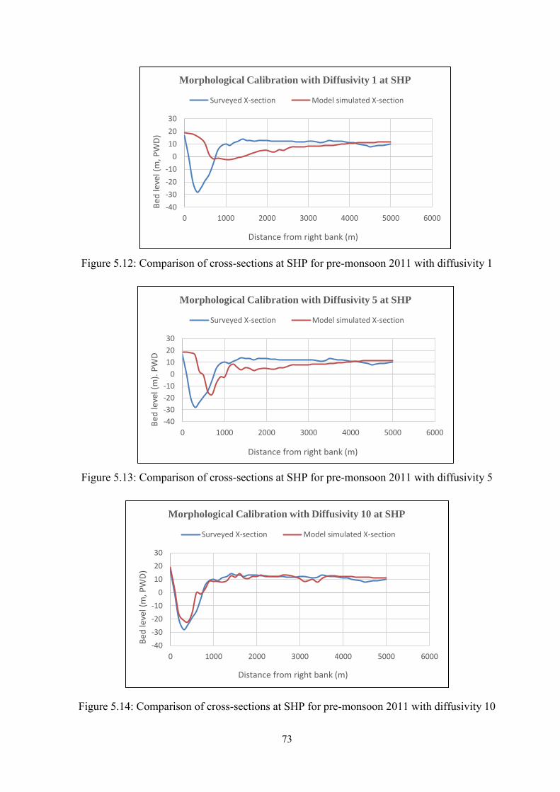
73
Figure 5.12: Comparison of cross-sections at SHP for pre-monsoon 2011 with diffusivity 1
Figure 5.13: Comparison of cross-sections at SHP for pre-monsoon 2011 with diffusivity 5
Figure 5.14: Comparison of cross-sections at SHP for pre-monsoon 2011 with diffusivity 10
-40
-30
-20
-10
0
10
20
30
0 1000 2000 3000 4000 5000 6000
Bed
leve
l (m
, PW
D)
Distance from right bank (m)
Morphological Calibration with Diffusivity 1 at SHP
Surveyed X-section Model simulated X-section
-40
-30
-20
-10
0
10
20
30
0 1000 2000 3000 4000 5000 6000
Bed
leve
l (m
). P
WD
Distance from right bank (m)
Morphological Calibration with Diffusivity 5 at SHP
Surveyed X-section Model simulated X-section
-40
-30
-20
-10
0
10
20
30
0 1000 2000 3000 4000 5000 6000
Bed
leve
l (m
, PW
D)
Distance from right bank (m)
Morphological Calibration with Diffusivity 10 at SHP
Surveyed X-section Model simulated X-section

74
5.2.8 Comparison of Simulated Water Level between MIKE21C and Delft3D
This comparison is also a validation of the model output. Because MIKE21C is a professional
software which is established and many analysis in professional and commercial cases have
done using the software. Whereas the model used in this study is Delft3D open source software
used in academic purposes mostly. If the model output of the same parameter at the same time
period of this two software matches then it will be a strong validation of the Delft3D software
used in this study.
Figure 5.15: Comparison of simulated WL data between MIKE21C and Delft3D in 2012 at Sirajganj
Figure 6.29 shows the comparison between simulated water level as obtained using MIKE21C
(Haque, 2018) simulated results. The maximum variation from MIKE21C in this case is 7.41%
which is quite acceptable. So, the validation of the Delft3D is done again comparing the result
with the established professional software MIKE21C.
0
2
4
6
8
10
12
14
16
20-May 9-Jun 29-Jun 19-Jul 8-Aug 28-Aug 17-Sep 7-Oct
WL,
mP
WD
Date
Comparison of simulated WL data between MIKE21C and
Delft3D in 2012 at Sirajganj
MIKE21C Delft3D

75
5.2.9 Model Stability Analysis
Stability analysis of a model is a prerequisite now a days when working with such type of
tools. In this case the fine grid has been taken as m = 152 and n = 752 and the total number of
grid is 114304. Then for stability analysis, a coarser grid has been taken where the number of
grid in m and n directions are half of the previous. Here m = 77, n = 377 and the total number
of grid is 29029 which is almost one-fourth of the previous total grid. After simulation with
the coarser grid with different time steps the results are as follows in Table 5.2.
Table 5.2: Stability analysis results of the model
Grid
type
Grid
size
(m×n)
No. of
grid
points
Stability
Hydrodynamic Morphologic
Time step Time step
1 min 5 min 10 min 1 min 5 min 10 min
Coarser 77×377 29029 Stable Stable Unstable Stable Unstable Unstable
Finer 152×752 114304 Stable Unstable Unstable Stable Unstable Unstable
From the stability analysis results, it has been found that in this range of the grid size the model
is stable but time step dependent. In case of time step variation the model becomes unstable
sometimes. In case of stability analysis, the calibration curves at different points show closer
result with the observed data. And the non-stable time steps show almost same results in the
model output. The Figure 5.10 shows the calibration curve for stability analysis for coarse
grid.
5.3 Model Simulation with Different Options
This study mainly deals with the structural intervention as like groyne or spurs in the erosion
prone areas of the right bank of the Jamuna River. So, different number of groynes with
different spacing will be inserted into the river to observe the hydro-morphological changes
over the year and for future prediction. The length of the groyne normally is about (25-30)%
of the average width of the river (Dani et al., 2013). However in this study, groyne length has
been assumed as one-fourth of the corresponding channel. Considering the average width of
the channel, the length of the groynes ranges from 800 m to 1000 m. The erosion prone areas
of the reach is shown in Figure 5.8 which has been collected from BWDB.

76
Figure 5.16: Erosion prone areas at the right bank of the Jamuna River
(Source: BWDB)
Different types of structures have already been constructed in the Jamuna River and among
them a number of groynes were also but in most of the cases they were washed out or damaged.
In the recent years BWDB has again constructed some cross bars at the right bank of the
Jamuna. So, the study interest is here that the number and spacing of groynes might have some
influences not to be reached in such vulnerable situation. Because the previously constructed

77
groynes were single or somewhere multiple but the series of groynes with different spacing
has not been experimented more in the BRE. So in this study the comparison among the base
situation, single groynes and series of groynes with different spacing has been done. Material
concern of the groynes has not been considered only impermeable perpendicular type
structures have been inserted to conduct this study. Because the objective of this study was to
observe the change in the hydrodynamic and morphologic parameter due to the groynes
insertion at BRE at different numbers with different spacing.
The groynes have been inserted at the upstream of the Sirajganj hard point. The locations of
the structures are between Simla and Subhagacha. The chainage range is almost BRE km 150
to 158. The shape of the groynes are normal/perpendicular. From the study of (Dani et al.,
2013) it was found that groynes with a perpendicular orientation to the oncoming flow were
optimal. So the shape of the structures were at right angled to the BRE.
Now the different options of the structural intervention are described as follows in Table 5.3.
Table 5.3: Description of the simulation options
Name of the options Description of the options
Base Without any structure
Option 1 With single groyne
Option 2 With 2 groynes with S/L ration 1.0
Option 3 With 2 groynes with S/L ration 1.5
Option 4 With 2 groynes with S/L ration 2.0
Option 5 With 3 groynes with S/L ration 1.0
Option 6 With 3 groynes with S/L ration 1.5
Option 7 With 3 groynes with S/L ration 2.0

78
Now the options for the structural intervention are shown in figures.
Figure 5.17: Base (without any structure)
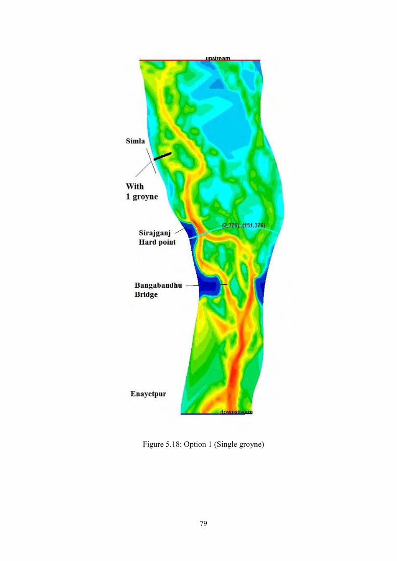
79
Figure 5.18: Option 1 (Single groyne)

80
Figure 5.19: Option 2 (2 groynes with S/L ratio 1.0)

81
Figure 5.20: Option 3 (2 groynes with S/L ratio 1.5)

82
Figure 5.21: Option 4 (2 groyne with S/L ratio 2.0)

83
Figure 5.22: Option 5 (3 groyne with S/L ratio 1.0)

84
Figure 5.23: Option 6 (3 groyne with S/L ratio 1.5)

85
Figure 5.24: Option 7 (3 groyne with S/L ratio 2.0)
All the mentioned cases have been simulated and the response of the corresponding river has
been observed. Water level, depth averaged velocity, bed shear stress, erosion/deposition,
suspended sediment transportation etc. has been observed and change in the morphology has
also been detected.

86
CHAPTER 6
RESULTS AND DISCUSSIONS
6.1 General
To understand the river response due to structural intervention, the option simulations has been
compared with the base condition and also be compared with each other. The hydrodynamic
and morphologic parameters are compared and then the relationship between/among them is
established. Different cases of the results are shown with figures in the next sections with
necessary discussions.
6.2 Observation of Hydrodynamic Parameters
Some sample figures showing the hydrodynamic parameters like, water level, depth averaged
velocity, bed shear stress etc. are displayed sequentially to observe the scenarios.
Figure 6.1: Water level at different dates for 2 groynes with S/L = 1.5

87
Figure 6.2: Depth averaged velocities at different dates for 2 groynes with S/L = 1.5
Figure 6.3: Bed shear stress at different dates for 2 groynes with S/L = 1.5
The figures mentioned above are the map files of the model output. Now the change in the
hydrodynamic parameters with their numerical values has been observed. To do this 4
observation points have been chosen. The points are:
Upstream of the structure: noted as U/S
Downstream of the structure: noted as D/S
Sirajganj Hard Point: noted as SHP
Bangabandhu Bridge Site: noted as BBS

88
6.2.1 Velocity Vectors
After simulation all the models, the output are taken from the QUICKPLOT option. Here the
direction of the velocities are shown for all the cases. As the whole area is large and the vectors
are not visible finding the large area, the vectors are shown at the selected small area. The
following figures shows the velocity vectors for all the options with the base. From the Figure
6.4, it is observed that due to the insertion of groynes, the direction of flow is diverted away
from the bank thus makes the bank free from danger. From the analysis of velocity vectors, it
is found that with the increasing number of groyne, the direction of the flow velocity moves
away from the river bank. If the spacing is large, the intermediate vectors form curvilinear
concave shapes. Another scenario is if the spacing of the groynes is increased, the flow slightly
enters into the space between two groynes. Analyzing all the figures in this case, it can be
supposed that if the S/L ratio is further increased (S/L > 2.0) then the flow reaches the bank
making it vulnerable for erosion.

89
(a) (b)

90
(c) (d)

91
(e) (f)

92
(g) (h)
Figure 6.4: Velocity vectors from model output for (a) Base, (b) Option 1, (c) Option 2, (d) Option 3, (e) option 4, (f) Option 5, (g) Option 6 and (h) Option 7

93
6.2.2 Depth Averaged Velocity
The depth averaged velocity at the upstream and downstream locations reduces as the number
of groynes increase. It is obvious that any obstacle reduces the velocity of any fluid. As the
groynes are permanent obstacles so at the upstream the velocity reduces. The velocity vectors
change their moving directions from the nose of the groynes thus at the downstream point less
water can enter with low velocity. So the curves for upstream and downstream show
reasonable results. But at SHP and at the BBS the values don’t show much fluctuations. This
may be due to the long distance between the locations or may be due to the effect of
Bangabandhu Bridge or any other reasons because Braided River like the Jamuna is the most
unpredictable in behavior. From the velocity map file, it is also observed that the near bank
velocity decreases when more structures are inserted into the river. The direction of velocity
is described in the velocity vector section (6.2.1). From that section, it is seen that the direction
of velocity has been changed after introducing the structures. That’s why the magnitude of the
velocity near the bank reaches to almost zero sometimes.
Now, the variation of depth averaged velocity with different option at a specific location will
be shown. Here, the velocities have been compared option wise with the base condition. The
Figure 6.5 and Figure 6.6 express that the due to the insertion of groyne(s), the velocity
decreases significantly at the upstream and downstream locations of the structure(s).
Consequently at SHP and BBS, there are no significant effect(s) of the structure(s) on velocity
with compared to the previous locations (Figure 6.7 and Figure 6.8).
Thus, it can be accomplished that the number of groynes affects the direction and magnitude
of the depth averaged velocity basically at the surrounding portions of the structures. Here
from the results at the upstream, the changing trend is always decreasing and the maximum
depletion of velocity from base is 0.5 m/s for the option 7. In case of downstream, the trend
shows some fluctuating behavior up to option 4 but after that for the options 5, 6 and 7 the
velocity decreases significantly and the maximum reduction in velocity is 0.9 m/s for the
option 7 compared to the base condition. The difference is more for the last three options may
be due to the backwater effect of the small sand bar situated immediately downstream of the
3rd groyne. So, it can be supposed that the more the number of groynes, the less the magnitude
in velocity. It is obvious that with the increasing number of obstacles in the way of any fluid
flow, the speed might reduce. So, in this particular case for velocity the analysis shows
reasonable output indicating that the river bank is safer when the number of groynes is more.

94
Figure 6.5: Relative comparison of velocity variation at groyne u/s for different options
Figure 6.6: Relative comparison of velocity variation at groyne d/s for different options
0
0.2
0.4
0.6
0.8
1
1.2
1.4
1.6
1.8
2
11-May 31-May 20-Jun 10-Jul 30-Jul 19-Aug 8-Sep 28-Sep 18-Oct
Vel
ocity
(m/s
)
Date
Velocity variation at u/s location of 1st groyne for different options
Base
Option 1
Option 2
Option 3
Option 4
Option 5
Option 6
Option 7
0
0.2
0.4
0.6
0.8
1
1.2
1.4
1.6
1.8
2
11-May 31-May 20-Jun 10-Jul 30-Jul 19-Aug 8-Sep 28-Sep 18-Oct
Vel
ocity
(m/s
)
Date
Velocity variation at d/s point of last groyne for different options
Base
Option 1
Option 2
Option 3
Option 4
Option 5
Option 6
Option 7

95
Figure 6.7: Relative comparison of velocity variation at groyne SHP for different options
Figure 6.8: Relative comparison of velocity variation at groyne BBS for different options
0
0.5
1
1.5
2
2.5
3
3.5
4
11-May 31-May 20-Jun 10-Jul 30-Jul 19-Aug 8-Sep 28-Sep 18-Oct
Vel
ocity
(m/s
)
Date
Velocity variation at SHP for different options
Base
Option 1
Option 2
Option 3
Option 4
Option 5
Option 6
Option 7
0
0.5
1
1.5
2
2.5
3
3.5
11-May 31-May 20-Jun 10-Jul 30-Jul 19-Aug 8-Sep 28-Sep 18-Oct
Vel
ocity
(m/s
)
Date
Velocity variation at BBS for different options
Base
Option 1
Option 2
Option 3
Option 4
Option 5
Option 6
Option 7

96
Some other figures are shown below expressing the specific comparison of the velocity at the
upstream and downstream locations of each groyne. At first the Figure 6.9 shows the variation
of line velocity immediately upstream of the 1st groyne with respect to base condition. Here,
up to the groyne length the velocity decreases significantly and the maximum reduction in
velocity is 75%. After crossing the nose of the groyne, a little bit increment of velocity has
been noticed (maximum 25%). The effect of groyne extends up to 1 km from the nose.
Figure 6.9: Comparison of velocity with base at the u/s of 1st groyne for option 2
Figure 6.10: Comparison of velocity with base at the d/s of 1st groyne for option 2
0
0.5
1
1.5
2
2.5
0 500 1000 1500 2000 2500 3000 3500 4000
Vel
ocity
(m/s
)
Distance from right bank (m)
Velocity variation with respect to base at u/s of 1st groyne
Base 1st groyne u/s Nose of groyne
0
0.5
1
1.5
2
2.5
0 500 1000 1500 2000 2500 3000 3500 4000
Vel
ocity
(m/s
)
Distance from right bank (m)
Velocity variation with respect to base at d/s of 1st groyne
Base 1st groyne d/s Nose of groyne

97
Figure 6.10 shows the variation of line velocity immediately downstream of the 1st groyne
with respect to base condition. Here, up to the groyne length the velocity decreases
considerably and the maximum reduction in velocity is more than 90%. After crossing the
nose of the groyne, a little bit increment of velocity has been noticed (maximum 25%). The
effect of groyne extends up to 1 km from the nose which is similar to the previous case.
Figure 6.11: Comparison of velocity with base at the u/s of 2nd groyne for option 2
Figure 6.11 and 6.12 show the variation of line velocity immediately upstream and downstream of the 2nd groyne with respect to base condition respectively. For these two cases, variation pattern is almost similar to the Figure 6.10 without some increasing values of velocities up to the groyne length from the bank. The effect of groyne in to the river for all cases show more or less same value which is 1 km from the nose of the groyne.
Figure 6.12: Comparison of velocity with base at the d/s of 2nd groyne for option 2
0
0.5
1
1.5
2
2.5
0 500 1000 1500 2000 2500 3000 3500 4000
Vel
ocity
(m/s
)
Distance from right bank (m)
Velocity variation with respect to base at u/s of 2nd groyne
Base 2nd groyne u/s Nose of groyne
0
0.5
1
1.5
2
2.5
0 500 1000 1500 2000 2500 3000 3500 4000
Vel
ocity
(m/s
)
Distance from right bank (m)
Velocity variation with respect to base at d/s of 2nd groyne
Base 2nd groyne d/s Nose of groyne

98
6.2.2.1 Bank Line Velocity
In this section, comparison of bank line velocities among different groyne spacing are
presented. This velocities have been observed along the line near the bank between two
consecutive groynes (Figure 6.13). From the observation, it is found that at the base condition
the velocities range 0.54 m/s to 0.62 m/s which is considerable higher than the critical value.
Because the average grain size of the river is 0.11 mm and for this grain size, the critical
velocity is 0.20 m/s (20 cm/sec) according to Hjulstrӧms diagram (Figure 4.7). So, the river
bank is susceptible to erosion at normal condition. Also the BWDB has identified this bank as
erosion prone area (Figure 5.16). Now for the spacing ratio of the groyne, S/L = 1.0, the
velocity decreases significantly and belongs to less than or equal to 0.1 m/s. With the
increasing option, the magnitude of velocities increase and up to S/L = 2.0, the velocity is far
from the critical value. But after that the value reaches and crosses the critical velocity line for
S/L = 3.0 and if this pattern continues, the more spacing option will increase the velocity as
well and reach up to the base condition. So, it is risky in this case, to provide spacing ration
more than 2.0. Although the spacing ratio 2.5 may remain below the critical line.
Figure 6.13: Comparison of bank line velocities for different spacing of groynes
0
0.1
0.2
0.3
0.4
0.5
0.6
0.7
35500 36000 36500 37000 37500
Vel
ocity
(m/s
)
Distance from downstream boundary (m)
Variation of bank line velocity with different groyne spacing
Base
S/L=1.0
S/L=1.5
S/L=2.0
S/L=3.0
Critical line

99
6.2.3 Bed Shear Stress
Bed shear stress is the result of drag force. If the velocity of water decreases, simultaneously
the magnitude of the drag force will be reduced. That’s why the variation of bed shear stress
basically follows the velocity variation. From the model output it is observed that at the
upstream and downstream locations, the value of bed shear stress decrease significantly with
increasing the options (Figure 6.15 and Figure 6.16) and no such effects at SHP and BBS
locations (Figure 6.17 and Figure 6.18)
Figure 6.14: Relative comparison of bed shear stress at groyne u/s for different options
Figure 6.15: Relative comparison of bed shear stress at groyne d/s for different options
0
1
2
3
4
5
6
11-May 31-May 20-Jun 10-Jul 30-Jul 19-Aug 8-Sep 28-Sep 18-Oct
Bed
shea
r stre
ss (N
/m2)
Date
Bed shear stress variation at u/s point for different options
Base
Option 1
Option 2
Option 3
Option 4
Option 5
Option 6
Option 7
0
0.5
1
1.5
2
2.5
3
3.5
4
4.5
5
11-May 31-May 20-Jun 10-Jul 30-Jul 19-Aug 8-Sep 28-Sep 18-Oct
Bed
shea
r stre
ss (N
/m2)
Date
Bed shear stress variation at d/s point for different options
Base
Option 1
Option 2
Option 3
Option 4
Option 5
Option 6
Option 7

100
Figure 6.16: Relative comparison of bed shear stress at groyne SHP for different options
Figure 6.17: Relative comparison of bed shear stress at groyne BBS for different options
0
2
4
6
8
10
12
14
11-May 31-May 20-Jun 10-Jul 30-Jul 19-Aug 8-Sep 28-Sep 18-Oct
Bed
shea
r stre
ss (N
/m2)
Date
Bed shear stress variation at SHP for different options
Base
Option 1
Option 2
Option 3
Option 4
Option 5
Option 6
Option 7
0
2
4
6
8
10
12
14
16
11-May 31-May 20-Jun 10-Jul 30-Jul 19-Aug 8-Sep 28-Sep 18-Oct
Bed
shea
r stre
ss (N
/m2)
Date
Bed shear stress variation at BBS for different options
Base
Option 1
Option 2
Option 3
Option 4
Option 5
Option 6
Option 7

101
6.2.3.1 Bank Line Bed Shear Stress
As like the variation of velocity along the bank line, the bed shear stress variation near the
bank has also been observed. This bed shear stresses have been observed along the line near
the bank between two consecutive groynes (Figure 6.19). From the observation, it is found
that at the base condition the value of bed shear stress ranges from 0.75 N/m2 to 1.00 N/m2
which is considerable higher than the critical value. Because the average grain size of the river
is 0.11 mm and for this grain size, the critical bed shear stress is 0.14 N/m2 according to
Fischenich formula (Equation 4.1). So, the river bank is susceptible to erosion at normal
condition. Also the BWDB has identified this bank as erosion prone area (Figure 5.16). Now
for the spacing ratio of the groyne, S/L = 1.0, the bed shear stress decreases significantly and
belongs to almost zero in some places with a maximum value of 0.025 N/m2. With the
increasing option, the magnitude of bed shear stress increases and for S/L = 2.0, the bed shear
stress line is far below from the critical value. But after that the value reaches and crosses the
critical line for bed shear stress for S/L = 3.0 and if this pattern continues, the more spacing
option will increase the bed shear stress as well and reach up to the base condition. So, it is
risky in this case, to provide spacing ration more than 2.0. Although the spacing ratio 2.5 may
remain below the critical line.
Figure 6.18: Comparison of bed shear stress along the bank line for different spacing of groynes
0
0.2
0.4
0.6
0.8
1
1.2
35500 36000 36500 37000 37500
Bed
shea
r stre
ss (N
/m2)
Distance from upstream boundary (m)
Variation of bed shear stress near bank with groyne spacing
Base
S/L=1.0
S/L=2.0
S/L=3.0
Critical line

102
6.3 Observation of Morphologic parameters
Some sample figures showing the morphologic parameters like total transport, cumulative
erosion/sedimentation, cross sections etc. are displayed sequentially to observe the scenarios.
Figure 6.19: Cum. erosion/sedimentation at different dates for 2 groynes with S/L = 1.5
Figure 6.20: Total transport at different dates for 2 groynes with S/L = 1.5

103
6.3.1 Cumulative Erosion/Deposition Curves
From the cumulative erosion/deposition curves at different point for different options it is
observed that at the upstream and downstream of the structures, mostly deposition occur after
intervention although sometimes it shows erosion. But in case of SHP, there is very little effect
of the structures on erosion/deposition. The variation of the sediment at this point is almost
zero. This may be due to the distance of the SHP from the intervention point(s). Because the
SHP is located at about 8-10 km downstream of the structural intervention point. So the
structures has significant role in the vicinity only, not at far upstream or downstream points.
Another reason may be due to the problem in model simulation. Because sediment transport
is one of the most unpredictable parameters in river analysis. The mathematical model analysis
might not always match with the real scenarios. So, there may be a fault of this software of
not tracing any movement of sediment at SHP. In case of BBS, the results shows some
variation for the months August and September. This deviation might be caused due to the
backwater effect of the Bangabandhu Bridge. As the location of the BBS is far downstream,
so the effect of these structures on sediment movement has a little quantity.
Option wise cumulative erosion/deposition at specific locations have been plotted and shown
in Figure 6.23 to Figure 6.26. The graphs show that the cumulative erosion/deposition has
fluctuating behavior from the base condition at maximum points. At SHP, there is very little
variation in erosion/deposition. This may be due to the unpredictability of the Jamuna River
or this sediment model might have some inefficiencies at that point.

104
Figure 6.21: Relative comparison of cum. erosion/deposition at groyne u/s for different
options
Figure 6.22: Relative comparison of cum. erosion/deposition at groyne d/s for different
options
-3
-2
-1
0
1
2
3
4
11-May 31-May 20-Jun 10-Jul 30-Jul 19-Aug 8-Sep 28-Sep 18-Oct
Cum
. ero
sion
/sed
imen
tatio
n (m
)
Date
Cum. erosion/sedimentation at u/s point of 1st groyne for different options
Base
Option 1
Option 2
Option 3
Option 4
Option 5
Option 6
Option 7
-1.5
-1
-0.5
0
0.5
1
1.5
2
2.5
3
3.5
11-May 31-May 20-Jun 10-Jul 30-Jul 19-Aug 8-Sep 28-Sep 18-Oct
Cum
. ero
sion
/sed
imen
tatio
n (m
)
Date
Cum. erosion/sedimentation at d/s point of last groyne for different options
Base
Option 1
Option 2
Option 3
Option 4
Option 5
Option 6
Option 7

105
Figure 6.23: Relative comparison of cum. erosion/deposition at groyne SHP for different
options
Figure 6.24: Relative comparison of cum. erosion/deposition at groyne BBS for different
options
-6
-5
-4
-3
-2
-1
0
11-May 31-May 20-Jun 10-Jul 30-Jul 19-Aug 8-Sep 28-Sep 18-Oct
Cum
. ero
sion
/sed
imen
tatio
n (m
)
Date
Cum. erosion/sedimentation at u/s point for different options
Base
Option 1
Option 2
Option 3
Option 4
Option 5
Option 6
Option 7
-6
-5
-4
-3
-2
-1
0
1
11-May 31-May 20-Jun 10-Jul 30-Jul 19-Aug 8-Sep 28-Sep 18-Oct
Cum
. ero
sion
/sed
imen
tatio
n (m
)
Date
Cum. erosion/sedimentation at BBS for different options
Base
Option 1
Option 2
Option 3
Option 4
Option 5
Option 6
Option 7

106
6.3.2 Bed Level Variation at Different Locations
From the previous section the relative variation of cumulative erosion or sedimentation has
been observed at four points of interests. Now in this section, the actual bed level variation
with respect to base condition at some locations for option 2 has been shown in Figure 6.25.
One is along the length of the 1st and 2nd groyne from the right bank up to about 4 km inside
the river. These sections are denoted by a-a and c-c. Cross-section of same category at the
middle of the two consecutive groynes are denoted by b-b. Another section has been chosen
along the river in front of the noses of the groynes which is section 1-1.
Figure 6.25: Cross-section locations to observe bed level variation across and along the river for option 2

107
Option 4 Option 6
Figure 6.26: Cross-section locations to observe bed level variation across and along the river for option 4 and 6
Some another sections has been shown for option 4 and option 6 in Figure 6.26. For option 4,
the cross section is a-a and long section is 1-1. For option 6, the cross section is a-a and the
long sections are 1-1 and 2-2 respectively.

108
6.3.2.1 Bed Level Variation across the River for Option 2
To observe the bed level variation across the river for section a-a, the Figure 6.27 shows the
variation of the bed level along the 1st groyne length from the right bank of the river and
extends up to almost 4 km inside the river. From this figure, it is seen that there is major
erosion takes place just immediately after the nose of the groyne and after some distances
(around 500 m) some deposition occurs. The maximum erosion in this case is -5.25 m which
takes place immediately after the nose and maximum deposition is +3.70 m which is located
700 m from the nose. In case of section c-c, shown in Figure 6.28 the result pattern is almost
same but the values are different. Here, the maximum erosion is -4.50 m and maximum
deposition is +0.74 m.
Comparing these two figures, it can be decided that the erosion/deposition effect is more at
the 1st groyne with compared to the 2nd one. Because the value of both erosion and deposition
for the 2nd case is lower than the 1st case. Another observation is that for the both cases, the
effect of groyne withstands up to 1 km from the nose of the groyne in to the river.
Figure 6.27: Bed level variation along the 1st groyne with respect to base for option 2 (Section a-a)
0
2
4
6
8
10
12
14
16
18
0 500 1000 1500 2000 2500 3000 3500 4000
Elev
atio
n (m
, PW
D)
Distance from right bank (m)
Bed level variation along the groyne with respect to base
Base 1st groyne Groyne nose

109
Figure 6.28: Bed level variation along the 2nd groyne with respect to base for option 2 (Section c-c)
At the middle portion between the consecutive two groynes, the effect of groynes are exposed
in Figure 6.29. The comparison has been made with respect to base condition and the cross-
section extends from the right bank of the river up to around 4 km inside the river.
Figure 6.29: Bed level variation between the 1st and 2nd groyne with respect to base for option 2, option 3 and option 4 (Section b-b)
0
2
4
6
8
10
12
14
16
0 500 1000 1500 2000 2500 3000 3500 4000
Elev
atio
n (m
, PW
D)
Distance from right bank (m)
Bed level variation along the groyne with respect to base
Base 2nd groyne Groyne nose
-14
-12
-10
-8
-6
-4
-2
0
0 500 1000 1500 2000 2500 3000 3500 4000
Elev
atio
n (m
, PW
D)
Distance from right bank (m)
Bed level variation between two groynes with respect to base condition
Base
S/L=1.0
S/L=1.5
S/L=2.0

110
In this case, the comparison has been done for S/L=1.0, 1.5 and 2.0 respectively with the base.
From the figure it is noticed that major deposition takes place at two locations, one is about
1200 m from the bank the value of which is +2.37 m and another is about 1800 m from the
bank and its value is +4.5 m. Maximum erosion takes place at about 2200 m from the bank
and the value of erosion is -3.24 m. Here, the noticeable fact is that the variation of bed level
among the spacing options is very little. The pattern of this graph is somewhat similar to the
previous two cases.
6.3.2.2 Bed Level Variation along the River for Option 2
In case of observing the bed level variation along the river for section 1-1, the Figure 6.30
shows the variation of the bed level along the line extends from 34 km from the downstream
boundary up to around 40 km to the north. The line is located in front of the noses of the
groynes. Here the groyne spacing is 1.0. From the figure, it is observed that there is huge
erosion at the 1st groyne location and surrounding areas and the amount of erosion decreases
in case of 2nd groyne with different pattern. And deposition takes place at the downstream of
the 2nd groyne. No deposition is in between the two noses of the groynes. The effect of these
groynes extends up to 2 km laterally from the nose for both the cases.
Figure 6.30: Bed level variation along the river in front of the nose of the groynes with respect to base for Option 2 (S/L = 1.0) (Section 1-1)
0
1
2
3
4
5
6
7
8
9
10
34000 35000 36000 37000 38000 39000 40000
Bed
ele
vatio
n (m
, PW
D)
Distance from downstream boundary (m)
Bed level variation infront of groyne noses along the river for S/L=1.0
Base
S/L=1.0
Groyne 1
Groyne 2

111
Figure 6.31 is for the same section (Section 1-1) but for different option. Here the S/L ratio is
2.0. From the figure, it is observed that the erosion pattern is almost same at the location of
the two groynes with varying values. But the noticeable thing is that the major deposition zone
lies between the two groynes which is different from the previous case. A small deposition
zone is noticed at the downstream of the 2nd groyne. Here also the effect of these groynes
extends up to 2 km laterally from the nose for both the cases.
After comparison of these two graphs, it can be concluded that in case of smaller spacing,
there is no deposition between the groyne noses and the major deposition takes place at the
downstream of the last groyne. In case of increasing the spacing the deposition zone shifts
towards the intermediate locations between the groynes and the erosion zone at the
downstream of the last groyne comes to smaller with decreasing deposition values.
Figure 6.31: Bed level variation along the river in front of the nose of the groynes with respect to base for Option 4 (S/L=2.0) (Section 1-1)
0
1
2
3
4
5
6
7
8
9
10
32500 33500 34500 35500 36500 37500 38500 39500
Bed
ele
vatio
n (m
, PW
D)
Distance from downstream boundary (m)
Bed level variation infront of groyne noses along the river for S/L=2.0
Base
Option 4
Groyne 1
Groyne 2

112
6.3.2.3 Bed Level Variation across the River for Option 4 and Option 6
From the Figure 6.32 and Figure 6.33, it has been observed that mainly deposition takes place
between the two groynes for each cases (i.e. section a-a for option 4 and option 6) which is
relevant with results of previous several studies. The comparison has been done with respect
to base condition across the river.
Figure 6.32: Bed level variation between the 1st and 2nd groyne with respect to base for option 4 (Section a-a)
Figure 6.33: Bed level variation between the 2nd and 3rd groyne with respect to base for option 6 (Section a-a)
0
2
4
6
8
10
12
14
16
0 500 1000 1500
Bed
ele
vatio
n (m
, PW
D)
Distance from right bank (m)
Bed Level variation between two groynes for option 4
Base Option 4
Deposition
0
2
4
6
8
10
12
14
16
0 500 1000 1500
Bed
ele
vatio
n (m
, PW
D)
Distance from right bank (m)
Bed Level variation between two groynes for option 6
Base Option 6
Deposition

113
6.3.2.4 Bed Level Variation along the River for Option 4 and Option 6
In this case, the variation of bed level has been compared with the base condition along the
river. Here, Figure 6.34 shows the variation along the line in front of the noses of the groynes
for the option 4. The major erosion takes place at the location of the 1st groyne and the value
of erosion decreases at the location of the 2nd one and deposition takes place in between the
groynes. Here, the maximum erosion is almost -6.0 m and deposition is about +4.0 m.
Figure 6.34: Bed level variation along the river in front of the nose of the groynes with respect to base for Option 4 (2 groynes with S/L = 2.0) (Section 1-1)
Figure 6.35: Bed level variation along the river along the nose of the groynes with respect to base for Option 6 (3 groynes with S/L = 1.5) (Section 1-1)
0
2
4
6
8
10
12
32500 33500 34500 35500 36500 37500 38500 39500 40500
Bed
elev
atio
n (m
, PW
D)
Distance from downstream boundary (m)
Bed Level variation infront of noses of the groynes for option 4
Base Option 4
0
2
4
6
8
10
12
33500 34500 35500 36500 37500 38500 39500
Bed
ele
vatio
n (m
, PW
D)
Distance from downstream boundary (m)
Bed Level variation along the nose of the groynes for option 6
Base Option 6
Erosion
Deposition
Deposition
Erosion

114
Figure 6.35 and Figure 6.36 shows the same circumstances in case of option 6 along the noses
of the groynes and along the line in front of the noses of the groynes respectively. For these
two cases, the erosion/deposition pattern is almost same with the previous diagrams. From
these two cases, the maximum erosion is -5.0 m and deposition is +2.0 m. The effect of the
groynes laterally extends up to about 2.0 km from the groyne which is similar to the previous
that has been explained in section 6.3.2.2.
Figure 6.36: Bed level variation along the river in front of the nose of the groynes with respect to base for Option 6 (3 groynes with S/L = 1.5) (Section 1-1)
0
2
4
6
8
10
12
14
31500 33500 35500 37500 39500 41500
Bed
ele
vatio
n (m
, PW
D)
Distance from downstream boundary (m)
Bed Level variation infront of noses of the groynes for option 6
Base Option 6
Erosion
Deposition

115
6.4 Summary of the Results
In order to quantify the response of the river hydrodynamics and morphology for
various options at different locations, at first the model has been set up then calibrated
and validated subsequently for the both cases (hydrodynamics and morphology). An
attempt has been made to compare the results of water level obtained from Delft3D
with those of MIKE21C and found satisfactory. Here in this section, model results for
the month of July can be assessed as shown in Table 6.1.The remaining results can be
seen in Appendix-C. It can be seen from the results that the Jamnua River shows
reasonable responses due to the structural intervention at the right bank of the river.
As for example, at upstream of the selected intervention, water level increases about
10.84% and 6.72% for the downstream (Table 6.1, 6.2). This rise of water level may
be due to the afflux effect due to the structural intervention(s). The velocity and bed
shear stress follow decreasing trend lines at the vicinity of the structures. Similarly the
other parameters like velocity, bed shear stress and cumulative erosion/deposition
show considerable responses for the selected intervention (options). The changes are
+9.92% for velocity, +22.78% for bed shear stress and no erosion/deposition are
obtained. At Bangabandu Bridge site (Table 6.4), the water level doesn’t change but
the velocity follows decreasing trends.
From the velocity vector diagrams, it is observed that the direction of velocity changes
and diverted away from the bank with the structural intervention. If the spacing
between the groynes increases the vectors enters into the intermediate potions between
the groynes forming a curvature shape. And from the bank line velocity and bed shear
stress analysis, it is clear that for this reach of the river the spacing ratio more than 2.0
is dangerous because in case of spacing ratio 3.0, the bank line velocity and bed shear
stress both cross the critical line.
In case of bed level variation, erosion takes place along the length of the groyne
basically in front of nose and deposition occurs more or less 500 m front side of the
nose of the groyne. The variation of the middle portion between the groynes shows the
similar pattern. In case of lateral variation along the river in front of the groyne nose,
the deposition zone shifts towards the intermediate locations between the groynes from
the downstream. The effect of groyne extends up to 1 km inside the river and 2 km

116
laterally from either nose of the groyne.
Thus it can be supposed that to prevent the bank erosion, this kinds of structures with
increasing numbers and different spacing provides satisfactory results. Overall, the
model results show that it has the capacity to assess responses for various options at
the vicinity of the interventions.
Table 6.1: Change of parameters with respect to base condition at u/s for various options (July)
Upstream of structure
Options WL (%)
Velocity (%)
Bed shear stress (%)
Erosion/deposition (m)
1 groyne 8.16 -39.78 -60.86 1.54 2 groynes with S/L=1.0 9.32 -46.41 -69.85 -1.16 2 groynes with S/L=1.5 8.53 -30.94 -33.33 3.41 2 groynes with S/L=2.0 9.39 -64.09 -88.76 -4.62 3 groynes with S/L=1.0 8.89 -31.49 -32.40 4.13 3 groynes with S/L=1.5 9.32 -37.02 -50.19 3.96 3 groynes with S/L=2.0 10.84 -31.49 -49.63 -0.20
+ ve means increase/deposition, - ve means decrease/erosion
Table 6.2: Change of parameters with respect to base condition at d/s for various options (July)
Downstream of structure
Options WL (%)
Velocity (%)
Bed shear stress (%)
Erosion/deposition (m)
1 groyne 6.58 34.44 66.67 0.00 2 groynes with S/L=1.0 8.16 -16.56 -26.09 0.76 2 groynes with S/L=1.5 7.44 -74.17 -91.30 -2.29 2 groynes with S/L=2.0 6.79 11.92 14.78 -6.00 3 groynes with S/L=1.0 7.15 -84.11 -96.52 2.81 3 groynes with S/L=1.5 6.65 -5.30 -24.64 0.78 3 groynes with S/L=2.0 6.72 -45.70 -44.93 1.93
+ ve means increase/deposition, - ve means decrease/erosion

117
Table 6.3: Change of parameters with respect to base condition at SHP for various options (July)
Sirajganj Hard Point (SHP)
Ooptions WL (%)
Velocity (%)
Bed shear stress (%)
Erosion/deposition (m)
1 groyne -0.07 1.19 2.95 -5.00 2 groynes with S/L=1.0 0.00 31.35 73.84 -5.00 2 groynes with S/L=1.5 0.14 25.40 58.51 -5.00 2 groynes with S/L=2.0 0.57 13.10 33.33 -5.00 3 groynes with S/L=1.0 1.07 16.27 35.72 -5.00 3 groynes with S/L=1.5 0.93 21.03 48.52 -5.00 3 groynes with S/L=2.0 1.72 9.92 22.78 -5.00
+ ve means increase/deposition, - ve means decrease/erosion
Table 6.4: Change of parameters with respect to base condition at BBS for various options (July)
Bangabandhu Bridge Site (BBS)
options WL (%)
Velocity (%)
Bed shear stress (%)
Erosion/deposition (m)
1 groyne -0.08 -3.83 23.74 -6.00 2 groynes with S/L=1.0 -0.85 -23.96 51.95 6.70 2 groynes with S/L=1.5 -0.85 -67.73 -69.84 5.15 2 groynes with S/L=2.0 -0.08 -24.28 -7.98 -2.10 3 groynes with S/L=1.0 -1.00 -62.94 -50.00 5.90 3 groynes with S/L=1.5 0.15 -37.38 -20.53 2.92 3 groynes with S/L=2.0 0.00 -6.07 28.02 -6.00
+ ve means increase/deposition, - ve means decrease/erosion

118
Table 6.5: Monthly variation of cum. erosion/deposition at different locations for all the options
Cum. Erosion/Deposition (m)
u/s
Date Base Option 1 Option 2 Option 3 Option 4 Option 5 Option 6 Option 7
1-Jun -0.12279 0.001034 -0.05414 -0.06206 -0.06963 0.838351 9.54E-06 -0.21957
1-Jul -3.38927 1.73075 -1.15469 3.40705 -4.82042 -4.82339 3.27664 -0.20424
1-Aug -4.99852 1.8153 -1.01404 1.1501 3.2922 2.44095 3.27664 -0.31912
1-Sep 3.14144 4.52101 -4.99971 -4.98486 -4.99994 1.97879 3.27662 -0.28024
30-Sep -4.9991 1.97102 4.45679 3.76438 3.90919 0.936223 3.27696 -4.99526
d/s
Date Base Option 1 Option 2 Option 3 Option 4 Option 5 Option 6 Option 7
1-Jun -0.07394 9.54E-07 0.052472 0 9.63E-05 0 0 0
1-Jul -2.23368 0.00847 0.756154 -0.33232 -4.99733 2.67702 2.46979 1.92763
1-Aug -1.60298 0.023461 0.820639 2.91779 -5 4.10148 4.14746 0.086869
1-Sep 7.19262 -0.52265 -4.88794 3.44129 -1.74733 5.44723 4.16025 0.356354
30-Sep 5.46633 -0.5785 -4.99955 5.08437 -4.99998 -2.18086 5.55232 2.20797
SHP
Date Base Option 1 Option 2 Option 3 Option 4 Option 5 Option 6 Option 7 1-Jun -0.82777 -0.82621 -0.85794 -0.85684 -0.85942 -0.85865 -0.85592 -0.85893
1-Jul -5 -5 -5 -5 -5 -5 -5 -5
1-Aug -5 -5 -2.85595 -2.85853 -2.85589 -5 -5 -2.85065
1-Sep -5 -5 -5 -5 -5 -2.22311 -5 -5
30-Sep -5 -5 -5 -5 -5 -5 -5 -5
BBS
Date Base Option 1 Option 2 Option 3 Option 4 Option 5 Option 6 Option 7
1-Jun 0.696684 0.696303 0.785183 0.786232 0.7864 0.785315 0.785878 0.786103
1-Jul 4.57916 -4.99679 5.29778 5.15313 -2.09781 5.90294 2.9223 -4.99731
1-Aug 6.67965 -4.99956 -5 6.69503 -5 -5 0.221426 1.50671
1-Sep 5.57396 -4.99916 5.83188 2.64203 5.68807 -5 3.4995 5.65976
30-Sep 3.98544 -4.99925 0.626596 1.60514 1.59909 6.77034 7.61095 -2.71065

119
CHAPTER 7
CONCLUSIONS AND RECOMMEDATIONS
7.1 General
Assessment of river responses for any structural intervention in the braided river like Jamuna
River is a complex task. Two-dimensional morphological model has become a useful tool for
analyzing the hydrodynamic and morphological behavior of such river. In this study, efforts
have been given to assess the river responses due to structural intervention.
7.2 Conclusions
The following concluding remarks can be drawn from the present study-
i. A two-dimensional mathematical model with Delft3D software has been set up for flow
with sediment transport. The model has been calibrated and validated with the reasonable
accuracy, thus this model can be available for analyzing the river responses for selected
structural intervention.
ii. Responses of the Jamuna River have been assessed from the model simulations for
different options using groyne as a structural intervention. In this study, seven different
options with groyne of number such as 1, 2 and 3 with spacing ratio 1.0, 1.5 and 2.0.
iii. Model results indicate that at upstream of the selected intervention, water level increases
about 10.84% and 6.72% for the downstream. In both cases, the reduction of velocity
and the bed shear stress is more than 50%.
iv. For observation, four points were selected among them the effects are considerable at
the upstream and downstream of the groyne(s) and for the other two points (e.g. Sirajganj
Hard Point and Bangabandhu Bridge Site) the effect is very little due to the long distance.
v. From the velocity vectors and bank line velocities as well as bed shear stress, it can be
decided that for this specific reach of the river, the maximum allowable spacing between
the groynes is 2.0 times of its length. Otherwise the bank will be in vulnerable condition
due to erosion.
vi. The bed level variation surrounding the groynes is considerable. The effect of groyne
extends up to 1 km inside the river and 2 km laterally from either nose of the groyne.
The maximum erosion is -5.25 m and deposition is +3.70 m along the length of the

120
groyne. In case of lateral section (along the river) the values are -6.0 m and +4.0 m
respectively.
vii. Selected hydrodynamic and morphologic scenarios are extracted from model then
interpreted and observed that due to structural intervention, there are significant effects
on those variables in case of the selected reach of the Jamuna River.
viii. Finally, it can be concluded that river bank erosion can be decreased by using the
increasing number of such type of transverse structures (groyne) with different spacing
and the effect of these types of structures have more influences at the vicinity.
7.3 Recommendations for Further Study
Based on the present study following recommendations can be made for future study-
i. As Jamuna is an alluvial river in a deltaic region of Bangladesh, so morphological
activities are very dynamic in this river. Structural intervention is only fruitful when
maintenance is regular.
ii. In this study a selected reach has been used for analysis. Therefore, effectiveness
of the results found in this study should be much better when the other reaches could be
included.
iii. In this study two-dimensional morphological model is used which gives depth
average velocity from simulations. Therefore, the prediction of local phenomena
like scour at toe level (under water) cannot be properly predicted. 3-D model would
be more helpful for such computations.
iv. Changing the groyne length simultaneously and for more options, the study may give
much better results to identify the response of the river.
v. Comparison with the physical model study is the best way of analysis in this case. So,
any mathematical model output need to be verified with the physical model output or
field data prior to implementation
vi. In this study, the structures have been incorporated only one side. Further study may be
proceeded by incorporating the structural intervention at the both banks of the river using
different options.

121
REFERENCES
Abbas, B. G., Mojtaba, G. K. (2009) ‘Effect of Groyens Opening Percentage on River Outer Bank
Protection’, Journal of Applied Sciences, 9(12), pp. 2325–2329.
Ahmad, H. F., Bhat, M. S. and Ahmad, S. (2016) ‘One Dimensional Steady Flow Analysis Using
HEC- RAS – A case of River Jhelum , Jammu and Kashmir’, European Scientific Journal, 12(32),
pp. 340–350. doi: 10.19044/esj.2016.v12n32p340.
Ahmed, T. and Hasan, M. Z. (2011) ‘A Study on River Bank Protection Works and Flooding of
Sirajganj Town’. Bangladesh University of Engineering and Technology, Bangladesh.
Alam, S. and Matin, M. A. (2012) ‘Application of Delft3D Mathematical Model in the river
Karnafuli For Two-Dimensional simulation’, in 1st International Conference on Advances in Civil
Engineering 2012 (ICACE 2012), CUET, Chittagong, Bangladesh, pp. 12–14.
Alam, S. and Matin, M. A. (2013) ‘Application of 2D morphological model to assess the response
of Karnafuli River due to capital dredging’, Journal of Water Resources and Ocean Science, 2(3),
pp. 40–48. doi: 10.11648/j.wros.20130203.13.
Alauddin, M. (2011) ‘Morphological Stabilization of Lowland Rivers by using a Series of
Groynes’. Nagoya University, Japan.
Ali, A., Mynett, a. E. and Azam, M. H. (2007) ‘Sediment Dynamics in the Meghna Estuary,
Bangladesh: A Model Study’, Journal of Waterway, Port, Coastal, and Ocean Engineering,
133(August), pp. 255–263. doi: 10.1061/(ASCE)0733-950X(2007)133:4(255).
Ali, M. M. (2004) ‘Hydrodynamic Simulation of the River Jamuna’. Bangladesh University of
Engineering and Technology, Dhaka.
Best, J. L. et al. (2003) ‘Three-Dimensional Sedimentary Architecture of a Large, Mid-Channel
Sand Braid Bar, Jamuna River, Bangladesh’, Journal of Sedimentary Research, 73(4), pp. 516–
530. doi: 10.1306/010603730516.
Best, J. L. et al. (2007) ‘The Brahmaputra-Jamuna River , Bangladesh’.
Briere, C., Giardino, A. and Van der Werf, J. (2011) ‘Morphological Modeling of Bar Dynamics
With Delft3D: the Quest for Optimal Free Parameter Settings Using an Automatic Calibration

122
Technique’, Coastal Engineering Proceedings, 1(32), p. 60. doi: 10.9753/icce.v32.sediment.60.
Churuksaeva, V. and Starchenko, A. (2015) ‘Mathematical modeling of a river stream based on a
shallow water approach, Procedia - Procedia Computer Science’. Elsevier Masson SAS. doi:
10.1016/j.procs.2015.11.024.
Coleman, J. M. (1969) ‘Brahmaputra River: channel processes and sedimentation’, Sediment.
Geol., 3(129-239).
Dani, B. A. et al. (2013) ‘An investigation of the use of groynes as a means of riverbank erosion
protection’, (March).
Dargahi, B. (2004) ‘Three-dimensional flow modelling and sediment, transport in the River
Klarälven’, Earth Surface Processes and Landforms, 29(7), pp. 821–852. doi: 10.1002/esp.1071.
Elias, E. P. L. et al. (2001) ‘Hydrodynamic Validation of Delft3D with Field Measurements at
Egmond’, Coastal Engineering 2000, pp. 2714–2727. doi: 10.1061/40549(276)212.
FAP1 (1991) ‘River Training Studies of the Brahmaputra River’.
FAP2 (1992) ‘North West Regional Study’.
FAP21/22 (2001) “Bank protection and river training (AFPM) pilot project,” Final project
evaluation report, Volume I, WARPO, Ministry of water resources, Government of People’s
Republic of Bangladesh., I, p. 2001.
FAP24 (1996) ‘Morphological processes in the Jamuna River’, Special Report No. 24, River
Survey Project, Prepared for Water Resources Planning Organization (WARPO), Dhaka,
Bangladesh.
Garg, S. K. (2005) ‘Irrigation Engineering & Hydraulic Structures’. 19th edn. Khanna Publishers.
doi: 10.15713/ins.mmj.3.
Goodell, C, Warren, C. (2006) ‘Flood Inundation Mapping using HEC-RAS’.
Haque, A. Z. M. S. (2018) ‘Hydrodynamic and Morphological Analysis of New Dhaleswari River
Offtake using Mathematical Model’. Bangladesh University of Engineering and Technology.
Hassanzadeh, Y. (2012) ‘Hydraulics of Sediment Transport’, Hydrodynamics - Theory and

123
Model, (1984). doi: 10.5772/25982.
Hjulstrӧm, F. (1935) ‘Studies of the Morphological Activity of Rivers as Illustrated by the River
Fyris’, PhD Thesis, Geological Institute Upsalsa.
Hongwei, Z., Xuehua, Z. and Bao’an, Z. (2009) ‘System Dynamics Approach to Urban Water
Demand Forecasting’, Transactions of Tianjin University, 15(1), pp. 70–74. doi: 10.1007/s12209.
Hoque Mollah, T. and Ferdaush, J. (2015) ‘Riverbank Erosion, Population Migration and Rural
Vulnerability in Bangladesh (A Case Study on Kazipur Upazila at Sirajgonj District)’,
Environment and Ecology Research, 3(5), pp. 125–131. doi: 10.13189/eer.2015.030502.
Ivanova, O. and Ivanov, M. (2016) ‘1-D Mathematical Modelling of Flood Wave Propagation’,
53, pp. 139–144. doi: 10.3303/CET1653024.
Kolmogorov, A. N. (1942) ‘Equations of turbulent motion of an incompressible fluid’, IZV Akad.
Nauk. USSR, Ser. Phys., 6, pp. 56–58.
Lesser, G. R. et al. (2004) ‘Development and validation of a three-dimensional morphological
model’, Coastal Engineering, 51(8-9), pp. 883–915. doi: 10.1016/j.coastaleng.2004.07.014.
Manual, D.-F. U. (2013) ‘Simulation of multi-dimensional hydrodynamic flows and transport
phenomena, including sediments’, 3.15.30932.
Matin, D. M. A. (2016) ‘An overview of River Bank Protection in Bangladesh’. Bangladesh
University of Engineering and Technology.
Matsuda, I. (2004) ‘River Morphology And Channel Processes’, Encyclopedia of Life Support
Systems (EOLSS), p. 12.
Morianou, G. G. et al. (2015) ‘2D Simulation of Water Depth and Flow Velocity using the MIKE
21C Model’, in, pp. 3–5.
Moriasi, D. N. et al. (2007) ‘Model Evaluation Guidelines for Systematic Quantification of
Accuracy in Watershed Simulations’, American Society of Agricultural and Biological Engineers,
50(3), pp. 885–900.
Mosselman, E. (2006) ‘Bank protection and river training along the braided Brahmaputra-Jamuna
River, Bangladesh.’, Braided Rivers: Process, deposits, ecology and management. Special

124
Publication No. 36 of the International Association of Sedimentologists., pp. 278–287. doi:
10.1002/9781444304374.ch13.
Musfequzzaman, M. (2012) ‘Study of Hydro-Morphological Impact of Dredging in Selected
Reach of the River Jamuna using Two-Dimensional Morphological Model’, MSc. Engg. Thesis,
Department of Water Resources Engineering, BUET, Dhaka, T-261(July).
Nicholas, A. P. (2013) ‘Modelling the continuum of river channel patterns’, Earth Surface
Processes and Landforms, 38(10), pp. 1187–1196. doi: 10.1002/esp.3431.
Noor, F. (2013) ‘Morphological Study of Old Brahmaputra Offtake using Two-Dimensional
Mathematical Model’. Bangladesh University of Engineering and Technology, Dhaka.
Pal, P. K., Rahman, A. and Yunus, A. (2017) ‘A Study on Seasonal Variation of Hydro-
Morphodynamic Parameters of Jamuna River’, 6(6), pp. 307–311.
Prandtl, L. (1945) ‘Uber ein neues formelsystem fur die ausgebildete turbulenz (On a new
formation for fully developed turbulence)’, Report of Academy of Sciences, Gottingen, Germany,
pp. 6–19.
Rahman, M., Mahmud, F. and Uddin, M. N. (2012) ‘Effect of Sand Bars on Failure of Bank
Protection Work along Large Sand Bed Braided River Key words’, 6th International Conference
on Scour and Erosion, 6, pp. 469–476.
Richardson, E. V., Stevens, M. A., Simons, D. B. (1975) ‘The design of spurs for river training’,
in 16th IAHR Congress, São Paulo, Brazil, pp. 382–388.
Roy, B. (2015) ‘A Study on Hydrodynamic and Morphological Behavior of Padma River using
Delft3D model’, BSc. Engg. Thesis, Department of Water Resources Engineering, BUET, Dhaka,
T-759(September).
Saleh I.Khassaf, Awad, A. M. (2015) ‘Mathematical Modeling of Unsteady Flow for AL- Kahlaa
Regulator River’, 05(02), pp. 9–20.
Schiavi, E.Flower, A.C., Diaz, J. I., Munoz, A. I. (2008) ‘Mathematical Analysis of a Model of
River Channel Formation’, 165, pp. 1–20. doi: 10.1007/s00024-004-0394-3.
Schumm, S. A. (1969) ‘River Metamorphosis’, Journal of the Hydraulic Division, Proc. of the

125
ASCE, 95(HY1), pp. 255–273.
Schumm, S. A. (1985) ‘Patterns of alluvial rivers’, Annual Review of Earth and Planetary
Sciences, 13, pp. 5–27.
Schuurman, F., Kleinhans, M. G. and Middelkoop, H. (2016) ‘Network response to disturbances
in large sand-bed braided rivers’, Earth Surface Dynamics, 4(1), pp. 25–45. doi: 10.5194/esurf-4-
25-2016.
Timbadiya, P. V, Patel, P. L. and Porey, P. D. (2011) ‘Calibration of HEC-RAS Model on
Prediction of Flood for Lower Tapi River , India’, 3(November), pp. 805–811. doi:
10.4236/jwarp.2011.311090.
Uddin, M. N. and Rahman, M. (2012) ‘Flow Processes into the Scour Hole around the Bank
Protection Works’, 1(3).
Urmi Laz, O. and Navera, U. K. (2018) ‘Application of Delft3D Mathematical Model in the
Jamuna River for Two-Dimensional Simulation’, in 4th International Conference on Civil
Engineering for Sustainable Development (ICCESD 2018), pp. 1–7.
Urmilaz, O. (2012) ‘Morphological Assessment of a Selected Reach of Jamuna River by using
Delft3D Model’, MSc. Engg. Thesis, Department of Water Resources Engineering, BUET,
Dhaka, T-269(December).
Yang, H., Lin, B. and Zhou, J. (2015) ‘Physics-based numerical modelling of large braided rivers
dominated by suspended sediment’, Hydrological Processes, 29(8), pp. 1925–1941. doi:
10.1002/hyp.10314.
Zijl, F. (2002) ‘On the effect of non-hydrostatic simulation on buoyant jets’. Delft University of
Technology.

126
APPENDIX-A
Model output for different parameters

127

128

129

130

131

132

133
APPENDIX-B
Model simulated cross-sections at different locations

134
-4
-2
0
2
4
6
8
10
12
14
16
18
0 2000 4000 6000 8000 10000 12000 14000 16000 18000
Bed
leve
l (m
, PW
D)
Distance from right bank (m)
Cross-section at u/s location
Base
-4
-2
0
2
4
6
8
10
12
14
16
18
0 5000 10000 15000 20000
Bed
leve
l (m
, PW
D)
Distance from right bank (m)
Cross-section at u/s location
Option 5

135
-4
-2
0
2
4
6
8
10
12
14
16
0 5000 10000 15000 20000
Bed
leve
l (m
, PW
D)
Distance from right bank (m)
Cross-section at d/s location
Option 1
-4
-2
0
2
4
6
8
10
12
14
16
18
0 5000 10000 15000 20000
Bed
leve
l (m
, PW
D)
Distance from right bank (m)
Cross-section at d/s location
Option 7

136
-10
-5
0
5
10
15
20
25
0 2000 4000 6000 8000 10000 12000 14000 16000
Bed
leve
l (m
, PW
D)
Distance from right bank (m)
Cross-section at SHP location
Option 2
-10
-5
0
5
10
15
20
25
0 2000 4000 6000 8000 10000 12000 14000 16000
Bed
leve
l (m
, PW
D)
Distance from right bank (m)
Cross-section at SHP location
Option 5

137
-10
-5
0
5
10
15
20
25
0 2000 4000 6000 8000 10000
Bed
leve
l (m
, PW
D)
Distance from right bank (m)
Cross-section at BBS location
Option 3
-10
-5
0
5
10
15
20
25
0 2000 4000 6000 8000 10000
Bed
leve
l (m
, PW
D)
Distance from right bank (m)
Cross-section at BBS location
Option 6

138
APPENDIX-C
Model output in tabular forms for various option simulations

139
For option 1 at 1st July
Parameters SHP BBS 1u/s 1nose 1d/s
Water level (m) 13.98 12.99 14.97 14.8 14.75
Depth average velocity (m/s) 2.55 3.01 1.09 2.08 2.03
Depth average discharge (m3/s) 3550.77 2293.74 108.12 2560.05 2578.76
Instantaneous discharge (m3/s) 76658.65
Bed shear stress (N/m2) 7.32 12.72 2.09 5.83 5.75
Bed level (m) -8.48 0.49 8.7 0.74 2.85
Cum. Erosion/sedimentation (m) -6 -6 1.54 -4.99 -3.78
For option 2 at 1st July
Parameters SHP BBS 1u/s 1nose 1st
middle 2u/s 2nose 2d/s
Water level (m) 13.99 12.89 15.13 15.08 15.02 15.02 14.99 14.97 Depth average velocity (m/s) 3.31 2.38 0.97 1.7 0.02 0.51 1.97 1.26
Depth average discharge (m3/s) 4739.8 259.79 867.19 2945.26 16.79 194.27 2874.63 1050.81
Instantaneous discharge (m3/s) 76616.64
Bed shear stress (N/m2) 12.36 15.62 1.61 3.76 0 0.57 5.21 2.55
Bed level (m) -8.48 10.79 7.13 0.66 7.7 9.97 1.68 6.96 Cum. Erosion/sedimentation (m)
-6 5.7 -1.16 -4.95 0.01 4.25 -6 0.76

140
For option 3 at 1st July
For option 4 at 1st July
Parameters SHP BBS 1u/s 1nose 1st
middle 2u/s 2nose 2d/s
Water level (m) 14.07 12.99 15.14 15.1 15.03 14.97 14.86 14.78 Depth average velocity (m/s) 2.85 2.37 0.65 1.77 0.37 1 2.01 1.69
Depth average discharge (m3/s) 4104.22 1134.72 901.43 3096.38 165.05 314.89 2683.4 1945.54
Instantaneous discharge (m3/s) 76846.41 76846.41
Bed shear stress (N/m2) 9.48 9.46 0.6 4.09 0.25 0.26 5.1 3.96
Bed level (m) -8.48 3.29 3.47 0.62 10.06 10.06 1.14 2.61 Cum. Erosion/sedimentation (m)
-6 -2.1 -6 -6 3.13 3.13 -6 -6
Parameters SHP BBS 1u/s 1nose 1d/s
1st
middl
e
2u/s 2nose 2d/s
Water level (m) 14.01 12.89
15.02 15.01 14.9
4 14.95 14.94 14.91 14.87
Depth average velocity (m/s) 3.16 1.01 1.25 1.68 0.12 0.04 0.62 1.47 0.39
Depth average discharge (m3/s) 4534.51 117.
2 451 2638.6
36.65 14.92 147 1130.7
3 191.3
8 Instantaneous discharge (m3/s)
76726.77
Bed shear stress (N/m2) 11.27 3.1 3.56 3.82 0.04 0 0.93 3.07 0.3
Bed level (m) -8.48 10.64
11.69 1.88 10.0
1 11.25 12.65 3.5 9.73
Cum. Erosion/sedimentation (m)
-6 6.15 3.41 -3.74 3.11 4.76 6.43 -0.55 2.29

141
For option 5 at 1st July
Parameters
Water level (m)
Depth average velocity
(m/s)
Depth average
discharge (m3/s)
Bed shear stress
(N/m2)
Bed level (m)
Cum. Erosion/
sedimentation (m)
SHP 14.14 2.93 4230.24 9.65 -8.48 -6 BBS 12.87 1.16 91.9 5.14 11.39 5.9 1u/s 15.07 1.24 649.49 3.61 11.12 4.13
1nose 15.07 1.25 1637.58 2.26 3.21 -4.2 1d/s 15 0.41 564.7 0.24 2.84 -4.82
1st middle 15 0.01 5.07 0 7.75 0 2u/s 15 0.69 219.33 1.08 12.13 4.62
2nose 14.96 1.96 3164.15 5.04 0.87 -6 2d/s 14.96 0.73 234.65 1.19 11.95 6.27
2nd middle 14.94 0.06 39.24 0.01 8.75 0.66 3u/s 14.92 0.8 128.64 1.79 13.32 6.85
3nose 14.88 1.82 2404.67 4.81 1.7 -2.96 3d/s 14.83 0.24 93.18 0.12 10.73 2.81
For option 6 at 1st July
Locations
Water level (m)
Depth
average velocity (m/s)
Depth average
discharge (m3/s)
Bed shear stress
(N/m2)
Bed level (m)
Cum. Erosion/
sedimentation (m)
SHP 14.04 3.05 4396.23 10.56 -8.48 -6.6 BBS 13.02 1.96 491.96 8.17 8.41 2.92 1u/s 15.13 1.14 500.46 2.66 11.23 3.65
1nose 15.07 1.86 2659.77 4.84 3.05 -4.99 1d/s 15.02 -0.08 58.75 -0.02 2.78 -4.51 1st
middle 15.01 -0.08 21.53 -0.01 10.36 3.28
2u/s 15.02 -0.56 328.83 -0.58 9.49 3.25 2nose 14.96 1.87 2965.6 4.56 -0.67 -6 2d/s 14.97 1.49 1107 2.2 5.96 0.04 2nd
middle 14.97 1.08 377.64 2.43 11.34 2.03
3u/s 14.91 1.02 302.32 2.27 11.66 2.47 3nose 14.85 1.83 1876.98 4.77 3.7 -4.56 3d/s 14.76 1.43 385.42 2.6 10.79 -0.78

142
For option 7 at 1st July
Parameters
Water level (m)
Depth average velocity
(m/s)
Depth average
discharge (m3/s)
Bed shear stress
(N/m2)
Bed level (m)
Cum. Erosion/
sedimentation (m)
SHP 14.23 2.77 4009.32 8.73 -8.48 -6 BBS 13 2.94 1933.18 13.16 0.49 -6 1u/s 15.34 1.24 930.81 2.69 9.04 0
1nose 15.25 1.93 3038.47 5.05 2.53 -6 1d/s 15.18 0.21 124.56 0.09 10.7 1.49
1st middle 15.18 0.01 6.95 0 10.55 0.12 2u/s 15.15 1.16 1394.7 1.96 4.32 -2.79
2nose 15.02 2.32 3559.53 7.1 1.23 -6 2d/s 14.97 1.16 913.03 2.26 7.61 1.68
2nd middle 14.96 0.23 219.57 0.09 4.24 -4.29 3u/s 14.96 0.79 455.87 1.08 8.22 -2
3nose 18.41 2.26 2411.68 7.79 3.46 -6 3d/s 14.77 0.82 94.22 1.9 13.25 1.93