University of Southern Denmark

Assessment of Early Stopping through Statistical Health Prognostic Models for Empirical RULEstimation in Wind Turbine Main Bearing Failure Monitoring

Herp, Jürgen; Pedersen, Niels L.; S. Nadimi, Esmaeil

Published in:Energies

DOI:10.3390/en13010083

Publication date:2020

Document version:Final published version

Document license:CC BY

Citation for pulished version (APA):Herp, J., Pedersen, N. L., & S. Nadimi, E. (2020). Assessment of Early Stopping through Statistical HealthPrognostic Models for Empirical RUL Estimation in Wind Turbine Main Bearing Failure Monitoring. Energies,13(1). https://doi.org/10.3390/en13010083

Go to publication entry in University of Southern Denmark's Research Portal

Terms of useThis work is brought to you by the University of Southern Denmark.Unless otherwise specified it has been shared according to the terms for self-archiving.If no other license is stated, these terms apply:

• You may download this work for personal use only. • You may not further distribute the material or use it for any profit-making activity or commercial gain • You may freely distribute the URL identifying this open access versionIf you believe that this document breaches copyright please contact us providing details and we will investigate your claim.Please direct all enquiries to puresupport@bib.sdu.dk

Download date: 18. Feb. 2022

energies

Article

Assessment of Early Stopping through StatisticalHealth Prognostic Models for Empirical RULEstimation in Wind Turbine Main BearingFailure Monitoring

Jürgen Herp 1,* , Niels L. Pedersen 2 and Esmaeil S. Nadimi 1

1 The Maersk Mc-Kinney Moller Institute, University of Southern Denmark, 5230 Odense, Denmark;esi@mmmi.sdu.dk

2 Diagnostics, Siemens Gamesa Renewable Energy, 7330 Brande, Denmark;Niels.L.Pedersen@siemensgamesa.com

* Correspondence: herp@mmmi.sdu.dk

Received: 2 December 2019; Accepted: 20 December 2019; Published: 23 December 2019 �����������������

Abstract: Details about a fault’s progression, including the remaining-useful-lifetime (RUL), are keyfeatures in monitoring, industrial operation and maintenance (O&M) planning. In order to avoidincreases in O&M costs through subjective human involvement and over-conservative controlstrategies, this work presents models to estimate the RUL for wind turbine main bearing failures.The prediction of the RUL is estimated from a likelihood function based on concepts from prognosticsand health management, and survival analysis. The RUL is estimated by training the model onrun-to-failure wind turbines, extracting a parametrization of a probability density function. In order toensure analytical moments, a Weibull distribution is assumed. Alongside the RUL model, the fault’sprogression is abstracted as discrete states following the bearing stages from damage detection,through overtemperature warnings, to over overtemperature alarms and failure, and are integrated ina separate assessment model. Assuming a naïve O&M plan (wind turbines are run as close to failureas possible without regards for infrastructure or supply chain constrains), 67 non run-to-failure windturbines are assessed with respect to their early stopping, revealing the potential RUL lost. These areturbines that have been stopped by the operator prior to their failure. On average it was found thatwind turbines are stopped 13 days prior to their failure, accumulating 786 days of potentially lostoperations across the 67 wind turbines.

Keywords: wind turbines; condition monitoring; inference; neural networks; remaining-useful-lifetime;main bearing

1. Introduction

Health prognostics in asset assessment, including remaining-useful-lifetime (RUL) estimations,are key elements in operation, and maintenance (O&M) strategies. This can help to increase productionand/or reduce O&M costs. As wind power is a leading renewable energy source, availability,reliability, and lifetimes are taken incrementally into account by investors. In this work, we focuson slow developing faults, which, when not addressed, can cause unwanted or unnecessary costlydowntime [1–8]. SPecifically, we will focus on (i) investigate main bearing monitoring, (ii) give a fullaccount of the underlying neural network (NN) approach presented by Herp et al. [9] on differenttimescales, (iii) present how this ties into O&M efforts, and (iv) compare expected main bearing RULwith model predictions. The later will give raise to a discussion on early stopping of wind turbinesand potential waste of RUL (when O&M planning requires to stop the wind turbine ahead of time).

Energies 2020, 13, 83; doi:10.3390/en13010083 www.mdpi.com/journal/energies

Energies 2020, 13, 83 2 of 18

Models for assessing a systems current and future condition are often data-driven, and thusdifferent approaches can be used depending on the type of data at hand. Trappey at al. [10] usesa combined statistical and NN approach, in which principal component analysis is used to extractrelevant features. A NN was trained with back-propagation on these features to learn and predictthe condition of power transformers. You et al. [11] addresses the use of NNs, by including temporaldependencies, they propose a diagnostic approach for electrical car batteries through the utilizationof recurrent neural networks (RNN). On the other hand, Herp et al. [12] proposes a pure statisticalapproach based on the history and descriptive statistics of the observed data, using a Gaussian processto predict the future of bearing failure time-series in wind turbines. Hong et al. [13] similarly addressesthe problem of bearing monitoring by extracting features and using an approach combining NN withself-organizing map approach to estimate the confidence of the bearing health states. In contrastto the aforementioned, Si [14] proposed an approach based on the time-series stochastic properties.Assuming an underlying driving Brownian motion, a closed-form predictive distribution for the timeit takes the signal to reach a threshold can be calculated. Medical research uses survival analysis tounderstand the relations between patients’ clinical features and the effectiveness of treatment options.Khan et al. [15] and others like Katzman et al. [16] have recently shown that prognostic and healthmanagement, and NNs can be combined to outperform existing state-of-the-art survival analysismodels. A comprehensive overview of advances in RUL prediction can be found in Si et al. [17],Chapter 1. For a summary on wind turbine monitoring techniques, we refer to Márquez [18].

Catering to the need of health prognostics, the details of the model proposed by Herp et al. [9] areinspired by concepts of the above mentioned work. It adopts the closed-form approach by Si et al. [17]by assuming the RUL can be quantified by a closed-form expression and embeds it in a NN, to makeconfidence calculations of the predictions easier. A Weibull distribution has been chosen as a lifetimedistribution, since literature already has shown its use in connection with NNs [19–22]. In contrast toRanganath et al. [19] deep exponential families model, this work will limit itself to Weibull distribution’sonly. Yang et al. [23] and Aggarwal et al. [24] developed similar Weibull based NNs and RNNs,respectively, but focus amongst others on different disciplines than wind turbine monitoring.

For the sake of completeness, we refer the interested reader to Herp et al. [9] for a comparativestudy between different RUL estimation frameworks in empirical bearing fault prediction, as thisstudy will not be concerned with the topic.

This paper is organized as follows: In Section 2, the methods for the RUL estimation are described indetail. The presented methodology is applied in Section 3 showing the potential gain from re-evaluatingearly stopping. A discussion on the results and the underlying assumption are provided in Section 4.The paper is closed by a final remark in Section 5.

2. Methodology

As this study is concerned with both the empirical estimation of the remaining-useful-lifetimeof main bearings and the assessment of early stopping, both topics will have a dedicated sectionof their own. Even if treated separately here, we will later show that these methods are verymuch intertwined when it comes to monitoring and operation of one or more wind turbines.In Figure 1 we present how a monitoring and operation work flow might look like in order tomake educated decisions based on estimations of the RUL. Fault monitoring is embedded in aback-end operations monitoring framework, which facilitates fault detection. We will not spendmore thoughts on fault detection in this work and assume that one of the many fault detectionapproaches described in the literature can be applied. On a fault monitoring level, upon havingcollected data regarding the fault-to-be, we can distinguish between three main strategies for laterdecision making. (1) Assessing the situation at the time of detection, draw a conclusion and decideon an O&M action. Options (2) and (3) are assessments over time, where the aforementioned optionderives a new assessment at given condition monitoring (CM) points spaced out over the time untilfailure, and the latter provides an assessment at any given time. For the remainder of this work we

Energies 2020, 13, 83 3 of 18

refer to, (1) Initial Assessment , (2) Discrete Assessment, and (3) Continuous Assessment•, collectively, asEmpirical Remaining-Useful-Lifetime Estimation. The conclusion of the assessments is then facilitatedagain in the Operations Monitoring, while actions are left outside the monitoring framework as theyare a matter of O&M management. In the conclusion step, one would estimate the benefit of continuingor stopping operations. We refer to this as Assessment of Early Stopping.

Fault Detection:Detecting abnormality in wind

turbine main bearings thatleads to component failure.

Operations Monitoring

Data Preparation:Acquire necessary data

for fault assessment andremaining-useful-lifetime prediction.

Fault Monitoring

One CMpoint

Initial Assessment

CMt=1point

Discrete Assessment

CMt=2point

· · ·

CMt=S≤Tpoint

CMtpoints for

t = 1, . . . , T

Continuous Assessment

Conclusion:Interpreting the resultsfrom the assessment(s).

Action(s):The operator decides what action(s) totake for its O&M management plan(s).

Figure 1. High-level workflow for remaining-useful-lifetime O&M management.

2.1. Data and Notation

This study is concerned with two types of data, time-series data and event data. The time-seriesdata are composed out of a subset of SCADA data and other health indicators, while the event datacontains an event description together with its start and stop time. Since a main bearing failure willbe investigated as a case study, the SCADA and event data are associated with the failure (includingevents for the initial damage detection, failure warnings, and failure alarms) and stems from 132 windturbines of the same type, of which 35 are operated until failure.

Regarding the time-series data, we let {x1, . . . , xT} be a process of measurement vectors,xt ∀ t = 1, . . . , T, containing measurements for m variables, i.e., xt = [x1, . . . , xm]>. Successive sampleson an interval a to b are denoted x[a,b]. The feature space available in this study is the same as usedby Bach-Andersen et al. [25] and Herp et al. [9], namely, active power, generator rpm, gear box oiltemperature, ambient temperature, wind speed, nacelle temperature, and a bearing health indicator.Apart from the bearing health indicator, all features are sampled each 10 min as averages of the past10 min interval. The bearing health indicator is based on energy bands in vibration spectra and isprovided as an event-based measurement. For the remainder of this work, the SCADA and healthindicator data are re-sampled to hourly timestamps. The time-series data are the foundation for thepredictive models described in Section 2.2 and employed in Section 3.

The event data are a set of discrete data points where we let E = {E1, . . . , EK} be the set of allevents Ek ∀ k = 1, . . . , K, and we let T = {1, . . . , t, . . . , T} be the time at which an event can occur in thereference frame of the time-series data. An outtake of these data is shown in Table 1. Starting with the

Energies 2020, 13, 83 4 of 18

initial detection of the damage, hundreds of events are recorded until failure. The failure of the windturbine of Table 1 is indicated by the red vertical line (see graph), and the event associated with thefailure is bearing overtemperature alarm. Wind turbines for which this event is recorded are referred to asrun-to-failure wind turbines. These wind turbines also contain the event bearing temperature warning,shown by the orange vertical line in Table 1. Other combinations of events, different from bearingovertemperature warning and bearing overtemperature alarm, might likewise carry valuable informationbetween the initial detection of the damage and the wind turbine failure. Considering a chain ofsuccessive and/or simultaneous events, the dependency between two sets of events El ⇒ El′ will bedefined by:

El ⇒ El′ l 6= l′ (1a)

El , El′ ⊆ E (1b)

El ∩ El′ 6= ∅. (1c)

Table 1. Binary Event Mapping: Example of mapping from recorded event data into a binary array foridentifying states, including bearing temperature warning (-) and bearing temperature alarm (-).

Event Start Time Stop Time

E21 12 October 2014, 09:59:01 13 October 2014, 10:12:43E1 12 October 2014, 15:39:06 13 October 2014, 10:22:43...

......

E3 19 October 2014, 02:22:00 19 October 2014, 13:00:00E10 19 October 2014, 02:42:59 19 October 2014, 13:00:00

⇓Events

Sample E1 E2 · · · Ek−1 Ek Ek+1 · · · EK

t− 2 0 0 · · · 0 1 0 · · · 1t− 1 0 0 · · · 0 1 0 · · · 1

t 0 0 · · · 0 1 1 · · · 0t + 1 0 0 · · · 0 0 1 · · · 0t + 2 1 0 · · · 0 0 1 · · · 1

⇓

Energies 2020, xx, 5 4 of 18

initial detection of the damage, hundreds of events are recorded until failure. The failure of the windturbine of Table 1 is indicated by the red vertical line (see graph), and the event associated with thefailure is bearing overtemperature alarm. Wind turbines for which this event is recorded are referred to asrun-to-failure wind turbines. These wind turbines also contain the event bearing temperature warning,shown by the orange vertical line in Table 1. Other combinations of events, different from bearingovertemperature warning and bearing overtemperature alarm, might likewise carry valuable informationbetween the initial detection of the damage and the wind turbine failure. Considering a chain ofsuccessive and/or simultaneous events, the dependency between two sets of events El ⇒ El′ will bedefined by:

El ⇒ El′ l 6= l′ (1a)

El , El′ ⊆ E (1b)

El ∩ El′ 6= ∅. (1c)

Table 1. Binary Event Mapping: Example of mapping from recorded event data into a binary array foridentifying states, including bearing temperature warning (-) and bearing temperature alarm (-).

Event Start Time Stop Time

E21 12 October 2014, 09:59:01 13 October 2014, 10:12:43E1 12 October 2014, 15:39:06 13 October 2014, 10:22:43...

......

E3 19 October 2014, 02:22:00 19 October 2014, 13:00:00E10 19 October 2014, 02:42:59 19 October 2014, 13:00:00

⇓Events

Sample E1 E2 · · · Ek−1 Ek Ek+1 · · · EK

t− 2 0 0 · · · 0 1 0 · · · 1t− 1 0 0 · · · 0 1 0 · · · 1

t 0 0 · · · 0 1 1 · · · 0t + 1 0 0 · · · 0 0 1 · · · 0t + 2 1 0 · · · 0 0 1 · · · 1

⇓

0 200 400 600 800 1000 12000

20

40

60

80

100

120

140

160

180

Scaled

Events

Arbitrary Time [hr]

The found sets Ek can then be used to establish a state as defined later on in Equation (15).The found sets Ek can then be used to establish a state as defined later on in Equation (15).

Energies 2020, 13, 83 5 of 18

2.2. Empirical Remaining-Useful-Lifetime Estimation

As we are concerned with the time between detecting a failure and the failure itself, we let theRUL be defined to be positive bound, i.e., RUL ∈ [0, ∞). Following the lead of probabilistic estimationsof the remaining-useful-lifetime in literature, this section provides the missing detailed account for theunderlying framework used in Herp et al. [9] for wind turbine bearing failure.

In this study, η(t) is referred to as the hazard function and H(t) is referred as to the cumulativehazard function. Following textbooks on survival analysis [26], H(t) leads to a cumulative distributionfunction for a positive random variable RUL:

P(RUL ≤ t) = 1− exp(−∫ t

0η(w)dw

)= 1− e−H(t), (2)

and a probability density function:

P(t) = ∂

∂tP(RUL ≤ t) =

∂

∂t

(1− e−H(t)

)= e−H(t)η(t). (3)

As a consequence, for each cumulative distribution function, P(RUL ≤ t), there exists H(t) suchthat H(t) = − log(1− P(RUL ≤ t)). In terms of remaining-useful-lifetime, large values of the hazardfunction indicate a higher chance of an failure to occur up to the current time, i.e., higher failure ratein terms of fault prediction. For the remainder of the study, the focus will be on the right tail of thedistribution under consideration, which will define the RUL distribution [26]:

L(t) = 1− P(RUL ≤ t) = e−H(t). (4)

As the time it takes to observe the remaining-useful-lifetime is the remaining lifetime of thewind turbine itself, the true remaining-useful-lifetime, ˆRUL, cannot be observed until it is too late.This premise is known as censored observations in survival analysis [26]. Let RUL be some positiverandom variable indicating the remaining-useful-lifetime. An observation of RUL is said to be censoredwhenever it has been observed point wise. In this framework one might distinguish between true

ˆRUL and observed RUL. The true ˆRUL is always contained in the observation. When ˆRUL equals theobserved value, the process is referred to as non-censored. More specifically we distinguish between(i): right censored data ∆ = 1, such that RUL is know to be above a threshold t (i.e., RUL ∈ (t, ∞)),and (ii) non-censored ∆ = 0, when ˆRUL equals the observed value (i.e., RUL = t). Censoring theremaining-useful-lifetime of wind turbine prohibits simply using the mean value of the already failedwind turbines, as this will lead to underestimating the RUL.

A full mathematical proof of the following description can be found in Patti et al. [27]. In Figure 2the censoring idea is illustrated: the parametrized probability density function tightens when thefailure is observed or is pushed beyond the current observed point, if the failure is censored.

Under the assumption of non-informative censoring [26], the likelihood reads:

L = P(t)∆P(RUL > t)1−∆ (5)

= P(t)∆L(t)1−∆ (6)

= e−∆H(t)η(t)∆e−(1−∆)H(t) (7)

= η(t)∆e−H(t). (8)

Thus, the log-likelihood can be written as:

logL = ∆ log η(t)− H(t). (9)

Energies 2020, 13, 83 6 of 18

Observed

Observed

Failure

Censored Failure

(a)

(b)

Figure 2. (a) Given the failure is observed (non-censored) it is desired to harden a distribution at thetime of failure. (b) A distribution is estimated based on the measurements up to time t. As the failure isnot observed yet (censored) the distribution is pushed beyond the point t into the unobserved future.

For non-censored and censored failures, the log-likelihood will always have a negative contributionwith increasing t, penalizing as time progresses. Following Herp et al. [9] we consider a Weibulldistribution, for its tractable properties, intuitive parametrization and use in other related studies [19–22]:

P(t) = α

β

(tβ

)α−1e−(

tβ

)α

(10)

P(RUL ≤ t) = 1− e(

tβ

)α

. (11)

Here, t ∈ [0, ∞), β ∈ (0, ∞), and α ∈ (0, ∞), where α and β are referred to as the scale and shapeof the distribution. Beside other features, such as analytic moments, the Weibull distribution has ananalytic hazard and cumulative hazard function, which can be obtained by Equations (2) and (3):

η(t) =(

tβ

)α−1 α

β. (12)

H(t) =(

tβ

)α

(13)

The cost associated with the Weibull function is then given by Equation (9) and reads:

log(L) = ∆(

α log(

tβ

)+ log(α)− log(t)

)−(

tβ

)α

. (14)

2.2.1. Initial Assessment

The initial assessment contains only one estimation of the remaining-useful-lifetime, based on thedescriptive statistics and maximizing the likelihood as described by Equation (14). Figure 3 shows theWeibull model for run-to-failure wind turbines (bearing overtemperature alarm), wind turbines runninginto bearing overtemperature warning, wind turbines excluded from the model construction (as theydo not run into any aforementioned event), are illustrated by their cumulative distribution as a scatterplot (non-failing). For later comparison, a stopped by operator model is obtained for the non-failing

Energies 2020, 13, 83 7 of 18

wind turbines. Furthermore, the Kaplan-Meier [28] estimation (KM) is provided for reference, as itmakes no assumption with regard to the shape of the probability distribution.

0 100 200 300 400RUL [Days]

0.0

0.2

0.4

0.6

0.8

1.0

1 –

cd

f

KM

warning

stopped

alarm

non-failing

Figure 3. Initial Assessment: Comparison of different models up to different events includingthe cumulative distribution over wind turbines not running into an event. For comparison theKaplan–Meier (KM) estimation is provided for the non-failing wind turbines, including confidencebound. δ is the mismatch between a non run-to-failure (non-failing) wind turbine and the bearingovertemperature alarm (alarm).

2.2.2. State Abstraction and Discrete Assessment

The same principle as in Figure 3 applies to the discrete assessment. However, in order toperform the discrete assessment, condition monitoring (CM) points will need to be taken into account.How these CM points are extracted is described in this section.

Between initial detection and failure of a damaged bearing, the bearing undergoes transitionsfrom a minor fatigue to advanced fatigue and damage. In combination with Equation (1), this sectionaddresses how to identify individual stages of the bearing fatigue to lay the foundation of the discreteassessment later on.

Consider an event Ek or set of events Ek, from a library of events E = {E1, . . . , EK} (abstracted byEquation (1)), linked to the operation of a wind turbine at time t, to be dependent on the data collectedup to time t and a hidden state variable s(t), s(t) representing the current state of the wind turbine.The probability for Ek can be given by:

P(Ek | s(t), x[1,t]) =P(Ek, s(t), x[1,t])

P(s(t) | x[1,t])P(x[1,t]), (15)

further, Sm is referred to as the hidden states, defined by the separability of the process {x1, . . . , xT}into S ≤ T states. The transition between those states is called state transition, where s(t) is the lengthof the current state with samples x[SS ,t], with SS being the time of the last state transition. FollowingHerp et al. [29,30] and Prescott Adam et al. [31], a state in a set of time-series can be abstracted byconsidering only the maximum likelihood of P(s(t), x[1,t]), where

P(s(t), x[1,t]) = ∑(st−1)

P(s(t) | s(t−1))︸ ︷︷ ︸conditional prior

P(xt | s(t−1), x[1,t−1])︸ ︷︷ ︸sample model

P(s(t−1), x[1,t−1]). (16)

Energies 2020, 13, 83 8 of 18

Here the conditional prior and sample model are implicit depending on known hyper-parametersβ = [βc, βm], where βc and βm are the parametrization of the conditional prior and the sample model.Thus, P(s(t) | s(t−1)) ≡ P(s(t) | s(t−1), βc) and P(xt | s(t−1), x[1,t−1]) ≡ P(xt | s(t−1), x[1,t−1], βm).

Given the nature of the data we are seeking a sample model that addresses changes in the firstand second moment of the time-series. This is achieved by classifying each s(t) by the two momentsE[x] and E[x2]. Given sufficient statistics for each s(t), a posterior distribution for xt is given for theiterative update [32,33]:

µt =µ0κ0 +E[x[1,t]]

κ0 + t, (17a)

κt =κ0 + 1, (17b)

αt =α0 + t, (17c)

ξt =t

∑j=1

(xj −E[x])2, (17d)

γt =γ0 +12

ξt +κ0t(E[x[1,t]]− µ0)

2

2(κ0 + t), (17e)

with µ0, κ0, α0, γ0 being the previous statistics. A Student’s t-distribution can then be used for theposterior distribution [34] with ν degrees of freedom and µ and σ as mean and variance, it follows that:

P(xt | s(t−1), x(1,t−1)) = St2αt

(µt,

γt

αt

κt + 1κt

). (18)

The conditional prior is chosen as a hazard function, as motivated in Section 2.2, such that

P(s(t) | s(t−1)) =

η if s(t) = 1

1− η if s(t) = s(t−1) + 10 else

, (19)

here η is a hazard function of a geometric sequence and given by the elapsed time since the laststate transition:

η =1

E[s(t)]. (20)

For the remainder of this work, the algorithm is implemented with a supervised probabilityupdate as proposed by Herp et al. [29].

In order to quantify states, a piecewise constant regression for finite state numbers is performedon the cumulative probability state transitions:

P̂(t) =S+1

∑s=2

αsχAs(t), (21)

s.t.

arg maxαs ,χAs

(P(t)− P̂(t))2

length(As) ≥ 5

where αs is a real number, the states cumulative probability, and As the interval of the sth sate, i.e.,[Sm−1, Sm), χAs is an indicator function that is 1 if t ∈ A, and 0 otherwise. The constraint on As comesfrom the delay of detecting a new state.

Energies 2020, 13, 83 9 of 18

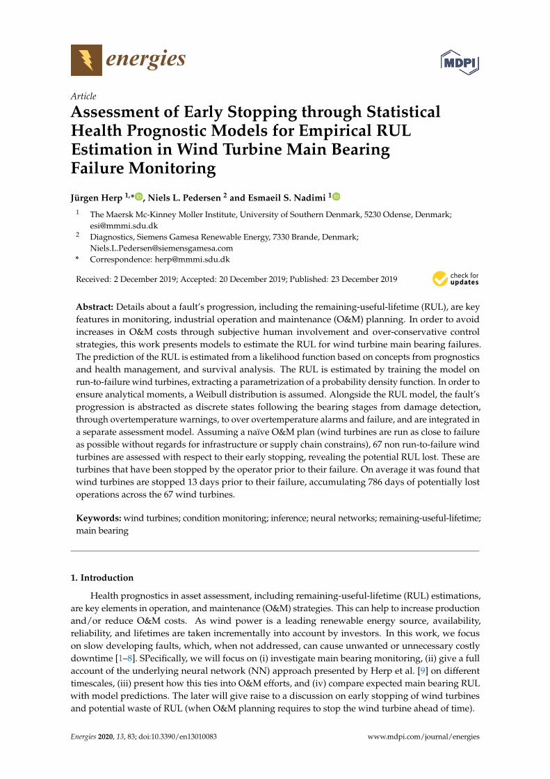
In detail, the state abstraction for the health indicator can be seen in Figure 4. From top tobottom the health indicator for a wind turbine is shown in (a), (b) shows the log-likelihood for thestate transitions (gray-scale) and its maximum likelihood, (c) shows the state transition probabilitydensity function and cumulative density function, in addition the abstracted states in accordance withEquation (21) are provided.

0.5

1.0

1.5

[a.u

.]

Health Indicator

0

100

200

s [Da

ys] arg max

0

10

20

30

log

(s(t)

x [1,

t])

0 50 100 150 200 250Time [Days]

0

2

4

6

Stat

e #/

cdf

0.0

0.5

pdf

statescdfpdf

(a)

(b)

(c)

Figure 4. State Abstraction: (a) Wind turbine health indicator. (b) log-likelihood for state transition.(c) Transition probability and states.

The state abstraction give us a measure for the length of each state. Given the time for each turbineto any state transition, the RUL probabilities can be calculated equivalent to the initial assessment forany combinations of state transitions. The implementation and results of this approach are discussedin the case study of Section 3, providing the RUL probabilities from initial detection to any of the statetransition. Figure 10).

2.2.3. Continuous Assessment: RUL Recurrent Neural Network

We employ a recurrent neural network (RNN) for the continuous assessment for maximizingthe cost function given by Equation (14) at each t. In general, this is an optimization problem offinding a function or distribution in the space of hazard function, F ∈ H, that maximizes the model’slikelihood given historical data, x[1,t]. The space of all possible closed-from distributions in H is toolarge to obtain solutions in an easy manner. Furthermore, as x[1,t] can contain any information at time t,including information of the previous states [30] the optimization for all x is computational not feasible.However, constraining the problem to a Weibull distribution and letting the Weibull distribution bedependent on x[1,t], it then follows from Equations (12) and (13), as well as Equation (14) that:

arg maxα>0,β>0

logL(α, β, RUL, ∆, x[1,t]) =t

∑i=1

(∆iα(x[1,i]) log

(RUL

β(x[1,i])

)

+ ∆i

[log(

α(x[1,i]))− log(RUL)

]−(

RULβ(x[1,i])

)α(x[1,i]) (22)

This optimization is still not feasible, as for a large dataset, each parameter needs to be obtainedthrough consideration of all historic data. In the context of Figure 5, θ can be written as a vectorθ = [α, β]>. Omitting mathematical details on node level, which can be found in a wide rangeof textbooks such as Goodfellow et al. [35], each node in Figure 5 outputs oi = g(xi, oi−1, ω0),for i = 1, . . . , t, a function of the data xt, previous output oi−1, and the networks topology ω0.The network’s output at each t will be of the form θ = m(xt, ot−1, ω) = [α, β]>, where m(·) is

Energies 2020, 13, 83 10 of 18

the mapping for the topology of the chosen RNN. Equation (22) is thus reduced to solving the gradientby back-propagation for a set of optimal or suboptimal ω:

LSTM Node

...

LSTM Node

x1

xt

θ1

θt

o0

o1

ot−1

ot

Figure 5. Schematic drawing the recurrent neural network sequence: input feature, current, previous,and future hidden states ot.

arg maxω

logL(ω, RUL, ∆, x[1,t]) =t

∑i=1

(∆i

[αi log

(RUL

βi

)+ log(αi)− log(RUL)

]−(

RULβi

)αi)

(23)

For the remainder of this study, we use a Long Short Term Memory (LSTM) RNN [35] andmaintain the topology, feature space, and optimization as in Herp et al. [9] (See Figure 6). The sequencelength is set to 7 days. An example on how predictions look like can be found in Figure 7, showingthe assumable ˆRUL and model prediction. The prediction is shown in terms of the first moment,median, and arg max of the Weibull distribution at each time t. The distribution itself is illustrated asshaded areas.

Dec Feb Apr Jun Aug Oct

Figure 6. Illustration of the RNN used to predict the RUL. Selected SCADA time-series are shownas input [9].

Energies 2020, 13, 83 11 of 18

0102030405060708090

0

20

40

60

80

0

0.01

0.02

0.03

0.04

0.05

0.06

-50

0

50

(a)

(b)

Figure 7. (a) Continuous prediction of RUL of a non run-to-failure wind turbine, compared to theexpected run-to-failure ˆRUL. (b) Mismatch between ˆRUL and the predictive distributions first moment,median, and arg max.

3. Assessment of Early Stopping—A Bearing Failure Study

This section combines the afore mentioned methodology and applies it to 67 non run-to-failurewind turbines. For each assessment, all turbines are investigated with respect to early stopping,showing the lost remaining RUL after turbine operations were stopped. The remaining turbines areused for model construction.

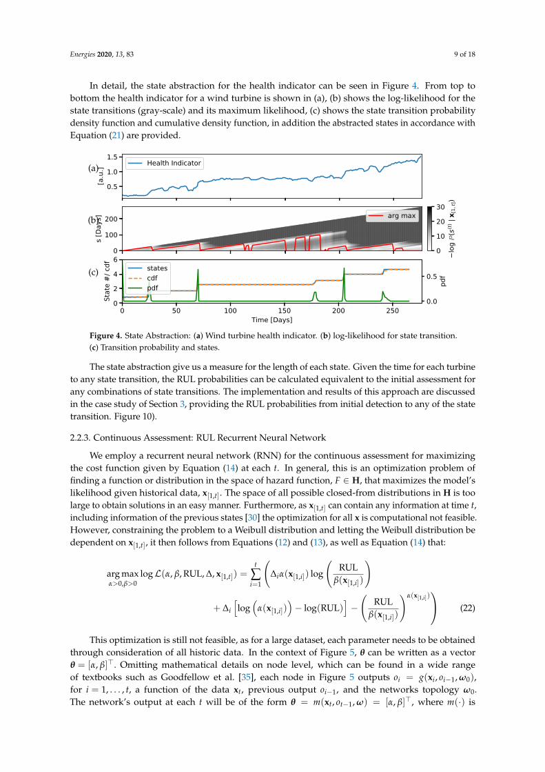
Consider the example of Figure 3 where models for the bearing overtemperature warning and bearingovertemperature alarm are illustrated. Comparing each non run-to-failure wind turbine to any of theevent models shows a mismatch δ, which is defined as the distance between any given wind turbineand the predictive models. This mismatch is interpreted as the lost remaining RUL.

Under continuous assessment, Figure 7 shows the mismatch between the presumably true ˆRULand the model prediction for a non run-to-failure wind turbine. In this case we consider an averagemeasure for each wind turbine:

D(turbine) ≡ 1T

T

∑t=1

δ(turbine)t , (24)

where

δ(turbine)t ≡ RUL(turbine)

t − ˆRUL(turbine)t . (25)

D(turbine) will then be a measure of the specific turbine’s potential remaining RUL. In the followingwe employ the methodology of this section in a case study of mean bearing failures.

When addressing whether or not to stop a wind turbine and perform maintenance is a topic on itsown. Many factors, e.g., weather condition, availability of equipment, spare parts, and manpower, haveto be taken into consideration when deciding and planing O&M tasks. In the following, we simplifytowards a pure time-based approach. Many wind turbines are stopped before they run into failure;based on the proposed RUL estimations, the potential remaining time until failure can be estimated.

Energies 2020, 13, 83 12 of 18

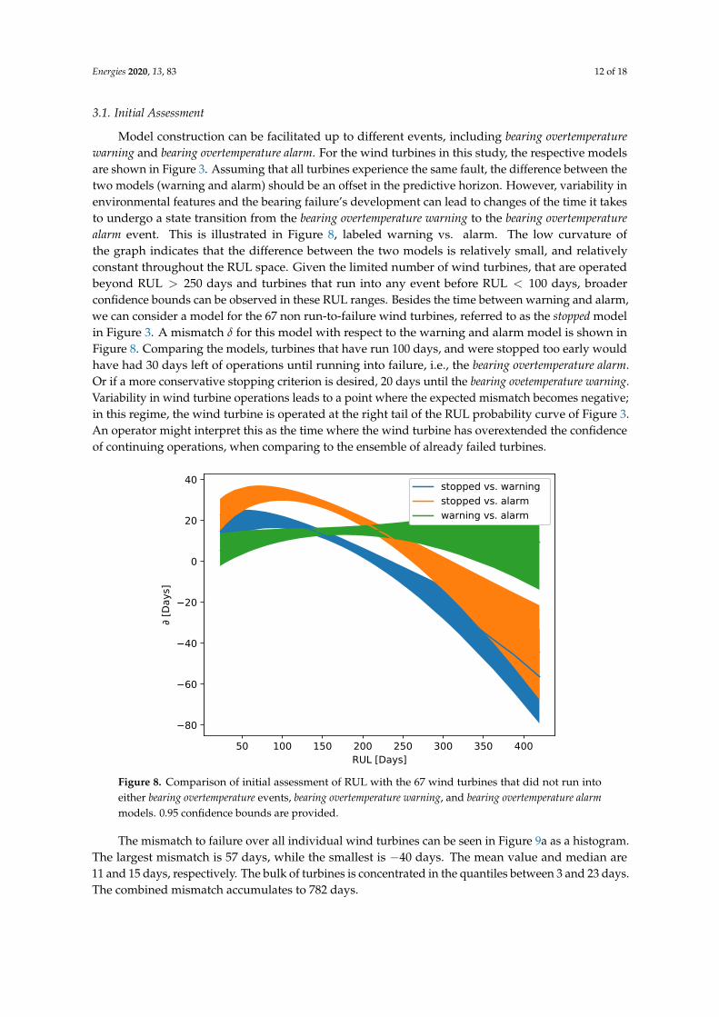
3.1. Initial Assessment

Model construction can be facilitated up to different events, including bearing overtemperaturewarning and bearing overtemperature alarm. For the wind turbines in this study, the respective modelsare shown in Figure 3. Assuming that all turbines experience the same fault, the difference between thetwo models (warning and alarm) should be an offset in the predictive horizon. However, variability inenvironmental features and the bearing failure’s development can lead to changes of the time it takesto undergo a state transition from the bearing overtemperature warning to the bearing overtemperaturealarm event. This is illustrated in Figure 8, labeled warning vs. alarm. The low curvature ofthe graph indicates that the difference between the two models is relatively small, and relativelyconstant throughout the RUL space. Given the limited number of wind turbines, that are operatedbeyond RUL > 250 days and turbines that run into any event before RUL < 100 days, broaderconfidence bounds can be observed in these RUL ranges. Besides the time between warning and alarm,we can consider a model for the 67 non run-to-failure wind turbines, referred to as the stopped modelin Figure 3. A mismatch δ for this model with respect to the warning and alarm model is shown inFigure 8. Comparing the models, turbines that have run 100 days, and were stopped too early wouldhave had 30 days left of operations until running into failure, i.e., the bearing overtemperature alarm.Or if a more conservative stopping criterion is desired, 20 days until the bearing ovetemperature warning.Variability in wind turbine operations leads to a point where the expected mismatch becomes negative;in this regime, the wind turbine is operated at the right tail of the RUL probability curve of Figure 3.An operator might interpret this as the time where the wind turbine has overextended the confidenceof continuing operations, when comparing to the ensemble of already failed turbines.

50 100 150 200 250 300 350 400RUL [Days]

80

60

40

20

0

20

40

[D

ays]

stopped vs. warning

stopped vs. alarm

warning vs. alarm

Figure 8. Comparison of initial assessment of RUL with the 67 wind turbines that did not run intoeither bearing overtemperature events, bearing overtemperature warning, and bearing overtemperature alarmmodels. 0.95 confidence bounds are provided.

The mismatch to failure over all individual wind turbines can be seen in Figure 9a as a histogram.The largest mismatch is 57 days, while the smallest is −40 days. The mean value and median are11 and 15 days, respectively. The bulk of turbines is concentrated in the quantiles between 3 and 23 days.The combined mismatch accumulates to 782 days.

Energies 2020, 13, 83 13 of 18

-60 -40 -20 0 20 40 60 800

5

10

15

δ(a) Initial Assessment

-60 -40 -20 0 20 40 60 800

5

10

15

20

25

30

35

δ(b) Discrete Assessment

-60 -40 -20 0 20 40 60 800

5

10

15

20

25

30

(c) Continuous Assessment

Figure 9. Distribution over mismatch for the 67 wind turbines that did not run into either bearingovertemperature events. (a) initial, (b) discrete, and (c) continuous assessment.

Energies 2020, 13, 83 14 of 18

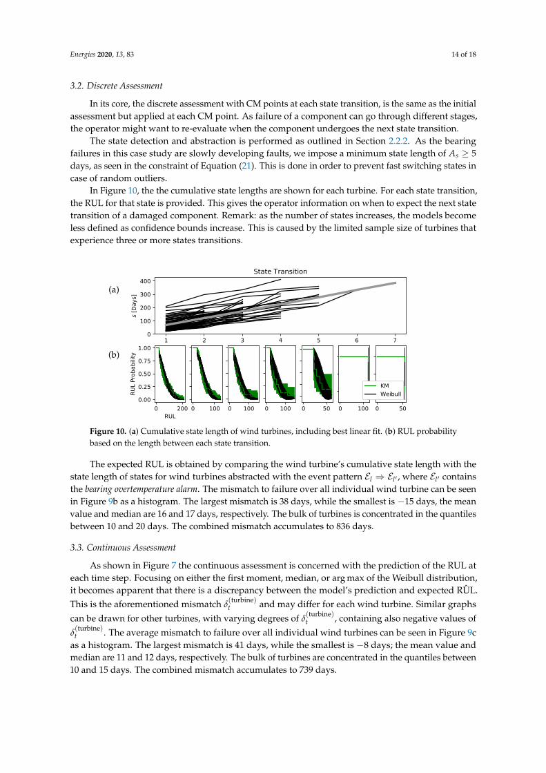
3.2. Discrete Assessment

In its core, the discrete assessment with CM points at each state transition, is the same as the initialassessment but applied at each CM point. As failure of a component can go through different stages,the operator might want to re-evaluate when the component undergoes the next state transition.

The state detection and abstraction is performed as outlined in Section 2.2.2. As the bearingfailures in this case study are slowly developing faults, we impose a minimum state length of As ≥ 5days, as seen in the constraint of Equation (21). This is done in order to prevent fast switching states incase of random outliers.

In Figure 10, the the cumulative state lengths are shown for each turbine. For each state transition,the RUL for that state is provided. This gives the operator information on when to expect the next statetransition of a damaged component. Remark: as the number of states increases, the models becomeless defined as confidence bounds increase. This is caused by the limited sample size of turbines thatexperience three or more states transitions.

1 2 3 4 5 6 70

100

200

300

400

s [D

ays]

State Transition

0 200RUL

0.00

0.25

0.50

0.75

1.00

RU

L Pro

bab

ility

0 100 0 100 0 100 0 50 0 100 0 50

KM

Weibull

(a)

(b)

Figure 10. (a) Cumulative state length of wind turbines, including best linear fit. (b) RUL probabilitybased on the length between each state transition.

The expected RUL is obtained by comparing the wind turbine’s cumulative state length with thestate length of states for wind turbines abstracted with the event pattern El ⇒ El′ , where El′ containsthe bearing overtemperature alarm. The mismatch to failure over all individual wind turbine can be seenin Figure 9b as a histogram. The largest mismatch is 38 days, while the smallest is −15 days, the meanvalue and median are 16 and 17 days, respectively. The bulk of turbines is concentrated in the quantilesbetween 10 and 20 days. The combined mismatch accumulates to 836 days.

3.3. Continuous Assessment

As shown in Figure 7 the continuous assessment is concerned with the prediction of the RUL ateach time step. Focusing on either the first moment, median, or arg max of the Weibull distribution,it becomes apparent that there is a discrepancy between the model’s prediction and expected ˆRUL.This is the aforementioned mismatch δ

(turbine)t and may differ for each wind turbine. Similar graphs

can be drawn for other turbines, with varying degrees of δ(turbine)t , containing also negative values of

δ(turbine)t . The average mismatch to failure over all individual wind turbines can be seen in Figure 9c

as a histogram. The largest mismatch is 41 days, while the smallest is −8 days; the mean value andmedian are 11 and 12 days, respectively. The bulk of turbines are concentrated in the quantiles between10 and 15 days. The combined mismatch accumulates to 739 days.

Energies 2020, 13, 83 15 of 18

4. Discussion

Common for all assessments is a high count of wind turbine mismatches at the respective meanvalues. These peaks can contain more than twice the amount of wind turbines than their neighboringbins, indicating not only the most likely mismatch, but also a firm consistency indicating a tendency tostop too early. However, two points are worth mentioning, (i) the different assessments do not yieldthe same results, and (ii) the accumulative mismatch is based on naïve O&M assumption.

4.1. Discrepancy Between Assessments

The discrepancy between the different assessments stem from the underlying nature of thedescriptive statistics. As the initial assessment applies for the total length of failure, no iterativeadjustment occurs in the monitoring effort, thus assessing wind turbines that are further into a faultprocess are not presented by the initial assessment. On the other hand, as the name implies, it gives aninitial assessment of the expected length of the failure state and their relative probability based on anensemble of wind turbines.

A step closer to a real representation of the RUL is provided by the discrete assessment. While thefailure state can be split further into shorter states, the RUL and probability of failure is obtained bypropagating non run-to-failure wind turbines through the RUL probabilities for each state transition.Besides, the discrete assessment can provide a measure of RUL until the next state transition, aiding anoperator to known when to stop a wind turbine’s operation for more conservative O&M strategies.For both the initial assessment and discrete assessment, RUL of individual wind turbines and, fromthere, the mismatch δ, are ensemble measures, i.e., when addressing the RUL of a single wind turbinewith respect to a cumulative distribution obtained by all other turbines that were undergoing thesame failure.

The initial and discrete assessments are in their core curve fitting problems for one or moredatasets of wind turbine RULs. When the number of CM points goes towards the number of samplevectors, S → T, one can consider the discrete and continuous assessment as equivalent. While theaforementioned assessment was an ensemble measure, the continuous assessment offers a real-timemonitoring approach for individual wind turbines, where the RUL is updated at each successive timestep. This makes the prediction of the RUL more and more reliable the closer a wind turbine is tofailure, but provides poor or misleading assessments early in the fault process, where predictions arewide [9]. The further a wind turbine is in a fault state, a continuous assessment becomes more andmore desirable.

All together, when combined as proposed in Figure 1, the proposed assessment offers an operatorinformation at desired stages of a main bearing fault.

4.2. The Naïve O&M Assumption

The cumulative, potential lost RUL has to be looked upon with caution. Firstly, naïve O&Massumption takes away any other consideration that might play a role in stopping a turbine,and secondly, wind turbines might continue to operate reliably even if models suggest otherwise.Apart from the predictive error due to model constraints, it becomes apparent that RUL, i.e., a measureof time, is a difficult measure that is not easily related to the physical parameters of a wind turbine’soperation. If a wind turbine is not operated due to lack of wind or other external factors, no matterhow good a model, predictions will underestimate the RUL in any of the suggested frameworks.

5. Conclusions

We have proposed three fault monitoring and assessment concepts, namely, initial assessment,discrete assessment, and continuous assessment, showing that in any of the frameworks, wind turbines arestopped earlier than necessary compared to a global ensemble. Based on the descriptive statistics of 67non-run-to-failure wind turbines, wind turbines are stopped 13 days too early, prior to their failure,

Energies 2020, 13, 83 16 of 18

accumulating, on average, 786 of potentially lost days of operations under the naïve O&M assumptionmade in this study. Future work will probably focus on the inclusion of supply chain and weatherconstraints to represent a more realistic model mismatch behavior.

Author Contributions: Conceptualization:, J.H., N.L.P. and E.S.N.; Methodology: J.H.; Resources: N.L.P.; Datacuration: J.H.; Writing—Original draft preparation: J.H.; Writing—review and editing, J.H.; Supervision, E.S.N.All authors have read and agreed to the published version of the manuscript.

Funding: This project was funded by Siemens Gamesa Renewable Energy and the University of Southern Denmark.

Acknowledgments: The authors would like to take the chance to thank Siemens Gamesa Renewable Energy forproviding us with the necessary data.

Conflicts of Interest: The authors declare no conflict of interest. The funders had no role in the design of thestudy; in the collection, analyses, or interpretation of data; in the writing of the manuscript, or in the decision topublish the results.

Abbreviations

cdf cumulative distribution functionCM Condition MonitoringKM Kaplan-MeierNN Neural NetworkO&M Operation and Maintenancepdf probability density functionRNN Recurrent Neural NetworkRUL Remaining-Useful-LifetimeSCADA Supervisory Control and Data Acquisition

Nomenclature

a scalara vectorA matrixxt sample vectorx[a,b] samples on the interval a to bE set of all possible eventsEk kth eventEl subset of ERUL random variable for the remaining-useful-lifetime

ˆRUL real remaining-useful-lifetimeη hazard functionH cumulative hazard function∆ ∈ {0, 1} censoring variableL likelihood functionβ = [βc, βm] hyper-parameter for conditional prior and sample modelP(s(t) | s(t−1)) ≡ P(s(t) | s(t−1), βc) independent conditional priorP(s(t) | x[1,t]) probability distribution over the current stateP(xt | s(t−1), x[1,t−1]) ≡ P(xt | s(t−1), x[1,t−1], βm) sample modelδ mismatch between RUL and ˆRULD average mismatch

References

1. Petersen, K.R.; Madsen, E.S.; Bilberg, A. Offshore Wind Power at Rough Sea: The need for new MaintenanceModels. In Proceedings of the 20th EurOMA Conference, Dublin, Ireland, 9–12 June 2013.

2. Nielsen, J.; Sørensen, J. On risk-based operation and maintenance of offshore wind turbine components.Reliab. Eng. Syst. Saf. 2011, 96, 218–229, doi:10.1016/j.ress.2010.07.007. [CrossRef]

Energies 2020, 13, 83 17 of 18

3. Blanco, M.I. The economics of wind energy. Renew. Sustain. Energy Rev. 2009, 13, 1372–1382,doi:10.1016/j.rser.2008.09.004. [CrossRef]

4. van Bussel, G.J.W.; Zaaijer, M.B. Reliability, Availability and Maintenance Aspects of Large-Scale OffshoreWind Farms, a Concepts Study. In Proceedings of the MAREC 2001 Marine Renewable Energies Conference,Newcastle, UK, 27 March 2001; Volume 113, pp. 119–126.

5. Wilkinson, M.; Spinato, F.; Knowles, M. Towards the Zero Maintenance Wind Turbine. In Proceedings of the41st International Universities Power Engineering Conference (UPEC ’06), Newcastle, UK, 6–8 Septemeber 2006;Volume 1, pp. 74–78, doi:10.1109/UPEC.2006.367718. [CrossRef]

6. Kim, N.; An, D.; Choi, J. Prognostics and Health Management of Engineering Systems: An Introduction; Springer:Berlin, Germany, 2016.

7. Sheppard, J.W.; Kaufman, M.A.; Wilmer, T.J. IEEE Standards for Prognostics and Health Management.IEEE Aerosp. Electron. Syst. Mag. 2009, 24, 34–41, doi:10.1109/MAES.2009.5282287. [CrossRef]

8. Walford, C.A. Wind Turbine Reliability: Understanding and Minimizing Wind Turbine Operation and MaintenanceCosts; Technical Report SAND2006-1100; Sandia National Laboratories: Albuquerque, NM, USA, 2006.Available Online: https://energy.sandia.gov/wp-content/gallery/uploads/SAND-2006-1100.pdf (accessedon 12 December 2019).

9. Herp, J.; Pedersen, N.L.; Nadimi, E.S. A Novel Probabilistic Long-Term Fault Prediction FrameworkBeyond SCADA Data—With Applications in Main Bearing Failure. J. Phys. Conf. Ser. 2019, 1222, 012043,doi:10.1088/1742-6596/1222/1/012043. [CrossRef]

10. Trappey, A.J.C.; Trappey, C.V.; Ma, L.; Chang, J.C. Integrating Real-Time Monitoring and Asset HealthPrediction for Power Transformer Intelligent Maintenance and Decision Support. In Engineering AssetManagement—Systems, Professional Practices and Certification; Tse, P.W., Mathew, J., Wong, K., Lam, R., Ko, C.,Eds.; Springer: Cham, Switzerland, 2015; pp. 533–543.

11. You, G.W.; Park, S.; Oh, D. Diagnosis of Electric Vehicle Batteries Using Recurrent Neural Networks.IEEE Trans. Ind. Electron. 2017, 64, 4885–4893, doi:10.1109/TIE.2017.2674593. [CrossRef]

12. Herp, J.; Ramezani, M.H.; Bach-Andersen, M.; Pedersen, N.L.; Nadimi, E.S. Bayesian state prediction ofwind turbine bearing failure. Renew. Energy 2018, 116, 164–172, doi:10.1016/j.renene.2017.02.069. [CrossRef]

13. Hong, S.; Zhou, Z.; Zio, E.; Wang, W. An adaptive method for health trend prediction of rotating bearings.Dig. Signal Process. 2014, 35, 117–123, doi:10.1016/j.dsp.2014.08.006. [CrossRef]

14. Si, X.S. An Adaptive Prognostic Approach via Nonlinear Degradation Modeling: Application to BatteryData. IEEE Trans. Ind. Electron. 2015, 62, 5082–5096, doi:10.1109/TIE.2015.2393840. [CrossRef]

15. Khan, S.; Yairi, T. A review on the application of deep learning in system health management. Mech. Syst.Signal Process. 2018, 107, 241–265, doi:10.1016/j.ymssp.2017.11.024. [CrossRef]

16. Katzman, J.; Shaham, U.; Bates, J.; Cloninger, A.; Jiang, T.; Kluger, Y. DeepSurv: Personalized TreatmentRecommender System Using A Cox Proportional Hazards Deep Neural Network. BMC Med. Res. Methodol.2018, 18, 24. [CrossRef]

17. Si, X.; Zhang, Z.; Hu, C. Data-Driven Remaining Useful Life Prognosis Techniques: Stochastic Models, Methods andApplications; Springer Series in Reliability Engineering; Springer: Berlin/Heidelberg, Germany, 2017.

18. Márquez, F.P.G.; Tobias, A.M.; Pérez, J.M.P.; Papaelias, M. Condition monitoring of wind turbines: Techniquesand methods. Renew. Energy 2012, 46, 169–178, doi:10.1016/j.renene.2012.03.003. [CrossRef]

19. Ranganath, R.; Tang, L.; Charlin, L.; Blei, D.M. Deep Exponential Families. arXiv 2014, arxiv:1411.2581.20. Ranganath, R.; Perotte, A.; Elhadad, N.; Blei, D. Deep Survival Analysis. arXiv 2016, arXiv:1608.02158.21. Ali, J.B.; Chebel-Morello, B.; Saidi, L.; Malinowski, S.; Fnaiech, F. Accurate bearing remaining useful life

prediction based on Weibull distribution and artificial neural network. Mech. Syst. Signal Process. 2015,56–57, 150–172, doi:10.1016/j.ymssp.2014.10.014. [CrossRef]

22. Mazhar, M.; Kara, S.; Kaebernick, H. Remaining life estimation of used components in consumer products:Life cycle data analysis by Weibull and artificial neural networks. J. Op. Manag. 2007, 25, 1184–1193,doi:10.1016/j.jom.2007.01.021. [CrossRef]

23. Yang, Z.; Chen, C.; Wang, J.; Li, G. Reliability Assessment of CNC Machining Center Based on WeibullNeural Network. Math. Probl. Eng. 2015, 2015, 8. [CrossRef]

24. Aggarwal, K.; Atan, O.; Farahat, A.K.; Zhang, C.; Ristovski, K.; Gupta, C. Two Birds with One Network:Unifying Failure Event Prediction and Time-to-failure Modeling. In Proceedings of the 2018 IEEEInternational Conference on Big Data (Big Data), Seattle, WA, USA, 10–13 December 2018; pp. 1308–1317.

Energies 2020, 13, 83 18 of 18

25. Bach-Andersen, M.; Rømer-Odgaard, B.; Winther, O. Flexible non-linear predictive models for large-scalewind turbine diagnostics. Wind Energy 2016, 20, 753–764, doi:10.1002/we.2057. [CrossRef]

26. Kleinbaum, D.; Klein, M. Survival Analysis: A Self-Learning Text, 3rd ed.; Statistics for Biology and Health;Springer: New York, NY, USA, 2011.

27. Patti, S.; Biganzoli, E.; Boracchi, P. Review of the Maximum Likelihood Functions for Right Censored Data.A New Elementary Derivation. In COBRA Preprint Series; bepress: Berkeley, CA, USA, 2007.

28. Kaplan, E.L.; Meier, P. Nonparametric Estimation from Incomplete Observations. J. Am. Stat. Assoc. 1958,53, 457–481, doi:10.1080/01621459.1958.10501452. [CrossRef]

29. Herp, J.; Ramezani, M.H. State transition of wind turbines based on empirical inference on model residuals.In Proceedings of the 2015 Conference on Research in Adaptive and Convergent Systems, RACS 2015,Prague, Czech Republic, 9–12 October 2015; pp. 32–37, doi:10.1145/2811411.2811509. [CrossRef]

30. Herp, J.; Ramezani, M.H.; Nadimi, E. Dependency in State Transitions of Wind Turbines-Inference on modelResiduals for State Abstractions. IEEE Trans. Ind. Electron. 2017, doi:10.1109/TIE.2017.2674580. [CrossRef]

31. Prescott Adams, R.; MacKay, D.J.C. Bayesian Online Changepoint Detection. arXiv 2007, arXiv:0710.3742.32. Fisher, R.A. On the Mathematical Foundations of Theoretical Statistics. Philos. Trans. R. Soc. Lond. A Math.

Phys. Eng. Sci. 1922, 222, 309–368, doi:10.1098/rsta.1922.0009. [CrossRef]33. Hipp, C. Sufficient Statistics and Exponential Families. Ann. Stat. 1974, 2, 1283–1292, doi:10.1214/aos/1176342879.

[CrossRef]34. Fisher, R.A. Applications of “Student’s” distribution. Metron 1925, 5, 90–104.35. Goodfellow, I.; Bengio, Y.; Courville, A. Deep Learning; MIT Press: Cambridge, MA, USA, 2006. Available

online: http://www.deeplearningbook.org (accessed on 12 December 2019)

c© 2019 by the authors. Licensee MDPI, Basel, Switzerland. This article is an open accessarticle distributed under the terms and conditions of the Creative Commons Attribution(CC BY) license (http://creativecommons.org/licenses/by/4.0/).