assessment of csp+d potential in the mena area · market shares of the three main desalination...
TRANSCRIPT
SolarPACES Task VI Activity:
Solar Energy & Water Processes
and Applications
ASSESSMENT OF CSP+D POTENTIAL IN THE
MENA AREA
Activity duration:
Period covered by the report:
Date of preparation:
Project participants:
Authors:
Revision:
Number of pages (inc. cover):
01.04.2010 – 30.09.2012
01.04.2010 – 30.09.2012
02.04.2013
CIEMAT, DLR, NREA
J. Blanco, D. Alarcón, P. Palenzuela (CIEMAT)
C. Sattler, M. Moser, R. Olwig (DLR)
L. Georgi, R. El Navrawy, B. Rashed (NREA)
1
67
2
Content
List of Figures ........................................................................................................................... 3
1. Review of conventional power and water cogeneration plants .......................................... 9
1.1. The Desalination market and technology shares ......................................................... 9
1.2. Desalination technology .............................................................................................. 9
1.2.1. Multi stage flash Distillation (MSF) .................................................................... 9
1.2.2. Multiple Effect Distillation (MED) with or without Thermal Vapour
Compression (TVC) .......................................................................................................... 11
1.2.3. Reverse Osmosis (RO) ....................................................................................... 12
1.3. Cogeneration of Power and Water ............................................................................. 13
1.3.1. Conventional -Fossil Fuel based- Cogeneration Plants ...................................... 13
1.3.2. Cogeneration with Concentrating Solar Power Plants ....................................... 14
2. Solar resource assessment in the Egypt coastal strip ........................................................ 16
2.1. Introduction and context ............................................................................................ 16
2.2. Definition of geographical locations for the solar resource assessment .................... 17
2.3. Methodology for solar radiation derived from satellite images ................................ 18
2.4. Results and comments ............................................................................................... 20
3. Feasible configuration options to CSP+D cogeneration plants ........................................ 22
3.1. Introduction ............................................................................................................... 22
3.2. Description of the systems ......................................................................................... 22
3.3. Analysis of the systems ............................................................................................. 26
3.4. Economic analysis ..................................................................................................... 29
3.5. Results ....................................................................................................................... 30
3.5.1. Thermodynamic analysis .................................................................................... 30
3.5.2. Economic analysis .............................................................................................. 33
4. Feasibility study of CSP+D integrated plant in Port Safaga............................................. 35
4.1. Site location selection ................................................................................................ 35
4.2. Analysis of the systems ............................................................................................. 37
4.2.1. Calculation of steam condensation temperature ................................................. 38
4.2.2. Calculation of the internal water consumption .................................................. 45
4.3. Economic analysis ..................................................................................................... 47
4.4. Results ....................................................................................................................... 50
4.4.1. Thermodynamic analysis .................................................................................... 50
4.4.2. Economic analysis .............................................................................................. 51
4.5. Additional Report – Yearly Simulation Draft ........................................................... 54
4.5.1. Steady-State Operating Performance ................................................................. 55
4.5.2. Annual Simulation and Economical Calculation ............................................... 57
5. Conclusions: potential of CSP+D concept at Egypt and MENA countries ...................... 62
6. References ......................................................................................................................... 64

3
List of Figures
Figure 1-1. Market shares of the three main desalination technologies MSF, MED and RO
in 2010. Total global desalination capacity at this year was 66.4 Mio m³/d, Source:
GWI and DesaData/IDA ............................................................................................... 9
Figure 1-2. Flowsheet of a MSF Desalination system, Source: Dr. Heike Glade, University of
Bremen ........................................................................................................................ 10
Figure 1-3. The principle of Multi-Effect-Distillation (MED), Source: Dr. Heike Glade,
University of Bremen .................................................................................................. 11
Figure 1-4. The principle of Multi-Effect-Distillation (MED) with Thermal vapour
compression (TVC), Source: Dr. Heike Glade, University of Bremen ....................... 12
Figure 1-5. Cogeneration configuration with steam turbines (backpressure (BP) or
controlled extraction condensing turbines (EC) (SIDEM website) ............................ 13
Figure 1-6. Cogeneration configuration with a gas turbine and a heat recovery steam
generator (SIDEM website) ........................................................................................ 14
Figure 1-7. Combined cycle cogeneration configuration comprising a gas turbine with heat
recovery steam generator and a steam turbine (BP or EC) (SIDEM website) .......... 14
Figure 1-8. Sketch of a condensation turbine (Toshiba website) ........................................... 15
Figure 1-9. Sketch of a back-pressure turbine (Toshiba website) ......................................... 15
Figure 2-1. Egypt coastal strip at the Mediterranean Sea in red colour (drawn by Google
Earth) .......................................................................................................................... 17
Figure 2-2. Elevation profile of the Egypt coastal strip at the Mediterranean Sea ............... 17
Figure 2-3. Egypt coastal strip at the Red Sea, the red line inland corresponds to the Egypt
border drawn by Google Earth .................................................................................. 18
Figure 2-4. Elevation profile of the Egypt coastal strip at the Red Sea ................................. 18
Figure 2-5. DNI results of the Egypt coastal strip at the Mediterranean sea ....................... 20
Figure 2-6. DNI results of the Egypt coastal strip in the west side of the Red sea ................ 21
Figure 3-1. Diagram of the LT-MED unit integration into a PT-CSP plant .......................... 23
Figure 3-2. Diagram of the LT-MED-TVC unit integration into a PT-CSP plant. (a) The
steam is extracted from the HP turbine (b) The steam is extracted from LP turbine . 24
Figure 3-3. Diagram of the RO unit integration into a PT-CSP plant ................................... 24
Figure 3-4. Simplified calculation scheme ............................................................................. 27
Figure 3-5. Direct normal radiation at design day in Port Safaga (Egypt) ........................... 28
Figure 3-6. Comparison of the thermal power obtained in configuration 2 (for every steam
extracted pressure) to the one obtained in configuration 3........................................ 32
Figure 3-7. Comparison of the overall efficiency obtained in configuration 2 (for every steam
extracted pressure) to the one obtained in configuration 3........................................ 32
Figure 3-8. Comparison of the thermal power dissipated in the condenser in conf. 2 (for
every steam extracted pressure) to the one obtained in configuration 3 .................... 32

4
Figure 3-9. Comparison between the solar field in configuration 2 (for every steam extracted
pressure) to the one obtained in configuration 3 ....................................................... 32
Figure 3-10. Motive steam and entrained vapour mass flow rates for every pressure of the
steam extracted from the LP turbine in configuration 2 ............................................ 33
Figure 4-1. Port Safaga geographical coordinates: 26º45’ North, 33º56’ East [Google
Earth, 2013] ............................................................................................................... 35
Figure 4-2. Initial selected locations of the CSP+D cogeneration plant in Port Safaga ....... 36
Figure 4-3. View of final selected location, about 10 km north of Port Safaga ..................... 36
Figure 4-4. Scheme of a Once-Through cooling system [Tawney, 2003] .............................. 39
Figure 4-5. Scheme of a dry (air) cooling system [Tawney, 2003] ........................................ 40
Figure 4-6. Bottom of an evaporative tower (wetcooling.com) .............................................. 41
Figure 4-7. Scheme of an Evaporative Tower cooling system [Tawney, 2003] ..................... 41
Figure 4-8. Distribution of wet and dry bulb temperature as function of relative humidity
[Data from Meteonorm] ............................................................................................. 43
Figure 4-9. Frequency of dry bulb and wet bulb temperatures in Port Safaga [Data from
Meteonorm] ................................................................................................................ 43
Figure 4-10. Percentage of water consumed in a solar thermal power plant with evaporative
cooling ........................................................................................................................ 46
Figure 4-11. Variation of the LEC with the cost of the solar field ......................................... 54
Figure 4-12. Land use estimation and solar field size ............................................................ 55
Figure 4-13. Design power and water production under the assumption of identical water
production for RO and MED (turbine inlet heat: 180 MWth) ..................................... 56
Figure 4-14. Design power and water production under the assumption of identical water
production for RO and MD (turbine inlet heat: 180 MWth) ....................................... 57
Figure 4-15. Overview of calculation scheme for annual yield analysis with hourly time step
.................................................................................................................................... 58
Figure 4-16. Energy flow diagram for the CSP-OTC+RO (left) and CSP+MED (right)
configurations ............................................................................................................. 59
Figure 4-17. LEC and LWC for the analysed configurations ................................................. 60
Figure 4-18. LEC sensitivity on CO2 costs ............................................................................. 60
Figure 4-19. LEC sensitivity on storage capacity (configuration CSP-OTC + RO) .............. 61

5
List of Tables
Table 1-1. Technical characteristics of different desalination technologies ......................... 13
Table 3-1. Operating conditions and assumptions used in the thermodynamic simulation of
analyzed configurations 1, 2 and 3 ............................................................................. 25
Table 3-2. LS-3 collector characteristics ............................................................................... 28
Table 3-3. Assumptions made to calculate the cost of the CSP plant & RO facility .............. 30
Table 3-4. Net Output Thermal Capacity (NOTC), overall efficiency, cooling requirements,
number of collector per row, number of rows, aperture area resulting from each
diagram proposed ....................................................................................................... 31
Table 3-5. Comparative costs of power (50 MWe net production) and water (35018 m3/day
net production) cogeneration with PT-CSP/RO and PT-CSP/LT-MED configurations
.................................................................................................................................... 33
Table 4-1. Overview of analyzed configurations .................................................................... 35
Table 4-2. Summary of most relevant solar field geometry and design assumptions [Hirsch,
2010] ........................................................................................................................... 37
Table 4-3. Monthly values of seawater and air temperature and relative humidity
[holydaycheck.com, NREA] ........................................................................................ 39
Table 4-4. Overview on relevant data for different cooling techniques ................................. 40
Table 4-5. Specific internal electricity consumption of the analyzed cooling systems .......... 45
Table 4-6. Water consumption ............................................................................................... 46
Table 4-7. Summary of the cost assumptions ......................................................................... 47
Table 4-8. Input data to calculate the direct capital costs ..................................................... 47
Table 4-9. Input data to calculate the indirect project costs .................................................. 48
Table 4-10. Input data to calculate the costs manpower ....................................................... 48
Table 4-11. Input data to calculate the operation and maintenance costs ............................ 48
Table 4-12. Input data to calculate the operation costs gas consumption ............................. 49
Table 4-13. Input data to calculate other yearly fixed costs .................................................. 49
Table 4-14. Summary table with main power cycle parameters ............................................ 50
Table 4-15. Summary table with water consumptions ........................................................... 51
Table 4-16. Annual analysis of the CSP plant ........................................................................ 52
Table 4-17. Annual analysis of the desalination plant ........................................................... 52
Table 4-18. Investment Cost results for the CSP and DES plants ......................................... 52
Table 4-19. Annual costs of the CSP plant ............................................................................. 53
Table 4-20. Annual costs of the desalination plant ................................................................ 53
Table 4-21. Results of the power and water costs .................................................................. 53
Table 4-22. Main results from annual yield simulation for the analysed configurations ...... 59

6
List of Abbreviations
ACC Air Cooled Condenser
AOD Aerosol Optical Depth
BP Backpressure turbine
BSRN Baseline Surface Radiation Network
CSP+D Concentrating Solar Power and Desalination
DNI Direct Normal Irradiance
EC Controlled Extraction Condensing turbine
EES Engineering Equation Solver
Enet Annual net electricity delivered to the grid
FLH Annual Full Load operating Hours
FWH Feed Water Heater
GHI Global Horizontal Irradiance
GOR Gain Output Ratio
HRV High Resolution Visible channel
HP High pressure
HTF Heat Transfer Fluid
IAM Incident Angle Modifier
IEA International Energy Agency
LEC Levelized Electricity Cost
LT-MED Low temperature multi-effect distillation
LT-MED-TVC Low temperature multi-effect distillation powered by a thermal vapour
compressor
LP Low pressure
LWC Levelized Water Cost
MD Membrane Distillation
MED Multi Effect Distillation
MENA Middle East and North Africa
MSF Multi Stage Flash Distillation
NOTC Net output thermal capacity
OTC Once-Through Cooling
PB Power Block
PRH Power required by the reheaters of the cycle
PT Parabolic Trough
RO Reverse Osmosis
RMSE Root Mean Square Error
SF Solar Field
ST Steam Turbine
TES Thermal Energy Storage
TVC-MED Thermal Vapor Compression Multi-Effect Distillation

7
List of Symbols
cpcw Specific heat of cooling water
Steam latent heat of condensation
Enet Annual net electricity delivered to the grid
kd Real debt interest rate
Kfuel Annual fuel cost
Kinsurance Annual insurance rate
Kinvest Total investment of the plant
KO&M Annual operation and maintenance costs
mw Feed water mass flow
mcw Cooling water mass flow
ms_turb_out Steam mass flow at the turbine outlet
n Depreciation period in years ηturb_th Thermal efficiency of the power cycle ηturb_gross Gross efficiency of the power cycle ηturb_net (CSP w/o TES) Net efficiency of the power cycle ηturb_sys (inc DES.) Global efficiency of the system
pump Heat Transfer Fluid pump efficiency
Pdesal Power required by the desalination plant (MW) Pgross Gross power production of the CSP+D system
Pnet Net power production of the CSP+D system (MW)
Ppcs Power required by the power conversion system (MW)
Ppumps Power required by the pumps (MW)
Pparasitics_turb Internal power consumption of the steam turbine
Pparasitics_sf Power consumption for HTF pumping (solar field) Ppar_SF Power consumption for HTF pumping (solar field) Ppar_TES Power consumption of the Thermal Energy Storage Ppar_TURB Power consumption for water pumping (power block) Ppar_COOL Power consumption for cooling (power block)
HTF Heat Transfer Fluid density
Qturb_out Heat flow at the turbine outlet
Qturb_in Heat flow at the turbine inlet
xs_out Steam moisture fraction at the turbine outlet

8
FIRST PHASE
Assessment of possible configurations of CSP+D
to optimize the production of water and electricity
within the MENA region

First Phase: Assessment of CSP+D potential in the MENA area SolarPACES Task VI Activity
9
1. Review of conventional power and water cogeneration plants
1.1. The Desalination market and technology shares
The worldwide desalination market is basically dominated by three desalination technologies:
reverse osmosis (RO), multi-stage flash distillation (MSF) and multiple-effect distillation
(MED). According to GWI, at the end of 2010 total installed desalination capacity in
operation worldwide reached 66.4 Mio m³/d, having RO, prevalent seawater desalination
process, around 60% of this capacity. Thermal MSF and MED desalination technologies are
based on water evaporation, with a respective quota of 26% and 8.2%, see Figure 1-1. This
difference is due to the biggest capacity production of MSF technology, besides the higher
thermodynamic efficiency of MED. Single-unit capacities of MSF plants range from 5000 to
76,000 m³ per day. The rest of desalination technologies, starting by Electrodialysis (ED) has
much lower installed capacities. ED is not applicable to seawater.
Figure 1-1. Market shares of the three main desalination technologies MSF, MED and RO in 2010. Total
global desalination capacity at this year was 66.4 Mio m³/d, Source: GWI and DesaData/IDA
The worldwide installed capacity of MED, MED-TVC and MVC processes was 5.4 Mio. m³
fresh water per day in 2010. Single-unit capacities of MED plants without vapour
compression range from 100 m³ to 15,000 m³ of distillate per day. Bigger plants with a single-
unit capacity of up to 36,000 m³ per day are mostly built with thermal vapour compression.
All MED plants (including TVC and MVC) operate at low temperatures of less than 70°C to
limit corrosion and scaling. The thermal energy consumption of MED plants ranges from 185
to 65 kWh per ton of distillate, for MED-TVC plants from 80 to 45 kWh per ton of distillate.
The required heating steam pressure for MED plants is less than 0.35 bars. Alternatively the
use of hot water is possible. The required motive steam pressure for the steam ejector in
MED-TVC plants ranges from 2 to 20 bars. MED and MED-TVC plants have an electrical
energy consumption between 1 and 2 kWh per ton of distillate.
1.2. Desalination technology
1.2.1. Multi stage flash Distillation (MSF)
Figure 1-2 shows a MSF plant. As the name implies, MSF plants consist of several (around 16
to 22) flash chambers. Seawater is heated to the so called top brine temperature in the
condensers of the single stages by condensing vapour on the outside of the condenser tubes

First Phase: Assessment of CSP+D potential in the MENA area SolarPACES Task VI Activity
10
and, finally, in the brine heater, using steam from an external source. The hot seawater is fed
to the first flash chamber, where the pressure is maintained slightly below the saturation
pressure of the water. A fraction of the water flashes, the generated vapour passes through a
mist eliminator, condenses on the outside surface of the condenser tubes and the condensate is
collected in the distillate trough. Inside the condenser tubes the seawater is preheated. The
same principles recur in the next stages with a subsequently lower pressure in each stage.
There are mainly two MSF process configurations. In recycle distillers, which are exclusively
employed today, the seawater is preheated in the condensers of the last 2 to 4 stages of the
plant, called heat rejection section. Then part of the seawater, the cooling water, is discharged
to the sea and the remaining seawater, the make-up water, is deaerated. After deaeration the
make-up water is mixed with part of the brine from the last stage and the so called
recirculation flow is further preheated in the condensers of the heat recovery section and in
the brine heater. The remaining brine from the last stage, which is not recycled, is discharged
back to the sea.
Figure 1-2. Flowsheet of a MSF Desalination system, Source: Dr. Heike Glade, University of Bremen
In practice, only a small percentage of the seawater is converted to steam, depending on the
ambient pressure maintained in the vessel, since vaporisation swiftly causes the water to cool
to below boiling point. Thus, multi-stage distillation makes use of a series of stages set at
increasingly lower atmospheric pressures, allowing the feed water to pass from one to
another, repeatedly flashing, without adding more heat. However, there are limits on the
number of stages, since one of the major factors affecting the thermal efficiency of MSF
plants is the temperature difference between the brine heater and the final condenser at the
cold end of the plant. While operating a plant at the upper temperature limit of 120°C leads to
increased efficiency, it also increases the potential for detrimental scale formation and
accelerated corrosion of metal surfaces
At present MSF plants operate at less than 120°C to limit scale formation. The top brine
temperature is typically between 100°C and 112°C. To obtain this temperature, a heating
steam pressure of less than 2.5 bars is required. The thermal energy consumption of MSF
plants ranges from 90 to 70 kWh per ton of distillate. MSF plants have an electrical energy
consumption of 3.5-5 kWh per ton of distillate mainly for pumping the large liquid streams.
recycledbrine
distillateblow-down
recirculation flow
make-up flow
heat recovery section
brine heater
condensate
heating steam
to the vacuum system
seawater
heat rejectionsection
deaerator
coolingwater

First Phase: Assessment of CSP+D potential in the MENA area SolarPACES Task VI Activity
11
1.2.2. Multiple Effect Distillation (MED) with or without Thermal Vapour
Compression (TVC)
Multiple-effect distillation (MED) is widely and increasingly employed for seawater
desalination. In contrast to MSF plants, the major part of the water in MED plants is not
flashed, but evaporated on heat transfer tubing. Heating steam from an external source is only
needed in the first stage, also called effect. The vapour, which is produced in the first effect, is
fed into the tubes of the next effect. It condenses inside the tubes, while a fraction of the
seawater on the outside of the tubes evaporates. The pressure is subsequently reduced from
effect to effect. Figure 1-3 shows a MED plant with four effects.
MED plants typically consist of 4 to 12 effects (3 to 8 for MED-TVC). Today mainly
horizontal tube falling film evaporators are used, in which the preheated seawater is sprayed
on a tube bundle. The water forms a thin layer on the surface of the tubes. It is heated to the
evaporating temperature on the first tubes. A fraction of the water evaporates on the rest of the
tubes. The vapour mixes with a small amount of additional vapour, originating from the
flashing brine in the bottom of the effect. After passing through a mist eliminator the vapour
is fed into the tubes of the next effect. Inside the tubes the vapour from the previous effect
condenses, while a fraction of water evaporates on the outside of the tubes.
The process of evaporation-plus-condensation is repeated from effect to effect with a
subsequently lower pressure in each effect. An ejector system extracts non-condensable gases
to maintain the vacuum in the effects.
Figure 1-3. The principle of Multi-Effect-Distillation (MED), Source: Dr. Heike Glade, University of Bremen
Evaporation plants are often built with thermal or mechanical vapour compression. In MED
plants with thermal vapour compression (MED-TVC) part of the vapour from the last or an
intermediate effect is compressed in a steam ejector and used as heating steam in the first
effect.
Figure 1-4 shows the system configuration of a MED-TVC plant. A steam ejector is added to
the MED plant to compress part of the steam produced in the last or in one of the central
effects by means of motive steam. The suction steam together with the motive steam is used
as heating steam in the first effect. Thermal vapour compression increases the thermal
efficiency of a MED plant. The steam ejector requires motive steam of at least 2 bars from an
external source.
heating steam
condensate
blow-down sea-water
distillate
finalcondenser
cooling waterfeed water

First Phase: Assessment of CSP+D potential in the MENA area SolarPACES Task VI Activity
12
Figure 1-4. The principle of Multi-Effect-Distillation (MED) with Thermal vapour compression (TVC), Source:
Dr. Heike Glade, University of Bremen
1.2.3. Reverse Osmosis (RO)
RO is by far the most widespread type of membrane-based desalination process. It is even
increasing desalination market share due to the high energy efficiency of modern plants
implementing energy recovery devices and to the possibility of scaling up plant size to
capacities in the range of 100,000 m3 per day. Commercially available RO membranes can
retain about 98-99.5% of the salt dissolved in the feed water. They are typically operated in
the pressure range between 10 and 15 bars for brackish water and around 70 bars for seawater
[Fritzmann et al. 2007].
RO is a pressure-driven process that relies on the properties of semi-permeable membranes to
separate water from a saline feed. The end result of reverse osmosis comprises the separated
flows of freshwater permeate and concentrated brine. Smooth operation and stable long-term
performance of RO membranes for seawater desalination require high quality feed water. In
presence of a poorly pre-treated feed, inorganic and organic matter may accumulate at the
membrane surface causing membrane scaling and fouling, and strongly reducing or inhibiting
mass transfer through the membranes. Conventional RO pre-treatment consists of both
physical and chemical processes. Physical pre-treatment generally consists of mechanical
filtering of the feed water by screening, cartridge filters and sand filters [Fritzmann et al.
2007]. For chemical pre-treatment scale inhibitors, coagulants, disinfectants, and
polyelectrolytes are added [Fritzmann et al. 2007].
The first step in desalinating seawater is pre-treatment. This is intended to reduce salt
precipitation or microorganism growth in membranes. RO involves forcing seawater through
a fine-pored membrane using a pressure pump at varying pressures of 67 bar to 75 bar. The
RO membranes consist of dense barrier layers of polymer matrix, through which most of the
separation occurs. Water molecules pass through these pores, while salt and impurities are
retained. Table 1-1 summarizes the technical performance characteristics of the three main
large scale and commercial desalination technologies.
heating steam
condensate
blow-down distillate
finalcondenser
cooling water
steamejector motive steam
sea-water
feed water
First Phase: Assessment of CSP+D potential in the MENA area SolarPACES Task VI Activity
13
Table 1-1. Technical characteristics of different desalination technologies
Concept Units MSF MED RO
Single unit capacity m3/d 5000 − 76000 100 − 36000 1 − 10000
Number of stages - … 16 – 22 … 4 – 12
TVC: mostly 3 − 6 -
Top brine temperature ºC < 120 < 70 < 40
Concentration factor - 1.3 − 1.5 1.3 − 1.5 1.5 − 2
Performance ratio kg/2326 kJ 7 − 9 3.5 – 10
with TVC: 8 − 14 -
Thermal energy consumption kWht/m3 90 – 70
3.5 – 10
with TVC: 80 − 45 -
Electrical energy consumption kWhe/m3 3.5 − 5 1 − 2 3,0 − 8
Specific investment costs €/(m3/d) 1000 − 1600 900 − 1250 700 − 1500
1.3. Cogeneration of Power and Water
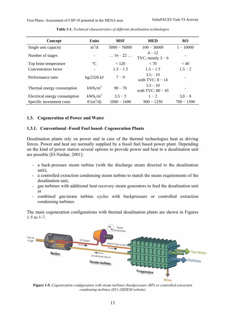
1.3.1. Conventional -Fossil Fuel based- Cogeneration Plants
Desalination plants rely on power and in case of the thermal technologies heat as driving
forces. Power and heat are normally supplied by a fossil fuel based power plant. Depending
on the kind of power station several options to provide power and heat to a desalination unit
are possible [El-Nashar, 2001]:
- a back-pressure steam turbine (with the discharge steam directed to the desalination
unit),
- a controlled extraction condensing steam turbine to match the steam requirements of the
desalination unit,
- gas turbines with additional heat recovery steam generators to feed the desalination unit
or
- combined gas/steam turbine cycles with backpressure or controlled extraction
condensing turbines.
The main cogeneration configurations with thermal desalination plants are shown in Figures
1-5 to 1-7.
Figure 1-5. Cogeneration configuration with steam turbines (backpressure (BP) or controlled extraction
condensing turbines (EC) (SIDEM website)
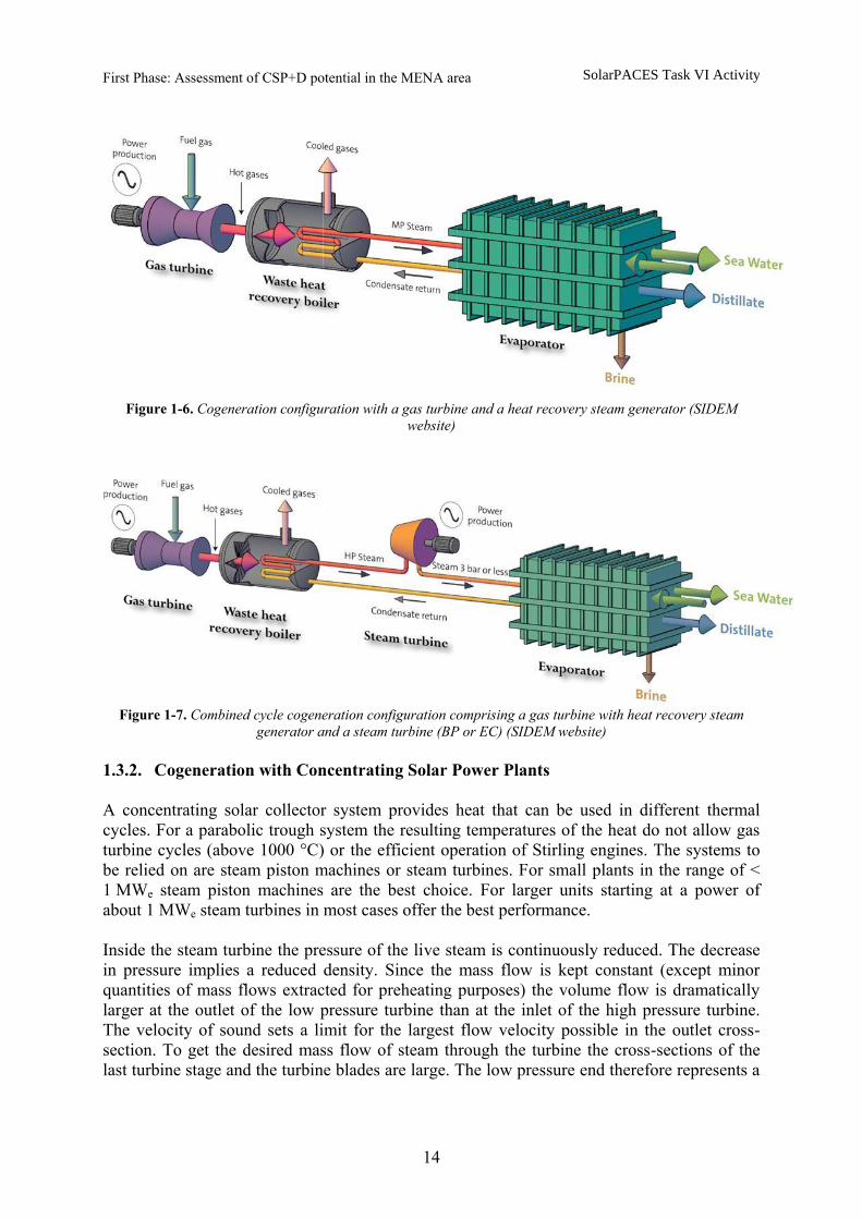
First Phase: Assessment of CSP+D potential in the MENA area SolarPACES Task VI Activity
14
Figure 1-6. Cogeneration configuration with a gas turbine and a heat recovery steam generator (SIDEM
website)
Figure 1-7. Combined cycle cogeneration configuration comprising a gas turbine with heat recovery steam
generator and a steam turbine (BP or EC) (SIDEM website)
1.3.2. Cogeneration with Concentrating Solar Power Plants
A concentrating solar collector system provides heat that can be used in different thermal
cycles. For a parabolic trough system the resulting temperatures of the heat do not allow gas
turbine cycles (above 1000 °C) or the efficient operation of Stirling engines. The systems to
be relied on are steam piston machines or steam turbines. For small plants in the range of <
1 MWe steam piston machines are the best choice. For larger units starting at a power of
about 1 MWe steam turbines in most cases offer the best performance.
Inside the steam turbine the pressure of the live steam is continuously reduced. The decrease
in pressure implies a reduced density. Since the mass flow is kept constant (except minor
quantities of mass flows extracted for preheating purposes) the volume flow is dramatically
larger at the outlet of the low pressure turbine than at the inlet of the high pressure turbine.
The velocity of sound sets a limit for the largest flow velocity possible in the outlet cross-
section. To get the desired mass flow of steam through the turbine the cross-sections of the
last turbine stage and the turbine blades are large. The low pressure end therefore represents a

First Phase: Assessment of CSP+D potential in the MENA area SolarPACES Task VI Activity
15
significant fraction of the investment costs. The smaller the pressure at the outlet, the larger is
the required turbine cross-section.
Figure 1-8. Sketch of a condensation turbine (Toshiba website)
Turbines can be divided into the so called condensation turbines and back-pressure turbines.
For condensation turbines the pressure at the outlet is kept on a very small level by means of a
condenser. These turbines are designed for pure electricity production. From the
thermodynamic view the enthalpy difference useable for conversion into mechanical energy is
higher the lower the outlet pressure is. End stages of condensation turbines are large due to
the low pressure, see Figure 1-8. Back-pressure turbines are used for co-generation of
electricity and heat. The pressure at the outlet is higher than in condensation turbines. The
thermal energy not used for expansion in the turbine is used as a heat source for various
purposes. This can be, e.g., a direct feed-in into an industrial process heat network or the use
in a municipal heating net or, of course, used to feed in a thermal desalination unit. Cross-
sections of this type of turbine are smaller and the turbine itself is cheaper since the cost-
intensive low-pressure stages are not required, see Figure 1-9.
Figure 1-9. Sketch of a back-pressure turbine (Toshiba website)
When designing a turbine system the first boundary condition to be defined is the desired
pressure level at the outlet of the turbine. Although the back-pressure of a turbine can be
varied during operation these variations have to be kept within narrow ranges. Otherwise the

First Phase: Assessment of CSP+D potential in the MENA area SolarPACES Task VI Activity
16
turbine efficiency and/or the power will significantly decrease. Transferred to the CSP+D
system this means that a turbine applied to such a system cannot be used as a condensation
turbine and back-pressure turbine in parallel. The operation of a desalination unit with waste
heat steam requires a back-pressure turbine with a (nearly) constant pressure level.
An alternative to using the steam leaving the last turbine stage is to extract a portion of steam
between one of the up-stream turbine stages. This turbine is called a condensation turbine
with steam extraction. Having the steam extraction point located between two stages the
pressure level of the steam at this stage changes with the load of the turbine. The relation
between steam mass flow/turbine power and extraction pressure is nearly linear. For a solar
thermal power plant operating in a wide range of load points a constant pressure for driving a
thermal desalination process cannot be realized.
To stabilize the extraction pressure a so called controlled extraction can be used. The steam is
taken from different extraction points (pressure levels). Depending on the actual load the
portion of the participating extraction points is automatically controlled. This construction
allows a constant pressure level of the extracted steam but requires a throttling and therefore a
loss of useable energy in certain load points. Due to the constructional effort these turbines
are more expensive than turbines with fixed extraction points.
For a combined CSP and Desalination plant there are two turbine configurations possible:
- a pure back-pressure turbine
- a condensation turbine with controlled extractions.
For a system with a high fresh water production capacity the first option will be the best
choice since the full amount of waste steam from the turbine can be used in the desalination
system at every time. If the purpose of the plant is electricity generation and only a small
desalination unit has to be fed the second option is the best choice since the steam not sent to
the desalination plant can efficiently be used in the last stages of the turbine.
2. Solar resource assessment in the Egypt coastal strip
2.1. Introduction and context
Solar radiation is a climatic variable measured only in few meteorological stations and during
short and, on most occasions, discontinuous periods of time. Therefore, developers do not
find appropriate historical databases with information available on solar resource for specific
sites. Different approaches are available to characterize the solar resource of a specific site.
The possible options are:
Approximation by using data from nearby stations. This option can be useful for
relatively flat terrains and for distances of less than 10 km from the site. In the case of
complex terrain or longer distances, the use of radiation data from other geographical
points is inappropriate.
Interpolation of surrounding measurements. This approach can be used only for areas
with a grid of measurement stations and for average distances between the stations of
about 20-50 km [Pérez et al., 1997; Zelenka et al., 1999].

First Phase: Assessment of CSP+D potential in the MENA area SolarPACES Task VI Activity
17
Solar radiation estimation from satellite images is currently the most suitable
approach. It supplies the best information on the spatial distribution of the solar
radiation and it is a methodology broadly accepted by the scientific community and
with a high degree of maturity [McArthur, 1998]. In this regard, it is worth to mention
that BSRN (Baseline Surface Radiation Network) has among its objectives the
improvement of methods for deriving solar radiation from satellite images, and also
the Experts Working Group of Task 36 of the Solar Heating and Cooling Implement
Agreement of IEA (International Energy Agency) focuses on solar radiation
knowledge from satellite images. Nevertheless it is mandatory to have at least one
reference weather station in the area to calibrate the satellite data.
In this work, an assessment has been done to estimate the solar resource potential in the Egypt
coastal strip using satellite images (Irsolav, Spain). Yearly sums of global horizontal (GHI)
and direct normal irradiance (DNI) are calculated in all the Egypt coastal strip distributed with
a mean distance of 5 km from the sea and separated between each other with a spatial
resolution of 5 km.
2.2. Definition of geographical locations for the solar resource assessment
The assessment of the geographical coordinates of the points along the Egyptian coastal strip
has been done with Google Earth software [Google, 2011]. Figure 2-1 shows the
Mediterranean Sea coastal strip and Figure 2-2 the elevation profile of the Mediterranean Sea
coastal line selected. Figure 2-3 shows the Red Sea coastal strip and Figure 2-4 the elevation
profile for the set of points selected on this coast.
Figure 2-1. Egypt coastal strip at the Mediterranean Sea in red colour (drawn by Google Earth)
Figure 2-2. Elevation profile of the Egypt coastal strip at the Mediterranean Sea

First Phase: Assessment of CSP+D potential in the MENA area SolarPACES Task VI Activity
18
Figure 2-3. Egypt coastal strip at the Red Sea, the red line inland corresponds to the Egypt border drawn by
Google Earth
Figure 2-4. Elevation profile of the Egypt coastal strip at the Red Sea
2.3. Methodology for solar radiation derived from satellite images
Solar radiation calculated from satellite images is based upon the establishment of a
functional relationship between the solar irradiance at the Earth’s ground surface and the
cloud index estimated from satellite images. This relationship has been previously fitted using
high quality ground data, in such a manner that the solar irradiance-cloud index correlation
can be extrapolated to any location of interest. This way, solar radiation components (global,
diffuse and direct) can be calculated from satellite observations.
Following the methodology developed under European Union R&D projects [Rigollier et al.,
2000a; Meyer et al., 2004; Rigollier et al., 2004] IrSOLaV, in collaboration with the group of
Solar Radiation Resource Assessment of the Renewable Energy Division of CIEMAT, has
developed its own methodology to estimate the solar radiation components from Meteosat
First and Second Generation satellite images [Ramírez et al., 2004; Zarzalejo, 2005; Polo et
al., 2006; Polo J. et al., 2008]. However, in this study only satellite images from Meteosat
Second Generation have been used. Even though the different research groups working in this
field are making use of the same core methodologies, there are several characteristics that are
First Phase: Assessment of CSP+D potential in the MENA area SolarPACES Task VI Activity
19
different depending on the specific objectives pursued. The main differences between the
IrSOLaV/CIEMAT and others, like the ones applied by PVGis or Helioclim are:
- Selection of the working window. The correlations developed by IrSOLaV/CIEMAT
are focused on the Iberian Peninsula, and in particular in Spain, making use of 30
equidistant meteo-stations in this territory. However, the other groups use stations
distributed all around Europe and the resulting relationships are applied to any
location.
- Filtering of images and terrestrial data. Images and data used for the fitting and the
establishment of relationships are filtered with procedures developed specifically for
this purpose.
- Selection of albedo for clear sky. The algorithm used for the selection of clear sky
albedos provides a daily sequence that is different for every year. However, the other
methodologies use a unique monthly value.
- Introduction of characteristic variables. The relationship developed by
IrSOLaV/CIEMAT includes new variables characterizing the climatology of the site
and the geographical location, with a significant improvement of the estimations
obtained for global and direct solar radiation.
The quantification of solar irradiation from satellite images is based upon the so called
Heliosat-2 model, which has been modified and assessed at CIEMAT by using 30 ground
stations in Spain. IrSOLaV has developed from the initial Heliosat-2 method a new
operational tool able to be applied to a database of images from 1995 until 2010. However,
images from 2006 to 2010 which belong to Meteosat Second Generation have been used in
this study. The satellite images belong to the high resolution visible channel (HRV) with a
spatial resolution of about 1 x 1 km2. It is worth to note that this tool has been specifically
adapted for the Spanish climatology. The uncertainty of the estimation comparing with hourly
ground pyranometric measurements is expressed in terms of the relative root mean squared
error (RMSE).
Different assessments and benchmarking tests can be found at the available literature
concerning the use of satellite images (Meteosat and GOES) on different geographic sites and
using different models [Pinker and Ewing, 1985; Zelenka et al., 1999; Pereira et al., 2003;
Rigollier et al., 2004; Lefevre et al., 2007]. The uncertainty for hourly values is around 20 -
25% RMSE and on a daily basis the uncertainty of the models is about 13-17% in terms of
RMSE. It is important to note that Zelenka concluded that among the sources of the error,
between 12-13% is due to the methodology itself (conversion of satellite digital level
information into radiation data) and a relevant fraction of 7-10% is due to the uncertainty of
the ground measurements used for the comparison. In addition, Zelenka estimates that the
error of using nearby ground radiometric stations beyond 5 km reaches 15% in terms of
RMSE. For that reason, his conclusion is that the use of hourly radiometric data derived from
satellite images is more accurate than ground measurements from nearby stations located
more than 5 km far from the site of analysis. IrSOLaV methodology to estimate solar
radiation from satellite images is based on the work developed by the group of Solar
Radiation Resources Assessments of CIEMAT [Zarzalejo et al., 2007]. The model has been
assessed for about 30 Spanish sites with the following uncertainty data for global horizontal
irradiance:
- About 15% RMSE for hourly values.

First Phase: Assessment of CSP+D potential in the MENA area SolarPACES Task VI Activity
20
- Less than 10% for daily values.
- Less than 5% for annual and monthly means.
The model described in Zarzalejo et al. (2007), has been modified for a better estimation of
solar radiation with clear sky, leading to an important improvement in the accuracy of the
model [Polo, 2009; Polo et al., 2009b]. The estimation of direct normal radiation has been
done using a new database of Aerosol optical depth (AOD 550nm), and Linke turbidity
climatology with a spatial resolution of 1/12º developed in IEA SHC Task 36 has been used
[Remund et al., 2010]. This database has been calculated using merging MODIS and MSIR
satellite data and ground measurements from Aeronet network sites. Further corrections for
the coherence with Meteonorm database have been applied.
2.4. Results and comments
Solar radiation has been estimated for the pixels of the satellite images which correspond to a
series of sites separated by a distance of 5 km and following Egypt’s coastal strip. In general
terms, the dynamic of yearly solar radiation can be divided into two main zones.
Figure 2-5. DNI results of the Egypt coastal strip at the Mediterranean sea
The Mediterranean Sea Zone. Figure 2-5 shows the yearly DNI results for each site
(corresponding to the map shown below). The range oscillation is from 1,854 to 2,247 kWh
m-2
year-1
.The mean values of the DNI for sites corresponding to longitudes between 30 and
32ºE are lower than the rest. This is due to the fact that this zone belongs to the delta of the
Direct Normal Radiation on the Mediterranean Coast
1800
1900
2000
2100
2200
2300
2400
2500
2600
25,08 26,08 27,08 28,08 29,08 30,08 31,08 32,08 33,08 34,08
Longitude (ºE)
Ra
dia
tio
n (
W/m
^2
)

First Phase: Assessment of CSP+D potential in the MENA area SolarPACES Task VI Activity
21
Nile River, with a different land cover and there is big content of water vapour in the
atmosphere.
The Red Sea Zone. Figure 2-6 shows the yearly DNI results for west side of the Red sea.
Overall, the DNI values show higher mean values than the results for the Mediterranean zone.
The minimum value is 2,245 and the maximum 2,551 kWh m-2
year-1
. In this zone, there is
higher variability than in the Mediterranean coast due to the abruptness of the terrain.
Figure 2-6. DNI results of the Egypt coastal strip in the west side of the Red sea
The closeness of the sea doesn’t have any effect on the ground albedo of the sites evaluated,
and therefore in the values of DNI estimated, due to the spatial resolution of the pixel of the
satellite images and the distance from the sea. However, the arid soil cover (inland or
coastline) can have an effect on the values of DNI estimated from satellite. In Egypt, the
terrain is highly reflecting and can have an effect on the estimations of the model achieving a
lower precision and a sub-estimation of solar radiation (for both global and especially DNI).
This effect is due to the fact that high reflectance is associated with cloudy conditions.
Direct Normal Radiation on the west of the coast of the Red Sea coast
1800
1900
2000
2100
2200
2300
2400
2500
2600
22,0123,0124,0125,0126,0127,0128,01
Latitude (ºN)
Ra
dia
tio
n (
W/m
^2
)

First Phase: Assessment of CSP+D potential in the MENA area SolarPACES Task VI Activity
22
3. Feasible configuration options to CSP+D cogeneration plants
3.1. Introduction
The objective of this project is the realization of a technical assessment of the potential of
Concentrating Solar Power plants with Desalination (CSP+D) facilities in the MENA (Middle
East and North African) area. The project has been divided into two phases, the first one
consisting in the assessment of possible configurations of CSP+D to optimize the production
of water and electricity within the MENA region, and the second one consisting in a
feasibility study of CSP+D integrated plant in Port Safaga. For this proposal, different
configurations for electricity and water production have been simulated and compared to each
other. The CSP plant consists of a parabolic trough (PT) power plant based on Reheat cycle
with feedwater heaters, using water as the working fluid. The desalination technologies
considered for the combination with the PT-CSP plant are multi-effect distillation (MED) and
reverse osmosis (RO).
Two MED configurations have been taken into account: a low temperature multi-effect
distillation (LT-MED) unit using the exhausted steam from the CSP plant as the source of
heat, and a low temperature multi-effect distillation plant powered by the steam obtained from
a thermal vapour compressor (TVC). In this case, unlike the conventional thermal vapour
compression MED process (TVC-MED), the entrained vapour to be used in the steam ejector
comes from the exhausted steam of the CSP plant instead of an intermediate effect of the
distillation unit. Within the latter concept (LT-MED-TVC), different schemes have been
studied: one using the high exergy steam from the high pressure turbine outlet as motive
steam in the TVC, and others using steam extracted at different pressures from the low
pressure turbine as the motive steam in the ejector. In all studied cases, the freshwater and
electricity production considered are the same (35,018 m3/day and 50 MWe, respectively).
The results obtained are valid for arid regions, where RO has higher specific electric
consumption and dry cooling is used in CSP plants.
3.2. Description of the systems
The systems under consideration are (Figure 3-1 to Figure 3-3):
- Configuration 1: LT-MED unit integrated into a parabolic through concentrating solar
power (PT-CSP) plant (Figure 3-1).
- Configuration 2: LT-MED-TVC unit integrated into a PT-CSP plant (Figure 3-2).
- Configuration 3: RO unit connected to a PT-CSP plant (Figure 3-3).
The CSP plant consists of a large field of single-axis parabolic-trough solar collectors (LS3
type) aligned on a north-south orientation and a thermal storage tank to provide additional
operation when solar radiation is not available. The collectors track the sun from east to west
during the day to ensure it is continuously focused on the linear receiver. The cycle is a
conventional, single reheat design with closed feedwater heaters. In the case of
configuration 1, the cycle has four closed feedwater heaters instead of five (like in the case of
configurations 2 and 3), since the lowest pressure steam extraction is not used. In this case
steam extracted at 0.3121 bar (70 ºC) is used to feed the desalination plant, which decreases
the power production efficiency with respect to the rest of cases where the condensing

First Phase: Assessment of CSP+D potential in the MENA area SolarPACES Task VI Activity
23
temperature is slightly lower. Also, the cycle has a deaerator to remove the air and other
dissolved gases from the feedwater. A dry cooling system is considered for condensing the
exhaust steam from the turbine in the power block, which is the usual means in arid areas,
since the typical wet cooling towers consume between 2 and 3 metric tons per MWh [Richter
and Dersch, 2009].
As it can be observed in the mentioned figures, in all configurations, the thermal energy from
the solar field is exploited by a power conversion system consisting of a pre-heater, an
evaporator and a superheater. The resulting superheated steam at point 1 is sent to a high
pressure turbine (ST1) where, after suffering an expansion process, is extracted at point 2 to
preheat feedwater in one closed feedwater heater (FWH1). The steam that leaves the high
pressure turbine at 3 is routed through a reheater, where it is superheated up to 4. The reheated
steam is left to its expansion through a low pressure (ST2) turbine up to 13 in the first
configuration and 10 in the rest, producing power. Four steam extractions are taken from the
low pressure turbine in the case of configuration 1: one is directed to the deaerator and the
remaining three to feedwater heaters (FWH1-4).
In the case of configurations 2 and 3, five extractions are taken from the low pressure turbine:
one is directed to the deaerator and the rest to feedwater heaters (FWH1-5). The steam leaving
the low pressure turbine is condensed through the LT-MED heat exchanger in
configuration 1, and through a dry condenser in the rest. The condensed steam (feedwater) is
pumped to a sufficiently high pressure (8.38 bar) to allow it to pass through the two low
pressure feedwater heaters in the case of configuration 1, through three low pressure
feedwater heaters in the case of configurations 2 and 3, and into the deaerator. The feedwater
is pumped again at the outlet of the deaerator to a pressure slightly higher than the boiling
pressure in the preheater (103 bar). Feedwater passes through the two high pressure feedwater
heaters before returning to the preheater in order to complete the cycle.
The configuration showed in Figure 3-1 consists of a low-temperature multi-effect distillation
(LT-MED) unit integrated into a parabolic-trough concentrating solar power (PT-CSP) plant.
In this option, the desalination plant is fed at 13 by the low temperature steam from the
turbine outlet (0.3121 bar, 70 ºC).
Figure 3-1. Diagram of the LT-MED unit integration into a PT-CSP plant
In the second configuration, two options are considered: one using the high exergy steam
from the high pressure turbine (ST1) outlet at 11 as motive steam in the steam ejector, and
ST1
Reheater
Preheater
Evaporator
Superheater
Closed
FWH 1
1
2
3
4
Closed
FWH 2Deaerator
5
6
ST2
7
Closed
FWH 3
8
Closed
FWH 4
13
Pump 2 Pump 1
LT-MED
Fresh water
Thermal
Storage
Solar field1415
First Phase: Assessment of CSP+D potential in the MENA area SolarPACES Task VI Activity
24
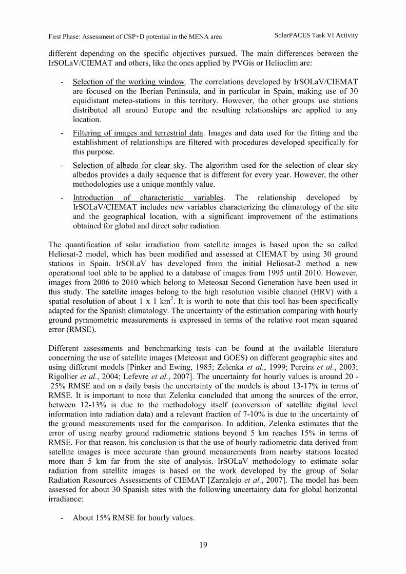
others using steam extracted at 5, 6, 7 and 8 from the low pressure turbine (ST2) as the motive
steam in the ejector. Moreover, one part of the exhausted steam from the turbine at 12 is used
as entrained vapour in the ejector. Then, the resulting compressed vapour from the ejector is
injected into the first effect of the distillation unit at 13. Figure 3-2 shows the cases (a) in
which one part of the steam that leaves the high pressure turbine and (b) one part of the steam
that is extracted from the low pressure turbine at 11 is used as motive steam, respectively.
(a)
(b)
Figure 3-2. Diagram of the LT-MED-TVC unit integration into a PT-CSP plant. (a) The steam is
extracted from the HP turbine (b) The steam is extracted from LP turbine
Finally, in the configuration 3 (see Figure 3-3), the RO plant is driven by the power output
from the PT-CSP plant.
Figure 3-3. Diagram of the RO unit integration into a PT-CSP plant
ST1
Reheater
Preheater
Evaporator
Superheater
Closed
FWH 1
1
2
3
4
Closed
FWH 2Deaerator
ST2
5
Closed
FWH 3
6
Closed
FWH 4
7
Pump 2
Pump 1
LT-MED
Fresh waterClosed
FWH 5
Dry cooling
8 9
10
11
12
Thermal
Storage
Solar field
13
1415
ST1
Reheater
Preheater
Evaporator
Superheater
Closed
FWH 1
1
2
3
4
Closed
FWH 2Deaerator15
5
6
ST2
Closed
FWH 3Closed
FWH 4
7
14Pump 2
Pump 1
LT-MED
Fresh waterClosed
FWH 5
Dry cooling
8
11
10
12
13
9
Solar field
Thermal
Storage
ST1
Reheater
Preheater
Evaporator
Superheater
Closed
FWH 1
1
2
3
4
Closed
FWH 2Deaerator
5
6
ST2
7
Closed
FWH 3
8
Closed
FWH 4
9
Fresh water
Pump 2 Pump 1Closed
FWH 5
ROHigh pressure
pump
Dry cooling
10
Thermal
Storage
Solar field 1415

First Phase: Assessment of CSP+D potential in the MENA area SolarPACES Task VI Activity
25
Table 3-1 shows the operating conditions and assumptions that have been used in the
thermodynamic simulation, which are based in the data published for the Andasol 1 plant
[Blanco-Marigorta et al., 2011]. The turbine inlet parameters (373 °C, 100 bar) are the typical
values of the Andasol power plants. The temperature level is lower than in conventional
Rankine cycles, since the heat transfer fluid (HTF) temperature from the solar field is limited
to 390 °C due to stability reasons. For such pressure and temperature turbine inlet values,
steam reheating is required not only for increasing the power generation but also for avoiding
large end moisture fraction (which is to be typically kept below 10-12 % [Strauß, 2006]).
Table 3-1. Operating conditions and assumptions used in the thermodynamic simulation of analyzed
configurations 1, 2 and 3
Point in the diagram Magnitude Value
1 Pressure and
temperature 373ºC, 100 bar
2 Pressure 33.5 bar
3 Pressure 18.50 bar
4 Pressure and
temperature 373.4ºC, 16.50 bar
5 Pressure 14 bar
6 Pressure 6.18 bar
7 Pressure 3.04
8 Pressure 1.17 bar
9 Pressure 0.37 bar
10 Pressure 0.18 bar
12 Pressure 0.18 bar
13 Pressure 0.31 bar
14 Pressure 8.38 bar
15 Pressure 103 bar
TTD Temperature 4ºC
DCA Temperature 5ºC
ΔPRH Pressure 2 bar
ΔPWL Pressure 0.5/0.1 bar
ΔPST Pressure 0.1 bar
Where:
TTD = Terminal temperature difference in feedwater heaters, in ºC,
DCA = Drain cooler approach in feedwater heaters, in ºC,
ΔPRH = Pressure losses in the reheater, in bar,
ΔPWL = Pressure losses in the water lines HP/LP feedwater heaters, in bar, and
ΔPST = Pressure losses in the steam lines, in bar.
The TTD (terminal temperature difference) is the difference between saturation temperature at
the extraction pressure and the water temperature at the heater outlet. The DCA (drain cooling
approach) is the difference between the cold water at the heater inlet and the sub-cooled steam
at the heater outlet. For these calculations, nominal values adopted for TTD and DCA are
5 °C and 4 °C, respectively [Blanco-Marigorta, 2011]. Regarding the pressure losses in the re-
heater and in the water/steam lines, typical values of the Andasol plants have been chosen
[Blanco-Marigorta, 2011].

First Phase: Assessment of CSP+D potential in the MENA area SolarPACES Task VI Activity
26
In all cases, a CSP plant net power production of 50 MWe has been considered since this is a
typical size of these plants nowadays [Geyer et al., 2006]. The capacity of the desalination
plants is 35,018 m3/day, which has been determined by the analysis of the first configuration
(PT-CSP + LT-MED). As explained above, in this configuration all the steam from the solar
power plant (see Figure 3-1, point 13) is used as the heat transfer media in the desalination
unit, producing fresh water. As can be observed in Table 2, another common condition for
configurations 2 and 3 is that the steam is allowed to be expanded up to 58ºC (0.18 bar). This
is the result of the use of dry condensers that has been chosen as a feasible option for solar
power plants in these arid regions [Hamed et al., 2006].
3.3. Analysis of the systems
The work was structured in several subtasks, as can be seen in Figure 3-4. Firstly, the steam
condensation temperature in the power block needs to be known. Then, the procedure consists
of an iterative calculation of the size of steam turbine and solar field in order to meet the
required net power generation at design conditions. The iteration is required since the internal
electricity consumption of the various plant components (solar field, thermal energy storage,
steam turbine, cooling block and desalination) are dependent on the components’ capacity,
which are still not known at the beginning of the calculation.
The net power generation results from the gross power production minus the sum of the
internal power consumption (parasitics) of the plant components:
1i
N
net gross parasitics
i
P P P
(1)
where
Pnet is the net power generation, in MW,
Pgross is the gross power generation, in MW, and
Pparasitics, the internal power consumptions of plant components, in MW.
These parasitics correspond to the power consumption by: the solar field, the thermal storage,
the steam turbine, the cooling systems and the desalination plant.
The thermodynamic analysis has been performed by implementing a computer model in
Engineering Equation Solver (EES) software. The steady-state model has been made by
proposing a set of nonlinear, algebraic equations for each thermodynamic cycle. All the
components associated with the power cycle (pump, reheater, heat exchanger, condenser and
turbine) are analyzed by steady-flow energy equations. In this phase of the project, only the
parasitics corresponding to the steam turbine, the cooling system and the desalination plant
have been considered.
The calculation is firstly performed for the configuration PT-CSP+LT-MED, which allows
defining the net water production for the rest of cases. In all the analyzed configurations, the
net water production is slightly less than the gross one, since a part of the water produced is
consumed internally in the power plant for cleaning the mirrors, for the power block water
supply and other consumptions (drinking water).

First Phase: Assessment of CSP+D potential in the MENA area SolarPACES Task VI Activity
27
Figure 3-4. Simplified calculation scheme
To carry out the assessment, the following assumptions have been taken into account:
- Actual expansion and compression processes have been considered.
- An isentropic efficiency of 0.852 has been taken for the high pressure steam turbine,
and an isentropic efficiency of 0.85 for the low pressure steam turbine.
- An isentropic efficiency of 0.75 has been taken for the pumps of the power cycle.
- A specific electric consumption of 2.11 kWh/m3 has been assumed in the case of
MED plant and 5.46 kWh/m3 in the case of RO, which are the estimated values for
Egypt [Trieb, 2007].
- The GOR (Gained Output Ratio) has been assumed to be 8.4 in all cases of MED
plant. It is defined as kilograms of distillate produced for every kilogram of steam
supplied to the system.
- The power required by the cooling unit has been taken from a study of a dry-cooled
parabolic trough plant located in the Mojave Desert, which showed 5% less electric
energy produced annually [Richter and Dersch, 2010]. In configuration 2, since not all
First Phase: Assessment of CSP+D potential in the MENA area SolarPACES Task VI Activity
28
the steam is driven to the condenser, the energy consumption due to the dry cooling is
proportionally lower.
The solar field size has been determined by a computer model developed in MATLAB taking
into account thermal losses, efficiency and energy balances. The parabolic trough solar field is
based on the LS-3 type collector, which has the following features:
Table 3-2. LS-3 collector characteristics
Magnitude Units Value
Absorber diameter (int/ext) mm 65/70
Geometric concentration - 26
Longitude m 99
Aperture area m² 545
Maximum working temperature ºC 390
Distance between parallel rows m 17
Peak optical efficiency - 0.76
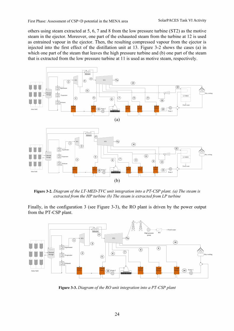
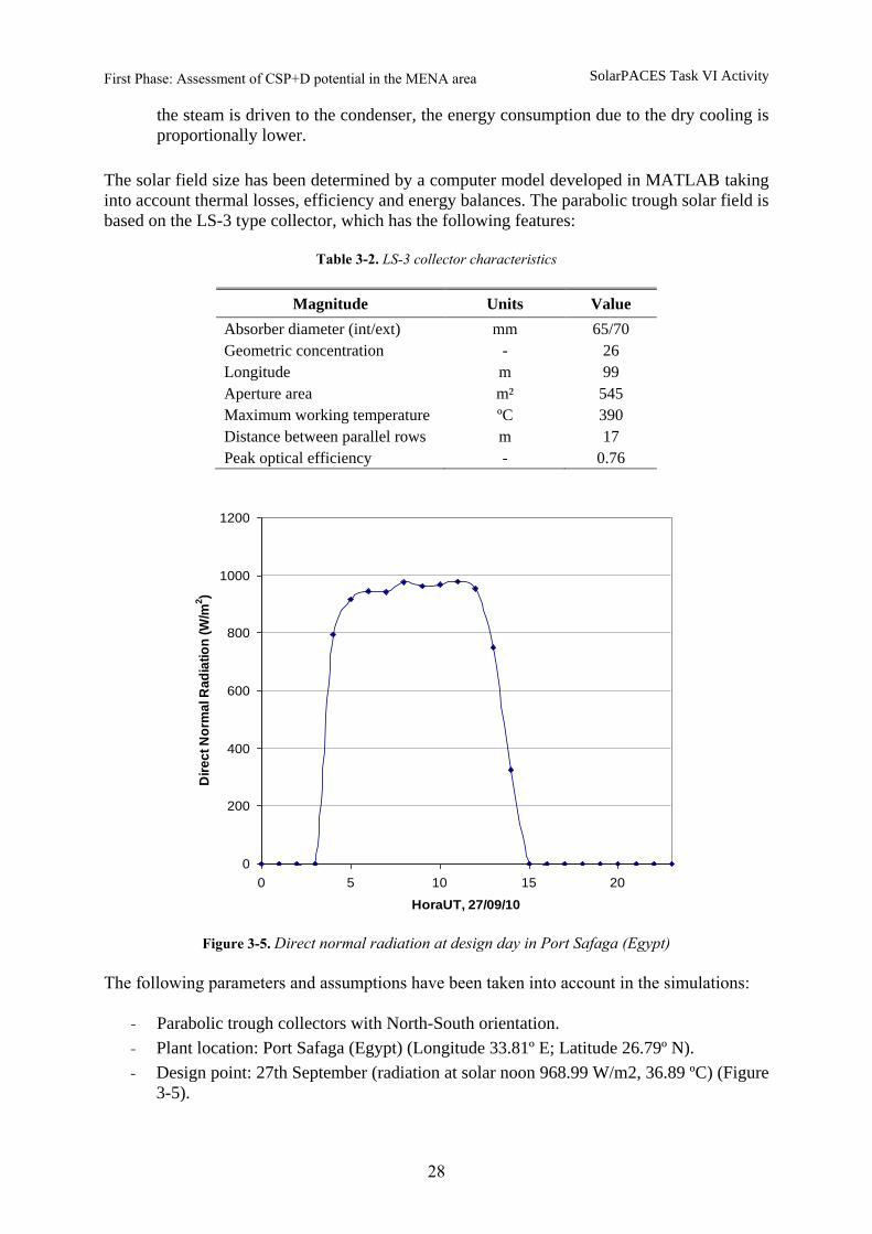
Figure 3-5. Direct normal radiation at design day in Port Safaga (Egypt)
The following parameters and assumptions have been taken into account in the simulations:
- Parabolic trough collectors with North-South orientation.
- Plant location: Port Safaga (Egypt) (Longitude 33.81º E; Latitude 26.79º N).
- Design point: 27th September (radiation at solar noon 968.99 W/m2, 36.89 ºC) (Figure
3-5).
0
200
400
600
800
1000
1200
0 5 10 15 20
HoraUT, 27/09/10
Dir
ec
t N
orm
al R
ad
iati
on
(W
/m2)
First Phase: Assessment of CSP+D potential in the MENA area SolarPACES Task VI Activity
29
- Thermal storage capacity for roughly 23-h solar operation at design day (taking into
account 9% of thermal losses).
- The net output thermal capacity calculated before.
- Inlet temperature to the field: 295 °C.
- Outlet temperature from the field: 390 °C.
The simulations were carried out for Port Safaga, in Egypt. With about 2,496 kWh/(m2·yr)
DNI radiation, this site represents a good location for CSP plants in the MENA area.
Radiation and ambient temperature data have been taken from a meteorological year type data
set generated with Meteonorm (monthly horizontal global irradiance data, ambient
temperature and wind velocity obtained from NASA-SEE). The DNI data have been
normalized with the satellite measurement of the annual average of the DNI provided by the
company IRSOLAV. The oil type is Monsanto VP-1 (its properties are determined using
Monsanto software).
3.4. Economic analysis
The economic analysis has been carried out by the assessment of the power and water costs of
the configurations proposed. On one hand, the power cost has been determined by the
Levelized Electricity Cost (LEC), which is defined as [Short et al., 1995]:
&invest O M fuel
net
crf K K KLEC
E
(2)
Crf is the capital recovery factor, which is calculated by:
1
1 1
n
d d
insurancen
d
k kcrf k
k
(3)
where
Kinsurance is the annual insurance rate (value used = 1%),
Kinvest is the total investment of the plant,
Kfuel is the annual fuel cost (which is only applicable in the case of solar energy with
backup),
kd (value used = 8%) is the real debt interest rate, n is the depreciation period in years
(value used = 25 years),
KO&M are the annual operation and maintenance costs and
Enet is the annual net electricity delivered to the grid.
Additional data used to calculate the cost of the solar power are the following:
First Phase: Assessment of CSP+D potential in the MENA area SolarPACES Task VI Activity
30
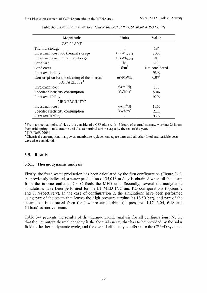
Table 3-3. Assumptions made to calculate the cost of the CSP plant & RO facility
Magnitude Units Value
CSP PLANT
Thermal storage h 13♠
Investment cost w/o thermal storage €/kWnominal 3300
Investment cost of thermal storage €/kWhstored 40
Land size ha 200
Land costs €/m2 Not considered
Plant availability - 96%
Consumption for the cleaning of the mirrors m3/MWhe 0.07♣
RO FACILITY♦
Investment cost €/(m3/d) 850
Specific electricity consumption kWh/m3 5.46
Plant availability - 92%
MED FACILITY♦
Investment cost €/(m3/d) 1050
Specific electricity consumption kWh/m3 2.11
Plant availability - 98%
♠ From a practical point of view, it is considered a CSP plant with 13 hours of thermal storage, working 23 hours
from mid-spring to mid-autumn and also at nominal turbine capacity the rest of the year. ♣ [US DoE, 2009] ♦ Chemical consumption, manpower, membrane replacement, spare parts and all other fixed and variable costs
were also considered.
3.5. Results
3.5.1. Thermodynamic analysis
Firstly, the fresh water production has been calculated by the first configuration (Figure 3-1).
As previously indicated, a water production of 35,018 m3/day is obtained when all the steam
from the turbine outlet at 70 ºC feeds the MED unit. Secondly, several thermodynamic
simulations have been performed for the LT-MED-TVC and RO configurations (options 2
and 3, respectively). In the case of configuration 2, the simulations have been performed
using part of the steam that leaves the high pressure turbine (at 18.50 bar), and part of the
steam that is extracted from the low pressure turbine (at pressures 1.17, 3.04, 6.18 and
14 bars) as motive steam.
Table 3-4 presents the results of the thermodynamic analysis for all configurations. Notice
that the net output thermal capacity is the thermal energy that has to be provided by the solar
field to the thermodynamic cycle, and the overall efficiency is referred to the CSP+D system.

First Phase: Assessment of CSP+D potential in the MENA area SolarPACES Task VI Activity
31
Table 3-4. Net Output Thermal Capacity (NOTC), overall efficiency, cooling requirements, number of collector
per row, number of rows, aperture area resulting from each diagram proposed
Desalination system NOTC
(MWth)
Overall
efficiency
(%)
Cooling
requirements
(%)
Number of
collectors per
row
Number of
rows
Aperture
area (m2)
LT-MED 161 31.1 0 2 673 733,570
LT-MED-TVC
(1.17 bar) 180 27.7 19 2 756 824,040
LT-MED-TVC
(3.04 bar) 191 26.2 27 2 800 872,000
LT-MED-TVC
(6.18 bar) 198 25.2 30 2 831 905,790
LT-MED-TVC
(14 bar) 208 24.1 34 2 870 948,300
LT-MED-TVC
(18.5 bar) 199 25.2 35 2 832 906,880
RO 175 28.6 100 2 733 798,970
On one hand, it can be observed that the integration of a LT-MED unit into a PT-CSP plant
(first configuration) gets the best results (lowest NOTC, largest overall efficiency and a
smallest solar field). In other words, the decrease in the efficiency of the power production for
this configuration due to the higher pressure of the exhaust steam is less than the extra power
that the CSP must generate in configuration 3 for RO desalination process. However, the main
advantage of the first configuration is that, in this layout, no power cooling is required and
therefore any condenser would be necessary. It leads to conclude that LT-MED could
theoretically be more efficient (from the thermodynamic point of view) than RO in the
MENA region, as opposed to other regions where wet cooling is used and RO desalination
plants have a lower consumption [Moser et al., 2010].
On the other hand, LT-MED-TVC configuration (option 2) shows worse results than
configurations 1 and 3, as it uses a high exergy steam to feed a steam ejector, which provides
the heat transfer media for the desalination process. However, it has an advantage over the RO
configuration (option 3) since the former requires a lower power plant cooling than the latter.
Moreover, comparing the second configuration to the first one, the integration of a LT-MED
into a PT-CSP plant by replacing the cooling unit has a major disadvantage by the fact that
the desalination plant must be very close to the turbine, since the exhaust steam has very low
density and therefore pipes with very large diameters are needed to conduct the steam to the
desalination plant. This is why the thermal compression of the steam (LT-MED-TVC) is also
considered as one option (Configuration 2). In addition to this, this configuration has a huge
interest due to its flexibility for the coupling of any thermal desalination process to a power
plant and not only a MED process.
Taking into account the steam conditions of the configuration 2 pointed out in Table 3-1,
simulations of this option have been carried out. The results obtained have been compared to
the results of the RO configuration analysis (Table 3-4). They are represented in Figs. 3-6 to
3-9.

First Phase: Assessment of CSP+D potential in the MENA area SolarPACES Task VI Activity
32
Figure 3-6. Comparison of the thermal power
obtained in configuration 2 (for every steam extracted
pressure) to the one obtained in configuration 3
Figure 3-7. Comparison of the overall efficiency
obtained in configuration 2 (for every steam
extracted pressure) to the one obtained in
configuration 3
Figure 3-8. Comparison of the thermal power
dissipated in the condenser in conf. 2 (for every steam
extracted pressure) to the one obtained in
configuration 3
Figure 3-9. Comparison between the solar field in
configuration 2 (for every steam extracted pressure)
to the one obtained in configuration 3
The Net Output Thermal Capacity required and the aperture area increase with the pressure of
the steam extracted from the ST2 turbine (Figure 3-6 and Figure 3-9 respectively). Also, the
lower the pressure of the steam is, the larger the overall efficiencies of the system result
(Figure 3-7). Moreover, energy losses to the ambient due to the cooling process of the power
cycle are much lower at all cases in Configuration 2 than in Configuration 3 (Figure 3-8),
although they increase with the pressure of the steam extracted from the turbine.
As it can be observed in Figures 3-6 to 3-9, in the case of extraction from the ST2 turbine at a
pressure of 1.17 bars, Configuration 2 is very similar to Configuration 3 in terms of
efficiency. However, the thermal power dissipated in the condenser is 10 MW, while in
Configuration 3 is 115 MW (see Figure 3-7).
Motive steam and entrained vapor mass flow rates used in Configuration 2 are presented in
Figure 3-10. As it can be observed, the higher the pressure of the motive steam is (steam that
is extracted from the ST2 turbine) the lower the mass flow rate of it is. The trend of the
entrained vapor is just the opposite in order to get a fixed steam flow rate to drive the MED
process.
170
175
180
185
190
195
200
205
210
1.17 6.17 11.17 16.17
Pressure of the steam extracted from the turbine (bar)
NO
TC
(M
W)
LP turbine extractions
Reverse Osmosis
23.5
24
24.5
25
25.5
26
26.5
27
27.5
28
28.5
29
1.17 6.17 11.17 16.17
Pressure of the steam extracted from the turbine (bar)
Ov
era
ll E
ffic
ien
cy
(%
)
LP turbine extractions
Reverse Osmosis
0
20
40
60
80
100
120
140
1.17 6.17 11.17 16.17
Pressure of the steam extracted from the turbine (bar)
Th
erm
al p
ow
er
dis
sip
ate
d in
th
e
co
nd
en
se
r (M
W)
LP turbine extractions
Reverse Osmosis
780000
800000
820000
840000
860000
880000
900000
920000
940000
960000
1,17 6,17 11,17 16,17
Pressure of the steam extracted from the turbine (bar)
Ap
ert
ure
are
a (
m2)
LP turbine extractions
Reverse Osmosis
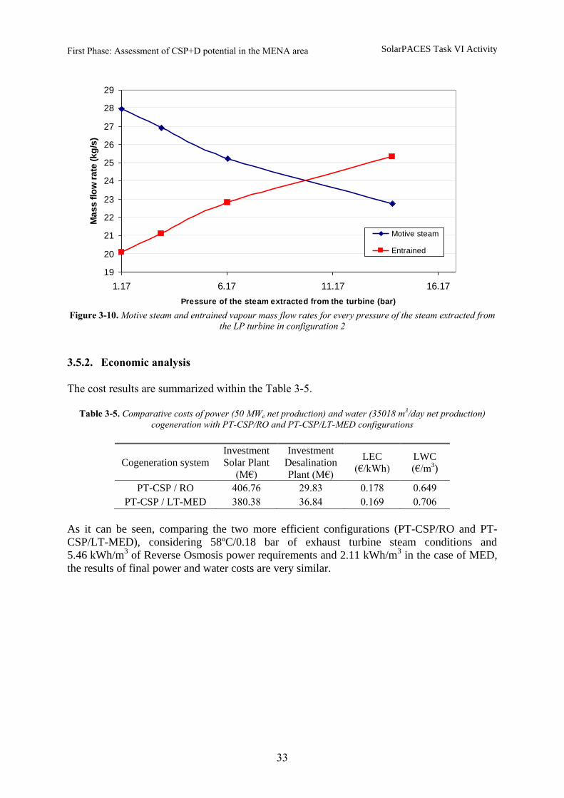
First Phase: Assessment of CSP+D potential in the MENA area SolarPACES Task VI Activity
33
Figure 3-10. Motive steam and entrained vapour mass flow rates for every pressure of the steam extracted from
the LP turbine in configuration 2
3.5.2. Economic analysis
The cost results are summarized within the Table 3-5.
Table 3-5. Comparative costs of power (50 MWe net production) and water (35018 m3/day net production)
cogeneration with PT-CSP/RO and PT-CSP/LT-MED configurations
Cogeneration system
Investment
Solar Plant
(M€)
Investment
Desalination
Plant (M€)
LEC
(€/kWh)
LWC
(€/m3)
PT-CSP / RO 406.76 29.83 0.178 0.649
PT-CSP / LT-MED 380.38 36.84 0.169 0.706
As it can be seen, comparing the two more efficient configurations (PT-CSP/RO and PT-
CSP/LT-MED), considering 58ºC/0.18 bar of exhaust turbine steam conditions and
5.46 kWh/m3 of Reverse Osmosis power requirements and 2.11 kWh/m
3 in the case of MED,
the results of final power and water costs are very similar.
19
20
21
22
23
24
25
26
27
28
29
1.17 6.17 11.17 16.17
Pressure of the steam extracted from the turbine (bar)
Ma
ss
flo
w r
ate
(k
g/s
)
Motive steam
Entrained
vapour
Second Phase: Port Safaga (Egypt) case study SolarPACES Task VI Activity
34
SECOND PHASE
Feasibility study of CSP+D integrated plant in
Port Safaga

Second Phase: Port Safaga (Egypt) case study SolarPACES Task VI Activity
35
4. Feasibility study of CSP+D integrated plant in Port Safaga
The goal of this phase has been the preliminary thermodynamic and –in a further step–
economic analysis and design of a PT-CSP+D plant with an expected net power production at
design conditions of 50 MWe and a 6.5 full load hours of thermal energy storage, which will
be located in Port Safaga. The net water production of the desalination plants is
43,420 m3/day, which has been determined by the analysis of the configuration PT-CSP + LT-
MED. For the analysis, different cooling and desalination options have been analyzed:
Table 4-1. Overview of analyzed configurations
Analysed configurations
1 Once-Through
Reverse Osmosis 2 Evaporative Cooling
3 Dry Cooling
4 LT-MED (Once-through cooled)
The configurations that have been chosen for this analysis have been those ones showed in
Figure 3-1 and Figure 3-3.
4.1. Site location selection
From the assessment of the solar radiation potential in the whole Egyptian coastal strip (see
section 2 within first phase report), the selected location to carry out the study was Port-
Safaga (Fig. 4.1) in the Egyptian Red Sea, about 50 km South of Hurghada and with an
estimated DNI value of 2,496 kWh/m2-yr.
Figure 4-1. Port Safaga geographical coordinates: 26º45’ North, 33º56’ East [Google Earth, 2013]

Second Phase: Port Safaga (Egypt) case study SolarPACES Task VI Activity
36
With relevant industrial and touristic activities, Port Safaga was also considered a good
Middle East representative location. After a visit to the site, two possible sites were initially
selected to the theoretical CSP+D plant location, as indicated in the Figure 4.2.
Figure 4-2. Initial selected locations of the CSP+D cogeneration plant in Port Safaga
Finally, the North Safaga location was selected to carry out the detailed analysis. The site is
located at 2.2 km of distance to the sea, 20 m of altitude above sea level and 8 km north of an
existing electrical substation. Figure 4.3 shows a view of the site.
Figure 4-3. View of final selected location, about 10 km north of Port Safaga

Second Phase: Port Safaga (Egypt) case study SolarPACES Task VI Activity
37
4.2. Analysis of the systems
All considered cases have been designed in order to generate the same amount of net
electricity and water at design conditions. The size of the power block and the solar field was
adapted accordingly case-by-case. It should be highlighted that, within this project phase, it
was not possible to carry out a design optimization. Rather, it was preferred to perform a
preliminary design according to typical design conditions for CSP plants.
The same operating conditions for the CSP plant as those ones showed in Table 3-1 have been
used. The procedure to carry out the thermodynamic analysis has been also the same as the
one showed in Figure 3-4.
The assumptions that have been taken into account in the thermodynamic analysis are the
following ones:
- Actual expansion and compression processes have been considered.
- An isentropic efficiency of 0.86 has been taken for the high pressure steam turbine,
and an isentropic efficiency of 0.85 for the low pressure steam turbine.
- An isentropic efficiency of 0.75 has been taken for the pumps of the power cycle.
- A specific electric consumption of 1.6 kWh/m3 has been assumed in the case of MED
plant and 4.5 kWh/m3 in the case of RO.
- The GOR has been assumed to be 10 in the MED case.
Regarding the solar field, in this case, it is based on the SKALET-150 (Eurotrough) type
collector, which has the features shown in
Table 4-2.
Table 4-2. Summary of most relevant solar field geometry and design assumptions [Hirsch, 2010]
Collector geometry and design parameters
Concept Units Value
Net length m 142.2
Aperture m 5.75
Number of collectors per loop - 4
DNIdesign W/m2 800
Design time - 21.06 – 12:00
ηsf,design (Solar field efficiency) - 0.65
At this point it should be explained under which conditions (mainly DNI and sun position) the
preliminary design of the solar field was performed, basing on its thermal losses, its efficiency
and energy balance. As it has been mentioned at the beginning of the chapter, it was preferred
to fix a design time -in this case the 21th
of June at solar noon-, which correspond to the
closest sun position to the zenith in the whole year. As the analyzed site is located slightly
above the tropic, the incidence is very small.

Second Phase: Port Safaga (Egypt) case study SolarPACES Task VI Activity
38
The design normal direct irradiance (800 W/m²) and the design solar position do not
correspond to the highest thermal output of the solar field; rather they can be considered as a
typical summer value of the solar field thermal yield.
Taking into account different loss mechanisms occurring between incidence irradiance on the
mirror surfaces and effectively collected heat at the solar field outlet, it can be stated that a
typical overall efficiency of the solar field for oil-cooled parabolic trough systems is ca. 65%,
whereas the solar field efficiency sf is defined as follows:
·
sf
sf
sf
Q
DNI A (4)
where
Qsf is the effective thermal solar field output under design conditions, in MWhth,
DNI is the direct normal irradiance, in W/m² and
Asf is the net mirror area of the solar field, in m².
The mentioned loss mechanisms comprehend [Forristall, 2003]:
Cosines losses
IAM
Collector shadowing
Tracking errors
Geometry errors
Mirror dirtiness factor
Effective optical efficiency at the glass envelope
Absorptance of the glass envelope
Heat losses (convection, conduction, radiation)
Since different cooling options have been studied in the second phase of this project, it has
been carried out the calculation of the corresponding steam condensation temperature, which
is explained bellow.
4.2.1. Calculation of steam condensation temperature
In accordance with the laws of thermodynamics, a steam cycle heat rejection occurs at a
temperature that is much lower than the temperature at which heat is added. A power plant
that dissipates heat at the lowest possible temperature will maximize cycle efficiency and
minimize the amount of heat rejected [Tawney, 2003]. On one hand, the condensing
temperature for the MED case is 70 ºC (0.3121 bar), since it is the operation temperature of
this desalination plant (see Figure 3-1, Point 13). In the RO case, the condensation
temperature has been determined for each cooling system analyzed.
Once through
A once-through cooling system uses cold water from the sea and circulates it through the
condenser to remove condensation heat. After flowing through the condenser, the hot water is
returned to the environment (Figure 4-4).

Second Phase: Port Safaga (Egypt) case study SolarPACES Task VI Activity
39
Figure 4-4. Scheme of a Once-Through cooling system [Tawney, 2003]
Because of the relatively low heat sink temperature compared with other cooling techniques,
once-through cooling is the most efficient cycle heat rejection system design. The steam
condensation temperature depends on the seawater temperature and on the terminal
temperature difference in the heat exchanger:
cond sw condenserT T T (5)
where
Tcond is the steam condensation temperature, in °C,
Tsw is the seawater temperature at design conditions, in °C and
Tcondenser is the temperature difference between incoming seawater and steam, in °C.
As can be seen in Table 4-4, the chosen Tcondenser amounts to 10 °C, while as design seawater
temperature, the highest monthly seawater temperature was selected (Table 4-3).
Table 4-3. Monthly values of seawater and air temperature and relative humidity [holydaycheck.com, NREA]
Month Seawater Temp.
(ºC)
Max. Air. Temp.
(ºC)
Min. Air. Temp.
(ºC)
Relative
Humidity (%)
January 22 21.0 9.7 51
February 21 21.6 10.1 49
March 22 23.8 13.0 49
April 23 26.7 16.4 47
May 25 30.0 20.5 44
June 26 32.2 23.7 43
July 27 33.0 25.0 47
August 28 33.3 25.2 47
September 27 31.2 23.2 51
October 27 29.1 19.8 55
November 25 25.9 15.6 54
December 24 22.5 11.6 54
Average 24.8 27.5 17.8 49.3
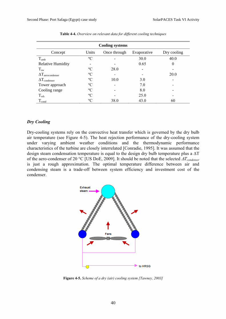
Second Phase: Port Safaga (Egypt) case study SolarPACES Task VI Activity
40
Table 4-4. Overview on relevant data for different cooling techniques
Cooling systems
Concept Units Once through Evaporative Dry cooling
Tamb ºC - 30.0 40.0
Relative Humidity - - 0.65 0
Tsw ºC 28.0 - -
ΔTaerocondenser ºC - - 20.0
ΔTcondenser ºC 10.0 3.0 -
Tower approach ºC - 7.0 -
Cooling range ºC - 8.0 -
Twb ºC - 25.0 -
Tcond ºC 38.0 43.0 60
Dry Cooling
Dry-cooling systems rely on the convective heat transfer which is governed by the dry bulb
air temperature (see Figure 4-5). The heat rejection performance of the dry-cooling system
under varying ambient weather conditions and the thermodynamic performance
characteristics of the turbine are closely interrelated [Conradie, 1995]. It was assumed that the
design steam condensation temperature is equal to the design dry bulb temperature plus a T
of the aero-condenser of 20 °C [US DoE, 2009]. It should be noted that the selected Tcondenser
is just a rough approximation. The optimal temperature difference between air and
condensing steam is a trade-off between system efficiency and investment cost of the
condenser.
Figure 4-5. Scheme of a dry (air) cooling system [Tawney, 2003]

Second Phase: Port Safaga (Egypt) case study SolarPACES Task VI Activity
41
Evaporative Cooling
The evaporative cooling condenses the steam inside tube bundles that are constantly over-
sprayed with water from the cooling tower basin [Tawney, 2003] (Figure 4-6 and Figure 4-7).
Figure 4-6. Bottom of an evaporative tower (wetcooling.com)
Figure 4-7. Scheme of an Evaporative Tower cooling system [Tawney, 2003]
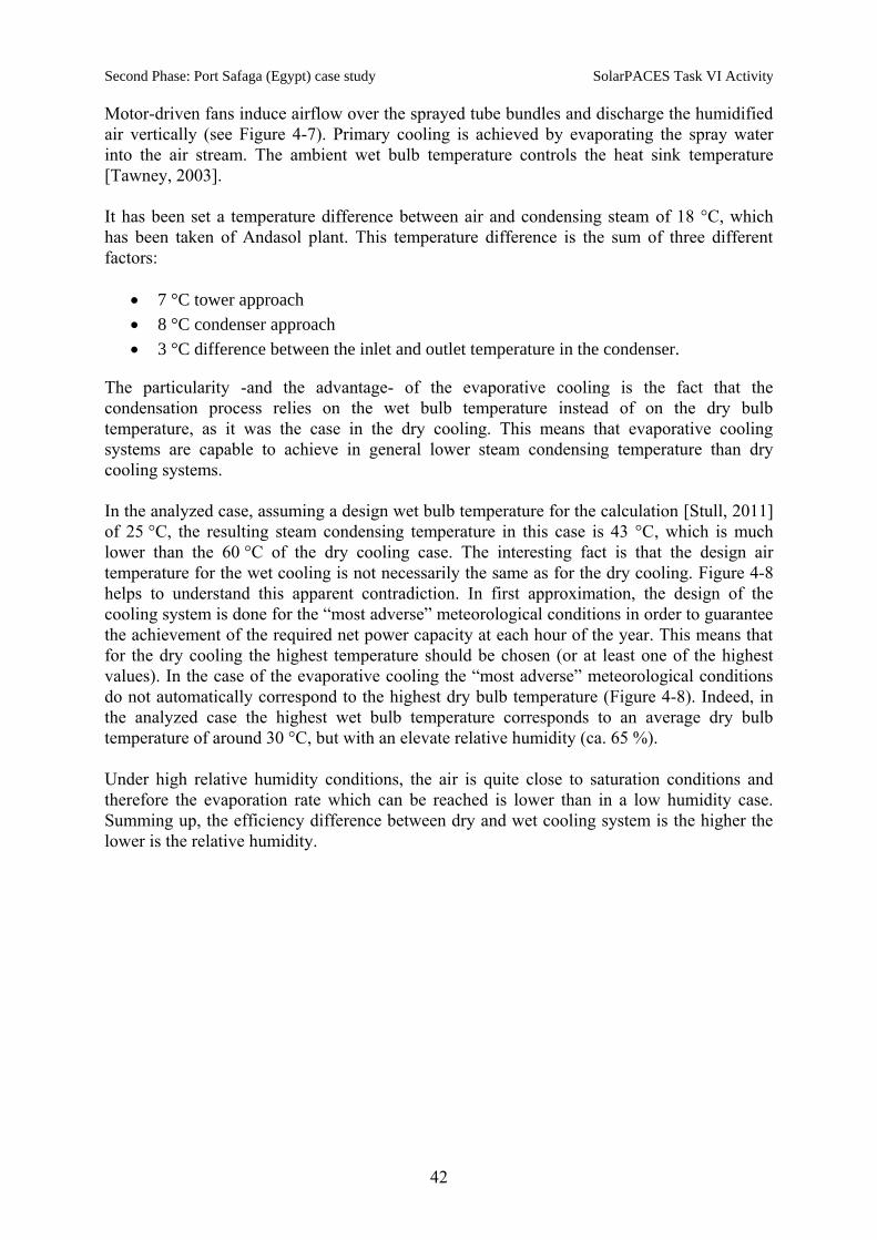
Second Phase: Port Safaga (Egypt) case study SolarPACES Task VI Activity
42
Motor-driven fans induce airflow over the sprayed tube bundles and discharge the humidified
air vertically (see Figure 4-7). Primary cooling is achieved by evaporating the spray water
into the air stream. The ambient wet bulb temperature controls the heat sink temperature
[Tawney, 2003].
It has been set a temperature difference between air and condensing steam of 18 °C, which
has been taken of Andasol plant. This temperature difference is the sum of three different
factors:
7 °C tower approach
8 °C condenser approach
3 °C difference between the inlet and outlet temperature in the condenser.
The particularity -and the advantage- of the evaporative cooling is the fact that the
condensation process relies on the wet bulb temperature instead of on the dry bulb
temperature, as it was the case in the dry cooling. This means that evaporative cooling
systems are capable to achieve in general lower steam condensing temperature than dry
cooling systems.
In the analyzed case, assuming a design wet bulb temperature for the calculation [Stull, 2011]
of 25 °C, the resulting steam condensing temperature in this case is 43 °C, which is much
lower than the 60 °C of the dry cooling case. The interesting fact is that the design air
temperature for the wet cooling is not necessarily the same as for the dry cooling. Figure 4-8
helps to understand this apparent contradiction. In first approximation, the design of the
cooling system is done for the “most adverse” meteorological conditions in order to guarantee
the achievement of the required net power capacity at each hour of the year. This means that
for the dry cooling the highest temperature should be chosen (or at least one of the highest
values). In the case of the evaporative cooling the “most adverse” meteorological conditions
do not automatically correspond to the highest dry bulb temperature (Figure 4-8). Indeed, in
the analyzed case the highest wet bulb temperature corresponds to an average dry bulb
temperature of around 30 °C, but with an elevate relative humidity (ca. 65 %).
Under high relative humidity conditions, the air is quite close to saturation conditions and
therefore the evaporation rate which can be reached is lower than in a low humidity case.
Summing up, the efficiency difference between dry and wet cooling system is the higher the
lower is the relative humidity.
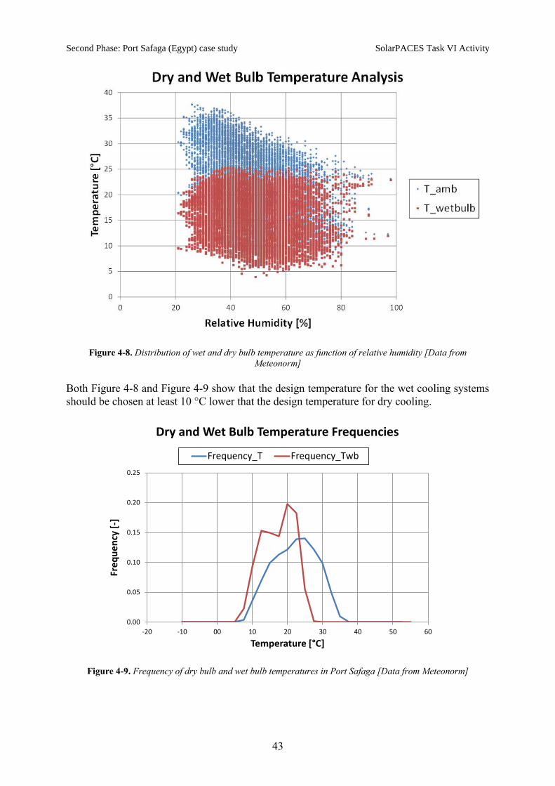
Second Phase: Port Safaga (Egypt) case study SolarPACES Task VI Activity
43
Figure 4-8. Distribution of wet and dry bulb temperature as function of relative humidity [Data from
Meteonorm]
Both Figure 4-8 and Figure 4-9 show that the design temperature for the wet cooling systems
should be chosen at least 10 °C lower that the design temperature for dry cooling.
Figure 4-9. Frequency of dry bulb and wet bulb temperatures in Port Safaga [Data from Meteonorm]
0.00
0.05
0.10
0.15
0.20
0.25
-20 -10 00 10 20 30 40 50 60
Fre
qu
en
cy [
-]
Temperature [°C]
Dry and Wet Bulb Temperature Frequencies
Frequency_T Frequency_Twb

Second Phase: Port Safaga (Egypt) case study SolarPACES Task VI Activity
44
In this phase the parasitics corresponding to the solar field, thermal storage, steam turbine, the
cooling systems and the desalination plant have been assessed in detail. In the following are
listed the assumptions which have been selected for the calculation of the each one.
Solar Field
The parasitics for the solar field can be calculated by the following equation:
·
·sf
sf HTF
parasitics
HTF pump
P mP
(6)
where
Pparasitics_sf is the electricity consumption for HTF pumping, in MWel,
Psf the pressure drop of the HTF in the solar field, in bar,
mHTF the HTF mass flow, in kg/s,
HTF is the HTF density, in kg/m³ and
pump is the HTF pump efficiency.
The pressure drop (ΔPsf) of the HTF in the solar field under design conditions is a function of
the size of the solar field, in m²:
12 2 53.59 10 · 1.28·10 · 10.2sf sf sfP A A (7)
The pump efficiency (ηpump) was assumed to be 80%. The density of the heat transfer fluid
(VP-1) was calculated for the average temperature in the solar field according to Solutia.
Finally, the reference mass flow was evaluated with a simplified approach:
·HTF
sf
HTF
sf p
Qm
T c
(8)
where
Tsf is the HTF temperature difference between inlet and outlet of the collector, in K,
and
cp_HTF is the HTF specific heat, in kJ/kg/K.
Thermal Energy Storage
The consumption of the molten salt pump was calculated according to Morin (2010) and
adjusted with a correction factor in order to take into account additional pressure drops in the
piping and in the heat exchanger:
0.003·TES
TESdesign
netparasitics
th
PP
Q (9)
where
Pparasitics_TES is the internal power consumption of the molten salt pump, in MW and
Qth_TES_design is the storage thermal charge flow at design conditions, in MWhth.

Second Phase: Port Safaga (Egypt) case study SolarPACES Task VI Activity
45
Steam Turbine
The internal power consumption of the power block consists of the parasitics of the two feed
water pumps, which have been calculated directly in the power cycle model by the following
equation:
·turb
wparasitics
pump
h mP
(10)
where
Pparasitics_turb is the internal power consumption of the steam turbine, in MW,
h is the feed water enthalpy jump provided by the pump, in kJ/kg,
mw is the feed water mass flow, in kg/s and
pump is the feed water pump efficiency.
Cooling Systems
In order to evaluate the power consumption of the cooling systems, specific values have been
obtained from Sokrates (2004) and using software of hydraulic calculus:
Table 4-5. Specific internal electricity consumption of the analyzed cooling systems
Specific parasitics of cooling systems
Once-through 0.0104 MWel/MW
Evapor. Cooling 0.0329 MWel/MW
Dry cooling 0.0431 MWel/MW
MED 0.0 MWel/MW
For the cooling water piping it is assumed that the plants are located at an altitude of 20 m
above the sea level and a distance from the shore of about 2.2 km.
Desalination
As it was mentioned before, for the desalination plants, a specific power consumption of
4.5 kWh/m³ for RO and 1.6 kWh/m³ for MED have been considered. The used specific power
consumptions take into account the desalination process as well as the pressure losses
occurring in the piping of the feed water and of the brine. It is assumed that the desalination
plants are located at an altitude of 20 m above the sea level and a distance from the shore of
about 2.2 km.
4.2.2. Calculation of the internal water consumption
As it was mentioned above, the MED case defines the net fresh water production for the RO
cases. In all the analyzed configurations, the net water production is slightly less than the
gross one, since a part of the water produced is consumed internally in the power plant for
cleaning the mirrors, for the power block water supply and other consumptions (drinking
water). Additionally, in the case of RO + evaporative cooling, an additional amount of water

Second Phase: Port Safaga (Egypt) case study SolarPACES Task VI Activity
46
in the desalination plant must be produced to be used in the cooling system. To determine the
specific water consumptions of the power block, the cooling tower and other consumptions
(drinking water), the distribution shown in Figure 4-10 has been taken, which refers to a case
of solar thermal power plant with evaporative cooling [Richter and Dersch, 2010].
Figure 4-10. Percentage of water consumed
in a solar thermal power plant with
evaporative cooling
In the reference case, this partition corresponds to total amount of 3,800 l/MWe,net. In the case
of mirror cleaning, a specific consumption of 27 l/(m2·y) has been set in all cases studied
[Richter and Dersch, 2010]. This value was adjusted by an empiric factor in order to adapt the
cleaning frequency to the analyzed site.
When once-through cooling is considered, the specific seawater consumed in the condenser is
calculated as follows:
· ·
· ·.
turb outout out
cw cw
S Sturb
p condenser p condensercw
gross gross gross
m xQ
c T c TmSpec SW
P P P
(11)
where
mcw is the cooling water mass flow, in kg/s,
Qturb_out is the heat flow at the turbine outlet, in MWhth,
cpcw is the specific heat of cooling water, in kJ/kg/K,
ms_turb_out is the steam mass flow at the turbine outlet, in kg/s,
is the steam latent heat of condensation, in kJ/kg and
xs_out is the steam moisture fraction at the turbine outlet.
The resulting specific water consumptions are summarized in the following table.
Table 4-6. Water consumption
Water consumption
Specific water
consumption
Units Once through
+ RO
Evap. cooling
+ RO
Dry cooling
+ RO
MED
Cooling l/MWhel_gross 144,874.7 2,969.5 0.0 0.0
Power block l/MWhel_gross 197.3
Mirror washing l/(m2·year) 27
Factor for mirror cleaning − 1.3
Mirror washing (adj.) l/(m2·year) 35.1
Various (drinking water) l/MWhel_gross 3.2
Power block
Mirror washing
Drinking water
Cooling tower

Second Phase: Port Safaga (Egypt) case study SolarPACES Task VI Activity
47
4.3. Economic analysis
The same procedure to calculate the LEC and the LWC as it was explained in the phase 1 has
been used for this phase of the project. In the following tables (Table 4-7 to Table 4-13), all
the input parameters that have been used for power and water cost calculation are shown.
They have been taken from the literature [NREL, 2010; Tawney et al., 2003] and personal
communication. As it can be seen in Table 4-12, it has been assumed and additional power
production of 15 % with natural gas.
Table 4-7. Summary of the cost assumptions
Assumptions
Concept Unit/Reference Once through
+ RO
Evap.
cooling + RO
Dry cooling
+ RO MED
Interest rate %/tot_inv/y 6.5
Insurance rate %/tot_inv/y 1.0
Plant life y 20
Total land
requirement Ha 200
Parasitic loads net yearly power
production 10%
Plant availability − 0.96
Table 4-8. Input data to calculate the direct capital costs
Direct capital costs
Concept Units Once through
+ RO
Evap. cooling
+ RO
Dry cooling
+ RO MED
Spec. inv. SF €/m2 200
Spec. inv. TES $/kWhth 40a
Spec. inv. Power Block €/kW 689.1b
Spec. inv. cooling €/kWel 40.22b 62.86b 239b 0
Spec. inv. DES €/(m³/d) 965.6c 965.6c 965.6c 984c
Auxiliary gas burner €/kWth 42d
HTF and hydraulic
circuit €/m2 72d
Land preparation and
infrastructure €/m2 27
d
Contingency €/m2 5.0%d
a: PC (personal communication) b: NREL, 2010; Tawney et al., 2003 c: GWI, 2010 d: NREL, 2010

Second Phase: Port Safaga (Egypt) case study SolarPACES Task VI Activity
48
Table 4-9. Input data to calculate the indirect project costs
Indirect project costs
Concept Reference Once through
+ RO
Evap.
cooling + RO
Dry cooling
+ RO MED
EPC and related
costs
Direct
Capital Costs 12.5%e
Permiting, licenses
and legal
Direct
Capital Costs 2.5%e
e: PC
Table 4-10. Input data to calculate the costs manpower
Manpower costs
Concept Unit Once
through+ RO
Evap. cooling
+ RO
Dry cooling
+ RO MED
Management and administration people 8
Plant operation employees people 15
Solar field maintenance people 20 (3/100,000)
Power block and TES system people 8
Total desalination plant
personnel people 15
Reference yearly average
salaries (USA) € 51,959
Labor cost factor (Egypt) − 0.25
Table 4-11. Input data to calculate the operation and maintenance costs
Operation and maintenance costs (O&M)
Concept Unit Once through
+ RO
Evap. cooling
+ RO
Dry cooling
+ RO MED
Site Land cost 0.30%f
Solar field Solar field
cost 0.30%f
HTF HTF cost 0.30%f
TES TES cost 0.30%f
Power block
fixed cost
Gross
turbine prod. 27,000 €/MWe
f
Power block
variable cost
Total gross
yearly power
prod.
2.0 €/MWhg
Recovery ratio
desalination plant − 45% 45% 45% 35%
Chemical
consumptions
Total
seawater
processing
1.62€/m3 1.62€/m3 1.62€/m3 0.024€/m3
f: PC (personal communication) g: NREL, 2010
n/a: not available
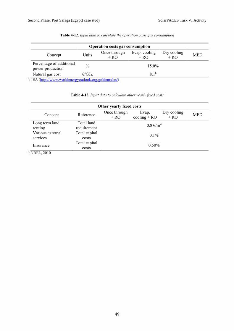
Second Phase: Port Safaga (Egypt) case study SolarPACES Task VI Activity
49
Table 4-12. Input data to calculate the operation costs gas consumption
Operation costs gas consumption
Concept Units Once through
+ RO
Evap. cooling
+ RO
Dry cooling
+ RO MED
Percentage of additional
power production % 15.0%
Natural gas cost €/GJth 8.1h h: IEA (http://www.worldenergyoutlook.org/goldenrules/)
Table 4-13. Input data to calculate other yearly fixed costs
Other yearly fixed costs
Concept Reference Once through
+ RO
Evap.
cooling + RO
Dry cooling
+ RO MED
Long term land
renting
Total land
requirement 0.8 €/m2i
Various external
services
Total capital
costs 0.1%i
Insurance Total capital
costs 0.50%i
i: NREL, 2010

Second Phase: Port Safaga (Egypt) case study SolarPACES Task VI Activity
50
4.4. Results
4.4.1. Thermodynamic analysis
In this final section main technical results are presented and commented (Table 4-14). It can
be seen that –according to the design assumptions- the gross power generation in the different
cases varies up to ca. 9 MW. This can be explained with the different internal power
consumption of the system components. The most relevant factors are the parasitics of the
desalination plant; the power consumption of the MED is in fact roughly 1/3 of the
consumption of the RO. Therefore in all RO cases a larges gross capacity is required in order
to achieve the 50 MW of net power production.
Table 4-14. Summary table with main power cycle parameters
Power cycle
Concept Units Once-trough +
RO
Evap. Cooling
+ RO
Dry Cooling
+ RO MED
Pgross MWel 65.8 68.3 69.4 60.2
Pnet MWel 50.0 50.0 50.0 50.0
ηturb_th − 39.4% 38.7% 36.0% 34.5%
ηturb_gross − 38.3% 37.5% 35.0% 33.5%
ηturb_net (CSP w/o TES) − 33.9% 32.3% 29.4% 29.4%
ηturb_sys (inc DES.) − 29.1% 27.5% 25.3% 27.8%
Qturb_in MW 172 182 198 180
Tcond ºC 38.0 43.0 60.0 70.0
Ppar_SF MWel 5.1 5.5 6.2 5.4
Ppar_TES MWel 0.9 1.0 1.1 1.0
Ppar_TURB MWel 0.9 0.9 1.0 0.9
Ppar_COOL MWel 0.7 2.2 2.9 0.0
Ppar_DES MWel 8.2 8.6 8.2 2.9
mturb_in kg/s 76.02 08.44 87.66 79.59
mturb_out kg/s 48.68 51.97 58.40 54.02
xout − 0.89 0.89 0.92 0.93
A second important factor is the condensation temperature in the different analyzed cooling
systems. In principle, the higher the design condensing temperature, the lower the efficiency
(thermal, gross and net) of the power block. In turn, the lower the thermal turbine efficiency,
the higher the heat requirements and the higher the number of required solar field collectors.
Finally, the larger the solar field, the larger are the parasitics of the solar field.
As expected, the most efficient cooling method is the once-through, followed by the
evaporative cooling. Dry cooling and MED deliver the lowest cooling efficiencies. The dry
cooling case presents the largest gross turbine capacity and requires the largest solar field
(198 loops vs. 172 loops in the once-through case). Also, the dry cooling shows the highest
internal power consumption for the cooling system (2.9 MW), which occurs due to the fans,
while in the case of the MED the cooling parasitics are zero, since cooling water pumping is
already taken into account in the desalination parasitics.

Second Phase: Port Safaga (Egypt) case study SolarPACES Task VI Activity
51
Finally, it is interesting to see that the system efficiency sys, which is defined as:
in
netsys
turb
P
Q (12)
is higher for the MED case (27.8 %) than for the wet cooling and dry cooling systems (27.5 %
and 25.3 %, respectively) although the thermal efficiency in the MED case is the lowest one.
This can be explained again with the relatively low internal power consumption of the MED
in comparison to the RO.
Finally, in the Table 4-15 the internal water consumption and the gross and net water
produced by the desalination plants are shown:
Table 4-15. Summary table with water consumptions
Desalination and water consumption
Concept Units Once-trough +
RO
Evap. Cooling
+ RO
Dry Cooling
+ RO MED
Gross water capacity
DES m3/d 43,640 46,066 43,659 43,630
Water consumption
cooling m3/d 0.0 2,416.0 0.0 0.0
Water consumption pb m3/d 154.7 160.5 163.1 141.6
Water consumption sf m3/d 60.4 64.2 69.8 63.5
Water consumption
various m3/d 5.2 5.3 5.4 4.7
Required water
production DES m3/d 43.420 43,420 43,420 43,420 Pb=power block; sf=solar field
4.4.2. Economic analysis
From the results obtained from the technical analysis, an annual analysis of the CSP and the
desalination systems has been carried out in order to obtain the annual costs of both, required
to calculate the LEC and the LWC (equations (2) and (3)).
The results obtained from the annual analysis are shown in Table 4-16 and Table 4-17. The
annual DNI has been taken from meteorological data of Port Safaga (DLR). The equivalent
yearly operation hours have been determined by the following correlation [Trieb et al., 2009]:
2(2.5717· 694)·( 0.0371· 0.4171· 0.0744)FLH DNI SM SM (13)
where SM is the solar multiple, which has been considered 1.9
The capacity factor is assessed straightaway from the ratio between FLH with respect the total
hours in a year (8,760 hours).

Second Phase: Port Safaga (Egypt) case study SolarPACES Task VI Activity
52
Table 4-16. Annual analysis of the CSP plant
Annual Analysis CSP
Concept Units Once-trough
+ RO
Evap.
Cooling + RO
Dry Cooling
+ RO MED
DNI kWh/(m²y) 2,486
FLH h/y 4,140
Capacity factor − 0.47
Parasitic cooling Mwel-h/y 2,740 9,019 11,928 0
Parasitic loads MWel-h/y 19,874 19,874 19,874 19,874
Pel_net_tot GWh/y 198.7 198.7 198.7 198.7
Pel_net_tot
(including 15% gas) GWh/y 228.6 228.6 228.6 228.6
Pel_gross_tot GWh/y 262.1 268.7 264.1 230.4
Pel_gross_tot
(including 15% gas) GWh/y 301.4 309 303.7 265
Table 4-17. Annual analysis of the desalination plant
Annual Analysis DES
Concept Units Once-trough
+ RO
Evap. Cooling
+ RO
Dry Cooling
+ RO MED
Water consumed
by the CSP plant Mio. m3/y 0.08 0.08 0.09 0.08
Water consumed
by the cooling tower Mio. m3/y n/a 0.9 n/a n/a
Total Water
Production Mio. m³/y 7.4 7.9 7.5 7.4
The results of the annual costs are summarized in
Table 4-18 to Table 4-20. Finally, the Table 4-21 gives the results of the power and water
costs for the configurations analyzed.
Table 4-18. Investment Cost results for the CSP and DES plants
Annual Analysis DES
Concept Units Once-trough
+ RO
Evap. Cooling
+ RO
Dry Cooling
+ RO MED
Solar Field Mio. € 126.9 135.4 146.5 132.1
Land preparation
and infrastructure Mio. € 43.2 43.2 43.2 43.2
HTF and hydraulic circuit Mio. € 45.7 48.7 52.7 47.6
TES Mio. € 44.6 47.6 51.5 46.4
Power Block Mio. € 45.5 47.6 48.0 41.5
Cooling Mio. € 2.7 4.3 16.6 0
Auxiliary gas burner Mio. € 7.2 7.1 8.3 7.5
DES Mio. € 43.4 53.1 43.4 43.9

Second Phase: Port Safaga (Egypt) case study SolarPACES Task VI Activity
53
Table 4-19. Annual costs of the CSP plant
Annual costs CSP
Concept Units Once-trough
+ RO
Evap. Cooling
+ RO
Dry Cooling
+ RO MED
Total capital cost Mio. € 331.3 350.4 385.2 334.2
Total project cost Mio. € 49.7 52.6 57.8 50.1
Yearly labour cost Mio. € 0.7 0.7 0.7 0.7
Yearly maintenance cost Mio. € 3.2 3.3 3.4 3.0
Natural gas yearly cost Mio. € 3.9 4.3 4.6 3.6
Other yearly cost Mio. € 3.6 3.7 3.9 3.6
Total O&M cost Mio. € 11.3 12.0 12.5 10.8
crf annuity factor % 10.08% 10.08% 10.08% 10.08%
Table 4-20. Annual costs of the desalination plant
Annual costs DES
Concept Units Once-trough
+ RO
Evap. Cooling
+ RO
Dry Cooling
+ RO MED
Total capital cost Mio. € 43.4 53.1 43.4 43.9
Total project cost Mio. € 6.5 8.0 6.5 6.6
Yearly labour cost Mio. € 0.2 0.2 0.2 0.2
Yearly maintenance cost Mio. € 0.5 0.7 0.6 0.8
Other yearly cost Mio. € 0.3 0.4 0.3 0.3
Total O&M cost Mio. € 1.0 1.2 1.0 1.3
crf annuity factor % 10.08% 10.08% 10.08% 10.08%
Table 4-21. Results of the power and water costs
Power and water costs
Concept Units Once-trough
+ RO
Evap. Cooling
+ RO
Dry Cooling
+ RO MED
LEC €cent/kWh 21.75 23.00 25.01 21.68
LWC €/m³ 0.83 1.00 0.83 0.87
Additionally, the variation of the power cost has been studied with respect the cost of the
solar field. For this purpose, the specific investment of the solar field has been varied from
150 to 250 €/m2. The results obtained are shown in Figure 4-11.

Second Phase: Port Safaga (Egypt) case study SolarPACES Task VI Activity
54
Figure 4-11. Variation of the LEC with the cost of the solar field
4.5. Additional Report – Yearly Simulation Draft
This additional part of the report gives an overview of the bachelor thesis of the student
Christian Schwager, a work carried out in parallel and in collaboration to the work of
Massimo Moser and Patricia Palenzuela within the Task VI of the SolarPACES activities
[Schwager, 2012]. His work represents a first step of the required further analyses in order to
characterize more in detail the optimal design and layout of the CSP+DES plant.
The boundary conditions based on location, meteorology and demands are:
- 30 m above sea level
- 2.2 km distance to the shore
- 2,869 kWh/m²a DNI
- 26.3 °C average ambient temperature during CSP operation
- 24.8 °C average sea water temperature
- Parabolic though CSP-plant
- 6.5 h molten salts storage
- The same amount of annual fresh water production for all configurations
19
20
21
22
23
24
25
26
27
28
100 150 200 250 300
Spec Inv SF (€/m2)
LEC
(c€
/kW
h)
MED
Once Through+RO
Evap.Cooling +RO
Dry Cooling+RO

Second Phase: Port Safaga (Egypt) case study SolarPACES Task VI Activity
55
Figure 4-12. Land use estimation and solar field size
In this study there four different desalination technologies were analyzed. They are:
1. Dry cooled (ACC) CSP plant with reverse osmosis (RO)
2. Once-Through (OTC) cooled CSP plant with reverse osmosis (RO)
3. CSP with multiple effect distillation (MED)
4. CSP with membrane distillation (MD)
This study is mainly structured in two parts. In the first part the design performances are
analyzed, while in the second part of the work operation strategies and yearly simulations of
the plant are taken into account. The analysis is completed by an optimization process by
means of LEC calculation for different plant configurations. The optimized variables are solar
field size and capacity of the thermal storage.
4.5.1. Steady-State Operating Performance
First, the different combinations of power block and desalination are modeled and simulated
under design conditions. Main design parameter assumptions can be found in the appendix of
[Schwager 2012]. The design results (net power production and desalination capacity) are
presented in Figure 4-13 and Figure 4-14.
Figure 20 shows the results for the electricity production under design conditions (180 MWth
at turbine inlet) for the 4 analyzed configurations. The water production is defined through the
MED case and is kept constant in the 2 RO cases (1,534.28 m³/h).
Due to the high turbine outlet temperature in configuration 1 (CSP-ACC+RO), caused by the
low heat transfer coefficient of air, the efficiency is significantly lower compared to the sea
water cooled system. Therefore configuration 1 is not included in the annual yield
simulations. Configuration 4 (PB-OTC+MD) is the less efficient configuration, due to the
high heat losses in the brine exhaust and exergy losses inside the MD modules.
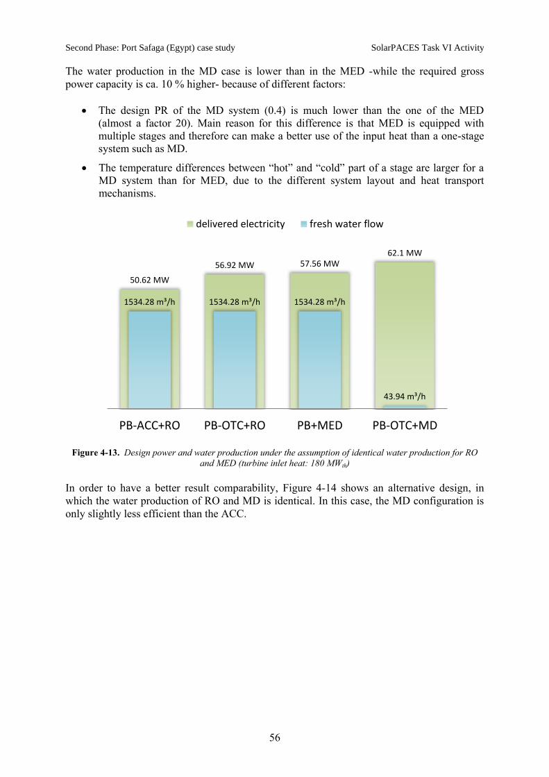
Second Phase: Port Safaga (Egypt) case study SolarPACES Task VI Activity
56
The water production in the MD case is lower than in the MED -while the required gross
power capacity is ca. 10 % higher- because of different factors:
The design PR of the MD system (0.4) is much lower than the one of the MED
(almost a factor 20). Main reason for this difference is that MED is equipped with
multiple stages and therefore can make a better use of the input heat than a one-stage
system such as MD.
The temperature differences between “hot” and “cold” part of a stage are larger for a
MD system than for MED, due to the different system layout and heat transport
mechanisms.
Figure 4-13. Design power and water production under the assumption of identical water production for RO
and MED (turbine inlet heat: 180 MWth)
In order to have a better result comparability, Figure 4-14 shows an alternative design, in
which the water production of RO and MD is identical. In this case, the MD configuration is
only slightly less efficient than the ACC.
50.62 MW
56.92 MW 57.56 MW62.1 MW
1534.28 m³/h 1534.28 m³/h 1534.28 m³/h
43.94 m³/h
. m³/h
500. m³/h
1000. m³/h
1500. m³/h
2000. m³/h
2500. m³/h
. MW
10. MW
20. MW
30. MW
40. MW
50. MW
60. MW
70. MW
PB-ACC+RO PB-OTC+RO PB+MED PB-OTC+MD
delivered electricity fresh water flow

Second Phase: Port Safaga (Egypt) case study SolarPACES Task VI Activity
57
Figure 4-14. Design power and water production under the assumption of identical water production for RO
and MD (turbine inlet heat: 180 MWth)
4.5.2. Annual Simulation and Economical Calculation
Based on the previous analysis, annual simulations and economic analysis are carried out. In
this way it is possible to simulate the behavior of the plant under part load conditions, to
estimate the annual electricity and water production yield and to compare different
configurations among each other in terms of LEC and LWC.
The required meteorological input values are taken from Meteonorm. In this simulation the
startup losses of the solar field, the thermal storage and the power block are considered.
Besides the operation strategies are adapted to each desalination technology.
The selected configurations for the annual yield simulation are:
- 2a: CSP-OTC+RO - 24h full load operation for desalination, PB solar-only
- 2b: CSP-OTC+RO - solar-only
- 3a: CSP+MED - 24h full load operation
- 3b: CSP+MED - 24h operation, 85% part load during fossil backup
- 4: CSP-OTC+MD - solar-only
Figure 4-15 explains the structure of the simulation model. First, each hour of the year the
input parameters (mainly DNI, ambient temperature and wind velocity) are red. The solar
field model calculates the collected heat. Different loss mechanisms such as optical,
geometrical and thermal losses are taken into account. If at a certain time (typically in the
early morning) the temperature of the working fluid in the solar field is below the design
value, additional heat losses (so-called “start-up” losses) have to be considered, till the
working fluid reaches operation conditions. In the further steps of the calculation, the heat
collected in the solar field is compared with the heat requirements of the turbine. Accordingly,
the thermal energy storage is charged or discharged or the fossil back-up is operated. If the
59.28 MW
65.58 MW
57.56 MW62.1 MW
34.94 m³/h 34.94 m³/h
1534.28 m³/h
43.94 m³/h
. m³/h
500. m³/h
1000. m³/h
1500. m³/h
2000. m³/h
2500. m³/h
. MW
10. MW
20. MW
30. MW
40. MW
50. MW
60. MW
70. MW
PB-ACC+RO PB-OTC+RO PB+MED PB-OTC+MD
delivered electricity fresh water flow

Second Phase: Port Safaga (Egypt) case study SolarPACES Task VI Activity
58
heat collected by the solar heat is larger than the turbine requirement and the thermal storage
is completely charged, heat from the solar field has to be dumped, i.e. the mirrors have to be
defocussed. Finally, gross and net power generation and water production are calculated.
Figure 4-15. Overview of calculation scheme for annual yield analysis with hourly time step
The size of all components is assessed during the design process. As the net power production
and the storage capacity are assumed to be fixed, the optimal field size is defined by the
lowest LEC. In configuration 3 the LEC is minimal for a solar field with an aperture equal to
zero. Therefore the gas-driven backup needs to be turned off for the design simulations. After
designing configuration 3a/b, the resulting net water production is assumed for configuration
2a/b, as well, while configuration 4 is designed independently.
Figure 4-16 presents the energy flows for the once-through cooled CSP plant with reverse
osmosis and the CSP+MED.
optical losses
DNI ofhour
deduction ofstart-up energy
deduction ofstart-up energy
thermal losses
determining nominal required heat
determiningrequired heat
during discharge
additional power is stored
max. load, remainingpower is overload
dumping
deduction ofstart-up energy
Tfield < Tfield,n
Qcont,stor < Qcont,stor,n
ΔtPB,offline > 4h
>
limited backupfrom storage
determining grosspower generation
determiningfresh water
flow
deduction ofonline parasitics
deduction ofoffline parasitics
Pel,netPel,required

Second Phase: Port Safaga (Egypt) case study SolarPACES Task VI Activity
59
Figure 4-16. Energy flow diagram for the CSP-OTC+RO (left) and CSP+MED (right) configurations
Table 4-22 shows selected results of the annual yield simulations. Configuration 4 presents a
negative net water production, because the required fresh water for mirror cleaning and steam
cycle make-up is higher than the gross water production. For this reason configuration 4 is
excluded from further economical calculations.
Table 4-22. Main results from annual yield simulation for the analysed configurations
Power and water costs
Concept Units
CSP-OTC+RO
24h 100%
2a
CSP-OTC+RO
solar-only
2b
CSP+MED
24h 100%
3a
CSP+MED
24h >85%
3b
CSP-OTC+MD
solar-only
4
Aapertur m2 546,090 591,870 526,470 526,470 467,610
Pgross,n kW 68,559 76,640 61,754 61,754 59,361
Wel,net MWh/y 212,217 210,194 445,201 390,387 210,265
qwater,net m3/y 12,785,664 11,725,480 12,785,664 11,725,480 -27,883
mCO2 T/y 27,492 2,077 175,931 144,202 1,957
Based on the production amounts shown in Table 4-22 and cost assumptions [Schwager 2012,
appendix], LEC and LWC are calculated for each configuration (Figure 4-17). The lowest
LEC can be achieved with configuration 3a, but it also affects the highest CO2 emissions.
Also the fossil energy is used inefficiently compared to an optimized combined cycle power
plant.
However, it should be stressed that these LEC and LWC values were calculated for different
amounts of net generated power. Indeed, in both MED cases the net power production is
almost 2 times the power production in cases 2a and 2b.
optical losses
storage
electricity
parasitics
fresh water
waste heatthermal losses
optical losses
storage
electricity
parasitics
fresh water
waste heat
thermal losses
DN
I o
n a
pe
rtu
re

Second Phase: Port Safaga (Egypt) case study SolarPACES Task VI Activity
60
Figure 4-17. LEC and LWC for the analysed configurations
The results sensitivity of the LEC on CO2 is shown in Figure 4-18. The results make clear that
only very high CO2 costs have an effect on the cost advantage of configuration 3a/b.
Figure 4-18. LEC sensitivity on CO2 costs
Finally, the LEC sensitivity on the capacity of the thermal storage is shown in Figure 4-19.
Here it can be observed that a slight reduction of the LEC -and a more pronounced of the
LWC- can be achieved by increasing the thermal storage capacity.
0.172 0.177
0.106 0.114 0.135
0.377
0.679
0.4600.502
2a 2b 3a 3b
CSP-OTC+RO24h 100%
CSP-OTC+ROsolar-only
CSP+MED24h 100%
CSP+MED24h >85%
CSP-OTCsolar-only
LEC [€/kWh]
LWC [€/m³]
0.1
0.11
0.12
0.13
0.14
0.15
0.16
0.17
0.18
0.19
0.2
0 50 100 150 200
LEC
[€
/kW
h]
CO2-costs [€/T]
LEC CSP-OTC+RO 24h 100%
LEC CSP-OTC+RO solar-only
LEC CSP+MED 24h 100%
LEC CSP+MED 24h >85%
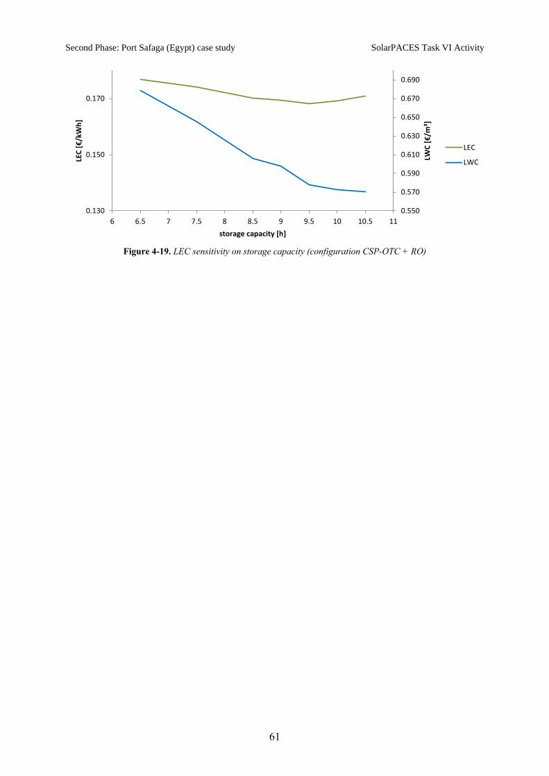
Second Phase: Port Safaga (Egypt) case study SolarPACES Task VI Activity
61
Figure 4-19. LEC sensitivity on storage capacity (configuration CSP-OTC + RO)
0.550
0.570
0.590
0.610
0.630
0.650
0.670
0.690
0.130
0.150
0.170
6 6.5 7 7.5 8 8.5 9 9.5 10 10.5 11
LWC
[€
/m³]
LEC
[€
/kW
h]
storage capacity [h]
LEC
LWC

5. Conclusions: potential of CSP+D concept at Egypt and MENA
countries
It is clear that CSP technology is a very promising option to achieve all these goals and, when
combined power and water production is considered, the following two concepts exist:
a) CSP Plants for co-generation with coupled seawater desalination using thermal
processes (MED/MSF). Their electricity can be used for additional Reverse Osmosis
desalination (RO), for domestic electricity consumption or for export. Main
inconvenience of this option is the necessity to be at coastal regions, which are normally
strongly used by other human activities. In addition, direct normal solar irradiation
values are normally lower at coastal regions, limiting this type of plant to regions with
appropriate site conditions and available land area.
b) CSP Plants used exclusively for power generation can be anywhere on the grid. Their
electricity can be transmitted to the place where RO-desalination plant is located. This
type of plants can be placed where good irradiation coincides with good infrastructure
conditions.
Besides initially the second option seems to be the most adequate, with even slightly higher
current overall efficiencies when combined water and power production is considered, there
are still strong reasons to also support the full development of the first option. To this end, a
thermodynamic analysis of several configurations of CSP+D plants has been carried out
within this work.
The systems have been modelled for the ambient conditions of arid regions which impose dry
cooling in the power plant. In all cases, 50 MWe and 35,018 m3/day have been considered as
net power and net water production respectively, and 58ºC (0.18 bar abs) as the exhaust steam
outlet turbine conditions. The study has been carried out considering the location of Port
Safaga (Red Sea, Egypt), with an estimated yearly DNI of 2,496 kWh/m2. Considered
distance from the sea is between 2 and 5 km. This last figure is the maximum distance to the
sea to consider suitable for the facility.
The results have shown that, at 0.18 bars in the turbine outlet conditions, the configuration
that involves LT-MED is thermodynamically more efficient than the coupling of the CSP
plant with a RO desalination plant and needs a smaller solar field for the same production of
electricity. Moreover, this configuration has the advantage of not requiring any cooling.
A novel configuration of MED plant with thermo-compression, named LT-MED-TVC, has
been considered within this study. This configuration requires a larger solar field than the
combination of CSP+RO when the motive steam comes from the high pressure turbine.
However, the energy losses to the ambient are lower for this configuration, since the plant
cooling needs decrease in comparison with the CSP+RO case. Simulations have been carried
out taking into account steam extractions from the low pressure turbine at different pressure
conditions to make this technology more efficient thermodynamically.
The study shows that, for a value of 1.17 bars, the results obtained in the integration of the
LT-MED-TVC desalination unit into the CSP plant are very similar to those obtained with
CSP+RO. Therefore, in this case, the integration of a MED plant with thermo-compression

63
can also be a valid option for a CSP+D configuration in arid regions, especially considering
the lower cooling requirements of this case compared to the CSP+RO.
When costs are analyzed, comparing the two more efficient configurations (PT-CSP/RO and
PT-CSP/LT-MED), considering 58ºC/0.18 bar of exhaust turbine steam conditions and
5.46 kWh/m3 of Reverse Osmosis power requirements and 2.11 kWh/m
3 in the case of MED,
the results of final power + water costs, are very similar.
When all Egyptian coasts are analyzed, in the Mediterranean strip and considering radiation
and orographic constrains, 25 percent of the coast (900 km) can be considered suitable for
combined solar power and desalination facilities. In the case of the Red Sea (1,550 km), the
estimated percentage is about 40 percent. If 50 MW solar power plants and 40000 m3/day
desalination facilities are considered at 20 km distance intervals (reasonable distance to
provide power and water to nearby locations), the estimated number of suitable CSP+D units
at the Egyptian Mediterranean and Red Sea coast would be 11 and 31, respectively. This
would mean about 2.1 GW of installed power and 1.7 Mio. m3/d of installed desalination
capacity.
If the same percentages and estimations are considered to the rest of the MENA coasts
(assumption which, obviously, implies very high uncertainties), with about 6000 km of
additional coastline in the Red Sea and Persian Gulf and about 3700 km in the Mediterranean,
we arrive to the figures of 10.4 GW of power and 8.3 Mio. m3/day of desalination capacity.
However, this is a very simplistic approach which cannot be done in the case of locations
such as the Persian Gulf (with a huge demand for desalinated water) and countries such as
Saudi Arabia (with a significant number of thermal desalination facilities in the mainland
using brackish water as feedstock).

64
6. References
Along the present document the following references have been either cited or used.
[1] Blanco-Marigorta A.M., Sánchez-Enriquez, M.V., Peña-Quintana, J.A., Exergetic
comparison of two different cooling technologies for the power cycle of a thermal
power plant, Energy, Vol. 36, Issue 4, 2011, Pages 1966-1972.
[2] Conradie, A. E., Kröger, D. G., Performance Evaluation of Dry-Cooling Systems for
Power Plant Applications, Journal of Applied Thermal Engineering, Vol. 16, No. 3,
1995, Pages 219-232.
De Miguel A., Bilbao J., Test reference year generation from meteorological and
simulated solar radiation data, Solar Energy, Vol. 78, 2005, Pages 695-703.
[3] El-Nashar, A. M., Cogeneration for power and desalination - state of the art review,
Desalination Vol. 134, Issues 1-3, 2001, Pages 7-28.
[4] Forristall, R. Heat Transfer Analysis and Modeling of a Parabolic Trough Solar
Receiver Implemented in Engineering Equation Solver, 2003, Golden (USA, CO).
[5] Fritzmann C., Loewenberg J., Wintgens T., and Melin T.; “State-of-The-Art of reverse
osmosis desalination”, Desalination Vol. 216 (1-3), 2007, Pages 1-7.
[6] Geyer, M. et al., Dispatchable solar electricity for summerly peak loads from the solar
thermal projects Andasol-1 & Andasol-2. In: Proceedings of the 13th SolarPACES
Symposium, 2006, Sevilla, Spain.
[7] Global Water Intelligence, 2010.
[8] Google Earth, http://www.google.de/intl/de/earth/index.html, Accessed 26/07/2011.
[9] Hamed, O.A., Al-Washmi H.A., Al-Otaibi H.A., Thermoeconomic analysis of a
power/water cogeneration plant, Energy, Volume 31, Issue 14, November 2006,
Pages 2699-2709.
[10] Hirsch, T., Schenk, H., Dynamics of oil-based Parabolic Trough Plants - a Detailed
Transient Simulation Model, SolarPACES 2010.
[11] Holydaycheck website: http://www.holidaycheck.com/climate-wetter_Hurghada-
ebene_oid-id_2310.html, (Accessed June 2012)
[12] IEA Report, Golden Rules for a Golden Age of Gas – World Energy Outlook, Special
Report on Unconventional Gas, www.worldenergyoutlook.org
[13] Insel website, http://www.insel.eu, (Accessed July 2012)
[14] Lefevre M., Wald L., Diabate L., Using reduced data sets ISCCP-B2 from the
Meteosat satellites to assess surface solar irradiance. Solar Energy, Vol. 81, 2007,
Pages 240-253.
[15] McArthur, L. J. B., Baseline Surface Radiation Network (BSRN). Operations manual
V1.0. Serie: World Climate Research Programme. Secretariat of the World
Meteorological Organization, 1998, Geneva (Switzerland).
[16] Meyer R., Hoyer C., Schillings C., Trieb F., Diedrich E., Schroedter M., SOLEMI: A
new satellite-based service for high-resolution and precision solar radiation data for
Europe, Africa and Asia. DLR (Germany) 2004.

65
[17] Montes, M.J., Abanades, A., Martinez-Val, J.M.,Valdes, M., Solar multiple
optimization for a solar-only thermal power plant, using oil as heat transfer fluid in
the parabolic trough collectors, Journal of Solar Energy 83, 2009, Pages 2165-2176.
[18] Morin, G., Doctoral Thesis: Techno-Economical Design Optimization of Solar
Thermal Power Plants, 2010, Fraunhofer ISE.
[19] Moser M. et al., Combined water and electricity production on industrial scale in the
MENA countries with concentrating solar power. In: EuroMed 2010 Desalination for
Clean Water and Energy. Cooperation among Mediterranean Countries, October 3-7,
2010, Tel Aviv, Israel.
[20] NREL, 2010. https://sam.nrel.gov/cost [online]
[21] PC, Personal Communication.
[22] Pereira E. B., Martins F., Abreu S. L., Beyer H. G., Colle S., Perez R., Cross
validation of satellite radiation transfer models during SWERA project in Brazil.
Proceeding of the ISES Solar World Congress 2003, Göteborg (Sweden).
[23] Pérez R., Seals R., Zelenka A., Comparing satellite remote sensing and ground
network measurements for the production of site time specific irradiance data. Solar
Energy, Vol. 60, 1997, Pages 89-96.
[24] Pinker R. T., Ewing J. A.,. Modeling surface solar radiation: model formulation and
validation. Journal of Climate and Applied Meteorology, Vol. 24, 1985, Pages 389-
401.
[25] Pissimanis D., Karras G., Notaridou V., Gavra K., The generation of a "typical
meteorological year" for the city of Athens. Solar Energy, Vol. 40, 1988, Pages 405-
411.
[26] Polo J., Zarzalejo L.F., Ramirez L., Solar radiation derived from satellite images, in:
Modeling Solar Radiation at the Earth Surface. Edt: Viorel Badescu. Springer-Verlag,
2008, pp. 449-461.
[27] Polo J., Optimización de modelos de estimación de la radiación solar a partir de
imágenes de satélite. PhD presented at Complutense University of Madrid (Spain)
2009.
[28] Polo J., Zarzalejo L.F., Martin L., Navarro A.A., Marchante R., 2009a. Estimation of
daily Linke turbidity factor by using global irradiance measurements at solar noon.
Solar Energy, Vol. 83, 2009, Pages 1177-1185.
[29] Polo J., Zarzalejo L.F., Ramirez L., Espinar B., Iterative filtering of ground data for
qualifying statistical models for solar irradiance estimation from satellite data. Solar
Energy, Vol. 80, 2006, Pages 240-247.
[30] Ramírez L., Zarzalejo L.F., Polo J., Espinar B., Modelización de la radiación solar a
escala regional: Tratamiento de imágenes de satélite para cálculo de la radiación
solar global en España. 2º Congreso Internacional Ambiental del Caribe, 2004,
Cartagena de Indias (Colombia).
[31] Remund J., Domeisen D., Aerosol optical depth and Linke turbidity climatology.
Description for final report of IEA SHC Task 36, 2010.
[32] Richter, C., Dersch, J., Wasserverbrauch und Wassereinsparung bei solarthermischen
Kraftwerken, 2010, presentation at the DLR-Sonnenkolloquium.

66
[33] Richter C., Dersch J., Methods for reducing cooling water consumption in solar
thermal power plants, Proc. of the 16th SolarPaces Symposium. In: The CSP
Conference: Electricity, Fuels and Clean Water from Concentrated Solar Energy,
September, 15-18, 2009, Berlin, Germany.
[34] Rigollier C., Albuisson M., Delamare C., et al., 2000a. Explotaition of distributed
solar radiation databases through a smart network: the project SoDa. Proceedings of
2000 EuroSun Congress, Copenhagen (Denmark).
[35] Rigollier C., Bauer, O. y Wald, L., 2000b. On the clear sky model of the ESRA --
European Solar Radiation Atlas - with respect to the heliosat method. Solar Energy,
Vol. 68, 2000, Pages 33-48.
[36] Rigollier, C., Lefèvre, M. y Wald, L., The method Heliosat-2 for deriving shortwave
solar radiation from satellite images, Solar Energy, Vol. 77, 2004, Pages 159-169.
[37] Schwager, C., Bachelor Thesis: Technischer und wirtschaftlicher Vergleich
verschiedener Optionen zur Kopplung solarthermischer Stromerzeugung mit
Meerwasserentsalzung, Aachen University, 2012
[38] SIDEM website, http://www.sidem-desalination.com/en/process/Cogeneration/,
Accessed June 2011
[39] Short, W. et al. A manual for the economic evaluation of energy efficiency and
renewable energy technologies. NREL/TP-462-5173, 1995, Golden, CO, USA.
[40] Strauß, K., Kraftwerkstechnik zur Nutzung fossiler, nuklearer und regenerativer
Energiequellen, 2006, Dortmund.
[41] Stull, R., Wet-Bulb Temperature from Relative Humidity and Air Temperature,
American Meteorological Society, November 2011, Vancouver, Canada.
[42] Tawney, R., Khan, Z., Zachary, J., Economic and Performance Evaluation of Heat
Sink Options in Combined Cycle Applications, 2003, Atlanta (USA, GE).
[43] Therminol website, http://www.therminol.com/pages/products/vp-1.asp, (Accessed
March 2011)
[44] Toshiba website, http://www3.toshiba.co.jp/power/english/thermal/products/turbines/
ind3.htm, Accessed June 2011.
[45] Trieb, F., Concentrating solar power for seawater desalination, Aqua-CSP Study
report, German Aerospace Center, 2007, Sttutgart.
[46] Trieb, F., Kronshage, S., Quaschning, V., Dersch, J., Lerchenmüller, H., Morin, G.,
Häberle, A., Report: SOKRATES-Projekt Solarthermische Kraftwerkstechnologie für
den Schutz des Erdklimas, 2004, DLR, ISE, PSE.
[47] Trieb, F., Schillings, C., Viebahn, P., Paul, C., Altowaie, H., Sufian, T. et al., AQUA-
CSP: Concentrating Solar Power for Seawater Desalination. German Aerospace
Center (DLR), Study for the German Ministry of Environment, Nature Conservation
and Nuclear Safety, 2007, Stuttgart (Germany), www.dlr.de/tt/aqua-csp
[48] Trieb et al., Global Potential of Concentrating Solar Power. In Proc. SolarPACES
Conference 2009, Berlin (Germany).
[49] U.S. Department of Energy. Concentrating Solar Power Commercial Application
Study: Reducing Water Consumption of Concentrating Solar Power Electricity
Generation, 2009.

67
[50] Wetcooling website, http://www.wetcooling.com/, (Accessed July 2012)
[51] Worldenergyoutlook website, http://www.worldenergyoutlook.org/goldenrules/
[52] Yang L., Lam J. C., Liu J., Analysis of typical meteorological years in different
climates of China. Energy Conversion and Management, Vol. 48, 2007, Pages 654-
668.
[53] Zarzalejo L.F., Tellez F., Palomo E., Heras M.R., Creation of Typical Meteorological
Years (TMY) for Southern Spanish cities. Proceedings of the International Symposium
Passive Cooling of Buildings, 1995, Athens (Greece).
[54] Zarzalejo, L.F., Estimación de la irradiancia global horaria a partir de imágenes de
satélite. Desarrollo de modelos empíricos. PhD presented at Complutense University
of Madrid, 2005, Madrid (Spain).
[55] Zarzalejo L.F., Polo J., Martín L., Ramírez L., Espinar B., A new statistical approach
for deriving global solar radiation from satellite images. Solar Energy, Vol. 83, 2009,
Pages 480-484.
[56] Zelenka A., Perez R., Seals R., Renne D., Effective accuracy of satellite-derived
hourly irradiances. Theoretical and Applied Climatology, Vol. 62, 1999, Pages 199-
207.