assessment and design of multilateration telecommunication ... · joão vaz pato teixeira pinto...
TRANSCRIPT
Assessment and Design of Multilateration
Telecommunication Systems installed in NAV Portugal, EPE
João Vaz Pato Teixeira Pinto
Dissertation submitted for obtaining the degree of
Master in Electrical and Computer Engineering
Jury
Supervisor: Prof. Luís M. Correia
Co-Supervisor Eng. André Maia
President: Prof. José Bioucas Dias
Members: Prof. José Sanguino
Sep. 2011

ii

iii
To the Ones I love

iv

v
Acknowledgements
Acknowledgements
My first acknowledgement is to Prof. Luís Correia, the supervisor not only of the thesis but also of the
personal development during the past 8 months of work. From whom I acquired an exceptional
working method and support during this thesis development. I am also thankful for the hours spent
answering my questions, which are certainly worth a lot of money.
To the engineers from NAV Portugal, namely Eng. Carlos Alves, Eng. Luís Pissarro and Eng. André
Maia, whose contribution for the work is indisputable. Unfortunately stories are told that people from
external companies do not support you enough, but this was certainly not the case. I am thankful for
the numerous exchanged emails to clarify my doubts, the regular meetings to give feedback from the
work and the help developing the final document.
To the “Basement” colleagues, Diogo, Pedro, Ricardo, Tiago. Mainly due to the intellectual
discussions that stimulate the interest in each other thesis. Among ourselves we tried to use each
others as the first source to solve problems, at any hour or day. For them I wish the best success in
their working careers.
To all my friends, because life is not only just about work. Time spent partying with you is certainly the
best way to forget about the troubles in my life. To, Rita, Catarina, Inês, Margarida, Joana, Rui, Zé,
Jaime, João, José, Tiago, Miguel, Fernando, Diogo, Madalena, Jorge, Teresa, Cristina, for all the
support.
Last but not the least, I am thankful to my parents, grandparents, brothers and Filipa who no matter
what are always present in the good and the bad times. I am sorry for the lack of available time in the
last few months but I will certainly make it up.

vi

vii
Abstract
Abstract
Air space surveillance systems are continuously in progress to increase the space capacity and
safety. Multilateration is a proven technology to accurately identify aircraft. A latency model is
developed to study the influence of delay in multilateration system, using different communication
links. A coverage simulator is also developed as a tool for the study and design of new systems to be
implemented. Finally, additional requirements of this system are analysed for a better understanding
of it. In the latency model, it is shown that the influence of the delays is not important, and any kind of
link can be used to provide communication from the different sensors to the central processor. The
capacity of the links depends on the layers used for the communications, but for 250 airplanes the
required capacity is around 276 kbps. Finally, a minimum number of 4 sensors are enough to run the
location algorithm, but it does not meet the requirements for the tracking probability, a number in the
range {5, …, 10} being necessary to do so.
Keywords
Surveillance, Multilateration, Requirements, Delay, Coverage.
viii
Resumo
Resumo
Os sistemas de vigilância aérea estão continuamente em desenvolvimento com o objectivo de
melhorar quer a capacidade de gestão do espaço aéreo quer a segurança da operação.
Recentemente, apesar de conceptualmente ser já antiga, a Multilateração foi introduzida em sistemas
de vigilância para a navegação aérea, considerando as suas potencialidades e os baixos custos
associados. Um modelo de atraso é desenvolvido para estudar o efeito dos atrasos nos requisitos do
sistema e a influência dos diferentes tipos de canais de comunicação. Um simulador de cobertura foi
desenvolvido como ferramenta auxiliar para estudo e desenho de novos sistemas de multilateração
que se pretendam futuramente instalar. Finalmente, mais requisitos deste recente sistema são
analisados para melhor compreensão do funcionamento do seu próprio funcionamento. A influência
dos atrasos no sistema não é significativa e pode ser utilizado qualquer tipo de meio de transmissão.
A capacidade necessária em cada canal depende dos cabeçalhos usados, sendo que para 250
aviões será próxima de 276 kbps. Finalmente, o número mínimo de 4 sensores para executar o
algoritmo de localização, contudo não é suficiente para responder aos requisitos seguimento, sendo
necessário um número na gama de {5, …, 10} para os respeitar.
Palavras-chave
Vigilância, Multilateração, Requisitos, Atraso, Cobertura.

ix
Table of Contents
Table of Contents
Acknowledgements ................................................................................. v
Abstract ................................................................................................. vii
Resumo ................................................................................................ viii
Table of Contents ................................................................................... ix
List of Figures ....................................................................................... xii
List of Tables ........................................................................................ xiv
List of Acronyms ................................................................................... xv
List of Symbols ..................................................................................... xvii
List of Software ..................................................................................... xx
1 Introduction .................................................................................. 1
1.1 Overview.................................................................................................. 2
1.2 Motivation and Contents .......................................................................... 6
2 Basic Concepts ............................................................................ 7
2.1 Air Space Surveillance ............................................................................ 8
2.2 Multilateration ........................................................................................ 11
2.2.1 System Architecture ............................................................................................ 11
2.2.2 Time Difference of Arrival .................................................................................... 14
2.3 Telecommunications Systems Supporting Multilateration ..................... 15
2.3.1 Introduction .......................................................................................................... 15
2.3.2 Optical Fibre ........................................................................................................ 15
2.3.3 Microwave links ................................................................................................... 18
2.3.4 Satellite Link and Virtual Private Network ........................................................... 20
2.4 State of the art ....................................................................................... 21
3 Models and Simulators ............................................................... 23
3.1 NAV Portugal Multilateration Systems ................................................... 24

x
3.1.1 System Architecture ............................................................................................ 24
3.1.2 Support Communication System ......................................................................... 26
3.1.3 Localisation Requirements .................................................................................. 28
3.2 Latency Model ....................................................................................... 30
3.3 Maximum Latency Model ....................................................................... 34
3.4 Flight Routes ......................................................................................... 36
3.5 Coverage model .................................................................................... 39
3.6 Latency Simulator .................................................................................. 42
3.6.1 Simulator Structure and Parameters ................................................................... 42
3.6.2 LAM and WAM Simulator .................................................................................... 43
3.7 Coverage Simulator ............................................................................... 45
3.7.1 Simulator Structure and Parameters ................................................................... 45
3.7.2 Elevation Profile ................................................................................................... 46
3.7.3 Coverage ............................................................................................................. 48
3.7.4 Simulator Assessment ......................................................................................... 50
4 Results and Data Analysis .......................................................... 53
4.1 NAV Portugal Implemented System‟s .................................................... 54
4.2 Communication Links Required Capacity .............................................. 57
4.3 Localisation Requirements Analysis ...................................................... 59
4.4 Sensors Processing Time ...................................................................... 62
4.5 Lisbon Sensors Maximum Latency ........................................................ 64
4.6 Latency Simulator Results ..................................................................... 65
4.6.1 Lisbon LAM .......................................................................................................... 65
4.6.2 Lisbon WAM ........................................................................................................ 67
4.6.3 Azores WAM ........................................................................................................ 69
4.6.4 Overall Multilateration Systems Analysis ............................................................ 71
4.7 North of Portugal Multilateration study ................................................... 74
4.7.1 Study Data ........................................................................................................... 74
4.7.2 First Proposal ....................................................................................................... 76
4.7.3 Second Proposal ................................................................................................. 77
4.7.4 Third Proposal ..................................................................................................... 78
4.7.5 Fourth Proposal ................................................................................................... 78
4.7.6 Global Analysis .................................................................................................... 79
5 Conclusions ................................................................................ 81
Annex A - Latency Simulator Manual .................................................... 85
Annex B - Latency Simulator Flowcharts ............................................... 93
xi
Annex C - Coverage Simulator Manual ................................................. 95
Annex D - Lisbon Sensors Coverage .................................................. 101
Annex E - North Sensors Coverage .................................................... 103
Annex F – Global Coverage Study ...................................................... 105
References.......................................................................................... 107

xii
List of Figures
List of Figures Figure 1-1 - Future evolution in surveillance systems (extracted from [Euro08]). .................................... 3
Figure 1-2 - Cost benefits of MLAT (extracted from [ERA10]). ................................................................ 4
Figure 1-3 - Radar vs. MLAT Accuracy (extracted from [SmCa06]). ....................................................... 4
Figure 1-4 - MLAT implementation worldwide (extracted from [ERA10]). ................................................ 5
Figure 2-1 - Surveillance environment (adapted from [Euro08]). ............................................................. 8
Figure 2-2 - Mode A/C message (extracted from [Euro08]). .................................................................... 9
Figure 2-3 - Mode S messages (extracted from [Euro08]). ...................................................................... 9
Figure 2-4 - Mode S squitter messages (extracted from [Euro08]). .......................................................10
Figure 2-5 – MLAT TOA architecture (extracted from [Nev05]). ............................................................12
Figure 2-6 - Common clock system architecture (extracted from [Nev05]). ...........................................13
Figure 2-7 - Distributed clock system architecture (extracted from [Nev05]). ........................................13
Figure 2-8 - TDOA principle (extracted from [Euro08]). .........................................................................14
Figure 2-9 - MLAT result (extracted from [Nev05]). ...............................................................................14
Figure 3-1 - System Architecture Lisbon (extracted from [Sns09c]). .....................................................25
Figure 3-2 - Markov chain for track initiation problem. ...........................................................................29
Figure 3-3 - Latency Model Schematic (adapted from [Sns09c]). ..........................................................31
Figure 3-4 - Air propagation distance. ....................................................................................................32
Figure 3-5 - Flat Earth model..................................................................................................................32
Figure 3-6 - Maximum distance (adapted from [Sns09c]). .....................................................................35
Figure 3-7 - Airplane routes in the Lisbon region [NAV10] .....................................................................37
Figure 3-8 - Approach Lisbon RWY 03 [NAV10] ....................................................................................39
Figure 3-9 - Google Earth elevation profile. ...........................................................................................39
Figure 3-10 - Coverage diagram model. ................................................................................................40
Figure 3-11- Simulator general structure. ...............................................................................................43
Figure 3-12 - Coverage simulator general structure. .............................................................................45
Figure 3-13 - Coverage line flowchart. ...................................................................................................48
Figure 3-14 - Total coverage flowchart. ..................................................................................................49
Figure 3-15 - Coverage simulator assessment. .....................................................................................50
Figure 3-16 - Coverage for FL300 and maximum range 200 NM. .........................................................51
Figure 4-1 - Lisbon LAM system sensors location first phase (extracted from [Sns09c]). .....................54
Figure 4-2 - Lisbon WAM sensors location (using Google Earth). .........................................................56
Figure 4-3- Azores WAM sensors (using Google Earth). .......................................................................57
Figure 4-4 - Position detection probability. .............................................................................................60
Figure 4-5 - Continuous tracking probability...........................................................................................61
Figure 4-6 – Track initiation probability with 2 consecutive messages. .................................................61
Figure 4-7 - Track initiation probability with 3 consecutive messages. ..................................................61
Figure 4-8 - Test positions for Lisbon LAM ............................................................................................66
Figure 4-9- Tests for Lisbon WAM [NAV10]. ..........................................................................................67
Figure 4-10 - Synchronisation time results Lisbon WAM .......................................................................69
Figure 4-11 - Azores route maps with the test positions. .......................................................................69

xiii
Figure 4-12- Azores Synchronisation time results. ................................................................................71
Figure 4-13- Influence of the propagation delay with the distance. .......................................................72
Figure 4-14 - Transmission time. ............................................................................................................72
Figure 4-15 - North region to cover. .......................................................................................................74
Figure A.1 - Simulator GUI. ....................................................................................................................85
Figure A.2 - Select file. ...........................................................................................................................86
Figure A.3 - Output name and simulator status. ....................................................................................86
Figure B.1 – LAM simulator flowchart. ...................................................................................................93
Figure B.2 – WAM simulator flowchart. ..................................................................................................94
Figure C.1 – Coverage simulator GUI. ...................................................................................................95
Figure C.2 - Menu's functionalities. ........................................................................................................96
Figure C.3 - Sensor and flight level configurations. ...............................................................................96
Figure C.4 - Display of the land elevation profile. ..................................................................................97
Figure C.5 - Display of height correction. ...............................................................................................98
Figure C.6 - Display of the coverage line. ..............................................................................................98
Figure C.7 - Global coverage display. ....................................................................................................99
Figure C.8 - Google Earth coverage display. .........................................................................................99
Figure D.1 - Overall sensor‟s coverage Lisbon LAM (extracted from [Sns09c]). .................................101
Figure D.2 - Individual coverage of sensor RU1 to RU6 (extracted from [Sns09c]). ...........................101
Figure D.3 - Individual coverage of sensor RU7 to RU12 (extracted from [Sns09c]). .........................101
Figure D.4 - Individual coverage sensor RU13 and RU14 (extracted from [Sns09c]). ........................101
Figure D.5 - Arrabida sensor coverage (obtained from [NAV11]). .......................................................101
Figure D.6 - Caparica sensor coverage (obtained from [NAV11]). ......................................................101
Figure D.7 - Espichel sensor coverage (obtained from [NAV11]). .......................................................101
Figure D.8 - Fanhões sensor coverage (obtained from [NAV11]). .......................................................101
Figure D.9 - Montargil sensor coverage (obtained from [NAV11]). ......................................................101
Figure D.10 - Montejunto sensor coverage (obtained from [NAV11]). .................................................101
Figure D.11 - TAR sensor coverage (obtained from [NAV11]). ............................................................101
Figure E.1 – Sensor 1 and sensor 2 individual coverage. ....................................................................103
Figure E.2 – Sensor 3 and sensor 4 individual coverage. ....................................................................103
Figure E.3 – Sensor 5 and sensor 6 individual coverage. ....................................................................103
Figure E.4 – Sensor 7 and sensor 8 individual coverage. ....................................................................103
Figure E.5 – Sensor 9 and sensor 10 individual coverage. ..................................................................103
Figure E.6 – Sensor 11 and sensor 12 individual coverage. ................................................................103
Figure E.7 – Sensor 13 and sensor 14 individual coverage. ................................................................103
Figure E.8 - Bragança and Bragança VOR individual coverage. .........................................................103
Figure E.9 - Ovar Tacan and Porto Locator individual coverage. ........................................................103
Figure E.10 - Porto NDB and Viseu Individual coverage. ....................................................................103
Figure F.1 – First proposal global coverage. ........................................................................................105
Figure F.2 - Second proposal global coverage. ...................................................................................105
Figure F.3 - Third proposal global coverage. .......................................................................................105
Figure F.4 - Fourth proposal global coverage. .....................................................................................105
xiv
List of Tables
List of Tables Table 2-1 – Squitter messages frequency (extracted from [Euro08]). ...................................................11
Table 2-2 – OM standards. .....................................................................................................................16
Table 2-3 - OS Standards (adapted from [FIA08]). ................................................................................16
Table 2-4 - Optical elements recommended loss (adapted from [ITUT09]) ...........................................17
Table 2-5 - Spectral efficiency and bandwidth (extracted from [Lei08]) .................................................19
Table 3-1 - SMF/MMF Specifications and Standards (adapted from [Sns09b]) ....................................27
Table 3-2 – Overheads in MLAT messages ...........................................................................................27
Table 3-3 - Exchanged messages rates and sizes [NAV11] ..................................................................27
Table 3-4 - Qualitative analysis legend. .................................................................................................42
Table 4-1 – Lisbon LAM sensors description (calculated from [Sns09c]). .............................................55
Table 4-2 - WAM sensors description (calculated from [NAV11]) ..........................................................56
Table 4-3- Azores WAM sensors description (calculated from [ERA11] and [NAV11]). ........................57
Table 4-4 - Results for different airplane positions. ................................................................................58
Table 4-5 - Overall MLAT requirements in terms of airplane detection. ................................................62
Table 4-6 - Channel delay results and real data measured. ..................................................................63
Table 4-7 - Constants for VPN delay. .....................................................................................................64
Table 4-8 - Distances to TAR. ................................................................................................................64
Table 4-9 - VPN maximum delay. ..........................................................................................................65
Table 4-10 - Lisbon LAM tests input file. ................................................................................................66
Table 4-11 - LAM results ........................................................................................................................66
Table 4-12- Tests input file for Lisbon WAM. .........................................................................................68
Table 4-13 - Lisbon WAM sensors channel delay ..................................................................................68
Table 4-14 - Simulator input tests for WAM Azores ...............................................................................70
Table 4-15 - Azores sensors channel delay. ..........................................................................................70
Table 4-16 - Summary of the delays involved. .......................................................................................74
Table 4-17 - Qualitative evaluation of the sensors. ................................................................................75
Table 4-18 - Districts areas. ...................................................................................................................76
Table 4-19 - Quantitative evaluation of the sensors. ..............................................................................76
Table A.1 - Headers to include in the LAM system description..............................................................86
Table A.2 - Headers to include in the WAM system description. ...........................................................87
Table A.3 – LAM first input file example. ................................................................................................88
Table A.4 - WAM first input file example. ...............................................................................................88
Table A. 5 - LAM test input file example. ................................................................................................91
Table A.6 - WAM test input file example. ...............................................................................................91
Table A.7 - Example of result for a LAM analysis. .................................................................................91
Table A.8 - Results for a WAM single point. ...........................................................................................92
Table A.9 - Results for a WAM section. .................................................................................................92
Table A.10 - Results for a WAM approach. ............................................................................................92

xv
List of Acronyms
List of Acronyms ADS Automatic Dependent Surveillance
ADS-B Automatic Dependent Surveillance Broadcast
AGL Above Ground Level
ANSP Air Navigation Service Provider
CP Central Processor
CPS Central Processing System
CRTT Communication Round Trip Time
DF Downlink Format
eLCMS embedded Local Control Monitoring System
FDM Frequency Division Multiplexing
FL Flight Level
GEO Geosynchronous Orbit
GPS Global positioning System
GUI Graphical Unit Interface
IGMP v2 Internet Group Management Protocol version 2
IP Internet Protocol
ITU-R International Telecommunication Union - Radiocommunication
ITU-T International Telecommunication Union – Telecommunication
LAM Local Area Multilateration
LAN Local Area Network
LEO Low Earth Orbit
LoS Line Of Sight
MAX Maximum
MDT Maintenance Display Terminal
MEO Medium Earth Orbit
MLAT Multilateration
MMF Multi Mode Fibre
MSL Mean Sea Level
NAV Portugal, EPE
Navegação Aérea de Portugal
PSR Primary Surveillance Radar
RefTran Reference Transmitter
RF Radio Frequency
RU Remote Unit
xvi
SMF Single Mode Fibre
SSR Secondary Surveillance Radar
TDOA Time Difference of Arrival
TMA Terminal Manoeuvring Area
TOA Time of Arrival
TP Target Processor
TWR Tower
UDP User Datagram Protocol
UL Uplink
VPN Virtual private network
WAM Wide Area Multilateration
xvii
List of Symbols
List of Symbols
Declination angle
Descent angle
Route magnetic angle
Route real angle
Update interval of the MLAT system
Time interval
Time difference for the system delay
Difference in the air propagation delay
Angle between two points
Angle of the azimuth
Longitude
Messages arrival rate of ADS-B messages sent when airborne
Messages arrival rate of ADS-B messages sent when moving
Messages arrival rate of ADS-B messages sent when stationary
Arrival rate of Mode S long messages
Arrival rate of Mode S short messages
Path inclination
Standard deviation of the CRTT
System standard deviation
Air propagation time
Downlink propagation time
Link propagation time
Uplink propagation time
Latitude
Angle between the sensor and an obstacle
District area
Total covered area
Modal bandwidth
Speed of light in the vacuum
Communication round trip time
Ground distance between the sensor and reflection point
Ground distance between the airplane and reflection point
xviii
Maximum distance to the airplane
Refractivity lapse rate
Distance to the obstacle
Path length
Radio horizon distance
Transmission frequency
Transmission gain
Receiving gain
Airplane altitude
Effective height
Airport MSL height
Initial MSL height of the approach
Lowest antenna height
Height of the obstacle
Height of the receiver
MLAT sensor height
Height of the transmitter
Climate parameter
Link length
Connector losses
Attenuation coefficient for distance
Maximum fading attenuation
Maximum length
Path loss
Splice losses
Number of airplanes
Number of azimuths
Number of connectors
Number of test points
Number of splices
Number of sensors
Number of elevation samples per azimuth
Number of vehicles
Probability of continuous tracking
Not receiving probability of a MLAT sensor
Received power
Receiving probability of a MLAT sensor
Transmitted power.
Probability of executing the TDOA algorithm
xix
Probability of exceeding the fading margin
Binary transmission rate
Earth effective radius
Ratio of targets airborne
Ratio of targets moving
Ratio of targets stationary
Position vector of the airplane
Position vector of the sensor
Time of the message sent from the airplane
Generated traffic for ADS-B messages
Extra delay
Fixed delay
Delay of one hop in a communication link
Inter-satellite delay
Total link delay
Traffic for Mode S messages
Synchronisation time
Transmission time
Maximum delay for a VPN system
Random jitter delay
Message size
Mode S long messages size
Mode S short messages size

xx
List of
List of Software Google Earth Geographical Information system
Matlab r2007b Matlab development environment
Microsoft Excel 2007 Calculation and chart tool software
Microsoft Word 2007 Text editor software
Microsoft Power Point 2007 Presentation software
Microsoft Visio 2007 Flowchart tools software
Microsoft Visual Studio 2010 C# development environment
Paint Image editing software

xxi

xxii

1
Chapter 1
Introduction
1 Introduction
This chapter gives a brief overview of the work. It includes the context in which the thesis was
developed and the main motivations. At the end of the chapter, the work structure for the thesis is
presented.
2
1.1 Overview
Since the Wright brothers built the first airplane in the XIX century, the number of flying airplanes has
been permanently increasing. A study conducted by Massachusetts Institute of Technology states that
in 2006 almost 28 million airplanes flew, and that a growth of 4 to 5% is still expected in the next 10
years [MIT11]. In June 2011, Portugal had 25 991 flights [ANA11], which does not contemplate every
flights that travelled through the Portuguese airspace. These values give a brief overview of the
increase in flights since the XIX century.
Travelling by airplane is considered safer than by car, because there are very strict requirements in
terms of safety. One of them is the surveillance technology required to monitor every target in the
airspace. These surveillance systems must guarantee that a large number of airplanes travel
simultaneously in the air safely.
NAV Portugal is responsible for providing air traffic services in the Portuguese airspace in accordance
with the international and national recommendations and standards. There is a lot of equipment
required for the provision of the airspace surveillance, such as radars, radios or communication
stations in many locations [NAV10], which involve a considerable investment, not only for the
deployment as well as for the maintenance. Like any other company, every Air Navigation Service
Provider (ANSP) need to upgrade their system‟s to provide the surveillance service with the higher
level of safety to all aircraft in our airspace. All this must be performed in an efficient way, and with
limited funds, so every new system implementation and upgrades must be carefully studied and
analysed by a cost benefit analysis.
With the performances of new telecommunication systems, the airspace surveillance technology could
also improve the capacity to meet these safety requirements. There are three principles for
surveillance defined by Eurocontrol [Euro05]:
An independent non-cooperative surveillance system to track all targets. This is provided by
Primary Surveillance Radar (PSR) system, which is the oldest surveillance system. This system is
not the most efficient one, but it is still recommended to be kept, because it is the only way of
detecting a target if the electronic equipment fails.
An independent cooperative surveillance system to track cooperative targets, which means that
even though it is required that the target sends a message, the localisation is calculated in the
ground station. There are two systems to comply with this principle. The secondary surveillance
radar (SSR) was the first system to be used in this category, but more recently a new system
named Multilateration (MLAT) appeared and can replace the SSR.
A Dependent cooperative surveillance, which means that the localisation information is supplied
by the flying target, instead of being calculated from the ground. The system that supports this
principle is automatic dependent surveillance (ADS), which allows the ground station to receive a
message with the airplanes location measured by their equipment.

3
The focus of this thesis is in the independent cooperative surveillance category, more specifically in
the latest innovation which is MLAT.
The historical surveillance technique for this principal is the SSR, which has been used since the
1980s, although continuously being improved. But since the late 1990s that MLAT research has been
increasing, mainly due to the United Kingdom and France, which have pilot systems in their airports
[Euro08]. According to Figure 1-1, in the long term, the three different surveillance categories will
focus on PSR, ADS and MLAT, with a progressive decrease in the use of the SSR. Beside the
surveillance systems to be used in the future, Figure 1-1 also shows that the telecommunication
systems to distribute the data and the surveillance data processing will continue to be used
independently of the surveillance techniques used.
Figure 1-1 - Future evolution in surveillance systems (extracted from [Euro08]).
The difference between SSR and MLAT is large, and the technical differences are shown in Chapter
2. The fact is that MLAT can replace the SSR in the independent cooperative surveillance system
category, because it improves the efficiency, accuracy, infrastructure costs and safety. Another main
advantage of the MLAT system is the possibility to monitor the airplanes on the grounds at an airport.
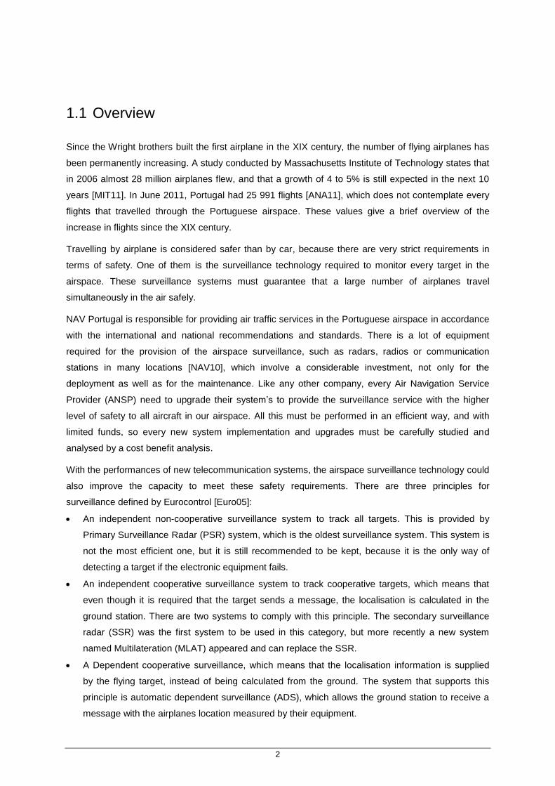
Concerning MLAT and SSR costs, a study was performed by ERA [ERA10] (ERA is a surveillance
system‟s manufacturer). The results provided by the study are shown in Figure 1-2. In terms of costs,
there is a large difference in the acquisition and maintenance price, which will decrease a lot the
expenses for the ANSPs. It shows that in terms of costs, the MLAT solution is better, being one of the
reasons that it will be used in the long term.
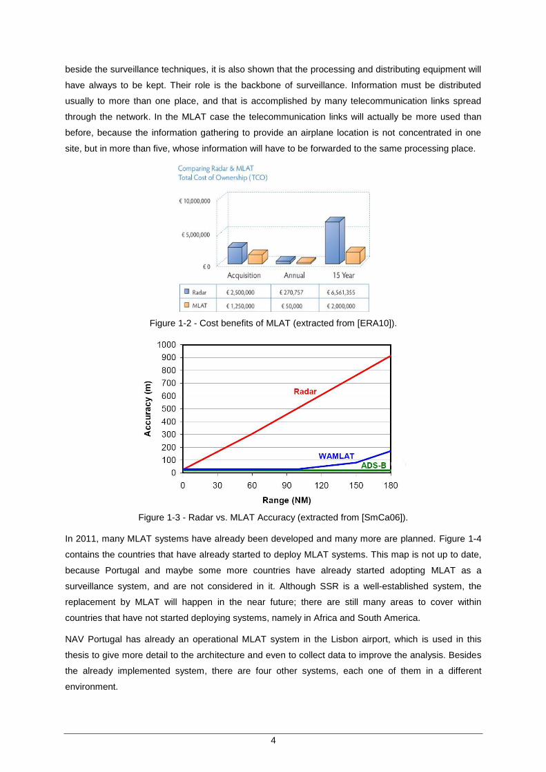
Beside the costs, there are two main characteristics that also give preference to MLAT, the accuracy
of the system for close traffic and safety. According to Figure 1-3, the gain in accuracy is clear
between the SSR (RADAR) and MLAT (WAMLAT). There is also an increase in safety because the
MLAT system by itself is redundant, and even if some parts of the system fail it will continue to work,
unlike SSR that if the radar itself needs to be maintained or fails, the system will stop working.
Another part of the surveillance systems, which is analysed in this thesis, are the communication links
used in air surveillance, which are very important and will have to be used always. In Figure 1-1
4
beside the surveillance techniques, it is also shown that the processing and distributing equipment will
have always to be kept. Their role is the backbone of surveillance. Information must be distributed
usually to more than one place, and that is accomplished by many telecommunication links spread
through the network. In the MLAT case the telecommunication links will actually be more used than
before, because the information gathering to provide an airplane location is not concentrated in one
site, but in more than five, whose information will have to be forwarded to the same processing place.
Figure 1-2 - Cost benefits of MLAT (extracted from [ERA10]).
Figure 1-3 - Radar vs. MLAT Accuracy (extracted from [SmCa06]).
In 2011, many MLAT systems have already been developed and many more are planned. Figure 1-4
contains the countries that have already started to deploy MLAT systems. This map is not up to date,
because Portugal and maybe some more countries have already started adopting MLAT as a
surveillance system, and are not considered in it. Although SSR is a well-established system, the
replacement by MLAT will happen in the near future; there are still many areas to cover within
countries that have not started deploying systems, namely in Africa and South America.
NAV Portugal has already an operational MLAT system in the Lisbon airport, which is used in this
thesis to give more detail to the architecture and even to collect data to improve the analysis. Besides
the already implemented system, there are four other systems, each one of them in a different
environment.

5
The next system to become operational will be in Azores, to cover the central group of islands. This
system is currently in the test phase and is expected to become operational this year. There are two
other projects running; Lisbon Approach Area MLAT project, that is currently on the procurement
phase and another project for Madeira and the North region of Portugal also currently on the
procurement phase.
Figure 1-4 - MLAT implementation worldwide (extracted from [ERA10]).
The main goal of this thesis is to assess the current communication links used in the MLAT systems
owned by NAV Portugal, to help developing the new system that will be implemented in the North
region of Portugal, and to assess the Virtual Private Network connections‟ tolerable delay in the Lisbon
system. To achieve these goals, two simulators were developed, one to analyse the delay in the
communication links and the other to design the coverage in a MLAT system. This last simulator,
besides the individual coverage calculations, also allows overlapping different antennas‟ coverage,
which is useful for technologies that require coverage overlapping, such as MLAT. Finally, the
surveillance requirements were crossed with the MLAT system, to check if the 4 sensors per location
are enough to comply with them.
Although there are many papers concerning different parts of MLAT there are few that analyse entire
systems. This thesis innovation has two parts, in the telecommunication links assessment and in the
system design. The first part considers the analysis of already implemented systems and the overall
magnitude of the delay impact in each type of link to support a MLAT system. The other contribution is
concerning the system design, which analyses some requirements that even though being considered
by manufacturers, their implication has not yet been published.
Also, the coverage simulator has the potential to be used as a tool for developing systems which need
coverage overlapping. There are many coverage simulators in the market, including the one used by
NAV Portugal, which some results are used in this thesis. But there are a few drawbacks because
sometimes, it is not possible to get the intermediate values such has the land profile, the specific
coordinates of the coverage analysis, the overlapping of different coverage maps and finally the paid

6
price.
1.2 Motivation and Contents
“The secret is the soul of business”: this translated Portuguese saying is quite accurate in the
technological business, because technology manufacturers, usually, are not willing to provide very
specific details of their products.
Every ANSP buy the MLAT systems from a manufacturer and, even though manufactures have the
responsibility that the system meets the requirements, it is also important that the ANSP gets some
knowhow of the implemented systems. It is important for working with the system and to judge
critically the implementations proposals of the manufacturers.
The present work is focused in assessing the MLAT telecommunication systems installed by NAV
Portugal and also to provide a preliminary study for a system to be implemented in the North region of
Portugal. In order to assess the telecommunication links, only two aspects were to be analysed, the
required capacity for the links, and their maximum tolerable delay to comply with the MLAT system.
The other main subject of the thesis is to study the coverage requirements of one system, and then to
make a proposal of a possible system configuration to be implemented. A study of the localisation
requirements is completed, and a complete proposal for a new system is presented.
This thesis is composed of 5 chapters, including the present one, and 6 annexes. It is organised in the
following way:
In Chapter 2, one presents an introduction to the existing surveillance systems, including the
technical principals of MLAT. The most common telecommunication links possible to use in a
MLAT system are also described, and finally a state of the art in MLAT.
In Chapter 3, the MLAT architecture and the three developed models for the latency, coverage
analysis and to calculate the maximum latency in a communication link are presented. A
description of both developed simulators based in the latency and coverage model is also
presented. Finally, the MLAT requirements and their implication in the overall system are shown.
In Chapter 4, the results are presented. It includes both results of the simulators, meaning the
expected delays of the current systems and the coverage studies performed for the North region
of Portugal and the results of the maximum tolerable delay for the communication links in a
system to be implemented. Other results are presented that are important to understand this
system, such as the required telecommunication system capacity and how to meet the regulator
recommendations.
The final chapter of the thesis briefly summarizes every conclusion drawn from the work, but also
gives a more global analysis of the problem under study. Finally some recommendations for future
work are given in order to continue developing the MLAT understanding.

7
Chapter 2
Basic Concepts
2 Basic Concepts
This chapter provides an overview of the current status of the air space surveillance systems, giving
more detail to the multilateration systems. A brief description of the telecommunication links more
commonly used in multilateration systems is presented, and the state of the art in this technology is
addressed as well.
8
2.1 Air Space Surveillance
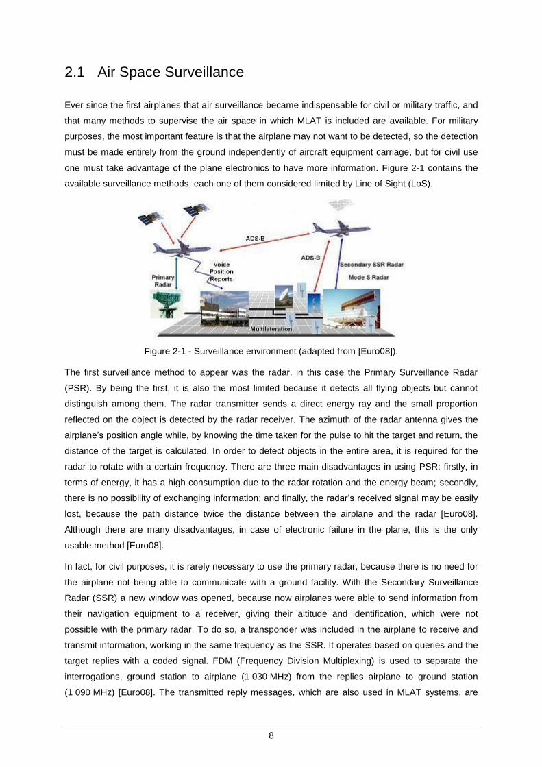
Ever since the first airplanes that air surveillance became indispensable for civil or military traffic, and
that many methods to supervise the air space in which MLAT is included are available. For military
purposes, the most important feature is that the airplane may not want to be detected, so the detection
must be made entirely from the ground independently of aircraft equipment carriage, but for civil use
one must take advantage of the plane electronics to have more information. Figure 2-1 contains the
available surveillance methods, each one of them considered limited by Line of Sight (LoS).
Figure 2-1 - Surveillance environment (adapted from [Euro08]).
The first surveillance method to appear was the radar, in this case the Primary Surveillance Radar
(PSR). By being the first, it is also the most limited because it detects all flying objects but cannot
distinguish among them. The radar transmitter sends a direct energy ray and the small proportion
reflected on the object is detected by the radar receiver. The azimuth of the radar antenna gives the
airplane‟s position angle while, by knowing the time taken for the pulse to hit the target and return, the
distance of the target is calculated. In order to detect objects in the entire area, it is required for the
radar to rotate with a certain frequency. There are three main disadvantages in using PSR: firstly, in
terms of energy, it has a high consumption due to the radar rotation and the energy beam; secondly,
there is no possibility of exchanging information; and finally, the radar‟s received signal may be easily
lost, because the path distance twice the distance between the airplane and the radar [Euro08].
Although there are many disadvantages, in case of electronic failure in the plane, this is the only
usable method [Euro08].
In fact, for civil purposes, it is rarely necessary to use the primary radar, because there is no need for
the airplane not being able to communicate with a ground facility. With the Secondary Surveillance
Radar (SSR) a new window was opened, because now airplanes were able to send information from
their navigation equipment to a receiver, giving their altitude and identification, which were not
possible with the primary radar. To do so, a transponder was included in the airplane to receive and
transmit information, working in the same frequency as the SSR. It operates based on queries and the
target replies with a coded signal. FDM (Frequency Division Multiplexing) is used to separate the
interrogations, ground station to airplane (1 030 MHz) from the replies airplane to ground station
(1 090 MHz) [Euro08]. The transmitted reply messages, which are also used in MLAT systems, are
9
Modes A and C (Mode A/C) [Nav08]. With SSR, the distance between the radar and the airplane is
calculated by the time difference between the interrogation and reply message. Adding this
information to the altitude reports the airplane 3D position is known. This position is updated on every
radar sweep, having a period in [4, 12] s, depending on the radar [Era10].
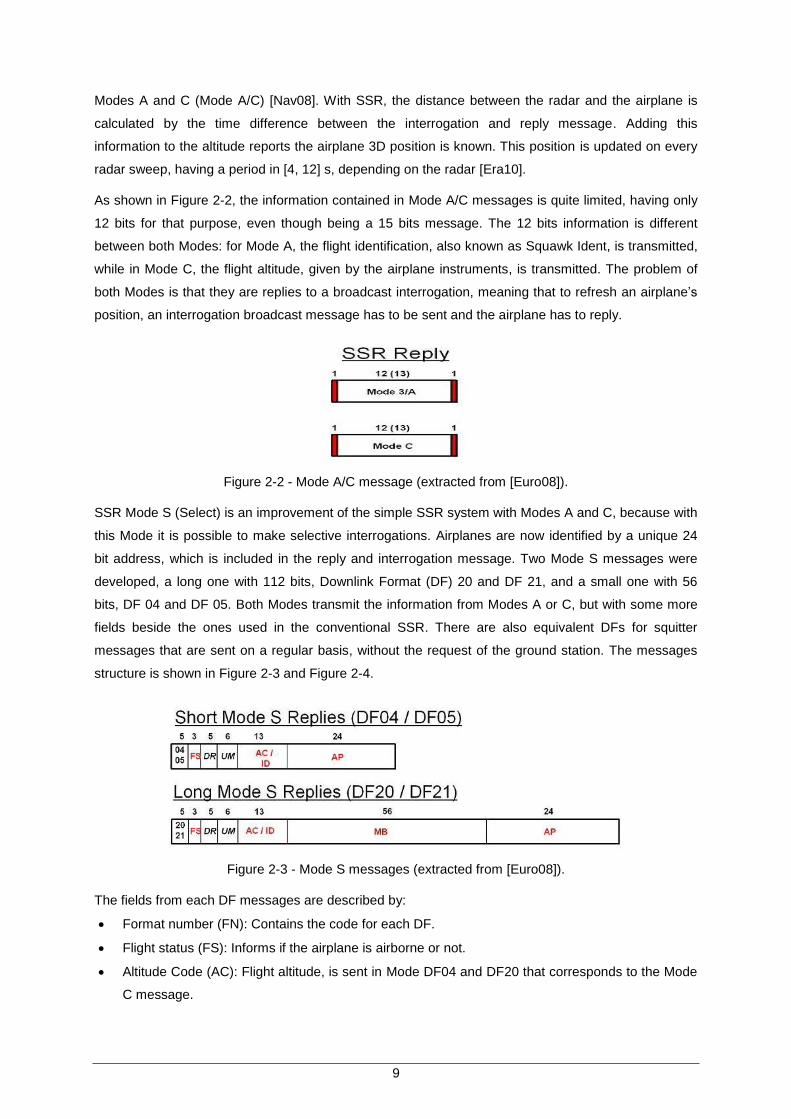
As shown in Figure 2-2, the information contained in Mode A/C messages is quite limited, having only
12 bits for that purpose, even though being a 15 bits message. The 12 bits information is different
between both Modes: for Mode A, the flight identification, also known as Squawk Ident, is transmitted,
while in Mode C, the flight altitude, given by the airplane instruments, is transmitted. The problem of
both Modes is that they are replies to a broadcast interrogation, meaning that to refresh an airplane‟s
position, an interrogation broadcast message has to be sent and the airplane has to reply.
Figure 2-2 - Mode A/C message (extracted from [Euro08]).
SSR Mode S (Select) is an improvement of the simple SSR system with Modes A and C, because with
this Mode it is possible to make selective interrogations. Airplanes are now identified by a unique 24
bit address, which is included in the reply and interrogation message. Two Mode S messages were
developed, a long one with 112 bits, Downlink Format (DF) 20 and DF 21, and a small one with 56
bits, DF 04 and DF 05. Both Modes transmit the information from Modes A or C, but with some more
fields beside the ones used in the conventional SSR. There are also equivalent DFs for squitter
messages that are sent on a regular basis, without the request of the ground station. The messages
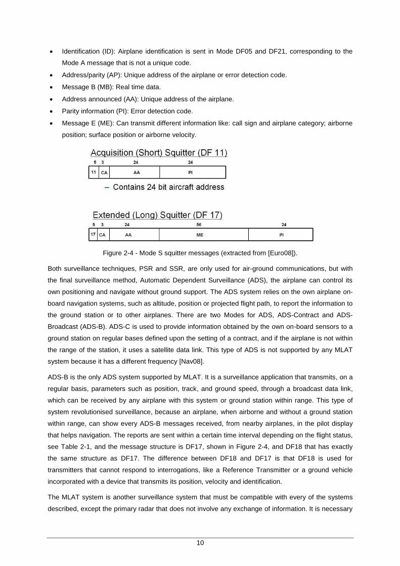
structure is shown in Figure 2-3 and Figure 2-4.
Figure 2-3 - Mode S messages (extracted from [Euro08]).
The fields from each DF messages are described by:
Format number (FN): Contains the code for each DF.
Flight status (FS): Informs if the airplane is airborne or not.
Altitude Code (AC): Flight altitude, is sent in Mode DF04 and DF20 that corresponds to the Mode
C message.
10
Identification (ID): Airplane identification is sent in Mode DF05 and DF21, corresponding to the
Mode A message that is not a unique code.
Address/parity (AP): Unique address of the airplane or error detection code.
Message B (MB): Real time data.
Address announced (AA): Unique address of the airplane.
Parity information (PI): Error detection code.
Message E (ME): Can transmit different information like: call sign and airplane category; airborne
position; surface position or airborne velocity.
Figure 2-4 - Mode S squitter messages (extracted from [Euro08]).
Both surveillance techniques, PSR and SSR, are only used for air-ground communications, but with
the final surveillance method, Automatic Dependent Surveillance (ADS), the airplane can control its
own positioning and navigate without ground support. The ADS system relies on the own airplane on-
board navigation systems, such as altitude, position or projected flight path, to report the information to
the ground station or to other airplanes. There are two Modes for ADS, ADS-Contract and ADS-
Broadcast (ADS-B). ADS-C is used to provide information obtained by the own on-board sensors to a
ground station on regular bases defined upon the setting of a contract, and if the airplane is not within
the range of the station, it uses a satellite data link. This type of ADS is not supported by any MLAT
system because it has a different frequency [Nav08].
ADS-B is the only ADS system supported by MLAT. It is a surveillance application that transmits, on a
regular basis, parameters such as position, track, and ground speed, through a broadcast data link,
which can be received by any airplane with this system or ground station within range. This type of
system revolutionised surveillance, because an airplane, when airborne and without a ground station
within range, can show every ADS-B messages received, from nearby airplanes, in the pilot display
that helps navigation. The reports are sent within a certain time interval depending on the flight status,
see Table 2-1, and the message structure is DF17, shown in Figure 2-4, and DF18 that has exactly
the same structure as DF17. The difference between DF18 and DF17 is that DF18 is used for
transmitters that cannot respond to interrogations, like a Reference Transmitter or a ground vehicle
incorporated with a device that transmits its position, velocity and identification.
The MLAT system is another surveillance system that must be compatible with every of the systems
described, except the primary radar that does not involve any exchange of information. It is necessary
11
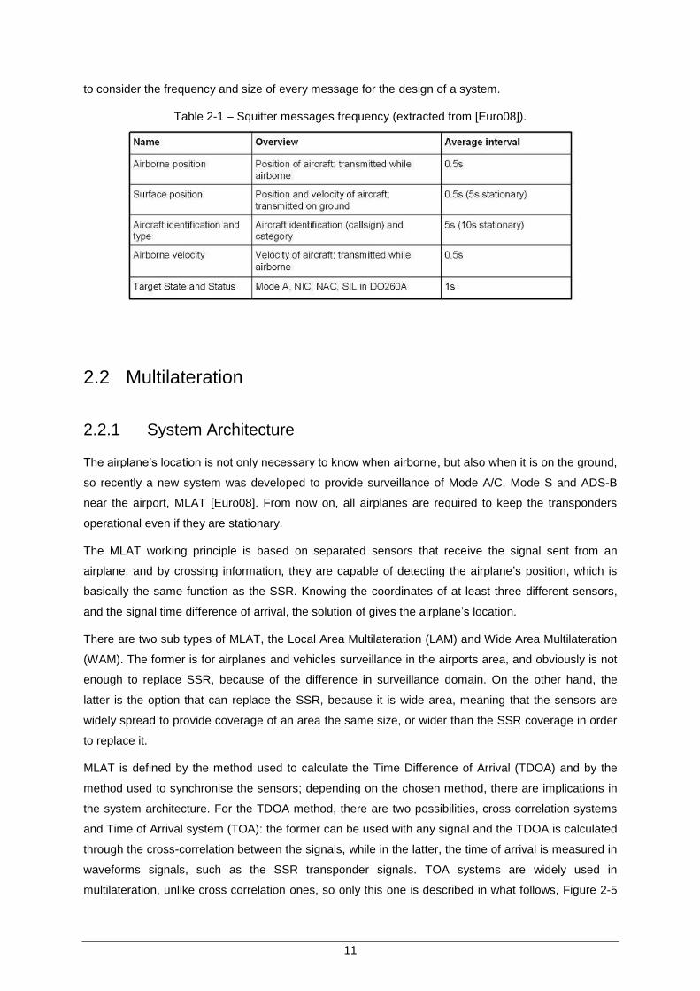
to consider the frequency and size of every message for the design of a system.
Table 2-1 – Squitter messages frequency (extracted from [Euro08]).
2.2 Multilateration
2.2.1 System Architecture
The airplane‟s location is not only necessary to know when airborne, but also when it is on the ground,
so recently a new system was developed to provide surveillance of Mode A/C, Mode S and ADS-B
near the airport, MLAT [Euro08]. From now on, all airplanes are required to keep the transponders
operational even if they are stationary.
The MLAT working principle is based on separated sensors that receive the signal sent from an
airplane, and by crossing information, they are capable of detecting the airplane‟s position, which is
basically the same function as the SSR. Knowing the coordinates of at least three different sensors,
and the signal time difference of arrival, the solution of gives the airplane‟s location.
There are two sub types of MLAT, the Local Area Multilateration (LAM) and Wide Area Multilateration
(WAM). The former is for airplanes and vehicles surveillance in the airports area, and obviously is not
enough to replace SSR, because of the difference in surveillance domain. On the other hand, the
latter is the option that can replace the SSR, because it is wide area, meaning that the sensors are
widely spread to provide coverage of an area the same size, or wider than the SSR coverage in order
to replace it.
MLAT is defined by the method used to calculate the Time Difference of Arrival (TDOA) and by the
method used to synchronise the sensors; depending on the chosen method, there are implications in
the system architecture. For the TDOA method, there are two possibilities, cross correlation systems
and Time of Arrival system (TOA): the former can be used with any signal and the TDOA is calculated
through the cross-correlation between the signals, while in the latter, the time of arrival is measured in
waveforms signals, such as the SSR transponder signals. TOA systems are widely used in
multilateration, unlike cross correlation ones, so only this one is described in what follows, Figure 2-5
12
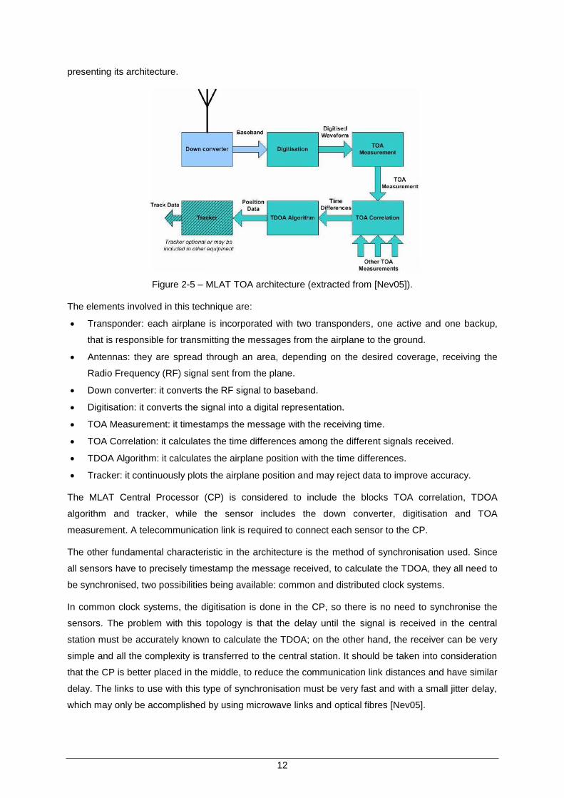
presenting its architecture.
Figure 2-5 – MLAT TOA architecture (extracted from [Nev05]).
The elements involved in this technique are:
Transponder: each airplane is incorporated with two transponders, one active and one backup,
that is responsible for transmitting the messages from the airplane to the ground.
Antennas: they are spread through an area, depending on the desired coverage, receiving the
Radio Frequency (RF) signal sent from the plane.
Down converter: it converts the RF signal to baseband.
Digitisation: it converts the signal into a digital representation.
TOA Measurement: it timestamps the message with the receiving time.
TOA Correlation: it calculates the time differences among the different signals received.
TDOA Algorithm: it calculates the airplane position with the time differences.
Tracker: it continuously plots the airplane position and may reject data to improve accuracy.
The MLAT Central Processor (CP) is considered to include the blocks TOA correlation, TDOA
algorithm and tracker, while the sensor includes the down converter, digitisation and TOA
measurement. A telecommunication link is required to connect each sensor to the CP.
The other fundamental characteristic in the architecture is the method of synchronisation used. Since
all sensors have to precisely timestamp the message received, to calculate the TDOA, they all need to
be synchronised, two possibilities being available: common and distributed clock systems.
In common clock systems, the digitisation is done in the CP, so there is no need to synchronise the
sensors. The problem with this topology is that the delay until the signal is received in the central
station must be accurately known to calculate the TDOA; on the other hand, the receiver can be very
simple and all the complexity is transferred to the central station. It should be taken into consideration
that the CP is better placed in the middle, to reduce the communication link distances and have similar
delay. The links to use with this type of synchronisation must be very fast and with a small jitter delay,
which may only be accomplished by using microwave links and optical fibres [Nev05].

13
Figure 2-6 - Common clock system architecture (extracted from [Nev05]).
Finally, in the distributed clock system, receivers are more complex, because they need to handle the
digitisation and timestamp before forwarding the message to the CP, but on the other hand there is
much more flexibility for the communication link, because they support a much higher delay. The main
disadvantage is that it is required to use a synchronisation technique for the sensors clock, which can
be: transponder synchronised system; standalone Global Navigation Satellite System (GNSS)
synchronised system; and common view GNSS synchronised system. Independently from the
synchronisation technique, the architecture is always the same, as in Figure 2-7. The function of the
synchronisation technique is to assure that all local clocks have the same time base.
Figure 2-7 - Distributed clock system architecture (extracted from [Nev05]).
According to the chosen system architecture, there are different requirements to the communication
links between the sensors and the CP. In the case of a common clock system, the links must all have
the minimum latency possible, so one should use fibre or microwave links, while with distributed clock
systems, there are no latency requirements, because the timestamp has already occurred. Even
though latency is not critical, it must be assured that the latency between the fastest and slowest links
does not exceed a certain value, due to the MLAT processor constrains [Nev05].
14
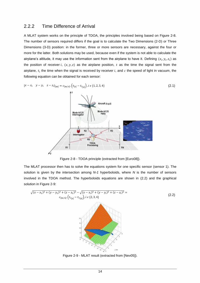
2.2.2 Time Difference of Arrival
A MLAT system works on the principle of TDOA, the principles involved being based on Figure 2-8.
The number of sensors required differs if the goal is to calculate the Two Dimensions (2-D) or Three
Dimensions (3-D) position: in the former, three or more sensors are necessary, against the four or
more for the latter. Both solutions may be used, because even if the system is not able to calculate the
airplane‟s altitude, it may use the information sent from the airplane to have it. Defining as
the position of receiver , as the airplane position, as the time the signal sent from the
airplane, the time when the signal is received by receiver , and the speed of light in vacuum, the
following equation can be obtained for each sensor:
(2.1)
Figure 2-8 - TDOA principle (extracted from [Euro08]).
The MLAT processor then has to solve the equations system for one specific sensor (sensor 1). The
solution is given by the intersection among N-1 hyperboloids, where N is the number of sensors
involved in the TDOA method. The hyperboloids equations are shown in (2.2) and the graphical
solution in Figure 2-9:
, (2.2)
Figure 2-9 - MLAT result (extracted from [Nev05]).

15
The solution of this system gives the airplane‟s position, but there is an error associated to the
process, due to the error in the time-stamping, because sensors are not exactly synchronised. This
error would increase if there was no time-stamping, because the accuracy of detecting the difference
in propagation times in each link is smaller than the synchronisation accuracy. The more sensors
involved in the process, the higher the system accuracy is [Euro08]. According to [Nev05], with a
specific distribution of sensors, it is possible to achieve the SSR accuracy with only five sensors.
2.3 Telecommunications Systems Supporting Multilateration
2.3.1 Introduction
The telecommunication system to use depends on the requirements of the service for which it is
supporting. In the case of MLAT it is shown if a certain feature of the telecommunication system is
important or not. The characteristics to be evaluated are:
Capacity: It is the most important feature of the majority of the systems, but concerning MLAT, it is
one of the least important, because the exchanged messages are not very large and the required
capacity is not very high. Even so, the maximum traffic of messages should be calculated to know
the minimum capacity of the telecommunication link.
Latency: It is the total time of the message to get from the airplane to the CP. It contains a system
delay component, a delay in the telecommunication link, and the delay over air. It must be assured
that the latency in the system does not exceed a certain value, and that the difference between
the fastest and slowest sensors is lower than a certain time.
Fading: It is a problem present in radio link communication channels. Although it does not happen
in optical fibres, if one considers microwave links, it is necessary to take it into consideration.
Distance: It is important to know the maximum distances achievable with each kind of link,
because in the case of WAM link lengths may be quite large.
The goal of studying the communication links is to know which are the limitations or advantages in the
possible systems to study. One considers optical fibres, microwave links, satellite links, and Virtual
Private Networks (VPN).
2.3.2 Optical Fibre
The telecommunications system most used nowadays are optical fibres, because it is the type of
communication link with the highest bit rates and less errors. The bit rate depends on the fibre and
laser used, but the rates are much above the one that is required by a MLAT system. The
communication channel, depends mostly on the fibre modes, it being either Single Mode Fibre (SMF)
or Multi Mode Fibre (MMF).
Initially, MMF was used, since by having a larger core it is easier to inject the signal, hence, working

16
with worse lasers. MMFs support data rates from 10 Mbps up to 10 Gbps, with standards in
development to support up to 100 Gbps [FOLS08]. The limitation in a fibre is given by the losses or
the modal dispersion. The standards currently defined for MMF from ISO/IEC 11802 specifications are
OM1 to OM4, and the values for the maximum attenuation and minimum modal bandwidth are given
by the Table 2-2 [FIA10] and [FIA08].
Table 2-2 – OM standards.
Category
Maximum Attenuation
Minimum modal bandwidth
Maximum distance @ 100Mbs
Attenuation for the
maximum distance
LED Laser LED Laser LED Laser
850 nm
1300 nm
850 nm
1300 nm
850 nm
850 nm
1300 nm
850 nm
850 nm
1300 nm
850 nm
OM1 3.5 1.5 200 500 N/A 02 5 N/A 7 7.5 N/A
OM2 3.5 1.5 500 500 N/A 05 5 N/A 17.5 7.5 N/A
OM3 3.5 1.5 1500 500 2000 15 5 20 52.5 7.5 700
OM4 30 10 3500 500 4700 35 5 47 105 50 141
The minimal modal bandwidth imposes a maximum distance for a given transmission rate, which is
shown in the previous table, based on:
(2.3)
where:
: Maximum fibre length.
: Modal bandwidth.
: Transmission rate.
In the case of SMF, the core is smaller, having less dispersion than in the MMF. The limitation in this
fibre is also from the fibre losses, but not from the modal dispersion, because there is only one mode
propagating, so the other limitation is the chromatic dispersion. ISO/IEC 11801 specifies OS1 and
ISO/IEC 24702 specify OS2, which have defined the maximum values for attenuation, shown in Table
2-3.
Table 2-3 - OS Standards (adapted from [FIA08]).
Wavelength Maximum attenuation
OS1 OS2
1310 1.0 0.4
1385 Not specified 0.4
1550 1.0 0.4

17
Recent SMFs have chromatic dispersion compensation, so the limitation is only given by the fibre
attenuation, which is imposed by the laser power, receiver sensitivity, and system margin.
Beside the fibre losses there are extra attenuations to be considered, the connector losses and splice
losses that are used to connect different fibre sections to achieve higher lengths. Each element losses
depend on the manufacturer, but there are maximum values recommended by the International
Telecommunication Union - Telecommunication (ITU-T) shown in Table 2-4, the total losses being:
(2.4)
where:
: Total path losses.
: Attenuation coefficient with distance.
: Link length.
: Number of connectors.
: Connector losses.
: Number of splices.
: Splice losses.
Table 2-4 - Optical elements recommended loss (adapted from [ITUT09])
Attenuation coefficient Typical link value
Splice Maximum 0.5
Connector for SMF Maximum 0.5
Connector for MMF Maximum 1.0
The total latency for an optical fibre is given by [FOIA08]:
(2.5)
where:
: Total link delay.
: Transmission time.
: Propagation delay.
: Random jitter delay
: Fixed delay.
Propagation delay is a characteristic that is of no concern, because the propagation speed can be
roughly approximated by the speed of light divided by the optical index of the glass ( ), which is
fast enough for any system one may consider. Transmission time depends on the fibre transmission
rate and the message volume ( ), being given by:
(2.6)
The major disadvantage of the fibre is the civil construction to install the cables, especially with a
18
point-to-point topology, which involves digging to protect the cables. Concerning capacity, distance
and delay limitations, there are not any with this type of telecommunication link.
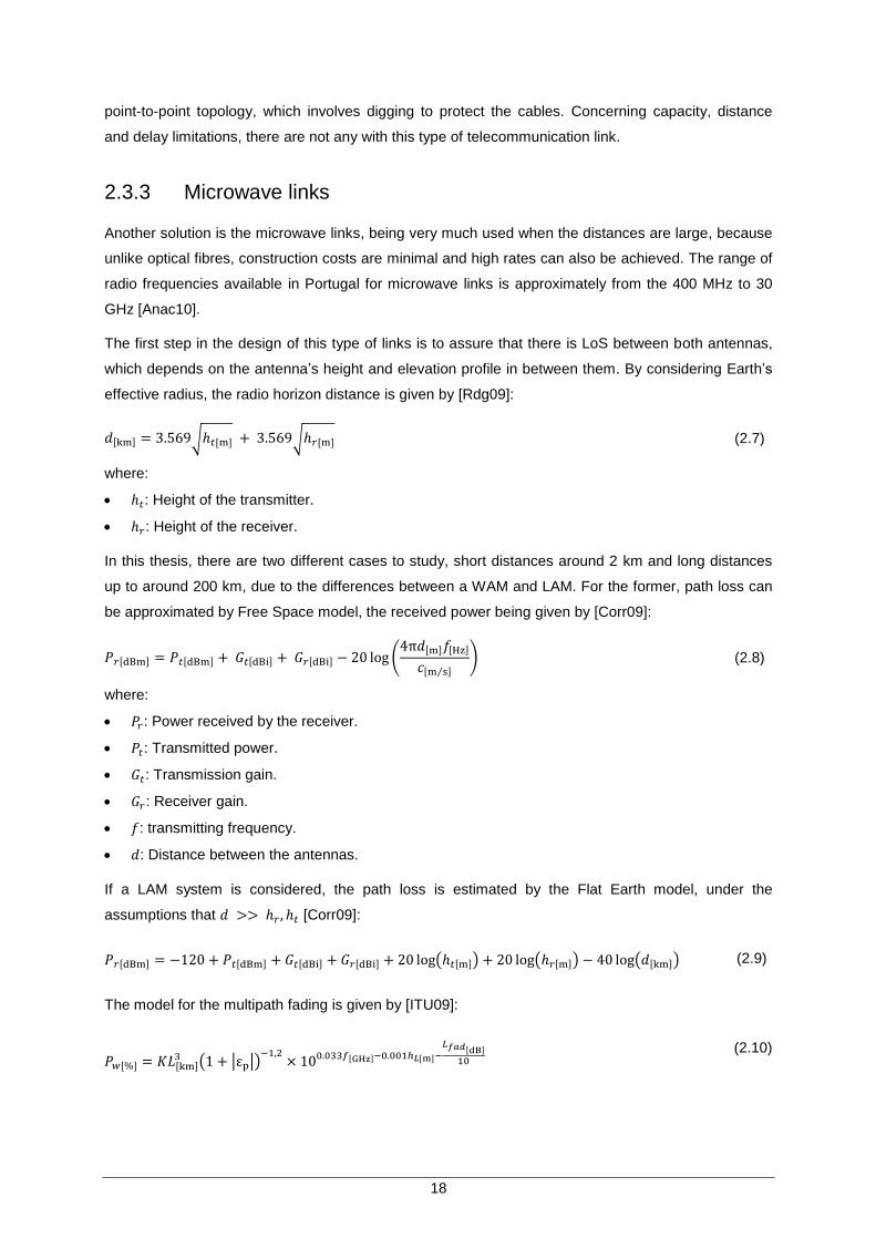
2.3.3 Microwave links
Another solution is the microwave links, being very much used when the distances are large, because
unlike optical fibres, construction costs are minimal and high rates can also be achieved. The range of
radio frequencies available in Portugal for microwave links is approximately from the 400 MHz to 30
GHz [Anac10].
The first step in the design of this type of links is to assure that there is LoS between both antennas,
which depends on the antenna‟s height and elevation profile in between them. By considering Earth‟s
effective radius, the radio horizon distance is given by [Rdg09]:
(2.7)
where:
: Height of the transmitter.
: Height of the receiver.
In this thesis, there are two different cases to study, short distances around 2 km and long distances
up to around 200 km, due to the differences between a WAM and LAM. For the former, path loss can
be approximated by Free Space model, the received power being given by [Corr09]:
(2.8)
where:
: Power received by the receiver.
: Transmitted power.
: Transmission gain.
: Receiver gain.
: transmitting frequency.
: Distance between the antennas.
If a LAM system is considered, the path loss is estimated by the Flat Earth model, under the
assumptions that [Corr09]:
(2.9)
The model for the multipath fading is given by [ITU09]:
(2.10)
19
(2.11)
(2.12)
where:
: Probability of exceeding the attenuation value.
: Climate parameter.
: Path inclination.
: Maximum fading attenuation.
: Lowest height between the receiver and transmitter.
: Refractivity lapse rate in the first 65 m not exceeded for 1% of the year ( in
Portugal) [ITU03].
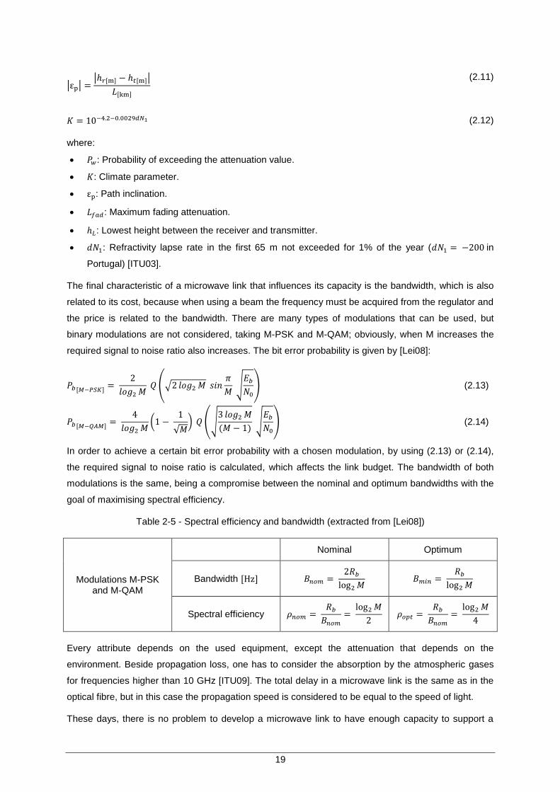
The final characteristic of a microwave link that influences its capacity is the bandwidth, which is also
related to its cost, because when using a beam the frequency must be acquired from the regulator and
the price is related to the bandwidth. There are many types of modulations that can be used, but
binary modulations are not considered, taking M-PSK and M-QAM; obviously, when M increases the
required signal to noise ratio also increases. The bit error probability is given by [Lei08]:
(2.13)
(2.14)
In order to achieve a certain bit error probability with a chosen modulation, by using (2.13) or (2.14),
the required signal to noise ratio is calculated, which affects the link budget. The bandwidth of both
modulations is the same, being a compromise between the nominal and optimum bandwidths with the
goal of maximising spectral efficiency.
Table 2-5 - Spectral efficiency and bandwidth (extracted from [Lei08])
Modulations M-PSK and M-QAM
Nominal Optimum
Bandwidth
Spectral efficiency
Every attribute depends on the used equipment, except the attenuation that depends on the
environment. Beside propagation loss, one has to consider the absorption by the atmospheric gases
for frequencies higher than 10 GHz [ITU09]. The total delay in a microwave link is the same as in the
optical fibre, but in this case the propagation speed is considered to be equal to the speed of light.
These days, there is no problem to develop a microwave link to have enough capacity to support a
20
MLAT system. Concerning the distances involved in a WAM system, the microwave link is also
enough, because even without LoS or with a too long path, repeaters may be used.
2.3.4 Satellite Link and Virtual Private Network
In case it is difficult to implement a proprietary solution, it is possible to rent one from any service
provider with a network in the area. Abstracting from the system description itself, when a
communication link is rented there are advantages and disadvantages. The advantages are that there
is no need to design the communication link, not to maintain it, and investment capital is saved by not
constructing the system. On the other hand, there are two main disadvantages: the service is
contracted and needs to be paid for the leased time and bandwidth, as long as the system is working;
the latency must be negotiated with the service provider in order to guarantee the required values.
These links are usually satellite systems and VPNs.
There are three types of circular satellite orbits: Geosynchronous orbit (GEO), Medium Earth Orbit
(MEO) and Low Earth Orbit (LEO), which the respectively altitudes are 35 786 km, [8 000, 20 000] km
and [500, 2 000] km [ISAT11]. The communication frequencies for fixed satellite communications in
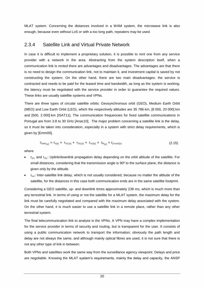
Portugal are from 3.8 to 30 GHz [Anac10]. The major problem concerning a satellite link is the delay,
so it must be taken into consideration, especially in a system with strict delay requirements, which is
given by [Emm00].
(2.15)
where
and : Uplink/downlink propagation delay depending on the orbit altitude of the satellite. For
small distances, considering that the transmission angle is 90º to the surface plane, the distance is
given only by the altitude.
: Inter-satellite link delay, which is not usually considered, because no matter the altitude of the
satellite, for the distances in this case both communication ends are in the same satellite footprint.
Considering a GEO satellite, up- and downlink times approximately 238 ms, which is much more than
any terrestrial link. In terms of using or not the satellite for a MLAT system, the maximum delay for the
link must be carefully negotiated and compared with the maximum delay associated with the system.
On the other hand, it is much easier to use a satellite link in a remote place, rather than any other
terrestrial system.
The final telecommunication link to analyse is the VPNs. A VPN may have a complex implementation
for the service provider in terms of security and routing, but is transparent for the user. It consists of
using a public communication network to transport the information; obviously the path length and
delay are not always the same, and although mainly optical fibres are used, it is not sure that there is
not any other type of link in between.
Both VPNs and satellites work the same way from the surveillance agency viewpoint. Delays and price
are negotiable. Knowing the MLAT system‟s requirements, mainly the delay and capacity, the ANSP
21
will have to guarantee them. The main difference between them is the price and the capacity available
in both types of links. If there is the possibility of using a VPN, it should certainly be used, because of
the smaller price and delay for the same capacity.
2.4 State of the art
Nowadays, MLAT is a surveillance technique that is being worldwide used, but still studies are being
conducted to get more knowledge concerning this technique. This section intends to show the
research that has been done in the past and what is being done now, in manly four areas: sensors
synchronisation, algorithm for the TDOA, accuracy of the system, and sensors location.
The basis for the MLAT is the TDOA algorithm, which has been improving since the late 1980s when
Smith and Abel in [SmAb87] proposed the spherical interpolated method. Many other methods have
been proposed since, such as Chain and Ho in [ChHo94] or Savage et. al. in [SaCr06]. Still, the
research in better and more efficient localisation algorithms is being performed with numerous articles.
Every manufacturer has its own TDOA algorithm, which may differ a lot from each other and also
influence the accuracy of the system.
There are studies, such as [BoZh10], which try to maximise the coverage for a given accuracy using
genetic algorithms, but the main disadvantage is that in a real system, the localisation also depends
on the construction site. To synchronise the sensors, if required, there are many ways of achieving it
as discussed in Section 2.2.1. The two approaches more used are by using reference transmitters or
satellite, the latter being recommended to use with more dispersed sensors [Chao09].
[Nev05] is a complete report to analyse the advantages and disadvantages of MLAT, and how to
achieve a service equivalent to the SSR. They state that with five sensors the same accuracy as the
SSR is achieved, among other information such as:
The best signals to use in MLAT, which are the signals explained in this thesis.
Possible synchronisation methods and their classification in terms of accuracy.
Accuracy for specific sensor‟s geometrical configurations.
Best way to choose the receivers.
With the development of the mathematical concepts behind MLAT, the improvement of the MLAT
system itself has been mainly driven by MLAT manufacturers, the European Organisation for the
Safety of Air Navigation (Eurocontrol), and the European Organisation for Civil Aviation Equipment
(Eurocae). Most of the research available concerns test pilots performed in many different countries,
and the advantages of adopting MLAT instead of the SSR. In October 2009, Eurocontrol published a
press release, in [Euro09], after a workshop with an international group of experts stating, “Wide Area
Multilateration – A surveillance technique that is ready for use”.
There are four manufactures with implementation experience, Era, Roke Manor, Indra Systems, and
22
Sensis Corporation. All of these companies have experience developing any MLAT system for any
region or airport (WAM or LAM). The main disadvantage is that when developing a new system, the
ANSP may not be prepared to evaluate the planning in a critical way. On the other hand, all the
responsibility to achieve the requirements is on the manufacturer‟s side, which has to be guaranteed.

23
Chapter 3
Models and Simulators
3 Models and Simulators
This chapter provides the description of the latency and coverage simulator and the associated
models. Other models to assess a MLAT system are also described despite not being used in the
simulators.
24
3.1 NAV Portugal Multilateration Systems
3.1.1 System Architecture
In Section 2.2, a general description of the MLAT algorithm and the sensors synchronisation has been
presented. In a real MLAT system, there are many more components to provide basic functionalities
that are not referenced in the theoretical analysis. This chapter intends to describe the top level
architecture for the MLAT system installed in the Lisbon airport.
Figure 3-1 contains the current system installed in the Lisbon airport. There are four main components
of the system, the transponders to equip the aircrafts or ground vehicles, the Remote Units (RUs) or
sensors, the reference transmitters, and the Central Processing System (CPS), that contains the CP.
All the components in the system are redundant, because in a critical system the hardware must be
redundant in order to avoid single failures.
The first main component of the system is the transponder incorporated in the airplane or ground
vehicle. This transponder is the communication equipment of the airplane that receives and transmits
the surveillance messages, which for this system are Mode A/C, Mode S and ADS-B. In the case of
the airplane, the transponder contains two antennas, one at the top and the other at the bottom. When
airborne it uses both antennas alternately, while when on the ground the default transponder is the
one on the top. The justification for using both antennas when airborne is mainly because sometimes,
when changing routes, the bottom antenna can lose LoS for the receivers, so with both it is guarantee
that at least one of them is at LoS.
RUs work as sensors in a MLAT system. Each RU can be configured as a receiver or transceiver:
when acting as a receiver, it receives, decodes and timestamps Mode A/C, Mode S and ADS-B
replies, while as a transceiver, it can also transmit 1030MHz interrogations. In addition, it has two
more important capabilities, GPS interface and communication interface. The GPS interface is
optional, but when used, the RU is able to receive time information signals and use them for time
synchronisation. The communication interface connects the RU to the CP, via and communication
system. In this specific case, only optical fibres are used [Sns09b].
The third main component is the Reference Transmitters (reftrans), which are responsible for the time
synchronisation of the sensors. Instead of using GPS synchronisation, reftrans transmit DF 18 squitter
messages at a rate of approximately one per second. DF 18 messages have exactly the same
structure of DF 17 in Figure 2-4, but it is also used for a ground vehicle. It is through these messages
that synchronisation is achieved.
Finally, there is the CPS, which is an Ethernet-based Local Area Network (LAN) with communication
and data processing equipment. Data is collected from the different sensors and distributed three-
ways, so that the target position is calculated and displayed. Two data streams are forward to the
primary and secondary operational system, while the third stream is used for a test system.

25
Figure 3-1 - System Architecture Lisbon (extracted from [Sns09c]).
26
Even though there are two operational systems, they are equivalent, since both simultaneously
process replies; the only difference between them, if no failure is reported, is that only the primary
system provides output reports. When detected any failure in the primary system, the secondary
assumes the role of primary. As shown in Figure 3-1, the main components of the CPS are:
Target Processor (TP), processes the sensor replies, which means calculating the three
dimensional position based on the TDOA algorithm.
Maintenance Display Terminal (MDT) provides display, such as, target positions, statistics, data
recording and system archival. Sensors in normal operating mode are controlled through this
component. There are two MDTs, one local and another for remote access.
Cisco Smart Switch multiplexes data from every sensor to the correspondent TP.
HP Switch is used for internal communication between the TPs and MDTs. Internet Group
Management Protocol has been enabled in these switches for correct handling of multicast data.
There is one last component of the system outside the CPS, which is the eLCMS (embedded Local
Control Monitoring System) that provides fault diagnostics and local control over the RUs.
To avoid failures in the operative system, the test system was also implemented to evaluate the
impact of any changes or to test any possible improvement before executing it on the operational
systems. The test system shares the Cisco Smart Switch with the primary target processor, but
besides that, has an independent system with its own TP, HP Switch and MDT. Any RU can be
controlled by the test MDT, but then it stays offline for the operational system‟s MDT so that any
change does not impact the on operational system.
3.1.2 Support Communication System
Sensors are spread through the terrain, and to connect each one of them to the CP, a
telecommunication link is required for each of them. In the Lisbon LAM it was chosen to use a point-to-
point topology with two optical fibres per sensor, each one for a communication link, uplink and
downlink. There were two options available for the fibres, SMF and MMF. Table 3-1 contains the
description of both types of fibres, but in the Lisbon system only SMFs were used. Instead of optical
fibres, any other communication link could have been chosen. The latency specifications are that the
latency between the fastest and slowest link does not exceed 500 ms.
The information exchanged in the fibre lines between the RUs and the TP is typically Internet Protocol
(IP) with a connection-less scheme; besides the message itself, it is added the IP header, User
Datagram Protocol (UDP) header, Internet Group Management Protocol version 2 (IGMP v2) header
and finally the Ethernet frame header, the specific values of the overheads being shown in Table 3-2
[Nav11]. It must be noticed that other headers can be used by different manufacturers.
As explained in Chapter 2, squitter messages have a minimum rate in messages per second that also
depends on the airplane or vehicle positions. For the specific system implemented in Lisbon, the
different messages rate corresponding to the different formats available are given by Table 3-3
[Nav11]. The types of messages inherited from SSR, Mode A/C and Mode S, do not have a fixed

27
sending frequency, but if this system is a real substitution of the SSR, it means that it has to achieve at
least the highest frequency of the previous system. Taking into consideration that the SSR could only
make an interrogation on each rotation period for each airplane, and having a rotation period of 4 s the
frequency of this SSR is considered 0.25 messages per second.
Table 3-1 - SMF/MMF Specifications and Standards (adapted from [Sns09b])
Specification/Standard SMF Description MMF Description
Output Ethernet over Fibre Ethernet over Fibre
Fibre Cable 9 50/62.5
Max Distance 10 2
Max Data Rate 100 100
Table 3-2 – Overheads in MLAT messages
Header Overhead [Bytes]
Ethernet Frame 14
IP 20
UDP 08
IGMP v2 08
Total Overhead 50
Table 3-3 - Exchanged messages rates and sizes [NAV11]
Surveillance System
Downlink Format
Transmitted Information Size
Size with overhead
Frequency
ADS-B
DF17 Position or velocity updates 14 64 Moving: 4 Stationary: 0.2
DF17 Airplane identification and callsign
14 64 0.2
DF18 Position or velocity updates for a vehicle or RefTrans
14 64 Moving: 4 Stationary: 0.2
DF11 Airplane address 07 57 Airborne: 1
Mode S
DF4/DF5 Airplane identification or altitude code
07 57 0.25
DF20/
DF21
Airplane identification or altitude code plus real-time data reports
14 64 0.25
Before the model implementation, and to analyse values given by the manufacturer, it is necessary to
calculate some parameters that are directly related to the communication system, such as the rate and
volume of the exchanged messages. These variables depend on the number of airplanes at range, the
traffic generated, and size of the exchanged messages. The system must guarantee at least 250
airplanes or vehicles simultaneously [NAV08] and the different message sizes and frequencies that
they are sent are shown in Table 3-3. The following equations are defined to calculate the expected
traffic:

28
(3.1)
(3.2)
where:
: Average traffic for Mode S messages transmitting Mode A/C information.
: Average traffic for ADS-B.
: Number of airplanes at range.
: Number of vehicles.
: Average message arrival rate per airplane for long Mode S.
: Average message arrival rate per airplane for short Mode S.
: Average message arrival rate per airborne target for ADS-B.
: Average message arrival rate per moving target for ADS-B.
: Average message arrival rate per stationary target for ADS-B.
: Ratio of targets airborne.
: Ratio of targets moving.
: Ratio of targets stationary.
: Size of short Mode S messages.
: Size of long Mode S messages equivalent to ADS-B.
The capacity estimation also depends on the area each sensor covers and theirs receiving probability.
To study the coverage of each sensor, it is necessary to analyse the intersection between the sensor‟s
coverage areas with the MLAT area. Concerning the receiving probability, it obviously reduces the
traffic expected in the link, but also decreases the probability of the success of the TDOA algorithm,
because to have a successful localisation in the CP, 4 sensors must receive the message.
3.1.3 Localisation Requirements
There are always standard requirements in a surveillance system, especially in the airplane probability
of detection. The requirements for this system in terms of probability of detection are defined by
Eurocae [NAV11]:
Track Initiation: it is defined as the time from when an airplane enters the operational coverage
area to the output of the first position from the MLAT system.
Continuous tracking: it is defined as the time between two consecutives position updates.
From the Eurocae recommendations, the track initiation shall be less or equal to 5 times the defined
update interval with the probability of 99%, and the continuous tracking less or equal to the update
interval with the probability of 97%. For the continuous tracking, only one successful MLAT position is
required, but for the track initiation two or three consecutive ones are required. The update interval for
the WAM system is 5 s [NAV11].
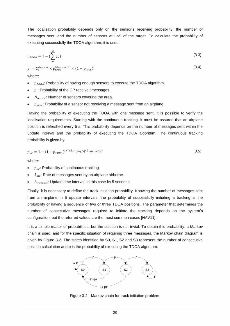
29
The localisation probability depends only on the sensor‟s receiving probability, the number of
messages sent, and the number of sensors at LoS of the target. To calculate the probability of
executing successfully the TDOA algorithm, it is used:
(3.3)
(3.4)
where:
: Probability of having enough sensors to execute the TDOA algorithm.
: Probability of the CP receive i messages.
: Number of sensors covering the area.
: Probability of a sensor not receiving a message sent from an airplane.
Having the probability of executing the TDOA with one message sent, it is possible to verify the
localisation requirements. Starting with the continuous tracking, it must be assured that an airplane
position is refreshed every 5 s. This probability depends on the number of messages sent within the
update interval and the probability of executing the TDOA algorithm. The continuous tracking
probability is given by:
(3.5)
where:
: Probability of continuous tracking.
: Rate of messages sent by an airplane airborne.
: Update time interval, in this case its 5 seconds.
Finally, it is necessary to define the track initiation probability. Knowing the number of messages sent
from an airplane in 5 update intervals, the probability of successfully initiating a tracking is the
probability of having a sequence of two or three TDOA positions. The parameter that determines the
number of consecutive messages required to initiate the tracking depends on the system‟s
configuration, but the referred values are the most common cases [NAV11].
It is a simple matter of probabilities, but the solution is not trivial. To obtain this probability, a Markov
chain is used, and for the specific situation of requiring three messages, the Markov chain diagram is
given by Figure 3-2. The states identified by S0, S1, S2 and S3 represent the number of consecutive
position calculation and p is the probability of executing the TDOA algorithm.
S0 S1 S2
p
S3
(1-p)
(1-p)
p p
1
1-p
Figure 3-2 - Markov chain for track initiation problem.

30
The solution of the iteration of a generic Markov chain is given by:
(3.6)
where:
: Vector with the initial state.
: Probability vector of each state in the iteration.
: Transition matrix of the Markov chain power to the number of iterations.
The transition matrix depends on the Markov chain of the specific problem, and so the solution for a
sequence of two or three is different. The transition matrix for a sequence of three, , and the matrix
for a sequence of two, , are:
(3.7)
(3.8)
Considering that the initial state is S0 and solving (3.6), the vector contains the probability of
being in each state. The interesting result for this analysis is the probability of being in S3, for 3
consecutive messages, or S2 for two consecutive messages.
This Section allows concluding about the number of sensors required for any MLAT system, and to
assess if the requirement of 4 sensors is enough to meet them.
3.2 Latency Model
As previously discussed, the latency in a MLAT system may be critical, and therefore it must be
analysed, mainly to study the influence of having mixed links in the system. A model is developed to
analyse the global delay involved in a MLAT system, which depends on the communication links used
and the airplane position. Two different scenarios are analysed, LAM and WAM systems. The model
separates between two components, the air interface and the link.
Firstly, the propagation delay in the air interface ( ), which is the time elapsed between the airplane
and the sensor calculated by (3.10). Secondly, the delay in the communication channel ( ), which
depends on the type of communication link used. In the case of being an optical fibre or a radio link
(2.5) is used, while if it is a satellite link one uses (2.15). There is a particularity, more common in the
radio links, which is the existence of more than one hop until the final destination is reached. This
implies that the total link delay is given by the sum of each hop delay, where is the hop number:
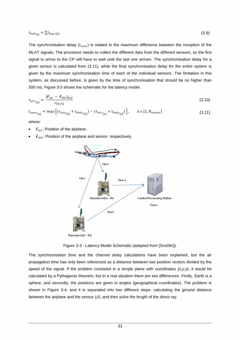
31
(3.9)
The synchronisation delay ( ) is related to the maximum difference between the reception of the
MLAT signals. The processor needs to collect the different data from the different sensors, so the first
signal to arrive to the CP will have to wait until the last one arrives. The synchronisation delay for a
given sensor is calculated from (3.11), while the final synchronisation delay for the entire system is
given by the maximum synchronisation time of each of the individual sensors. The limitation in this
system, as discussed before, is given by the time of synchronisation that should be no higher than
500 ms. Figure 3-3 shows the schematic for the latency model.
(3.10)
(3.11)
where:
: Position of the airplane.
: Position of the airplane and sensor, respectively.
Figure 3-3 - Latency Model Schematic (adapted from [Sns09c]).
The synchronisation time and the channel delay calculations have been explained, but the air
propagation time has only been referenced as a distance between two position vectors divided by the
speed of the signal. If the problem consisted in a simple plane with coordinates (x,y,z), it would be
calculated by a Pythagoras theorem, but in a real situation there are two differences. Firstly, Earth is a
sphere, and secondly, the positions are given in angles (geographical coordinates). The problem is
shown in Figure 3-4, and it is separated into two different steps: calculating the ground distance
between the airplane and the sensor ( ), and then solve the length of the direct ray.

32
Figure 3-4 - Air propagation distance.
The shortest path between two points, A and B, on a sphere is called the orthodrome. Given the
coordinates of each point the ground distance are known [Kui99]:
(3.12)
(3.13)
where:
: Latitude of the point A.
: Longitude of the point A.
: Latitude of the point B.
: Longitude of the point B.
: Earth effective radius in nautical miles.
: Angle between point A and B.
In order to calculate the length of the direct ray, three hypotheses have been tested: flat Earth (Figure
3-5), spherical Earth, and a simplification of the spherical Earth. The flat Earth model is the simplest,
and it is only valid for short distances in which the Earth curvature is negligible [Fig02]. Earth radius
should be taken into account for large distances, namely beyond the radio-horizon [Corr09].
Figure 3-5 - Flat Earth model.
(3.14)
where:
: Sensor‟s height.
: Airplane‟s altitude.
: Distance separating the airplane from the sensor.

33
The second hypothesis is the most accurate one, because it uses a theoretical model to account for
Earth radius. This model shows different results from the flat one, especially for large distances. The
schematic for the Earth model is also represented by Figure 3-4 and it solves the problem by
approximating the sphere to a flat model but with a correction of the sensor‟s and airplane‟s height,
called effective height. The height correction is related to the distance from the reflection point. The
equations necessary to correct the heights of the sensor and airplane are (3.15), (3.16), (3.17), (3.18)
and must be solved in that order [Fig02]. After that, (3.14) is used with both heights corrected.
It must be taken into consideration that this calculation is performed for each airplane position as
many times as the number of sensors in the network. Solving a third degree equation when multiple
points are being analysed may result in a high simulation delay.
(3.15)
(3.16)
(3.17)
(3.18)
where:
: Equivalent sensor‟s height in the flat Earth model.
: Equivalent airplane‟s height in the flat Earth model.
: Ground distance between the sensor and the reflection point.
: Ground distance between the airplane and the reflection point.
The third and last model is only valid for the WAM system, the simplification coming from the fact that
the altitude of the airplane is many times larger than the sensor‟s height, even considering sensors in
high hills. This fact implies that the point of specular reflection is in the nearby region of the sensor,
resulting in a very small compared with . Using this simplification, (3.19), the effective heights of
the airplane and sensor is given by (3.20) and (3.21).
(3.19)
(3.20)
(3.21)
Considering the three possible ways to calculate the length of the direct ray, the relative error of the
models comparing to the spherical Earth model is less than for the flat Earth, and less than
for the spherical Earth simplification, assuming:

34
It is reasonable to assume that any model can be used for a MLAT system, but the spherical Earth
model is not used because of the elapsed time solving the third degree equation. For the LAM
analysis, the flat Earth model is used, and for the WAM analysis, the spherical Earth simplified one is
used. The latter allows prevention of the increase in the coverage radius that is possible in other
MLAT systems.
This model is used to predict the difference between the times of arrival to the CP originated by the
messages sent from every sensor. It should be noticed that two effects are not being considered: the
deviation of the MLAT system processing time, and the extra delay by using more than one link. This
last effect can be for either using two different types of links or having more than one hop, and in both
cases there is a time elapsed for receiving the message and forwarding it to the next link.
This section gives the basic equations and foundation for the implementation of the latency simulator,
which calculates the expected delay for airplanes located in a given position.
3.3 Maximum Latency Model
NAV‟s Lisbon WAM system, which is already being implemented, will have all of the sensors outside
the airport, except one, with VPN links to connect them to the CP. It is essential to have an estimation
of the maximum tolerable delay that these links must support, in order to negotiate with the service
provider. The prediction of this latency is quite similar to the latency model, but in this case it considers
that the fastest sensor is one of the sensors located in the airport.
The latency between different RUs depends on the position of the airplane, but the maximum value of
the difference is given by the distance between both sensors, plus the difference in the link delay.
Figure 3-6 contains a schematic analysis to model the maximum distance between two sensors and
an airplane. In this case, it considers that one sensor is located in the airport and the other is any
WAM sensor. In Figure 3-6, is defined as the shortest path between the airplane and the WAM
sensor, the same distance but to the airport sensor, and the distance between both sensors. It is
easily seen that the alternative path to the sensor WAM ( ) is always larger than . By
analysing the worst case in Figure 3-6, the conclusion is that the maximum difference between and
is .
The equation describing the solution for the maximum delay in a VPN is:
(3.22)
where:
: Maximum delay for the rented VPN system for sensor i.
: Maximum synchronisation time allowed by the system.
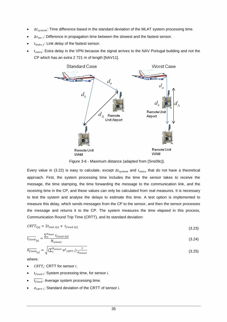
35
: Time difference based in the standard deviation of the MLAT system processing time.
: Difference in propagation time between the slowest and the fastest sensor.
: Link delay of the fastest sensor.
: Extra delay in the VPN because the signal arrives to the NAV Portugal building and not the
CP which has an extra 2 721 m of length [NAV11].
Figure 3-6 - Maximum distance (adapted from [Sns09c]).
Every value in (3.22) is easy to calculate, except and that do not have a theoretical
approach. First, the system processing time includes the time the sensor takes to receive the
message, the time stamping, the time forwarding the message to the communication link, and the
receiving time in the CP, and these values can only be calculated from real measures. It is necessary
to test the system and analyse the delays to estimate this time. A test option is implemented to
measure this delay, which sends messages from the CP to the sensor, and then the sensor processes
the message and returns it to the CP. The system measures the time elapsed in this process,
Communication Round Trip Time (CRTT), and its standard deviation:
(3.23)
(3.24)
(3.25)
where:
: CRTT for sensor .
: System processing time, for sensor .
: Average system processing time.
: Standard deviation of the CRTT of sensor .
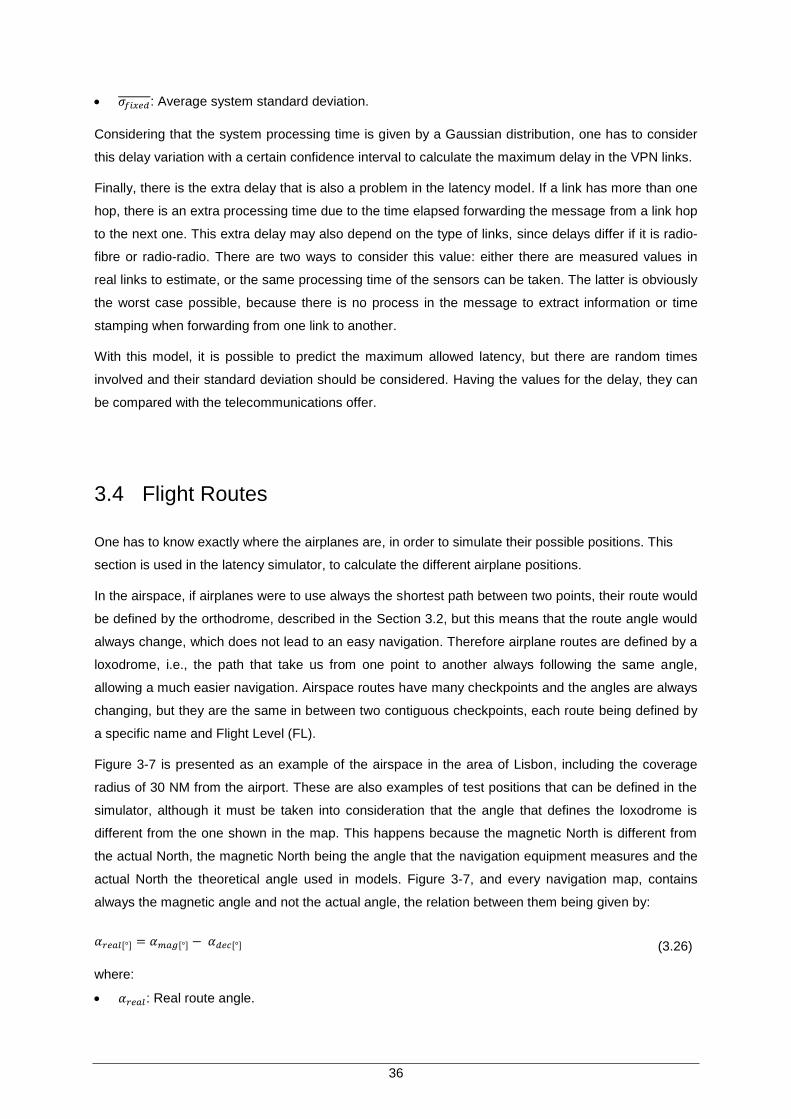
36
: Average system standard deviation.
Considering that the system processing time is given by a Gaussian distribution, one has to consider
this delay variation with a certain confidence interval to calculate the maximum delay in the VPN links.
Finally, there is the extra delay that is also a problem in the latency model. If a link has more than one
hop, there is an extra processing time due to the time elapsed forwarding the message from a link hop
to the next one. This extra delay may also depend on the type of links, since delays differ if it is radio-
fibre or radio-radio. There are two ways to consider this value: either there are measured values in
real links to estimate, or the same processing time of the sensors can be taken. The latter is obviously
the worst case possible, because there is no process in the message to extract information or time
stamping when forwarding from one link to another.
With this model, it is possible to predict the maximum allowed latency, but there are random times
involved and their standard deviation should be considered. Having the values for the delay, they can
be compared with the telecommunications offer.
3.4 Flight Routes
One has to know exactly where the airplanes are, in order to simulate their possible positions. This
section is used in the latency simulator, to calculate the different airplane positions.
In the airspace, if airplanes were to use always the shortest path between two points, their route would
be defined by the orthodrome, described in the Section 3.2, but this means that the route angle would
always change, which does not lead to an easy navigation. Therefore airplane routes are defined by a
loxodrome, i.e., the path that take us from one point to another always following the same angle,
allowing a much easier navigation. Airspace routes have many checkpoints and the angles are always
changing, but they are the same in between two contiguous checkpoints, each route being defined by
a specific name and Flight Level (FL).
Figure 3-7 is presented as an example of the airspace in the area of Lisbon, including the coverage
radius of 30 NM from the airport. These are also examples of test positions that can be defined in the
simulator, although it must be taken into consideration that the angle that defines the loxodrome is
different from the one shown in the map. This happens because the magnetic North is different from
the actual North, the magnetic North being the angle that the navigation equipment measures and the
actual North the theoretical angle used in models. Figure 3-7, and every navigation map, contains
always the magnetic angle and not the actual angle, the relation between them being given by:
(3.26)
where:
: Real route angle.
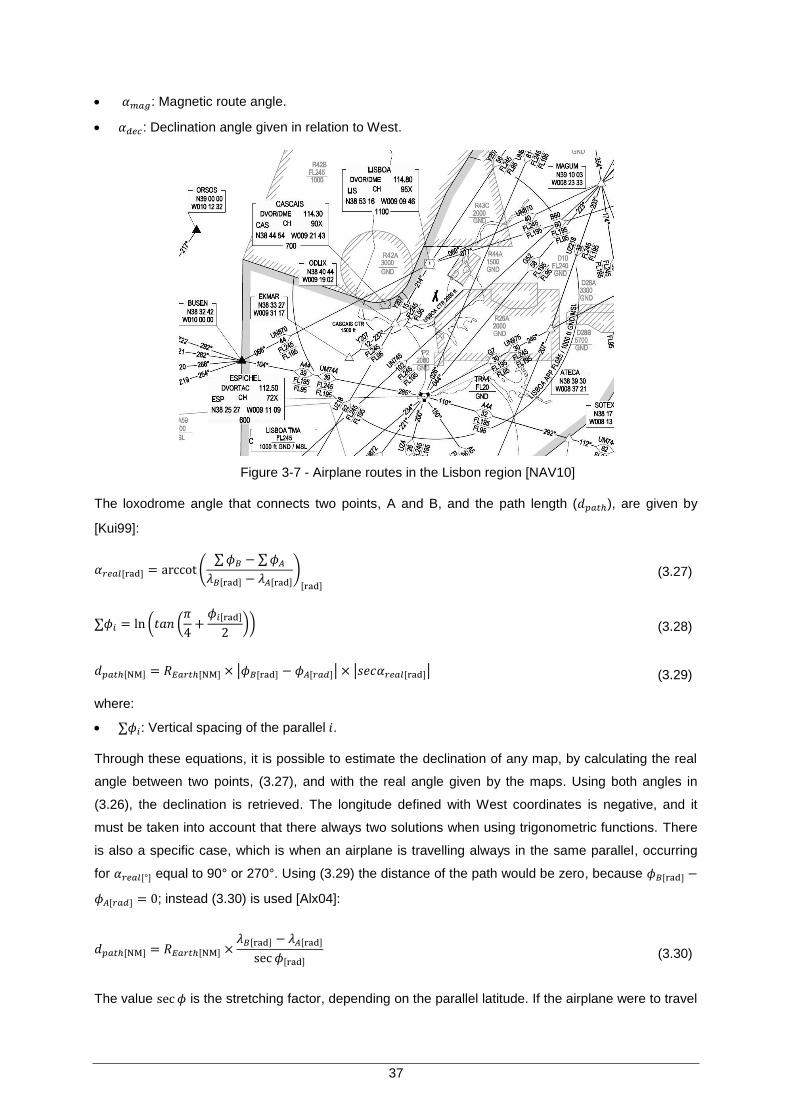
37
: Magnetic route angle.
: Declination angle given in relation to West.
Figure 3-7 - Airplane routes in the Lisbon region [NAV10]
The loxodrome angle that connects two points, A and B, and the path length ( ), are given by
[Kui99]:
(3.27)
(3.28)
(3.29)
where:
: Vertical spacing of the parallel .
Through these equations, it is possible to estimate the declination of any map, by calculating the real
angle between two points, (3.27), and with the real angle given by the maps. Using both angles in
(3.26), the declination is retrieved. The longitude defined with West coordinates is negative, and it
must be taken into account that there always two solutions when using trigonometric functions. There
is also a specific case, which is when an airplane is travelling always in the same parallel, occurring
for equal to 90° or 270°. Using (3.29) the distance of the path would be zero, because
; instead (3.30) is used [Alx04]:
(3.30)
The value is the stretching factor, depending on the parallel latitude. If the airplane were to travel

38
the equator, then this equation would be the equivalent to (3.30) with an angle of 0° or 180° [Alx04].
From the previous equations, one can also be concluded that a path can be defined from either a
starting position and an angle or two different positions. Two test possibilities are considered: a
section defined by two points, and a route defined by a starting point and a route angle. The difference
between them is that a section is always the path between both specified points at a certain altitude,
and the route calculates the intersection from the starting point with the desirable coverage radius.
With these two types of testing positions, it is possible to define every path of an airplane, being
limited to the coverage radius or not. It is complex to define a circle with latitude and longitude and
intersect it with a route; an easier approach is to travel through the route until the distance between
the point and the centre of the coverage area is approximately equal to the radius.
The last type of testing position is a particular case, approach to the runway, which is obviously very
used, but has different characteristics from the section or route. Details of the approach are described
in [NAV10], but it was decided [NAV11] that the approach should be defined by the runway orientation
angle, starting point of the approach, initial altitude, and descent angle in percentage. Figure 3-8
shows part of the approach definition for a runway in the Lisbon airport, containing the required
parameters (except the runway angle, which is included in [NAV10]). The approach distance and the
altitude are given by:
(3.31)
(3.32)
where:
: Initial Mean Sea Level (MSL) approach altitude.
: Airport MSL height.
: Descent angle.
: Height in a specific point of the approach.
: Relative distance from the starting point.
Unlike single points, every other test types have a certain number of points in the path they define, so
one must also include the number of test points for each path. The coordinates of the path separated
by a given interval are:
(3.33)
(3.34)
(3.35)
where:
: Distance between fixed intervals.
: Number of points to test in the path.

39
: Test position, if is the initial point and if is referring to the final point.
Figure 3-8 - Approach Lisbon RWY 03 [NAV10]
It should be noticed that the latitudes and longitudes may be positive or negative depending on the
airplane position: latitude is positive if the airplane is in the North hemisphere, and longitude is positive
when related to the East.
In summary, this Section contributes to the definition of the types of airplane positions that can be
used in the simulator, i.e., single points, sections, routes, and approaches.
3.5 Coverage model
In a MLAT system, every sensor has its own coverage map, being essential to know them, in order to
predict the required number of sensors in the whole system.
The first part of the coverage analysis is to get the land profile for each azimuth, which can be
achieved through Google servers, which are the basis for services like Google Maps or Google Earth.
An example of a land profile analysis retrieved from Google Earth is shown in Figure 3-9. Land
elevation values are given by the ground distance from the initial point, and if small distances are
considered this graph would be the only thing required to make the calculations; but, as explained in
latency model, flat Earth can only be applied for small distances. To calculate the coverage map, the
spherical Earth model is used, which assumes that the height of the ground sensor, airplane and land
obstacles are much smaller than the Earth radius.
Figure 3-9 - Google Earth elevation profile.

40
Firstly, one needs to calculate the specular reflection point, which in this particular case is not directly
related to the point in which there is the reflection, but to the radio horizon distance [Fig02].
(3.36)
where:
: Radio horizon distance of the specified position.
: Height in the specified position.
In Figure 3-10, the specific problem is described: every obstacle has a height correction, depending on
the distance from the tangent to the Earth surface, which is located at a distance of from the
sensor. Land elevations in the same reference plane are given by:
(3.37)
where:
: Distance from the sensor to the obstacle.
: Radio horizon distance for the sensor, using (3.36).
: Height of the obstacle.
Equation (3.37) considers that , meaning that any distance in the new reference plane is
approximately the same as in the Earth surface. From all elevations in the same reference plane,
dotted line in Figure 3-10, the coverage line is calculated.
For each obstacle, there is a coverage line with an angle, , the goal being to determine the final
coverage line angle, , that is given by the highest . Each angle depends on the distance from
the sensor and the obstacle‟s height. Sensor‟s height does not need to be considered, because its
equivalent height in the reference plane is always zero. The coverage angle is given by:
(3.38)
Figure 3-10 - Coverage diagram model.
Figure 3-10 illustrates two different airplane positions: position 1 and position i. The former is the case
in which there is no obstruction, hence, the coverage distance is given by the sum of the radio
horizons of the sensor plus the one of the airplane. For the latter, the coverage distance is given by
the intersection of the airplane with the coverage line, i.e.:

41
(3.39)
The effective height of the airplane is calculated in the same way as used for obstacles, (3.37), but it
also depends on the distance between airplane and sensor. Replacing (3.37) in (3.39) and simplifying:
(3.40)
The solution of (3.40) gives the cover distance for a given airplane‟s height and azimuth. All these
steps enable the calculation of coverage for a given azimuth, but the coverage of a sensor needs to be
radial, meaning that this calculation needs to be performed for many azimuths in [0°, 360°].
The sensors are limited to a maximum range and can even be limited by configuration, so this
parameter may be different for each sensor. After analyzing two reference suppliers of MLAT sensors,
Comsoft [Com11] and ERA [ERA10], the first has a maximum coverage of 250NM while the other has
200NM. From the market availability, the maximum possible range of the sensors is considered to be
around 200 NM. The parameter of the range must also be considered in the coverage analysis and
the maximum coverage cannot exceed this limitation of the equipment. After calculating , it must
be compared with the maximum allowed distance between the airplane and the sensor.
To calculate the maximum range for a given FL, two equations must be used, (3.37) and (3.41).
(3.41)
where:
: Maximum range of the sensor.
: Maximum covering distance on the ground for the specific flight level.
The intersection of the flight level with the coverage line results in a second degree equation, (3.40),
but for the maximum distance the solution is given by a fourth degree one. Due to this fact, and also
considering that these calculations are done only once for each sensor, an iterative process is used.
With the coverage distance and the maximum distance, for each azimuth, the final coverage is given
by the minimum of ( ).
All the procedures to analyse the coverage of a given sensor have been shown, but for a MLAT
system our interest is for many sensors, so a way of classifying each sensor is required. Two
comparisons have been developed for the individual coverage in the required area: qualitative and
quantitative. Maps are divided into the covered districts and the Terminal Manoeuvring Area (TMA),
the latter region being included because it requires a special attention due to particular requirements.
Starting by the qualitative analysis, it is useful to know which area inside the district is really covered,
as well as a notion of the quantity covered. Table 3-4 contains the legend to be used when classifying
each of the districts, four main categories being considered: total, almost total (total -), half and
nothing (0). The category Total-NE and Half S are only shown as example and it must be noticed that
any other combination of geographical directions are valid in conjugation with the word Total- or Half.
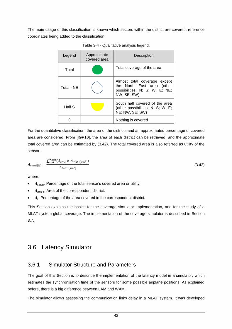
42
The main usage of this classification is known which sectors within the district are covered, reference
coordinates being added to the classification.
Table 3-4 - Qualitative analysis legend.
Legend Approximate covered area
Description
Total
Total coverage of the area
Total - NE
Almost total coverage except the North East area (other possibilities; N; S; W; E; NE; NW, SE; SW)
Half S
South half covered of the area (other possibilities; N; S; W; E; NE; NW, SE; SW)
0 Nothing is covered
For the quantitative classification, the area of the districts and an approximated percentage of covered
area are considered. From [IGP10], the area of each district can be retrieved, and the approximate
total covered area can be estimated by (3.42). The total covered area is also referred as utility of the
sensor.
(3.42)
where:
: Percentage of the total sensor‟s covered area or utility.
: Area of the correspondent district.
: Percentage of the area covered in the correspondent district.
This Section explains the basics for the coverage simulator implementation, and for the study of a
MLAT system global coverage. The implementation of the coverage simulator is described in Section
3.7.
3.6 Latency Simulator
3.6.1 Simulator Structure and Parameters
The goal of this Section is to describe the implementation of the latency model in a simulator, which
estimates the synchronisation time of the sensors for some possible airplane positions. As explained
before, there is a big difference between LAM and WAM.
The simulator allows assessing the communication links delay in a MLAT system. It was developed

43
considering the systems already implemented, but it was developed to be as compatible as possible to
any other MLAT system. In order to accomplish this, it supports the most used types of communication
links in MLAT, and the possibility of the existence of more than one type of link for each sensor.
The simulator is described in
Figure 3-11, and it has been implemented using MatlabR2007b [MatL11]. First the system and the
airplane test positions are described, and then the latency model from Section 3.2 is applied.
Afterwards, there is a result analysis to determine the synchronisation time and also which messages
arrive within the maximum time allowed. Finally, the output is generated with the results of the system
analysis for each position that was tested. Although there are differences between LAM and WAM, the
general structure of the simulator is the same, differing only in some specific algorithms.
System
description
Test Positions
(section 3.4)
Latency model
(section 3.2)Result analysis Write output
Figure 3-11- Simulator general structure.
The simulator requires two input files that are selected using the Graphical User Interface (GUI) and a
few parameters also introduced in the GUI:
(System description file).xlsx: it contains the description of the MLAT system with every sensor
and the communication links.
(Test positions file).xlsx: it contains the positions of the airplanes to be tested (Section 3.4).
Both files differ if the simulation is for a LAM or WAM system, and a more details can be found in
Annex A, which contains the user manual of the simulator. In the GUI, although default values are
defined, it is possible to change the following parameters:
Maximum synchronisation time.
Coverage radius.
Declination in the area to analyse.
Coverage radius and declination are only used in the WAM analysis, and the radius is defined taking
the coordinates defined by the CPS of the system description file.
The output is written in an Excel file (*.xlsx) containing, for each test position, the results of the latency
model, its name being the concatenation of “Output_” with the name of the test positions file.
3.6.2 LAM and WAM Simulator
The LAM flowchart is required to understand its algorithm. Although this is just the implementation of
the latency model, more computations are required, Figure B.1.
The LAM simulator starts by reading the first input file that contains every sensor on the network, and
the links each one has. With this information, the link delay ( ) of each sensor is calculated, which
depends on the communication link, explained in the Section 3.2.

44
The second step is to read and analyse the second input file, which contains the test positions. For
each point, the simulator reads the coverage, also included in the second input file, and calculates the
propagation delay from the position to each of the covering sensors ( ); this propagation delay is
then summed to the link delay previously calculated. Only the fastest five sensors are considered to
calculate the synchronisation; more sensors could be used, but to meet the requirements only five are
considered critical. This synchronisation time is the difference between the fastest and slowest of the
five sensors.
The output format of the LAM analysis is different from the WAM one, because the latter has much
more information to display, which is not considered to show the delay of each position to each
sensor, unlike LAM. The output file states, for each position, the synchronisation time, the fastest and
the fifth fastest (slowest) sensor, and the total delay for each sensor that covers that position.
The other type of analysis performed by the simulator is the WAM system. The WAM flowchart is
presented in Figure B.2, and also describes the steps of the simulator.
Besides the format difference between both input files, the first part that involves reading the
description file and test positions is the same as in the LAM algorithm. The main difference comes
when the types of path are identified. For the single point test position, the analysis is similar, but for
sections, approach, and routes, there are a few calculations to perform before having the final test
points to test.
For the section, as explained in Section 3.4, the simulator calculates all points in it based on the total
number of points to test. The approach is identified by a starting position and an angle, the landing
position is calculated, and with these two coordinates a section is defined; the same function used in
the section calculation to get the intermediate points is used. Besides the intermediate points, the flight
altitude for each point also needs to be computed. Finally, for the route, it intersects the coverage area
by an iterative process, and there are two situations to define the two points for the route:
Initial point inside the coverage area: it only calculates one intersection with the coverage area,
and the other point to define the section is the starting position.
Initial point outside the coverage area: the two points used to define the section are intersections
with the coverage area.
Discovering the two points that define the route, the simulator‟s procedure is similar to the section test,
computing the intermediate points by using the section method. When there is no more analysis to
perform, the simulator writes an excel output file discriminating every test positions types, the
intermediate positions, and the delay analysis. An extra output in a WAM analysis is the list of sensors
that are able to forward the message to the CP within the synchronisation time.
This Section roughly describes the simulator. In terms of how to use the simulator, there is a more
detailed explanation in Annex A.
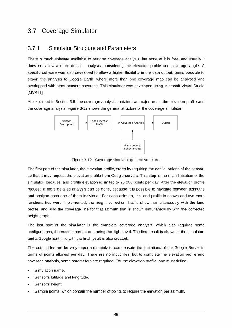
45
3.7 Coverage Simulator
3.7.1 Simulator Structure and Parameters
There is much software available to perform coverage analysis, but none of it is free, and usually it
does not allow a more detailed analysis, considering the elevation profile and coverage angle. A
specific software was also developed to allow a higher flexibility in the data output, being possible to
export the analysis to Google Earth, where more than one coverage map can be analysed and
overlapped with other sensors coverage. This simulator was developed using Microsoft Visual Studio
[MVS11].
As explained in Section 3.5, the coverage analysis contains two major areas: the elevation profile and
the coverage analysis. Figure 3-12 shows the general structure of the coverage simulator.
Sensor
Description
Land Elevation
ProfileCoverage Analysis Output
Flight Level &
Sensor Range
Figure 3-12 - Coverage simulator general structure.
The first part of the simulator, the elevation profile, starts by requiring the configurations of the sensor,
so that it may request the elevation profile from Google servers. This step is the main limitation of the
simulator, because land profile elevation is limited to 25 000 points per day. After the elevation profile
request, a more detailed analysis can be done, because it is possible to navigate between azimuths
and analyse each one of them individual. For each azimuth, the land profile is shown and two more
functionalities were implemented, the height correction that is shown simultaneously with the land
profile, and also the coverage line for that azimuth that is shown simultaneously with the corrected
height graph.
The last part of the simulator is the complete coverage analysis, which also requires some
configurations, the most important one being the flight level. The final result is shown in the simulator,
and a Google Earth file with the final result is also created.
The output files are be very important mainly to compensate the limitations of the Google Server in
terms of points allowed per day. There are no input files, but to complete the elevation profile and
coverage analysis, some parameters are required. For the elevation profile, one must define:
Simulation name.
Sensor‟s latitude and longitude.
Sensor‟s height.
Sample points, which contain the number of points to require the elevation per azimuth.

46
Range to cover, which contains the range to get the elevation profile.
Number of azimuths, which contains the number of azimuths to get the elevation profile in the
defined range.
To complete the coverage analysis, three more parameters are required:
Flight level of the airplane.
Maximum range of the sensor.
Colour to display the output in Google Earth.
Besides the configuration parameters, there are three types of output files. The first output file is to
save the data collected from Google servers, and elevation profile parameters, the second is to
generate the final coverage map in Google Earth, and the third is an auxiliary file that can save any
graph from the application to an image file.
The first output file allows saving the land profile of a certain sensor, only later making the coverage
analysis for one or more flight levels. With this functionality, it is possible to minimise servers‟
limitations, because data can be collected in different days or with different IP addresses, and only
after having all data, one can study the global coverage. The format of this output file is *.txt whose
name is the concatenation of “Output_” with the simulation name. The file contains all parameters:
simulation name, latitude, longitude, sensor height, number of azimuths and for each azimuth contains
the number of points, the azimuth degree, and each of the points. Each point contains the elevation,
the coordinates, and the distance from the sensor‟s location.
The second output file is a Google Earth one with the final coverage map. The format *.kml is a type of
xml file that Google uses to represent markers, lines or polygons [Go11a]. Knowing the covered
distance for each azimuth, they are translated into latitude and longitude, and after having all
azimuths, the *.kml polygon is created. The colour of the polygon is a parameter defined in the
configuration, and the file name is the name of the simulation.
The final output file is to retrieve simulator images, instead of using a print screen solution. It may be
saved with most of the common image file types, and the name is defined by the user. This file is not
very important for the simulator results, and it is only used to retrieve a more specific analysis for a
certain azimuth.
This Section summarises the possible outputs of the simulator, which are used to analyse the results.
A brief summary of the structure and functionalities of the coverage simulator is also made.
3.7.2 Elevation Profile
With the definition of the elevation profile parameters defined in Section 3.7.1, it is possible to
complete the request of the elevation profile, which is the beginning of the coverage analysis study.
Google developed two request possibilities to get elevation profiles: one is by giving a single point and
the other by giving a path with the desired number of points in between. Both possibilities can be
used, but the simplest one, used in the simulator, is the latter. The requests to Google are based on

47
URL requests, and there is a library that basically builds the HTTP messages and receives the
response obtained from Google [Go11c].
It has already been explained that this service has a few limitation [Go11b]: 2 500 requests per day,
512 elevation points per request, and 25 000 points per day. The limitation of 2 500 requests per day
means that even if the possibility of requesting individually each point had been considered, it could
not be used, because 2 500 points would be the maximum to request. The simulator does not control
the number of points that were actually requested, even though it informs the user if the request was
successful or not. It must be taken into account that the number of requested points is given by:
(3.43)
where:
: Total number of points requested to Google in the simulation.
: Number of azimuths to get the elevation profile.
: Number of elevation samples per azimuth.
Another way of improving efficiency, concerning Google limitations, is to make the coverage analysis
just for a limited range. For instance, if a sensor has a sector covering the ocean, this area may be
excluded from the analysis and one only performs an 180o analysis.
The finalisation of the elevation profile requests consist of defining the paths for which the request is
going to be made. The azimuths to analyse are given by (3.44), and the coordinates of the path from a
sensor location to another following the azimuth previously defined, (3.34) and (3.35). These
equations also need to define the distance for which the elevation profile must be retrieved, and for
this matter a range of 80 NM is considered. At first, some results were taken for 100 NM, but
considering that every point defining the coverage line is within 80 NM, the distance was reduced,
improving the accuracy of the elevation profile. This range to ask for the elevation profile is different
from the coverage range, because the obstacles very far away from the sensor will not influence the
coverage angle.
(3.44)
where:
: Angle of the respective azimuth.
: Minimum of the range defined by the user.
: Amplitude of the range defined by the user.
: Actual azimuth .
After data are collected, their export is done, saving the first output file. The procedure to get the
complete elevation profile has been described, but the data analysis is still missing. The elevation
profile of the first azimuth is displayed, but it is possible to travel through every other azimuth. These
graphs do not require any more calculations, besides the values retrieved from Google. The result of a

48
land profile example is shown in Figure C.4.
The second step of the elevation profile is to correct the heights using (3.37), an example of the height
correction for the same example used in Figure C.4 being shown in Figure C.5. The effective land
height is displayed together with the land profile elevation. From (3.37), it is concluded that the higher
the distance from the obstacle to the sensor‟s radio horizon, the larger the height correction. This
specific sensor is located at approximately 800 m MSL from the ground, which, from (3.36), gives a
radio horizon of 101 km. Beyond the radio horizon, the increase in the height correction is not linear
but squared.
3.7.3 Coverage
There are basically two types of coverage that are distinguished in the simulator: coverage profile and
global coverage. The former calculates individually the coverage line for each azimuth, and plots it in
the simulator, while the latter calculates the global coverage and plots the coverage map.
The coverage profile flowchart is shown in Figure 3-13. An azimuth land profile must be selected to
calculate a coverage line, and then land profile heights are corrected. With the corrected heights, the
simulator calculates every coverage line for each of the elevation points retrieved from Google
servers, always registering the maximum angle, (3.38). Finally, after computing every coverage line,
the simulator plots the result.
Beginning
Load Azimuth
land profile
Correct Height
of Profile
Number
points > 0
Calculate
Coverage LineTrue
Display
Coverage Line
With Maximum
Angle
Update
Maximum
Angle
False
Finish
Number of
Points -1
Figure 3-13 - Coverage line flowchart.
Figure C.6 contains the coverage line calculated for the sensor‟s azimuth used in the example of
Section 3.7.2. It is displayed over the effective height profile, and the influence of the obstacles in the
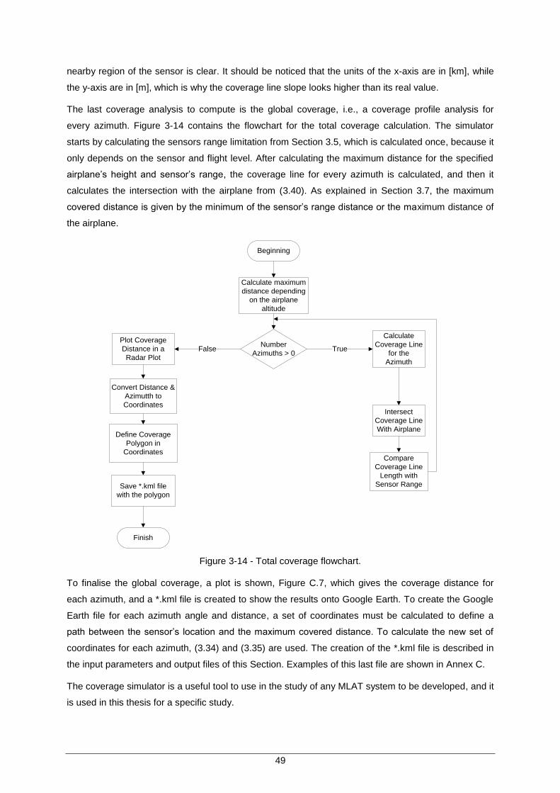
49
nearby region of the sensor is clear. It should be noticed that the units of the x-axis are in [km], while
the y-axis are in [m], which is why the coverage line slope looks higher than its real value.
The last coverage analysis to compute is the global coverage, i.e., a coverage profile analysis for
every azimuth. Figure 3-14 contains the flowchart for the total coverage calculation. The simulator
starts by calculating the sensors range limitation from Section 3.5, which is calculated once, because it
only depends on the sensor and flight level. After calculating the maximum distance for the specified
airplane‟s height and sensor‟s range, the coverage line for every azimuth is calculated, and then it
calculates the intersection with the airplane from (3.40). As explained in Section 3.7, the maximum
covered distance is given by the minimum of the sensor‟s range distance or the maximum distance of
the airplane.
Beginning
Finish
Number
Azimuths > 0
Plot Coverage
Distance in a
Radar Plot
False
Calculate
Coverage Line
for the
Azimuth
True
Intersect
Coverage Line
With Airplane
Convert Distance &
Azimutth to
Coordinates
Define Coverage
Polygon in
Coordinates
Save *.kml file
with the polygon
Compare
Coverage Line
Length with
Sensor Range
Calculate maximum
distance depending
on the airplane
altitude
Figure 3-14 - Total coverage flowchart.
To finalise the global coverage, a plot is shown, Figure C.7, which gives the coverage distance for
each azimuth, and a *.kml file is created to show the results onto Google Earth. To create the Google
Earth file for each azimuth angle and distance, a set of coordinates must be calculated to define a
path between the sensor‟s location and the maximum covered distance. To calculate the new set of
coordinates for each azimuth, (3.34) and (3.35) are used. The creation of the *.kml file is described in
the input parameters and output files of this Section. Examples of this last file are shown in Annex C.
The coverage simulator is a useful tool to use in the study of any MLAT system to be developed, and it
is used in this thesis for a specific study.

50
3.7.4 Simulator Assessment
The values of the simulator must be compared with a real coverage simulator available, in order to
assess it. In this thesis, some coverage maps are shown and they can be used to compare with the
simulator results.
Choosing the WAM Fanhões sensor, the comparison between both simulators is shown in Figure
3-15. Both analyses calculate the LoS coverage.
The parameters used in the coverage simulator were 36 azimuths and 500 elevation points per
azimuth. With 36 azimuths, it is expected that the accuracy decreases comparing with NAV‟s software,
but this simulator is always limited to a few number of azimuths, due to the Google server limitation on
elevation requests. Besides the clear difference in accuracy, due to the previously mentioned
limitations, there is a reduction in the length of each azimuth. For instance, the south of Algarve is
considered to be covered in NAV‟s software, where as in the coverage simulator it is not completely
covered.
Even though having these two limitations, and assuming that the software not developed in this thesis
is precise, the coverage shape is very similar. Having a shorter range means that this simulator is
more restrictive than the other, otherwise the implications would be worse. With a higher coverage
range the validity of the results near the cell edges would be arguable.
a) Fanhões with NAV‟s software b) Fanhões with coverage simulator
Figure 3-15 - Coverage simulator assessment.
Another test for the simulator concerns the sensor range limiting coverage. In order to test the range
limitation to 200 NM, which is the value considered for the study, the same sensor was used, but the
FL was increased to FL300, so that the coverage exceeds the sensor‟s maximum range, Figure 3-16.
For this specific case, the radio horizon of the airplane plus sensor is 220.4 NM, but the range limits
that distance to 199.8 NM.

51
Figure 3-16 - Coverage for FL300 and maximum range 200 NM.
This Section validated the developed coverage simulator, so that it may be used as a tool to design
MLAT systems. More information concerning the use of the simulator can be found in Annex C, where
the user‟s manual.


53
Chapter 4
Results and Data Analysis
4 Results and Data Analysis
In this chapter, the simulation results for the analysis of the current multilateration systems, the
complete preliminary study for a new multilateration system, and tolerable delay for the VPN links in
Lisbon are analysed. Other small analysis to the multilateration systems are analysed, such as the
communication link capacity and the impact of the regulator requirements in the systems.

54
4.1 NAV Portugal Implemented Systems
Currently, there is one operational MLAT system, one being finalised and another in procurement
phase. Although there are studies being conducted for other MLAT systems, only the three described
have the study finalised.
The first MLAT system is located in the Lisbon airport: it consists of a system on the airport grounds
(LAM), and is already in operational use. There is a project (in procurement phase) to expand this
system to cover a 30 NM radius from the Airport (WAM) that foreseen to be concluded during the next
year [NAV11]. Although there are differences between a LAM and WAM, concerning this thesis, both
types are described by the sensors location, the communication link description of each sensor, and
the individual coverage analysis. The final system to be analysed is located in the Azores.
The Lisbon LAM system is composed of the CPS, fourteen RUs and two reftrans. In Figure 4-1, the
sensors are identified by 1 to 14 and the blue squares represent the reftrans, x1 and x2.
Figure 4-1 - Lisbon LAM system sensors location first phase (extracted from [Sns09c]).
The individual and global coverage of the sensors is shown in Annex D, Figure D.1 to Figure D.4. The
coverage maps are used when analysing the effects of the delay in the system, and also to give a
perspective of the study that needs to be conducted prior to the decision concerning the sensors
location.
Table 4-1 describes, in a more detailed way, the RUs geographical coordinates, above ground level
(AGL), communication link used, their length and capacity. Column ID in Table 4-1 is the name
identification of the corresponding component, which is used in what follows. All RUs, except RU7 that
is co-located with the CPS, use a fibre link with lengths smaller than 6 km and with a capacity of
100Mbps. Reftrans, which are co-located with sensors RU1 and RU7, do not have a specified
communication link, because the synchronisation is via radio link, the only requirements being that
every RU have LoS for at least one reftran.
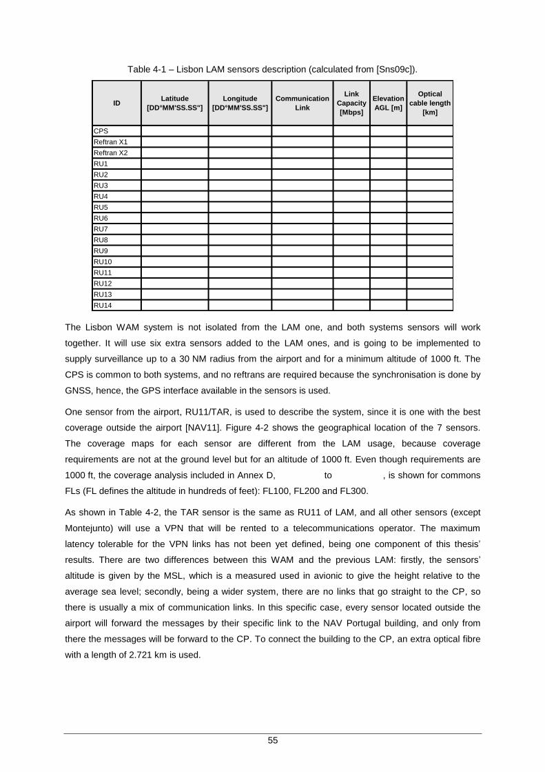
55
Table 4-1 – Lisbon LAM sensors description (calculated from [Sns09c]).
IDLatitude
[DD°MM'SS.SS"]
Longitude
[DD°MM'SS.SS"]
Communication
Link
Link
Capacity
[Mbps]
Elevation
AGL [m]
Optical
cable length
[km]
CPS
Reftran X1
Reftran X2
RU1
RU2
RU3
RU4
RU5
RU6
RU7
RU8
RU9
RU10
RU11
RU12
RU13
RU14
The Lisbon WAM system is not isolated from the LAM one, and both systems sensors will work
together. It will use six extra sensors added to the LAM ones, and is going to be implemented to
supply surveillance up to a 30 NM radius from the airport and for a minimum altitude of 1000 ft. The
CPS is common to both systems, and no reftrans are required because the synchronisation is done by
GNSS, hence, the GPS interface available in the sensors is used.
One sensor from the airport, RU11/TAR, is used to describe the system, since it is one with the best
coverage outside the airport [NAV11]. Figure 4-2 shows the geographical location of the 7 sensors.
The coverage maps for each sensor are different from the LAM usage, because coverage
requirements are not at the ground level but for an altitude of 1000 ft. Even though requirements are
1000 ft, the coverage analysis included in Annex D, Figure D.5 to Figure D.11, is shown for commons
FLs (FL defines the altitude in hundreds of feet): FL100, FL200 and FL300.
As shown in Table 4-2, the TAR sensor is the same as RU11 of LAM, and all other sensors (except
Montejunto) will use a VPN that will be rented to a telecommunications operator. The maximum
latency tolerable for the VPN links has not been yet defined, being one component of this thesis‟
results. There are two differences between this WAM and the previous LAM: firstly, the sensors‟
altitude is given by the MSL, which is a measured used in avionic to give the height relative to the
average sea level; secondly, being a wider system, there are no links that go straight to the CP, so
there is usually a mix of communication links. In this specific case, every sensor located outside the
airport will forward the messages by their specific link to the NAV Portugal building, and only from
there the messages will be forward to the CP. To connect the building to the CP, an extra optical fibre
with a length of 2.721 km is used.

56
Figure 4-2 - Lisbon WAM sensors location (using Google Earth).
Table 4-2 - WAM sensors description (calculated from [NAV11])
RU IDLatitude
[DD°MM'SS.SS"]
Longitude
[DD°MM'SS.SS"]
Elevation
MSL [m]
Communication
Type
Communication
link Capacity
[Mbps]
Communication
link length [km]
extra optical
fibre length
[km]
Arrabida 38°29'34"N 8°57'44"W 356 VPN 0.2 N/A 2.72
Caparica 38°38'32"N 9°13'17"W 95 VPN 0.2 N/A 2.72
Espichel 38°25'27"N 9°11'09"W 183 VPN 0.2 N/A 2.72
Fanhões 38°53'16"N 9°09'46"W 340 VPN 0.2 N/A 2.72
Montargil 39°04'38"N 8°11'15"W 235 VPN 0.2 N/A 2.72
MonteJunto 39°10'23"N 9°02'52"W 670 Microwave link 6.0 47.72 2.72
TAR (RU 11)
airport38°45'50"N 9°08'20"W 135 Fibre 100.0 3.47 N/A
Concerning the located in the Azores, all communications use microwave links, and connect every
sensor to the CPS located in the airport of Horta, more specifically in the airport control Tower (TWR).
Figure 4-3 contains the sensors location in Google Earth and the microwave links represented as red
lines. TWR Horta, represented by an airplane in Figure 4-3, is the CPS for this system. There are only
two sensors directly connected to the CP, GS_01 and GS_02, the rest being connected to GS_00 by
one or more microwave links, and from there they are connected to the CP using a repeater, triangle
in Figure 4-3 [ERA11]. A more detailed description of each sensor‟s location, link capacity and length,
number of hops per link is shown in Table 4-3.
The ground sensors have three possible configurations that can be used simultaneously: receiver,
transmitter and reftran. All sensors represented in Table 4-3 have receiving capabilities, but only
GS_00, GS_04, GS_05 and GS_07 can work as transmitters. The synchronisation of the sensors in
this system is similar to the one used in Lisbon‟s LAM, the sensors that incorporate the reftran
functionality being GS_00, GS_05 and GS_09.
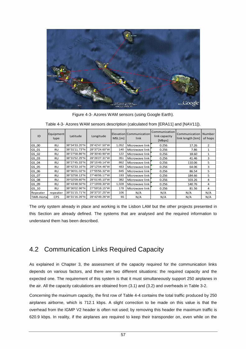
57
Figure 4-3- Azores WAM sensors (using Google Earth).
Table 4-3- Azores WAM sensors description (calculated from [ERA11] and [NAV11]).
IDEquipment
typeLatitude Longitude
Elevation
MSL [m]
Communication
link
Communication
link capacity
[Mbps]
Communication
link length [km]
Number
of hops
GS_00 RU 38°34'33.20"N 28°42'47.50"W 1,052 Microwave link 0.256 17.26 2
GS_01 RU 38°31'11.73"N 28°37'24.60"W 140 Microwave link 0.256 7.86 1
GS_02 RU 38°27'58.86"N 28°30'40.90"W 122 Microwave link 0.256 18.60 1
GS_03 RU 38°31'52.25"N 28°26'27.31"W 351 Microwave link 0.256 41.46 3
GS_04 RU 38°27'45.33"N 28°15'49.14"W 862 Microwave link 0.256 110.06 5
GS_05 RU 38°42'33.16"N 28°12'04.46"W 483 Microwave link 0.256 64.06 3
GS_06 RU 38°36'01.02"N 27°55'56.32"W 845 Microwave link 0.256 86.54 5
GS_07 RU 38°32'58.13"N 27°46'06.17"W 193 Microwave link 0.256 184.66 5
GS_08 RU 39°02'09.60"N 28°01'45.10"W 382 Microwave link 0.256 103.26 4
GS_09 RU 38°43'48.50"N 27°19'09.30"W 1,028 Microwave link 0.256 140.76 4
GS_10 RU 38°36'02.96"N 27°59'18.15"W 178 Microwave link 0.256 81.56 4
Repeater repeater 38°31'15.71"N 28°37'37.25"W 106 N/A N/A N/A N/A
TWR-Horta CPS 38°31'16.26"N 28°42'49.26"W 65 N/A N/A N/A N/A
The only system already in place and working is the Lisbon LAM but the other projects presented in
this Section are already defined. The systems that are analysed and the required information to
understand them has been described.
4.2 Communication Links Required Capacity
As explained in Chapter 3, the assessment of the capacity required for the communication links
depends on various factors, and there are two different situations: the required capacity and the
expected one. The requirement of this system is that it must simultaneously support 250 airplanes in
the air. All the capacity calculations are obtained from (3.1) and (3.2) and overheads in Table 3-2.
Concerning the maximum capacity, the first row of Table 4-4 contains the total traffic produced by 250
airplanes airborne, which is 712.1 kbps. A slight correction to be made on this value is that the
overhead from the IGMP V2 header is often not used; by removing this header the maximum traffic is
620.9 kbps. In reality, if the airplanes are required to keep their transponder on, even while on the

58
ground, the probability of having 250 airplanes airborne is even lower. Even so, for a critical
surveillance system this last requirement must be always guaranteed.
The calculation of the expected traffic in each communication link has been done for some possible
system configurations, meaning the different ratios of stationary, moving or airborne airplanes. A
useful characteristic of the requirements is that a moving airplane sends the same messages as a
moving vehicle, so the ratio of moving airplanes ( ) contains both vehicles and airplanes. Four
cases for the positions distribution were considered, all of them with a total of 250 targets, Table 4-4.
Table 4-4 - Results for different airplane positions.
Traffic without
overhead
Traffic with
overhead
00 00 100 142.1 712.1
50 25 025 078.4 383.4
70 15 015 Not calculated 274.7
80 10 010 Not calculated 220.4
This table illustrates the impact of the overhead in the messages, which itself is responsible by around
77 % of the exchanged volume, and also the influence of the number of airborne airplanes. In a real
situation, the possibility of having simultaneously 250 airplanes in the air is not realistic, and the most
realistic situation is closer to the 70/15/15 configuration. This difference means that the real expected
traffic is much smaller than the required capacity, and considering the difference from the 70/15/15
configuration to every airplane airborne, the capacity decreases around 61%.
Due to some factors, such as multipath, overlap of different signals (garbling) and interfering signals
(jamming), the receiving probability is reduced and as a consequence so does the required capacity.
Garbling is a problem that occurs from the different signals overlapping, being similar to multipath,
because both cause a distortion of the signal at reception, but garbling increases with the number of
airplanes, unlike multipath that only depends on the environment. Even if distorted, the receiving
signals may be used for identification, but they do not produce an accurate solution for the TDOA
algorithm, so they may be discarded, which obviously reduces the traffic in the communication link, but
leads also to a decrease in the detection probability [Nev05]. Interference is also an existing problem
to consider, having the same effect of signals corruption, thus, the messages are also discarded.
There is one last factor that could have implications in the reduction of the capacity required for the
communication links, i.e., coverage. If a sensor only covers a part of the surveillance area, it would be
also reasonable that instead of the 250 airplanes it would only cover a part of it. This occurs for a LAM
system, where the coverage maps in Annex D show that there is no sensor covering the entire airport.
On the other hand, the WAM systems coverage is much different. Even though requirements demand
a 1000 ft coverage, in a real situation airplanes fly above 9 500 ft, and most of them in the highest
routes around 29 500 ft. The coverage maps for the Lisbon WAM, Annex D, show that the coverage
area is much larger than the 30 NM radius from the airport, which means that no reduction in the traffic
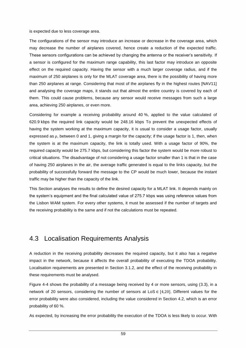
59
is expected due to less coverage area.
The configurations of the sensor may introduce an increase or decrease in the coverage area, which
may decrease the number of airplanes covered, hence create a reduction of the expected traffic.
These sensors configurations can be achieved by changing the antenna or the receiver‟s sensitivity. If
a sensor is configured for the maximum range capability, this last factor may introduce an opposite
effect on the required capacity. Having the sensor with a much larger coverage radius, and if the
maximum of 250 airplanes is only for the MLAT coverage area, there is the possibility of having more
than 250 airplanes at range. Considering that most of the airplanes fly in the highest routes [NAV11]
and analysing the coverage maps, it stands out that almost the entire country is covered by each of
them. This could cause problems, because any sensor would receive messages from such a large
area, achieving 250 airplanes, or even more.
Considering for example a receiving probability around 40 %, applied to the value calculated of
620.9 kbps the required link capacity would be 248.16 kbps To prevent the unexpected effects of
having the system working at the maximum capacity, it is usual to consider a usage factor, usually
expressed as , between 0 and 1, giving a margin for the capacity; if the usage factor is 1, then, when
the system is at the maximum capacity, the link is totally used. With a usage factor of 90%, the
required capacity would be 275.7 kbps, but considering this factor the system would be more robust to
critical situations. The disadvantage of not considering a usage factor smaller than 1 is that in the case
of having 250 airplanes in the air, the average traffic generated is equal to the links capacity, but the
probability of successfully forward the message to the CP would be much lower, because the instant
traffic may be higher than the capacity of the link.
This Section analyses the results to define the desired capacity for a MLAT link. It depends mainly on
the system‟s equipment and the final calculated value of 275.7 kbps was using reference values from
the Lisbon WAM system. For every other systems, it must be assessed if the number of targets and
the receiving probability is the same and if not the calculations must be repeated.
4.3 Localisation Requirements Analysis
A reduction in the receiving probability decreases the required capacity, but it also has a negative
impact in the network, because it affects the overall probability of executing the TDOA probability.
Localisation requirements are presented in Section 3.1.2, and the effect of the receiving probability in
these requirements must be analysed.
Figure 4-4 shows the probability of a message being received by 4 or more sensors, using (3.3), in a
network of 20 sensors, considering the number of sensors at LoS . Different values for the
error probability were also considered, including the value considered in Section 4.2, which is an error
probability of 60 %.
As expected, by increasing the error probability the execution of the TDOA is less likely to occur. With
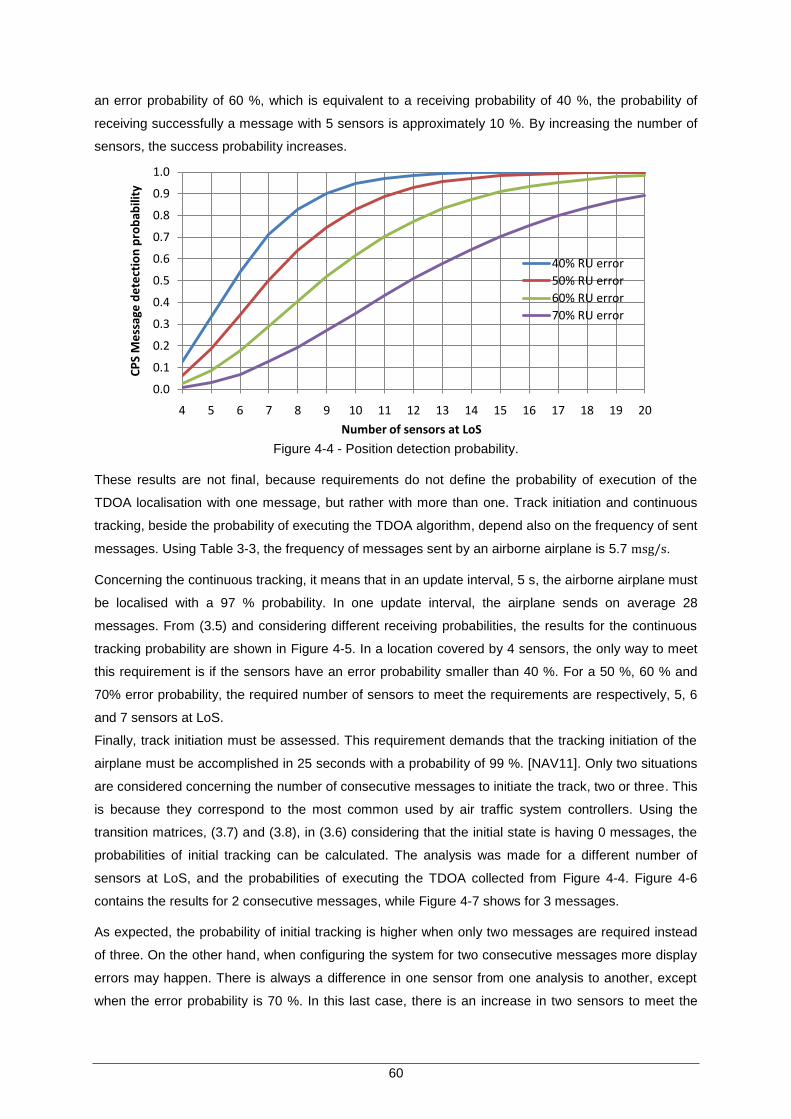
60
an error probability of 60 %, which is equivalent to a receiving probability of 40 %, the probability of
receiving successfully a message with 5 sensors is approximately 10 %. By increasing the number of
sensors, the success probability increases.
Figure 4-4 - Position detection probability.
These results are not final, because requirements do not define the probability of execution of the
TDOA localisation with one message, but rather with more than one. Track initiation and continuous
tracking, beside the probability of executing the TDOA algorithm, depend also on the frequency of sent
messages. Using Table 3-3, the frequency of messages sent by an airborne airplane is 5.7 .
Concerning the continuous tracking, it means that in an update interval, 5 s, the airborne airplane must
be localised with a 97 % probability. In one update interval, the airplane sends on average 28
messages. From (3.5) and considering different receiving probabilities, the results for the continuous
tracking probability are shown in Figure 4-5. In a location covered by 4 sensors, the only way to meet
this requirement is if the sensors have an error probability smaller than 40 %. For a 50 %, 60 % and
70% error probability, the required number of sensors to meet the requirements are respectively, 5, 6
and 7 sensors at LoS.
Finally, track initiation must be assessed. This requirement demands that the tracking initiation of the
airplane must be accomplished in 25 seconds with a probability of 99 %. [NAV11]. Only two situations
are considered concerning the number of consecutive messages to initiate the track, two or three. This
is because they correspond to the most common used by air traffic system controllers. Using the
transition matrices, (3.7) and (3.8), in (3.6) considering that the initial state is having 0 messages, the
probabilities of initial tracking can be calculated. The analysis was made for a different number of
sensors at LoS, and the probabilities of executing the TDOA collected from Figure 4-4. Figure 4-6
contains the results for 2 consecutive messages, while Figure 4-7 shows for 3 messages.
As expected, the probability of initial tracking is higher when only two messages are required instead
of three. On the other hand, when configuring the system for two consecutive messages more display
errors may happen. There is always a difference in one sensor from one analysis to another, except
when the error probability is 70 %. In this last case, there is an increase in two sensors to meet the
0.0
0.1
0.2
0.3
0.4
0.5
0.6
0.7
0.8
0.9
1.0
4 5 6 7 8 9 10 11 12 13 14 15 16 17 18 19 20
CP
S M
ess
age
de
tect
ion
pro
bab
ility
Number of sensors at LoS
40% RU error
50% RU error
60% RU error
70% RU error

61
requirement compared to the two messages result.
Figure 4-5 - Continuous tracking probability.
Figure 4-6 – Track initiation probability with 2 consecutive messages.
Figure 4-7 - Track initiation probability with 3 consecutive messages.
0.0
0.1
0.2
0.3
0.4
0.5
0.6
0.7
0.8
0.9
1.0
4 5 6 7 8
CP
S m
ess
age
de
tect
ion
pro
bab
ility
Number of sensors at LoS
40% RU error
50% RU error
60% RU error
70% RU error
0.0
0.1
0.2
0.3
0.4
0.5
0.6
0.7
0.8
0.9
1.0
4 5 6 7 8 9
Succ
ess
pro
bab
ility
Number of sensors at LoS
40% RU error
50% RU error
60% RU error
70% RU error
0.0
0.1
0.2
0.3
0.4
0.5
0.6
0.7
0.8
0.9
1.0
4 5 6 7 8 9 10 11 12
Succ
ess
pro
bab
ility
Number of sensors at LoS
40% RU error
50% RU error
60% RU error
70% RU error
62
The required number of sensors to meet the requirements depends on both analysis, and also on the
number of messages to initiate the tracking. Table 4-5 contains the summary of the impact of each
requirement. The limitations are imposed by the track initiation and not by the continuous tracking.
Considering 60 % for the error probability, implies that the number of sensors necessary to cover each
location is 6 or 7, depending on the number of messages to initiate the tracking. If the receiving
probability is higher, the number of required sensors is smaller. This conclusion is only valid for the
TMA, for en-route airplanes the requirements are less restrictive while in an airport they are more.
Table 4-5 - Overall MLAT requirements in terms of airplane detection.
Error
probability
Continuous
tracking (> 97%)
Track initiation (> 99%)
2 messages 3 messages
40% 4 5 06
50% 5 6 07
60% 6 7 08
70% 7 8 10
These conclusions have considered only 4 values for the error probability, and that the TDOA requires
4 sensors to localise an airplane, which is the minimum number of sensors to have a 3D localisation. If
a system uses 2D localisation, the number of required sensors to localise an airplane is 3 instead of 4.
In this last case, the probabilities are higher and the number of required sensors smaller. With this
analysis the conclusion is that when implementing a MLAT system, one must take into consideration
that the minimum number of sensors to run the TDOA algorithm is not enough.
4.4 Sensors Processing Time
Up to now, the major concern has been the time difference between the fastest and slowest sensors,
and not the processing time. The processing time has been assumed has constant, so it would take
the same exact time independent of the sensor, but this is not true in a real system. It is possible to
gather information to estimate the sensors processing time in the Lisbon LAM. Resulting from the
measurements, Table 4-6 shows for each sensor the values for and , which are used to
get the fixed processing time of the equipment.
Analysing the measures, the first thing to notice is that the length of the fibre is not related to CRTT,
e.g., the delay of RU3 is smaller than RU14, while RU3 fibre length is more than 5 times larger. This
means that the order of messages arrival is not possible to determine only considering the channel
delay. The reason for this is because the average CRTT is much more than 100 times larger than the
channel delay, which is different for each sensor. Having a large CRTT also means that its standard
deviation is large and for the distances in the links of the Lisbon LAM, the value itself is much larger
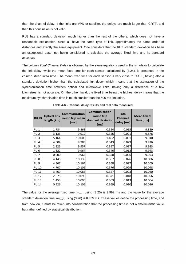
63
than the channel delay. If the links are VPN or satellite, the delays are much larger than CRTT, and
then this conclusion is not valid.
RU3 has a standard deviation much higher than the rest of the others, which does not have a
reasonable explanation, since all have the same type of link, approximately the same order of
distances and exactly the same equipment. One considers that the RU3 standard deviation has been
an exceptional case, not being considered to calculate the average fixed time and its standard
deviation.
The column Total Channel Delay is obtained by the same equations used in the simulator to calculate
the link delay, while the mean fixed time for each sensor, calculated by (3.24), is presented in the
column Mean fixed time. The mean fixed time for each sensor is very close to CRTT, having also a
standard deviation higher than the calculated link delay, which means that the estimation of the
synchronisation time between optical and microwave links, having only a difference of a few
kilometres, is not accurate. On the other hand, the fixed time being the highest delay means that the
maximum synchronisation time is much smaller than the 500 ms limitation.
Table 4-6 - Channel delay results and real data measured.
RU IDOptical link
length [km]
Communication
round trip mean
[ms]
Communication
round trip
standard deviation
[ms]
Total
Channel
delay [ms]
Mean fixed
time[ms]
RU 1 1.784 9.868 0.354 0.015 9.839
RU 2 3.135 9.919 0.326 0.021 9.876
RU 3 5.164 10.003 1.402 0.031 9.940
RU 4 4.604 9.983 0.343 0.029 9.926
RU 5 2.325 9.957 0.357 0.017 9.923
RU 6 1.322 9.967 0.346 0.012 9.943
RU 7 0.000 9.964 0.350 0.006 9.953
RU 8 4.145 10.139 0.367 0.026 10.086
RU 9 4.367 10.164 0.358 0.027 10.109
RU 10 4.707 10.106 0.376 0.029 10.048
RU 11 3.469 10.086 0.327 0.023 10.040
RU 12 2.575 10.093 0.371 0.018 10.056
RU 13 1.453 10.090 0.363 0.013 10.064
RU 14 0.926 10.106 0.369 0.010 10.086
The value for the average fixed time, , using (3.25) is 9.992 ms and the value for the average
standard deviation time, , using (3.26) is 0.355 ms. These values define the processing time, and
from now on, it must be taken into consideration that the processing time is not a deterministic value
but rather defined by statistical distribution.
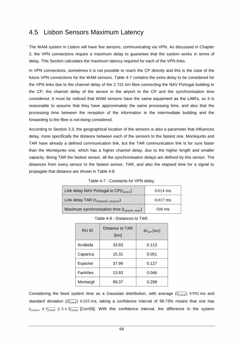
64
4.5 Lisbon Sensors Maximum Latency
The WAM system in Lisbon will have five sensors, communicating via VPN. As discussed in Chapter
2, the VPN connections require a maximum delay to guarantee that the system works in terms of
delay. This Section calculates the maximum latency required for each of the VPN links.
In VPN connections, sometimes it is not possible to reach the CP directly and this is the case of the
future VPN connections for the WAM sensors. Table 4-7 contains the extra delay to be considered for
the VPN links due to the channel delay of the 2.721 km fibre connecting the NAV Portugal building to
the CP, the channel delay of the sensor in the airport to the CP and the synchronisation time
considered. It must be noticed that WAM sensors have the same equipment as the LAM‟s, so it is
reasonable to assume that they have approximately the same processing time, and also that the
processing time between the reception of the information in the intermediate building and the
forwarding to the fibre is not being considered.
According to Section 3.3, the geographical location of the sensors is also a parameter that influences
delay, more specifically the distance between each of the sensors to the fastest one. Montejunto and
TAR have already a defined communication link, but the TAR communication link is for sure faster
than the Montejunto one, which has a higher channel delay, due to the higher length and smaller
capacity. Being TAR the fastest sensor, all the synchronisation delays are defined by this sensor. The
distances from every sensor to the fastest sensor, TAR, and also the elapsed time for a signal to
propagate that distance are shown in Table 4-8.
Table 4-7 - Constants for VPN delay.
Link delay NAV Portugal to CP( ) ms
Link delay TAR ( ) ms
Maximum synchronisation time ( ) ms
Table 4-8 - Distances to TAR.
RU ID Distance to TAR
[km]
Arrábida 33.83 0.113
Caparica 15.31 0.051
Espichel 37.99 0.127
Fanhões 13.93 0.046
Montargil 89.37 0.298
Considering the fixed system time as a Gaussian distribution, with average ( ) ms and
standard deviation ( ) ms, taking a confidence interval of 99.73% means that one has
[Corr09]. With this confidence interval, the difference in the system
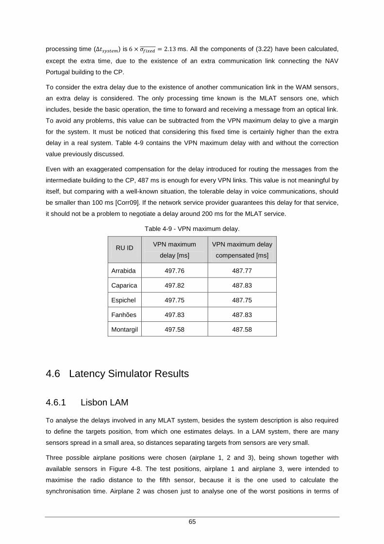
65
processing time ( ) is ms. All the components of (3.22) have been calculated,
except the extra time, due to the existence of an extra communication link connecting the NAV
Portugal building to the CP.
To consider the extra delay due to the existence of another communication link in the WAM sensors,
an extra delay is considered. The only processing time known is the MLAT sensors one, which
includes, beside the basic operation, the time to forward and receiving a message from an optical link.
To avoid any problems, this value can be subtracted from the VPN maximum delay to give a margin
for the system. It must be noticed that considering this fixed time is certainly higher than the extra
delay in a real system. Table 4-9 contains the VPN maximum delay with and without the correction
value previously discussed.
Even with an exaggerated compensation for the delay introduced for routing the messages from the
intermediate building to the CP, 487 ms is enough for every VPN links. This value is not meaningful by
itself, but comparing with a well-known situation, the tolerable delay in voice communications, should
be smaller than 100 ms [Corr09]. If the network service provider guarantees this delay for that service,
it should not be a problem to negotiate a delay around 200 ms for the MLAT service.
Table 4-9 - VPN maximum delay.
RU ID VPN maximum
delay [ms]
VPN maximum delay
compensated [ms]
Arrabida 497.76 487.77
Caparica 497.82 487.83
Espichel 497.75 487.75
Fanhões 497.83 487.83
Montargil 497.58 487.58
4.6 Latency Simulator Results
4.6.1 Lisbon LAM
To analyse the delays involved in any MLAT system, besides the system description is also required
to define the targets position, from which one estimates delays. In a LAM system, there are many
sensors spread in a small area, so distances separating targets from sensors are very small.
Three possible airplane positions were chosen (airplane 1, 2 and 3), being shown together with
available sensors in Figure 4-8. The test positions, airplane 1 and airplane 3, were intended to
maximise the radio distance to the fifth sensor, because it is the one used to calculate the
synchronisation time. Airplane 2 was chosen just to analyse one of the worst positions in terms of

66
coverage, which is only covered by 5 sensors, according to the coverage analysis in Figure D.1.
As explained in the Section 3.2, the individual coverage must be included to define the test file,
besides the choice of the locations. The global input file for these test positions is shown in Table
4-10, and the coverage for each point was accomplished by comparing the test positions with the
coverage maps from Figure D.2 to Figure D.4. For each sensor, if the column contains “1” it means
that this position is covered, and “0” otherwise.
Adding the test file with the Lisbon LAM system description in Table 4-1, the simulator generates the
output file, the most important information being summarised in Table 4-11. As expected with small
radio distances and small link lengths, delays are very small compared to the maximum
synchronisation time, which is 500 ms in this case. In practice, for a LAM, there is no influence from
the communication link length and the distance from the airplane to the sensors.
Figure 4-8 - Test positions for Lisbon LAM
Table 4-10 - Lisbon LAM tests input file.
Test PositionLatitude
[DD° MM'SS"]
Longitude
[DD° MM'SS"]01 02 03 04 05 06 07 08 09 10 11 12 13 14
airplane 1 38°46'36.40"N 9° 8'18.06"W 1 1 1 1 0 1 1 1 1 1 1 1 1 1
airplane 2 38°46'47.00"N 9° 7'47.02"W 1 0 0 0 1 0 0 0 0 0 1 1 0 1
airplane 3 38°47'8.95"N 9° 8'0.86"W 1 1 1 1 0 0 1 1 0 1 1 1 1 1
Table 4-11 - LAM results
Test Position Fastest sensor
[ID]
Slowest sensor
[ID]
Synchronization
time[ms]
airplane 1 7 1 0.016
airplane 2 14 11 0.016
airplane 3 7 2 0.020
This system has the specificity of having all communication links with the same capacity, 100 Mbps,
so the link transmission delay is very small. For the delays calculated from this test positions, it may
be assumed that even testing for every possible position in the airport, the maximum synchronisation
time based on the propagation time in the air and optical fibre is irrelevant. The sensor‟s processing
time was not considered, because it is assumed that they all are approximately the same.

67
4.6.2 Lisbon WAM
As discussed in Chapter 3, there are differences between the LAM and WAM analysis. One of the
differences is in the test positions, and another in the system‟s description. In this Section the delays
expected in the Lisbon WAM system are calculated and discussed. To define the test positions of the
airplanes in a WAM system, the flight routes must be defined. Figure 4-9 contains the representation
of the positions to test, which are better described in Annex A. In Figure 4-9 and every airspace maps
used in this thesis, the coordinates displayed start by the direction, meaning N/S or E/W and then
degrees, minutes and seconds separate by a space.
Considering that a given test route, the declination angle must be estimated. For this, a random
section was chosen in the map, between DEKUS and MAGUM, with coordinates 38°00‟55” N,
10°00‟00” W and 39°10‟03” N, 8°23‟33” W respectively, which has a magnetic angle of 51°. Using
(3.27) the real angle is 47.5°, and from (3.26) the magnetic declination is approximately 3.5°W.
Figure 4-9- Tests for Lisbon WAM [NAV10].
Another test, not included in Figure 4-9, is the approach to the runway, in the most used one in the
Lisbon airport, which is described not on the flight routes map but in Figure 3-8. With all the variables
to describe the test positions, the file to include in the simulator is shown in Table 4-12. The
description of this system is partially given in Table 4-2, and missing column from the description
being the maximum latency of the VPN links.
Two results for the VPN maximum delay could be considered; the maximum latency calculated in
Section 4.4, 487 ms, or a reasonable value that a service provider offers. The value of 487 ms is
exaggerated, and this type of delay is only expected in satellite links. A reference value obtained from
[NAV11] for a VPN link is a round trip delay of 50 ms with an average jitter of 25 ms. The total delay of
the link is 50 ms taking into account the jitter deviation, because the delay is only one way and not a
round trip time.

68
For the approach, two extra sensors are used, RU04 and RU13 from Lisbon LAM, and their coverage
is set to approach, meaning that they only cover the approach test position. The output gives two
results: the total link delay for each sensor without taking the overall MLAT processing time into
consideration; the equivalent to the LAM analysis, giving for each position the covering sensors and
the synchronisation time.
Table 4-12- Tests input file for Lisbon WAM.
ID TypeInitial
Latitude
Initial
Longitude Route
Final
Latitude
Final
Longitude Altitude
Final
Altitude
Descent
angle
Test
points
UN745 Route 38°00'55"N 10°0'0"W 51 195 20
Ateca Single Point 38°39'30"N 8°37'21"W 195 1
Espichel Single Point 38°25'27"N 9°11'9"W 195 1
UN975 Section 38°39'30"N 8°37'21"W 38°25'27"N 9°11'9"W 195 20
RWY03 Approach 38°38'24"N 9°12'41"W 27 30 3.31 5.2 20
UN870a Section 38°32'42"N 10°0'0"W 38°53'16"N 9°9'46"W 195 20
UN870b Route 38°53'16"N 9°9'46"W 69 195 20
The channel delay for each sensor, given as an output of the simulator, is shown in Table 4-13. The
link delays in WAM sensors are much larger than the delays for the LAM‟s. Comparing WAM sensors
link delay with the ones used for the LAM, there is a noticeable increase in delay. If the sensor‟s
processing time would be included with the correspondent standard deviation, only the difference
between the VPN links to the proprietary links would be noticed.
Table 4-13 - Lisbon WAM sensors channel delay
Sensor ID Link Delay
[ms]
Arrabida 50.02
Caparica 50.02
Espichel 50.02
Fanhões 50.02
Montargil 50.02
Montejunto 00.36
TAR (RU 11) 00.02
RU 04 00.03
RU 13 00.01
The results of the synchronisation time are shown in Figure 4-10. Synchronisation times are very close
to the delay defined for the VPN, as expected. It is also noticed that usually as closer the airplane is
from the faster‟s links, the synchronisation time increases. For instance, in the approach case, when
decreasing the distance to the fastest airport links increases the synchronisation time.
The main result is that even in a WAM with distances around 30 NM there is still no impact of the
propagation delays in the system. Also, this system does not have proprietary links with high delays,
and the synchronisation time is defined by the VPN delays, which are more resilient to errors and are
still very far from the maximum latency allowed.
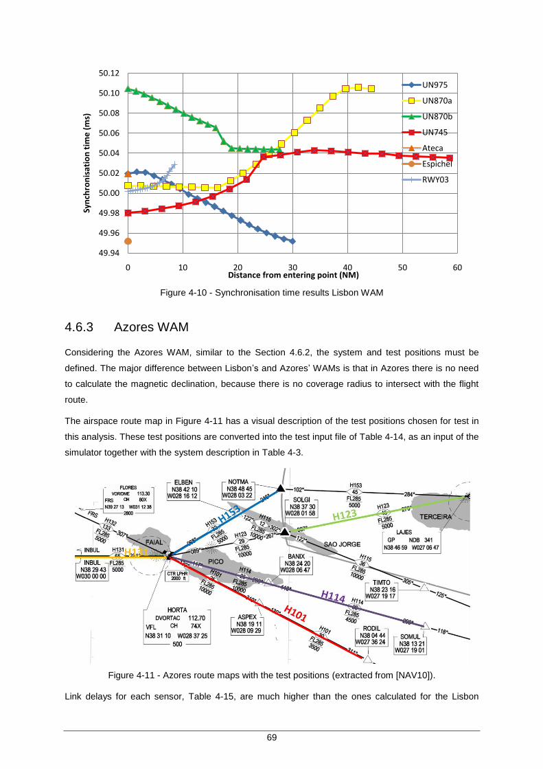
69
Figure 4-10 - Synchronisation time results Lisbon WAM
4.6.3 Azores WAM
Considering the Azores WAM, similar to the Section 4.6.2, the system and test positions must be
defined. The major difference between Lisbon‟s and Azores‟ WAMs is that in Azores there is no need
to calculate the magnetic declination, because there is no coverage radius to intersect with the flight
route.
The airspace route map in Figure 4-11 has a visual description of the test positions chosen for test in
this analysis. These test positions are converted into the test input file of Table 4-14, as an input of the
simulator together with the system description in Table 4-3.
Figure 4-11 - Azores route maps with the test positions (extracted from [NAV10]).
Link delays for each sensor, Table 4-15, are much higher than the ones calculated for the Lisbon
49.94
49.96
49.98
50.00
50.02
50.04
50.06
50.08
50.10
50.12
0 10 20 30 40 50 60
Syn
chro
nis
atio
n t
ime
(m
s)
Distance from entering point (NM)
UN975
UN870a
UN870b
UN745
Ateca
Espichel
RWY03

70
airport, due to the larger distances and smaller capacity of the links. These calculations do not
consider the multi-hop effect, and for instance GS_06 and GS_07 have five hops until reaching the
CP. The extra delay in each hop is not be very large, but considering the small delays calculated in
these analyses, it may have a large influence.
Table 4-14 - Simulator input tests for WAM Azores
ID TypeInitial Latitude
[DD/MM.MMM]
Initial
Longitude
[DD/MM.MMM]
Final Latitude
[DD/MM.MMM]
Final
Longitude
[DD/MM.MMM]
Test
points
Horta Single Point 38°31'10"N 28°37'25"W 1
H153 (HRT-NMA) Section 38°31'10"N 28°37'25"W 38°48'45"N 28°3'22"W 20
H101 (HRT-RDL) Section 38°31'10"N 28°37'25"W 38°4'44"N 27°36'24"W 20
H123 (SLG-LJS) Section 38°37'30"N 28°1'58"W 38°46'59"N 27°06'47"W 20
H114(HRT-SML) Section 38°31'10"N 28°37'25"W 38°13'21"N 27°19'1"W 20
H131(HRT-IBL) Section 38°31'10"N 28°37'25"W 38°29'43"N 30°0'0"W 20
Table 4-15 - Azores sensors channel delay.
Sensor ID link delay [ms]
GS_00 4.43
GS_01 2.21
GS_02 2.25
GS_03 6.70
GS_04 11.30
GS_05 6.78
GS_06 11.23
GS_07 11.55
GS_08 9.09
GS_09 9.22
GS_10 9.02
In this system, no coverage analysis has been performed, so the synchronisation time only takes into
consideration the fastest sensors.
Figure 4-12 contains the test analysis performed with the corresponding synchronisation times. In this
analysis, there is also no concern about the synchronisation delay, because it is much smaller than
the maximum one allowed by the system. This system has a much higher link delay compared to
Lisbon‟s LAM, because links capacities are much smaller, there is a higher number of hops in most of
the links, and links capacity is much lower than optical fibres‟ 100Mbps. Furthermore, it must also be
noticed that in this simulation all sensors in the network are able to forward the message within time to
the CP.
This summarises the analysis of the different networks. To finalise the study of the delay influence in
the system, Section 4.6.4 contains a global view of the different parameters that influence it.

71
4.40
4.45
4.50
4.55
4.60
4.65
4.70
4.75
0 10 20 30 40 50 60 70
Syn
chro
niz
atio
n t
ime
(ms)
Distance from entering point (NM)
H101 (HRT-RDL)
H123 (SLG-LJS)
H114(HRT-SML)
H131(HRT-IBL)
H153 (HRT-NMA)
Figure 4-12- Azores Synchronisation time results.
4.6.4 Overall Multilateration Systems Analysis
After showing the results for the three systems considered, Lisbon‟s LAM and WAM, and Azores‟
WAM, an assessment of the overall MLAT concerning the delay analysis is in order.
The Latency requirements are easily accomplished with any system, but there are some parameters
that also influence the synchronisation time and have not been considered, i.e., standard deviation of
the MLAT system processing time, analysed in Section 4.2, and the extra delay when there are hops
in the communication link. There are five different delay components, air and link propagation time,
transmission time, standard deviation of the system processing time, and the influence of the number
of hops.
The air propagation delay has a speed approximated by the speed of light, Figure 4-13 showing this
delay as a function of distance. For Lisbon‟s LAM, air distances are very small, at most around 4.5 km,
which is approximately the largest dimension in the airport; for this specific case, the propagation time
is much less than 0.1 ms. In the WAM scenario, even having distances that can go above 200 km, the
influence of the synchronisation time is limited by the distance between the sensors as shown in
Section 3.3. For Lisbon‟s WAM, this limitation is worse between Montargil and Espichel, 112 km, and
in Azores‟ WAM is approximately 120 km between GS_00 and GS_09. With these distances, the
maximum air propagation delay difference is not higher than 0.5 .
The link propagation speed depends on the type of link, and can be approximately for an
optical fibre or the speed of light for a microwave link, but the situation is similar to the air propagation
delay, considering that the links distances are also at most a few hundreds of kilometres. In the
analysed scenarios, the highest link length is in Azores with 184.66 km, and the difference between
the shortest and longest is less than 180 km. From Figure 4-13, in this last case, the maximum delay
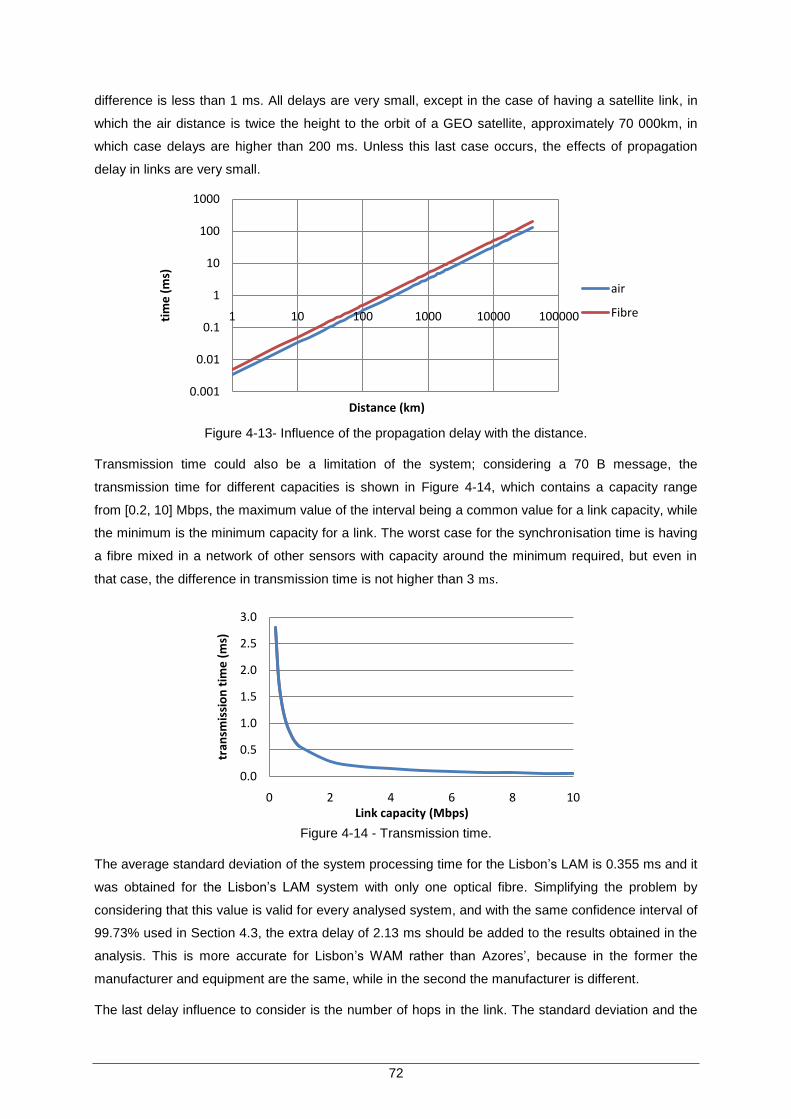
72
difference is less than 1 ms. All delays are very small, except in the case of having a satellite link, in
which the air distance is twice the height to the orbit of a GEO satellite, approximately 70 000km, in
which case delays are higher than 200 ms. Unless this last case occurs, the effects of propagation
delay in links are very small.
Figure 4-13- Influence of the propagation delay with the distance.
Transmission time could also be a limitation of the system; considering a 70 B message, the
transmission time for different capacities is shown in Figure 4-14, which contains a capacity range
from [0.2, 10] Mbps, the maximum value of the interval being a common value for a link capacity, while
the minimum is the minimum capacity for a link. The worst case for the synchronisation time is having
a fibre mixed in a network of other sensors with capacity around the minimum required, but even in
that case, the difference in transmission time is not higher than 3 .
Figure 4-14 - Transmission time.
The average standard deviation of the system processing time for the Lisbon‟s LAM is 0.355 ms and it
was obtained for the Lisbon‟s LAM system with only one optical fibre. Simplifying the problem by
considering that this value is valid for every analysed system, and with the same confidence interval of
99.73% used in Section 4.3, the extra delay of 2.13 ms should be added to the results obtained in the
analysis. This is more accurate for Lisbon‟s WAM rather than Azores‟, because in the former the
manufacturer and equipment are the same, while in the second the manufacturer is different.
The last delay influence to consider is the number of hops in the link. The standard deviation and the
0.001
0.01
0.1
1
10
100
1000
1 10 100 1000 10000 100000tim
e (
ms)
Distance (km)
air
Fibre
0.0
0.5
1.0
1.5
2.0
2.5
3.0
0 2 4 6 8 10
tran
smis
sio
n t
ime
(m
s)
Link capacity (Mbps)

73
average processing time, besides the MLAT system processing time, also includes the delays of
forwarding the information to the link and receiving it, in an optical link. It is not possible to separate
these two parts of the delay, so they must be considered together, and there are three cases in which
an error is made:
only one hop is used, not being an optical fibre;
more than one hop is used, but one of them is an optical fibre;
more than one hop is used, and none of them is an optical fibre.
In the first case, the time difference should be very small, because the optical or microwave links
transmitter/receivers do not differ a lot in terms of delay.
In the second case, it may be considered that the standard deviation and the average of the MLAT
processing time considers the extra delays of one optical link and the system itself, but does not
consider any other delay of the remaining links. For each hop, the time delay considered was
calculated by the propagation delay and the transmission time in (2.6), but there is the extra delay of
receiving the message in an intermediary point, and reading at least the headers to forward the
message correctly.
Finally, the third case is approximately the sum of the last two, and even if no optical links are used, it
may be considered that the delay in one of them is included in the average and standard deviation of
the system processing time. Concerning the rest of the hops, an assessment of the delay not
considered for each extra hop should be done.
For now, it is not possible to get delay results from MLAT systems implemented with more than one
hop, so this value is not possible to estimate. If there were data available, it would be possible to
compare two different links with a different number of hops, and from that to retrieve an estimation of
the extra delay per hop. This extra delay would only be considered for the total number of hops minus
one, because the delay of only one hop has already been considered.
It is arguable that the extra delay by considering the processing time on each hop is quite small, but so
are the other delays involved in the system. Table 4-16 contains the summary of each of the
components and its possible influence of the synchronisation time. The maximum delay is calculated
as the difference between the minimum and maximum value of the considered values. All parameters
that influence the delay are quite small compared to the synchronisation delay, except the satellite and
only in this situation it is possible not to consider the hop effect.
On the one hand, every small delays need to be considered in order to have an accurate simulator but
on the other, all of these values are extremely small, as expected, and will not have any influence in
the MLAT system.
This Section summarised the complete assessment of the possible telecommunication links and their
effect in the MLAT systems already installed or any other to be developed.

74
Table 4-16 - Summary of the delays involved.
Delay component Considered limit Maximum delay
Air [0, 150] km
Fibre/Microwave link propagation [0, 200] km
Satellite propagation [0, 70 000] km
Transmission [0.2, 10] Mbps
Standard deviation MLAT 99.73% ( )
Hops unknown unknown
4.7 North of Portugal Multilateration study
4.7.1 Study Data
A preliminary study for a MLAT WAM system is presented, for the North of Portugal, the area
delimited by the red line in Figure 4-15, where Porto‟s airport TMA is also included the. The TMA is a
very important area, because the surveillance has more restrictive requirements, including the
requirements studied in Section 4.3 for the tracking probabilities. The defined area for the TMA can be
retrieved from [NAV10].
Figure 4-15 - North region to cover.
The study considers some sensors location proposals with different coverage goals, and analyses the
tolerable delay and the required capacity for the links. Altitude coverage requirements are different
within the entire region, but this study, being preliminary, considers FL100.
The first step in the study was to collect information for possible sensors location, and complete an
individual coverage analysis for each one of them. Twenty sensors obtained from [NAV11] were

75
tested, and the individual coverage maps, obtained from the coverage simulator, are shown in
Annex E.
As explained in Section 3.5, two different methods to address sensors importance were proposed:
qualitative and quantitative evaluations. Table 4-17 contains the qualitative evaluation for the tested
sensors, while Table 4-19 contains the quantitative one.
Table 4-17 - Qualitative evaluation of the sensors.
RU IDViana do
CasteloBraga Porto Aveiro Viseu Vila Real Guarda Bragança Porto TMA
Porto Locator Total Total Total Total HalfSW 0 0 0 Total-NE
Porto NDB Total Total Total Total Total-E Total 0 HalfW Total
Viseu VOR-DME 0 0 Total Total Total 0 Total Half S HalfSE
Braganca 0 0 0 0 0 0 0 Total-SW 0
Ovar Tacan Total Total Total Total HalfW HalfW 0 0 Total-NE
Sensor 1 Total Total Total Total Total Total Total-SE HalfSW Total
Sensor 2 Total Total Total Total Total-NE HalfW 0 0 Total-NE
Sensor 3 Total Total Total Total-W Total-W Total 0 Half NW Total-SW
Sensor 4 Total Total Total Total Total Total Total Total-NE Total
Sensor 5 Total Total Total Total Total Total-NE Total HalfSW Total
Sensor 6 Total-NW Total Total Total-S Total Total Total Total Total-NW
Sensor 7 Total Total Total Total Total Total Total Total Total
Sensor 8 HalfE 0 0 0 HalfE HalfNW HalfNW Total 0
Sensor 9 Total Total Total Total Total Total Total Total Total
Sensor 10 Total Total Total Total Total Total 0 HalfW Total
Sensor 11 Total Total Total Total Total Total Total Total Total
Sensor 12 0 Total Total HalfN Total-SW Total Total Total-N HalfE
Sensor 13 Total-NW Total Total Total Total Total Total Total Total-NW
Sensor 14 Total-NE Total Total Total Total HalfS Total Total-NW Total-SW/N
Braganca VOR 0 0 0 0 0 0 Total-SW Total 0
To define the quantitative evaluation, districts areas were taken from [IGP10], but for the districts of
Aveiro, Viseu and Guarda, the considered area is the intersection between the desired coverage,
Figure 4-15, and the district itself; the considered percentage of area covered in each of the districts
was 75%, 85% and 40% for Aveiro, Viseu and Guarda, respectively. The considered areas for each
district are shown in Table 4-18, which were the values used to calculate the percentage of coverage
area, using (3.42). The parameter that gives the percentage of the total coverage area is in the last
column of Table 4-18, under utility. The percentage of coverage in each district is also shown.
For both analyses, the evaluation was done by observation, being used to support the choice of
locations. In order to have more accurate values for the covered area with a certain set of sensors, the
coverage maps in Google Earth must be used. With this information concerning the coverage for
some possible sites, four analyses with different goals are developed in the rest of Section 4.7.

76
Table 4-18 - Districts areas.
District Total area Considered area
Aveiro 2801 2101
Braga 2706 2706
Bragança 6599 6599
Guarda 5535 2214
Porto 2332 2332
Viana do Castelo 2219 2219
Vila Real 4308 4308
Viseu 5010 4258
Table 4-19 - Quantitative evaluation of the sensors.
4.7.2 First Proposal
It is a fact that the minimum number of sensors to execute the TDOA algorithm is at least 4 for a 3D
localisation, as explained in Section 2.2. This minimum number of sensors is increased to 5, in order
to have redundancy in this critical system. Considering these facts, an initial study is to know how
many sensors are required to provide at least 5 sensors covering every location. The first coverage
RU IDViana do
CasteloBraga Porto Aveiro Viseu Vila Real Guarda Bragança Utility
Porto Locator 100% 95% 100% 100% 70% 10% 0% 0% 47.25%
Porto NDB 100% 100% 100% 100% 95% 100% 5% 30% 74.06%
Viseu VOR-DME 0% 0% 100% 100% 100% 0% 100% 40% 50.66%
Braganca 0% 0% 0% 0% 0% 0% 0% 80% 19.74%
Ovar Tacan 100% 100% 100% 100% 70% 30% 0% 0% 50.98%
RU 1 100% 100% 100% 100% 100% 100% 95% 50% 87.25%
RU 2 100% 100% 100% 100% 90% 40% 10% 0% 56.61%
RU 3 100% 100% 95% 95% 70% 100% 0% 60% 76.24%
RU 4 100% 100% 100% 100% 100% 100% 100% 80% 95.06%
RU 5 100% 100% 100% 100% 100% 95% 100% 50% 86.85%
RU 6 95% 100% 100% 75% 98% 100% 100% 100% 97.30%
RU 7 100% 100% 100% 100% 100% 100% 100% 100% 100.00%
RU 8 30% 0% 0% 0% 20% 70% 50% 100% 45.77%
RU 9 100% 100% 100% 98% 100% 100% 100% 100% 99.84%
RU 10 100% 100% 100% 100% 100% 100% 20% 40% 78.57%
RU 11 100% 100% 100% 100% 100% 100% 100% 100% 100.00%
RU 12 0% 95% 100% 40% 90% 95% 100% 80% 79.15%
RU 13 90% 100% 100% 100% 100% 100% 100% 100% 99.17%
RU 14 80% 100% 100% 100% 100% 55% 100% 80% 86.15%
Braganca VOR 0% 0% 0% 0% 10% 15% 80% 100% 35.32%
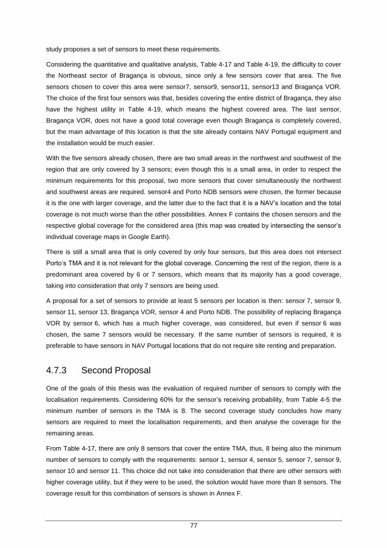
77
study proposes a set of sensors to meet these requirements.
Considering the quantitative and qualitative analysis, Table 4-17 and Table 4-19, the difficulty to cover
the Northeast sector of Bragança is obvious, since only a few sensors cover that area. The five
sensors chosen to cover this area were sensor7, sensor9, sensor11, sensor13 and Bragança VOR.
The choice of the first four sensors was that, besides covering the entire district of Bragança, they also
have the highest utility in Table 4-19, which means the highest covered area. The last sensor,
Bragança VOR, does not have a good total coverage even though Bragança is completely covered,
but the main advantage of this location is that the site already contains NAV Portugal equipment and
the installation would be much easier.
With the five sensors already chosen, there are two small areas in the northwest and southwest of the
region that are only covered by 3 sensors; even though this is a small area, in order to respect the
minimum requirements for this proposal, two more sensors that cover simultaneously the northwest
and southwest areas are required. sensor4 and Porto NDB sensors were chosen, the former because
it is the one with larger coverage, and the latter due to the fact that it is a NAV‟s location and the total
coverage is not much worse than the other possibilities. Annex F contains the chosen sensors and the
respective global coverage for the considered area (this map was created by intersecting the sensor‟s
individual coverage maps in Google Earth).
There is still a small area that is only covered by only four sensors, but this area does not intersect
Porto‟s TMA and it is not relevant for the global coverage. Concerning the rest of the region, there is a
predominant area covered by 6 or 7 sensors, which means that its majority has a good coverage,
taking into consideration that only 7 sensors are being used.
A proposal for a set of sensors to provide at least 5 sensors per location is then: sensor 7, sensor 9,
sensor 11, sensor 13, Bragança VOR, sensor 4 and Porto NDB. The possibility of replacing Bragança
VOR by sensor 6, which has a much higher coverage, was considered, but even if sensor 6 was
chosen, the same 7 sensors would be necessary. If the same number of sensors is required, it is
preferable to have sensors in NAV Portugal locations that do not require site renting and preparation.
4.7.3 Second Proposal
One of the goals of this thesis was the evaluation of required number of sensors to comply with the
localisation requirements. Considering 60% for the sensor‟s receiving probability, from Table 4-5 the
minimum number of sensors in the TMA is 8. The second coverage study concludes how many
sensors are required to meet the localisation requirements, and then analyse the coverage for the
remaining areas.
From Table 4-17, there are only 8 sensors that cover the entire TMA, thus, 8 being also the minimum
number of sensors to comply with the requirements: sensor 1, sensor 4, sensor 5, sensor 7, sensor 9,
sensor 10 and sensor 11. This choice did not take into consideration that there are other sensors with
higher coverage utility, but if they were to be used, the solution would have more than 8 sensors. The
coverage result for this combination of sensors is shown in Annex F.

78
In this proposal, the intersection of Porto‟s TMA with the coverage is the most important result, which
is why the TMA is overlapped with the global coverage. There is a small TMA area that is only covered
by seven sensors, but it is negligible, so no more sensors were added to this proposal. Considering
that this study only considers eight sensors, the area covered by eight or seven is very large, and the
only area that does not meet the first proposal requirements is the Bragança Northeast.
The study to guarantee eight sensors covering the TMA cannot be final because not all requirements
of a MLAT system are met, but it is helpful to complete the last study, which improves this second
proposal.
4.7.4 Third Proposal
After presenting the first two proposals, it was defined that a useful study would be to add three
sensors to the second proposal, increasing the total number of sensors to eleven. The sensors to add
are the ones with more coverage utility from the remaining set.
The third proposal considers the sensors from the second and in addition will add sensors sensor 6,
sensor 13 and sensor 14, which are the sensors with higher coverage area. Sensor 6 and sensor 13
cover the entire district of Bragança, and sensor 14 is the remaining sensor with the largest total
coverage. Annex F contains the global coverage of this proposal.
Including two sensors that cover Bragança entirely, and another that gives a partial coverage,
improves a lot the global coverage of the North region. The TMA is also better covered with 11 or 10
sensors, except in a few small areas in the North border that are only covered by 9.
This proposal could be improved if the Porto NDB sensor was replaced by sensor 12, this way the
system would have the eleventh best sensors in terms of total coverage. However, this replacement
was not considered, because the difference in approximate coverage is around 5%. Another reason is
that Porto NDB, besides being a NAV Portugal site, is also in a very strategic place to cover the area
near the airport.
All requirements are met with this choice of sensors, every region has at least 5 sensors and the TMA
is covered by more than 8 sensors. Except for small areas in the TMA and Bragança, the redundancy
of this system is 2. This means that even if sensor sensor 7 and sensor 9 fail, whose coverage utility is
100%, the requirements are still fulfilled in the majority of the area to cover.
4.7.5 Fourth Proposal
In terms of global coverage the last proposal is better than any other arranged combination, but the
fact is that Bragança is not a district with a high frequency of airplanes, on the contrary, the traffic in
this region is very small and it is preferable to cover the coast and the TMA better rather than that
region. Due to this fact, one analysed the possibility to place two sensors that provide the minimum
coverage to Bragança, and another near the coast, even if it is not the one with the largest coverage.
Another motivation to replace one sensor from the last proposal by another in the coast is to have

79
more spatial diversity. This matter has not been discussed in this thesis, but the accuracy of the MLAT
system depends on the sensors position in relation to the airplane. If an airplane is covered by 5
sensors but they are all in a straight line, the uncertainty of the calculated position is much higher than
if the airplane is in-between the same number of sensors. Preventing this situation, whose effects
have not been considered, a sensor placed in the coast increases the spatial diversity.
The sensor to replace must be one that does not cover the northeast sector of Bragança, and that
does not have a high global coverage compared to the others, sensor 14 being chosen. The sensor to
add in the southwest region with the largest global coverage is Ovar Tacan, which has two
advantages: it is much separated from Porto NDB, which is also located in the coast, and it is located
in a military site, which is probably better than having to rent the site from a telecommunications
operator or even building a new one. Annex F contains the global coverage for the last proposal.
By comparing the third with the fourth proposal coverage map, it is observable that the third proposal
has a better overall coverage of the region, especially in Bragança. On the other hand, this last
proposal improves the coverage in the cost and the TMA. Taking into consideration that the East area
is not as important as the coast, this last proposal should be given more value.
This proposal finalises the coverage study of the North region of Portugal. Still, some more
considerations in terms of communication links are discussed in the Section 4.7.6.
4.7.6 Global Analysis
Four different sensors combinations with different objectives have been proposed, but the only
complete proposal to consider for the final implementation are the third and fourth. Besides the
coverage analysis, it is also important to assess other requirements considered in this thesis, like the
maximum latency and the required capacity for the communication links.
The required capacity for the links is directly related to the expected traffic in the region. If the
maximum expected traffic in the defined region is 250 airplanes, then, as concluded in Section 4.2,
each link should have at least 275.7 kbps. Even though it is possible to define the maximum capacity
required for 250 airplanes, it mainly depends on each sensor individually. The coverage figures in
Annex E only contain the North area, but their coverage for FL100 is much wider than that, and
considering that most of the airplanes travel in higher routes, then, this coverage will also increase.
The conclusion is that to determine the capacity required for each link, one should take the individual
coverage of the sensor into account. The solution of reducing the sensor‟s range may not be effective,
and may decrease the system‟s efficiency. In case the sensor is placed in the limits of the region to
cover, reducing the range of the sensor the required capacity is also reduced, but at the cost of
reducing their effective covered area. In the third and fourth proposal coverage maps, most of the
sensors are in this situation, because many are located near the border with Spain. A solution not to
limit the effective covered area is to use sector antennas, used often in mobile networks. Using sector
antennas for the sensors places near the border, the sector including the area not to cover can have a
minimum range, while the other sectors have the maximum range allowed. If this is possible to

80
implement, it would solve the link capacity problem, and also be energy efficient, because no energy
would be spent covering a region that is not NAV Portugal‟s responsibility.
Concerning the maximum latency for the communication links, the analysis is the same used to
assess the required latency for the WAM sensors in Lisbon. In this case, there is still no specific
location for the CPS, but probably it will be located near Porto‟s airport. In this situation, the fastest link
would be Porto NDB, because it is a station with surveillance equipment and is certainly connected to
the airport by a fast private communication link. By using (3.22), it is possible to estimate the
maximum delay for every other link compared to the fastest one. The extra delay in the air and the
MLAT processing time are the only parameters that influence the delay, not depending on the
communication link.
By using Google Earth, the maximum distance that separates a pair of sensors in that region is around
250 km, which corresponds to the distance from the Southwest end to the Northeast. According to
Figure 4-13, the extra delay of this component is around 1 ms. The MLAT processing time standard
deviation is the same used in the Lisbon VPN, and for a confidence interval of 99.73 %, the maximum
difference in time is 2.13 ms.
As a final conclusion, there are no problems concerning the delays, and if a VPN connection is used
for all sensors, the tolerable delay can be very close to the maximum allowed. Any service provider
operator will easily supply a maximum delay of 200 ms, which is higher than the current values
tolerable for mobile communications. All private links should be used, but in case none is available,
renting a VPN link is a solution.

81
Chapter 5
Conclusions
5 Conclusions
This chapter finalises this work, summarising conclusions and pointing out aspects to be developed in
future work.

82
This thesis consists of a study of multilateration systems requirements and limitations in Portugal, in
Lisbon and Azores, and the design of a new system for the North of the country.
Chapter 2 focuses in four different subjects: messages used in air surveillance, introduction to
multilateration systems, the state of the art, and the description of possible telecommunications links
to use. Concerning the messages used, the most important information is concerning their size and
sending rate which are used to calculate the capacity of the links. The multilateration system
description is important to provide the basic knowledge of how multilateration works. Finally, the
telecommunication links Section, used to develop the latency model, explaining the delays involved in
each type of link.
In Chapter 3, two models were developed to estimate the delay in a multilateration system and to
analyse the coverage of each sensor. For the latency model, the delays in the links and the possible
distance between the airplane and sensors were implemented in a simulator, which estimates the
delays for a given MLAT system considering the possible routes of the airplanes. The coverage model
is based on the land profile surrounding the sensor and the height of the airplane, which enables the
global coverage calculation. These models were also implemented in a simulator, which is able to
request from the Google servers the information necessary to calculate the global coverage and
represent it in Google Earth.
Beside the discussed models, Chapter 3 also includes some smaller models to estimate the capacity
required in a link, to estimate the maximum allowed delay for a virtual private network link, and finally
to assess the localisation requirements according to the number of sensors. These three models do
not have a simulator, because the calculations are only using one or two equations.
In Chapter 4, by analysing the results in each Section, the overall conclusions from this work can be
divided into two categories, the communication links and the multilateration sensors. The
communication links conclusions are mainly three: the required capacity for the communication links to
support 250 targets is 275.7 kbps, the synchronisation time is not close to the maximum tolerable
delay of 500 ms, and the maximum delay for the VPN links in Lisbon is 487 ms. For a more detailed
analysis of each conclusion:
The average expected traffic is much smaller than the maximum one, but the capacity for it must
at least cope with the traffic generated by the maximum number of targets plus a safety margin
that should also be considered. Concerning the provided headers, for a usage ratio of 90%, a
receiving probability of 40%, and 250 targets, links require 275.7 kbps. The main impact on links
capacity is due to headers.
The delay analysis for each of the implemented systems using the simulator did not presented any
delay problems, as expected. Analysing all the components of delay, and not considering the large
delay of using a satellite link, the largest influence is from the sensors processing time. This delay
has been estimated from the equipment installed in the Lisbon airport, and it has an average fixed
delay and standard deviation smaller than 10 ms and 0.4 ms, respectively.
For the maximum tolerable delay in Lisbon‟s wide area multilateration VPN links, the result is that
487 ms is enough. For normal voice communications the tolerable delay is around 200 ms, which

83
the telecommunications operators have been guaranteeing for a large number of years, hence,
with the technological advances, the maximum delay provided will be much smaller.
The calculated delays are not very accurate, because the standard deviation itself is around the same
order of magnitude as every other component, so even a link that in theory is the fastest, it may be
proven otherwise with real measures. Also, the effect of the processing time in the multi-hop could not
be considered, because measures to conclude about its significance were not available.
Regarding the multilateration sensors, the work is split into two parts: to analyse the localisation
requirements from Eurocontrol, and then to perform a coverage study for the Northern region of
Portugal. Localisation requirements are two, concerning the tracking probability higher than 99 % in
five update intervals, and the continuous tracking probability higher than 97% in one update interval.
The minimum number of sensors required to execute the time difference of arrival algorithm is 3 or 4,
for a 2D or 3D localisation respectively. On the other hand, to comply with the Eurocontrol
requirements and considering that the receiving probability of the sensors is not 100 %, more sensors
are required. To calculate the two localisation requirements, it was considered that the minimum
number of sensors to execute the localisation algorithm is 4 and that the track initiation can be
performed with 2 or 3 consecutive messages. The conclusion is that 4 sensors are never enough to
comply with the requirements in the terminal manoeuvring area and that the requirement more
restrictive is the track initiation. If a 40 % receiving probability is considered, the minimum number of
sensors to cover the terminal manoeuvring area is 8 if three consecutive messages are required to
initiate the track or 7 sensors if only two messages are required.
Four different coverage studies for FL100 have been developed using some sensors locations. From
them it was concluded that:
To provide coverage of 5 sensors per location in the North of Portugal, which is the minimum
requirements for the algorithm plus one extra sensor for redundancy, 7 sensors are required.
To comply with the localisation requirements in the terminal manoeuvring area of Porto, with a
40 % receiving probability and for a track initiation with three messages, 8 sensors are required.
The first two coverage proposals were useful to analyse the impact of the minimum requirements of
the system but a system cannot be implement only respecting the minimum requirements. Following
NAV Portugal indications, two other coverage studies were made to have a more robust system with
the total of 11 sensors. Both analyses guarantee a redundancy of one sensor and to have 8 sensors in
the TMA a redundancy of two sensors.
The effects of the sensor‟s receiving probability affect two critical system requirements, the localisation
probability and the link capacity. For this thesis the main receiving probability considered was around
40 %, but this parameter may change a lot depending on the equipment and conditions. The fact is
that with a small receiving probability the required capacity is smaller, but the number of sensors to
respect the localisation requirements increase. On the other hand, if the receiving probability
increases, the links capacity must increase and the required number of sensors decreases. This
parameter influences a lot the entire system, and it must be carefully analysed.
84
The last note concerns the range of the sensors. All manufacturers have sensors with the capability of
covering 200 NM, meaning that with one sensor there is the possibility of covering almost the entire
country. When an air navigation service provider defines the maximum number of targets, they are
assuming that in the desired area the number of airplanes will not exceed that number. On the other
hand, a sensor may have a large coverage area, and like in Lisbon for the most common flight levels,
above 10 000 feet, the covered area is more than the double of the desired one. In conclusion, if the
range exceeds the desired coverage, the capacity of the link should be increased, or the range can be
limited.
This concludes the analysis performed in the thesis, but still there are future improvements and work
to perform on this subject:
If there are delay measures of a multilateration system, like the one installed in Azores, the effect
of the multi-hop links in the total delay can be better estimated. To have accurate values, it is very
important that this analysis is performed, especially because all delay components involved in this
type of systems have very small values.
Considering the coverage range for flight levels higher than 10 000 feet, it is possible to cover the
entire country with a small set of sensors, instead of having each region independent between
themselves. The multilateration systems analysed consider that the messages can be forward to
different systems, which allows having a common control centre that is able to provide
surveillance to the entire Portuguese airspace, and still have the possibility of forwarding
messages to other control centres. This can become more efficient, because the sensors range
can be maximised and cover a larger area. And it was also shown that the capacity to rent in a
VPN link is small considering the bandwidth that is available nowadays.
The influence of the delay has been discussed, but the accuracy of the system has not. There are
two critical aspects to study the influence in the location accuracy: the sensors geographical
disposition and the number of sensors. It is known that if 5 sensors are all in the same azimuth of
the airplane, the error of the position is much higher than if they have different azimuths. It is
important to quantify this effect, in order to have a better project of the system and reduce the
dependency from the multilateration manufacturers.
If there is the possibility of removing the limitation of the land profile requests used in the
developed simulator, it may be used for lower flight levels and increase its accuracy.
Hopefully the work developed in this thesis is of value to a air navigation service provider. It can give
deeper knowledge to evaluate the manufactures proposals, and compare their proposals with the
expected performance.
All in all, the main goal of this thesis is to be one step forward in recent technologies and to
understand that knowledge is the most powerful weapon that one has.

85
Annex A Latency Simulator Manual
Annex A - Latency Simulator Manual
This Annex presents indications for the use of the simulator with examples of input files and
description of the GUI, two different software were used, Matlab R2007b [MatL11] for the simulator
and Microsoft Office Excel 2007 for the input/output files. The simulator code is only accessible in the
Matlab files.
The application can be started by the executable file or by the Matlab file multilateration.m that
contains the GUI and Figure A.1 is displayed.
Figure A.1 - Simulator GUI.
There are three parameters to define, the cell radius, the declination of the area in question and the
maximum allowed synchronisation time. All of these parameters have default values, mentioned on
the GUI, and to insert a decimal value it must be used the „.‟. The analysis type, WAM or LAM, is
chosen by the option button in the upper left corner.
Pressing the button Select Input File 1 or Select Input File 2, a file select browser like Figure A.2 is
displayed. The first input file must contain the system description and the second the test positions,
some examples are given for both input files bellow.
To run the simulator the Run button must be pressed but it will only run if both input files are selected.
After the second input file is selected it will appear in the GUI a note saying the output name and
another note will appear while the simulator is running, Figure A.3. When the execution ends an
information message is displayed.

86
Figure A.2 - Select file.
Figure A.3 - Output name and simulator status.
The first input file contains the general description of the system, containing all the sensors in the
network, and the complete description of the communication links. The CPS should also be included in
the list of sensors because the cell radius is calculated from its position. The reference transmitters
may be included or not. This description file must be able to fit any possible system if it would be used
only for the Lisbon LAM the input file must contain the information of Table 4-1.
The simulator must considered all communication link types; satellite, optical fibre, microwave link and
VPN. As explained in chapter 2, optical fibres and microwave links are described by its length and
capacity, satellites by their orbit altitude and capacity, and finally VPN by a maximum delay, so the
final input test must include some more categories than Table 4-1. The required headers to include in
the LAM system description file are shown in Table A.1 while the headers for a WAM description file
are shown in Table A.2.
Table A.1 - Headers to include in the LAM system description.
IDEquipment
Type
Latitude
[DD°MM'SS.SS"]
Longitude
[DD°MM'SS.SS"]
Required
Communicati
on Link
Link
Capacity
[Mbps]
Elevation
AGL [m]
Link
length
[km]
Extra
delay
[ms]
The WAM description file has three main differences from the LAM description. First there is the
possibility of using an extra fibre link with a different capacity for any sensor. This difference is
extremely important because the CPS is usually located in the middle of the airport and for WAM
sensors it may be common that the data is received another place before being forward to the CPS.
Second, the hops in a link are considered, and obviously the message must be processed in each
hop. Finally a coverage column will be added for a more specific analysis.
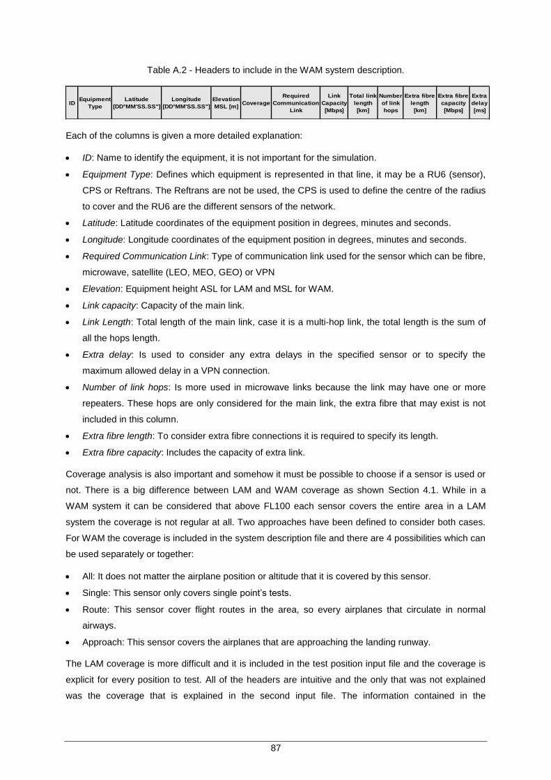
87
Table A.2 - Headers to include in the WAM system description.
IDEquipment
Type
Latitude
[DD°MM'SS.SS"]
Longitude
[DD°MM'SS.SS"]
Elevation
MSL [m]Coverage
Required
Communication
Link
Link
Capacity
[Mbps]
Total link
length
[km]
Number
of link
hops
Extra fibre
length
[km]
Extra fibre
capacity
[Mbps]
Extra
delay
[ms]
Each of the columns is given a more detailed explanation:
ID: Name to identify the equipment, it is not important for the simulation.
Equipment Type: Defines which equipment is represented in that line, it may be a RU6 (sensor),
CPS or Reftrans. The Reftrans are not be used, the CPS is used to define the centre of the radius
to cover and the RU6 are the different sensors of the network.
Latitude: Latitude coordinates of the equipment position in degrees, minutes and seconds.
Longitude: Longitude coordinates of the equipment position in degrees, minutes and seconds.
Required Communication Link: Type of communication link used for the sensor which can be fibre,
microwave, satellite (LEO, MEO, GEO) or VPN
Elevation: Equipment height ASL for LAM and MSL for WAM.
Link capacity: Capacity of the main link.
Link Length: Total length of the main link, case it is a multi-hop link, the total length is the sum of
all the hops length.
Extra delay: Is used to consider any extra delays in the specified sensor or to specify the
maximum allowed delay in a VPN connection.
Number of link hops: Is more used in microwave links because the link may have one or more
repeaters. These hops are only considered for the main link, the extra fibre that may exist is not
included in this column.
Extra fibre length: To consider extra fibre connections it is required to specify its length.
Extra fibre capacity: Includes the capacity of extra link.
Coverage analysis is also important and somehow it must be possible to choose if a sensor is used or
not. There is a big difference between LAM and WAM coverage as shown Section 4.1. While in a
WAM system it can be considered that above FL100 each sensor covers the entire area in a LAM
system the coverage is not regular at all. Two approaches have been defined to consider both cases.
For WAM the coverage is included in the system description file and there are 4 possibilities which can
be used separately or together:
All: It does not matter the airplane position or altitude that it is covered by this sensor.
Single: This sensor only covers single point‟s tests.
Route: This sensor cover flight routes in the area, so every airplanes that circulate in normal
airways.
Approach: This sensor covers the airplanes that are approaching the landing runway.
The LAM coverage is more difficult and it is included in the test position input file and the coverage is
explicit for every position to test. All of the headers are intuitive and the only that was not explained
was the coverage that is explained in the second input file. The information contained in the

88
description file is the same as the tables explaining the multilateration system but the simulator must
work independently of the input and that is the reason of the higher number of columns when
comparing to the system description. One example of each system description, LAM and WAM, are
shown in Table A.3 and Table A.4 respectively. For the WAM system description, the columns
Equipment Type, Latitude and Longitude were hidden but they must appear in the file. Both examples
illustrate most of the possibilities for the different columns and can be used as reference for future
tests to run.
Table A.3 – LAM first input file example.
IDEquipment
Type
Latitude
[DD°MM'SS.SS"]
Longitude
[DD°MM'SS.SS"]
Required
Communicati
on Link
Link
Capacity
[Mbps]
Elevation
AGL [m]
Link
length
[km]
Extra
delay
[ms]
SMR CPS 38° 46'45.66"N 9° 8'22.56"W None Required N/A N/A N/A N/A
X1 RefTran 38° 46'51.3"N 9° 7'55.74"W None Required N/A N/A N/A N/A
RU01 RU6 38°46'51.30"N 9° 7'55.74"W Fibre 100 33 1.784 0
RU02 RU6 38° 47'21.06"N 9° 7'49.26"W Microwave 100 13 3.135 0
RU03 RU6 38°47'51.90"N 9° 7'50.34"W VPN N/A 3 N/A 400
RU04 RU6 38°47'57.18"N 9° 7'35.28"W Satellite 0.2 3 N/A 0
RU05 RU6 38°46'51.78"N 9° 7'45.06"W LEO 0.2 15 N/A 0
RU06 RU6 38°46'41.94"N 9° 7'53.52"W MEO 0.2 20 N/A 0
RU07 RU6 38°46'45.66"N 9° 8'22.56"W GEO 0.2 8 N/A 0
Table A.4 - WAM first input file example.
IDElevation MSL
[m]Coverage
Required
Communic
ation Link
Link
Capacity
[Mbps]
Total link
length
[m]
Number
of link
hops
Extra fibre
length [km]
Extra fibre
capacity
[Mbps]
Extra
delay
[ms]
SMR N/A N/ANone
RequiredN/A N/A N/A N/A N/A N/A
Arrabida 133 all VPN 100 N/A N/A 2.721 100 480
Caparica 105 all VPN 100 N/A N/A 2.721 100 480
Espichel 103 all VPN 100 N/A N/A 2.721 100 480
Fanhões 100 single VPN 100 N/A N/A 2.721 100 480
Montargil 112 route VPN 100 N/A N/A 2.721 100 480
MonteJunto 121approach ; route ;
singlemicrowave 100 47717 2 2.721 100 0
TAR (RU 11)
airport108 approach fibre 100 3469 1 0 0 0
Beside the system description file it is also required to know the airplane test positions because the
total delay of the system also depends on the airplane location. There is also a difference between
LAM and WAM, in the first case airplanes have a very limited set of possible positions and the altitude
is well known while in the WAM they can have flight routes with different altitudes.
The LAM test positions are only be given by a single point, meaning that the airplanes position is a
latitude and longitude without having to add any information concerning the flight altitude. There is a
slight error committed by not considering the transponder AGL height but as there is no fixed

89
transponder height it is not used. In the LAM test file the coverage must be included explicitly,
meaning that for each test position it must include which of the sensors cover that position. An
example of a LAM input test file is shown in Table A. 5. The test file contains three different test
positions each one of them with latitude and longitude coordinates. The columns 01 to 14 represent
each of the sensors ID in the network and the value “1” is used when the sensor covers the test
position and “0” otherwise.
There are four different test positions for a WAM test file:
Single point: It is required to specify the latitude and longitude of the point, the flight level of the
airplane and contain “1” in the column Test Points, otherwise the test are not be performed.
Route: It is required to specify, the coordinates for the initial point, the route angle, the altitude of
the airplane and the number of test points.
Section: It is required to specify, the initial and final point coordinates, the altitude of the airplane
and the number of test points.
Approach: It is required to specify, the coordinated of the beginning of the descent, the route
angle, the initial and final altitude, the descent angle and the number of test points.
Table A.6 contains an example of a WAM test input file with every possible test positions considered.
The coverage of the WAM sensors has been already considered in the system description file.
After running the simulator with both input files, the excel output is created in the same folder as the
test position file under the name “Output_” plus the name of the test position file name. This output file
is also different if the user chose a LAM or WAM analysis. The output for the LAM test file in Table A.
5, is Table A.7. Because the LAM analysis is much smaller and only works with single points, all
delays from the airplane to the CPS, through each of the sensors are presented. Furthermore the
fastest and fifth fastest sensor with the correspondent synchronisation time is shown in the last
columns of the output.
The output for a WAM test file is different from the LAM‟s and depends even though all the results are
presented in the same file, each of the required test positions is presented separately. Table A.8,
Table A.9 and Table A.10 contain the output of a single point, section and approach, respectively. The
route output is not presented because it has the same structure as the section. Starting by the single
point output, the information is equivalent to the LAM‟s but instead of presenting the calculated delay
for each sensor it lists the sensors that arrive within the synchronisation time.
The section and route output are similar to the single point analysis considering each test point
separately. The only difference is that in this output the each analysed point is numbered and its
distance to the initial point is presented. Finally, the approach section differs from the section and
route because it contains a column giving the altitude of the airplane in the correspondent position.
This Annex presented the user manual and the description of the parameters for a future use of the
simulator. It gives a more detailed explanation of the interface but to make changes to it, the section
with the correspondent model and simulator should also be consulted.

90
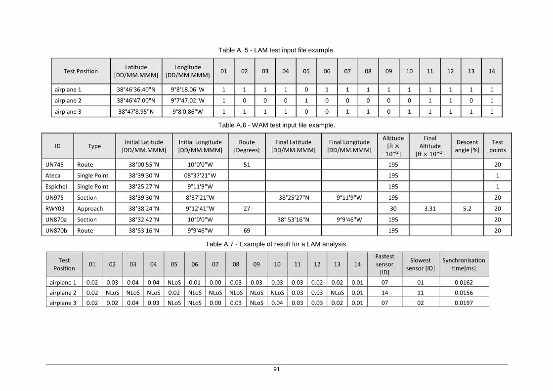
91
Table A. 5 - LAM test input file example.
Test Position Latitude
[DD/MM.MMM] Longitude
[DD/MM.MMM] 01 02 03 04 05 06 07 08 09 10 11 12 13 14
airplane 1 38°46'36.40"N 9°8'18.06"W 1 1 1 1 0 1 1 1 1 1 1 1 1 1
airplane 2 38°46'47.00"N 9°7'47.02"W 1 0 0 0 1 0 0 0 0 0 1 1 0 1
airplane 3 38°47'8.95"N 9°8'0.86"W 1 1 1 1 0 0 1 1 0 1 1 1 1 1
Table A.6 - WAM test input file example.
ID Type Initial Latitude
[DD/MM.MMM] Initial Longitude [DD/MM.MMM]
Route [Degrees]
Final Latitude [DD/MM.MMM]
Final Longitude [DD/MM.MMM]
Altitude [ ]
Final Altitude
[ ]
Descent angle [%]
Test points
UN745 Route 38°00'55"N 10°0'0"W 51
195
20
Ateca Single Point 38°39'30"N 08°37'21"W
195
1
Espichel Single Point 38°25'27"N 9°11'9"W
195
1
UN975 Section 38°39'30"N 8°37'21"W
38°25'27"N 9°11'9"W 195
20
RWY03 Approach 38°38'24"N 9°12'41"W 27
30 3.31 5.2 20
UN870a Section 38°32'42"N 10°0'0"W
38° 53'16"N 9°9'46"W 195
20
UN870b Route 38°53'16"N 9°9'46"W 69
195
20
Table A.7 - Example of result for a LAM analysis.
Test Position
01 02 03 04 05 06 07 08 09 10 11 12 13 14 Fastest sensor
[ID]
Slowest sensor [ID]
Synchronisation time[ms]
airplane 1 0.02 0.03 0.04 0.04 NLoS 0.01 0.00 0.03 0.03 0.03 0.03 0.02 0.02 0.01 07 01 0.0162
airplane 2 0.02 NLoS NLoS NLoS 0.02 NLoS NLoS NLoS NLoS NLoS 0.03 0.03 NLoS 0.01 14 11 0.0156
airplane 3 0.02 0.02 0.04 0.03 NLoS NLoS 0.00 0.03 NLoS 0.04 0.03 0.03 0.02 0.01 07 02 0.0197
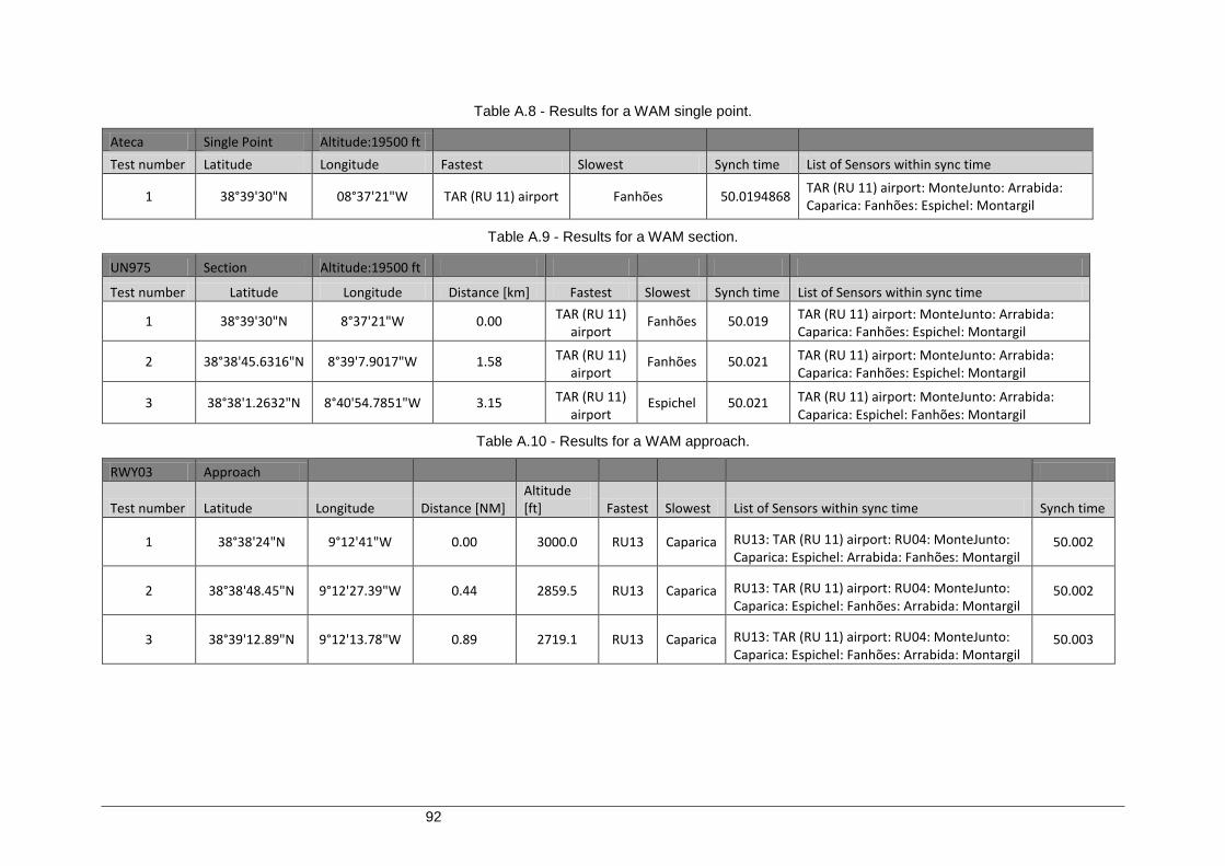
92
Table A.8 - Results for a WAM single point.
Ateca Single Point Altitude:19500 ft Test number Latitude Longitude Fastest Slowest Synch time List of Sensors within sync time
1 38°39'30"N 08°37'21"W TAR (RU 11) airport Fanhões 50.0194868 TAR (RU 11) airport: MonteJunto: Arrabida: Caparica: Fanhões: Espichel: Montargil
Table A.9 - Results for a WAM section.
UN975 Section Altitude:19500 ft
Test number Latitude Longitude Distance [km] Fastest Slowest Synch time List of Sensors within sync time
1 38°39'30"N 8°37'21"W 0.00 TAR (RU 11) airport
Fanhões 50.019 TAR (RU 11) airport: MonteJunto: Arrabida: Caparica: Fanhões: Espichel: Montargil
2 38°38'45.6316"N 8°39'7.9017"W 1.58 TAR (RU 11) airport
Fanhões 50.021 TAR (RU 11) airport: MonteJunto: Arrabida: Caparica: Fanhões: Espichel: Montargil
3 38°38'1.2632"N 8°40'54.7851"W 3.15 TAR (RU 11) airport
Espichel 50.021 TAR (RU 11) airport: MonteJunto: Arrabida: Caparica: Espichel: Fanhões: Montargil
Table A.10 - Results for a WAM approach.
RWY03 Approach
Test number Latitude Longitude Distance [NM] Altitude [ft] Fastest Slowest List of Sensors within sync time Synch time
1 38°38'24"N 9°12'41"W 0.00 3000.0 RU13 Caparica RU13: TAR (RU 11) airport: RU04: MonteJunto: Caparica: Espichel: Arrabida: Fanhões: Montargil
50.002
2 38°38'48.45"N 9°12'27.39"W 0.44 2859.5 RU13 Caparica RU13: TAR (RU 11) airport: RU04: MonteJunto: Caparica: Espichel: Fanhões: Arrabida: Montargil
50.002
3 38°39'12.89"N 9°12'13.78"W 0.89 2719.1 RU13 Caparica RU13: TAR (RU 11) airport: RU04: MonteJunto: Caparica: Espichel: Fanhões: Arrabida: Montargil
50.003

93
Annex B Latency Simulator Flowcharts
Annex B - Latency Simulator Flowcharts
With the latency model developed, to develop the simulator it must also be presented the flowcharts
that created it. They are required to understand the steps of the simulator and its implementation. This
Annex presents the flowcharts for the LAM and WAM simulator, but their description is given in
Section 3.6. The LAM flowchart is presented in Figure B.1 while the WAM‟s is in Figure B.2.
Read System
description
Beginning
Input file with
system description
Read Test
Positions
Input file with test
positions
Calculate link
delay for each
sensor
Number of
positions > 0?
Coverage in the
test pointsYes
Choose 5 fastest
times and
calculate
synchronization
time
Number of
positions -1
Calculate
propagation delay
for each sensor
covered
Finish
Write Output
No
Excel Output
file
List sensors within
maximum
synchronization
time
Figure B.1 – LAM simulator flowchart.

94
Read System
description
Beginning
Input file with
system description
Read Test
Positions
Input file with test
positions
Calculate link
delay for each
sensor
Nº of tests > 0
Calculate the
coordinates of the
landing position
Approach
Calculate the
coordinates of the
points in the
section (number of
test points)
Section
Calculate the
coordinates of the
two Points
intersecting the
coverage raius
Route
Calculate the
propagation delay
for each sensor
Single Point
Finish
Write Output
No
Excel Output
file
Number of
tests - 1
5 fastest times
and calculate
Synchronization
time
Calculate the flight
altitudes for the
number of test
points
Number test
points > 0 No
Calculate the
propagation delay
for each sensor
Yes
Choose 5 fastest
times and
calculate
Synchronization
time
Yes
List sensors within
maximum
synchronization
time
List sensors within
maximum
synchronization
time
Figure B.2 – WAM simulator flowchart.
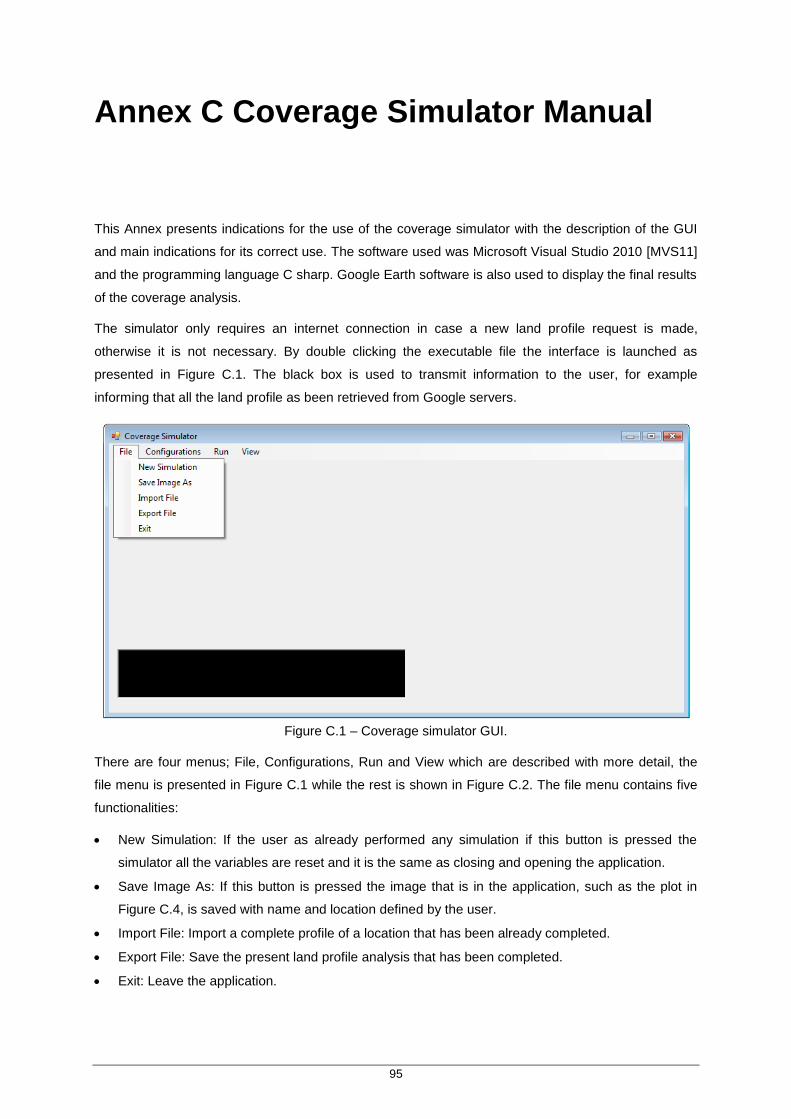
95
Annex C Coverage Simulator Manual
Annex C - Coverage Simulator Manual
This Annex presents indications for the use of the coverage simulator with the description of the GUI
and main indications for its correct use. The software used was Microsoft Visual Studio 2010 [MVS11]
and the programming language C sharp. Google Earth software is also used to display the final results
of the coverage analysis.
The simulator only requires an internet connection in case a new land profile request is made,
otherwise it is not necessary. By double clicking the executable file the interface is launched as
presented in Figure C.1. The black box is used to transmit information to the user, for example
informing that all the land profile as been retrieved from Google servers.
Figure C.1 – Coverage simulator GUI.
There are four menus; File, Configurations, Run and View which are described with more detail, the
file menu is presented in Figure C.1 while the rest is shown in Figure C.2. The file menu contains five
functionalities:
New Simulation: If the user as already performed any simulation if this button is pressed the
simulator all the variables are reset and it is the same as closing and opening the application.
Save Image As: If this button is pressed the image that is in the application, such as the plot in
Figure C.4, is saved with name and location defined by the user.
Import File: Import a complete profile of a location that has been already completed.
Export File: Save the present land profile analysis that has been completed.
Exit: Leave the application.
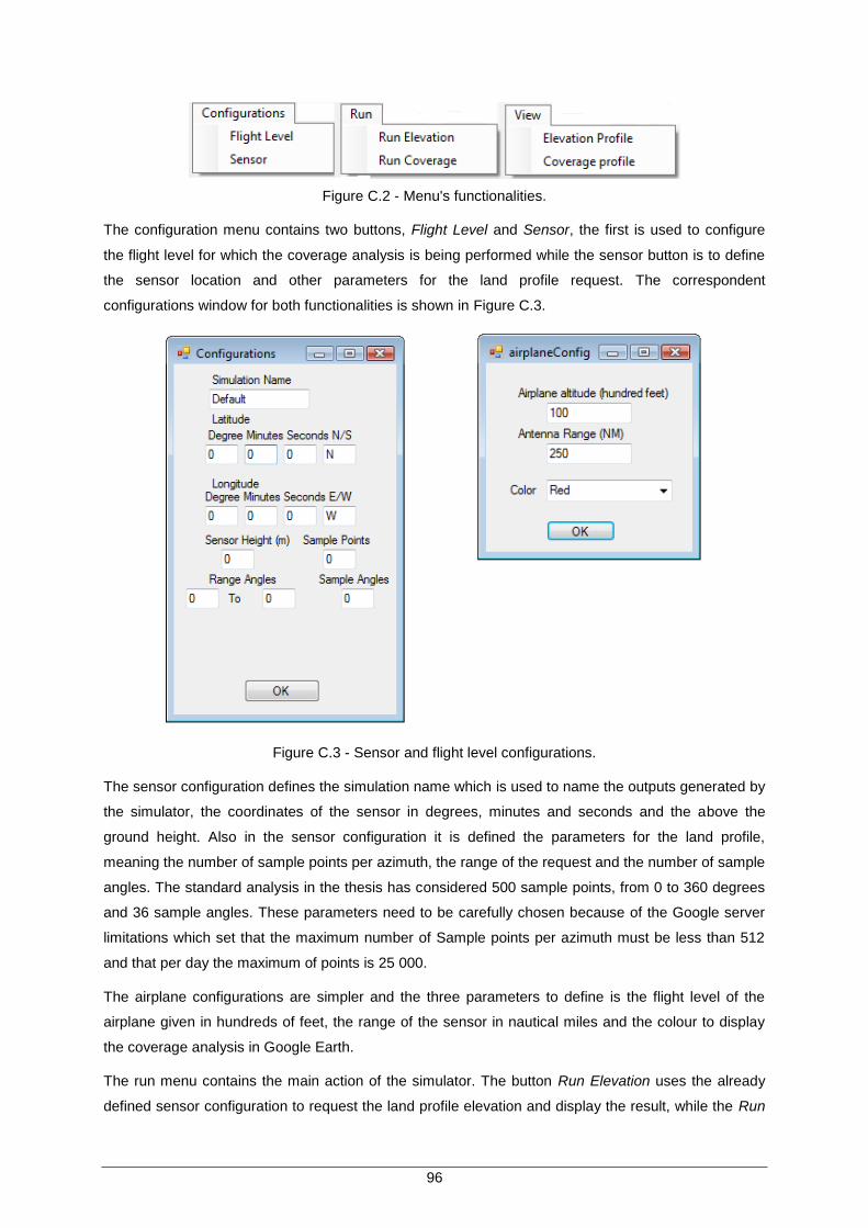
96
Figure C.2 - Menu's functionalities.
The configuration menu contains two buttons, Flight Level and Sensor, the first is used to configure
the flight level for which the coverage analysis is being performed while the sensor button is to define
the sensor location and other parameters for the land profile request. The correspondent
configurations window for both functionalities is shown in Figure C.3.
Figure C.3 - Sensor and flight level configurations.
The sensor configuration defines the simulation name which is used to name the outputs generated by
the simulator, the coordinates of the sensor in degrees, minutes and seconds and the above the
ground height. Also in the sensor configuration it is defined the parameters for the land profile,
meaning the number of sample points per azimuth, the range of the request and the number of sample
angles. The standard analysis in the thesis has considered 500 sample points, from 0 to 360 degrees
and 36 sample angles. These parameters need to be carefully chosen because of the Google server
limitations which set that the maximum number of Sample points per azimuth must be less than 512
and that per day the maximum of points is 25 000.
The airplane configurations are simpler and the three parameters to define is the flight level of the
airplane given in hundreds of feet, the range of the sensor in nautical miles and the colour to display
the coverage analysis in Google Earth.
The run menu contains the main action of the simulator. The button Run Elevation uses the already
defined sensor configuration to request the land profile elevation and display the result, while the Run

97
Coverage uses the elevation profile elevation to get the final global coverage. Finally, the view menu
allows to change between the view of a given azimuth profile, Figure C.4 , or the coverage line of the
same profile, Figure C.6.
This summarised a walkthrough of the functionalities available in the simulator for better
understanding of the sequence of operations to perform in the simulator. The main goal of the
simulator is first to have a land profile analysis and only then get the global coverage.
After starting the program, to get a land profile of a given sensor and to display it in the application
there are two possible ways:
Import a pre-saved file with a land profile and then click in the view elevation profile button. The
text box will display “File successfully imported!” in case of success.
Configure the sensors in the configurations menu and then run the elevation profile; the elevation
profile of the first azimuth is automatically displayed. The text box will display “All points
successfully downloaded!” in case of success.
Having the elevation profile displayed, Figure C.4, it is possible to navigate between azimuth by
pressing the Prev and Next button and also to plot the height correction and remove it with the
correspondent buttons. Pressing the height correction button, Figure C.5 is presented. In the previous
situation it is also possible see the coverage line for the given azimuth by pressing view coverage
profile and it is displayed as shown in Figure C.6.
Figure C.4 - Display of the land elevation profile.
It is in this situation, after the land profile request that there is enough information to export a file and
store the information for future use. By pressing the export file in the file menu it is created a file with
the simulation information whose name is the conjugation of “Output_” with the simulation name. The
structure of the file is; simulation name (enter), sensor‟s latitude (enter), sensor‟s longitude (enter),
sensor‟s height (enter), number of azimuths in the file followed by a blank line. After the blank line
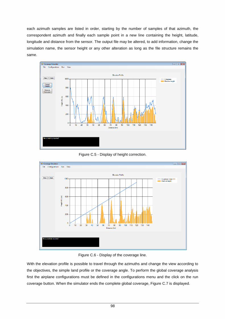
98
each azimuth samples are listed in order, starting by the number of samples of that azimuth, the
correspondent azimuth and finally each sample point in a new line containing the height, latitude,
longitude and distance from the sensor. The output file may be altered, to add information, change the
simulation name, the sensor height or any other alteration as long as the file structure remains the
same.
Figure C.5 - Display of height correction.
Figure C.6 - Display of the coverage line.
With the elevation profile is possible to travel through the azimuths and change the view according to
the objectives, the simple land profile or the coverage angle. To perform the global coverage analysis
first the airplane configurations must be defined in the configurations menu and the click on the run
coverage button. When the simulator ends the complete global coverage, Figure C.7 is displayed.

99
Figure C.7 - Global coverage display.
Simultaneously with the coverage diagram a (*.kml) file with the name of the simulation is created in
the same folder as the executable file. The kml file can be opened using Google Earth software and
an example of the image displayed is shown in Figure C.8.
Figure C.8 - Google Earth coverage display.
It should be noticed that the development of the simulator would not be possible without the worldwide
contribution of Google in geographical systems technology, more specifically in the elevation data, the
Google Earth software and the open information from Google codes. I am hereby showing my
appreciation to their work.
This Annex presented a brief manual to use the coverage simulator whose source code and
executable file is supplied together with the thesis.

101
Annex D Lisbon sensors coverage
Annex D - Lisbon Sensors Coverage
Figure D.1 - Overall sensor‟s coverage Lisbon LAM (extracted from [Sns09c]).
Figure D.2 - Individual coverage of sensor RU1 to RU6 (extracted from [Sns09c]).
Figure D.3 - Individual coverage of sensor RU7 to RU12 (extracted from [Sns09c]).
Figure D.4 - Individual coverage sensor RU13 and RU14 (extracted from [Sns09c]).
Figure D.5 - Arrabida sensor coverage (obtained from [NAV11]).
Figure D.6 - Caparica sensor coverage (obtained from [NAV11]).
Figure D.7 - Espichel sensor coverage (obtained from [NAV11]).
Figure D.8 - Fanhões sensor coverage (obtained from [NAV11]).
Figure D.9 - Montargil sensor coverage (obtained from [NAV11]).
Figure D.10 - Montejunto sensor coverage (obtained from [NAV11]).
Figure D.11 - TAR sensor coverage (obtained from [NAV11]).


103
Annex E North sensors coverage
Annex E - North Sensors Coverage
Figure E.1 – Sensor 1 and sensor 2 individual coverage.
Figure E.2 – Sensor 3 and sensor 4 individual coverage.
Figure E.3 – Sensor 5 and sensor 6 individual coverage.
Figure E.4 – Sensor 7 and sensor 8 individual coverage.
Figure E.5 – Sensor 9 and sensor 10 individual coverage.
Figure E.6 – Sensor 11 and sensor 12 individual coverage.
Figure E.7 – Sensor 13 and sensor 14 individual coverage.
Figure E.8 - Bragança and Bragança VOR individual coverage.
Figure E.9 - Ovar Tacan and Porto Locator individual coverage.
Figure E.10 - Porto NDB and Viseu Individual coverage.


105
Annex F – Global Coverage Study
Annex F – Global Coverage Study
Figure F.1 – First proposal global coverage.
Figure F.2 - Second proposal global coverage.
Figure F.3 - Third proposal global coverage.
Figure F.4 - Fourth proposal global coverage.

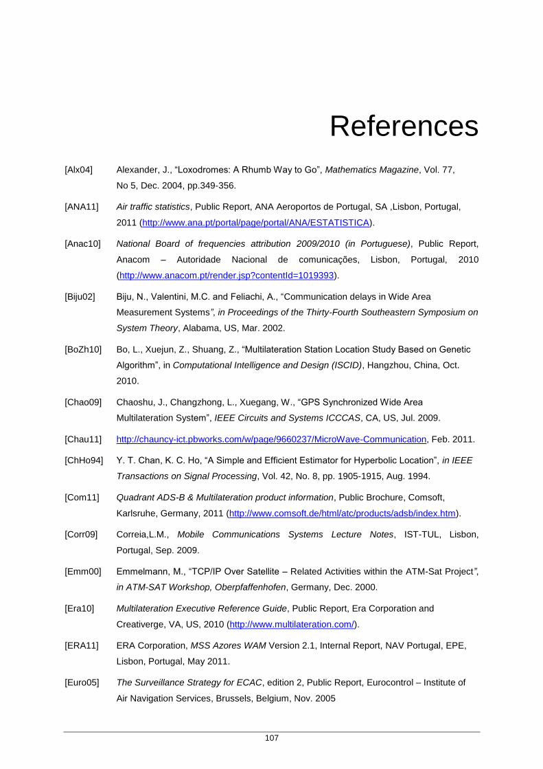
107
References
References
[Alx04] Alexander, J., “Loxodromes: A Rhumb Way to Go”, Mathematics Magazine, Vol. 77,
No 5, Dec. 2004, pp.349-356.
[ANA11] Air traffic statistics, Public Report, ANA Aeroportos de Portugal, SA ,Lisbon, Portugal,
2011 (http://www.ana.pt/portal/page/portal/ANA/ESTATISTICA).
[Anac10] National Board of frequencies attribution 2009/2010 (in Portuguese), Public Report,
Anacom – Autoridade Nacional de comunicações, Lisbon, Portugal, 2010
(http://www.anacom.pt/render.jsp?contentId=1019393).
[Biju02] Biju, N., Valentini, M.C. and Feliachi, A., “Communication delays in Wide Area
Measurement Systems”, in Proceedings of the Thirty-Fourth Southeastern Symposium on
System Theory, Alabama, US, Mar. 2002.
[BoZh10] Bo, L., Xuejun, Z., Shuang, Z., “Multilateration Station Location Study Based on Genetic
Algorithm”, in Computational Intelligence and Design (ISCID), Hangzhou, China, Oct.
2010.
[Chao09] Chaoshu, J., Changzhong, L., Xuegang, W., “GPS Synchronized Wide Area
Multilateration System”, IEEE Circuits and Systems ICCCAS, CA, US, Jul. 2009.
[Chau11] http://chauncy-ict.pbworks.com/w/page/9660237/MicroWave-Communication, Feb. 2011.
[ChHo94] Y. T. Chan, K. C. Ho, “A Simple and Efficient Estimator for Hyperbolic Location”, in IEEE
Transactions on Signal Processing, Vol. 42, No. 8, pp. 1905-1915, Aug. 1994.
[Com11] Quadrant ADS-B & Multilateration product information, Public Brochure, Comsoft,
Karlsruhe, Germany, 2011 (http://www.comsoft.de/html/atc/products/adsb/index.htm).
[Corr09] Correia,L.M., Mobile Communications Systems Lecture Notes, IST-TUL, Lisbon,
Portugal, Sep. 2009.
[Emm00] Emmelmann, M., “TCP/IP Over Satellite – Related Activities within the ATM-Sat Project”,
in ATM-SAT Workshop, Oberpfaffenhofen, Germany, Dec. 2000.
[Era10] Multilateration Executive Reference Guide, Public Report, Era Corporation and
Creativerge, VA, US, 2010 (http://www.multilateration.com/).
[ERA11] ERA Corporation, MSS Azores WAM Version 2.1, Internal Report, NAV Portugal, EPE,
Lisbon, Portugal, May 2011.
[Euro05] The Surveillance Strategy for ECAC, edition 2, Public Report, Eurocontrol – Institute of
Air Navigation Services, Brussels, Belgium, Nov. 2005

108
(http://www.eurocontrol.int/surveillance/gallery/content/public/documents/strategy.pdf).
[Euro08] Eurocontrol – Institute of Air Navigation Services, SUR/ADSB MLAT Courses, Workshops
and Seminars Material, Kirchberg, Luxemburg, Jan. 2008.
[Euro09] Wide Area Multilateration – A Surveillance Technique That Is Ready For Use, Press
Release, Eurocontrol – Institute of Air Navigation Services, Brussels, Belgium, 2009
(http://www.eurocontrol.int/press-releases/wide-area-multilateration-%E2%80%93-
surveillance-technique-ready-use).
[FIA08] Gilmore, M., Understanding OM1, OM2, OM3, OS1, OS2 and more!, Fibreoptic Industry
Association, Hertfordshire, UK, 2008
(https://learningnetwork.cisco.com/servlet/JiveServlet/previewBody/3791-102-1-
10509/Understanding%20OM1,OM2,OM3,%20OS1,OS2%20Fibre.pdf).
[FIA10] Modified Bandwidth Specifications For OM3 and OM4, White Paper, Fibreoptic Industry
Association, Hertfordshire, UK, 2010 (http://www.fia-online.co.uk/pdf/Whites/wp0110.pdf).
[Fig02] Figanier, J., Propagation Aspects in the Atmosphere (in Portuguese), IST-TUL press,
edition by Fernandes, C.A., Lisbon, Portugal, 2002.
[Fols08] Choosing the Right Multimode Fibre for Data Communications, White Paper, Fols, Sep.
2008 (http://fols.org/fols_library/white_papers/documents/mmfibrewhitepaper.pdf).
[Go11a] KML documentation, Documentation, Google, CA, US, 2011
(http://code.google.com/intl/pt/apis/kml/documentation/).
[Go11b] The Google Elevation API, Documentation, Google, CA, US, 2011,
(http://code.google.com/intl/pt/apis/maps/documentation/elevation/).
[Go11c] Google Maps API for .NET, Documentation, Google, CA, US, 2011,
(http://code.google.com/p/gmaps-api-net/).
[IGP10] Oficial administrative letter of Portugal (in portuguese), Public Report, Instituto Geográfico
Português, Lisbon, Portugal, 2010
(http://www.igeo.pt/produtos/cadastro/caop/inicial.htm).
[ISat11] http://www.intelsat.com/resources/satellite-basics, Feb. 2011.
[ITU03] ITU-R, The radio refractive index: its formula and refractivity data, Recommendation ITU-
R P.453, V.9, 2003 (http://www.itu.int/rec/R-REC-P.453/en).
[ITU09] ITU-R, Propagation data and prediction methods requires for the design of terrestrial line-
of-sight systems, Recommendation ITU-R P.530, V.13, 2009 (http://www.itu.int/rec/R-
REC-P.530/en).
[ITUT09] ITU-T, Transmission characteristics of optical components and subsystems,
Recommendation ITU-T G.671, Jan. 2009 (http://www.itu.int/itu-
t/recommendations/rec.aspx?id=9645).
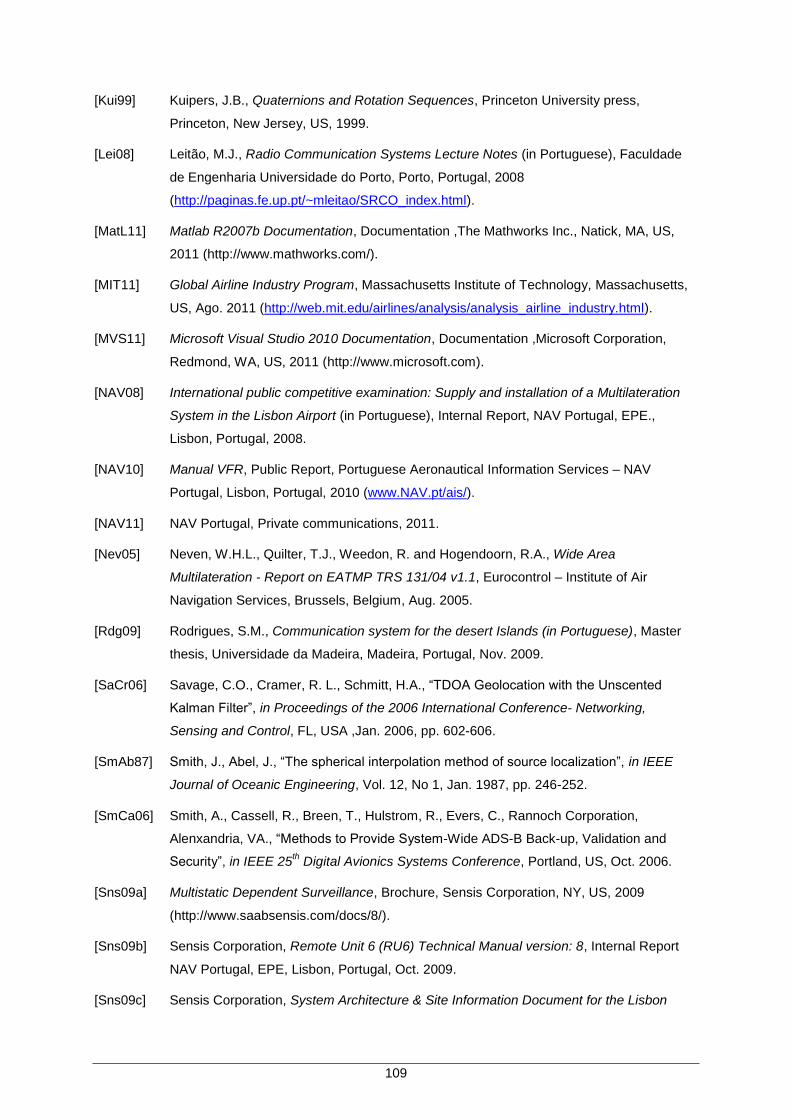
109
[Kui99] Kuipers, J.B., Quaternions and Rotation Sequences, Princeton University press,
Princeton, New Jersey, US, 1999.
[Lei08] Leitão, M.J., Radio Communication Systems Lecture Notes (in Portuguese), Faculdade
de Engenharia Universidade do Porto, Porto, Portugal, 2008
(http://paginas.fe.up.pt/~mleitao/SRCO_index.html).
[MatL11] Matlab R2007b Documentation, Documentation ,The Mathworks Inc., Natick, MA, US,
2011 (http://www.mathworks.com/).
[MIT11] Global Airline Industry Program, Massachusetts Institute of Technology, Massachusetts,
US, Ago. 2011 (http://web.mit.edu/airlines/analysis/analysis_airline_industry.html).
[MVS11] Microsoft Visual Studio 2010 Documentation, Documentation ,Microsoft Corporation,
Redmond, WA, US, 2011 (http://www.microsoft.com).
[NAV08] International public competitive examination: Supply and installation of a Multilateration
System in the Lisbon Airport (in Portuguese), Internal Report, NAV Portugal, EPE.,
Lisbon, Portugal, 2008.
[NAV10] Manual VFR, Public Report, Portuguese Aeronautical Information Services – NAV
Portugal, Lisbon, Portugal, 2010 (www.NAV.pt/ais/).
[NAV11] NAV Portugal, Private communications, 2011.
[Nev05] Neven, W.H.L., Quilter, T.J., Weedon, R. and Hogendoorn, R.A., Wide Area
Multilateration - Report on EATMP TRS 131/04 v1.1, Eurocontrol – Institute of Air
Navigation Services, Brussels, Belgium, Aug. 2005.
[Rdg09] Rodrigues, S.M., Communication system for the desert Islands (in Portuguese), Master
thesis, Universidade da Madeira, Madeira, Portugal, Nov. 2009.
[SaCr06] Savage, C.O., Cramer, R. L., Schmitt, H.A., “TDOA Geolocation with the Unscented
Kalman Filter”, in Proceedings of the 2006 International Conference- Networking,
Sensing and Control, FL, USA ,Jan. 2006, pp. 602-606.
[SmAb87] Smith, J., Abel, J., “The spherical interpolation method of source localization”, in IEEE
Journal of Oceanic Engineering, Vol. 12, No 1, Jan. 1987, pp. 246-252.
[SmCa06] Smith, A., Cassell, R., Breen, T., Hulstrom, R., Evers, C., Rannoch Corporation,
Alenxandria, VA., “Methods to Provide System-Wide ADS-B Back-up, Validation and
Security”, in IEEE 25th Digital Avionics Systems Conference, Portland, US, Oct. 2006.
[Sns09a] Multistatic Dependent Surveillance, Brochure, Sensis Corporation, NY, US, 2009
(http://www.saabsensis.com/docs/8/).
[Sns09b] Sensis Corporation, Remote Unit 6 (RU6) Technical Manual version: 8, Internal Report
NAV Portugal, EPE, Lisbon, Portugal, Oct. 2009.
[Sns09c] Sensis Corporation, System Architecture & Site Information Document for the Lisbon

110
Multistatic Dependent Surveillance (MDS) System Version 3, Internal Report, NAV
Portugal, EPE., Lisbon, Portugal, Dec. 2009.
[Swp11] http://sonkusare.wordpress.com/2010/12/30/satellite-communication/, Feb.2011.