assessing the spatial accessibility of microfinance in ...€¦ · analyzing any spatial...
TRANSCRIPT

JOURNAL OF REGIONAL SCIENCE, VOL. 00, NO. 0, 2015, pp. 1–29
ASSESSING THE SPATIAL ACCESSIBILITY OF MICROFINANCE INNORTHERN BANGLADESH: A GIS ANALYSIS*
Akib KhanJames P. Grant School of Public Health, BRAC University, Mohakhali, Dhaka 1212, Bangladesh.E-mail: [email protected]
Atonu RabbaniDepartment of Economics, University of Dhaka, Nilkhet Road, Dhaka 1000, Bangladesh.E-mail: [email protected]
ABSTRACT. This paper attempts to understand and operationalize the notion of spatial accessibility(SA) in the context of microfinance. Using geographic information system (GIS) data from northernBangladesh, we have generated a kernel-smoothed map and found remarkable spatial variation inaccess to microcredit. Results suggest that areas isolated from physical infrastructure, administrativeestablishments, and prone to ecological shocks, exhibit lower degree of SA. Moreover, using an instru-mental variable framework, we found that SA has a significant positive impact on household’s decisionto borrow and on the number of loans: one standard deviation higher SA is associated with a rise inparticipation probability and average number of microloans by, at least, 3.5 percentage points and 16percent, respectively.
1. INTRODUCTION
A very diverse and interrelated set of variables may influence the behavior of microfi-nance institutions (MFIs) (e.g., location choice, design of financial instruments, profitabil-ity, operational sustainability, and personnel productivity) and that of their prospectiveclients (e.g., formal, semiformal, or informal borrowing, crisis coping, repayment strategy,and horizontal or vertical mobility in the socioeconomic hierarchy). Typically, the focus ofthe researchers, to date, has been on specifying, analyzing, and evaluating the influence offactors that are, by nature, economic, sociocultural, structural, or demographic (Hossain,1988; Rahman, 1996; Zeller et al., 2001; Navajas et al., 2002; Fruttero and Gauri, 2005).
In this paper, we attempt to emphasize the geospatial aspects of microfinance by uti-lizing a geographic information system (GIS), particularly scrutinizing the supply side.Geographical features can have important implications for the functioning of the microfi-nance market in many ways. For instance, the spatial status of both the household itselfand the service providers (i.e., the MFIs) can substantially affect the borrowing behaviorand effective participation of a household in the formal credit market. Distance to branch
*The authors would like to thank JRS Co-Editor Steven Brakman and two anonymous referees formany useful comments and suggestions. Special thanks also go to M. Shahe Emran and the seminar par-ticipants at the Economic Research Group (Dhaka, Bangladesh) for helpful suggestions and instructionsthat have benefited the authors a lot. The authors would also like to acknowledge the Institute of Microfi-nance (InM) for allowing the authors to use the data used in this paper. The data were collected as a partof an evaluation project for Programmed Initiatives for Monga Eradication (PRIME). The funding camefrom the Department for International Development’s (DfID) Promoting Financial Services for PovertyReduction Programme (PROSPER). The research assistance from Mehadi Hasan and Bakhtiar Sohag isalso highly appreciated.
Received: May 2013; revised: January 2015; accepted: January 2015.
C© 2015 Wiley Periodicals, Inc. DOI: 10.1111/jors.12196
1
2 JOURNAL OF REGIONAL SCIENCE, VOL. 00, NO. 0, 2015
and costs of communication are likely to play vital roles in hindering active participationand hence are issues of great significance because extending outreach to the hard-to-reachpopulation has received much attention lately (Cull, Demirguc-Kunt, and Morduch, 2009;Hermes, Lensink, and Meesters, 2011). Therefore, understanding the roles of geographicaccess to MFI services should provide useful guidance on how to advance this industryeven further and expand coverage in the underserved areas. In this paper, we attemptto understand the underlying rationale and evaluate the consequences of the geospatialfeatures of MFI activities.
Prior studies have already attempted to address the association between the useand access to credit and the spatial distribution of financial services availability (asmeasured, for example, by the number of bank branches or ATMs per 1,000 km2; Beck,Demirguc-Kunt, and Peria, 2007; World Bank, 2008). These studies have mostly relied onthe distribution of access across countries by primarily focusing on the access to formalcredit only. In this paper, we explicitly model within-country/region spatial heterogeneityin access to credit. Our study attempts to fulfill the dual objective of complementingprior studies by exploiting the individual household-level variation in access to financewith the aid of better indicators of spatial access and improving on their exploration ofthe association between access and utilization by explicitly addressing the econometricproblem of endogeneity. Furthermore, in rural Bangladesh, it is more reasonable to lookat the microfinance sector that has become the dominant financial intermediary in therural area over the last three decades.
GIS has undeniably been an indispensable, cost-effective, and accessible tool forthe researchers (of diverse background) as well as the policymakers in discovering andanalyzing any spatial phenomenon. For example, it has become a widespread practice touse hospital and health clinic locations to both estimate the geographic accessibility ofhealth care and evaluate its impact on the rate of utilization through spatial analysis(Luo and Wang, 2003; McLafferty and Grady, 2004). Studies have also been carried outon using locations of criminal activities to pin down crime hotspots, thus facilitating themobilization of law enforcing efforts (McLafferty, Williamson, and McGuire, 1999).
In the present study, we first draw from prior theoretical and empirical studies onspatial accessibility (SA) and develop a theoretical structure to conceptualize the notionof geographical accessibility in the context of microfinance. Based on this framework,we generate continuous accessibility surfaces (or maps) for the districts of Kurigram andLalmonirhat (from northern Bangladesh) incorporating all active MFI branches by meansof kernel interpolation—a measure frequently used to estimate spatial access. We also aimto isolate the spatial factors that might explain the observed diffusion of microcredit access(as measured by SA). We find that geographical detachment from physical infrastructureand administrative centers and exposure of the households to potential negative ecologicalshocks significantly reduce the spatial access to microfinancial services. Moreover, theaccessibility estimates are found to be robustly associated with microfinance participation.
Hereafter, the paper will proceed as follows: Section 2 will provide a discussion ofdefinitional issues, whereas Sections 3, 4, and 5 will deal with issues regarding measure-ment, approach, and data. Interpretation of geointerpolated maps and empirical findingsare presented in Section 6. Under Section 7, we discuss briefly the policy relevance andshortcomings of the study. Finally, in Section 8, the paper concludes by making some finalcomments and highlighting the potentials of additional investigative studies.
2. SA: SOME DEFINITIONAL ISSUES
Despite often being used interchangeably, availability and accessibility representtwo different spatial concepts. Availability refers to the number of service providers to be
C© 2015 Wiley Periodicals, Inc.
KHAN AND RABBANI: SPATIAL ACCESSIBILITY OF MICROFINANCE IN NORTHERN BANGLADESH 3
taken into consideration by an individual while making a choice, whereas accessibility canbe viewed as the spatial connectivity between potential consumers and existing servicepoints (often measured in terms of commuting constraints such as distance or time)(Guagliardo, 2004).1 However, in the literature of social sciences and geography, thesetwo aspects have often been integrated into one single concept of “spatial accessibility”(SA) (Khan and Bhardwaj, 1994).
Each field of study and/or area of application (e.g., healthcare, education, and publictransport system), taking into account all of its distinctive attributes, has developed a wideand diverse range of approaches to successfully conceptualize spatial access (Khan andBhardwaj, 1994). Studies that have been undertaken thus far, in different fields, suggestthat availability and accessibility may rely substantially on geographic features such asdistance and travel time. For example, in the setting of healthcare, the transportation costsfaced by a healthcare seeker work as one of the primary determinants of spatial access and,therefore, utilization (Goodman et al., 1997). The case is almost identical for geographicaccess to educational services where the availability of an educational institution has beenpostulated as a decreasing function of distance for prospective students (Binita, 2010).
As far as the functioning of microfinance market is concerned, the relative impor-tance of provider (e.g., an MFI) and potential client (e.g., a poor rural household) locationsis somewhat different. MFIs reach out to potential clients by placing the branches strate-gically (Salim, 2013). Using these branches as hubs, credit or loan officers form clientgroups in the neighborhoods of poor households and make frequent visits to establish aneffective network of communication with the customers through these community groups(Armendariz and Morduch, 2005). It is important for an MFI to reach out to a potentialclient base that is poor and geographically more detached. However, this objective is con-strained by the concern for the sustainability of MFIs. This is often synonymous with costminimization. MFIs’ location choice often depends on these conflicting dual objectives, andthis paper intends to contribute to the understanding of the location decision of the MFIsin the two districts of Bangladesh where historically, lack of communication facilities hascontributed to economic underdevelopment and destitute (Mahmud, 2011).
Because of the associations it has with the costs of transportation and prevalenceof asymmetric information, the “distance” factor in the context of banking has receivedgreater attention in the academic domain in the recent past (Alessandrini, Fratianni,and Zazzaro, 2009). As Pedrosa and Do (2011) have pointed out, the costs of deliveringfinancial services to the borrowers and monitoring microfinance beneficiaries who aregeographically scattered in hard-to-reach rural areas can have a significant impact onthe “profitability” of the MFIs. MFIs may limit operation to areas with certain spatialqualities (better accessibility with lower ecological vulnerability and natural disasters) orimpose more demanding eligibility requirements (e.g., compulsory savings, more frequentrepayments resulting in higher rate of rejection) and/or raise interest rates. Besidesthat, MFIs may encounter riskier demand from the hard-to-reach client base which,due to spatial isolation, presumably suffers from lower human development, productioninstability, and susceptibility to negative economic and noneconomic shocks. Hence, evenif MFIs were able to reduce costs on the intensive margin by enhancing monitoringcapability, the distance-induced rise in extensive margin expenses would still remain asource of concern.
Pedrosa and Do (2011) tested some of these hypotheses about the impact of distanceusing data from Niger, where distant borrowers were observed to be economically more
1Note that the notion of “accessibility” is concerned with the “potential” and not the “realized” accessto the services being provided. Throughout the text, henceforth, whenever brought up, the term accessibilitywill be used to signify the prospects of implementation (irrespective of the context).
C© 2015 Wiley Periodicals, Inc.

4 JOURNAL OF REGIONAL SCIENCE, VOL. 00, NO. 0, 2015
vulnerable and worse off in terms of getting access to financial services. The results alsosuggest that an increase in distance implies rising costs (both transaction and monitoring)for the MFIs, which has been, to some extent, shifted to the borrowers in the form of higherinterest rates and additional constraints. This also leads to the exclusion of marginal bor-rowers (who are observed to move upward in the income distribution as distance increases)from the formal and/or quasi-formal rural credit market. This then implies both: (a) thelikelihood of being provided with microcredit diminishes with spatial detachment from theproviders and (b) MFIs’ inclination toward serving the relatively less impoverished pop-ulation increases with geographic distance. Empirical evidence where the rise in agencycosts caused by the spatial segregation of the client and MFI makes the credit marketmore prone to moral hazard also exist (Presbitero and Rabellotti, 2014). The existing stockof literature, however, offers mixed evidence on the relationship between spatial gap andthe odds of reimbursement. Oke, Adeyemo, and Agbonlahor (2007) found distance to beinversely related to the repayment rate in Nigeria. On the other hand, Roslan and Karim(2009) failed to find any such association for the Malaysian microcredit market.
The existing literature then leads us to deduce that, ceteris paribus, the further away(geographically speaking) one is from an MFI, the lower will be the likelihood of his/herbeing a user of its financial services; spatial access to microfinance services diminisheswith distance. To summarize, in order to obtain adequacy in composition, an SA indexshould take into consideration the following: (a) inclusion of all potentially accessibleservice points (i.e., branch offices) and (b) discounting the branches according to theirgeographical location.2
3. MEASURING SA USING KERNEL DENSITY ESTIMATION (KDE)
Among the potential measures of SA, it is most common to use distance to the nearestservice provider because of its intuitiveness and ease of interpretability. However, distanceto the nearest service provider ignores the households’ capacity to access other competingMFIs. Hence, in areas where multiple providers exist and operate in the immediatevicinity of a household (a valid possibility in the case of microfinance), the distance to thenearest MFI branch may be a narrow and even a misleading estimate of accessibility. Onthe other hand, “provider-to-population ratios” (e.g., number of MFIs per 100,000 people)and “simple density” (e.g., number of MFI branches per square kilometer; both used byBeck et al., 2007, but for the set of formal financial institutions only), despite beingable to include all relevant branch offices, ignore the intraregion variability in providerpenetration, one of the key aspects we aim to explore and utilize. In other words, theyfail to discount MFI branches with increasing distance that, as has been argued above,is critical to the estimation of microfinance SA. Though “average distance to providers”overcomes this to some extent, it is inadequate in capturing the intensity of MFI activities(for example, the number of MFI branches operating could be very dissimilar despite thesame “average distance” figure).
2Also, ceteris paribus, the higher the density of potential clients surrounding an individual, thegreater the competition he/she will possibly face in terms of ensuring access. But one should note thattwo opposing forces are in effect here in terms of relevant population density; the more remote a locationis, the lower the (general) population density might be but the higher the proportion of potential clientssince that location would be more likely less developed. As a result, the potential client density may bemore/less equalized across the study area. Our SA estimates, which are based on the supply side onlydue to unavailability of data on the demand side, therefore, may not be that much biased. The regressionresults, as discussed in Section 6, which control for union-level population density, further lend support tothis conjecture.
C© 2015 Wiley Periodicals, Inc.
KHAN AND RABBANI: SPATIAL ACCESSIBILITY OF MICROFINANCE IN NORTHERN BANGLADESH 5
Apart from the gravity model, only KDE addresses the two basic issues regardingthe measurement of geographical accessibility while being conceptually easier to graspand rationalize than the gravity measure (Guagliardo, 2004; Hass, 2009). But the spatialseparation of the provider and the client has to be measured in Euclidean or straight-line distance, which may lead to under/overestimation of travel impedance. However,in contrast to any rural setting (which, in general, has been the focus of microfinance),the problem is presumably more acute in urban areas due to its complex transportationnetwork resulting from significantly higher density of settlements.
While KDE (in the context of generating smooth geospatial surface) has a few draw-backs, we chose the current method (over, say, similar methods such as gravity model)for the following reasons. First, there already exists an established and consistent seriesof literature that have critically analyzed the theoretical and applied issues concerningkernel interpolation in diverse market environments (Luo and Wang, 2003; Guagliardo,2004; McLafferty and Grady, 2004; Yang, Goerge, and Mullner, 2006; Gibin, Longley, andAtkinson, 2007; Spencer and Angeles, 2007; Xie and Yan, 2008; Binita, 2010; Schuur-man, Berube, and Crooks, 2010). These applications of KDE can serve as useful referencepoints, thus enabling us to effectively adopt kernel smoothing to measure spatial accessof microfinance. Second, recent progress in the frontier of GIS software development hasremarkably facilitated the computation of kernel density in terms of ease and accuracy. Ina nutshell, then, KDE, as an SA measure, is frequently applied, more intuitive in natureand easily estimable.3
4. DATA
Lalmonirhat and Kurigram are two of the northern districts of Bangladesh thathave received considerable attention from academicians, policymakers, and developmentpractitioners (Hossain et al., 2005; Zohir et al., 2007; Mahmud, 2011; Mobarak, 2011).4
This region is particularly characterized by its distinct geographic attributes (a river-ine, low-lying flat plane prone to floods and river erosion) and comparatively low levelsof human development (Zug, 2006). Extreme climate condition, coupled with frequentnatural calamities (mainly caused by the abundance of rivers) and underdeveloped phys-ical infrastructure, has proved to be one of the major impediments to the socioeconomicprogress of the bulk of its population. Often being a victim of pronounced periodic fluc-tuations in the availability of income-earning activities, especially during the season ofmonga,5 the majority of its households struggle to maintain a consistent standard ofliving.
To facilitate these households with access to semiformal and formal financial ser-vices, many MFIs have expanded their operation to these two districts. In 2010 (the yearof data collection), there were 224 and 165 MFI branches in Kurigram and Lalmonirhat,
3Our estimation of kernel density, however, as would also be encountered in the case of the gravitymodel, will suffer from the absence of data on the demand side of the market (i.e., potential credit clients).The data set is also deficient in containing information on the capacity of all the MFIs operating withinthe study area. As a result, we will have to adopt KDE exclusively based on a rather narrowly representedsupply side of the microfinance market.
4The northwestern parts of Bangladesh have typically been more impoverished (BBS, 2006). Therecent survey also reveals that the Rangpur division (which Kurigram and Lalmonirhat are part of)remained the second highest recipient of social safety net programs (Bangladesh Bureau of Statistics,2011).
5A word from local dialect referring to the sudden degradation of the living standard due to the lackof entitlement to basic food and nonfood components of consumption, basically caused by an intense dearthof jobs, typically experienced in the off-crop seasons.
C© 2015 Wiley Periodicals, Inc.
6 JOURNAL OF REGIONAL SCIENCE, VOL. 00, NO. 0, 2015
respectively. GIS data collection was mainly operationalized as a pilot project supple-mentary to the core Programmed Initiatives for Monga Eradication (PRIME) third roundstudy.6 The project’s primary focus was to collect location information of all active MFIbranches, along with roads, administrative headquarters at union, thana/upazila, and dis-trict levels (appearing in an ascending order within the public administration hierarchy),and major topographical attributes such as rivers and char-lands7 within our study area.We also have GIS data on the geographic location of a set of cluster-sampled ultra-poorhouseholds (1,974 of them: 885 from Lalmonirhat and 1,089 from Kurigram; ultra-poorhouseholds are defined as having less than 50 decimals of cultivable land, earning lessthan 1,500 taka (US$22) per month, and working mostly as wage laborers) (see Figure 1for a selective mapping of the GIS information collected). Along with the GIS information,we also made use of a unique data set containing information on different economic andnoneconomic aspects of the same set of households.
5. METHODOLOGY
Given the discrete data points with spatially extensive attributes, KDE generatesan interpolated surface that is continuous in nature and unconstrained by geopoliticalboundaries (Spencer and Angeles, 2007). In the context of microfinance, this amountsto the generation of a continuous accessibility map given the location data of MFIs. Theapplication of KDE results in a raster data set (composed of equally sized cells) whereeach cell is ascribed an interpolated SA value (Longley et al., 2005). The estimationprocedure, first of all, assigns a cone or kernel to each of the MFI branches. The kernelis placed upon such that its center coincides with the host branch office location on themap surface. A provider’s aggregate capacity is represented by the associated cone’svolume that, if not specified, is typically assumed to be one (which is the case here). Asstated before, the allocation of capacity administered by an MFI branch is indicative ofthe associated degree of accessibility. The cones are modeled via a kernel function, whichdistributes an MFI’s service capacity as a strictly decreasing function of geographicaldistance; i.e., the further away a cell (underlying the cone) is from its center (i.e., thebranch office), the smaller the value of capacity it will be assigned (for reasons discussedin detail in Section 2). KDE, therefore, accounts for the “distance decay effect,” one ofthe fundamentals characterizing the SA of microfinance. If summed up, the densityvalues of all the cells enclosed by a cone will be equal to the total capacity of the relevantbranch. Since the provider cones are often found to be overlapping as a consequenceof intersecting service areas of multiple providers, the accessibility value for a cell isfinalized by adding up all the kernel surfaces that overlay the cell center.
Put simply, the surface generated by KDE is in effect tantamount to a 3-D histogramof MFI branch presence. But unlike a standard histogram where each observation istreated as a discrete data point, here an MFI branch’s presence (which contributes to the“frequency” calculation of the associated location) is distributed as a cone over its potentialservice area. Upon vertical summation of all these cones, the resultant surface merelyrepresents the density of MFI branches across the study area. The MFIs, as explainedearlier (see Section 2), operate through their branches. The height of the surface at any
6PRIME is a DfID funded project that includes providing microcredit and ancillary services such ashealth treatment and training to the ultra-poor households in the northwestern part of Bangladesh. Theproject started in 2006 and is scheduled to end in 2014.
7Char is a local word to describe a strip of sandy land rising out of the bed of a river above waterlevel.
C© 2015 Wiley Periodicals, Inc.

KHAN AND RABBANI: SPATIAL ACCESSIBILITY OF MICROFINANCE IN NORTHERN BANGLADESH 7
FIGURE 1: Mapping of Available GIS Data.
location then basically suggests how much access a household (or an individual) has tothe microfinance services thereat.
Producing a meaningful surface of SA by means of KDE also requires the researchersto decide which kernel function to use and how to determine the radius of the base of thecone. There is strong evidence, however, that the choice of kernel function does not haveany significant implication for the resulting density surface (Silverman, 1986; Baileyand Gatrell, 1995; O’Sullivan and Unwin, 2002; O’Sullivan and Wong, 2007). Here, weadopt the Epanechnikov function (a quadratic approximation to the Normal distribution)
C© 2015 Wiley Periodicals, Inc.
8 JOURNAL OF REGIONAL SCIENCE, VOL. 00, NO. 0, 2015
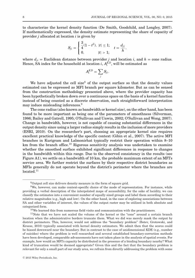
to characterize the kernel density function (De Smith, Goodchild, and Longley, 2007).If mathematically expressed, the density estimate representing the share of capacity ofprovider j allocated at location i is given by
Sji =⎧⎨⎩
34
(1 − t2), |t| ≤ 1;
0, |t| > 1;t = dji
h,
where dji = Euclidean distance between provider j and location i, and h = cone radius.Hence, SA index for the household at location i, AK D
i , will be estimated as
AK Di =
∑j
Sji.
We have adjusted the cell size8 of the output surface so that the density valuesestimated can be expressed as MFI branch per square kilometer. But as can be sensedfrom the construction methodology presented above, where the provider capacity hasbeen hypothetically broken down over a continuous space on the basis of a kernel functioninstead of being counted as a discrete observation, such straightforward interpretationmay induce misleading inferences.9
The cone radius (also known as bandwidth or kernel size), on the other hand, has beenfound to be more important as being one of the parameters of smoothness (Silverman,1986; Bailey and Gatrell, 1995; O’Sullivan and Unwin, 2002; O’Sullivan and Wong, 2007).Change in bandwidth, however, is not capable of causing substantial differences in theoutput density since using a larger radius simply results in the inclusion of more providers(ESRI, 2010). On the researcher’s part, choosing an appropriate kernel size requiresexcellent practical knowledge of the specific context (Gibin et al., 2007). The active MFIbranches in Kurigram and Lalmonirhat typically restrict their operation within 8–10km from the branch office.10 Rigorous sensitivity analysis was undertaken to examinewhether the smoothed surface exhibited significant differences in response to changesin the bandwidth within this range. Due to the observed consistency in the results (seeFigure A1), we settle on a bandwidth of 10 km, the probable maximum extent of an MFI’sservice area. We further restrict the surfaces by their respective district boundaries asMFIs generally do not operate beyond the district’s perimeter where the branches arelocated.11
8Output cell size delivers density measure in the form of square grid.9We, however, can make context-specific choice of the mode of representation. For instance, while
providing a verbal description of the interpolated maps of accessibility, for the sake of lucidity, we canclassify the estimates into a convenient number of equally sized groups and label them according to theirrelative magnitudes (e.g., high and low). On the other hand, in the case of exploring associations betweenSA and other variables of interest, the values of the output raster may be utilized in both absolute andcategorized form.
10We learned this from numerous field visits and communication with the practitioners.11Note that we have not scaled the volume of the kernel or the “cone” around a certain branch
location when the administrative borders truncate them. What we did was merely mask the output bydistrict perimeters. This, however, would not address the “boundary problem” (Botev, Grotowski, andKroese, 2010) typically associated with kernel density estimators. We admit then that the scores couldbe biased downward near the boundary. But in contrast to the case of unidimensional KDE (e.g., numberof suicides) where the problem is well researched and several established boundary-correction methodshave been developed, comparable advancements have not taken place in the analysis of spatial events. Forexample, how would an MFI’s capacity be distributed in the presence of a binding boundary nearby? Whatkind of truncation would be deemed appropriate? Given this and the fact that the boundary problem isrelevant for only a small part of our study area, we refrain from directly addressing the problem with some
C© 2015 Wiley Periodicals, Inc.

KHAN AND RABBANI: SPATIAL ACCESSIBILITY OF MICROFINANCE IN NORTHERN BANGLADESH 9
6. FINDINGS
SA of Microfinance in Kurigram and Lalmonirhat
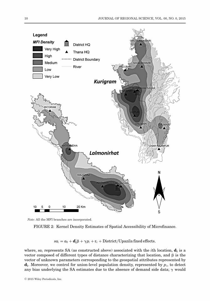
Figure 2 portrays a geointerpolated density surface12 produced by means of kernelsmoothing, which represents SA of microfinance in Kurigram and Lalmonirhat (followingthe methodology outlined above). Visual inspection reveals that there exists remark-able variability in accessibility across both Kurigram and Lalmonirhat. Furthermore,the geodistributional patterns exhibit significant similarity. In both cases, the degree ofconcentration in general tends to be markedly higher in the localities around the ad-ministrative headquarters (in particular, district and upazila headquarters). This is notsurprising because these areas are more urban in nature and, as a result, supposedly moreadvanced than others in terms of physical infrastructure (e.g., communication networksand utility services) and other amenities. The population residing over those regions isalso generally better off, considering both economic solvency and exposure to shocks (eco-nomic and natural), and will possibly be more preferred by the MFIs due to their highercredit demand.
Multivariate Analysis of SA and Microcredit Participation
Our rationalization of the detected variations in the SA of microfinance above, how-ever, is based on intuition and subjective perception rather than rigorous empirical in-vestigation. In order to verify the aforesaid graphical inferences, we now resort to thestandard practice of statistical inference to quantify the association of SA with other loca-tion attributes. Furthermore, we assess the explanatory power of the estimated SA indexfor household microborrowing.
In doing the latter, it is noteworthy that we are using a rather macroeconomic variable(SA) to explain the behavior at the micro (household) level (household microborrowing).Therefore, our SA index is a good candidate for satisfying the criterion of exogeneity.Should that be the case, the simple probit or Poisson models would be good enough toidentify the partial effect here, especially if region-specific fixed effects are accounted for.However, endogeneity might still be a source of concern due to other reasons. As Salim(2013) has demonstrated, MFIs strategically locate themselves, motivated by both profitmaximization and poverty outreach. Such nonrandom program placement, in particular,the focus on reaching out to the poor, would then suggest that the penetration of micro-finance operation would most possibly be correlated with both observed and unobservedhousehold attributes that are also crucial determinants of borrowing behavior. For exam-ple, in view of the revealed objective function of the MFIs, one might postulate a negativecorrelation between innate household ability and SA, hence introducing a downward biasin the estimated coefficients on the spatial access. As such, we will resort to an Instru-mental Variable (IV) framework to see if we can correct such bias and estimate a betterlower bound for the impact of spatial access on loan-taking behavior.
Geospatial Determinants of SA
Econometric specification. To discover and quantify the relationship between the geo-graphical accessibility and spatial background of a location, we estimate the followingOLS model:
(boundary) correction methods. We believe that this would not lead to a drastic revision of our findings,which have been shown to be robust to a number of other theoretical and empirical concerns.
12The software utilized is ESRI ArcGIS 9.3 C© with the Spatial Analyst C© extension.
C© 2015 Wiley Periodicals, Inc.
10 JOURNAL OF REGIONAL SCIENCE, VOL. 00, NO. 0, 2015
Note: All the MFI branches are incorporated.
FIGURE 2: Kernel Density Estimates of Spatial Accessibility of Microfinance.
sai = a0 + d′i� + �pi + εi + District/Upazila fixed effects,
where, sai represents SA (as constructed above) associated with the ith location, di is avector composed of different types of distance characterizing that location, and � is thevector of unknown parameters corresponding to the geospatial attributes represented bydi. Moreover, we control for union-level population density, represented by pi, to detectany bias underlying the SA estimates due to the absence of demand side data; � would
C© 2015 Wiley Periodicals, Inc.
KHAN AND RABBANI: SPATIAL ACCESSIBILITY OF MICROFINANCE IN NORTHERN BANGLADESH 11
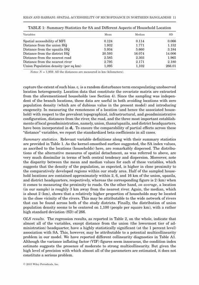
TABLE 1: Summary Statistics for SA and Different Aspects of Household Location
Variables Mean Median SD
Spatial accessibility of MFI 0.124 0.114 0.066Distance from the union HQ 1.932 1.771 1.152Distance from the upazila HQ 5.934 5.660 3.184Distance from the district HQ 20.593 16.074 14.006Distance from the nearest road 2.585 2.303 1.965Distance from the nearest river 2.795 2.171 2.180Union Population density (per sq km) 1,095 1,102 266.01
Notes: N = 1,959. All the distances are measured in km (kilometers).
capture the extent of such bias. εi is a random disturbance term encapsulating unobservedlocation heterogeneity. Location data that constitute the covariate matrix are extractedfrom the aforementioned households (see Section 4). Since the sampling was indepen-dent of the branch locations, these data are useful in both avoiding locations with zeropopulation density (which are of dubious value in the present model) and introducingexogeneity. In measuring the remoteness of a location (and hence the associated house-hold) with respect to the prevalent topographical, infrastructural, and geoadministrativeconfiguration, distances from the river, the road, and the three most important establish-ments of local geoadministration, namely, union, thana/upazila, and district headquarters,have been incorporated in di. To ensure the comparability of partial effects across these“distance” variables, we report the standardized beta coefficients in all cases.
Summary statistics. Relevant variable definitions along with their summary statisticsare provided in Table 1. As the kernel-smoothed surface suggested, the SA index values,as ascribed to the locations (households) here, are remarkably dispersed. The distribu-tions of the alternative measures of spatial detachment, as was referred to above, arevery much dissimilar in terms of both central tendency and dispersion. Moreover, notethe disparity between the mean and median values for each of these variables, whichsuggests that the density of the population, as expected, is higher in close proximity tothe comparatively developed regions within our study area. Half of the sampled house-hold locations are contained approximately within 2, 6, and 16 km of the union, upazila,and district headquarters, respectively, whereas the corresponding figure is 2 (km) whenit comes to measuring the proximity to roads. On the other hand, on average, a location(in our sample) is roughly 3 km away from the nearest river. Again, the median, whichis about 2 (km), shows that a relatively higher proportion of households may be locatedin the close vicinity of the rivers. This may be attributable to the wide network of riversthat can be found across both of the study districts. Finally, the distribution of unionpopulation density seems to be centered on 1,100 (people per square km), with a ratherhigh standard deviation (SD) of 266.
OLS results. The regression results, as reported in Table 2, on the whole, indicate thatalmost all of the variables, except distance from the union (the lowermost tier of ad-ministration) headquarter, have a highly statistically significant (at the 1 percent level)association with SA. This, however, may be attributable to a potential multicollinearityproblem in our model. We have reported different collinearity diagnostics in Table A1.Although the variance inflating factor (VIF) figures seem innocuous, the condition indexestimate suggests the presence of moderate to strong multicollinearity. But given thehigh level of precision with which almost all of the parameters are estimated, it does notconstitute a serious problem.
C© 2015 Wiley Periodicals, Inc.

12 JOURNAL OF REGIONAL SCIENCE, VOL. 00, NO. 0, 2015
TABLE 2: Geospatial Determinants of Spatial Accessibility (OLS)
Spatial Accessibility
Beta Coefficient
Variables (1) (2) (3)
Distance (in km) from theNearest river 0.455*** 0.456*** 0.463***
Nearest road −0.128*** −0.128*** −0.058***
District HQ −0.257*** −0.257*** −0.820***
Upazila HQ −0.307*** −0.306*** −0.339***
Union HQ −0.025* −0.025* −0.023*
Union population density 0.159*** 0.159*** 0.120***
Fixed effects No District UpazilaAdjusted R2 0.590 0.590 0.715
Notes: N = 1,959. Each observation represents a randomly chosen ultra-poor household. Fifteen householdlocations (only 0.76 percent of all) could not be used due to technical errors made in GIS data collection. Allregressions are OLS. Intercept and fixed-effect estimates are not reported to save space.
***P < 0.01, **P < 0.05, *P < 0.1.
In terms of directions (of the relationships), all the parameter estimates conform toour a priori expectations. Column (1) demonstrates this relationship, disregarding anygeoadministrative heterogeneity, whereas results reported in the latter two (i.e., columns(2) and (3)) control for district and upazila fixed effects. To elaborate, the farther a loca-tion (household) is from the nearest road and administrative headquarters, the lower thedegree of SA it is expected to experience. In contrast, distance from the nearest river is pos-itively associated with SA to microfinancial services. Focusing on the relative importanceof different types of distance in terms of partial effect, as reflected by the beta coefficients,results reveal that distances from the nearest river, upazila, and district headquartershave substantial association with SA. A one SD increase in the distance from the nearestriver is associated with an increase in SA of almost half SD, and the magnitude is fairlyrobust to the inclusion of fixed effects. On the other hand, irrespective of specification,the spatial separation from the upazila headquarter equivalent to one SD, ceteris paribus,reduces spatial access by at least 0.30 SD. A comparable relative movement in distancefrom the district headquarter is associated with no less than 0.25 SD lower SA (and aslarge as 0.82 SD once upazila-specific heterogeneity is partialled out). The correspondingfigure for detachment from the road ranges from 0.06 to 0.13 SD (in absolute value).The marginal impact of geographical detachment from the union headquarter, however,seems to be the least important in both practical and statistical terms. Union populationdensity, as one might conjecture, has a significant positive association with SA, but themagnitude, nonetheless, is small (namely, 0.16 SD at most). This, in turn, indicates thatour kernel estimates of SA could be biased upward (downward) in regions with higher(lower) population density but only slightly. As our results show, even after controllingfor population density, there seems to be other geospatial factors of higher substantivesignificance in the SA production function. Also note that a considerably large share ofvariation (59 and 71.5 percent) in SA has been explained by these location attributes.
We can therefore conclude that the remoteness of a location (household), definedin terms of geographical segregation from physical infrastructure and administrativeheadquarters, can have a remarkable bearing on its allocated degree of spatial accessto microfinancial services. Since better availability of infrastructure (which presumablyhas a high positive correlation with the existence of administrative establishments) and
C© 2015 Wiley Periodicals, Inc.

KHAN AND RABBANI: SPATIAL ACCESSIBILITY OF MICROFINANCE IN NORTHERN BANGLADESH 13
economic development are complementary to each other, the more isolated a household is,spatially speaking, from the comparatively “developed” regions, the lower the degree ofSA it will be provided with. Our results pertaining to the proximity to rivers also tend tosupport the MFIs’ objective of reaching out to poor households subject to financial sustain-ability and business viability. Being close to rivers in the northern areas of Bangladeshrepresents higher exposure to natural disasters such as floods and river erosions. Hence,we estimated the negative association between SA to financial services and proximity, asone would expect.
Microfinance Participation and SA
Econometric specification. To respond to the query as to whether the degree of spatialaccess to microfinance can explain both the incidence and extent of microborrowing (orin other words, realized access), we estimate two different models. In dealing with thepotential endogeneity problem in SA, as discussed briefly in Section 6, we make use ofinstruments in both cases.
To model the incidence of microborrowing, let y∗1i represent the unobserved propensity
of a household to borrow from an MFI (the so-called latent variable). Then the incidenceof microcredit participation, denoted by y1i, could be defined as
y1i ={
1 if y∗1i > 0,
0 if y∗1i ≤ 0.
The OLS model that we would estimate had there been data on y∗1i is given by
y∗1i = z′
i� + ui,
where zi = (y2i, x1i); y2i represents the standardized SA score for the ith household, x1iis a vector of exogenous household-level controls (see Table 3 for a complete list), and �denotes the vector of parameters corresponding to variables in zi. But as we discussedin Section 6, for consistent estimation, our setting requires the treatment of SA as anendogenous variable. We therefore model y2i as
y2i = x′i� + vi,
where xi= (x1i, x2i); x2i represents the set of instruments and � denotes the vector ofcoefficients associated with xi. Since the joint density function, f(y1i, y2i|xi), can be writ-ten as f(y1i|y2i, xi) f(y2i|xi), the log-likelihood function, in the presence of a continuousendogenous variable (namely, y2i), for observation i is given by
ln Li = y1i ln �(mi) + (1 − y1i) ln{1 − �(mi)} + ln Ø(
y2i − x′i�
�
)− ln �,(1)
where
mi = z′i� + � ( y2i−x′
i��
)(1 − �2)1/2 .
Here, �( − )and Ø( − ) are the standard normal cumulative and probability densityfunctions, respectively; � is the SD of vi; � is the correlation coefficient between ui andvi. That there might be an endogeneity problem is tantamount to the possibility that � �0. The model has been estimated by maximum likelihood estimation (MLE), and averagemarginal effects are computed to quantify and compare the partial impact of the variablesof interest.
C© 2015 Wiley Periodicals, Inc.
14 JOURNAL OF REGIONAL SCIENCE, VOL. 00, NO. 0, 2015
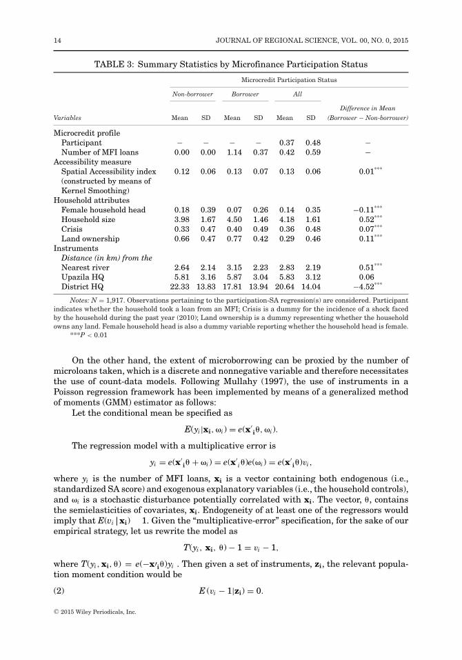
TABLE 3: Summary Statistics by Microfinance Participation Status
Microcredit Participation Status
Non-borrower Borrower All
Difference in MeanVariables Mean SD Mean SD Mean SD (Borrower − Non-borrower)
Microcredit profileParticipant − − − − 0.37 0.48 −Number of MFI loans 0.00 0.00 1.14 0.37 0.42 0.59 −
Accessibility measureSpatial Accessibility index(constructed by means ofKernel Smoothing)
0.12 0.06 0.13 0.07 0.13 0.06 0.01***
Household attributesFemale household head 0.18 0.39 0.07 0.26 0.14 0.35 −0.11***
Household size 3.98 1.67 4.50 1.46 4.18 1.61 0.52***
Crisis 0.33 0.47 0.40 0.49 0.36 0.48 0.07***
Land ownership 0.66 0.47 0.77 0.42 0.29 0.46 0.11***
InstrumentsDistance (in km) from theNearest river 2.64 2.14 3.15 2.23 2.83 2.19 0.51***
Upazila HQ 5.81 3.16 5.87 3.04 5.83 3.12 0.06District HQ 22.33 13.83 17.81 13.94 20.64 14.04 −4.52***
Notes: N = 1,917. Observations pertaining to the participation-SA regression(s) are considered. Participantindicates whether the household took a loan from an MFI; Crisis is a dummy for the incidence of a shock facedby the household during the past year (2010); Land ownership is a dummy representing whether the householdowns any land. Female household head is also a dummy variable reporting whether the household head is female.
***P < 0.01
On the other hand, the extent of microborrowing can be proxied by the number ofmicroloans taken, which is a discrete and nonnegative variable and therefore necessitatesthe use of count-data models. Following Mullahy (1997), the use of instruments in aPoisson regression framework has been implemented by means of a generalized methodof moments (GMM) estimator as follows:
Let the conditional mean be specified as
E(yi|xi, �i) = e(x′i, �i).
The regression model with a multiplicative error is
yi = e(x′i + �i) = e(x′
i)e(�i) = e(x′i)vi,
where yi is the number of MFI loans, xi is a vector containing both endogenous (i.e.,standardized SA score) and exogenous explanatory variables (i.e., the household controls),and �i is a stochastic disturbance potentially correlated with xi. The vector, , containsthe semielasticities of covariates, xi. Endogeneity of at least one of the regressors wouldimply that E(vi|xi) � 1. Given the “multiplicative-error” specification, for the sake of ourempirical strategy, let us rewrite the model as
T(yi, xi, ) − 1 = vi − 1,
where T(yi, xi, ) = e(−x′i)yi . Then given a set of instruments, zi, the relevant popula-tion moment condition would be
E (vi − 1|zi) = 0.(2)
C© 2015 Wiley Periodicals, Inc.
KHAN AND RABBANI: SPATIAL ACCESSIBILITY OF MICROFINANCE IN NORTHERN BANGLADESH 15
The consistent estimation of could then be carried out by GMM using the corre-sponding sample moments.
An explanation regarding the choice of controls and instruments is due. The en-dogeneity problem arises from the possibility that given the MFIs’ emphasis on povertyoutreach (subject to financial sustainability, of course), the locations which are more likelyto be chosen by these financial institutions would also be in a more disadvantageous posi-tion along both observed and unobserved dimensions. These attributes, more importantly,could have an independent and most probably negative impact on the likelihood of mi-crocredit participation. In statistical terms, this is equivalent to saying that we wouldexpect � < 0 and Corr (xi, �i) < 0 in models 1 and 2, respectively. This, in turn, couldlead to a downward bias in the estimated partial impact of SA on microborrowing. Underthese circumstances, consistent estimation with the help of instruments would requirefinding a variable that would be correlated with SA but would not have a partial impacton microloan take-up (after controlling for SA). In other words, a valid instrument wouldonly affect the dependent variable through its association with SA. In our context, weargue that “distance to the nearest river” can be such an instrument. Indeed, a house-hold living in close proximity to a river would be more prone to natural shocks and, as aresult, would be less likely to be a microborrower because of the higher risk associatedwith its portfolio. But this negative association is presumably working through the MFIs’decreased inclination to serve such a household due to its spatial disadvantage-inducedhigher potential credit risk, which is indeed supposed to be captured by the estimated SAscore. Hence, SA appears to be the component linking microloan take-up and proximity toriver along the causal chain. This and the fact that “distance to the nearest river” seemsto be the most robust predictor of SA (as the OLS results in Section 6 have shown) havepersuaded us to use it in our benchmark models. By the same token, however, the other“distance” variables, in particular, distance from the district and upazila HQ (which are,next to river-proximity, relatively strong predictors of SA),can serve the same purpose.Indeed, robustness analysis has been carried out using the whole set of potential instru-ments; the results remain more or less unaltered and hence have been reported in theAppendix (see Table A6).13
Apart from instruments, we have also included some variables representing the de-mographic and socioeconomic background of a household, which are potentially correlatedwith both its allocation of SA and microborrowing (but sufficiently predetermined so asnot to induce any reverse causality problem), namely, household size and dummies indi-cating any incidence of crisis, land possession, and whether the household head is female.On the other hand, since MFIs would presumably condition their presence on unobservedregional attributes, we also include district and upazila fixed effects in some of the modelsto be assured of the robustness of the benchmark parameter estimates.14
13As for the overidentification test results, please see Table A6. The results indicate that once theupazila fixed effects are accounted for, we cannot reject the null of all instruments being exogenous at asufficiently small level of significance. Hence, the evidence suggests that the instrument we have usedto generate the core results, viz., “distance to the nearest river,” satisfies the exclusionary restriction(after controlling for upazila heterogeneity). However, there is no definitive test for examining instrumentvalidity. Moreover, the tests that are typically used to this end could yield misleading results should therebe treatment effect heterogeneity (Angrist and Pischke, 2009).
14Our SA scores, however, are estimates and hence would entail measurement errors. But if the clas-sical errors-in-variables assumptions were in effect, this would most probably bias our estimators towardzero (Thoresen and Laake, 2000; Hausman, 2001; Edgerton and Jochumzen, 2003; Cameron and Trivedi,2005; Bateson and Wright, 2010). Hence, our estimators, in the worst-case scenario, would represent anunderestimation of the true population parameters in absolute value (allowing us to estimate a lower
C© 2015 Wiley Periodicals, Inc.
16 JOURNAL OF REGIONAL SCIENCE, VOL. 00, NO. 0, 2015
Summary statistics. Table 3 provides a summary description of the sampled households,differentiated by their microborrowing status, across a multitude of dimensions. Figuresshow that the microcredit take-up rate in our sample is 37 percent, and the (truncated)average number of loans is about 1. The borrowers seem to be better positioned in termsof spatial access to microfinancial services. Borrower households are typically larger andmore prone to crises (incidence of crisis is 7 percentage points higher). The share oflandless households is considerably lower (by around 11 percentage points) in the bor-rower subsample. Among the nonparticipants, about 18 percent of the households arefemale-headed, whereas the figure is only 7 percent among the participants. Moreover, asexpected, the microborrowers, on average, are closer to the district HQ as well as moredistant from the nearest river compared to the nonborrowers. The overall picture thatemerges therefore suggests that a typical microborrower household, despite being ob-served to be more likely to experience an exogenous shock, is wealthier and enjoys spatialproximity to district HQ, detachment from the river network, and (therefore) enhancedaccess to microfinancial services.
To further motivate the regression analysis, Figure 3 plots the participation rate andaverage number of loans, both unconditional and conditional (on participation), againstthe quartiles of SA. Both the loan take-up rate and (unconditional) average number ofloans exhibit a clear upward trend with increasing SA. The participation rate differentialbetween the two end quartiles is more than 11 percentage points—quite a substantialdifference. As expected, the truncated average number of loans schedule is flatter thanthe one without truncation but is still suggestive of a positive relationship with spatialaccess. This figure then lends some support to the hypothesis that the estimated SA indexcan explain the variations in microcredit participation. For the sake of a more preciseand statistically valid estimation of these relationships, we now resort to the regressionresults.
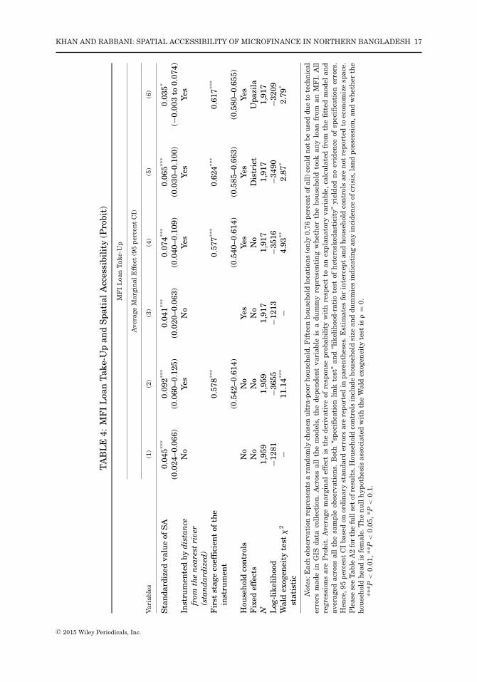
MFI loan take-up and SA: probit results. Table 4 reports the MLE estimates of averagemarginal effects from the probit model specified in Equation (1). For all the models,the key variable of interest is standardized SA. Additional household controls have beenincorporated in columns (3)–(6). Moreover, columns (5) and (6) include district and upazilafixed effects, respectively. Apart from columns (1) and (3), all other specifications entailthe use of “distance from the nearest river” as an instrument for SA.
For all specifications, we find a significant (average) marginal impact of SA on thelikelihood of microloan take-up (at the 1 percent level of significance, except the last case).Importantly, treating SA’s endogeneity by means of instrument leads to a substantial up-ward revision in the parameter estimate, thereby lending support to the hypothesizeddirection of bias earlier (see Section 6). The first-stage results, moreover, suggest that ourinstrument is indeed a strong predictor of spatial access in both practical and statisticalterms. The marginal effect estimate from the benchmark model including neither instru-ment nor other controls is more than doubled in response to the inclusion of instruments(a change from 0.045 to 0.092). Such upward revision is observed in the presence of house-hold controls too (0.074 compared to 0.041). Though the IV estimate becomes somewhatsmaller (and marginally significant) upon including district and upazila fixed effects, aone SD increase in SA, ceteris paribus, increases a household’s microcredit participationprobability by at least 3.5 percentage points. Using exogeneity tests, we found very weak
bound). Also, to make our case more cogent, inspired by the discussion in Angrist and Pischke (2009), wehave estimated OLS (and 2SLS) models (with heteroskedasticity-robust standard errors to take care of thepotential heteroskedasticity) for both incidence and extent of microborrowing. Interestingly, the estimatedmarginal effects are not sensitive to the choice of models. Please see Tables A4 and A5.
C© 2015 Wiley Periodicals, Inc.
KHAN AND RABBANI: SPATIAL ACCESSIBILITY OF MICROFINANCE IN NORTHERN BANGLADESH 17
TA
BL
E4:
MF
IL
oan
Tak
e-U
pan
dS
pati
alA
cces
sibi
lity
(Pro
bit)
MF
IL
oan
Tak
e-U
p
Ave
rage
Mar
gin
alE
ffec
t(9
5pe
rcen
tC
I)
Var
iabl
es(1
)(2
)(3
)(4
)(5
)(6
)
Sta
nda
rdiz
edva
lue
ofS
A0.
045**
*0.
092**
*0.
041**
*0.
074**
*0.
065**
*0.
035*
(0.0
24–0
.066
)(0
.060
–0.1
25)
(0.0
20–0
.063
)(0
.040
–0.1
09)
(0.0
30–0
.100
)(−
0.00
3to
0.07
4)In
stru
men
ted
byd
ista
nce
from
the
nea
rest
rive
r(s
tan
dar
diz
ed)
No
Yes
No
Yes
Yes
Yes
Fir
stst
age
coef
fici
ent
ofth
ein
stru
men
t0.
578**
*0.
577**
*0.
624**
*0.
617**
*
(0.5
42–0
.614
)(0
.540
–0.6
14)
(0.5
85–0
.663
)(0
.580
–0.6
55)
Hou
seh
old
con
trol
sN
oN
oYe
sYe
sYe
sYe
sF
ixed
effe
cts
No
No
No
No
Dis
tric
tU
pazi
laN
1,95
91,
959
1,91
71,
917
1,91
71,
917
Log
-lik
elih
ood
−128
1−3
655
−121
3−3
516
−349
0−3
209
Wal
dex
ogen
eity
test
2
stat
isti
c−
11.1
4***
−4.
93**
2.87
*2.
79*
Not
es:E
ach
obse
rvat
ion
repr
esen
tsa
ran
dom
lych
osen
ult
ra-p
oor
hou
seh
old.
Fif
teen
hou
seh
old
loca
tion
s(o
nly
0.76
perc
ent
ofal
l)co
uld
not
beu
sed
due
tote
chn
ical
erro
rsm
ade
inG
ISda
taco
llec
tion
.A
cros
sal
lth
em
odel
s,th
ede
pen
den
tva
riab
leis
adu
mm
yre
pres
enti
ng
wh
eth
erth
eh
ouse
hol
dto
okan
ylo
anfr
oman
MF
I.A
llre
gres
sion
sar
eP
robi
t.A
vera
gem
argi
nal
effe
ctis
the
deri
vati
veof
resp
onse
prob
abil
ity
wit
hre
spec
tto
anex
plan
ator
yva
riab
le,
calc
ula
ted
from
the
fitt
edm
odel
and
aver
aged
acro
ssal
lth
esa
mpl
eob
serv
atio
ns.
Bot
h“s
peci
fica
tion
lin
kte
st”
and
“lik
elih
ood-
rati
ote
stof
het
eros
keda
stic
ity”
yiel
ded
no
evid
ence
ofsp
ecif
icat
ion
erro
rs.
Hen
ce,9
5pe
rcen
tC
Iba
sed
onor
din
ary
stan
dard
erro
rsar
ere
port
edin
pare
nth
eses
.Est
imat
esfo
rin
terc
ept
and
hou
seh
old
con
trol
sar
en
otre
port
edto
econ
omiz
esp
ace.
Ple
ase
see
Tab
leA
2fo
rth
efu
llse
tof
resu
lts.
Hou
seh
old
con
trol
sin
clu
deh
ouse
hol
dsi
zean
ddu
mm
ies
indi
cati
ng
any
inci
den
ceof
cris
is,l
and
poss
essi
on,a
nd
wh
eth
erth
eh
ouse
hol
dh
ead
isfe
mal
e.T
he
nu
llh
ypot
hes
isas
soci
ated
wit
hth
eW
ald
exog
enei
tyte
stis
�=
0.**
*P<
0.01
,**P
<0.
05,*
P<
0.1.
C© 2015 Wiley Periodicals, Inc.

18 JOURNAL OF REGIONAL SCIENCE, VOL. 00, NO. 0, 2015
Note: The quartiles of SA are 0.085, 0.114, and 0.152.
FIGURE 3: Spatial Accessibility and Microfinance Participation.
evidence of overall endogeneity in our models, especially if we account for regional fixedeffects (columns (5)–(6), Tables 4 and 5). This supports sufficiency of using probit mod-els for valid identification after controlling for regional heterogeneity (as we claimed inSection 6).
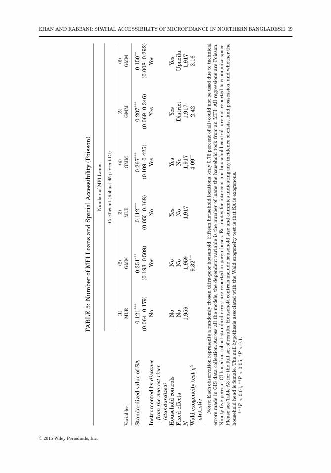
Number of MFI loans and SA: Poisson results. Table 5 gives the semielasticity estimatesfrom the Poisson model delineated in Equation (2). The different specifications used are inthe same order as above. The findings are also very consistent with those from the probitmodel. As before, the use of instruments appears to correct for the downward bias in theparameter estimate from models treating SA as exogenous. The increase in the expectednumber of MFI loans can be as high as 42 percent ([e(0.351) − 1]∗100) in response to aone SD rise in SA (and is always significant at the 5 percent level). Accounting for otherhousehold controls and district/upazila fixed effects, however, leads to a decline in theestimated impact, but it does not fall below 16 percent.15
To recapitulate, there is strong evidence that spatial access, as measured by theestimated SA index, can explain both the incidence and magnitude of microborrowing
15Furthermore, models where we used an “additive error” formulation yielded, in principle, the sameresults.
C© 2015 Wiley Periodicals, Inc.
KHAN AND RABBANI: SPATIAL ACCESSIBILITY OF MICROFINANCE IN NORTHERN BANGLADESH 19
TA
BL
E5:
Nu
mbe
rof
MF
IL
oan
san
dS
pati
alA
cces
sibi
lity
(Poi
sson
)
Nu
mbe
rof
MF
IL
oan
s
Coe
ffic
ien
t(R
obu
st95
perc
ent
CI)
(1)
(2)
(3)
(4)
(5)
(6)
Var
iabl
esM
LE
GM
MM
LE
GM
MG
MM
GM
M
Sta
nda
rdiz
edva
lue
ofS
A0.
121**
*0.
351**
*0.
112**
*0.
267**
*0.
207**
*0.
150**
(0.0
64–0
.179
)(0
.193
–0.5
09)
(0.0
55–0
.168
)(0
.109
–0.4
25)
(0.0
69–0
.346
)(0
.008
–0.2
92)
Inst
rum
ente
dby
dis
tan
cefr
omth
en
eare
stri
ver
(sta
nd
ard
ized
)
No
Yes
No
Yes
Yes
Yes
Hou
seh
old
con
trol
sN
oN
oYe
sYe
sYe
sYe
sF
ixed
effe
cts
No
No
No
No
Dis
tric
tU
pazi
laN
1,95
91,
959
1,91
71,
917
1,91
71,
917
Wal
dex
ogen
eity
test
2
stat
isti
c9.
32**
*4.
09**
2.42
2.16
Not
es:E
ach
obse
rvat
ion
repr
esen
tsa
ran
dom
lych
osen
ult
ra-p
oor
hou
seh
old.
Fif
teen
hou
seh
old
loca
tion
s(o
nly
0.76
perc
ent
ofal
l)co
uld
not
beu
sed
due
tote
chn
ical
erro
rsm
ade
inG
ISda
taco
llec
tion
.Acr
oss
all
the
mod
els,
the
depe
nde
nt
vari
able
isth
en
um
ber
oflo
ans
the
hou
seh
old
took
from
anM
FI.
All
regr
essi
ons
are
Poi
sson
.N
inet
y-fi
vepe
rcen
tC
Iba
sed
onro
bust
stan
dard
erro
rsar
ere
port
edin
pare
nth
eses
.Est
imat
esfo
rin
terc
ept
and
hou
seh
old
con
trol
sar
en
otre
port
edto
econ
omiz
esp
ace.
Ple
ase
see
Tab
leA
3fo
rth
efu
llse
tof
resu
lts.
Hou
seh
old
con
trol
sin
clu
deh
ouse
hol
dsi
zean
ddu
mm
ies
indi
cati
ng
any
inci
den
ceof
cris
is,l
and
poss
essi
on,a
nd
wh
eth
erth
eh
ouse
hol
dh
ead
isfe
mal
e.T
he
nu
llh
ypot
hes
isas
soci
ated
wit
hth
eW
ald
exog
enei
tyte
stis
that
SA
isex
ogen
ous.
***P
<0.
01,*
*P<
0.05
,*P
<0.
1.
C© 2015 Wiley Periodicals, Inc.

20 JOURNAL OF REGIONAL SCIENCE, VOL. 00, NO. 0, 2015
fairly well. Accounting for potential endogeneity in spatial access by means of instru-ment(s) further strengthens the case. By incorporating the geographical distribution of allrelevant MFI branches, our estimate of potential spatial access turns out to be an effectivepredictor of realized access.
7. DISCUSSION
In this study, we make a case to incorporate spatial distribution of microfinance pro-grams in the backdrop of overall concern around the issue of access to financial servicesfor the underprivileged and economically depressed households in Bangladesh. Micro-finance programs face the twin goals of reaching out to hard-to-reach poor householdswith borrowing constraints while remaining financially viable. The two objectives canbecome incompatible if MFIs are compelled to work in areas that are spatially remote(such as chars). So one can expect that spatial distribution of MFI activities will showa pattern that will correlate with the geospatial characteristics of a location. This papermakes a novel attempt to carry out a sophisticated analysis incorporating specific locationattributes using GIS and to the best of our knowledge, this study is the first of its kind toaddress this issue.
We have found that underlying geospatial characteristics such as distance from roads,rivers, and local administrative units can play a role in defining the spatial distribution ofmicrofinance access. While we focused on only two districts of Bangladesh (mainly becauseof availability of data), we believe the findings have external validity with respect to manyareas of Bangladesh due to topographical and infrastructural similarities. Geographicaccess is also an issue in many developing countries, especially in places such as Africa,South Asia, and Latin America. Hence, we believe our results may be broadly applicableto many other places and countries.
Our findings suggest that access to microfinance products (as measured with respectto the physical location of MFI branches) shows clear geographical variations. Therefore,depending on the location of the household, access to financial services will also varyat the household level. While the overall abilities and socioeconomic characteristics of ahousehold play important roles in it, just being at a location that is isolated for variousother reasons (such as rivers and roads) may hinder a household’s participation in thefinancial services offered by the microfinance industry. Indeed, our findings indicate thatspatial access to microfinance has a significant bearing on household borrowing frommicrofinance organizations. If we allow the fact that such borrowing is directly relatedto consumption smoothing and possibly growth, spatial distance and isolation can playfurther detrimental roles in a household’s poverty situation and destitute.
The cost of running a program at an isolated location can be high, and because of thedemand for smaller sized loans by households living in the more remote areas, the revenueearning is likely to be low. Therefore, households living in these areas are more likely tobe new borrowers, and it may be important for subsidies to play a role to further theoutreach of the industry. Hence, spatial access maps can help the policymakers identifygeographic pockets where the financial access is typically low. Moreover, our multivariateanalysis can suggest what factors are associated with the variation in SA.
Methodologically, simple regression results showing a relationship between thehousehold’s decision to borrow and the spatial access to finance may be spurious dueto endogeneity and biased because of omitting variables that may be correlated with SA.Microfinance providers target poor households that may have lower propensity or capacityto borrow from the MFIs (Salim, 2013). Hence, the simple regression estimates relatingspatial access and household borrowing decisions are likely to be biased downward. We
C© 2015 Wiley Periodicals, Inc.

KHAN AND RABBANI: SPATIAL ACCESSIBILITY OF MICROFINANCE IN NORTHERN BANGLADESH 21
make use of instrument(s) to correct the potential bias in the estimated coefficient for thespatial access variable. As expected, we find that simple estimates were indeed biaseddownward and we consistently get a higher coefficient from the IV models.
Our analysis of the SA of microfinance, however, can be questioned and criticizedon multiple grounds. First, we need to admit that the SA index constructed is rather“absolute” in the sense that more informative index would need to be normalized bypopulation. We did not have access to information on the geographical distribution ofpotential clients for our study area and therefore worked exclusively on the supply side.The supply side information was also inadequate due to lack of data on MFI capacity.Moreover, since KDE disperses a branch’s spatial influence over a continuous circularspace irrespective of the topographical pattern of that vicinity, it therefore increasesthe likelihood of service supply being lost to areas that are not “servable” in the sensethat they may not be inhabitable and/or marked by zero population density (Yang et al.,2006). Despite often being considered as a merit, KDE’s insensitiveness to geopolitical oradministrative boundaries can also contribute to such loss of provision capacity in thepresence of geographical constraints (e.g., rivers and lakes) which can remarkably limitresource mobilization. Finally, questions can be raised as to whether a Gaussian curvecan properly model the distribution of a branch’s supply capacity over its service area.
8. CONCLUDING REMARKS
The concept of SA, although widely appreciated and applied in other branches ofresearch (such as health care and crime), is relatively new in the context of microfinance.Capitalizing on their contributions and investigations, we approached the issue of accessto microfinance from a geographical perspective. We believe this exercise may pave theway for using GIS analysis in the context of competition and other issues. With the aid ofGIS data, as shown here, relevant spatial attributes can be easily extracted, represented,and utilized. We confined ourselves mainly to the construction and graphical representa-tion of SA (in Kurigram and Lalmonirhat), identification of its spatial determinants, andevaluation of its explanatory power for household borrowing behavior. Future researchendeavors along this line should aim to collect more data (from both demand and sup-ply side) to overcome the inadequacy of our estimation strategy. Moreover, since spatialsegregation of potential clients and MFI establishments may act as a significant barrierto the realization of efficient transactions, empirical studies can indeed be undertaken toverify the existence of market failure via moral hazard and/or adverse selection. It wouldalso be very intriguing if, by taking advantage of GIS, the major spatial factors that anMFI takes into consideration for making an optimal location choice could be identified.
C© 2015 Wiley Periodicals, Inc.

22 JOURNAL OF REGIONAL SCIENCE, VOL. 00, NO. 0, 2015
APPENDIX
Notes: The dark-shaded diamonds denote the parameter estimates associated with a bandwidth choice of 10km (from the SA-geoattributes regression, namely, Model 1, Table 2). The error bars, on the other hand, representthe confidence intervals for these estimates. Other diamonds represent estimates corresponding to bandwidthsof 8, 9, 11, and 12 km.
FIGURE A1: Regression Coefficients for Different Bandwidths.
TABLE A1: Collinearity Diagnostic Measures
Variables Variance Inflating Factor (VIF) Tolerance Factor R2
Distance (in km) from theNearest river 1.11 0.90 0.10Nearest road 1.40 0.72 0.28District HQ 1.23 0.81 0.19Upazila HQ 1.38 0.72 0.28Union HQ 1.07 0.93 0.07
Population density 1.55 0.65 0.35Mean VIF 1.29Condition index 20.70
C© 2015 Wiley Periodicals, Inc.

KHAN AND RABBANI: SPATIAL ACCESSIBILITY OF MICROFINANCE IN NORTHERN BANGLADESH 23
TA
BL
EA
2:M
FI
Loa
nT
ake-
Up
and
Spa
tial
Acc
essi
bili
ty(P
robi
t)—
Com
preh
ensi
veR
esu
lts
MF
IL
oan
Tak
e-U
p
Ave
rage
Mar
gin
alE
ffec
t(9
5pe
rcen
tC
I)
Var
iabl
es(1
)(2
)(3
)(4
)(5
)(6
)
Sta
nda
rdiz
edva
lue
ofS
A0.
045**
*0.
092**
*0.
041**
*0.
074**
*0.
065**
*0.
035*
(0.0
24–0
.066
)(0
.060
–0.1
25)
(0.0
20–0
.063
)(0
.040
–0.1
09)
(0.0
30–0
.100
)(–
0.00
3to
0.07
4)F
emal
eh
ouse
hol
d-h
ead
−0.1
65**
*−0
.165
***
−0.1
66**
*−0
.162
***
(−0.
235
to–0
.096
)(–
0.23
4to
–0.0
97)
(–0.
234
to–0
.097
)(–
0.22
8to
–0.0
95)
Hou
seh
old
size
0.03
3***
0.03
3***
0.03
2***
0.03
3***
(0.0
19–0
.047
)(0
.019
–0.0
47)
(0.0
18–0
.046
)(0
.019
–0.0
46)
Lan
dow
ner
ship
0.08
9***
0.08
3***
0.08
2***
0.05
4**
(–0.
137
to–0
.042
)(–
0.13
0to
–0.0
36)
(–0.
129
to–0
.034
)(–
0.10
1to
–0.0
06)
Inci
den
ceof
cris
is0.
047**
0.04
3*0.
038*
0.01
4(0
.003
–0.0
90)
(–0.
000
to0.
086)
(–0.
005
to0.
082)
(–0.
033
to0.
060)
Inst
rum
ente
dby
dis
tan
cefr
omth
en
eare
stri
ver
(sta
nd
ard
ized
)
No
Yes
No
Yes
Yes
Yes
Hou
seh
old
con
trol
sN
oN
oYe
sYe
sYe
sYe
sF
ixed
effe
cts
No
No
No
No
Dis
tric
tU
pazi
laN
1,95
91,
959
1,91
71,
917
1,91
71,
917
Log
-lik
elih
ood
−128
1−3
655
−121
3−3
516
−349
0−3
209
Wal
dex
ogen
eity
test
2
stat
isti
c−
11.1
4***
−4.
93**
2.87
*2.
79*
Not
es:E
ach
obse
rvat
ion
repr
esen
tsa
ran
dom
lych
osen
ult
ra-p
oor
hou
seh
old.
Fif
teen
hou
seh
old
loca
tion
s(o
nly
0.76
perc
ent
ofal
l)co
uld
not
beu
sed
due
tote
chn
ical
erro
rsm
ade
inG
ISda
taco
llec
tion
.A
cros
sal
lth
em
odel
s,th
ede
pen
den
tva
riab
leis
adu
mm
yre
pres
enti
ng
wh
eth
erth
eh
ouse
hol
dto
okan
ylo
anfr
oman
MF
I.A
llre
gres
sion
sar
eP
robi
t.A
vera
gem
argi
nal
effe
ctis
the
deri
vati
veof
resp
onse
prob
abil
ity
wit
hre
spec
tto
anex
plan
ator
yva
riab
le,
calc
ula
ted
from
the
fitt
edm
odel
and
aver
aged
acro
ssal
lth
esa
mpl
eob
serv
atio
ns.
Bot
h“s
peci
fica
tion
lin
kte
st”
and
“lik
elih
ood-
rati
ote
stof
het
eros
keda
stic
ity”
yiel
ded
no
evid
ence
ofsp
ecif
icat
ion
erro
rs.
Hen
ce,9
5pe
rcen
tC
Iba
sed
onor
din
ary
stan
dard
erro
rsar
ere
port
edin
pare
nth
eses
.Est
imat
esfo
rin
terc
ept
and
fixe
def
fect
sar
en
otre
port
edto
econ
omiz
esp
ace.
Th
en
ull
hyp
oth
esis
asso
ciat
edw
ith
the
Wal
dex
ogen
eity
test
is�
=0.
***P
<0.
01,*
*P
<0.
05,*
P<
0.1.
C© 2015 Wiley Periodicals, Inc.
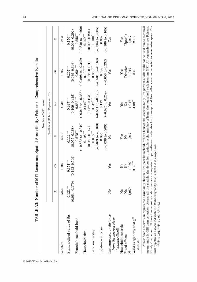
24 JOURNAL OF REGIONAL SCIENCE, VOL. 00, NO. 0, 2015
TA
BL
EA
3:N
um
ber
ofM
FI
Loa
ns
and
Spa
tial
Acc
essi
bili
ty(P
oiss
on)—
Com
preh
ensi
veR
esu
lts
Nu
mbe
rof
MF
IL
oan
s
Coe
ffic
ien
t(R
obu
st95
perc
ent
CI)
(1)
(2)
(3)
(4)
(5)
(6)
Var
iabl
esM
LE
GM
MM
LE
GM
MG
MM
GM
M
Sta
nda
rdiz
edva
lue
ofS
A0.
121**
*0.
351**
*0.
112**
*0.
267**
*0.
207**
*0.
150**
(0.0
64–0
.179
)(0
.193
–0.5
09)
(0.0
55–0
.168
)(0
.109
–0.4
25)
(0.0
69–0
.346
)(0
.008
–0.2
92)
Fem
ale
hou
seh
old-
hea
d−0
.572
***
−0.6
35**
*−0
.624
***
−0.5
58**
*
(−0.
835
to–0
.310
)(–
0.91
6to
–0.3
55)
(–0.
898
to–0
.349
)(–
0.84
8to
–0.2
69)
Hou
seh
old
size
0.10
8***
0.14
0***
0.13
9***
0.14
9***
(0.0
69–0
.147
)(0
.087
–0.1
93)
(0.0
86–0
.191
)(0
.093
–0.2
04)
Lan
dow
ner
ship
0.31
8***
0.34
2***
0.33
5***
0.18
0*
(–0.
469
to–0
.168
)(–
0.51
1to
–0.1
73)
(–0.
501
to–0
.169
)(–
0.36
4to
0.00
5)In
cide
nce
ofcr
isis
0.08
50.
117
0.08
80.
002
(–0.
039
to0.
209)
(–0.
025
to0.
259)
(–0.
056
to0.
232)
(–0.
160
to0.
165)
Inst
rum
ente
dby
dis
tan
cefr
omth
en
eare
stri
ver
(sta
nd
ard
ized
)
No
Yes
No
Yes
Yes
Yes
Hou
seh
old
con
trol
sN
oN
oYe
sYe
sYe
sYe
sF
ixed
effe
cts
No
No
No
No
Dis
tric
tU
pazi
laN
1,95
91,
959
1,91
71,
917
1,91
71,
917
Wal
dex
ogen
eity
test
2
stat
isti
c9.
32**
*4.
09**
2.42
2.16
Not
es:E
ach
obse
rvat
ion
repr
esen
tsa
ran
dom
lych
osen
ult
ra-p
oor
hou
seh
old.
Fif
teen
hou
seh
old
loca
tion
s(o
nly
0.76
perc
ent
ofal
l)co
uld
not
beu
sed
due
tote
chn
ical
erro
rsm
ade
inG
ISda
taco
llec
tion
.Acr
oss
all
the
mod
els,
the
depe
nde
nt
vari
able
isth
en
um
ber
oflo
ans
the
hou
seh
old
took
from
anM
FI.
All
regr
essi
ons
are
Poi
sson
.N
inet
y-fi
vepe
rcen
tC
Iba
sed
onro
bust
stan
dard
erro
rsar
ere
port
edin
pare
nth
eses
.Est
imat
esfo
rin
terc
ept
and
fixe
def
fect
sar
en
otre
port
edto
econ
omiz
esp
ace.
Th
en
ull
hyp
oth
esis
asso
ciat
edw
ith
the
Wal
dex
ogen
eity
test
isth
atS
Ais
exog
enou
s.**
*P<
0.01
,**P
<0.
05,*
P<
0.1.
C© 2015 Wiley Periodicals, Inc.

KHAN AND RABBANI: SPATIAL ACCESSIBILITY OF MICROFINANCE IN NORTHERN BANGLADESH 25
TA
BL
EA
4:M
FI
Loa
nT
ake-
Up
and
Spa
tial
Acc
essi
bili
ty(L
PM
)—C
ompr
ehen
sive
Res
ult
s
MF
IL
oan
Tak
e-U
p
Mar
gin
alE
ffec
t(9
5pe
rcen
tR
obu
stC
I)
Var
iabl
es(1
)(2
)(3
)(4
)(5
)(6
)
Sta
nda
rdiz
edva
lue
ofS
A0.
045**
*0.
097**
*0.
042**
*0.
078**
*0.
068**
*0.
035*
(0.0
24–0
.067
)(0
.059
–0.1
34)
(0.0
21–0
.064
)(0
.040
–0.1
16)
(0.0
31–0
.105
)(–
0.00
5to
0.07
5)F
emal
eh
ouse
hol
dh
ead
–0.1
42**
*–0
.146
***
–0.1
45**
*–0
.145
***
(–0.
200
to–0
.083
)(–
0.20
5to
–0.0
87)
(–0.
204
to–0
.086
)(–
0.20
4to
–0.0
85)
Hou
seh
old
size
0.03
2***
0.03
3***
0.03
2***
0.03
3***
(0.0
18–0
.046
)(0
.019
–0.0
47)
(0.0
18–0
.046
)(0
.018
–0.0
47)
Lan
dow
ner
ship
–0.0
86**
*–0
.081
***
–0.0
79**
*–0
.053
**
(–0.
132
to–0
.041
)(–
0.12
7to
–0.0
35)
(–0.
125
to–0
.033
)(–
0.10
0to
–0.0
06)
Inci
den
ceof
cris
is0.
046**
0.04
3*0.
038
0.01
1(0
.001
–0.0
91)
(–0.
002
to0.
088)
(–0.
007
to0.
084)
(–0.
037
to0.
060)
Inst
rum
ente
dby
dis
tan
cefr
omth
en
eare
stri
ver
(sta
nd
ard
ized
)
No
Yes
No
Yes
Yes
Yes
Fix
edef
fect
sN
oN
oN
oN
oD
istr
ict
Upa
zila
N1,
959
1,95
91,
917
1,91
71,
917
1,91
7A
dju
sted
R2
0.00
8–
0.05
00.
044
0.04
80.
100
Wal
dex
ogen
eity
test
2
stat
isti
c–
10.2
8***
–4.
90**
3.01
*2.
73*
Not
es:E
ach
obse
rvat
ion
repr
esen
tsa
ran
dom
lych
osen
ult
ra-p
oor
hou
seh
old.
Fif
teen
hou
seh
old
loca
tion
s(o
nly
0.76
perc
ent
ofal
l)co
uld
not
beu
sed
due
tote
chn
ical
erro
rsm
ade
inG
ISda
taco
llec
tion
.A
cros
sal
lth
em
odel
s,th
ede
pen
den
tva
riab
leis
adu
mm
yre
pres
enti
ng
wh
eth
erth
eh
ouse
hol
dto
okan
ylo
anfr
oman
MF
I.A
llre
gres
sion
sar
eL
PM
(Lin
ear
Pro
babi
lity
Mod
el).
Nin
ety-
five
perc
ent
CI
base
don
robu
stst
anda
rder
rors
are
repo
rted
inpa
ren
thes
es.E
stim
ates
for
inte
rcep
tan
dfi
xed
effe
cts
are
not
repo
rted
toec
onom
ize
spac
e.T
he
nu
llh
ypot
hes
isas
soci
ated
wit
hth
eW
ald
exog
enei
tyte
stis
that
SA
isex
ogen
ous.
***P
<0.
01,*
*P<
0.05
,*P
<0.
1.
C© 2015 Wiley Periodicals, Inc.
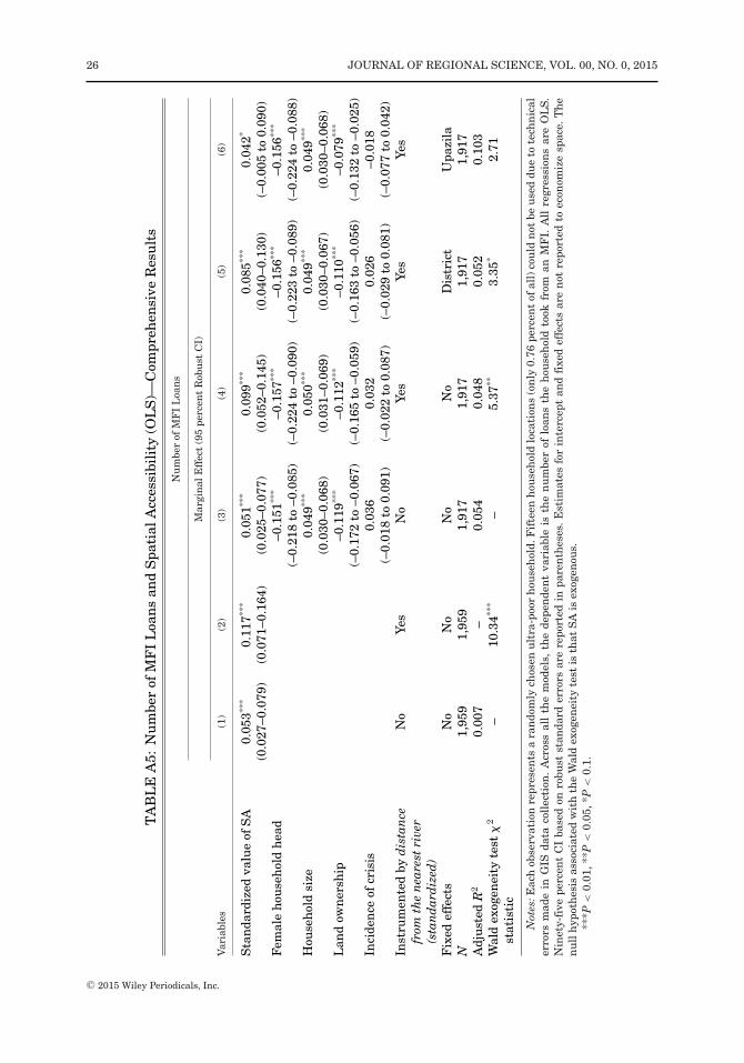
26 JOURNAL OF REGIONAL SCIENCE, VOL. 00, NO. 0, 2015
TA
BL
EA
5:N
um
ber
ofM
FI
Loa
ns
and
Spa
tial
Acc
essi
bili
ty(O
LS
)—C
ompr
ehen
sive
Res
ult
s
Nu
mbe
rof
MF
IL
oan
s
Mar
gin
alE
ffec
t(9
5pe
rcen
tR
obu
stC
I)
Var
iabl
es(1
)(2
)(3
)(4
)(5
)(6
)
Sta
nda
rdiz
edva
lue
ofS
A0.
053**
*0.
117**
*0.
051**
*0.
099**
*0.
085**
*0.
042*
(0.0
27–0
.079
)(0
.071
–0.1
64)
(0.0
25–0
.077
)(0
.052
–0.1
45)
(0.0
40–0
.130
)(–
0.00
5to
0.09
0)F
emal
eh
ouse
hol
dh
ead
–0.1
51**
*–0
.157
***
–0.1
56**
*–0
.156
***
(–0.
218
to–0
.085
)(–
0.22
4to
–0.0
90)
(–0.
223
to–0
.089
)(–
0.22
4to
–0.0
88)
Hou
seh
old
size
0.04
9***
0.05
0***
0.04
9***
0.04
9***
(0.0
30–0
.068
)(0
.031
–0.0
69)
(0.0
30–0
.067
)(0
.030
–0.0
68)
Lan
dow
ner
ship
–0.1
19**
*–0
.112
***
–0.1
10**
*–0
.079
***
(–0.
172
to–0
.067
)(–
0.16
5to
–0.0
59)
(–0.
163
to–0
.056
)(–
0.13
2to
–0.0
25)
Inci
den
ceof
cris
is0.
036
0.03
20.
026
–0.0
18(–
0.01
8to
0.09
1)(–
0.02
2to
0.08
7)(–
0.02
9to
0.08
1)(–
0.07
7to
0.04
2)In
stru
men
ted
byd
ista
nce
from
the
nea
rest
rive
r(s
tan
dar
diz
ed)
No
Yes
No
Yes
Yes
Yes
Fix
edef
fect
sN
oN
oN
oN
oD
istr
ict
Upa
zila
N1,
959
1,95
91,
917
1,91
71,
917
1,91
7A
dju
sted
R2
0.00
7–
0.05
40.
048
0.05
20.
103
Wal
dex
ogen
eity
test
2
stat
isti
c–
10.3
4***
–5.
37**
3.35
*2.
71
Not
es:E
ach
obse
rvat
ion
repr
esen
tsa
ran
dom
lych
osen
ult
ra-p
oor
hou
seh
old.
Fif
teen
hou
seh
old
loca
tion
s(o
nly
0.76
perc
ent
ofal
l)co
uld
not
beu
sed
due
tote
chn
ical
erro
rsm
ade
inG
ISda
taco
llec
tion
.A
cros
sal
lth
em
odel
s,th
ede
pen
den
tva
riab
leis
the
nu
mbe
rof
loan
sth
eh
ouse
hol
dto
okfr
oman
MF
I.A
llre
gres
sion
sar
eO
LS.
Nin
ety-
five
perc
ent
CI
base
don
robu
stst
anda
rder
rors
are
repo
rted
inpa
ren
thes
es.E
stim
ates
for
inte
rcep
tan
dfi
xed
effe
cts
are
not
repo
rted
toec
onom
ize
spac
e.T
he
nu
llh
ypot
hes
isas
soci
ated
wit
hth
eW
ald
exog
enei
tyte
stis
that
SA
isex
ogen
ous.
***P
<0.
01,*
*P<
0.05
,*P
<0.
1.
C© 2015 Wiley Periodicals, Inc.

KHAN AND RABBANI: SPATIAL ACCESSIBILITY OF MICROFINANCE IN NORTHERN BANGLADESH 27
TA
BL
EA
6:In
cide
nce
and
Ext
ent
ofM
icro
borr
owin
gan
dS
pati
alA
cces
sibi
lity
(Mu
ltip
leIn
stru
men
ts)
Pro
bit
Poi
sson
LP
MO
LS
MF
IL
oan
Tak
e-U
pN
um
ber
ofM
FI
Loa
ns
MF
IL
oan
Tak
e-U
pN
um
ber
ofM
FI
Loa
ns
Ave
rage
Mar
gin
alC
oeff
icie
nt
Coe
ffic
ien
tC
oeff
icie
nt
Eff
ect
(95
perc
ent
CI)
(Rob
ust
95pe
rcen
tC
I)(R
obu
st95
perc
ent
CI)
(Rob
ust
95pe
rcen
tC
I)
Var
iabl
es(1
)(2
)(3
)(4
)(5
)(6
)(7
)(8
)
Sta
nda
rdiz
edva
lue
0.09
1***
0.05
2***
0.33
2***
0.23
2***
0.09
4***
0.05
1***
0.11
3***
0.06
4***
ofS
A(0
.065
–0.1
18)
(0.0
23–0
.080
)(0
.211
–0.4
52)
(0.1
17–0
.348
)(0
.065
–0.1
23)
(0.0
22–0
.081
)(0
.077
–0.
150)
(0.0
28–
0.10
0)In
stru
men
ted
byd
ista
nce
sfr
omth
en
eare
stri
ver,
dis
tric
t,an
du
pazi
lah
ead
quar
ter
(all
stan
dar
diz
ed)
Yes
Yes
Yes
Yes
Yes
Yes
Yes
Yes
Fix
edef
fect
sD
istr
ict
Upa
zila
Dis
tric
tU
pazi
laD
istr
ict
Upa
zila
Dis
tric
tU
pazi
laO
veri
den
tifi
cati
onte
stst
atis
tic
24.0
8***
3.24
15.7
4***
6.12
**23
.31**
*2.
8316
.17**
*2.
59
Not
es:N
=1,
917.
All
mod
els
use
dist
ance
sfr
omth
en
eare
stri
ver,
dist
rict
,an
du
pazi
lah
eadq
uar
ter
(all
stan
dard
ized
)as
inst
rum
ents
.Eac
hob
serv
atio
nre
pres
ents
ara
ndo
mly
chos
enu
ltra
-poo
rh
ouse
hol
d.F
ifte
enh
ouse
hol
dlo
cati
ons
(on
ly0.
76pe
rcen
tof
all)
cou
ldn
otbe
use
ddu
eto
tech
nic
aler
rors
mad
ein
GIS
data
coll
ecti
on.
Hou
seh
old
con
trol
sar
ein
clu
ded
inal
lth
eca
ses.
Hou
seh
old
con
trol
sin
clu
deh
ouse
hol
dsi
zean
ddu
mm
ies
indi
cati
ng
any
inci
den
ceof
cris
is,l
and
poss
essi
on,a
nd
wh
eth
erth
eh
ouse
hol
dh
ead
isfe
mal
e.E
stim
ates
for
inte
rcep
t,h
ouse
hol
dco
ntr
ols,
and
fixe
def
fect
sar
en
otre
port
edto
econ
omiz
esp
ace.
As
for
over
iden
tifi
cati
onte
stst
atis
tics
,w
e’ve
use
dA
mem
iya–
Lee
–New
ey’s
stat
isti
cfo
rpr
obit
and
Han
sen
’sJ
-sta
tist
icfo
ral
loth
erm
odel
s.**
*P<
0.01
,**P
<0.
05,*
P<
0.1.
C© 2015 Wiley Periodicals, Inc.
28 JOURNAL OF REGIONAL SCIENCE, VOL. 00, NO. 0, 2015
REFERENCESAlessandrini, Pietro, Michele Fratianni, and Alberto Zazzaro. 2009. The Changing Geography of Banking and
Finance. London: Springer.Angrist, Joshua D. and Jorn-Steffen Pischke. 2009. Mostly Harmless Econometrics: An Empiricist’s Companion.
Princeton, NJ: Princeton University Press.Armendariz, Beatriz and Jonathan Morduch. 2005. The Economics of Microfinance. Cambridge, MA: The MIT
Press.Bailey, Trevor C. and Anthony C. Gatrell. 1995. Interactive Spatial Data Analysis. Essex: Longman.Bangladesh Bureau of Statistics (BBS). 2006. Final Report on Household Income Expenditure Survey-2005.
Dhaka, Bangladesh: BBS.——. 2011. Report on Household Income and Expenditure Survey-2010. Dhaka, Bangladesh: BBS.Bateson, Thomas F. and J. Michael Wright. 2010. “Regression Calibration for Classical Exposure Measurement
Error in Environmental Epidemiology Studies Using Multiple Local Surrogate Exposures,” American Journalof Epidemiology, 172(3), 344–352.
Beck, Thorsten, Asli Demirguc-Kunt, and Maria Soledad Martinez Peria. 2007. “Reaching Out: Access to and Useof Banking Services across Countries,” Journal of Financial Economics, 85(1), 234–266.
Binita, K.C. 2010. “Illinois Statewide Healthcare and Education Mapping,” Master’s Thesis, Graduate School,Southern Illinois University.
Botev, Zdravko I., Joseph F. Grotowski, and Dirk P. Kroese. 2010. “Kernel Density Estimation via Diffusion,”Annals of Statistics, 38(5), 2916–2957.
Cameron, A. Colin and Pravin K. Trivedi. 2005. Microeconometrics: Methods and Applications. Cambridge, UK:Cambridge University Press.
Cull, Robert, Asli Demirguc-Kunt, and Jonathan Morduch. 2009. “Microfinance Meets the Market,” Journal ofEconomic Perspectives, 23, 167–192.
De Smith, Michael J., Michael F. Goodchild, and Paul A. Longley. 2007. Geospatial Analysis. Leicester: TheWinchelsea Press.
Edgerton, David L. and Peter Jochumzen. 2003. “Estimation in Binary Choice Models with Measurement Errors,”Working Paper, Department of Economics, Lund University.
ESRI. 2010. “How Kernel Density Works,” Available online at: http://webhelp.esri.com/arcgisdesktop/9.3/index.cfm?TopicName=How%20Kernel%20Density%20works.
Fruttero, Anna and Varun Gauri. 2005. “The Strategic Choices of NGOs: Location Decisions in Rural Bangladesh,”The Journal of Development Studies, 41(5), 759–787.
Gibin, Maurizio, Paul Longley, and Phil Atkinson. 2007. “Kernel Density Estimation and Percent Volume Contoursin General Practice Catchment Area Analysis in Urban Areas,” Proceedings of the GIScience Research UKConference (GISRUK).
Goodman, David C., Elliott Fisher, Therese A. Stukel, and Chiang-hua Chang. 1997. “The Distance to CommunityMedical Care and the Likelihood of Hospitalization: Is Closer Always Better?” American Journal of PublicHealth, 87(7), 1144–1150.
Guagliardo, Mark F. 2004. “Spatial Accessibility of Primary Care: Concepts, Methods and Challenges,” Interna-tional Journal of Health Geographics, 3(1), doi:10.1186/1476-072X-3-3.
Hass, Kara. 2009. “Measuring Accessibility of Regional Parks: A Comparison of Three GIS Techniques,” Master’sThesis, San Jose State University.
Hausman, Jerry A. 2001. “Mismeasured Variables in Econometric Analysis: Problems from the Right and Prob-lems from the Left,” Journal of Economic Perspectives, 15(4), 57–68.
Hermes, Niels, Robert Lensink, and Aljar Meesters. 2011. “Outreach and Efficiency of Microfinance Institutions,”World Development, 39(6), 938–948.
Hossain, Mahabub. 1988. “Credit for Alleviation of Rural Poverty: The Grameen Bank in Bangladesh,” ResearchReport No. 65, International Food Policy Research Institute.
Hossain, Naomi, Mahfuza Haque, Rafiqul I. Sarkar, and Matiur Rahman. 2005. Inheriting Extreme Poverty:Household Aspirations, Community Attitudes and Childhood in Northern Bangladesh. Dhaka, Bangladesh:Save the Children, UK & BRAC-RED.
Khan, Abdullah A. and S. M. Bhardwaj. 1994. “Access to Health Care: A Conceptual Framework and Its Relevanceto Health Care Planning,” Evaluation & the Health Professions, 17, 60–76.
Longley, Paul A., Michael F. Goodchild, David J. Maguire, and David W. Rhind. 2005. Geographic InformationSystems and Science. West Sussex: John Wiley & Sons.
Luo, Wei and Fahui Wang. 2003. “Measures of Spatial Accessibility to Healthcare in a GIS Environment: Synthesisand a Case Study in Chicago Region,” Environment and Planning B, 30(6), 865–884.
Mahmud, Wahiduddin. 2011. “Mitigating Seasonal Hunger: Evidence from Northwest Bangladesh,” OccasionalPaper, Institute of Microfinance (InM).
McLafferty, Sara, and Sue Grady. 2004. “Prenatal Care Need and Access: A GIS Analysis,” Journal of MedicalSystems, 28(3), 321–333.
C© 2015 Wiley Periodicals, Inc.
KHAN AND RABBANI: SPATIAL ACCESSIBILITY OF MICROFINANCE IN NORTHERN BANGLADESH 29
McLafferty, Sara, Doug Williamson, and Philip G. McGuire. 1999. “Identifying Crime Hot Spots Using KernelSmoothing,” in V. Goldsmith, P. G. McGuire, J. B. Mollenkopf, and T. A. Ross (eds.), Analyzing Crime Patterns:Frontiers of Practice. Thousand Oaks, CA: Sage Publications, 77–85.
Mobarak, Mushfiq. 2011. Encouraging Seasonal Migration to Mitigate the Consequences of a Seasonal Famine inRural Bangladesh. Dhaka, Bangladesh: International Growth Centre.
Mullahy, John. 1997. “Instrumental-Variable Estimation of Count Data Models: Applications to Models ofCigarette Smoking Behavior,” The Review of Economics and Statistics, 79(4), 586–593.
Navajas, Sergio, Mark Schreiner, Richard L. Meyer, Claudio Gonzalez-Vega, and Jorge Rodriguez-Meza. 2002.“Microcredit and the Poorest of the Poor: Theory and Evidence from Bolivia,” World Development, 28, 333–346.
O’Sullivan, David and David Unwin. 2002. Geographic Information Analysis. New Jersey: John Wiley & Sons.O’Sullivan, David and David W. S. Wong. 2007. “A Surface-Based Approach to Measuring Spatial Segregation,”
Geographic Analysis, 39(2), 147–168.Oke, Joel T. O., R. Adeyemo, and Mure U. Agbonlahor. 2007. “An Empirical Analysis of Microcredit Repayment
in Southwestern Nigeria,” Humanities and Social Sciences Journal, 16(4), 63–74.Pedrosa, Jose and Quy Toan Do. 2011. “Geographic Distance and Credit Market Access in Niger,” African Devel-
opment Review, 23, 289–299.Presbitero, Andrea F. and Roberta Rabellotti. 2014. “Geographical Distance and Moral Hazard in Microcredit:
Evidence from Colombia,” Journal of International Development, 26(1), 91–108.Rahman, Rushidan I. 1996.“Impact of Grameen Krishi Foundation on the Socioeconomic Condition of Rural
Households,” Working Paper No. 7, Bangladesh Institute of Development Studies.Roslan, Abdul H. and Mohd Z. A. Karim. 2009. “Determinants of Microcredit Repayment in Malaysia: The Case
of Agrobank,” Humanities and Social Sciences Journal, 4(1), 45–52.Salim, Mir M. 2013.“Revealed Objective Functions of Microfinance Institutions: Evidence from Bangladesh,”
Journal of Development Economics, 104, 34–55.Schuurman, Nadine, Myriam Berube, and Valorie A. Crooks. 2010. “Measuring Potential Spatial Access to Pri-
mary Health Care Physicians Using a Modified Gravity Model,” The Canadian Geographer, 54(1), 29–45.Silverman, Bernard W. 1986. Density Estimation for Statistics and Data Analysis. New York: Chapman and Hall.Spencer, John and Gustavo Angeles. 2007. “Kernel Density Estimation as a Technique for Assessing Availability
of Health Services in Nicaragua,” Health Service Outcomes Research Method, 7(3–4), 145–157.Thoresen, Magne and Petter Laake. 2000. “A Simulation Study of Measurement Error Correction Methods on
Logistic Regression,” Biometrics, 56(3), 868–872.World Bank. 2008. Finance for All? Policies and Pitfalls in Expanding Access. Washington, DC: The World Bank.Xie, Zhixiao and Jun Yan. 2008. “Kernel Density Estimation of Traffic Accidents in a Network Space,” Computers,
Environment and Urban Systems, 32(5), 396–406.Yang, Duck-Hye, Robert Goerge, and Ross Mullner. 2006. “Comparing GIS-Based Methods of Measuring Spatial
Accessibility to Health Services,” Journal of Medical Systems, 30(1), 23–32.Zeller, Manfred, Manohar Sharma, Carla Henry, and Cecile Lapenu. 2001. An Operational Tool for Evaluating
Poverty Outreach of Development Policies and Projects. Washington, DC: International Food Policy ResearchInstitute, 45.
Zohir, Sazzad, Abantee Harun, Naser Farid, and Iftekharul Huq. 2007. “Implementation of Policies for ReducingChronic Poverty PRS Country Study:Bangladesh,” Background Paper for the Chronic Poverty Report 2008–09,ERG, CPRC and ODI.
Zug, Sebastian. 2006. “Monga—Seasonal Food Insecurity in Bangladesh —Bringing the Information Together,”The Journal of Social Studies, 111, 1–14.
C© 2015 Wiley Periodicals, Inc.