assessing the reliability of textbook data in syntax: adger’s core syntax · ·...
TRANSCRIPT

Assessing the reliability of textbook datain syntax: Adger’s Core Syntax1
JON SPROUSE
Department of Cognitive Sciences, University of California, Irvine
DIOGO ALMEIDA
Department of Linguistics and Languages, Michigan State University
(Received 1 February 2011; revised 12 October 2011)
There has been a consistent pattern of criticism of the reliability of acceptability
judgment data in syntax for at least 50 years (e.g., Hill 1961), culminating in several
high-profile criticisms within the past ten years (Edelman & Christiansen 2003,
Ferreira 2005, Wasow & Arnold 2005, Gibson & Fedorenko 2010, in press). The
fundamental claim of these critics is that traditional acceptability judgment collection
methods, which tend to be relatively informal compared to methods from exper-
imental psychology, lead to an intolerably high number of false positive results. In this
paper we empirically assess this claim by formally testing all 469 (unique, US-English)
data points from a popular syntax textbook (Adger 2003) using 440 naıve partici-
pants, two judgment tasks (magnitude estimation and yes–no), and three different
types of statistical analyses (standard frequentist tests, linear mixed effects models,
and Bayes factor analyses). The results suggest that the maximum discrepancy be-
tween traditional methods and formal experimental methods is 2%. This suggests that
even under the (likely unwarranted) assumption that the discrepant results are all
false positives that have found their way into the syntactic literature due to the
shortcomings of traditional methods, the minimum replication rate of these 469 data
points is 98%. We discuss the implications of these results for questions about the
reliability of syntactic data, as well as the practical consequences of these results for
the methodological options available to syntacticians.
1. IN T R O D U C T I O N
There are two undisputable facts concerning data collection in the field of
generative syntax: (i) Acceptability judgments form a substantial component
of the empirical foundation of generative syntax (Chomsky 1965, Schutze
[1] This research was supported in part by National Science Foundation grant BCS-0843896 toJon Sprouse. We would like to thank Carson Schutze, Colin Phillips, James Myers andthree anonymous JL referees for helpful comments on earlier drafts. We would also like tothank Andrew Angeles, Melody Chen, and Kevin Proff for their assistance constructingmaterials. All errors remain our own.
J. Linguistics 48 (2012), 609–652. f Cambridge University Press 2012doi:10.1017/S0022226712000011 First published online 8 February 2012
609
1996), and (ii) the vast majority of the acceptability judgments that have been
reported in the generative syntax literature over the past 50 years were col-
lected informally, that is, without either the use of formal data collection
protocols, nor scrutiny via the statistical analysis techniques that are familiar
from experimental psychology. The informality with which acceptability
judgments are traditionally collected has led to a steady stream of metho-
dological criticisms since the earliest days of generative syntax (e.g., Hill 1961,
Spencer 1973), culminating in a particularly dramatic increase in methodo-
logical discussions over the past 15 years, presumably due to the relative ease
with which formal acceptability judgment can be constructed, deployed, and
analyzed using freely available software and internet-based participant pools
(Bard, Robertson & Sorace 1996; Keller 2000, 2003; Edelman & Christiansen
2003; Phillips & Lasnik 2003; Featherston 2005a, b, 2007, 2008, 2009;
Ferreira 2005; Sorace & Keller 2005; Wasow & Arnold 2005; Alexopoulou
& Keller 2007; den Dikken, Bernstein, Tortora & Zanuttini 2007;
Fanselow 2007; Newmeyer 2007; Sprouse 2007a, b, 2008, 2009, 2011a, b;
Culbertson & Gross 2009; Myers 2009; Phillips 2009; Bader & Haussler
2010; Culicover & Jackendoff 2010; Dabrowska 2010; Fedorenko & Gibson
2010; Gibson & Fedorenko 2010, in press ; Gross & Culbertson 2011; Weskott
& Fanselow 2011; Sprouse & Almeida 2011, 2012; Sprouse, Fukuda, Ono &
Kluender 2011 ; Sprouse, Schutze & Almeida 2011; Sprouse, Wagers &
Phillips 2012).
One oft-repeated claim in this literature is that traditional methods are
somehow unreliable, resulting in the construction of ill-supported syntactic
theories (e.g., Edelman & Christiansen 2003, Ferreira 2005, Wasow &
Arnold 2005, Gibson & Fedorenko 2010, in press). Our goal in this paper is
to address this claim empirically by testing all of the unique, US-English
language data points found in a recent (and popular) generative syntax
textbook (Core Syntax by David Adger, 2003, Oxford University Press). Our
hope is that by testing a large set of data points (469 sentence types forming
365 statistical comparisons) that cover a wide range of syntactic phenomena
(nine distinct topic-oriented chapters) and form a comprehensive introduc-
tion to (generative) syntax we will be able to provide a relatively accurate
estimate of the reliability of the data that is central to generative syntactic
theory. Of course, the generalizability of this estimate depends entirely on
how representative of the field one finds the textbook – a subjective issue that
is likely to vary from researcher to researcher (see Section 8 for discussion).
However, we believe that testing such a large set of data will provide a much
better estimate of the reliability of syntactic data than the relatively small
proof-of-concept studies that have been conducted to date (e.g., Wasow &
Arnold 2005, Gibson & Fedorenko in press). These proof-of-concept studies
typically suffer from both limited amounts of data (typically fewer than
10 sentence types) and biased selection of phenomena (they typically only
report replication failures, not successful replications). We believe that the
J O N S P R O U S E & D I O G O A L M E I D A
610

only way to truly address the question of whether there is an epidemic of
unreliable data in syntactic theory is to compare the ratio of replication
failures to successful replications for a large sample of phenomena.
2. DE F I N I N G R E L I A B I L I T Y
Although the word unreliable has an intuitive meaning to most readers,
formally there are (at least) two types of unreliability that are relevant to the
evaluation of an experiment. The first type of unreliability concerns FALSE
POSITIVES, which occur when an experiment reports a difference between two
(or more) conditions, but no difference truly exists (false positives are also
known as Type I errors). The second type of unreliability concerns FALSE
NEGATIVES, which occur when an experiment reports no difference between
two (or more) conditions, but there is, in fact, a difference between the con-
ditions (false negatives are also known as Type II errors). It is important to
note that these two types of unreliability, though related, are not treated
equally in the experimental psychology literature. False positives are gener-
ally considered more detrimental to scientific research than false negatives,
primarily because of the assumption that scientific theories are constructed
from differences between conditions (i.e., positive results), not invariances
between conditions (i.e., negative results).2 This asymmetry can be clearly
seen in the statistical best practices of the field: whereas the criterion for
inferring a positive result under null hypothesis testing is p<.05, which
would result in a maximum 5% false positive rate if applied consistently
(Nickerson 2000), the suggested maximum false negative rate is FOUR TIMES
HIGHER – 20% (Cohen 1962, 1988, 1992). This suggests that, as a rule of
thumb, experimental psychologists view false positives as four times more
detrimental than false negatives (Cohen 1992). Though the definition of tol-
erable and intolerable false positive and false negative rates is ultimately
subjective, in general we can say that an experimental protocol is reliable if it
produces both a very low rate of false positives AND a tolerable rate of false
negatives.
With these definitions in place, we can see that there are in fact two types
of criticisms that can be levied at traditional experimental methods in syntax:
1. Traditional methods are unreliable because they have an intolerably high
FALSE POSITIVE rate. The corollary of this is that formal experiments are
more reliable because they have a lower false positive rate.
[2] False negatives are more commonly discussed as STATISTICAL POWER, which is simply anintuitive recasting of false negatives in terms of true positives: statistical power is the abilityof an experiment to detect a difference when one truly exists. To calculate statistical power,simply subtract the false negative rate (b) from 100%. The resulting percentage, such as thetarget rate of 80% (suggested by Cohen 1992), means that a true difference will be detected80% of the time, and the other 20% of the time the experiment will report a false negative.
R E L I A B I L I T Y O F T E X T B O O K D A T A I N S Y N T A X
611

2. Traditional methods are unreliable because they have an intolerably
high FALSE NEGATIVE rate. The corollary of this is that formal
experiments are more reliable because they have a lower false negative
rate.
Criticisms of traditional methods have primarily focused on false
positives (Wasow & Arnold 2005, Gibson & Fedorenko in press), perhaps
because of the aforementioned assumption in experimental psychology
that false positives are more detrimental than false negatives. Because
false positives have been the primary focus of many critics, we will focus
almost exclusively on false positives in this article. However, it is important
to note that it is possible that the consequences of false negatives on syntactic
theory are greater than the consequences of false negatives on other
psychological theories. Syntacticians often attempt to capture both differ-
ences between sentences and invariances between sentences in grammatical
theories, such that false negatives may have an impact on theory construc-
tion that it is similar to that of false positives. Several researchers have
investigated whether traditional methods lead to more false negatives
than formal methods, at least for individual phenomena, by re-testing
classic phenomena with formal experiments and looking for subtle patterns
in the data that may have been overlooked by traditional methods (e.g., Bard
et al. 1996, Keller 2000, Featherston 2005b, Alexopoulou & Keller 2007,
Sprouse, Fukuda, Ono & Kluender 2011). Taking a slightly different
tack, Sprouse & Almeida (2011) compared the false negatives/statistical
power of two types of acceptability judgment experiments, magnitude esti-
mation and forced-choice, for 95 phenomena that span the range of possible
effect sizes in syntax and found evidence that suggests that traditional ac-
ceptability judgment experiments may in fact be MORE POWERFUL at detecting
differences between sentence types than formal experiments, contrary to
common assumptions. Clearly both false positives and false negatives have a
role to play in assessing the reliability of data in syntax; nonetheless, for the
current article, we will focus primarily on false positives, and refer interested
readers to the above-mentioned references for a fuller discussion of false
negatives.
In the sections that follow, we will compare the traditionally collected
judgments reported in Adger (2003) to the results of two formal acceptability
judgment experiments in an attempt to estimate the false positive rate in
this data set. At this point, the problem with this comparison should be clear :
to determine the false positive rate, we need a list of the true positives, but all
we have are the results of two types of experiments (traditional, informal
experiments and formal experiments), each of which are susceptible to
both false positives and false negatives. To get around this, we will evaluate
these results in a two-step process. First, we will simply assume that
the results of the formal experiments reveal all and only true positives.
J O N S P R O U S E & D I O G O A L M E I D A
612

This is very much in line with the assumptions of many critics of traditional
methods, therefore it will allow us to evaluate their concerns on their own
terms. Because the negative results of the formal experiments are either true
negatives or false negatives, the replication rate derived from comparing the
Adger (2003) results to the formal results is the minimum replication rate
for this particular data set (i.e., the replication rate could be higher than this
number, but it cannot be lower). Then we will take a closer look at the
phenomena that did not replicate in the formal experiment (i.e., the negative
results) to better determine whether they are likely true negatives, which
means that they were false positives in Adger (2003), or whether they are
likely false negatives, which means that they were true positives in Adger
(2003). Although we can offer no definitive conclusions about the status of
the negative results from the formal experiments, we believe the discussion
will help readers to refine the replication estimate for this particular data set
for themselves.
3. TH E D A T A P O I N T S I N AD G E R (2003)
The procedure for identifying the data points in Adger (2003) was as follows:
First, all examples that were obviously not data points (syntactic trees,
terminological definitions, etc.) were excluded. This yielded 873 data-like
examples, which were sorted into the following categories :
Pattern: These are sentences that are reported as part of a group of
two or more sentence types that form a pattern of accept-
ability as is standard in generative syntax. A pattern always
included at least one starred example and one un-starred
example.
Existence: These are sentences that were used to demonstrate the exist-
ence or inexistence of a given construction in English.
Repeats: As a textbook, some sentences are repeated for expository or
pedagogical reasons.
Not English: These are examples that are non-English. We included non-US
and non-standard dialects of English (as defined by Adger)
in this category because the participant population in our
experiments was native US-English speakers.
Untestable : These are sentences that required a task different from ac-
ceptability judgment. For example, some data in syntax is
based on the availability or unavailability of specific inter-
pretations or readings of a potentially ambiguous string of
words. These cannot be tested using a standard judgment
survey.
The distribution of data-like examples in Adger (2003) is given in Table 1.
Though we attempted to apply the above criteria consistently throughout the
R E L I A B I L I T Y O F T E X T B O O K D A T A I N S Y N T A X
613

entire textbook, it is possible that some readers may disagree with a few of
the classifications. Nonetheless, we believe that the classification in Table 1 is
by-and-large correct.
The 261 tokens that were categorized as pattern examples represented
198 distinct sentence types (i.e., there were 63 structural repeats). Twenty-
one of those sentence types were presented without an explicit control
condition, though the intended control condition was described in the text
(e.g., by discussing the grammatical operation that led to the unaccept-
ability). Therefore we constructed 21 additional sentence types to serve as
the grammatical control conditions for these sentence types. The resulting
219 sentence types (198+21) served as the conditions of the magnitude
experiments (ME) described in Section 5 below. We chose magnitude
estimation to test the pattern sentence types because the empirical claim
in Adger (2003) is that there is a relative difference (or pattern) in ac-
ceptability among these sentence types, and magnitude estimation has
been proposed as a good method for assessing relative differences in ac-
ceptability (Bard et al. 1996, Cowart 1997, Keller 2000, Featherston 2005a;
for more cautious endorsements, see Bader & Haussler 2010, Sprouse 2011b,
Weskott & Fanselow 2011). The 250 existence tokens became the target
materials for the yes–no experiments, which are described in Section 6 be-
low. We chose the yes–no task to test the existence tokens because the
empirical claim in Adger (2003) is that these constructions are possible in
US English (a fact that could also be investigated by using a representative
corpus of US English). All but three of the existence tokens were un-starred
in the text, and presented without any discussion of potential comparison
conditions. Three starred examples were also included in the existence ca-
tegory because there was no discussion of an explicit acceptable compari-
son condition or a grammatical operation that could be used to construct
an appropriate comparison condition. The 219 conditions from the ME
experiments were combined with the 250 existence tokens from the yes–no
experiments to form the 469 data points referenced in the introduction.
Tokens Percentage
Pattern 261 29.9%
Existence 250 28.6%
Repeats 124 14.2%
Not English 144 16.5%
Untestable 94 10.8%
Total 873
Table 1The distribution of data-like examples in Adger (2003).
J O N S P R O U S E & D I O G O A L M E I D A
614

The repeat, non-English, and untestable tokens were not tested in the ex-
periments.
4. TH E C R I T E R I A F O R D I S C R I M I N A T I N G S U C C E S S F U L R E P L I C A T I O N S
A N D R E P L I C A T I O N F A I L U R E S
Data analysis and interpretation are often glossed over in articles that
are critical of traditional methods, leaving the perception that one simply
plugs the data into a statistical test, and then the test tells you whether
the experimental hypothesis is true or false. Unfortunately, the situation
is often much more complex than this. Not only are there many different
statistical tests available for any given experimental design, but there are
also several different inferential methods that can be used to draw conclu-
sions about the experimental hypothesis from any given set of statistics.
A full discussion of statistical tests and types of inference is clearly
beyond the scope of this article ; however, we can be explicit about the stat-
istical and inferential assumptions that will underlie the data analysis in this
article.
For the magnitude estimation experiments, we will define replication as
the simple detection of a significant difference in the correct direction be-
tween the conditions in a phenomenon. For example, if a phenomenon
consisted of two conditions, a replication obtains if the sentence reported
as more acceptable by Adger (usually through the lack of a diacritic) is
observed to be significantly more acceptable than the sentence reported as
less acceptable by Adger (through the presence of a diacritic). Similarly, for
the yes–no experiments, we will define replication as the observation of sig-
nificantly more yes-responses than no-responses for the sentences that were
reported as grammatical by Adger, and as the reverse (more no-responses
than yes-responses) for the sentences that were reported as ungrammatical
by Adger. In other words, for grammatical sentences the proportion of
yes-responses must be significantly greater than .5, and for ungrammatical
sentences the proportion of no-responses must be significantly greater than .5.
It is clearly possible to imagine other definitions of replication. For ex-
ample, for the ME experiments one could require that the numerical ratings
meet certain thresholds in addition to reaching statistical significance in the
correct direction. As a concrete example, one could specify that un-starred
sentences in Adger must be rated above 0.5 on a z-unit scale (the standar-
dized scale that is the result of a z-score transformation; see Schutze &
Sprouse in press for a review), and starred sentences must be rated lower than
x0.5 on a z-unit scale in order for Adger’s claim to be replicated. Similarly,
one could also specify that only significant differences of a certain magnitude
(e.g., greater than 0.75 z-units) should count as significant differences. For
the yes–no experiments, one could specify that the proportion of desired
responses must be significantly larger than a threshold other than 0.5, such as
R E L I A B I L I T Y O F T E X T B O O K D A T A I N S Y N T A X
615

0.75, which would mean that more than three quarters of participants must
find rate the sentence the same as Adger (2003).
We chose not to impose these extra restrictions on the definition of repli-
cation for several reasons. First and foremost, we believe that the simple
detection of a difference in the predicted direction is closest to the intent of
Adger (2003). Adger (2003) primarily uses un-starred and starred sentences,
as opposed to the full range of diacritics available to syntacticians, suggest-
ing that he is primarily concerned with the existence of the difference, and
not the magnitude of the difference, or the absolute location of the ratings on
the acceptability continuum. Second, the imposition of additional numerical
criteria on the analysis requires an explicit hypothesis about the effect of
syntactic (i.e., grammatical) manipulations on acceptability judgments.
Acceptability judgments are a behavioral response that is directly affected by
several different aspects of the language faculty, of which syntax is only one
(others include lexical semantics, compositional semantics, and even parsing
difficulty). While it may be possible someday to create a complex theory of
acceptability judgments that makes fine-grained predictions about specific
levels of acceptability, we do not have one yet (see also Section 8 below). In
the absence of such a theory, and in the absence of explicit hypotheses for-
mulated by the author, we feel as though extra numerical constraints are
impossible to specify objectively, as different researchers are likely to have
different assumptions about what is a reasonable hypothesis. Given all of
these reasons, we felt the most appropriate definition would be a simple
significant difference in the correct direction; however, in Appendix A we do
report the numerical ratings from the ME experiment, and in Appendix B we
report the number of yes-responses from the yes–no experiments, so that
readers may evaluate the differences for themselves.
Up to this point we have intentionally left the definition of STATISTICALLY
SIGNIFICANT vague. This is because we decided to analyze the results using
three different types of statistical tests. First, we calculated classic p-values
using standard frequentist tests (t-tests for 2-sentence phenomena, one-way
ANOVAs for 3-sentence phenomena, two-way ANOVAs for 4-sentence
phenomena, and sign-tests for yes–no results). Second, because there has
been growing interest in the use of linear mixed-effects models (LMEMs) for
the analysis of language data, we ran linear mixed-effect models with two
random factors : participants and items. We used the PVALS function from the
LANGUAGER package to estimate p-values (Baayen 2007, Baayen, Davidson &
Bates 2008). Finally, given the growing interest in Bayesian statistics across
all domains of cognitive science, we calculated Bayes factors for each com-
parison (Gallistel 2009, Rouder, Speckman, Sun, Morey & Iverson 2009).
Bayes factors provide an intuitively natural measure of the strength of the
evidence for each of the two hypotheses in the form of an odds ratio. For
example, a Bayes factor of 4 indicates that the data favors the experimental
hypothesis (H1) over the null hypothesis (H0) in a ratio of 4:1. For ease of
J O N S P R O U S E & D I O G O A L M E I D A
616

exposition, the resulting Bayes factors were also categorized using the in-
tuitive English classification proposed by Jeffreys (1961). Our goal in using
these three types of analyses, and thus deriving (up to) three replication rates
is to ensure that these results are useful to researchers in the field regardless
of their preferred method of statistical analysis.
One final thing that we should note is that we decided to use non-
directional versions of each of the statistical tests. This means that the
p-values that we report are two-tailed, and the Bayes factors that we report
are the JSZ Bayes factor equation from Rouder et al. (2009), which assumes
(i) a non-directional H1 (equivalent to a two-tailed t-test), and (ii) an equal
prior probability of the two hypotheses. In a similar vain, when calculating
the minimum replication rate we counted marginally significant results (i.e.,
p-values between .05 and .1, and Bayes factors between 1 and 3) as replication
failures. These two decisions (non-directional tests and equating marginal
results as replication failures) result in more conservative replication rates.
5. EX P E R I M E N T 1: MA G N I T U D E E S T I M A T I O N
5.1 Participants
Two hundred and forty participants (40 in each of six sub-experiments)
completed the magnitude estimation experiment. Participants were recruited
online using the Amazon Mechanical Turk (AMT) marketplace, and paid
$3.00 for their participation (see Sprouse 2011a for evidence of the reliability
of data collected using AMT when compared to data collected in the lab).
Participant selection criteria were enforced as follows. First, the AMT in-
terface automatically restricted participation to AMT users with a US-based
location. Second, we included two questions at the beginning of the exper-
iment to assess language history: (i) Were you born and raised in the US?
(ii) Did both of your parents speak English to you at home? These questions
were not used to determine eligibility for payment, consequently there was
no incentive to lie. Five participants answered ‘no’ to one or both of these
questions and were therefore excluded from the analysis.
5.2 Materials
An example of each condition from the materials for Experiment 1 are listed
in Appendix A
5.2.1 Division into six sub-experiments
The 219 conditions (198 directly form Adger plus 21 that we created as con-
trols) were pseudorandomly distributed among six separate sub-experiments
in order to keep the total length of each survey under 100 items.
R E L I A B I L I T Y O F T E X T B O O K D A T A I N S Y N T A X
617

The distribution of the conditions among the sub-experiments was pseu-
dorandom according to the following two constraints : (i) conditions that
were related (i.e., formed a pattern) were placed in the same sub-experiment
so that the resulting statistical analyses were always repeated measures, and
(ii) the balance of by-hypothesis acceptable and unacceptable conditions was
approximately balanced across all six sub-experiments. The percentage of
by-hypothesis acceptable items was 51% in three of the experiments, and
54% in the other three experiments.
5.2.2 Division into four versions of each sub-experiment
Eight tokens of each condition were constructed such that the structural
properties of the condition were maintained but the lexical items varied. The
eight tokens were distributed among four lists using a Latin Square pro-
cedure such that each list contained two tokens of each condition, and such
that the lists did not contain identical lexicalizations of structurally related
conditions. As a potential point of comparison across sub-experiments (e.g.,
to compare the use of the rating scales), two tokens each of eight exper-
imental conditions from Sprouse et al. (2012) were added to each list. Two
additional acceptable items were added to three of the lists to yield 90 items
per list. Finally, each list was pseudorandomized such that related conditions
never appeared consecutively. The result was four versions each of the six
sub-experiments.
5.3 Task
The task was magnitude estimation (Stevens 1957, Bard et al. 1996, Cowart
1997). In the magnitude estimation task, participants are presented with
a reference sentence, called the STANDARD, which is pre-assigned an ac-
ceptability rating, called the MODULUS. Participants are asked to use the
standard to estimate the acceptability of the experimental items. For ex-
ample, if the standard is assigned a modulus of 100, and the participant
believes that an experimental item is twice as acceptable as the standard, the
participant would rate the experimental item as 200. If a participant believes
the experimental item is half as acceptable as the standard, she would rate the
experimental item as 50. The standard sentence was in the middle range of
acceptability : Who said that my brother was kept tabs on by the FBI? The
standard was assigned a modulus of 100 and repeated every seven items to
ensure that it was always visible on the screen.
5.4 Presentation
In order to familiarize participants with the magnitude estimation task, they
were first asked to complete a practice phase in which they rated the lengths
J O N S P R O U S E & D I O G O A L M E I D A
618

of six horizontal lines on the screen prior to the sentence rating task. After
the practice phase, they were told that this procedure can be extended to
sentences. No explicit practice phase for sentences was provided; however,
nine additional anchoring items (three each of acceptable, unacceptable, and
moderate acceptability) were placed as the first nine items of each survey.
These items were identical, and presented in the identical order, for every
survey. Participants rated these items just like the others ; they were not
marked as distinct from the rest of the survey in any way. However, these
items were not included in the analysis as they served simply to expose each
participant to a wide range of acceptability prior to rating the experimental
items (a type of unannounced practice). This resulted in surveys that were
99 items long. The surveys were advertised on the Amazon Mechanical Turk
website, and presented as web-based surveys using an HTML template
available on the first author’s website. Participants completed the surveys at
their own pace.
5.5 Results
Acceptability judgments from each participant were z-score transformed
prior to analysis to eliminate some of the forms of scale bias that potentially
arise with scaling tasks (Schutze & Sprouse in press). The mean rating of
each condition is listed in Appendix A. We used the discussion in Adger
(2003) to identify the appropriate analyses for each pattern. This resulted in
115 statistical tests : 104 2-condition phenomena, seven 3-condition phenom-
ena, and four 4-condition (2r2 factorial) phenomena.
Table 2 reports a summary of the results of the standard frequentist stat-
istical tests (t-tests, one-way ANOVAs, and two-way ANOVAs). Only three
Hypothesis Result p-value 2-cond 3-cond 4-cond Total %
H1 in opposite
direction
Significant <.05 0 0 0 0 –
Marginal <.10 0 0 0 0 –
H0 Non-
significant >.10 0 0 2 2 2%
H1 in predicted
direction
Marginal <.10 0 1 0 1 <1%
Significant <.05 2 0 1 3 3%
Significant <.01 1 0 0 1 <1%
Significant <.001 3 0 0 3 3%
Significant <.0001 98 6 1 105 91%
Table 2Results of Experiment 1 (magnitude estimation) according to standard frequentist tests.
There were 115 phenomena.
R E L I A B I L I T Y O F T E X T B O O K D A T A I N S Y N T A X
619

out of the 115 standard frequentist statistical tests resulted in either non-
significant (p>.10) or marginal (.05<p<.10). Table 3 reports a similar
summary for linear mixed-effects models with participants and items in-
cluded as random factors (e.g., Baayen et al. 2008). Similar to the standard
frequentist results, linear mixed-effects models returned only three non-
significant results (and no marginal results) out of the 115 statistical tests.
Table 4 reports a similar summary for the Bayes factor analyses; however it
should be noted that at the time of writing we know of no analytic method
for calculating Bayes factors for 3-condition and 4-condition designs.
Therefore the following table only reports the results for the 2-condition
designs, so instead of 115 statistical tests, Table 4 reports 104 statistical tests.
Though only 104 of the 115 phenomena could be analyzed using Bayes fac-
tors, the result is similar to the standard frequentist and linear mixed-effects
results : two out of the 104 phenomena were not considered evidence for the
experimental hypothesis (both were at best anecdotal evidence).
5.6 Discussion
Traditional statistical tests (i.e., paired t-tests, one-way repeated measures
ANOVA and two-way factorial 2r2 repeated measures ANOVA) and linear
mixed-effects models yielded nearly identical results. Traditional statistical
tests (with two-tailed p-values) resulted in 112 replications, one marginal
replication (p=.09), and two replication failures (p=.36, p=.14), while linear
mixed-effects models resulted in 112 replications and three replication failures
(p=.11, p=.38, p=.11). In order to derive a maximum replication failure
rate, we equated marginal replications with replications failures, resulting in
a maximum replication failure rate for both traditional statistical analysis
Hypothesis Result p-value 2-cond 3-cond 4-cond Total %
H1 in opposite
direction
Significant <.05 0 0 0 0 –
Marginal <.10 0 0 0 0 –
H0 Non-
significant >.10 1 0 2 3 3%
H1 in predicted
direction
Marginal <.10 0 0 0 0 1%
Significant <.05 4 0 1 5 4%
Significant <.01 4 1 0 5 4%
Significant <.001 5 0 0 5 4%
Significant <.0001 90 6 1 97 84%
Table 3Results of Experiment 1 (magnitude estimation) according to linear mixed effects models. There
were 115 phenomena.
J O N S P R O U S E & D I O G O A L M E I D A
620

and linear mixed-effect models of 2.6% (3/115). Bayes factor analyses were
only conducted for the pairwise comparisons. Out of the 104 pairwise com-
parisons, 102 yielded substantial to extreme evidence for H1, and two yielded
only anecdotal evidence for H1. In order to derive a maximum replication
failure rate for Bayes factor analysis, we counted anecdotal evidence as a
replication failure, resulting in a maximum replication failure rate of 1.9%.
Taken together, the maximum replication failure rate for the 115 analyses
tested in the ME experiments is in the range of 1.9%–2.6%. Table 5 sum-
marizes these counts.
Although it is too early to calculate a comprehensive replication rate for
Adger (2003) as we have yet to discuss the yes–no experiment, two patterns
do seem present in the ME data. First, the phenomena that were tested using
ME appear to be overwhelmingly replicable, with fewer than 3% failing to
replicate in these experiments. As mentioned in Section 2, because these
replication failures may or may not be true negatives, we will discuss them in
detail in Section 7 to attempt to achieve a more accurate replication rate. The
second pattern to note is that out of the eleven 3-condition and 4-condition
designs, three were either non-significant or marginal. Without a larger
sample it is difficult to draw any firm conclusions, but this does raise the
possibility that 3- and 4-condition designs may have a lower replication
rate than 2-condition designs. This is not entirely unexpected, as factorial
Hypothesis Description Bayes factor Count Percentage
H1 in opposite
direction
Extreme evidence >100 0 –
Very strong evidence 30–100 0 –
Strong evidence 10–30 0 –
Substantial evidence 3–10 0 –
Anecdotal evidence 1–3 0 –
H0 Extreme evidence <1/100 0 –
Very strong evidence 1/100–1/30 0 –
Strong evidence 1/30–1/10 0 –
Substantial evidence 1/10–1/3 0 –
Anecdotal evidence 1/3–1 0 –
H1 in predicted
direction
Anecdotal evidence 1–3 2 2%
Substantial evidence 3–10 1 1%
Strong evidence 10–30 0 –
Very strong evidence 30–100 2 2%
Extreme evidence <100 99 95%
Table 4Results of Experiment 1 (magnitude estimation) according to Bayes factor. Only the 2-condition
results are reported. There were 104 2-condition phenomena.
R E L I A B I L I T Y O F T E X T B O O K D A T A I N S Y N T A X
621

ANOVAs (used in the 4-condition designs), which look for an interaction
between two (or more) factors, are well-known to have lower statistical
power than simple effects tests (because the main effects in the design can
explain much of the variance, leaving very little for the interaction term to
explain). The lower statistical power of factorial ANOVAs makes these three
replication failures prime candidates to be FALSE NEGATIVES, an issue that we
will discuss in more detail in Section 7.
6. EX P E R I M E N T 2: YE S–N O
6.1 Participants
Two hundred participants completed the yes–no experiment (40 participants
in each of five sub-experiments). Participants were once again recruited on-
line using the Amazon Mechanical Turk (AMT) marketplace (see Sprouse
2011a), and paid $2.00 for their participation. Participant selection criteria
were identical to those of Experiment 1. Three participants answered ‘no’ to
one or both of the language history questions and were therefore excluded
from the analysis.
6.2 Materials
Adger (2003) follows a practice that is common in linguistics textbooks:
several of the example tokens were obviously constructed to maintain the
attention of undergraduate and graduate students, rather than present se-
mantically and pragmatically neutral examples of the syntactic structures in
question. As such, we made minor changes to 107 of the 250 existence tokens
prior to running them in the yes–no experiments. We changed proper names
(usually Greek mythological figures) in 68 sentences to common US proper
names; we changed the lexical items in 66 sentences to eliminate references
Frequentist
Linear mixed
effects
Bayes
factors
Significant in the opposite
direction 0 0 0
Non-significant 2 3 0
Marginal 1 0 2
Significant in the predicted
direction 112 112 102
Replication failure rate 2.6% 2.6% 1.9%
Table 5Counts of the replications and failures for the ME experiments. The failure rate includes
marginal results as replication failures to derive a maximum failure rate.
J O N S P R O U S E & D I O G O A L M E I D A
622

to violent, fictional, or otherwise implausible items (e.g., executioners, gor-
gons) ; finally, we added antecedent clauses to nine sentences to make certain
pragmatically restricted constructions, such as ellipsis and topicalization,
more plausible in a single sentence. In all 107 cases, the structural properties
of the sentences were maintained. The materials for Experiment 2 are listed
in Appendix B.
The 250 existence tokens were distributed into five separate lists. Four lists
contained 50 acceptable target items and 50 unacceptable filler items. The
fifth list contained 47 acceptable target items, three unacceptable target
items, 47 unacceptable filler items, and three acceptable filler items. The un-
acceptable filler items were taken from the material of Experiment 1 to ensure
that the filler items varied in both acceptability and content, so as not to
unduly bias the results of Experiment 2. Each list was 100 items long, with
a ratio of acceptable items to unacceptable items of 1 :1, and a ratio of
target items to filler items of 1:1. Four versions of each list were created to
counterbalance the order of presentation: original order, reversed order,
transposition of the first and second half, and reversed order of the trans-
posed halves.
6.3 Task and presentation
The task was a standard two-choice yes–no task. Participants were asked to
click radio buttons that were labeled YES or NO. The surveys were advertised
on the Amazon Mechanical Turk website (see Sprouse 2011a), and presented
as web-based surveys using an HTML template that is available on the first
author’s website. Participants completed the surveys at their own pace.
6.4 Results
A full list of the responses to each sentence is available in Appendix B.
Because participants only rated one token of each condition, participant and
item were confounded, eliminating the possibility of using linear mixed-
effects models as we did for Experiment 1. Therefore the results of Exper-
iment 2 were analyzed in only two ways: (i) using the traditional sign-test
(with two-tailed p-values), and (ii) using the Bayes factor calculation
for binomial responses made available by Jeff Rouder on his website :
http://pcl.missouri.edu/bayesfactor. Table 6 reports the results according to
sign-tests, and Table 7 reports the results according to binomial Bayes factor
analyses.
6.5 Discussion
The sign-tests yielded 247 replications, two marginal replications (p=.054,
p=.077), and one replication failure (p=.44). Again, in order to derive a
R E L I A B I L I T Y O F T E X T B O O K D A T A I N S Y N T A X
623

maximum replication failure rate, we equated marginal replications as re-
plications failures, resulting in a maximum replication failure rate of 1.2%
(3/250). From the perspective of Bayes factor analysis, 245 replications
yielded substantial to extreme evidence for H1, two yielded only anecdotal
evidence for H1, two yielded anecdotal evidence for H0, and one yielded
strong evidence for H0. Again, in order to derive a maximum replication
Hypothesis Description p-value Count Percentage
H1 in opposite
direction
Significant <.05 0 –
Marginal <.10 0 –
H0 Non-significant >.10 1 3%
H1 in predicted
direction
Marginal <.10 2 1%
Significant <.05 2 4%
Significant <.01 5 4%
Significant <.001 7 4%
Significant <.0001 233 84%
Table 6Results of Experiment 2 (yes–no) according to sign-tests. There were 250 phenomena.
Hypothesis Description Bayes factor Count Percentage
H1 in opposite
direction
Extreme evidence >100 0 –
Very strong evidence 30–100 0 –
Strong evidence 10–30 0 –
Substantial evidence 3–10 0 –
Anecdotal evidence 1–3 0 –
H0 Extreme evidence <1/100 0 –
Very strong evidence 1/100–1/30 0 –
Strong evidence 1/30–1/10 0 –
Substantial evidence 1/10–1/3 1 <1%
Anecdotal evidence 1/3–1 2 <1%
H1 in predicted
direction
Anecdotal evidence 1–3 2 <1%
Substantial evidence 3–10 2 <1%
Strong evidence 10–30 2 <1%
Very strong evidence 30–100 7 3%
Extreme evidence <100 234 94%
Table 7Results of Experiment 2 (yes–no) according to binomial Bayes factor analyses. There were
250 phenomena.
J O N S P R O U S E & D I O G O A L M E I D A
624

failure rate for Bayes factor analysis, we counted anecdotal evidence for
H1 as a replication failure, as well as any evidence for H0, resulting in a
maximum replication failure rate under Bayes factor analysis of 2% (5/250).
Taken together, the replication failure rate for the yes–no experiments
was in the range of 1.2%–2%. Table 8 summarizes these counts. As with
Experiment 1, a detailed discussion of the replication failure in Experiment 2
will be presented in Section 7 in order to better determine whether they are in
fact true negatives, or whether they may be false negatives.
7. A C L O S E R L O O K A T T H E N O N- S I G N I F I C A N T A N D M A R G I N A L
R E S U L T S
Before combining the results from the two experiments to derive compre-
hensive replication rates for Adger (2003) (see Section 8), it may be useful to
take a closer look at the negative results to better evaluate whether they are
likely to be true negatives, or whether they are likely to be false negatives
arising from either lack of statistical power in the formal experiments, or
some other task-related confound. In either case, the results may reveal
properties of formal experiments that syntacticians should consider when
constructing a formal experiment (Table 9).
Turning first to the magnitude estimation experiment (Experiment 1), the
first negative result in Table 8 is a 2-condition phenomenon from Chapter 3
designed to demonstrate that [become fond] is not a constituent to the
exclusion of [of the book] ; or to put it another way, [fond of the book] is itself a
constituent that forms a larger constituent with become as [become fond of the
book]. As the mean ratings and significant p-value for the t-test indicate,
there does indeed seem to be a difference between these two conditions. This
suggests that non-significant p-value for the linear mixed-effects model may
simply be a case of insufficient statistical power for this particular phenom-
enon. The anecdotal Bayes factor may also be a power issue, as Bayes factors
are known to be more conservative than p-values, often requiring very large
Sign-test Bayes factors
Significant in the opposite direction 0 0
Non-significant 1 3
Marginal 2 2
Significant in the predicted direction 1.2% 2%
Replication failure rate 2.6% 1.9%
Table 8Counts of the replications and failures for the yes–no experiments. The failure rate includes
marginal results as replication failures to derive a maximum failure rate.
R E L I A B I L I T Y O F T E X T B O O K D A T A I N S Y N T A X
625

sample sizes to reach substantive levels of support for small effects. This is
because Bayes factors are a measure of the strength of the evidence for a
hypothesis ; therefore it makes sense that small effects would require very
large samples to register as substantial evidence (Rouder et al. 2009).
The second negative result is a 3-condition phenomenon from Chapter 4
that was again designed to evaluate constituency. The first condition is
intended to establish that VP-preposing is possible with clear constituents
such as [run away] ; the second condition is intended to demonstrate that both
Identifier Sentence Mean p pLMEM
Bayes
factor
3.152.g What Julie became was fond
of the book. x0.31 .04 .11 0.96
3.153.* What Julie did of the book
was become fond. x0.61
4.69b.g Ben said he would run away
and run away he did. 0.15 .09 .01 –
4.71.g Ben said he would give the
cloak to Lee and
give the cloak to Lee he did. 0.02
4.72.* Ben said he would give the
cloak to Lee and give the
cloak he did to Lee. x0.10
9.124.g Which poet wrote which
poem? 0.40 .36 .38 –
9.125.g Which poem did which
poet write? x0.10
9.120.g Who poisoned who? 0.11
9.120.* Who did who poison? x0.54
10.91.g It was obvious that Peter
loved Amber. 1.02 .14 .11 –
10.90.g That Peter loved Amber
was obvious. 0.06
10.92.g Who was it obvious that
Peter loved? x0.39
10.93.* Who was that Peter loved
obvious? x1.04
Table 9Non-significant and marginal results from the magnitude estimation experiment (Experiment 1).Condition identifiers are relative the text of Adger (2003) and are in the format
CHAPTER.EXAMPLE.JUDGMENT.
J O N S P R O U S E & D I O G O A L M E I D A
626

of the objects in a ditransitive construction can undergo VP-preposing sim-
ultaneously, suggesting that all three form a constituent as [give the cloak to
Lee] ; the third (starred) condition is intended to demonstrate that the verb
and first object [give the cloak] cannot form a constituent to the exclusion of
the second object [to Lee], which suggests that a binary branching analysis of
ditransitives may be incorrect. We analyzed this paradigm as a one-way
ANOVA, which in essence means that we tested whether the difference be-
tween condition 1 and condition 2 was equal to or different than the differ-
ence between conditions 2 and 3, with our prediction being that the former is
smaller than the latter. Although the ANOVA p-value is marginal (.09) and
the LMEM p-value is significant (.01), the mean ratings suggest that this
effect may actually be trending in the opposite direction of our prediction, as
the difference between conditions 1 and 2 (0.13 z-units) is slightly larger than
the difference between conditions 2 and 3 (0.12 z-units). Interpreting this result
is difficult : on the one hand, we were perhaps hasty in attributing this par-
ticular prediction to Adger (2003), as he actually says nothing about the size
of the difference between condition 1 and condition 2 (intransitive versus
ditransitive verbs) in the text, and there is clearly an extra difference between
condition 1 and condition 2 (i.e., the type of verb) that is not present between
condition 2 and condition 3; on the other hand, it is surprising to us to see
that the difference between two putatively grammatical sentences (condition
1 and condition 2) is equal to or larger than the difference between a puta-
tively grammatical sentence (condition 2) and a putatively ungrammatical
construction (condition 3). This is a good example of the complexity in-
volved in interpreting experimental results : experimenters must take into
consideration both the level of detail of the predictions (e.g., Does the theory
actually say anything about the sizes of the differences?) and structure of
the conditions (e.g., How many types of differences, or factors, are at play?)
rather than simply trusting the results of a statistical test to reveal the true
status of the phenomenon.
The third example (from Chapter 9) is the classic paradigm demonstrating
that the Superiority effect (a preference for subject wh-words to appear
before object wh-words in multiple wh-questions) is substantially smaller
for D-linked wh-phrases (e.g., Pesetsky 1987). In this case, the interaction
did not reach significance. Given that this particular paradigm has been
demonstrated in at least three different formal experiments (Featherston
2005b, Sprouse 2007a, Hofmeister, Jaegea, Arnon, Sag & Snider in press),
we are fairly confident that this is a false negative. Exactly what caused
this discrepancy is unclear, although it should be noted that the Adger
(2003) materials differed from previous studies in that the Adger materials
are matrix wh-questions, resulting in a do-support difference between the
Superiority-violating and Superiority-respecting conditions, whereas pre-
vious studies used embedded wh-questions to eliminate do-support entirely.
Whatever the cause, this is another example of the complexity involved in
R E L I A B I L I T Y O F T E X T B O O K D A T A I N S Y N T A X
627

interpreting negative results, as experimenters must take both the current
results and any previous results into consideration when evaluating a nega-
tive result.
The final example from Experiment 1 is a factorial paradigm from Chapter
10 designed to illustrate Subject island effects. Like the previous example, the
interaction terms from the ANOVA and linear mixed-effects models both
failed to reach significance; and like the previous example, given that there
are several instances of Subject islands that have been experimentally con-
firmed in the literature (see Sprouse 2011 and Sprouse et al. 2012 for simple
Subject islands), we believe that this is likely a false negative. From the mean
ratings it appears that participants rated both condition 2 (a CP subject
sentence) and condition 3 (wh-extraction from the embedded clause) lower
than might have been expected, indicating some sort of dispreference for
these conditions (perhaps because they are presented without context in
these experiments). Whatever the cause of this false negative, it is another
useful example of the complexity involved in interpreting negatives results
(Table 10).
Turning now to the three marginal and non-significant results of the
yes–no experiment (Experiment 2), we see a similar situation. The first ex-
ample is nearly significant based on the (non-directional) sign-test (p=.054),
suggesting that this could simply be a marginal result due to insufficient
statistical power. The second example is again marginal by (non-directional)
sign-test (p=.077), and in this case, may have been influenced by the general
implausibility of the scenario being described (i.e., golden threads and
labyrinths). The only phenomenon that appears to be a strong candidate for a
true negative in Experiment 2 is example three, which is an example designed
to demonstrate the possibility of stacking subject-raising verbs. The partici-
pants in this experiment were nearly equally split between accepting and
Identifier Sentence Hits/Trials p
Bayes
factor
6.121.g Greg perhaps should be leaving. 25/39 .054 0.91
8.48.g That the golden thread would
show Jason his path through the
labyrinth was obvious. 25/40 .077 0.67
8.163.g Sarah turned out to seem to be
untrustworthy. 21/40 .44 0.20
Table 10Non-significant and marginal results from the yes–no experiment (Experiment 2).Condition identifiers are relative the text of Adger (2003) and are in the format
CHAPTER.EXAMPLE.JUDGMENT.
J O N S P R O U S E & D I O G O A L M E I D A
628

rejecting this sentence. As one anonymous JL referee mentioned, this is not
the precise lexicalization that is presented in Adger (2003) : instead, Adger
presents the following lexicalization: Hephaestus appears to have turned out
to have left. We changed the verbs slightly (placing turned out first) because
we felt that the lexical ambiguity of turned out between a raising verb and a
transitive verb would be minimized if turned out were the first verb (i.e. two
raising verbs in sequence is likely very infrequent, therefore if a participant
encountered turned out as the second verb, they may be inclined to try to
interpret it as a transitive in order to avoid the unlikely double-raising con-
struction). However, to ensure that this lexicalization change did not influ-
ence the results we ran a second experiment with the original lexicalization
(plus a name change for the subject of the sentence) : Sarah appears to have
turned out to have left. The results for this example are in fact in the opposite
direction than predicted: 11/39, p=.005 by sign-test. The reversal in this
follow-up may confirm that our original worry was correct : the low likeli-
hood of two raising verbs in sequence may bias participants to interpret
turned out as a transitive verb, which would then be ungrammatical because
the required object is missing. At the very least, this follow-up confirms that
participants are not inclined to accept this particular construction, perhaps
because of the complex scenario required to accommodate the meaning of
two subject-raising verbs. Since this is an EXISTENCE condition, it may be
useful to compare these results to a corpus study in the future to determine
how often these double-raising constructions arise in spontaneous speech or
writing.
There were a total of seven negative results from Experiments 1 and 2.
Of these seven results, three were potential instances of insufficient stat-
istical power (see Sprouse & Almeida 2011 for an investigation of statistical
power in acceptability judgment experiments), two were very likely in-
stances of false negatives given previous formal experimental confirmation
of the phenomena, and two may have involved complexities in the condi-
tions that obscured the results. Obviously, a conclusive investigation of
each of these phenomena requires additional experiments (and possibly
corpus studies), therefore in the general discussion to follow we will simply
assume that they are all in fact true negatives. Not only is this is the
most conservative assumption that we can make (resulting in the lowest
possible replication rate), it is also in line with the assumptions of some
critics, who have tended to interpret the negative results of formal experi-
ments as true negatives without further investigation or discussion
(e.g., Gibson & Fedorenko in press). However, it is our hope that the seven
phenomena discussed here illustrate that such an assumption is much too
strong, and should not be adopted by syntacticians who wish to run formal
experiments. Experiments are not truth-discovery machines. Experiments
provide one type of evidence toward a conclusion, but it is up to the ex-
perimenter to interpret that evidence relative to all of the other knowledge
R E L I A B I L I T Y O F T E X T B O O K D A T A I N S Y N T A X
629

she has (theoretical knowledge, previous results, estimates of statistical
power, etc.).
8. GE N E R A L D I S C U S S I O N
At this point, deriving a minimum replication rate is relatively straightfor-
ward: for each type of statistical test (standard frequentist, linear mixed-
effects, Bayes factor), we can compare the number of replications to the
total number of phenomena tested. For standard frequentist tests out of
365 phenomena tested, 359 were clearly significant (i.e., six were either non-
significant or marginal), resulting in a replication rate of over 98%. For
linear mixed-effects models, we only tested 115 phenomena; however, 112 of
those phenomena were clearly significant, for a replication rate of over 97%.
For Bayes factor analyses, we tested 354 phenomena, and 347 were clearly
significant, for a replication rate of 98%. Note that these are minimum rep-
lication rates : we are assuming that the negative results reported above are in
fact true negatives – in other words, spurious false positives introduced in the
literature due to the use of the traditional methods – though as we saw in
Section 7, this assumption is likely too strong. Furthermore, we adopted
non-directional versions of the statistical tests ; if instead we used Adger’s
results as a directional hypothesis, all of the marginal results would be sig-
nificant. Taken as a whole, these results suggest that the minimum repli-
cation rate for the data in Adger (2003) is 98%.
The question, of course, is what can we conclude from these results.
It seems to us that the weakest possible conclusion is that there is a coherent
set of 469 sentence types (forming 365 phenomena) that are at least 98%
replicable. This means that any critic who wishes to claim that syntactic data
is unreliable must simultaneously provide an account that explains the re-
liability of this data set. One obvious way to do that is to present additional
replication failures. For example, if one assumes that a false positive rate of
10%–15% would suggest a substantial reliability problem (see e.g., Gibson &
Fedorenko 2010, Gibson, Piantadosi & Fedorenko 2011), then a critic would
need to demonstrate 35–50 phenomena from the syntactic literature that
are false positives in order to achieve a 10%–15% false positives relative to the
359 phenomena that replicated in this study. That is an order of magnitude
larger than any currently published critical article.
Stronger conclusions are also possible ; however, they all hinge on ad-
ditional assumptions about the data set in Adger (2003) that individual re-
searchers may or may not be comfortable making. For example, one could
argue that the fact that Adger (2003) covers nine topics in syntax means that
it is a fairly representative sampling of data points in the field in general, and
as such it can be used as an estimate of the reliability of all data in the field.
This may be a bit of a stretch given the conscious editing that goes into
textbook construction (some topics are left out, others are given more or less
J O N S P R O U S E & D I O G O A L M E I D A
630

space, etc.). However, it is clear that 469 sentence types is a relatively large
sample, therefore the replication rate for the entire field could only diverge
drastically if one assumes that Adger (2003) is particularly unrepresentative
of the field. We find that assumption very unlikely to be true, as any textbook
must attempt to give a reasonable introduction to the field.
One could also make the argument that because Adger (2003) is a text-
book, the data set that it contains is in some ways more important to the field
than other data sets of similar size because this particular data set is (at least
partially) sufficient to construct the theory from the ground up. Ultimately,
criticisms of syntactic data are criticisms of syntactic theories. If the data is
unreliable, then the theory itself is also unreliable. The fact that the entire
data set used by Adger to construct a syntactic theory is reliable at a mini-
mum suggests that current incarnations of syntactic theory can be con-
structed from reliable data. This, of course, in no way guarantees that
the resulting theories are correct ; instead, it simply means that if the theories
are incorrect, it is not the result of unreliable data, but rather the result of
incorrect theorizing. This seems to us to be the general assumption within
the field of syntax itself : while there are many different syntactic theories
(Categorial Grammar, Cognitive Grammar, Construction Grammar,
Government and Binding, Head-driven Phrase Structure Grammar, Lexical-
Functional Grammar, Minimalism, Role and Reference Grammar, Tree-
Adjoining Grammar, Word Grammar, etc.), the differences between theories
are rarely based on different data sets. Instead, most theories attempt to
explain the same basic data set using (sometimes radically) different syntactic
mechanisms. This suggests that syntacticians believe that the problems
facing the field are theoretical in nature, not empirical, contrary to the claims
of some critics.
The role that these results will play in the ongoing methodological debates
within syntactic theory primarily depends on the responses of critics to the
data presented here. Some responses to an early draft of this paper suggest
that critics may want to see data from journal articles rather than textbooks
(e.g., Gibson et al. 2011). This response is interesting in several ways. First,
the examples that have been used by critics thus far have primarily NOT
been taken from journal articles : for example, Wasow & Arnold (2005)
tested claims from a book (The logical structure of linguistic theory, Chomsky
1955/1975), while Gibson & Fedorenko (in press) tested one claim from a
dissertation (Gibson 1991), one claim from a book (Barriers, Chomsky 1986),
and one claim from a journal article (Kayne 1983). Second, textbook data
was most likely journal data at some point in the past, therefore the dis-
tinction between textbook data and journal data is a temporal distinction,
not a methodological distinction. Finally, if the distinction is indeed tem-
poral, then this type of response suggests that critics believe that the field is
able to correctly distinguish reliable data from unreliable data over time, such
that the reliable data is placed in textbooks, and the unreliable data is not.
R E L I A B I L I T Y O F T E X T B O O K D A T A I N S Y N T A X
631

It seems to us that this changes the debate considerably: instead of being
concerned that unreliable data is misleading the field into the construction of
incorrect theories, this would suggest that the field has a mechanism of some
sort to identify and remove spurious data, at least over time (most likely
extensive replication given how easy it is to collect acceptability judgments,
see also Phillips (2009) for a similar claim, but see Sprouse & Almeida
(2011) for evidence that traditional acceptability judgment experiments are
actually comparatively powerful experiments to begin with). Instead of a
debate about the reliability of the data underlying syntactic theories, this
would suggest that the debate is about which method is most efficient at
excluding unreliable data points from the empirical landscape of the field.
The role that these results will play in the everyday practice of syntacti-
cians is relatively straightforward. Choosing the appropriate methodology
(in any field) requires the researcher to balance the costs and benefits
of different methodologies relative to their specific research question. The
benefits of the traditional methods over formal experiments are well known:
(i) traditional methods are cheaper – formal experiments cost $2.20–$3.30
per participant on AMT; (ii) traditional methods are faster, at least with
respect to participant recruitment – although AMT has diminished this ad-
vantage significantly (e.g., Sprouse 2011a reports a recruitment rate of 80
participants per hour on AMT); and (iii) the tasks used in traditional
methods, such as the forced-choice and yes–no tasks, do not require large
numbers of participants the way that the numerical rating tasks in formal
experiments do – this often makes traditional experiments the only option
for languages with few speakers (Culicover & Jackendoff 2010) or for studies
of variation between individuals (den Dikken et al. 2007). In response to
these benefits, critics of traditional methods have suggested two potentially
serious costs : (i) traditional methods may lead to (intolerably) more false
positives than formal experiments (Wasow & Arnold 2005, Gibson &
Fedorenko in press), and (ii) traditional methods may lead to (intolerably)
more false negatives (Keller 2000, Featherston 2007). The data in this article
directly bear on (i), suggesting that at least for these 469 sentence types, there
is no evidence that traditional methods lead to substantially more false
positives. The data in this article only indirectly bear on (ii) : if some of the
negative results in the experiments turn out to be false negatives, then
this could be evidence that formal experiments do not necessarily lead to
substantially fewer false negatives. A more comprehensive investigation of
false negatives (in the form of statistical power) is undertaken in Sprouse &
Almeida (2011), the results of which suggest that traditional methods may
actually be more powerful (i.e., result in fewer false negatives) than formal
experiments, at least at the sample sizes that are typical for each method.
To be absolutely clear, we are not suggesting that traditional methods
should be universally preferred to formal experiments. We are, in fact, strong
supporters of formal experimental research. This is because there are very
J O N S P R O U S E & D I O G O A L M E I D A
632

real benefits to formal experiments. For example, the numerical rating tasks
typically used in formal experiments provide more information than the
forced-choice and yes–no tasks used in traditional methods, such as the size
of the difference between conditions (Sprouse & Almeida 2012, Schutze &
Sprouse in press, though, as Myers 2009 points out, non-numerical tasks can
be used to approximate size measurements if necessary). Furthermore, if one
wishes to construct a complete theory of the gradient nature of acceptability
judgments, an enterprise which has gained in popularity over the past decade
(e.g., Keller 2000, Featherston 2005b) then one will clearly need numerical
ratings of acceptability.3 Nonetheless, these results also suggest that tra-
ditional methods are a highly reliable method in their own right ; and given
their well-established benefits mentioned in the previous paragraph, tra-
ditional methods should continue to be an available option for syntacticians.
The bottom line is that there is no single correct answer when it comes to
choosing a methodology. Syntacticians (and indeed all researchers) must be
aware of the relative costs and benefits of each methodology with respect to
their research questions, and be allowed to make the decision for themselves.
Science cannot be reduced to a simple recipe.
9. CO N C L U S I O N
In an effort to address concerns about the unreliability of data in syntactic
theory, we tested every unique, US-English acceptability judgment in a
popular syntactic textbook (Adger 2003). The results suggest that there are
469 sentence types that form 365 thematically coherent phenomena that are
at least 98% replicable. At a minimum, this suggests that any future claims
that data in syntactic theory are unreliable must somehow explain the over-
whelming reliability of this data set. One possibility would be to provide
additional examples of false positives (35–50 false positives would support a
10%–15% false positive rate). Another possibility would be to admit that
there is a mechanism for weeding out unreliable data (resulting in very
reliable textbooks), thereby shifting the debate to the relative efficiency of
the two kinds of methods rather than their comparative reliability. Because
these sentence types form the complete data set of a textbook that covers
nine topics in syntactic theory, it may be possible to make stronger claims,
depending on how one views the choice of topics in the textbook. For ex-
ample, these results could be interpreted as suggesting that syntactic theory is
[3] Of course, the fact that acceptability judgments are gradient does not necessarily mean thatit is the syntactic system that is responsible for the gradience. Acceptability judgments areinfluenced by every component of the language faculty that is involved in sentence pro-cessing, many of which are gradient in nature, such that there are multiple potential sourcesfor the gradience. It is an open research question whether gradience is part of the syntacticsystem or part of another system, such that both numerical and non-numerical tasks areequally important methodologies for syntacticians.
R E L I A B I L I T Y O F T E X T B O O K D A T A I N S Y N T A X
633

constructed upon sound data since the textbook does attempt to construct a
complete theory (note that this does not ensure that the theory is correct, just
built on reliable data). Similarly, because textbook data should be relatively
representative of the field (or at least not unrepresentative), these results
could suggest that overall replication rate in syntax will not be too different
from 98%.
The actual impact of these results on current methodological debates re-
mains to be seen; nonetheless, we believe that the practical implications
are clear : the number of replication failures that have been reported in the
literature are relatively small compared to the number of replications,
therefore there is no reason to favor formal experiments over traditional
methods solely out of a concern about false positives. This is not to say that
traditional methods should always be preferred over formal experiments :
formal experiments are clearly a useful tool for some questions in syntax, but
there is no evidence that they are a necessary tool for every question. In the
end, each methodology offers its own set of costs and benefits, and syntac-
ticians should be free to weigh those costs and benefits relative to the goals of
their research.
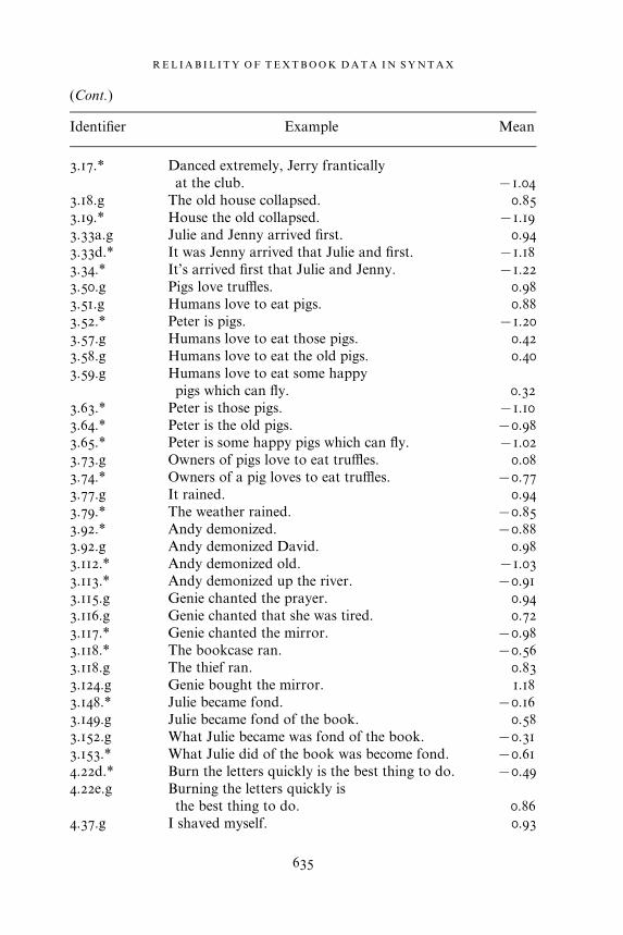
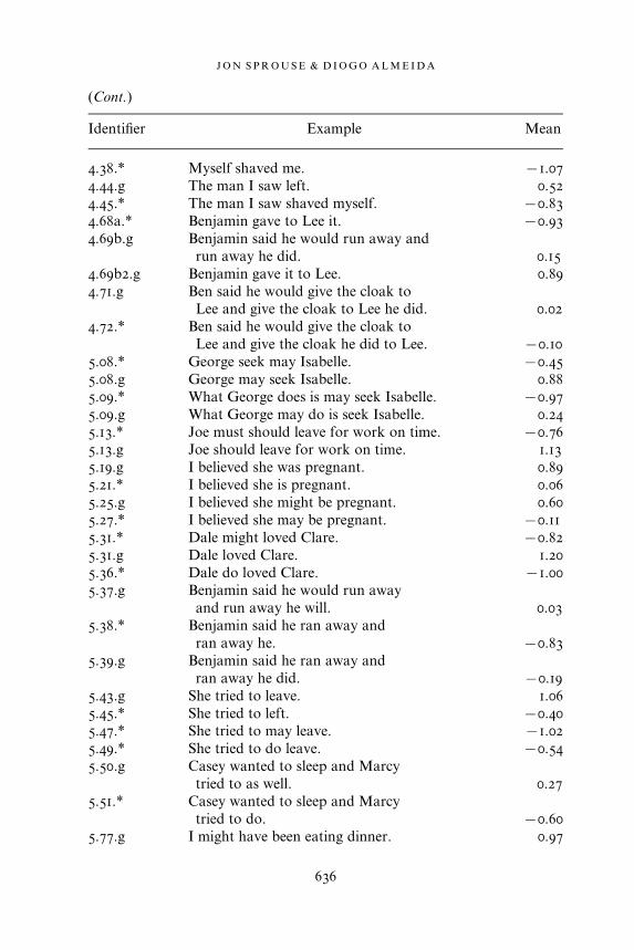
APPENDIX A
Example materials and mean ratings for
Experiment 1 (magnitude estimation)
Identifier Example Mean
2.01.g The pig grunts. 0.65
2.02.g The pigs grunt. 0.55
2.03.* The pig grunt. x0.81
2.04.* The pigs grunts. x0.26
2.53.* The scissors is lost. x0.71
2.53.g The scissors are lost. 1.01
2.68.g We all thought him to be unhappy. 0.36
2.69.g We all thought he was unhappy. 0.73
2.70.* We all thought he to be unhappy. x0.80
2.71.* We all thought him was unhappy. x0.83
2.81a.g The bears snuffled. 0.96
2.81b.* The bear snuffleds. x1.08
3.14.g At the club, Jerry danced
extremely frantically. 0.70
3.15.g Extremely frantically, Jerry
danced at the club. 0.13
3.16.* Frantically at, Jerry danced
extremely the club. x1.08
J O N S P R O U S E & D I O G O A L M E I D A
634
(Cont.)
Identifier Example Mean
3.17.* Danced extremely, Jerry frantically
at the club. x1.04
3.18.g The old house collapsed. 0.85
3.19.* House the old collapsed. x1.19
3.33a.g Julie and Jenny arrived first. 0.94
3.33d.* It was Jenny arrived that Julie and first. x1.18
3.34.* It’s arrived first that Julie and Jenny. x1.22
3.50.g Pigs love truffles. 0.98
3.51.g Humans love to eat pigs. 0.88
3.52.* Peter is pigs. x1.20
3.57.g Humans love to eat those pigs. 0.42
3.58.g Humans love to eat the old pigs. 0.40
3.59.g Humans love to eat some happy
pigs which can fly. 0.32
3.63.* Peter is those pigs. x1.10
3.64.* Peter is the old pigs. x0.98
3.65.* Peter is some happy pigs which can fly. x1.02
3.73.g Owners of pigs love to eat truffles. 0.08
3.74.* Owners of a pig loves to eat truffles. x0.77
3.77.g It rained. 0.94
3.79.* The weather rained. x0.85
3.92.* Andy demonized. x0.88
3.92.g Andy demonized David. 0.98
3.112.* Andy demonized old. x1.03
3.113.* Andy demonized up the river. x0.91
3.115.g Genie chanted the prayer. 0.94
3.116.g Genie chanted that she was tired. 0.72
3.117.* Genie chanted the mirror. x0.98
3.118.* The bookcase ran. x0.56
3.118.g The thief ran. 0.83
3.124.g Genie bought the mirror. 1.18
3.148.* Julie became fond. x0.16
3.149.g Julie became fond of the book. 0.58
3.152.g What Julie became was fond of the book. x0.31
3.153.* What Julie did of the book was become fond. x0.61
4.22d.* Burn the letters quickly is the best thing to do. x0.49
4.22e.g Burning the letters quickly is
the best thing to do. 0.86
4.37.g I shaved myself. 0.93
R E L I A B I L I T Y O F T E X T B O O K D A T A I N S Y N T A X
635
(Cont.)
Identifier Example Mean
4.38.* Myself shaved me. x1.07
4.44.g The man I saw left. 0.52
4.45.* The man I saw shaved myself. x0.83
4.68a.* Benjamin gave to Lee it. x0.93
4.69b.g Benjamin said he would run away and
run away he did. 0.15
4.69b2.g Benjamin gave it to Lee. 0.89
4.71.g Ben said he would give the cloak to
Lee and give the cloak to Lee he did. 0.02
4.72.* Ben said he would give the cloak to
Lee and give the cloak he did to Lee. x0.10
5.08.* George seek may Isabelle. x0.45
5.08.g George may seek Isabelle. 0.88
5.09.* What George does is may seek Isabelle. x0.97
5.09.g What George may do is seek Isabelle. 0.24
5.13.* Joe must should leave for work on time. x0.76
5.13.g Joe should leave for work on time. 1.13
5.19.g I believed she was pregnant. 0.89
5.21.* I believed she is pregnant. 0.06
5.25.g I believed she might be pregnant. 0.60
5.27.* I believed she may be pregnant. x0.11
5.31.* Dale might loved Clare. x0.82
5.31.g Dale loved Clare. 1.20
5.36.* Dale do loved Clare. x1.00
5.37.g Benjamin said he would run away
and run away he will. 0.03
5.38.* Benjamin said he ran away and
ran away he. x0.83
5.39.g Benjamin said he ran away and
ran away he did. x0.19
5.43.g She tried to leave. 1.06
5.45.* She tried to left. x0.40
5.47.* She tried to may leave. x1.02
5.49.* She tried to do leave. x0.54
5.50.g Casey wanted to sleep and Marcy
tried to as well. 0.27
5.51.* Casey wanted to sleep and Marcy
tried to do. x0.60
5.77.g I might have been eating dinner. 0.97
J O N S P R O U S E & D I O G O A L M E I D A
636

(Cont.)
Identifier Example Mean
5.81.* I have might be eating dinner. x0.76
5.84.* I’d planned to have finished, and
have finished I did. x0.68
5.84.g I’d planned to have finished, and
finished I have. x0.33
5.92.g Jason has been arguing with Noel. 0.93
5.93.* Jason is having argued with Noel. x0.69
5.133.* Ryan not flew the airplane. x1.19
5.135.g Ryan did not fly the airplane. 1.13
5.139.g Ryan has never flown an airplane. 1.06
5.140.* Ryan never has flown an airplane. 0.47
5.144.g Jason hasn’t arrived. 0.91
5.145.* Jason not arrived. x0.89
5.146.g Jason didn’t arrive. 1.00
5.147.* Jason didn’t arrived. 0.05
6.5.g All the horses had escaped. 0.66
6.7.g The horses had all escaped. 0.63
6.9–.* Horses have most been domesticated. x0.53
6.9.g Most horses have been domesticated. 1.11
6.38.g She has kissed her. 0.80
6.39.* Her has kissed her. x1.04
6.40.* She has kissed she. x1.03
6.45a.* There was he in the garden. x0.72
6.45b.* There was him in the garden. x0.81
6.45c.g There was a man in the garden. 1.10
6.58.* Him has he known. x0.97
6.58.g He has known him. 0.62
6.93.* The clothes were stole. x0.47
6.93.g The clothes were stolen. 0.76
6.98.g The boy was killed by Stan. 0.89
6.99.* The boy arrived by Stan. x0.53
6.100.* There arrived by Stan. x1.00
6.102.* There were killed three men by the assassin. x0.57
6.102.g Three men were killed by the assassin. 1.06
6.106.* Elliot quickly may free the animals. 0.06
6.107.g Elliot may quickly free the animals. 0.83
6.108.g Elliot could quickly have freed the animals. 0.39
6.112.* Garry failed often calculus exams. x0.63
6.112.g Garry often failed calculus exams. 0.99
R E L I A B I L I T Y O F T E X T B O O K D A T A I N S Y N T A X
637

(Cont.)
Identifier Example Mean
7.03.g The letters are on the table. 1.04
7.04.* Letters the are on the table. x0.96
7.06.g Letters are on the table. 1.07
7.07.* Letter is on the table. x0.09
7.30.* The this man needs a taxi. x0.30
7.30.g This man needs a taxi. 1.20
7.52.g Evan’s idea is brilliant. 1.07
7.53.* The Evan’s idea is brilliant. x0.51
7.54.* Evan’s the idea is brilliant. x0.90
7.89.* He analysis her was flawed. x1.02
7.90.g His analysis of her was flawed. 0.39
7.103.* A book of my is on the desk. x0.70
7.104.g A book of mine is on the desk. 0.58
7.105.* The therapist’s analysis of Morticia’s
was flawed. 0.13
7.105.g The therapist’s analysis of Morticia
was flawed. 0.83
8.03.* What she thought that was the poison
was neutralized. x0.51
8.03.g What she thought was that the poison
was neutralized. 0.18
8.05.g Everyone claimed that the wedding
was beautiful. 1.07
8.06.? That the wedding was beautiful was
claimed by everyone. x0.34
8.07.* The wedding was beautiful was
claimed that by everyone. x0.90
8.19.g Jason wondered whether the potion
was ready. 1.13
8.21.* Jason wondered whether that the
potion was ready. 0.19
8.23.g What Jason wondered was whether
the potion was ready. 0.31
8.24.* What Jason wondered whether was
the potion was ready. x0.57
8.29.* Jason wondered that the potion
was ready. x0.34
8.29.g Jason wondered whether the potion
was ready. 1.13
J O N S P R O U S E & D I O G O A L M E I D A
638

(Cont.)
Identifier Example Mean
8.56.g That the answer is obvious upset Helen. x0.10
8.57.* That that the world is round is obvious
upset Helen. x0.65
8.58.* That whether the world is round is
unknown upset Helen. x0.54
8.62.g That Jason had arrived annoyed Mandy. x0.05
8.64.* That Jason had arrived was obvious
annoyed Mandy. x0.60
8.65.* I said that that Jason had arrived
annoyed Mandy. x0.66
8.70.g There arrived a new actor on the set. 0.24
8.71.* The director arrived a new actor on the set. x0.73
8.74.g Laura tried to bathe her children. 0.99
8.76.* Laura tried Laura to bathe her children. x1.02
8.77.* Laura tried the babysitter to bathe
her children. x0.86
8.92.* We believed to be omnipotent. x0.81
8.93.g No one expected to win. 0.61
8.102.g Brian intended for him to learn magic. 0.86
8.103.* Brian intended for he to learn magic. x0.83
8.104.* Brian intended for to learn magic. x0.69
8.105.* For to do that would be a mistake. x0.57
8.105.g For him to do that would be a mistake. 0.53
8.120.g We believed him to be omnipotent. 0.55
8.131.g What Brian intended was for him to
learn magic. 0.48
8.132.g What Brian tried was to learn magic. 0.31
8.133.* What Brian believed was him to
be omnipotent. x0.65
8.150.* Melissa seems that is happy. x0.93
8.151.g It seems that Melissa is happy. 0.83
8.152.g Melissa seems to be happy. 1.00
8.166.g It stinks that Zeus is omnipotent. 0.95
8.167.* Zeus stinks to be omnipotent. x0.75
8.168.g There seems to be a man in the garden. 0.69
8.176.* There seems a man to be in the garden. x0.27
8.184.g I expected there to be a problem. 0.25
8.185.* I persuaded there to be a problem. x0.48
9.04.g Who did Nancy poison? 1.12
R E L I A B I L I T Y O F T E X T B O O K D A T A I N S Y N T A X
639

(Cont.)
Identifier Example Mean
9.12.* Someone did Nancy poison. x1.01
9.25.* Where place are you living? x0.64
9.28.g Which poem did Harry recite? 1.03
9.32.* Which the poem did Harry recite? x0.35
9.83.* I wondered could we leave early. 0.18
9.83.g I wondered if we could leave early. 1.03
9.84.* I wondered who did Nancy poison. x0.18
9.84.g I wondered who Nancy poisoned. 0.89
9.105.* Jason thinks who Nancy poisoned. x0.80
9.120.* Who did who poison? x0.54
9.120.g Who poisoned who? 0.11
9.122.g Who did Anna introduce to whom? 0.01
9.123.* Who did Anna introduce who to? x0.21
9.124.g Which poet wrote which poem? 0.40
9.125.g Which poem did which poet write? x0.10
10.55.g I asked who poisoned who? 0.27
10.56.* I asked who who poisoned? x0.91
10.58.* Who did you ask who poisoned? x0.90
10.69.g I believed the claim that Philip would
visit the city of Athens. 0.60
10.70.* Which city did you believe the claim
that Philip would visit? x0.43
10.71.g Peter listened to Darren’s speech about
investment banks. 1.07
10.72.* What did Peter listen to Darren’s
speech about? x0.45
10.73.g Penny was interested in Philip’s
description of geometry class. 0.95
10.74.* What was Penny interested in Philip’s
description of? x0.24
10.83.* What did Peter listen to those speeches
about? x0.30
10.84.g What did Peter listen to a speech about? 0.18
10.90.g That Peter loved Amber was obvious. 0.06
10.91.g It was obvious that Peter loved Amber. 1.02
10.92.g Who was it obvious that Peter loved? x0.39
10.93.* Who was that Peter loved obvious? x1.04
10.94.g That Peter loved Amber seemed to be
known by everyone. 0.05
J O N S P R O U S E & D I O G O A L M E I D A
640

(Cont.)
Identifier Example Mean
10.95.* Who did that Peter loved seem to be
known by everyone? x0.97
10.107a.g A program about Elephants is on
channel 4 tonight. 0.97
10.107b.* What is a program about on channel
4 tonight? x0.39
10.108a.g There is a program about Elephants on
channel 4 tonight. 1.02
10.108b.g What is there a program about on
channel 4 tonight? x0.04
10.116.g I worried after the lawyer forgot his
briefcase at the office. 0.58
10.117.g I worried because the lawyer forgot
his briefcase at the office. 0.73
10.118.g I worry if the lawyer forgets his
briefcase at the office. 0.18
10.119.* What did you worry after the lawyer
forgot at the office? x0.79
10.120.* What did you worry because the
lawyer forgot at the office? x0.73
10.121.* What do you worry if the lawyer
forgets at the office? x0.61
APPENDIX B
Materials and responses for Experiment 2 (yes–no)
Identifier Sentence Hits Trials
2.43.g She is shorter than he is. 25 39
2.45.g She is the shortest of the group! 25 40
2.82.g Mary will make spaghetti. 26 40
2.83.g Richard is going to chop some wood. 27 40
2.92.g He has been happy. 27 38
2.93.g I am being followed. 28 40
2.96.g I need to eat more vegetables. 29 40
2.97.g I want to eat macaroni. 29 39
2.98.g I must eat macaroni. 29 38
R E L I A B I L I T Y O F T E X T B O O K D A T A I N S Y N T A X
641

(Cont.)
Identifier Sentence Hits Trials
3.01.g That bottle of water might have
been cracked open. 29 37
3.02.g It might have cracked open. 32 39
3.05.g That one might have cracked open. 34 39
3.11.g This bottle of wine hasn’t gone bad,
but that bottle of wine might have. 31 40
3.12.g This bottle of wine won’t go bad,
but that bottle of wine might. 31 39
3.22.g It’s Alex that I like. 32 40
3.23.g It was under the bed that Lucy found
the missing watch. 32 40
3.24.g It was Julie and Jenny that arrived first. 32 38
3.25.g It was over the hill and through the
woods that they came running. 33 38
3.26.g I like Alex. 33 38
3.27.g Under the bed is the best place to hide. 33 40
3.28.g Julie and Jenny arrived first. 33 40
3.29.g They came running over the hill and
through the woods. 33 39
3.30d.g It’s Andy that I like. 33 38
3.32.g They arrived first. 33 40
3.35.g Matt didn’t pass the exam, but Julie
and Jenny did. 34 38
3.53.g Those pigs love truffles. 34 39
3.54.g The old pigs love truffles. 34 40
3.55.g Some happy drivers who own hybrid cars
can drive in carpool lanes. 34 40
3.56.g Some disgruntled old men in the post
office are complaining about postage rates. 35 38
3.81.g Alison ran. 35 40
3.82.g Alison joked. 35 40
3.83.g The horse galloped. 35 40
3.84.g Alison collapsed. 35 40
3.85.g Andy appeared suddenly. 35 40
3.86.g The horse fell during the race. 35 40
3.87.g Brian kicked the cat. 35 40
3.88.g Jenny swallowed the fly. 35 40
3.89.g Truman punched Johnson. 35 38
3.90.g Arthur gave the tapestry to Lancelot. 35 39
3.91.g The butler sent the letter to Dana. 35 40
J O N S P R O U S E & D I O G O A L M E I D A
642

(Cont.)
Identifier Sentence Hits Trials
3.97.g The landlord donated a helicopter. 36 40
3.98.g The students demonstrated the technique
this morning. 36 39
3.99.g I have eaten already. 36 40
3.100.g Julie felt hot. 30 39
3.101.g Julie felt he was there. 30 40
3.102.g Julie felt a twinge in her arm. 30 39
3.128.g He became fond of peanuts. 31 40
3.129.g He is unhappy about his contact-lenses. 32 38
4.06.g Please delete the emails from Peter ! 37 39
4.07.g Please delete the emails from him! 37 40
4.08.g Please delete them! 37 40
4.11.g Michael left Meg. 36 40
4.14.g Paul deleted the emails from Peter. 36 40
4.17.g Andy teased David every day. 36 40
4.18.g Shelly insulted Dana at the club. 36 40
4.19.g Martin complimented Tiffany almost
constantly. 36 39
4.22a.g Burn the letters quickly! 36 39
4.22b.g I burnt the letters quickly. 36 40
4.22c.g I plan to burn the letters quickly. 37 39
4.24.g Kiss Alex quickly ! 37 38
4.26.g Quickly kiss Angela! 37 40
4.28.g Julie quickly answered the question. 37 38
4.30.g Jenny poked Jonathan. 37 40
4.46.g The man I saw left. 37 39
4.47.g He left. 37 37
4.48.g You wanted to meet the man I saw. 37 38
4.49.g It was the man I saw that you wanted
to meet. 37 40
4.74.g The intrepid pirate and the fearful
captain’s mate sank the galleon. 37 38
4.75.g Sam hated the mean teacher and the
sarcastic principal. 37 39
4.76.g John hated the mean teacher and loved
the friendly principal. 37 38
4.77.g The very old and extremely wise teacher
announced her retirement. 37 39
4.88a.g Sam gave Lindsay the necklace. 37 40
4.88b.g Dan sent Nathan the binoculars. 37 39
R E L I A B I L I T Y O F T E X T B O O K D A T A I N S Y N T A X
643

(Cont.)
Identifier Sentence Hits Trials
4.88c.g Lee showed Benjamin the unicorn. 37 40
4.89a.g Benjamin gave the cloak to Lee. 37 38
4.89b.g Lucy sent the binoculars to Nathan. 37 38
4.89c.g Lee showed the unicorn to Benjamin. 38 40
4.90.g Benjamin gave Lee the book and Nathan
the magazine. 38 38
4.100a.g Emily caused Benjamin to see himself
in the mirror. 36 39
4.100b.g Benjamin caused Lee to catch a cold. 36 40
4.100c.g Phillip’s note caused Ryan to go to England. 36 39
4.101a.g Emily showed the baby himself in the mirror. 36 38
4.101b.g Benjamin gave Lee the book. 36 40
4.101c.g Benjamin sent the book to Ross. 36 39
5.03.g Greg may call Isabelle later. 38 38
5.04.g Greg must call Isabelle. 38 40
5.05.g Greg can call Isabelle later. 38 40
5.06.g Greg should call Isabelle later. 38 40
5.07.g Greg will call Isabelle. 38 38
5.32.g He couldn’t free the birds, but Andrew
did free the animals. 38 40
5.33.g Erica doesn’t rescue stray dogs, but he
does rescue stray cats. 38 39
5.34.g Dale rescued stray dogs. 38 39
5.35.g Erica rescues stray cats. 38 40
5.41.g Greg loved Isabelle and Eric did too. 38 38
5.42.g Terry fears snakes and Susan does as well. 38 40
5.61.g Jerry misses Erica. 38 38
5.62.g Jerry missed Eric. 38 39
5.76.g Erica misses Dan. 38 38
5.85.g I have eaten. 38 39
5.89.g Greg is kissing Sharon. 38 40
5.95.g I haven’t left yet. 38 38
5.97.g I was sitting not under the tree but
under the bush. 38 38
5.98.g I was eating not a peach but an apple. 38 40
5.99.g I might be not going to the party but
going to the movies instead. 38 40
5.100.g It is true that I might be doing something
other than going to the party. 38 38
5.101.g It is not true that I might be going to the party. 38 38
J O N S P R O U S E & D I O G O A L M E I D A
644

(Cont.)
Identifier Sentence Hits Trials
5.142.g George never drives motorcycles. 38 39
6.03.g Cassandra has foretold disaster again. 38 38
6.23.g The dinosaurs simply all died out. 38 38
6.24.g There are many fish in the sea. 38 38
6.25.g There were people playing on the beach. 38 38
6.26.g It’s quarter past four. 38 38
6.27.g It’s extremely windy today. 38 38
6.28.g I saw people playing there on the beach. 38 40
6.29.g Many fish are in the sea. 38 38
6.30.g People were playing on the beach. 38 40
6.33.g There’s going to be a party, isn’t there? 38 38
6.34.g There were people eating fire at the fair,
weren’t there? 38 39
6.69.g John arrives early on Sundays. 38 39
6.90a.g Mandy kissed Jason 38 38
6.90b.g Jason was killed. 38 39
6.104.g Tom quickly freed the animals. 38 39
6.117.g Perhaps Harry should be leaving. 38 38
6.118.g Fortunately Harry passed the exam. 38 38
6.119.g Ron failed the exam, unfortunately. 38 40
6.121.g Greg perhaps should be leaving. 38 39
6.122.g Billy fortunately has passed the exam. 38 38
7.02.g The letter was written by John. 39 39
7.05.g Those letters were supposed to be private. 39 39
7.8a.g The mailman lost the letters. 39 39
7.8b.g A letter is in the mail. 39 40
7.09.g Some letters should never be read. 39 39
7.10.g We asked some guy on the street for directions. 38 39
7.11.g Show me the emails ! 38 39
7.12.g This chair is made of metal. 38 40
7.13.g These chairs are reserved. 38 38
7.17.g I ate that. 39 39
7.18.g Every chair was taken. 39 40
7.19.g Nate folded up every chair. 39 40
7.20.g These expensive bottles of absinthe were
purchased at the wine shop. 39 40
7.21.g Those bottles of absinthe were purchased
at the wine shop, and these ones were
purchased at a bar. 39 40
7.27.g No child can resist ice cream. 39 40
R E L I A B I L I T Y O F T E X T B O O K D A T A I N S Y N T A X
645
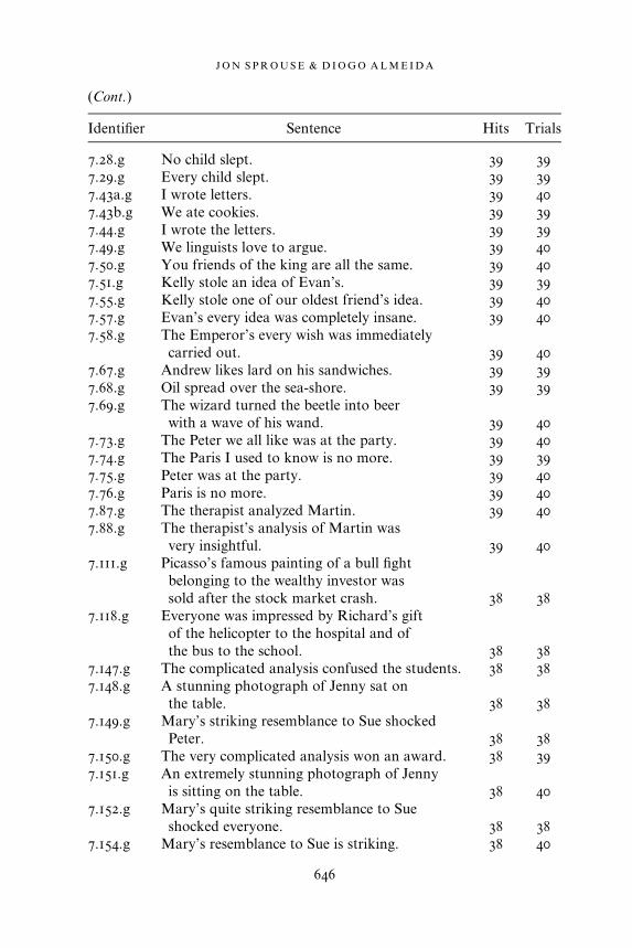
(Cont.)
Identifier Sentence Hits Trials
7.28.g No child slept. 39 39
7.29.g Every child slept. 39 39
7.43a.g I wrote letters. 39 40
7.43b.g We ate cookies. 39 39
7.44.g I wrote the letters. 39 39
7.49.g We linguists love to argue. 39 40
7.50.g You friends of the king are all the same. 39 40
7.51.g Kelly stole an idea of Evan’s. 39 39
7.55.g Kelly stole one of our oldest friend’s idea. 39 40
7.57.g Evan’s every idea was completely insane. 39 40
7.58.g The Emperor’s every wish was immediately
carried out. 39 40
7.67.g Andrew likes lard on his sandwiches. 39 39
7.68.g Oil spread over the sea-shore. 39 39
7.69.g The wizard turned the beetle into beer
with a wave of his wand. 39 40
7.73.g The Peter we all like was at the party. 39 40
7.74.g The Paris I used to know is no more. 39 39
7.75.g Peter was at the party. 39 40
7.76.g Paris is no more. 39 40
7.87.g The therapist analyzed Martin. 39 40
7.88.g The therapist’s analysis of Martin was
very insightful. 39 40
7.111.g Picasso’s famous painting of a bull fight
belonging to the wealthy investor was
sold after the stock market crash. 38 38
7.118.g Everyone was impressed by Richard’s gift
of the helicopter to the hospital and of
the bus to the school. 38 38
7.147.g The complicated analysis confused the students. 38 38
7.148.g A stunning photograph of Jenny sat on
the table. 38 38
7.149.g Mary’s striking resemblance to Sue shocked
Peter. 38 38
7.150.g The very complicated analysis won an award. 38 39
7.151.g An extremely stunning photograph of Jenny
is sitting on the table. 38 40
7.152.g Mary’s quite striking resemblance to Sue
shocked everyone. 38 38
7.154.g Mary’s resemblance to Sue is striking. 38 40
J O N S P R O U S E & D I O G O A L M E I D A
646

(Cont.)
Identifier Sentence Hits Trials
7.155.g Ben’s sleepy little rat ate some cheese. 38 40
7.156.g Kelly hated Jenny’s scraggly extremely
demonic cat. 38 39
7.157.g The dog in the yard howled loudly. 38 38
7.158.g Ron’s old sandwich in the refrigerator is
beginning to smell. 38 39
7.163.g Lucy’s disdain for Edmund was apparent
to everyone. 38 40
7.164.g The store clerk overheard our discussion
of porcupines. 38 40
7.166.g Ron heard a discussion in the foyer. 39 40
8.01.g I claimed she was pregnant 39 39
8.02.g I claimed that she was pregnant. 39 39
8.36.g Had the soup boiled over? 40 40
8.37.g Did the medicine work? 40 40
8.47.g That the waiter hates his job is obvious
to everyone. 40 40
8.48.g That the golden thread would show Jason his
path through the labyrinth was obvious. 40 40
8.49.g That I am here proves that I care. 40 40
8.50.g That Zeus was so promiscuous astounded the
other gods. 40 40
8.51.g That Susan kissed Brian didn’t surprise
anyone. 40 40
8.54.* Did that Sally punished her children
upset Jason? 40 40
8.55.* Has that we have arrived back at our starting
point proved that the world is round? 40 40
8.68.g Believing that the world is flat gives one
some solace. 40 40
8.81.g To steal hexes from witches would be
dangerous. 40 40
8.82.g If one were to steal hexes from witches,
then that would be dangerous. 40 40
8.83.g It is not a good idea to perjure oneself
in court ! 40 40
8.84.g The ancient Greeks believed Zeus to be
omnipotent. 40 40
8.85.g No one expected Carl to win. 40 40
R E L I A B I L I T Y O F T E X T B O O K D A T A I N S Y N T A X
647

(Cont.)
Identifier Sentence Hits Trials
8.86.g The ancient Greeks believed that Zeus
was omnipotent. 40 40
8.87.g No one expected that Laura would win. 40 40
8.90.g The ancient Greeks believed him to
be omnipotent. 40 40
8.91.g No one expected him to win. 40 40
8.94.g I intended for Jenny to be present. 40 40
8.95.g For you to do that would be a mistake. 40 40
8.126.g Andy believed the report. 39 40
8.127.g Ron expected a pop quiz. 39 40
8.141.g It seems that Carl is a maniac. 39 40
8.142.g It appears that Victor owns a car. 39 40
8.143.g Carl seems to be a maniac. 39 40
8.144.g Helen appears to own a car. 39 40
8.163.g Sarah turned out to seem to be untrustworthy. 39 40
8.164.g Jason happens to appear to be wealthy. 39 40
8.177.g Jason persuaded Mike to visit his family. 39 39
8.178.g David forced Rita to leave the school. 39 40
8.193.g Jason persuaded Marcy that she should
visit her family. 39 39
8.199.g Before the police arrived, Sally had escaped. 39 40
8.200.g When the pizza arrived, Sally was asleep. 39 40
8.201.g After the police left, Helen wept. 39 39
8.202.g Harry had escaped, before the police arrived. 39 40
8.203.g Sally was asleep, when the pizza arrived. 39 39
8.204.g Helen wept, after the police left. 39 40
8.205.g Nancy thought that, after the police had left,
Sandy would be relieved. 39 39
8.208.g Judy was happy, because she had got the
highest grade in the class. 40 40
8.209.g Because she had got the highest grade in
the class, Mandy was happy. 40 40
8.210.g Jason became invisible, so that he could escape. 40 40
8.211.g So that he could escape, Jason became invisible. 40 40
8.224.g I think Coke is ok, but Pepsi, I can’t stand! 40 40
8.225.g I never liked his analysis. 40 40
9.06.g I asked who Michael liked. 40 40
9.07.g I asked if Michael liked Jason. 40 40
9.13.g What have you eaten? 40 40
9.14.g When did you arrive? 40 40
J O N S P R O U S E & D I O G O A L M E I D A
648

(Cont.)
Identifier Sentence Hits Trials
9.15.g Where are you living? 40 40
9.16.g Which book are you reading? 40 40
9.17.g Why are you leaving? 40 40
9.18.g How are you feeling? 40 40
9.30.g Homer recited the poem about Achilles. 40 40
9.31.g He is that kind of actor. 40 40
9.35.g How fond of Clara is Arnold? 40 40
9.36.g How quickly did the Greeks take Troy? 40 40
9.59.g Who ordered what? 40 40
9.60.g Who showed what to who? 40 40
9.72.g Who did you introduce Maria to? 40 40
9.73.g Why did you kill the spider? 40 40
9.74.g Where did Peter see George? 40 40
9.86.g Who has read the novel? 40 40
9.87.g Which teacher might help us? 40 40
9.88.g Who is sailing to Bermuda? 40 40
9.90.g Who read the novel? 40 40
9.91.g Which waiter served us? 40 40
9.101.g Who did Jason think that Mandy had poisoned? 40 40
9.102.g What did you say that the poet had written? 40 40
10.50.* Who seemed that had poisoned Jason? 21 40
REFERENCES
Adger, David. 2003. Core syntax: A Minimalist approach. Oxford: Oxford University Press.Alexopoulou, Theodora & Frank Keller. 2007. Locality, cyclicity and resumption: At the
interface between the grammar and the human sentence processor. Language 83, 110–160.Baayen, R. Harald. 2007. Analyzing linguistic data: A practical introduction to statistics using R.
Cambridge: Cambridge University Press.Baayen, R. Harald, Douglas J. Davidson & Douglas M. Bates. 2008. Mixed-effects modeling
with crossed random effects for subjects and items. Journal of Memory and Language 59,390–412.
Bader, Marcus & Jana Haussler. 2010. Toward a model of grammaticality judgments. Journal ofLinguistics 46, 273–330.
Bard, Ellen G., Dan Robertson & Antonella Sorace. 1996. Magnitude estimation of linguisticacceptability. Language 72, 32–68.
Chomsky, Noam. 1955/1957. The logical structure of linguistic theory. New York: PlenumPress.
Chomsky, Noam. 1965. Aspects of the theory of syntax. Cambridge, MA: MIT Press.Chomsky, Noam. 1986. Barriers. Cambridge, MA: MIT Press.Cohen, Jacob. 1962. The statistical power of abnormal social psychological research: A review.
Journal of Abnormal and Social Psychology 65, 145–153.
R E L I A B I L I T Y O F T E X T B O O K D A T A I N S Y N T A X
649

Cohen, Jacob. 1988. Statistical power analysis for the behavioral sciences, 2nd edn. Hillsdale, NJ:Erlbaum.
Cohen, Jacob. 1992. Statistical power analysis. Current Directions in Psychological Science 1,98–101.
Cowart, Wayne. 1997. Experimental syntax: Applying objective methods to sentence judgments.Thousand Oaks, CA: Sage.
Culbertson, Jennifer & Steven Gross. 2009. Are linguists better subjects? British Journal for thePhilosophy of Science 60, 721–736.
Culicover, Peter W. & Ray Jackendoff. 2010. Quantitative methods alone are not enough:Response to Gibson & Fedorenko. Trends in Cognitive Sciences 14, 234–235.
Dabrowska, Ewa. 2010. Naıve v. expert intuitions: An empirical study of acceptabilityjudgments. The Linguistic Review 27, 1–23.
den Dikken, Marcel, Judy Bernstein, Christina Tortora & Rafaella Zanuttini. 2007. Data andgrammar: Means and individuals. Theoretical Linguistics 33, 335–352.
Edelman, Shimon & Morten Christiansen. 2003. How seriously should we take Minimalistsyntax? Trends in Cognitive Sciences 7, 60–61.
Fanselow, Gisbert. 2007. Carrots – perfect as vegetables, but please not as a main dish.Theoretical Linguistics 33, 353–367.
Featherston, Sam. 2005a. Magnitude estimation and what it can do for your syntax: Somewh-constraints in German. Lingua 115, 1525–1550.
Featherston, Sam. 2005b. Universals and grammaticality: Wh-constraints in German andEnglish. Linguistics 43, 667–711.
Featherston, Sam. 2007. Data in generative grammar: The stick and the carrot. TheoreticalLinguistics 33, 269–318.
Featherston, Sam. 2008. Thermometer judgments as linguistic evidence. In ClaudiaMaria Riehl & Astrid Rothe (eds.), Was ist linguistische evidenz?, 69–90. Aachen: ShakerVerlag.
Featherston, Sam. 2009. Relax, lean back, and be a linguist. Zeitschrift fur Sprachwissenschaft28, 127–132.
Ferreira, Fernanda. 2005. Psycholinguistics, formal grammars, and cognitive science. TheLinguistic Review 22, 365–380.
Gallistel, Randy. 2009. The importance of proving the null. Psychological Review 116, 439–53.Gibson, Edward. 1991. A computational theory of human linguistic processing:
Memory limitations and processing breakdown. Ph.D. dissertation, Carnegie MellonUniversity.
Gibson, Edward & Evelina Fedorenko. 2010. Weak quantitative standards in linguisticsresearch. Trends in Cognitive Sciences 14, 233–234.
Gibson, Edward & Evelina Fedorenko. In press. The need for quantitative methods in syntaxand semantics research. Language and Cognitive Processes, doi :10.1080/01690965.2010.515080.Published online by Taylor & Francis, 4 May 2011.
Gibson, Edward, Steve Piantadosi & Kristina Fedorenko. 2011. Using Mechanical Turk toobtain and analyze English acceptability judgments. Language and Linguistics Compass 5,509–524.
Grewendorf, Gunter. 2007. Empirical evidence and theoretical reasoning in generative grammar.Theoretical Linguistics 33, 369–381.
Gross, Steven & Jennifer Culbertson. 2011. Revisited linguistic intuitions. British Journal for thePhilosophy of Science 62, 639–656.
Haider, Hubert. 2007. As a matter of facts – comments on Featherston’s sticks and carrots.Theoretical Linguistics 33, 381–395.
Hill, Archibald A. 1961. Grammaticality. Word 17, 1–10.Hofmeister, Philip, T. Florian Jaeger, Inbal Arnon, Ivan A. Sag & Neal Snider. In press. The
source ambiguity problem: Distinguishing the effects of grammar and processing on ac-ceptability judgments. Language and Cognitive Processes, doi : 10.1080/01690965.2011.572401.Published online by Taylor & Francis, 18 October 2011.
Jeffreys, Harold. 1961. Theory of probability. Oxford: Oxford University Press.Kayne, Richard S. 1983. Connectedness. Linguistic Inquiry 14, 223–249.Keller, Frank. 2000. Gradience in grammar: Experimental and computational aspects of degrees
of grammaticality. PhD. dissertation, University of Edinburgh.
J O N S P R O U S E & D I O G O A L M E I D A
650

Keller, Frank. 2003. A psychophysical law for linguistic judgments. In Richard Alterman &David Kirsh (eds.), The 25th Annual Conference of the Cognitive Science Society, 652–657.Boston.
Myers, James. 2009. Syntactic judgment experiments. Language and Linguistics Compass 3,406–423.
Newmeyer, Frederick J. 2007. Commentary on Sam Featherston, ‘Data in generative grammar:The stick and the carrot’. Theoretical Linguistics 33, 395–399.
Nickerson, Raymond. 2000. Null hypothesis significance testing: A review of an old andcontinuing controversy. Psychological Methods 5, 241–301.
Pesetsky, David. 1987. WH-in-situ: Movement and unselective binding. In Eric Reuland &Alice G. B. ter Meulen (eds.), The linguistic representation of (in)definiteness, 98–129.Cambridge, MA: MIT Press.
Phillips, Colin. 2009. Should we impeach armchair linguists? In Shoishi Iwasaki, Hajime Hoji,Patricia Clancy & Sung-Ock Sohn (eds.), Japanese/Korean Linguistics 17. Stanford, CA: CSLIPublications.
Phillips, Colin & Howard Lasnik. 2003. Linguistics and empirical evidence: Reply to Edelmanand Christiansen. Trends in Cognitive Sciences 7, 61–62.
Rouder, Jeffrey N., Paul L. Speckman, Dongchu Sun, Richard D. Morey & Geoffrey Iverson.2009. Bayesian t-tests for accepting and rejecting the null hypothesis. Psychonomic Bulletin &Review 16, 225–237.
Schutze, Carson. 1996. The empirical base of linguistics: Grammaticality judgments and linguisticmethodology. Chicago: University of Chicago Press.
Schutze, Carson & Jon Sprouse. In press. Judgment data. In Devyani Sharma &Rob Podesva (eds.), Research methods in linguistics. Cambridge: Cambridge UniversityPress.
Sorace, Antonella & Frank Keller. 2005. Gradience in linguistic data. Lingua 115, 1497–1524.Spencer, N. J. 1973. Differences between linguists and nonlinguists in intuitions of grammati-
cality-acceptability. Journal of Psycholinguistic Research 2, 83–98.Sprouse, Jon. 2007a. A program for experimental syntax. Ph.D. dissertation, University of
Maryland.Sprouse, Jon. 2007b. Continuous acceptability, categorical grammaticality, and experimental
syntax. Biolinguistics 1, 118–129.Sprouse, Jon. 2008. The differential sensitivity of acceptability to processing effects. Linguistic
Inquiry 39, 686–694.Sprouse, Jon. 2009. Revisiting satiation: Evidence for an equalization response strategy.
Linguistic Inquiry 40, 329–341.Sprouse, Jon. 2011a. A validation of Amazon Mechanical Turk for the collection of acceptability
judgments in linguistic theory. Behavior Research Methods 43, 155–167.Sprouse, Jon. 2011b. A test of the cognitive assumptions of Magnitude Estimation:
Commutativity does not hold for acceptability judgments. Language 87, 274–288.Sprouse, Jon & Diogo Almeida. 2012. The role of experimental syntax in an integrated
cognitive science of language. In Kleanthes Grohmann & Cedric Boeckx (eds.), TheCambridge handbook of biolinguistics. Cambridge: Cambridge University Press.
Sprouse, Jon & Diogo Almeida. 2011. Power in acceptability judgment experiments and thereliability of data in syntax. Ms., University of California, Irvine & Michigan State University.
Sprouse, Jon, Shin Fukuda, Hajime Ono & Robert Kluender. 2011. Grammatical operations,parsing processes, and the nature of wh-dependencies in English and Japanese. Syntax 14,179–203.
Sprouse, Jon, Carson Schutze & Diogo Almeida. 2011. Assessing the reliability of journal datain syntax: Linguistic Inquiry 2001–2010. Ms., University of California, Irvine; University ofCalifornia, Los Angeles & Michigan State University.
Sprouse, Jon, Matt Wagers & Colin Phillips. 2012. A test of the relation between workingmemory capacity and island effects. Language 88.1.
Stevens, Stanley Smith. 1957. On the psychophysical law. Psychological Review 64, 153–181.Wasow, Thomas & Jennifer Arnold. 2005. Intuitions in linguistic argumentation. Lingua 115,
1481–1496.Weskott, Thomas & Gisbert Fanselow. 2011. On the informativity of different measures of
linguistic acceptability. Language 87, 249–273.
R E L I A B I L I T Y O F T E X T B O O K D A T A I N S Y N T A X
651

Wetzels, Ruud, Jeroen G. W. Raaijmakers, Emoke Jakab & Eric-Jan Wagenmakers.2009. How to quantify support for and against the null hypothesis : A flexibleWinBUGS implementation of a default Bayesian t-test. Psychonomic Bulletin & Review16, 752–760.
Authors’ addresses : (Sprouse)Department of Cognitive Sciences, University of California,3151 Social Science Plaza A, Irvine, CA 92697-5100, [email protected]
(Almeida)Department of Linguistics and Languages,Michigan State University, A-621 Wells Hall,East Lansing, MI 48824-1027, [email protected]
J O N S P R O U S E & D I O G O A L M E I D A
652