assessing the impact of the jepara furniture value … jepara small-scale furniture producer...

Assessing the Impact of the Jepara Furniture Value Chain Project

Corinna Clements

Thesis submitted to the faculty of the Virginia Polytechnic Institute and State University

in partial fulfillment of the requirements for the degree of

Master of Science

In

Agricultural and Applied Economics

Jeffrey R. Alwang, Committee Chair

Daniel Suryadarma

Bradford F. Mills

July 25, 2016

Blacksburg, VA

Keywords:

propensity score matching, value chain, furniture, producer association, Indonesia

ii

Assessing the Impact of the Jepara Furniture Value Chain Project

Corinna Clements

ABSTRACT

This thesis assesses the impact of the Jepara Furniture Value Chain (FVC) project, which

was conducted by the Center for International Forestry Research (CIFOR) to address

challenges faced by small-scale furniture producers in Jepara, Indonesia. This assessment

focuses on the effect of membership in the APKJ, a producer association started as part of

the project. The propensity score for association membership was estimated using

unchanging firm and owner characteristics, as well as information recalled about firm

operations in 2009 (before the association was formed). Propensity score matching was

used to compare outcome variables of association members and non-members. Results

suggest that membership in the APKJ does not have a significant effect on profit levels.

Using differenced current and recalled marketing and production behaviors as outcome

variables with propensity score matching indicates that members have improved their

bargaining position and marketing behaviors more than non-members since 2009.

Additionally, APKJ members are more likely to have obtained certificates of timber

legality

iii

Acknowledgements

I would like to thank the Standing Panel on Impact Assessment of the CGIAR consortium

for funding this research through the project titled Strengthening Impact Assessment in

the CGIAR: New partnerships for building impact. Many thanks go to the Center for

International Forestry Research (CIFOR) for the opportunity to work with researchers at

CIFOR to conduct this research, and for supporting survey administration.

I would like to express my deep appreciation for my advisor and committee chair, Dr.

Jeff Alwang, for patiently guiding me through research and writing while challenging me

to think creatively and critically. You always invested the time to provide the feedback

that allowed me to learn and improve, and for that I am very grateful. I want to thank my

committee member Dr. Brad Mills. Your advice on surveying and propensity score

matching was immensely helpful. . Also thanks to Dr. Wen You for guidance on

propensity score matching. I am very thankful for the input that Dr. Daniel Suryadarma

provided on sample selection and the many iterations of the questionnaire. Thank you for

guiding me through preparing for survey administration and for making me feel welcome

at CIFOR.

I cannot thank Ramadhani Achdiawan enough for his essential role in developing and

testing the questionnaire, recruiting and training enumerators, and overseeing survey

administration. I also want to thank Sulthon M. Amin for recruiting enumerators from

Jepara, teaching me about furniture making and the APKJ, and assisting in overseeing

survey administration. I want to thank all of my enumerators, Vivi, Finanda, Ruli, Sorif,

Sinung, Arfan, Karwadi, and Nonik, and in particular Muhamad Risman and Rohazim

Anambas, who helped with translations and data entry in addition to interviewing. Thank

you to all of you; I greatly appreciate your hard work, and value your friendship. I also

want to thank Ibu Elfy for welcoming me into Situ Gede and making me feel at home.

I would also like to thank all my friends, particularly Brittany Castle, Kristen Clermont,

Lauren Pichon, Lauren Garcia, Stephanie Myrick and Bryan Lehner for reminding me to

have perspective and for listening to me ramble about topics such as calipers and

covariate balance. I am immensely grateful to my family for their constant support,

especially my Mom. Thank you for always being there for me, for calming me when I

was anxious, and for persistently believing in me.

iv

Table of Contents

ABSTRACT .................................................................................................................................... ii

Acknowledgements ........................................................................................................................ iii

Table of Contents ........................................................................................................................... iv

Chapter 1: Introduction ................................................................................................................... 1

1.1 Problem Statement and Objectives ....................................................................................... 1

1.2 Methods and Hypotheses ...................................................................................................... 3

1.3 Overview of thesis ................................................................................................................ 5

Chapter 2: Background ................................................................................................................... 6

2.1 The Jepara Furniture Value Chain Project ............................................................................ 6

2.2 The Jepara Furniture Value Chain ........................................................................................ 7

2.3: Project implementation ...................................................................................................... 13

Chapter 3: Methods ....................................................................................................................... 17

3.1 Conceptual Framework and Empirical Model .................................................................... 17

3.2 Data Collection and the Survey Instrument ........................................................................ 22

3.2.1 The Survey Instrument ................................................................................................. 24

3.2.2 Sample Selection .......................................................................................................... 25

3.3 Data ..................................................................................................................................... 28

3.3.1 Comparing recall responses with data from previous survey ...................................... 28

3.3.1 Covariates .................................................................................................................... 29

3.3.2 Outcome Variables....................................................................................................... 40

Chapter 4: Analysis and Results ................................................................................................... 45

4.1: Implementing Empirical Methods ..................................................................................... 45

4.2: Checking Common Support and Covariate Balance Assumptions ................................... 47

4.3: Hypotheses and Results ..................................................................................................... 51

4.3.1: Hypothesis 1: APKJ members realize higher profits than non-members with similar

attributes ................................................................................................................................ 51

4.3.2: Hypothesis 2: APKJ members have a higher probability than non-members of

increasing the sophistication of their marketing methods between 2009 and 2015 ............. 57

4.3.3: Hypothesis 3: APKJ members are more likely than non-members to have upgraded

their production activities since 2009 ................................................................................... 65

4.3.4: Hypothesis 4: APKJ members are more likely than non-members to have good

business management practices ............................................................................................ 67

4.3.5: Revenue Predictors and Staying Open versus Shutting Down ................................... 69

4.4: Qualitative Survey Responses ........................................................................................... 72

4.5: Conclusion and Limitations ............................................................................................... 73

Chapter 5: Discussion ................................................................................................................... 75

References ..................................................................................................................................... 79

v

Appendix A: Survey Questionnaire .............................................................................................. 82

Appendix B: Balance Tests ......................................................................................................... 108

Appendix C: Stata Code.............................................................................................................. 110

Appendix D: Treatment Effects for Matching Without Replacement ........................................ 154

Appendix E: Institutional Review Board Approval Letter ......................................................... 157

List of Tables

Table 1: Selection of Respondents Based on Wood Products and Firm Scale ............................. 27

Table 2: Descriptions of covariates in propensity score calculation ............................................. 29

Table 3: Variables used in creation of woodworking equipment index ....................................... 34

Table 4: Business unit ownership of APKJ members and control respondents before matching 36

Table 5: Sub-district representation in current and past surveys .................................................. 39

Table 6: Seasonality table from 2015 firm survey questionnaire ................................................. 42

Table 7: Descriptive statistics of estimated profit in treatment and control groups ..................... 52

Table 8: Average treatment effect on the treated for estimated firm profit (matching with

replacement) .................................................................................................................................. 54

Table 9:Average treatment effect on the treated for estimated firm profit (matching with

replacement) .................................................................................................................................. 57

Table 10: Tabulated data, treatment effects, and risk ratios for changes in the practice of

marketing through exhibitions (2009-2015) ................................................................................. 58

Table 11: Tabulated data, treatment effects, and risk ratios for changes in practice of selling

directly to buyers (2009-2015) ...................................................................................................... 60

Table 12: Tabulated data, treatment effects, and risk ratios for changes in use of practice of

online marketing (2009-2015) ...................................................................................................... 60

Table 13: Tabulated data, treatment effects, and risk ratios for changes in practice of exporting

furniture (2009-2015).................................................................................................................... 62


through other showrooms (2009-2015) ........................................................................................ 63


through (to) brokers (2009-2015) ................................................................................................. 64

Table 16: Tabulated data, treatment effects, and risk ratios for changes in practice of being

subcontracted (2009-2015) ........................................................................................................... 64

Table 17: Tabulated data, treatment effects, and risk ratios for changes in brokering status 2009-

2015............................................................................................................................................... 66

Table 18: Tabulated data, treatment effects, and risk ratios for changes in selling finished

products 2009-2015 ...................................................................................................................... 66

Table 19: Tabulated data, treatment effects, and risk ratios for SVLK certification .................... 68

Table 20: Tabulated data, treatment effects, and risk ratios for record-keeping .......................... 69

Table 21: Tabulated data, treatment effects, and risk ratios for business registration .................. 69

Table 22: Ordinary least square estimates for predictors of firm revenues .................................. 70

Table 23: Tabulated data, treatment effects, and risk ratios for businesses closing ..................... 72

Table 24: Member-identified benefits of the APKJ ...................................................................... 73

vi

List of Figures

Figure 1: Map of Jepara .................................................................................................................. 8

Figure 2: Jepara Furniture Value Chain .......................................................................................... 9

Figure 3: Common support when matching to one nearest neighbor without a caliper ............... 48

Figure 4: Kernel density of estimated profit for members and non-members before matching ... 52

Figure 5: Kernel density of estimated profit after caliper matching to one nearest neighbor ...... 53

Figure 6: Kernel density of estimated profit of full sample .......................................................... 55

Figure 7: Kernel density of estimated revenues after caliper matching to one nearest neighbor . 56

1

Chapter 1: Introduction

1.1 Problem Statement and Objectives

The wooden furniture industry of Jepara, Indonesia is central to the District’s economy.

Teak and mahogany carving has been culturally and economically important to the region for

hundreds of years. The industry grew between 1997 and 2005, but declined after the financial

crisis of 2008 (Loebis and Schmitz, 2005, Achdiawan and Purnomo, 2010, Purnomo et al.,

2014).Today, it contributes an estimated 26% to Jepara’s GDP (Melati et al., 2013). In 2010, the

industry was composed of 11, 357 business units, the vast majority of which were small in scale

(Achdiawan and Purnomo, 2010, Melati et al., 2013). The industry as a whole is confronted by

increasing scarcity of timber, international pressures for assurance of timber legality, and

increased international competition (Loebis and Schmitz, 2005). Small-scale producers are

particularly vulnerable to industry pressures. In addition, small-scale producers suffer from

limited bargaining power, inadequate access to credit, restricted market access, and insufficient

knowledge infusion (Purnomo et al., 2013a).

The Jepara Furniture Value Chain (FVC) project, conducted by the Center for

International Forestry Research (CIFOR) from 2008 to 2013, sought to address challenges faced

by small-scale furniture producers in Jepara. The objectives of the project were: “(i). to enhance

the structure and function of the furniture industry for the benefit of small-scale furniture

producers; (ii). To improve marketing by small-scale furniture producers and their industry

associations, and (iii). to monitor changes regarding the effects and early acceptance of

innovations from objectives 1 and 2 and revise and/or reinforce project strategies accordingly”

(Purnomo et al., 2013b).

These objectives were pursued based on the value chain upgrading approach, which

harnesses value chain analysis to develop a strategy for market system change (Herr and Muzira,

2

2009). Value chain analysis methodically evaluates the system that is comprised of the full range

of activities that carries a product or service from conception to the final consumer (Herr and

Muzira, 2009). By characterizing the relationships, incentives, and capacities of actors within the

value chain, the analysis brings about an understanding of systemic constraints. Identification of

these constraints allows for policy-makers and project-implementers to facilitate upgrading,

which consists of changes in the industry that improve firms’ competitiveness by improving the

efficiency of their current operations or adopting new production activities (Humphrey and

Schmitz, 2002).

Researchers in the Jepara Furniture Value Chain project initiated four such strategies for

upgrading in the Jepara Furniture Value Chain, or ‘upgrading scenarios,’ in Jepara: moving up,

collaborating down, green certification, and producer association. The last scenario, formation of

the Jepara Small-Scale Furniture Producer Association, or APKJ, facilitated implementation of

the three other upgrading scenarios by bringing together stakeholders for collective bargaining

power, improved marketing, and human resource development (Purnomo et al., 2013b). Producer

association members, of which there are currently 125, were the primary project participants.

Although CIFOR’s direct involvement ceased in 2013, the APKJ still exists, and policy

developments promoted by the project are in the process of being formalized into law. Project

stakeholders desire information about its impact: donors desire objective information on the

effects of the project, and project implementers seek feedback in order to guide the formation of

future projects. Researchers at CIFOR are hoping to implement a similar project in another

furniture cluster, making the results of the impact assessment immediately relevant (personal

communication with Herry Purnomo May 29, 2015). Determining the impacts of the APKJ will

indicate what impacts can be expected from policy implementation and from future projects.

3

The overarching objective of this research is to determine the impact of membership in

the APKJ. Sub-objectives which will contribute to fulfilling this objective are:

1. Quantify the livelihood impact of the project by comparing firm profits of APKJ

members against a counterfactual

2. Determine the extent of the uptake of upgrading behaviors promoted by the four

upgrading scenarios of the Jepara FVC project

3. Measure the effect of specific upgrading behaviors on revenues and profits

1.2 Methods and Hypotheses

The purpose of this research is to evaluate the impact of the Jepara FVC project,

providing feedback on the value of research investment and guiding the formation of future

projects. Impact assessment examines long-term sustainable changes that have been produced by

the project (Herr et al. 2006). Unlike other forms of monitoring and evaluation, impact

assessment hinges on accurately attributing results to project interventions. This requires

comparing outcome measures of project participants to what these measures would have been

absent project interventions (Khandker et al., 2010). Since it is impossible to know the outcome

at a given period of time for an individual in both the treated and untreated states, a valid

counterfactual must be created through thoughtful data collection and statistical analysis. For this

study, propensity score matching (PSM) will be used. PSM statistically constructs a valid control

group by first determining the probability of treatment for every treated and non-treated

individual (Khandker et al., 2010).

Calculation of the propensity score involves regressing pre-intervention or inherent (time-

invariant) characteristics of individuals (from both the treated and non-treated groups) on a

binary dependent variable representing treatment (in this case, membership in the producer

group). Data on outcome variables and matching characteristics were gathered in a 2015 firm

4

survey with 600 respondents. Both inherent and pre-intervention characteristics will be used to

calculate the propensity score. In order to achieve this, the survey questionnaire gathered

information on firm operations in 2009. These pre-treatment characteristics will be used as

variables to calculate the propensity score. To test hypotheses, APKJ members will be matched

with non-members with a similar propensity score. The propensity score will be calculated using

characteristics of the firm owner, firm characteristics, and firm operations in 2009. Hypotheses

will be tested by comparing levels of outcome variables for member and control units that have

been matched based on their propensity score.

Hypothesis 1: APKJ members realize higher profits than non-members with similar

attributes

Benefits from any upgrading undertaken by a firm is predicted to be captured by an

increase in profit. Therefore, profit is used as the primary outcome of interest. The survey

instrument focused on capturing information about costs and revenues in order to estimate firm

profit. Further detail about profit estimation is provided in chapter three.

Hypothesis 2: APKJ members have a higher probability than non-members with similar

attributes of increasing the sophistication of their marketing methods since 2009.

This hypothesis will be tested by comparing marketing methods in 2009 with marketing

methods in 2015. If a firm has increased the sophistication of its marketing activities then it will

have added new approaches to the marketing strategy. In particular, using an online marketing

platform and meeting buyers through exhibitions represent more sophisticated marketing

methods. Current marketing methods will be compared against recalled 2009 marketing

methods. This examines the effectiveness of the moving-up scenario.

Hypothesis 3: APKJ members are more likely than non-members with similar attributes to

have upgraded their production activities since 2009.

5

Firms can upgrade their production by creating a higher-value product through finishing

furniture, and improving their position in the value chain or by integrating high-returns upstream

activities such as marketing and brokering and shifting from being subcontracted to selling

directly to buyers. Recall and current data will be used to compare changes in matched units and

in total treatment and control groups. This measures the effectiveness of the moving-up scenario

and the green certification scenario.

Hypothesis 4: APKJ members are more likely than non-members to have good business

management practices.

Good management practices include keeping business records, obtaining SVLK

certification and having formally registered firms. This hypothesis will be tested by comparing

current levels of these practices of matched APKJ members and control units.

1.3 Overview of thesis

Chapter two of this thesis will provide detailed background information on the Jepara

furniture industry, value chain upgrading, and the Jepara Furniture Value Chain Project.

Examining the ways in which the Jepara Furniture Value Chain Project attempted to promote

value chain upgrading informed selection of outcome variables. The background provided in

chapter two provides context for understanding hypotheses and interpreting results. Chapter three

transitions to the details of this study. Propensity score matching is explained in further detail in

the conceptual framework and empirical methods section. A description of data collection

includes information on both sample selection and the survey instrument. Chapter three also

describes the covariates included in propensity score estimation as well as the outcome variables

used in the analysis. Following this, chapter four provides further detail about implementing the

empirical methods, and reports results of testing the hypotheses listed above. Chapter five

discusses the findings and implications of this study.

6

Chapter 2: Background This chapter provides background information to contextualize the current study. First, an

overview of the Jepara Furniture Value Chain Project is provided. Next, details are provided on

the Jepara furniture value chain, informed by research conducted as part of the Jepara Furniture

Value Chain Project. Following this, the actions that the project took to improve the livelihoods

and market position of producers are described.

2.1 The Jepara Furniture Value Chain Project

This study evaluates the impact of the Jepara Furniture Value Chain Project. The project

began in August 2008 as a collaboration between the Center for International Forestry Research,

the Forestry Research and Development Agency of the Indonesian Ministry of Forestry, and the

Faculty of Forestry of Bogor Agricultural University. It built upon an EU-funded project titled

“Levelling the Playing Field”, which was conducted 2003–2007. Value chain analysis and other

research conducted as part of this project informed the Jepara FVC Project, the objectives of

which were: “(i). to enhance the structure and function of the furniture industry for the benefit of

small-scale furniture producers; (ii). to improve marketing by small-scale furniture producers and

their industry associations, and (iii). to monitor changes regarding the effects and early

acceptance of innovations from objectives 1 and 2 and revise and/or reinforce project strategies

accordingly” (Purnomo et al., 2013).

The project began by conducting value chain analysis (VCA) and participatory action

research (PAR) in order to first identify stakeholders and constraints, and then involve

stakeholders in an iterative process of addressing constraints. PAR is implemented in a

reflection-planning-action-monitoring loop with the aim of harnessing collective thinking. The

‘reflection’ stage utilized VCA. Value chains are comprised of a network of related

firms/producers that perform the full range of activities needed to bring a product or service to

7

the final consumer (Herr and Muzira, 2009, Trienekens, 2011). VCA provides a framework for

evaluating the distribution of benefits, governance, and power relations along the value chain.

VCA was used in this project to evaluate the context and identify constraints that could be

addressed by the project. Data collection included surveys, interviews, and workshops. With the

information collected, researchers were able to describe the paths that wood takes as it moves

from unprocessed timber to final product, and characterize relationships between actors along

these paths. These findings, which came from research for both the Jepara FVC project and the

Levelling the Playing Field Project, provide much of the information for the discussion of

Jepara’s furniture value chain below.

2.2 The Jepara Furniture Value Chain

The wooden furniture industry of Jepara, Indonesia is comprised of a culturally and

economically important value chain. The district of Jepara is located in Central Java, in

Indonesia. Its population, which slightly exceeded 1 million in 2008, is spread over 16

administrative sub-districts called Kecamatan (see figure 1) (Melati et al., 2013). The furniture

industry is central to the District’s economy. Teak and mahogany carving has been culturally and

economically important to the region for hundreds of years, though the strength of the industry

has fluctuated with economic changes. The industry is estimated to employ 120,000 workers and

contribute 26% to Jepara’s GDP (Melati et al., 2013, Purnomo et al., 2014). In 2010, there were

11,357 log parks, sawmills, ironmongeries, workshops, showrooms and warehouses in Jepara,

down from 16,290 in 2005 (Roda et al., 2007, Melati et al., 2013). One reason for the decline is

increased competition from other countries in the international and domestic furniture markets.

China mass-produces low-price, high-quality furniture, and Vietnam’s furniture industry is

growing rapidly. The ASEAN-China free trade agreement of 2012 reduced trade barriers,

8

allowing furniture from China and Vietnam to flood the Indonesian market (Purnomo et al.,

2014).

Figure 1: Map of Jepara

Source: Melati et al. (2013)

Figure 2, from Purnomo et al. (2014), depicts the Jepara furniture value chain,

characterizing the relationships between agents in the value chain based on four categories of

value chain governance: market-based, balanced network, directed network, and hierarchy.

Under market-based governance, there are many suppliers and buyers, many transactions occur

and there is little information flow. In a balanced network, suppliers sell to various buyers,

9

market information flows between suppliers and buyers, and there is incentive to negotiate. A

directed network is buyer-driven; a single buyer purchases at least 50% of one supplier’s output,

defines the product, monitors supplier performance and provides technical assistance. Hierarchy

involves vertical integration, and allows the suppliers little autonomy (McCormick and Schmitz,

2001).

Figure 2: Jepara Furniture Value Chain

Source: Purnomo et al. (2014)

10

Value chain actors closer to end consumers capture a larger percent of the final product’s

value. Effendi and Parlinah (2009), as cited in Melati et al. (2013), found that retailers capture

52% of product value in the domestic market, and exporters capture 36% of the value in the

international market. Purnomo (2006) evaluated the distribution of benefits among actors across

the value chain. His findings support those of Effendi and Parlinah (2009), finding that

international retailers take the largest share, 46.7%. The shares taken by downstream production

activities are low: teak growers, log traders and sawmills take 5.6%, 0.9% and 0.6% respectively.

Furniture producers and finishers receive 3.6% and 3.2%, while exporters, overseas exporters,

and international wholesalers receive 11.4%, 6.1% and 21.9% respectively.

Timber is supplied by the state-owned timber supplier, Perum Perhutani, and by

community forests in and around Jepara, as well as in other parts of Indonesia. Perum Perhutani

can only supply 28-38% of Jepara’s demand for timber (Yovi et al., 2009). Community forest

plots supply teak and mahogany, as well as other timber varieties such as mindi and sonokoling.

However, these often do not practice sustainable methods for maintaining the timber stock,

felling trees before they have reached maturity. Meanwhile, timber scarcity and price pressures

have facilitated development of a large illegal timber trade. Illegal timber harvesting diminishes

Perum Perhutani’s timber stocks, leads to forest degradation, and jeopardizes industry

sustainability. Despite this, purchasing illegal timber is an appealing alternative for producers, as

it can reduce timber procurement costs by 60% (Loebis and Schmitz, 2005, Yovi et al., 2009).

Rising prices and limited supplies of timber present constraints to small-scale furniture

producers.

To address international concern about the issue of illegal timber harvesting, the

Indonesian government introduced the Sistem Verifikas Legalis Kayu (SVLK) in 2009 as a

11

mechanism to certify that timber products are legal. It was created as part of a Voluntary

Partnership Agreement with the European Union in accordance with the EU’s regulations against

the importation of illegally-sourced timber products. Under the SVLK regulation, all exporters of

timber products must have SVLK certification, indicating that all timber was obtained in

compliance with Indonesian law (Fishman and Obidzinski, 2013). The requirements for legality

certificates vary by operation type. Timber from state-owned forests is legal if the harvester is

authorized to operate in the area, and harvest laws are followed. The only legality requirement

for timber produced on private land is proof of ownership of the land. A clearing operation must

have proof of authorization for clearing. Perhaps most complicated is the requirement for timber

processors, who must have proof that they are authorized to operate, and be able to trace the

source of all the timber used in their production (Fishman and Obidzinski, 2013). For furniture

producers, this requires maintaining records of purchased timber, a challenge for small and

micro-scale producers without training in record-keeping. Additionally, certification requires the

business to be formally registered and pay taxes, which can discourage small-scale producers

from obtaining certification.

Timber travels among various value chain agents before reaching the end consumer.

Wood traders sell wood to furniture producers, also called workshops, which make up 79% of

furniture business units in Jepara. Ninety-six percent of workshops are small in scale, with fewer

than 20 workers (Roda et al., 2007). Small firms hold little market power, and are often

subcontracted by larger workshops, showrooms, and brokers. In this directed network

relationship, the buyer avoids risk as the contractor is responsible for any problems that might

occur in producing the quantity and quality set by the buyer.

Irawati et al. (2010) examine three furniture value chain pathways in Jepara. In the first

type of chain, producers sell to exporters who also act as finishing companies and warehouses.

12

The relationship between producers and the exporter fits what Gereffi et al. (2005) describe as a

captive value chain, in which suppliers face large switching costs, becoming dependent on

buyers, which are often lead firms that tightly control and monitor the production activities of the

supplier. Small producers in Jepara in this position are price-takers who must deal with limited

working capital when the exporter pays in small deposits or delays payment (Irawati et al.,

2010). In such a relationship, the information that flows from the buyer to the producer is

narrowly aimed at increasing the buyer’s own competitiveness, not the competitiveness of the

supplier. This limits the upgrading capacity of suppliers, for whom buyers are a key source of

information (Van Geenhuizen et al., 2010).

The second type of value chain described by Irawati et al. (2010) involves market-based

relationships between producers and domestic showrooms. While product specifications

typically come from the showroom, they do not monitor the producers; their connection is based

on market principles. As a result, producers are motivated to manufacture high-quality products.

The wood that these producers purchase from wood traders tends to come from Perum Perhutani,

the official state supplier of timber, as this is generally the best quality. A challenge for these

producers is the rising cost of wood. In the third value chain type producers have a direct,

market-based relationship with the end-consumers, allowing them to directly negotiate prices and

product specifications. As buyers and producers begin to transact with each other more regularly,

their relationship may move to that of a balanced network. In this situation, producers tend to use

wood from community-based agroforestry because purchasing wood from Perum Perhutani is

too expensive (Irawati et al., 2010).

In order for firms to adapt to the changing industry dynamics in Jepara, firms or groups

of firms must improve the efficiency of their current operations or adopt new production

13

activities. Humphrey and Schmitz (2000) describe these shifts as upgrading, and identify three

types of upgrading. Product upgrading refers to innovations in the product itself. In the course of

upgrading, product quality, sophistication, and level of value-added increase. Process upgrading

occurs through innovations in production processes such as improving efficiency, implementing

quality control measures, or adopting standards. Functional upgrading occurs when firms

integrate additional activities, including high-return upstream activities such as marketing, or

cost-saving downstream activities such as (in the case of a furniture value chain) sawmill

operation or timber production. Each type of upgrading develops production efficiency or adds

value.

2.3: Project implementation

The Jepara FVC Project utilized value chain analysis and participatory action research to

identify strategies to promote upgrading. VCA and PAR identified a need for an industry

association to “increase market access, enhance design skills and product quality, and improve

access to credit” (Purnomo et al., 2013b). To address the constraints identified, the Jepara FVC

project implemented four integrated “upgrading scenarios”: moving-up, collaborating down,

green certification, and formation of a producer association. The fourth scenario consisted of the

formation of the Asosiasi Pengrajin Kecil Jepara (APKJ), or small producer’s association of

Jepara. This was the lynchpin of the project, facilitating implementation of the other three

scenarios by bringing together producers to participate in training, improve marketing, form

credit cooperatives, and obtain group SVLK certification.

The moving-up scenario promoted functional and product upgrading. The former was

stimulated by empowering producers to move into higher stages of the value chain, including

finishing, marketing, and trading. These activities provide much higher returns than furniture

14

production, but require a greater degree of skill. Product upgrading was promoted by training

producers in marketing and product quality, and facilitating use of more sophisticated marketing

methods. The website www.javamebel.com was created to showcase and sell the products of

APKJ members. Its webpage displays high-quality photos of beautiful pieces of furniture and

carved decorations. The webpage facilitated transactions totaling around IDR 100 million (USD

7,857.04 at the exchange rate on June 28, 2015) from 2010 to 2013, but the retail aspect of the

website has since been disabled (Purnomo et al., 2013b).

Participation in exhibitions was another tangible benefit to membership in the APKJ.

During project implementation, participants attended a total of 14 trade shows and exhibitions,

one of which was held in China, and another in India (Purnomo et al., 2013b). Successful

upgrading will have resulted in workshops that sell high-quality, finished products and engage in

sophisticated marketing mechanisms such as online marketing and participation in exhibitions.

Differences in change in marketing channels and product sophistication for members was

evaluated against a counterfactual, and results are discussed in chapter four.

The collaborating-down scenario, like the moving-up scenario, focuses on functional

upgrading. This scenario, however, aimed at improving linkages between furniture producers and

lower stages in the value chain. Producers were encouraged to collaborate with wood traders and

to grow their own teak. During the project, 1,000 fast-growing teak seedlings were planted on the

land of APKJ members (Purnomo et al., 2013b). Project implementers hoped that this would

encourage more producers to plant teak, contributing to a future sustainable supply of teak.

Upgrading by integration of these lower stages of the value chain will result in lower input costs

for furniture producers. However, project implementers realized that the geographic spread of

timber suppliers and the complexity of the value chain made this scenario difficult to bring to

fruition, and decided to focus on the other three scenarios.

http://www.javamebel.com/

15

Product upgrading was also an aim of the green certification scenario. This scenario

supported producers in obtaining SVLK certification by providing trainings in record-keeping

and in the certification process. The APKJ facilitated the formation of groups to obtain group

certification, which is free to producers (Purnomo et al., 2013b). Sustainable timber certification

can add value to furniture, acting as a form of product differentiation (Ozanne and Vlosky, 1997,

Veisten, 2007, Vlosky et al., 1999). It should allow producers to obtain higher prices for outputs

while introducing new market opportunities abroad. The proportion of APKJ members with

SVLK certification will be compared against a counterfactual.

The association scenario was essential for facilitation of the three other scenarios and

promoted all three forms of upgrading. Trainings provided by the association contributed to the

human capital of association members, covering topics such as financial management,

entrepreneurship, quality control, finishing, and carving and design. The training on the

formation of credit cooperatives stimulated the establishment of small credit cooperatives of

APKJ members. Similarly, APKJ members formed groups to obtain SVLK certification

following training on the certification system. All training sessions developed human capital and

transferred knowledge, critical to inducing value chain upgrading (Van Geenhuizen et al., 2010).

The Jepara Furniture Value Chain Project also assisted in development of a Roadmap, or

strategic plan to address the challenges of the furniture industry. To develop this Roadmap, four

workshops were held with participants who depended on the furniture industry for their

livelihood, had knowledge of furniture and business, held political power, or held power in

policy-making processes. APKJ members, representing the interests of small-scale furniture

makers, identified several actions for the district-level government to take in order to support

small-scale producers: allocating a larger proportion of the government budget for small

enterprise development; providing low-interest credit for small-scale producers; building

16

government-funded training centers; facilitating marketing of the products of small-scale

producers, and establishing government-funded wood terminals to allow small-scale producers to

obtain wood at an affordable price (Purnomo et al., 2016).

Stakeholders contributed to the roadmap, which was organized to include a detailed

description of the industry’s current state, a projection for the industry for the next ten years, the

industry conditions that the stakeholders hope to realize, and programs to achieve the ideal

conditions. Programs to achieve the ideal conditions included those identified by APKJ

members. The Roadmap was made into district law as a PERDA, which ensured the allocation of

an appropriate budget. The PERDA provides a regulatory foundation and government budget for

supporting the development of small-scale furniture producers in marketing, production, legality

certification and institutional strengthening (Purnomo et al., 2016). The PERDA influenced

budget allocations in 2015 and actions are expected to be implemented in 2016. Thus, the impact

of the Roadmap cannot yet be examined.

The upgrading scenarios have been fully implemented, and their impacts are evaluated.

Each upgrading scenario contributes to reducing producers’ costs, increasing revenues, or

empowering producers to expand. The presence and magnitude of these effects are measured by

the profit levels of APKJ members. Additionally, the uptake of specific upgrading activities is

examined. Chapter three describes the methods and data used to assess the effectiveness of the

upgrading scenarios, and chapter four provides results of the assessment.

17

Chapter 3: Methods This chapter presents the conceptual framework and empirical method, and describes the

data used in the analysis. First, propensity score matching theory and corresponding assumptions

are explained. Then, the data collection process is described, including details about the sample

frame and survey instrument. Following this, the variables used in the model are defined, and the

outcome variables of interest are explained.

3.1 Conceptual Framework and Empirical Model

Impact assessment seeks to isolate the effects of a program or policy (the treatment) from

other factors that can affect outcome variables of interest. Conceptually, impact assessment

compares the outcome variable for a treated unit (Y1) with the outcome variable for the same unit

had it not received treatment (Y0). The true impact of an intervention is shown in equation 1

(Khandker et al., 2010, Smith and Todd, 2005).

(1) Δ= Y1 -Y0

Since Y0 cannot be known, because no observation is in the state Y1 and Y0 at the same

time, impact assessment is essentially a problem of missing data (Heckman et al., 1997). In order

to estimate the impact of an intervention, one must construct a valid counterfactual. When

randomized control trials are not an option, evaluators risk the presence of selection bias, as

characteristics that affect outcomes can also influence an individual’s decision to participate in

the project (Ichino et al., 2008). Propensity score matching (PSM) minimizes observable

selection bias by matching treated and non-treated units on their probability of receiving

treatment, and reduces dimensionality by allowing matching to occur with only one variable (the

propensity score) (Rosenbaum and Rubin, 1983). The probability of treatment, called the

propensity score, is shown in equation 2, where T represents the treated state (1 being treated and

18

0 being untreated), and X is a vector of characteristics which influence participation in the

project (Ichino et al., 2008, Rosenbaum and Rubin, 1983).

(2) Pr (T=1|X)

The propensity score is not known, but can be estimated by regressing observable pre-

treatment and time-invariant characteristics on a binary dependent variable signifying treatment.

In order to use the propensity score, two critical assumptions must be met. The first, conditional

independence, is represented in equation 3. Conditional independence means that, conditional on

the observables included in vector X, the treatment and the outcome are independent. This is a

strong assumption, as X can only contain observable characteristics.

(3) (Y1 ,Y0) ⊥T|X

This assumption is necessary for defining the average treatment effect (ATE). A slightly weaker

assumption that can be relied upon when only seeking the average treatment effect on the treated

(ATET) is shown in equation 4. This states that not participating in a program is completely

explained by observable characteristics (variables contained in X) (Khandker et al., 2010, Ichino

et al., 2008, Caliendo and Kopeinig, 2008). ATET focuses explicitly on effects of program

participation on the actual participants in order to determine the impact of the program. This

study will focus on estimation of the ATET in order to determine the impact of APKJ

membership on members, which serves to evaluate the effectiveness of the Jepara FVC Project.

(4) Y0⊥T|X

The second critical assumption of PSM is the presence of common support: there must be

sufficient overlap in the propensity scores of the treatment and control groups to run analysis that

compares individuals with similar scores. Without common support, no comparisons between

19

groups could be made, and PSM could not be used. The common support requirement is shown

in equation 5 (Caliendo and Kopeinig, 2008).

(5) 0<P(T=1|X)<1

When PSM is used to evaluate the impacts of membership in a cooperative or

association, the selection of characteristics to include in the vector X borrows heavily from the

literature on the adoption of innovations. Models of innovation adoption are based on the

economic theory of utility maximization: a decision-maker will adopt an innovation if doing so

improves expected utility. Joining a cooperative or association is an example of adopting an

institutional innovation. Propensity score estimation is limited to observable characteristics,

though there may be unobservable characteristics that influence membership. APKJ membership

was entirely voluntary, increasing the risk of selection bias from unobservable characteristics.

Information about the APKJ was spread through an online description, radio segments, and

word-of-mouth. Some covariates, such as owner characteristics, are included as indicators of

internal motivation and openness to new innovations.

Studies that use PSM to evaluate impacts from membership in a cooperative or

association follow the same logic as adoption studies when specifying the model to calculate the

propensity score. Covariates typically include decision-maker age and education, location, asset

ownership, labor utilization, type of operations (if heterogeneous within the sample) and some

measure of operation size (Verhofstadt and Maertens, 2014, Wollni and Zeller, 2007, Ruben and

Zuniga, 2010, Rodriguez et al., 2007). While most of these studies are evaluating agricultural

cooperatives and associations, these categories of covariates also will predict furniture makers’

participation in the APKJ. The selection of covariates is discussed further in section 3.3.

A linear probability model is not appropriate to estimate the propensity score. The linear

probability model does not restrict the dependent variable to the range of 0 and 1, so that the

20

model can predict a probability greater than 1 or less than 0. Additionally, the probability of

treatment is not linearly related to all independent variables. Rather, a 1 unit change might have a

very different effect depending on where it falls in the distribution of the independent variable.

(Aldrich and Nelson, 1995, Wooldridge, 2009). The logistic regression model (logit) overcomes

these challenges by transforming the model. The log-odds, or logit, of the probability of

treatment is calculated by taking the natural logarithm of the odds ratio. The logit of the

probability can then be assumed to follow a linear model, which is estimated using maximum

likelihood estimation (Rodríguez, 2007).

Various algorithms exist for using the estimated propensity score to match or weight

units (Khandker et al., 2010, Ichino et al., 2008). Nearest neighbor matching is used in this study.

Nearest neighbor matching compares a treated unit to a set number of control units with similar

propensity scores to obtain the treatment effect. Matching will be implemented with replacement,

allowing the same control unit to be matched to multiple treated units, will be used. Matching

without replacement can cause bias by matching treated units to dissimilar control units, and

requires a determination on the order in which treated units will be matched (Dehejia and

Wahba, 2002). The treatment effects after matching without replacement, reported in appendix

D, do not differ substantially from the treatment effects after matching with replacement. To

avoid bias from matching without replacement, the results from matching with replacement are

the focus of this study.

Once the propensity score has been estimated, it is necessary to check for common support

and balance. Common support means that there are control units with propensity scores similar

to treated units to match treated units to controls. The existence of common support is necessary

for use of PSM. Oftentimes the lowest propensity score for the untreated units is lower than the

lowest propensity score for the treated units, and the highest propensity score of the treated units

21

exceeds the maximum of the untreated units. Furthermore, there may be ranges within the range

of common support where there are not neighbors that are close enough for good matches.

When implementing nearest neighbor matching, gaps in common support can be addressed

by specifying a caliper, or maximum distance between the propensity scores of matched units.

Austin (2011) advises using a caliper equal to 0.2 times the standard deviation of the logit model

used to calculate the propensity score. Specifying a caliper addresses the issues of bad matches at

the tails and within the range of common support when implementing nearest neighbor matching.

A negative side effect of caliper matching is the reduction in sample size, however, these

techniques can improve covariate balance.

In order for PSM to function as desired, the propensity score must balance covariates

between treated and control groups, so that after conditioning on the propensity score, the

outcome is independent of unit characteristics. This property is shown in equation 6, where X is

a set of characteristics, p(X) is the propensity score, and D is the outcome variable. If balance has

been achieved, differences in covariate means between treated and control groups should have

been eliminated (Henrich, 2001). Standardized bias, t-tests, and variance ratios are useful for

evaluating covariate balance after matching. These tests, and their application, are discussed in

section 4.2

(6) D⊥X | p(X)

When using standard errors to interpret the ATET, the fact that the propensity score was

estimated rather than known must be taken into account. When the propensity score is used for

weighting, the standard errors can be adjusted with the bootstrap method. However, Abadie and

Imbens (2008) showed that bootstrapping can over- or underestimate the asymptotic variance of

matching estimators. Thus, bootstrapping does not provide asymptotically valid standard errors

when the treatment effect is estimated through nearest-neighbor matching (Garrido et al., 2014).

22

Abadie and Imbens (2009) derived an adjustment to the large sample distribution of propensity

score estimators that allows the standard errors of the treatment effect to account for the fact that

the propensity score is estimated. Their method is applied automatically in Stata when using the

“teffects psmatch” command for propensity score matching. This command was used for

estimating treatment effects in this study (StataCorp, 2015, Garrido et al., 2014).

Here, the ATET will be calculated using profit as the outcome variable of interest. Firm

profit was estimated using data on revenues and expenses obtained through the survey. Further

details about profit estimation is provided in section 3.3.2. Other outcome variables of interest

reflect uptake of upgrading activities. Current marketing practices and recalled 2009 information

will be used to evaluate differences in changes in marketing and sales channels, brokering status,

and finishing for APKJ members and a counterfactual. Current business practices of APKJ

members such as keeping records and having SVLK certification will also be compared against a

counterfactual. Section 3.2 describes the data for these analyses, and its collection.

3.2 Data Collection and the Survey Instrument

In order to estimate the treatment effect, it was necessary to obtain data from APKJ

members and control units. A survey instrument was designed to collect information on outcome

variables, including marketing initiatives, business practices, and profit. The largest portion and

greatest effort in the survey was expended to obtain sufficient information to estimate profit as

accurately as possible. In addition, the survey gathered data on firm and owner characteristics

expected to influence participation in the APKJ. In order to be able to use information about a

firm’s operations as covariates, it was necessary to gather information about the firm’s activities

in 2009, before the APKJ was formed. The survey instrument, described in detail in section

3.2.1, was largely based on previous surveys that had been conducted as part of the Jepara FVC

23

chain project. Alterations were made in order to improve the accuracy of profit estimation and

streamline the questionnaire.

A separate survey conducted in 2008 collected data on characteristics and operations of

263 furniture firms in Jepara (Prestvik, 2009). Respondents were randomly selected from a less-

intensive survey conducted in 2005 that was considered to be representative of the population of

furniture workshops in Jepara. The 2008 survey questionnaire contained nine parts: (i.)

characteristics of workshop and owner; (ii.) production; (iii.) capital; (iv.) labor; (v.) inputs; (vi.)

growth; (vii.) credit and support; (viii.) constraints, and (ix.) marketing. This 2008 questionnaire

was the basis for development of the survey instrument used in the current study. The 2008

survey instrument was used again in 2012. APKJ members who were known to have participated

in the 2008 survey were re-surveyed in 2012 (five), as well as a random sample of 46 producers

surveyed in 2008 who had not become members. Thirty-six other APKJ members were also

surveyed in 2012. These respondents consisted of APKJ members who could conveniently

complete the interview, for a total of 87 respondents, seven of which had left the furniture

industry since 2008.

A separate survey was conducted in 2010 using a census of the furniture industry from

the same year as the sampling frame, and the data are considered to be representative of the

population (Achdiawan and Purnomo, 2010). Data collected by the 2010 survey provides only

basic information about producers, including start year, ownership of showroom, warehouse,

sawmill, logpark, ironmongery, or kiln, participation in export and/or local sales channels, and an

estimate of wood consumed. Location of respondents was given by GPS coordinates, village, and

sub-district.

24

In the current study, data were collected from 598 furniture makers in Jepara, of which

121 were treated units (APKJ members). The survey collected data to be used as covariates for

calculation of the propensity score, and outcome variables such as profit. Several rounds of

piloting occurred in order to refine the questionnaire and train the enumerators. The first round of

piloting occurred June 24-25, 2015, and provided useful feedback on the questionnaire. Two of

the enumerators for this pilot survey returned to work on the survey in August. During July, the

questionnaire was tested with furniture makers in Bogor, West Java (where CIFOR is

headquartered), to guide further improvements. Eight additional enumerators, all of whom were

university students or recent graduates, were recruited from Jepara. All enumerators were

informed about the Jepara FVC project, the purpose of this study, and the questionnaire during

training sessions. Two and a half days were spent conducting practice interviews, allowing

enumerators to improve their interviewing skills. Feedback from these practice rounds prompted

clarifications in some questions.

3.2.1 The Survey Instrument

The survey instrument contains ten sections. The first gathered basic information about

the firm and owner, such as location, firm name, and firm owner name. While this information is

important for organizing survey administration, unique identifiers will be used during data

analysis to protect the identity of respondents. Section two collected data on the owner’s age,

gender, and education level. Section three focused on basic characteristics of the firm, including

type of business unit, distance to the center of the administrative district, year started, and size.

Sections four obtains information on the firms’ product types, source and type of timber,

marketing methods, sales channels, buyers, and labor use in 2009. Section five gathered

information on current sales channels and marketing methods, which provide outcome variables

to measure the uptake of upgrading activities.

25

Sections six through nine collected data to be used for estimation of the primary outcome

variable of interest, profit. In section six, respondents were asked to describe each month of the

year as either high, normal, or low season, and to estimate the number of products typically

produced in that month. This section also asked respondents to estimate annual revenues for

business units owned. Section seven consists of a table for information about furniture

production, including furniture type, wood used, contracting out costs, and price received.

Respondents were given the option of providing this information based on a year, month, or

week, and were asked to specify the corresponding seasonality. Section eight, a table for wood

inputs, was structured in a similar manner to section seven.

Section nine asked for information on credit, providing information on the effect of APKJ

membership on being a member of a credit cooperative, as well as variables for a comparison of

credit access among APKJ members and non-members. However, too few respondents answered

these questions for any analysis to be conducted on credit access. Section ten garnered

information on ownership of woodworking equipment and vehicles, including type, year

acquired, purchase price, and year use was suspended (if applicable). Enumerators were also

trained to ask about assets owned in 2009 that are not owned currently. The last section of the

questionnaire asked respondents about participation in training sessions held by the Jepara FVC

project to understand the degree of involvement.

3.2.2 Sample Selection

The APKJ is an association of small and medium scale furniture producers in Jepara,

Indonesia. Of the 125 current association members, 121 were surveyed in 2015. In order to

construct a valid counterfactual, a sample of untreated units that are comparable to association

members was needed. Therefore, untreated units were selected to reflect the makeup of the

APKJ. This facilitates maximization of the area of common support.

26

Four-hundred seventy five respondents were selected as control units. Of these, 191 were

selected from the previously discussed 2008 survey (Prestvik, 2009) and 284 were selected from

the previously-discussed less-intensive survey conducted in 2010 (Achdiawan and Purnomo,

2010). All small-scale producers interviewed in 2008 who were still in business in 2012 (if

interviewed in 2012) were selected to be part of the control group in order to have a point of

comparison.

Selection of respondents for the current survey from the 2010 sample frame was based on

an attempt to maximize the area of common support using known characteristics of APKJ

members. All APKJ members were small in scale when they joined the organization, but 2-3

producers (around 2% of members) are now medium in scale (personal communication with

Ramadhani Achdiawan). A similar proportion of respondents in 2010 were medium-scale

(around 2%). The sample was selected so that 2% of control respondents are medium-scale.

APKJ administrative data from 2011 provided information on the categories of production

activities that APKJ members are engaged in, such as outdoor furniture, indoor furniture, relief,

or handicraft. Based on the administrative data, a much larger proportion of APKJ members

produced outdoor furniture, relief, and handicrafts than non-member respondents in the 2010 and

2008 surveys. Sampling was adjusted accordingly in order for the percentage of each type of

production in the control group to reflect the percentages in the APKJ. Sample selection is

summarized in table 1. In the table, “outdoor” indicates that the firm produced outdoor furniture

such as patio chairs, “indoor” denotes indoor furniture such as dining room sets, “relief” consists

of flat panel of wood with a figure or object carved into it, and “handicraft” refers to production

of other non-furniture carved wooden objects such as decorative items.

27

Table 1: Selection of Respondents Based on Wood Products and Firm Scale

Firm Scale Type of Wood

Products Produced

2010 Survey

Respondents

Selected for

2015 Survey

2008 Survey

Respondents

Selected for

2015 Survey

APKJ Members

(Administrative

Data)

Small

Scale

1-19 Workers

Outdoor Furniture 98 27 31 156

Indoor Furniture 135 177 80 392

Relief 20 0 6 26

Handicraft 7 0 8 15

Medium

Scale

20-50 Workers

Outdoor Furniture 4 0 0 4

Indoor Furniture 6 0 0 6

Relief 1 0 0 1

Totals 271 204 125 600

The 2008 survey data contained addresses, while the 2010 survey data contained GPS

coordinates. Enumerators put the coordinates in their smart phones or borrowed tablets in order

to locate respondents from the 2010 survey. Once in the vicinity of a respondent, the enumerator

would look for the name of the workshop or ask neighbors about the location of an individual

with the name listed in the survey data. Frequently, enumerators were unable to find a

respondent, often because the respondent had moved or died, or the GPS data from the 2010

survey was inaccurate. Rather than waste the time that had been spent looking for this respondent

and waiting to get a replacement respondent, enumerators were given permission to replace

respondents with another furniture producer in the vicinity. Questionnaires with replacement

respondents were marked. If a specific reason for the replacement (for example, the owner died)

was known, this was noted, and this information was entered with the other data. In some cases

another potential respondent was not available, and a replacement was generated using Stata.

These replacements were generated to be in one of the districts (Kecamatan) that had originally

been assigned to that enumerator.

28

3.3 Data

3.3.1 Comparing recall responses with data from previous survey

The propensity score must be calculated using factors that would not have been

influenced by participation in the APKJ. The APKJ was formed in December 2009. Therefore,

respondents were asked to recall specifics about operations in 2009. To check the accuracy of

respondent’s recall, 2015 answers about the year 2009 were compared to responses from a

similar survey conducted in 2008. One hundred and twenty-eight observations were interviewed

in both the 2008 and 2015 surveys. However, only 8 of these were APKJ members, preventing

panel data analysis. While comparing recall responses about 2009 to actual responses from 2008

provides some insight into the accuracy of recall, there is also the possibility that firms changed

between 2008 and 2009, meaning that some variation in responses is due to actual change rather

than poor memory.

Comparing this data shows mixed evidence for consistency between 2008 survey answers

and recall answers for 2009. For responses about varieties of wood used by the firm, 82% of

responses for each category were consistent between the 2008 data and the 2015 recall of

conditions in 2009. Fifty-three percent, 63% and 98% of responses regarding doing nothing for

marketing, marketing to warehouses, and marketing over the internet were consistent. Sixty-two

percent of responses consistently reported produced chairs, 83% consistently reported producing

tables, and 98% consistently reported producing ornamental decorations. Sixty-five percent

consistently reported finishing products. To compare number of workers, the average number of

workers in 2008 was subtracted from the average number of workers reported to be employed by

the same firms in 2009 (based on recall from the 2015 survey). The mean of the absolute value

of the deviations is 6.2. The absolute value of the deviations is greater than 2.5 for 63 cases, and

greater than the absolute value of 10 for 16 cases. While these differences are not negligible,

29

some of the difference is likely attributable to differences between activities in 2008 and 2009.

Overall, this comparison suggests that, while 2009 recall responses may not be entirely accurate,

they are a reasonable approximation of activities in 2009, allowing for this information to serve

as pre-treatment characteristics.

3.3.1 Covariates

The propensity score is estimated using a logit model. The covariates in vector X are

described in table 2. The covariates are further discussed below. A brief justification for their

inclusion in the propensity score estimation is also presented. Covariates that measure specifics

about firm operations, such as sales channel or wood used, are 2009 recall values. Other

covariates which are not expected to change over time, such as owner’s level of education and

the sub-district in which the firm is located, use current values. The covariates are categorized by

woodworking equipment index, firm scale, wood used, sales channels, furniture types, sub-

district, production processes, and owner characteristics.

Table 2: Descriptions of covariates in propensity score calculation

Covariate Name Covariate Description

Mean

Difference

in Means

Standard Deviation

APKJ

Members

Non-

Members

wood u

se i

n 2

009

_09_teak_pct

Percent of wood

purchased in 2009 that

was teak

61 76 -14.4

46 41

_09_mahoni_pct

Percent of wood

purchased in 2009 that

was mahogany

25 18 7.2

40 35

teak_tpk

teak was purchased

from the state-owned

timber supplier

0.43 0.44 -0.01

0.50 0.50

mahoni_tpk

mahogany was

purchased from the

state-owned timber

supplier

0.15 0.09

0.06 0.36 0.29

sub - d

is

tric t batealit 0.14 0.11 0.04

30


Mean

Difference

in Means

Standard Deviation

APKJ

Members

Non-

Members

Equals 1 if the

workshop was in that

Kecamatan (city

district)

0.35 0.31

jepara

Equals 1 if the


Kecamatan (city

district)

0.17 0.06

0.11*** 0.37 0.24

kedung

Equals 1 if the


Kecamatan (city

district)

0.10 0.08

0.02 0.30 0.27

mlonggo

Equals 1 if the


Kecamatan (city

district)

0.18 0.14

0.04 0.39 0.35

pakisaji

Equals 1 if the


Kecamatan (city

district)

0.14 0.10 0.04

0.35 0.30

tahunan

Equals 1 if the


Kecamatan (city

district)

0.21 0.38

-0.16 0.41 0.49

Sal

es C

han

nel

s

_09_cbn_otsh

Equals 1 if the firm

sells furniture

to/through a showroom

with a different owner

0.45 0.42 0.03

0.50 0.49

_09_cbn_dir


sells furniture directly

to buyers

0.39 0.40 0.00

0.49 0.49

_09_cbn_online Equals 1 if the firm

sells furniture online

0.05 0.01 0.04***

0.21 0.09

_09_cbn_brok


sells furniture through a

broker or trader

0.29 0.34 -0.05

0.45 0.47

_09_cbn_exh 0.10 0.01 0.09***

31


Mean

Difference

in Means

Standard Deviation

APKJ

Members

Non-

Members


sells furniture through

exhibitions

0.30 0.09

_09_cbn_exp


sells furniture to

exporters

0.61 0.49 0.12**

0.49 0.50

_09_cbn_sub Equals 1 if the firm is

subcontracted

0.39 0.33 0.06

0.49 0.47

Fir

m S

cale

_09_worker_avg Average workers in

2009

29 23 6.31***

22 26

_09_totalm2

_workshop_sum

Total area of

workshop(s) owned by

firm

198 154 43.65

237 231

_09_total _workshop Showrooms owned by

firm in 2009

0.99 1.00 -0.01

0.25 0.15

_09_total_showroom Workshops owned by

firm in 2010

0.10 0.09 0.01

0.30 0.28

_09_otherunits

Logparks, sawmills,

hardware stores,

warehouses, and large

drying kilns owned by

firm

0.19 0.05

0.14***

0.48 0.25

Ow

ner

Char

acte

rist

ics

(omitted)

Highest level of

education achieved by

firm owner: less than

primary education

0.01 0.10

-0.09 0.11 0.30

edu_sd

Highest level of


firm owner: Primary

0.18 0.44 -0.27***

0.39 0.50

edu_smp

Highest level of


firm owner: SMP

(junior secondary)

0.27 0.21

0.06 0.45 0.41

edu_stmsmk

Highest level of


firm owner: STM/SMK

0.02 0.03 0.00

32


Mean

Difference

in Means

Standard Deviation

APKJ

Members

Non-

Members

(Upper secondary;

technical track) 0.15 0.16

edu_sma

Highest level of


firm owner: SMA

(Upper secondary;

academic track)

0.29 0.21

0.08

0.45 0.41

edu_high

Highest level of


firm owner: tertiary

education (S1, S2, S3)

0.23 0.01

0.22***

0.42 0.10

owner_age Current age of firm

owner in years

45 48 -2.31**

9 9

_09_oth_org_total

Number of other

organizations of which

the owner is a member

0.05 0.01 0.04

0.21 0.07

Furn

iture

types

im_ornamen

_dekorasi


produces decorative

ornaments

0.04 0.02 0.03*

0.20 0.12

im_kerajinan_kaligrafi


produces carved

calligraphy

0.14 0.01 0.13***

0.35 0.10

im_sketsel Equals 1 if the firm

produces room dividers

0.08 0.03 0.04**

0.27 0.18

im_relief Equals 1 if the firm

produces relief

0.05 0.01 0.04**

0.22 0.11

im_parts_

komponen_mebel


produces furniture

components

0.04 0.02 0.03**

0.20 0.12

mebel_basic


produces basic

furniture types: chairs

and tables, beds, etc.

0.96 0.97

-0.01 0.20 0.17

Oper

atio

ns finishing_1

The firm finished some

or all furniture in 2009

0.29 0.17 0.11**

0.45 0.38

contract_out_1

The firm contracted out

some or all

construction/assembly

in 2009

0.06 0.07

-0.01 0.24 0.26

33


Mean

Difference

in Means

Standard Deviation

APKJ

Members

Non-

Members

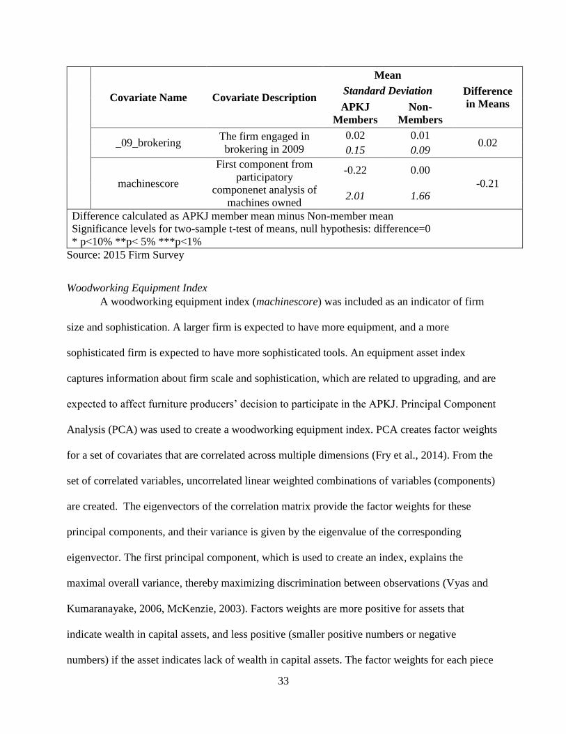
_09_brokering The firm engaged in

brokering in 2009

0.02 0.01 0.02

0.15 0.09

machinescore

First component from

participatory

componenet analysis of

machines owned

-0.22 0.00

-0.21 2.01 1.66

Difference calculated as APKJ member mean minus Non-member mean

Significance levels for two-sample t-test of means, null hypothesis: difference=0

* p<10% **p< 5% ***p<1%

Source: 2015 Firm Survey

Woodworking Equipment Index

A woodworking equipment index (machinescore) was included as an indicator of firm

size and sophistication. A larger firm is expected to have more equipment, and a more

sophisticated firm is expected to have more sophisticated tools. An equipment asset index

captures information about firm scale and sophistication, which are related to upgrading, and are

expected to affect furniture producers’ decision to participate in the APKJ. Principal Component

Analysis (PCA) was used to create a woodworking equipment index. PCA creates factor weights

for a set of covariates that are correlated across multiple dimensions (Fry et al., 2014). From the

set of correlated variables, uncorrelated linear weighted combinations of variables (components)

are created. The eigenvectors of the correlation matrix provide the factor weights for these

principal components, and their variance is given by the eigenvalue of the corresponding

eigenvector. The first principal component, which is used to create an index, explains the

maximal overall variance, thereby maximizing discrimination between observations (Vyas and

Kumaranayake, 2006, McKenzie, 2003). Factors weights are more positive for assets that

indicate wealth in capital assets, and less positive (smaller positive numbers or negative

numbers) if the asset indicates lack of wealth in capital assets. The factor weights for each piece

34

of woodworking equipment owned by a firm is summed to create woodworking equipment index

(machinescore), which is inserted directly into the model.

Twelve woodworking equipment variables were included in the PCA. Each is a count of

the number of pieces of equipment in a category. The categories are whipsaw, circle saw,

chainsaw, router, hand drill, planer, grinder, sander, spindle, jointer, a category that includes drill

presses and band saws, and another category for other woodworking equipment listed too few

times to be included as separate variables. Drill presses and band saws were grouped together

because of a lack of clarity in distinguishing between these two machines during survey

administration, as the names of these items are similar in Bahasa Indonesia. Furthermore, the

questionnaire contained an option for machine kit which included a few pieces of equipment.

When this option was selected, it was assumed that all items for this machine kit were owned,

but a distinction between drill press and band saw cannot be made. While these two pieces of

equipment serve different functions, they both enable precise work, and are similar in size and

price range. Since this is an integer rather than a binary variable, a firm that owns both a drill

press and a band saw will score higher on the machine index than a firm that owns only a drill

press, if all else is equal. Table 3 includes the descriptive statistics and factor weights for the

variables used to construct the machine index.

Table 3: Variables used in creation of woodworking equipment index

35

Variable Description Mean Std.

Dev.

Min Max Number

of cases

where

x>=1

Factor

Weight

Whipsaw 1.03 0.80 0 4 422 0.23

Circlesaw 0.29 0.47 0 3 163 0.37

Chainsaw 0.77 0.53 0 4 414 0.24

Router 0.01 0.12 0 1 8 -0.03

Hand drill 0.53 0.57 0 3 284 0.38

Planer 0.90 0.71 0 4 403 0.40

Grinder 0.72 0.69 0 3 331 0.31

Sander 0.61 0.56 0 4 332 0.41

Spindle 0.58 0.56 0 3 315 0.39

Jointer 0.05 0.23 0 2 29 0.15

Drill press and band saw 0.10 0.33 0 2 54 -0.06

Other 0.05 0.23 0 2 29 -0.07


Firm Scale

Several covariates provide information on the scale of the firm’s operations. An average

of the number of workers in the high, low and normal seasons during 2009 (recall data) was used

as a measure of firm scale. Twenty-six cases (8 members and 18 non-members) were missing

data on workers in 2009 due to enumerator error. In order to keep these cases in the analysis, the

number of workers in 2009 was regressed on the number of workers in 2015, and the predicted

values were used in place of missing 2009 information.

Total workshop area measured in meters (_09_totalm2_workshop_sum) also provided a

measure of firm scale. When two workshops were owned by the same firm, their area was

summed. Six cases (three members and three non-members) had missing data for workshop area.

36

For these cases, the predicted values from a linear regression of workshop area on total number

of workers in 2009 were used. Workshop area was left as zero if the firm did not own any

workshops in 2009. The number of total workshops owned in 2009 was also included as a

variable, _09_total_workshop, as was the total number of showrooms owned in 2009,

_09_total_showroom. Other business units related to the furniture industry were owned by some

firms, including showrooms, sawmills, kilns, and hardware stores. The variable _09_otherunits

measured the total number of furniture business units other than workshops and showrooms.

Business unit ownership is shown in table 4.

Table 4: Business unit ownership of APKJ members and control respondents before matching

Unit type Percent owning at least 1 of unit

type in 2009

APKJ

Members

APKJ

Non-Members

Workshop 93% 97%

Showroom 7% 9%

Sawmill 1% 0%

Large (Room-Sized) Oven 12% 4%

Logpark 0% 1%

Warehouse 2% 1%

Ironmongery (Hardware Shop) 1% 0%

Source: 2015 Jepara Firm Survey

Wood Used

Types of wood used for furniture production in 2009 recalled by the survey respondents

included teak, mahogany, mango, coconut, jackfruit, trembesi, sonokeling, and others. Teak and

mahogany were used most extensively. The percent of total wood used by the firm composed of

teak and mahogany (respectively) were used as variables in the model. Binary variables indicate

37

whether the teak/mahogany was sourced from Perum Perhutani, the offical state supplier of

timber (teak_tpk/mahoni_tpk).

Sales Channels

Three modules of the questionnaire used in 2015 gathered information about the way that

products were sold. These sections were: sales channels, buyers, and marketing. Information

from these three modules was combined to generate variables used in the model, as an

approximation of the sophistication of the firm’s sales strategy and buyers. Firms may have sold

products to other showrooms (_09_cbn_otsh); online, whether through their own website, a

group website, or through social media (_09_cbn_online); through a broker or trader

(_09_cbn_brok), to another workshop as part of a subcontracting arrangement (_09_cbn_sub); to

an exporter (_09_cbn_exp); directly to foreign and domestic buyers (_09_cbn_dir); or through

exhibitions (_09_cbn_exh). If a firm owns its own showroom, it is expected that products are

also sold through this channel. This effect is captured by including the variable

_09_total_showroom, which measures the number of showrooms owned by the firm. Since a

firm can sell through multiple channels, these variables are not mutually exclusive and do not

sum to one.

Furniture Types

Binary variables indicate what broad categories of furniture were produced by the

respondents in 2009. In order to not over-specify the model, basic furniture types were placed in

one general category (mebel_basic) that included vanity tables, beds, cabinets/wardrobes, chairs

and tables (both indoor and outdoor) and the catchall “other furniture types”. Separate, specific

binary variables were included for the production of wooden ornaments (im_ornamen_dekorasi),

calligraphy pieces (im_kerajinan_kaligrafi), room dividers (im_sketsel), and relief (im_relief),

the production of which suggest some level of specialization. A separate variable

38

(im_parts_komponen_mebel) was included for production of furniture components (such as chair

and table legs); this production suggests a lower level of upgrading than a firm that produces

whole furniture pieces. As noted in table 2, more APKJ members than sampled non-members

produced furniture pieces. When data on furniture produced in 2009 was missing, it was assumed

that furniture production in 2009 was the same as production in 2015. Four percent of sampled

non-members who were operating in 2015 were missing data for furniture types in 2009, and 3%

of APKJ members who were operating in 2015 were missing data for furniture types in 2009.

Sub-District (Kecamatan)

Kecamatan are the sub-district level of administration in Indonesia (Guggenheim et al.

2004). In the Kabupaten (district) of Jepara, where this survey was conducted, there are 15

Kecamatan. Binary variables were included in the model for all Kecamatan that contained at

least 5% of the sampling frame. Thus, the base group are cases located in Kecamatan with low

density of furniture businesses. Table 5 displays the percent of the sampling frame, treated units,

and non-treated units located in each Kecamatan. Those Kecamatan that were included as

variables in the model are highlighted in grey.

39

Table 5: Sub-district representation in current and past surveys

Total Sample APKJ Members Control Units 2010 frame

Name of

Kecamatan Count Percent Count Percent Count Percent Count Percent

Batealit 65 11% 14 12% 51 11% 186 14%

Jepara 45 8% 22 18% 23 5% 69 5%

Kedung 52 9% 10 8% 42 9% 166 13%

Mlonggo 101 18% 23 19% 78 17% 78 6%

Pakis Aji 60 11% 16 13% 44 10% 103 8%

Tahunan 195 34% 25 21% 170 38% 557 42%

Bangsri 1 0% 0 0% 1 0% 48 4%

Donorojo 4 1% 0 0% 4 1% 4 0%

Kalinyamatan 3 1% 1 1% 2 0% 7 1%

Keling 2 0% 0 0% 2 0% 1 0%

Kembang 10 2% 0 0% 10 2% 15 1%

Mayong 4 1% 0 0% 4 1% 14 1%

Nalumsari 0 0% 0 0% 0 0% 5 0%

Pecangaan 27 5% 8 7% 19 4% 57 4%

Welahan 2 0% 0 0% 2 0% 8 1%

Totals: 571 100% 119 100% 452 100% 1318 100%


Production Processes

Variables about production processes capture information about the firm’s level of

upgrading and its position of power within the value chain. Finishing furniture is a high value-

added activity. Respondents were asked to estimate the percent of production that was finished in

house, the percent that was contracted out to be finished, and the percent that was sold

unfinished. If a firm is contracting out work to another firm, it holds a position of relative power

over the firm that it has contracted to do the work. The final model included a binary variable,

which is equal to 1 if the firm sold finished pieces in 2009 (finishing_1). Including information

on finishing in this form was found to be best for balancing covariates. Another binary variable

was included which is equal to one when some percent of the construction and assembly was

contracted out to other workshops (contract_out_1). The questionnaire did not ask directly if

firms acted as brokers in 2009. However, it was presumed that a firm engaged in brokering in

40

2009 if it engaged in brokering in 2015, and reported contracting out in 2009, and the variable

_09_brokering was generated and used in estimating the propensity score.

Owner Characteristics

Since individual characteristics of the owner can influence the decision to participate in

an association, the owner’s age and education were also included as variables. When the owner’s

age in years was missing and the wife or child had responded, the owner’s age was estimated

using the sample median difference in age between husbands and wives or between a child and a

father (the median is equal to the rounded mean). The owner’s education was included as a

categorical variable. The questionnaire asked the respondents about their highest level of

education achieved. Degrees which require the same number of years of education were grouped

together. The categories are (i.) less than primary; (ii.) primary; (iii) SMP (middle school level);

(iv.) STM/SMK high school (technical track); (v.) SMA high school (academic track); (vi.)

tertiary education. A variable, _09_other_org_total, is a count of the other organizations of

which the owner is a member.

3.3.2 Outcome Variables

Testing each hypothesis requires different outcome variables. The first hypothesis, APKJ

members realize higher profits than non-members with similar attributes, required estimation of

firm profit based on information on costs and revenues collected during interviews. Respondents

could choose to record costs and revenues for a week, a month, or a year. Costs and revenues

were summed according to the time frame, and then scaled to year level to approximate firm

profit for the year as a whole. Costs that were accounted for in profit estimation are: wood

inputs, labor expenses, contracting-out costs, and other inputs and expenses such as

transportation, fuel, electricity, and oil/wax finishes.

41

Depreciation costs for woodworking equipment owned were not included in profit

calculation. Many observations are missing data on year acquired and/or price of purchase.

Furthermore, woodworking equipment used by small-scale producers is often makeshift in

nature, defying standard depreciation schedules. A woodworking equipment index similar to the

one described above, but using equipment owned in 2015 has a correlation coefficient with firm

profit of 0.076. While the correlation is significant at the 10% level, it is low enough that any

bias from excluding equipment depreciation costs can be expected to be minimal.

Revenues and expenses were scaled up from monthly/weekly to yearly using the

seasonality table in section six of the survey instrument, shown here in table 6. This table

categorizes each month of the year as part of low, normal, or high season, and includes an

estimate of production quantity for each month. These estimates were used to calculate average

monthly production during normal, high, and low seasons. The average for the seasonal level

that corresponds to that of the production and revenues table was then divided into the estimated

production quantity for each month. This created multipliers that could convert recorded costs

and revenues to costs and revenues for each month of the year according to seasonal variations.

The sample average for the appropriate multiplier (low to high, normal to low, etc.) was imputed

for cases that had seasonality information but were missing production averages (six cases).

Production was assumed to be constant for cases that lacked seasonality information and

monthly production estimates (five cases). Seasonality information that was specific to labor was

used to scale up labor costs. Respondents were asked the number of workers in low, normal and

high season, and multipliers were created from this information in a similar manner to what is

described above.

42

Table 6: Seasonality table from 2015 firm survey questionnaire

Aug Sep Oct Nov Dec Jan Feb Mar Apr May Jun Jul

Sea

son

Num

ber

of

Pro

duct

s

Sea

son

Num

ber

of

Pro

duct

s

Sea

son

Num

ber

of

Pro

duct

s

Sea

son

Num

ber

of

Pro

duct

s

Sea

son

Num

ber

of

Pro

duct

s

Sea

son

Num

ber

of

Pro

duct

s

Sea

son

Num

ber

of

Pro

duct

s

Sea

son

Num

ber

of

Pro

duct

s

Sea

son

Num

ber

of

Pro

duct

s

Sea

son

Num

ber

of

Pro

duct

s

Sea

son

Num

ber

of

Pro

duct

s

Sea

son

Num

ber

of

Pro

duct

s

Season code:

1=Low season

2=Normal season

3=High Season

Unit code:

1= pieces

2 = set

3 = container, 20ft

4= container, 40ft

5= container, 40HC

Source: 2015 Firm Questionnaire

This manner of accounting for firm profits is subject to limitations. The time frame of

inputs and outputs may not have always lined up properly, seasonality adjustments were

estimated, and there are variations in production and prices that were not captured by the survey

instrument. However, the information provided by the survey instrument delivers a rough

approximation of firm’s profits that can be used to assess the effect of APKJ membership on

profit levels. Prior to analysis, observations with very high or very low levels of profit were re-

examined. Fifteen observations were dropped because their profit estimations were

unrealistically high or low, or they were missing critical data. For some cases, the amount of

wood purchased did not appear to correspond with the amount of production in the given time

period. This is not surprising, as a firm may have purchased wood inputs that will be used for

production for more than one month, or had wood purchases left over from the previous month.

For two cases, the questionnaires specified that this was the case. In 25 other cases, examination

of wood input/furniture output ratios, along with consideration of the size of the piece that the

suggested by the price, indicated that wood inputs did not line up with furniture production for

43

that time period. For these twenty-seven observations, alternate wood quantities were used for

cost calculations based on an estimation of wood input per type of furniture output. Profit was

also calculated without the imputed levels of wood to compare. Treatment effects are also

estimated with the original wood costs to ascertain the impact of using alternate wood quantity

estimations.

The second hypothesis, that APKJ members have a higher probability than non-members

with similar attributes of increasing the sophistication of their marketing methods since 2009, is

evaluated by examining whether firms have picked up or dropped certain marketing and sales

channels between 2009 and 2015. These categories of marketing/sales channels were discussed

in section 3.3.1 as the 2009 values of these binary variables were used in calculating the

propensity score. Here, categorical variables comparing marketing and sales channel in 2015 and

2009 was used. These variables take on four values: 1 if the firm used the marketing method in

2009 and did not in 2015; 2 if the firm did not use the marketing method in either year, 3 if the

firm used the marketing method both years, and 4 if the firm used the marketing method in 2015

and not in 2009. Binary variables were also created to focus on adding or abandoning marketing

behaviors.

The third hypothesis, that APKJ members are more likely than non-members to have

upgraded their production activities since 2009, evaluates the difference in brokering and

finishing in 2009 and 2015. The variable indicating that the firm engaged in brokering in 2009,

discussed in the previous section, was compared with a variable indicating that the firm engaged

in brokering in 2015. Variables indicating whether the firm sold finished furniture in 2009 and

2015 were compared. Since it was not always clear whether the firm finished products in-house

or contracted out the finishing before selling the products, this outcome variable simply

44

compares whether furniture was finished upon leaving the firm, not whether the firm finishes

furniture. For brokering and finishing, categorical variables with categories analogous to those

described for marketing were generated. Binary versions of these variables were also created for

the analysis.

The fourth hypothesis, that APKJ members are more likely than non-members with

similar attributes to have good business management practices, was evaluated by comparing

2015 levels of good business practices by APKJ members and non-members. The practices

evaluated are record-keeping (records), having a registered business (registered) and being

SVLK certified (svlk).

This chapter described how propensity score matching is used to evaluate the outcome

variables of interest, explained the data collection process, and described the variables used in

the analysis. The next chapter discusses application of these methods, and results.

45

Chapter 4: Analysis and Results This chapter discusses implementation of the methods described in chapter three, and the

results obtained from application these methods. First, details of the empirical method are

discussed, including the commands used, decisions about caliper matching, and use of propensity

score matching with ordinal and categorical outcome variables. Next, the propensity score will

be evaluated based on common support and covariate balance criteria. Then, results from

propensity score matching are used to address each of the hypotheses listed in chapter one. For

the first hypothesis, profit differences between treated and control firms are evaluated as the

outcome variable. The second, third, and fourth hypotheses evaluate differences in sales

channels, marketing methods and production processes, as well as current business practices.

Following this, the effect of APKJ membership on businesses staying open, and the influence of

different factors on revenues and profit will be examined. Implications of the results reported in

this chapter are further addressed in chapter 5.

4.1: Implementing Empirical Methods

Propensity score matching was implemented in Stata® using the command “teffects

psmatch” (StataCorp, 2015). This command automatically calculates asymptotically unbiased

standard errors following the method put forward by Abadie and Imbens (2006). A disadvantage

of “teffects psmatch” is its inflexibility when restricting matches to a caliper. While the program

allows for a caliper to be specified, it exits with an error if a match for a unit is not found within

the specified caliper. Once the unmatched units are dropped, the user must run the command

again, and the propensity score will be re-calculated with the restricted sample. There is a lack of

clear guidance about whether the propensity score should be re-estimated after excluding units

for whom there are not matches within the caliper (Takeshima et al., 2016). Since the propensity

score that is estimated after dropping unmatched units will be different from the original

46

propensity score, distances between matches may be greater than in the original round.

Observations that were matched in the first iteration might not have matches within the caliper in

this second iteration. An older, user-written command, “psmatch2,” will drop the observations

without matches in their caliper from estimation of the treatment effect, and complete PSM

(Leuven and Sianesi, 2003b). However, “psmatch2” cannot calculate Abadie-Imbens standard

errors for propensity score matching (Leuven and Sianesi, 2003a).

When matching with a caliper, “teffects psmatch” was used with a caliper equal to 0.2

times the standard error of the logit model used to estimate the propensity. When matching to

one nearest neighbor with replacement (to calculate ATET) 13 unmatched APKJ members were

dropped from the dataset. Running “teffects psmatch” on this reduced dataset re-estimates the

propensity score. If a caliper equal to 0.2 standard deviations of the newly estimated propensity

score is required, 11 observations will not have matches within the caliper. The same is true if

the caliper is restricted to be less than 0.2 times the standard deviation of the original propensity

score. This pattern repeated itself for several iterations, resulting in an unjustifiably high loss of

treated units from the sample. To avoid this, “teffects psmatch” was implemented without a

caliper in the dataset from which the original 13 unmatched units were excluded. Since the

propensity score is re-estimated excluding the dropped units, this may lead to matches that are

different than in the original model (before dropping the units without matches within the

caliper).

In order to conduct detailed analysis with binary and categorical outcome variables,

datasets were created based on propensity score matches that allowed for the treated group to be

directly compared to the matched sample. The manipulated dataset that is based on the original

propensity score estimation consists of 84 APKJ members and the 84 nearest neighbor control

47

units. The differences in outcome means (proportions) of the binary outcome variables in the

manipulated dataset are equal to the treatment effects reported by the propensity score matching

commands in Stata.

Within the manipulated datasets, Fisher’s exact tests were used to examine whether there

is a significant relationship between the categorical outcome levels and APKJ membership. The

tabulated data allow for a clear comparison in the proportions of members and non-members

who added or abandoned different marketing/sales channels. Then, the binary versions of the

outcome variables were used to calculate risk ratios, and as the outcome variable for “teffects

psmatch.” Risk ratios are the cumulative incidence of the exposed units divided by the

cumulative incidence of the unexposed units. While statistical significance tests are not used with

risk ratios, if the confidence interval does not contain 1 then the risk ratio is considered

significant at the confidence level used by the confidence interval.

4.2: Checking Common Support and Covariate Balance Assumptions

The ATET is only defined within the region of common support. Visually examining the

graphed propensity score densities after matching intuitively displays the overlap. Figure 3

displays the propensity score density graphs for the treated and untreated groups when one

nearest neighbor (no caliper) is used to calculate the average treatment effect on the treated.

These graphs indicate sufficient common support to sustain propensity score matching; the

density graphs for treated and untreated units overlap substantially. However, the figure also

shows that the highest propensity scores belong to APKJ members exclusively. The region of

common support can be examined more precisely by comparing the highest and lowest

propensity scores in the treated and untreated groups. The lowest four propensity scores of the

untreated units all fall below 0.0001, while the lowest four propensity scores of the treated units

fall between 0.019 and 0.034. This disparity does not cause problems; when estimating the

48

ATET untreated units are matched to each treated unit, but treated units are not matched to each

untreated units. The highest four propensity scores of the untreated units are 0.739, 0.759, 0.775

and 0.919, considerably lower than the highest four propensity scores of APKJ members, 0.994,

0.996, 0.997 and 0.997. Furthermore, there may be spans within the range of common support

where there are not untreated units with similar propensity scores to treated units, leading to poor

matches.

Figure 3: Common support when matching to one nearest neighbor without a caliper


Common support and covariate balance were considered when choosing a matching

method. Caliper matching to one nearest neighbor was found to be the best option for improving

common support and covariate balance. Specifying a caliper requires the propensity scores of

matched units to be within a certain range. The caliper was specified as 0.05, or 0.2 times the

standard deviation from the logit model which calculated the propensity score. Thirteen treated

units did not have matches within the caliper, and were dropped from the estimation of the

treatment effect. The observations with the eight highest propensity scores were dropped, as well

as five observations with propensity scores between 0.82 and 0.85.

49

Percent standardized biases, t-tests of covariate means, and variance ratios were used to

evaluate balance after matching. T-tests for equality of means is conducted by the command

“pstest,” used after implementing propensity score matching with the command “psmatch2”

(Leuven and Sianesi, 2003b). The t-tests compare the covariate means of the treated and

untreated groups in the matched sample. Non-significant differences in covariates means suggest

relatively good covariate balance. Percent standardized bias, which standardizes the differences

in covariate means of two groups in order to be compared, is calculated using the formula below:

(1) SB =100∗(𝑥𝑡−𝑥𝑐)

√𝑆𝑡+2 𝑆𝑐

2

2

Where 𝑥𝑡 (𝑥𝑐) and 𝑠𝑡 (𝑠𝑐) are the mean and variance of the treated (control) groups. Low

standardized biases reflect good covariate balance. However, there is little formal guidance or

consensus on what constitutes an acceptable percent standardized bias. Normand et al. (2001)

implies that standardized biases lower than 10% are satisfactory, while Rosenbaum and Rubin

(1985) suggest that higher than 20% is concerning. Percent Standardized bias was obtained using

the command “teffects summarize” after propensity score matching with “teffects psmatch”

Variance ratios, the mean ratios of a covariates’ variance in the treated and untreated groups,

allow the researcher to evaluate the similarity of the distributions of covariates in for treated and

untreated groups after matching (Austin, 2009). The closer that variance ratios are to unity, the

more similar the distributions of covariates in treated and untreated groups. Variance ratios were

obtained through the “teffects summarize” command.

After matching to one nearest neighbor within a caliper, 20 out of 39 covariates has a

standardized bias equal to or higher than 10%, including 7 with standardized biases of 20% or

higher. The mean bias is 11.09% and the median bias is 9.74%. Two-sided t-tests found that 4

50

covariates were significantly different for matched treated and control groups. While some

covariates are not well-balanced after matching, this is not surprising given the large number of

covariates included.

Covariates are less balanced when matching to one nearest neighbor without a caliper,

when 5 covariate means are significantly different1, the mean bias is 15.44%, the median bias is

12.78%, and 27 covariates have a standardized bias of 10% or higher, 14 of which have

standardized biases of 20% or higher. When matching to five nearest neighbors specifying a

caliper is not feasible because it results in many treated units (39) being dropped from the

treatment effect estimation. Despite this, matching to five nearest neighbors without a caliper

produces slightly better balance between covariates than matching to one nearest neighbor within

a caliper. After matching to five nearest neighbors, only two covariates are significantly different

(at the 10% level), and seventeen covariates having a standardized bias of 10% or greater, seven

of which have a standardized bias of 20% or greater. Matching to one nearest neighbor within a

caliper is used primarily for the analysis, as it addresses both the concern of covariate balance

and of common support. Furthermore, matching to only one nearest neighbor is best for the

dataset manipulation performed for the evaluation of the outcome variables assessed for the

second, third and fourth hypotheses. A summary table comparing balance tests for three

matching methods is provided in Appendix B.

Matching to one nearest neighbor within a caliper is the most reliable method based on

covariate balance and common support. Conclusions about the impact of APKJ membership will

1 After matching to one nearest neighbor without a caliper, 3 covariate means are significantly different at the 10%

critical value and 2 covariate means are significantly different at the 5% critical value.

51

be drawn based on the treatment effects from this matching method. Results from matching to

one and five nearest neighbors without a caliper will also be presented as a point of comparison.

4.3: Hypotheses and Results

4.3.1: Hypothesis 1: APKJ members realize higher profits than non-members with similar

attributes

Benefits from any upgrading undertaken by a firm are predicted to be reflected as an

increase in profit. Since many factors influence profit, estimated profit serves as a

comprehensive but imprecise measure of the impact of the APKJ. Furthermore, profit is being

estimated based on information obtained through a survey, which may have incomplete data on

costs or revenues, or make imprecise assumptions about scaling up to a year.

There is a large range in estimated profit levels in both treated and untreated groups

before and after matching: figure 4 displays the kernel density graphs for estimated profit of

treated and untreated groups before matching, and figure 5 displays the kernel density graphs for

estimated profit of treated and untreated groups after matching. Summary statistics of firm profit

for APKJ members and non-members in the raw and matched datasets are provided in table 8. A

two-sample t-test of means shows that there is a significant difference in the profit levels of

members and non-members before matching on the propensity score. After matching, there is not

a significant difference in the profit levels of APKJ members and the counterfactual. The

difference for the matched dataset is equal to the treatment effect estimated by propensity score

matching. However, the sample standard deviations reported in table 7 do not account for the

propensity score having been estimated. Abadie-Imbens standard errors, which do account for

estimation of the propensity score, allow for reliable significance tests. Treatment effects from

propensity score matching, along with Abadie-Imbens standard errors, are reported in table 8.

52

Table 7: Descriptive statistics of estimated profit in treatment and control groups

Sample Treatment

Group Observations

Estimated Profit

Smallest Median Largest Mean Standard

Deviation

Difference

in Means

Raw (Unmatched)

APKJ

Members 98 -18,782 15,669 323,700 33,388 54,438

15,576** Non-

Members 385 -19,063 7,404 345,333 17,812 35,548

Matched to 1

Nearest Neighbor

(with caliper)

APKJ

Members 71 -14,083 13,547 323,700 31,967 54,646

2,572 Matched

Non-

members

71 -7,871 17,997 345,333 29,395 60,824

Significance levels for two-sample t-test of means, null hypothesis: difference=0

* p<10% **p< 5% ***p<1%


Figure 4: Kernel density of estimated profit for members and non-members before matching


Observations: 142

0

.000

01

.000

02

.000

03

.000

04

De

nsity

0 100000 200000 300000 400000Estimated Profit (Alt. Wood)

Members

Non-members

Estimated Profit

kernel = epanechnikov, bandwidth = 9.8e+03

Kernel density estimate

53

Figure 5: Kernel density of estimated profit after caliper matching to one nearest neighbor


Observations: 142

The treatment effects are positive but non-significant for matching to one nearest

neighbor within a caliper, indicating that APKJ membership does not have an effect on profits

(table 9). The treatment effect is also positive and non-significant after matching to five nearest

neighbors without a caliper. The difference is significant when matching to one nearest neighbor

without a caliper, but this does not provide sufficient evidence to conclude that there is a

significant difference in profit levels.

PSM was also applied to restricted samples. First, PSM was applied to a sample that

excluded firms whose 2015 operations included brokering. The effect was positive and

significant when matching to one nearest neighbor with and without a caliper (USD 14,014;

16,462). When the dataset excluded firms that engaged in brokering or owned a showroom in

2015, the treatment effects from all three matching methods were not significant. Next, extreme

profit levels were excluded. Examining the graphed kernel density of profit levels for the full

0

5.0

00e

-06

.000

01.0

00

01

5 .000

02.0

00

02

5D

ensity


Members

Non-members

Estimated Profit


Kernel density estimate

54

sample (see figure 6) suggested that $80,000 would serve as a sensible cutoff point, and the

dataset was restricted to observations with profit levels below that point. Caliper matching could

not be implemented, as there were perfect predictors of membership after dropping units without

matches within the caliper. The treatment effects calculated with this restricted sample were not

significant. Additionally, the treatment effect was estimated using a profit calculation that

included original costs for the 27 cases that had alternate wood quantity estimates. The treatment

effects in this case are smaller than when alternate wood quantities are used, and none of the

matching methods produces a significant effect.

Table 8: Average treatment effect on the treated for estimated firm profit (matching with

replacement)

Sample Restrictions/

Difference in

Outcome Variable

Measure

Number

of

Neighbors Caliper

Treatment

Effect, USD

Std. Err.

P-Value

Number of

Matched

Observations

None

1 Yes 2,572 11,397 0.82 142

1 10,828 5,770 0.06 168

5 3,498 6,189 0.57 168

Exclude cases that

broker in 2015

1 Yes 14,014 7,191 0.05 134

1 16,462 8,558 0.05 154

5 (5,655) 20,450 0.78 154

Exclude cases that

broker in or own

showrooms in 2015

1 Yes (26) 11,309 0.99 114

1 (6,024) 13,091 0.65 134

5 (8,201) 25,395 0.75 134

Exclude Profit above

USD 80,000

Propensity score cannot be estimated (perfect predictors)

1 (5,230) 5,497 0.34 148

5 888 4,674 0.85 148

Use original wood

costs in profit

calculation (not

alternate estimates)

1 Yes 734 11,785 0.95 142

1 7,486 6,727 0.27 168

5 661 6,586 0.92 168


55

Figure 6: Kernel density of estimated profit of full sample


Observations: 483

Firm revenue was also examined as an outcome variable. There is expected to be less

error in the revenues estimate than in the estimate of profit. Reporting sales information is more

straightforward than reporting cost information, and misalignment of costs and revenues does not

affect revenues. However, revenues are more reflective of the scale of a firm’s operations than of

livelihood effects, as high cost of inputs may erode most or all firm revenue. Still, firm revenue

is an informative outcome variable that indicates a firm’s level of success. Figure 7 compares

revenues for members and non-members after matching to one nearest neighbor with a caliper.

Like estimated profit, there is a very large range in estimated revenue levels.

0

.000

01

.000

02

.000

03

De

nsity



Kernel density estimate of estimated profit of full sample

56

Figure 7: Kernel density of estimated revenues after caliper matching to one nearest neighbor


Observations: 142

The treatment effects for firm revenues, reported in table 9, reflect those for profit. As

with the profit outcome variable, the treatment effects are positive and significant when matching

to one nearest neighbor without a caliper when there are no dataset restrictions, and when

matching to one nearest with or without a caliper after excluding firms that broker. Other

matching methods yield non-significant results. These results further suggest but do not confirm

the possibility of a livelihood impact of membership.

0

5.0

00e

-06 .000

01.0

00

01

5 .000

02.0

00

02

5D

ensity

0 200000 400000 600000Estimated revenues in USD

Members

Non-members


Comparison of members and nonmembers

Kernel density of estimated revenues

57

Table 9:Average treatment effect on the treated for estimated firm profit (matching with

replacement)

Sample

Restrictions/

Difference in

Outcome Variable

Measure

Number of

Neighbors Caliper

Treatment

Effect,

USD

Std.

Err. z

P-

Value

Number of

Matched

Observations

None

1 Yes -1,126 19,113 -0.06 0.95 142

1 17,849 6,961 2.56 0.01 168

5 8,863 9,276 0.96 0.34 168

Exclude cases that

broker in 2015

1 Yes 22,488 4,236 5 0.00 134

1 34,045 11,700 3 0.00 154

5 -6,586 36,258 0 0.86 154

Exclude cases that

broker in or own

showrooms in 2015

1 Yes 8,394 18,946 0 0.66 114

1 -12,193 22,507 -1 0.59 134

5 -13,538 44,270 0 0.76 134


4.3.2: Hypothesis 2: APKJ members have a higher probability than non-members of

increasing the sophistication of their marketing methods between 2009 and 2015

To evaluate this hypothesis, categorical variables were created to compare

marketing/sales channels in 2009 and 2015. This categorical variable took on four values: 1 if the

firm utilized a sales channel in 2009 that it did not utilize in 2015; 2 if the firm did not a sales

channel in 2009 and 2015; 3 if the firm utilized a sales channel in 2009 and 2015, and 4 if the

firm utilized a sales channel in 2015 that it did not in 2009. Either adding or abandoning a sales

channel can be seen as upgrading, depending on the sophistication and power of the channel in

question. The categorical variables compare changes in selling through other showrooms

(chg_cbn_otsh), selling directly to buyers (diff_cbn_dir), selling through a broker

(diff_cbn_brok), selling through exhibitions (diff_cbn_exh), selling through an exporter

(diff_cbn_exp), being subcontracted (diff_cbn_sub), and selling online (diff_cbn_online).

Additional binary variables were created to focus on firms that added or abandoned a

marketing/sales channel between 2009 and 2015. The variables focusing on adding a

58

marketing/sales channel (pc_diff_cbn_[marketing/sales channel]) equal 1 if the firm added that

sales channel between 2009 and 2015, and equal 0 otherwise. The variables focusing on

abandoning a marketing/sales channel (nc_diff_cbn_[marketing/sales channel]) equal 1 if the

firm abandoned that sales channel between 2009 and 2015, and equal 0 otherwise. Variables on

marketing/sales channels were excluded from calculation of the propensity score used to match

units for the analysis of these outcome variables. Caliper matching with one nearest neighbor

was used.

There is a significant relationship between the addition of exhibition attendance and

APKJ membership (table 9). Twelve percent more APKJ members than the matched

counterfactual adopted selling through exhibitions. The addition of exhibition attendance as a

sales and marketing channel represents increased sophistication of marketing. The significant

effect of membership on attendance validates the efforts of the Jepara FVC Project’s moving up

scenario to support exhibition attendance. While the treatment effect for abandoning selling

through exhibitions is also positive and significant, this may be because APKJ members

confused exhibitions attended in 2010 with 2009 exhibitions.

Table 10: Tabulated data, treatment effects, and risk ratios for changes in the practice of

marketing through exhibitions (2009-2015)

Outcome variable Measure Values

Changes in practice of marketing through

exhibitions, 2009-2015 (chg_cbn_exh)

% Non-

members

%

Members

Abandoned 1 0% 3%

Neither year 2 95% 82%

Both years 3 5% 4%

Added 4 0% 12%

P-value from Fishers Exact Test 0.00

Matched Observations (total) 152

59

Binary variable indicating the firm added

marketing through exhibitions

between 2009 and 2015: pc_diff_cbn_exh

(1 if added ; 0 otherwise)

risk ratio2 N/A3

P-value

Treatment Effect 0.12

AI Standard Error 0.04

P-value 0.00

Binary variable indicating the firm

abandoned marketing through exhibitions

between 2009 and 2015: nc_diff_cbn_exh

(1 if abandoned ; 0 otherwise)

risk ratio N/A

p-value



P-value 0.03

After matching to one nearest neighbor within a caliper; ATET

Source: 2015 Survey data, which included recall questions on operations in 2009

The relationship between APKJ membership and change in whether a firm sells directly

to buyers is significant at the 1% level (table 10). Thirteen percent of the matched sample of

APKJ members began selling directly to buyers between 2009 and 2015, contrasting with only

4% of the counterfactual group. However, more producers in the APKJ than in the matched

control group also stopped selling directly to buyers in the same time span. The treatment effects

for both adding and abandoning selling directly to buyers are positive and significant. Since

producers who engage in market-based interaction directly with buyers have bargaining power

and are able to negotiate prices and product specifications, these results show that APKJ

members are more likely to either improve their bargaining power by beginning to sell directly to

buyers, or to decrease their bargaining power by abandoning selling directly to buyers.

2 Risk ratios are calculated as the cumulative incidence of the exposed units divided by the cumulative incidence of

the unexposed units. While statistical significance tests are not used with risk ratios, if the confidence interval does

not contain 1 then the risk ratio is considered significant at the significance level used by the confidence interval. 3 Risk ratios cannot be calculated when any value is zero

60


directly to buyers (2009-2015)

There is not a significant relationship between APKJ membership and adoption of online

marketing (table 11), although a goal of The Jepara FVC Project was fostering the use of online

marketing and sales channels by discussing online marketing in training sessions and launching a

marketing website (www.javamebel.com) for members to use.

Table 12: Tabulated data, treatment effects, and risk ratios for changes in use of practice of

online marketing (2009-2015)

Outcome Variable Measure Values

Changes in practice of marketing

online, 2009-2015

(chg_cbn_online)

% Non-

members

%

Members

Abandon 1 1% 1%


Both years 3 7% 1%

Add 4 49% 45%




Changes in practice of selling directly

to buyers, 2009-2015 (chg_cbn_dir)

% Non-

members

%

Members

Abandoned 1 1% 9%


Both years 3 21% 30%

Added 4 4% 13%



Binary variable indicating addition of

selling directly to buyers between

2009 to 2015: pc_diff_cbn_dir (1 if

added ; 0 otherwise)

risk ratio 3.33

P-value <0.10



P-value 0.01

Binary variable indicating

abandoning selling directly to buyers

2009 - 2015: nc_diff_cbn_dir (1 if

abandoned ; 0 otherwise)

risk ratio 7.00

P-value <0.10



P-value 0.01



61


marketing online between 2009 to

2015: pc_diff_cbn_online (1 if added ;

0 otherwise)

risk ratio 0.91

P-value ≥0.10

Treatment Effect

AI Standard Error

-0.04

0.07

P-value 0.57

Binary variable indicating abandoning

selling through another showroom

from 2009 to 2015:

nc_diff_cbn_online (1 if abandoned ;

0 otherwise)

risk ratio 1.00

P-value ≥0.10

Treatment Effect

AI Standard Error

0.00

0.02

P-value 1.00



The relationship between APKJ membership and change in selling through an exporter is

significant at 1% (table 12). APKJ membership has a significant, positive effect on adding and

abandoning selling through an exporter. Selling furniture through an exporter suggests that a firm

is capable of adhering to international standards, but involves directed networks in which

exporters, not producers, have bargaining power. Therefore it is unclear which change would be

considered upgrading.

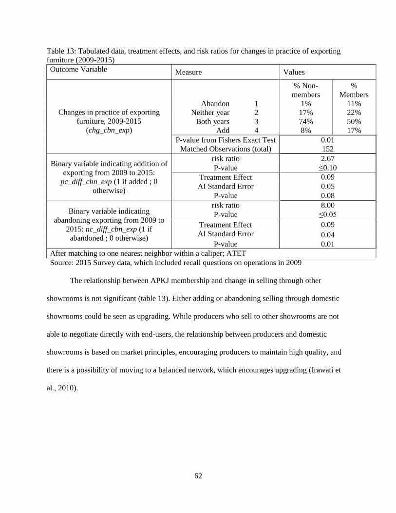
62

Table 13: Tabulated data, treatment effects, and risk ratios for changes in practice of exporting

furniture (2009-2015)


Changes in practice of exporting

furniture, 2009-2015

(chg_cbn_exp)

% Non-

members

%

Members

Abandon 1 1% 11%



Add 4 8% 17%




exporting from 2009 to 2015:

pc_diff_cbn_exp (1 if added ; 0

otherwise)

risk ratio 2.67

P-value ≤0.10

Treatment Effect

AI Standard Error

0.09

0.05

P-value 0.08


abandoning exporting from 2009 to

2015: nc_diff_cbn_exp (1 if


risk ratio 8.00

P-value ≤0.05

Treatment Effect

AI Standard Error

0.09

0.04

P-value 0.01



The relationship between APKJ membership and change in selling through other

showrooms is not significant (table 13). Either adding or abandoning selling through domestic

showrooms could be seen as upgrading. While producers who sell to other showrooms are not

able to negotiate directly with end-users, the relationship between producers and domestic

showrooms is based on market principles, encouraging producers to maintain high quality, and

there is a possibility of moving to a balanced network, which encourages upgrading (Irawati et

al., 2010).

63


through other showrooms (2009-2015)

Outcome Variables Measure Values

Changes in practice of selling

through other showrooms, 2009-2015

(chg_cbn_otsh)

% Non-

members

%

Members

Abandon 1 7% 9%



Add 4 8% 5%




selling through another showroom

from 2009 to 2015: pc_diff_cbn_otsh

(1 if added ; 0 otherwise)

risk ratio 0.67

P-value ≥0.10

Treatment Effect

AI Standard Error

-0.03

0.04

P-value 0.56


abandoning selling through another

showroom from 2009 to 2015:

nc_diff_cbn_otsh (1 if added ; 0

otherwise)

risk ratio 1.40

P-value ≥0.10

Treatment Effect


0.03

P-value 0.39



Membership in the APKJ does not have a significant effect on change in selling to

brokers (table 14), or on being subcontracted by other firms (table 15). Selling to a broker and

being subcontracted both represent positions of very low bargaining power, where the buyer

defines the product and the price. A larger percent of APKJ members than matched non-

members started being subcontracted between 2009 and 2015, and fewer members abandoned

being subcontracted than in the counterfactual group.

64


through (to) brokers (2009-2015)

Outcome Variables Measure Values

Changes in practice of selling

through (to) brokers, 2009-2015

(chg_cbn_brok)

% Non-

members

%

Members

Abandon 1 4% 7%


Both years 3 5% 20%

Add 4 41% 30%



Binary variable indicating addition

of selling through (to) brokers from

2009 to 2015: pc_diff_cbn_brok (1 if


risk ratio 0.77

P-value ≥0.10

Treatment Effect -0.11


P-value 0.25


abandoning selling through (to)

brokers from 2009 to 2015:

nc_diff_cbn_brok (1 if added ; 0

otherwise)

risk ratio 1.67

P-value ≥0.10



P-value 0.45



Table 16: Tabulated data, treatment effects, and risk ratios for changes in practice of being

subcontracted (2009-2015)


Changes in practice of being

subcontracted, 2009-2015

(chg_cbn_sub)

% Non-

members

%

Members

Abandon 1 33% 32%


Both years 3 8% 9%

Add 4 16% 20%




being subcontracted between 2009 to

2015: pc_diff_cbn_sub (1 if added ; 0

otherwise)

risk ratio 1.25

P-value ≥0.10



P-value 0.58

65

Binary variable indicating abandoning

being subcontracted between 2009 to

2015: nc_diff_cbn_sub (1 if

abandoned; 0 otherwise)

risk ratio 0.96

P-value ≥0.10



P-value 0.92



These findings demonstrate varying levels of success of the Jepara FVC Project’s efforts

to improve small scale producers’ marketing practices and bargaining power. Producers are more

likely to abandon selling through brokers and begin selling directly to buyers and at exhibitions

if they are members of the APKJ than if they did not join the association. Yet at the same,

members are more likely to abandon selling directly to buyers and are no more likely to abandon

being subcontracted or add online marketing than if they had not joined. It appears that the

Jepara FVC met with the most success when the APKJ facilitated a specific behavior such as

exhibition attendance.

4.3.3: Hypothesis 3: APKJ members are more likely than non-members to have upgraded

their production activities since 2009

There is a significant relationship between APKJ membership and changing from not

brokering in 2009 to brokering in 2015 (table 16). Brokering is a position with substantial

bargaining power, which allows brokers to receive a larger portion of the final price than is

received by someone who functions only as a wood carver. Brokering requires business acumen

that APKJ training workshops sought to impart.

66

Table 17: Tabulated data, treatment effects, and risk ratios for changes in brokering status 2009-

2015


Changes in brokering status, 2009-

2015 (categorical variable

chg_brokering)

% Non-

members

%

Members


Both years 3 1% 2%

Add 4 0% 6%



Changes in brokering status, 2009-

2015 (binary variable

diff_brokering)



P-value 0.02



More APKJ members than matched non-members stopped selling finished furniture

between 2009 and 2015, and more matched non-members than non-members began selling

finished furniture in the same time period (table 17). Like brokering, finishing is an ‘upgraded’

production activity. It allows firms to attain a larger portion of the final price than they would

through carving, and requires skills and knowledge that were taught in APKJ training

workshops. However, these workshops have not had a significant effect on adding production of

finished products.

Table 18: Tabulated data, treatment effects, and risk ratios for changes in selling finished

products 2009-2015


Changes in practice of finishing

products, 2009-2015

(chg_finished)

% Non-

members % Members

Abandon 1 1% 8%



Add 4 20% 11%



67


addition of selling finished

products between 2009 to 2015:

pc_diff_finsihed (1 if added ; 0

otherwise)

risk ratio 0.53

P-value ≤0.10



P-value 0.01


abandoning selling finished

products between 2009 to 2015:

nc_diff_finished (1 if added ; 0

otherwise)

risk ratio 7

P-value ≤0.10



P-value 0.01



These results present a mixed picture of the influence of the APKJ on upgrading

production activities. More APKJ members than the counterfactual began brokering since the

formation of the APKJ, indicating a shift to a position with bargaining power that takes a large

portion of the final product’s value. On the other hand, significantly more APKJ members than

non-members stopped selling finished products. These results suggest that the Jepara FVC

Project was more successful in facilitating functional upgrading that involves marketing and

bargaining power (brokering) rather than production processes (finishing).

4.3.4: Hypothesis 4: APKJ members are more likely than non-members to have good

business management practices

Training workshops conducted as part of the Jepara Furniture Value Chain Project

encouraged application of good business management practices such as record-keeping and

officially registering the business. The Jepara FVC project also encouraged obtaining SVLK

certification by providing training workshops on the process, and facilitating the formation of

groups to obtain group certification. The results for business registration and SVLK certification

show that APKJ members are more likely than non-members to have good business management

practices, though members are no more likely than non-members to keep business records.

Ten percent of APKJ members in the matched sample have SVLK certification, as

opposed to 6% of matched non-members (table 18). The treatment effect is significant at the 1%

68

level. Empowering small-scale producers to obtain SVLK certification was a key focus of the

Jepara Furniture Value Chain Project. While only a modest number of APKJ members have

obtained certification, the treatment effect shows that the influence of membership on obtaining

certification is positive and significant.

Table 19: Tabulated data, treatment effects, and risk ratios for SVLK certification


SVLK certification in

2015 (svlk): 1 certified; 0

if not certified

% Non-

members

%

Members

Not Certified 0 94% 90%

Certified 1 6% 10%



risk ratio 1.75

P-value ≥0.10



P-value 0.00


Source: 2015 Survey data

There is not a significant relationship between APKJ membership and keeping records or

having a registered business (tables 19 and 20) 4. However, this is a cross-sectional comparison

rather than a differenced outcome variable.

4 Propensity score matching with the outcome variable records, unlike the other upgrading outcome variables, was

conducted without a caliper. When a caliper was used with the records outcome variable, the covariate

_09_brokering predicted APKJ membership perfectly, so the propensity score could not be estimated.

69

Table 20: Tabulated data, treatment effects, and risk ratios for record-keeping


Record-keeping in 2015

(records): 1 if firms

keeps records; 0 if does

not keep records

% Non-

members

%

Members

Records 0 63% 71%

No Records 1 37% 29%



risk ratio 0.79

P-value ≥0.10



P-value 0.69



Table 21: Tabulated data, treatment effects, and risk ratios for business registration


Registered business in

2015 (registered): 1 if

firm is registered; 0 if not

registered

% Non-

members

%

Members

Not Registered 0 77% 64%

Registered 1 23% 36%



risk ratio 1.53

P-value ≥0.10



P-value 0.16


Source: 2015 Survey data

4.3.5: Revenue Predictors and Staying Open versus Shutting Down

The third objective of this study is to measure the impact of specific upgrading behaviors

on revenues and profits. To do so, business practices and characteristics were used as

independent variables in an ordinary least square regression, with profit or revenues as the

dependent variable. In order to take the natural log of estimated profit, it was first adjusted so

that all values were positive. When the natural log of adjusted estimated profit was used as the

dependent variable, the only independent variable with a significant effect was the average

70

number of workers; the addition of one worker generates a 2% increase in profit, all else held

constant.

When the natural log of yearly revenues, rather than profit, was used as the outcome

variable, more independent variables had a statistically significant effect. The output from this

model is shown in table 21. This model showed that an additional worker increased revenues by

4.5%, and an additional square meter increased revenues by 0.1%. The interaction term for these

two variables was not significant. Despite project implementers’ high hopes for the effect of

SVLK certification, this model did not show certification to have a significant effect on

revenues. Brokering has a dramatic impact on revenues; firms that broker are shown to have

60.3% higher profit than firms that do not broker. Surprisingly, selling directly to buyers had a

significant negative effect, decreasing revenues by 14.5%. Online marketing, conversely, has a

positive effect of 23.5%. Selling at exhibitions increases revenues by 44.8. Selling to exporters

also increases revenues by 19.6%.

Table 22: Ordinary least square estimates for predictors of firm revenues

Variables Variable Description Coefficient

Standard

Error

_15_worker_avg Average number of workers 0.04*** 0.01

_15_totalm2

_workshop_sum

Total meters squared of

workshop space 0.00*** 0.00

worker_m2

Interaction term for workers and

workshop space 0.00 0.00

brokering

Equals 1 if the firm engaged in

brokering 0.60*** 0.21

svlk_or_skema

Equals 1 if the firm had SVLK

certification -0.14 0.21

_15_finished

Equals 1 if the firm sold finished

products 0.03 0.12

_15_total_showroom

The number of showrooms

owned by the firm 0.09 0.14

71

Variables Variable Description Coefficient

Standard

Error

_15_cbn_otsh

Equals 1 if the firm sold furniture

to/through a showroom with a

different owner 0.00 0.11

_15_cbn_dir


directly to buyers -0.14* 0.09

_15_cbn_online


online 0.24** 0.09

_15_cbn_brok


through a broker or trader 0.11 0.09

_15_cbn_exh


through exhibitions 0.45** 0.19

_15_cbn_exp


to exporters 0.20** 0.10

_15_cbn_sub

Equals 1 if the firm was

subcontracted -0.03 0.11

Constant 19.14 0.11

F(14, 468)=11.80

Prob > F=0

R-squared=0.26

Adjusted R-

squared=0.24


While surveying, it was found that some firms had closed down, including seventeen

APKJ members. Fourteen APKJ members had shut down their businesses as a result of business-

related problems, while three had shut down because of death or illness. With the intent of

determining whether APKJ membership helped businesses to stay afloat, data on operations in

2009 were collected from firms that had closed down. As table 23 shows, APKJ members are

0.47 times as likely as non-members to shut down. This analysis was conducted without

complete data, as many non-members that were originally selected from the sampling frame to

72

be respondents were not interviewed because they could not be found or had moved away. It is

likely that many of these potential cases did shut down.

Table 23: Tabulated data, treatment effects, and risk ratios for businesses closing


Closed

(The firm closed

between 2009 and

2015 for business

reasons)

% Non-

members

%

Members

Open 0 78% 90%

Closed 1 22% 10%



risk ratio 0.47

P-value <0.05



P-value 0.02

4.4: Qualitative Survey Responses

The survey conducted in summer 2015 asked respondents about the benefits of APKJ

membership. Training, improved access to credit, improved market access, increased access to

raw materials, and help with means of production were provided as potential answers for the

enumerators to mark. A blank space was also provided in the questionnaire for any other opinion

of members. Aggregated responses are provided in table 23. Ninety members (67%) listed

training as a benefit. Eight (7%) listed improved credit access, 15 (13%) listed improved market

access, 12 (10%) listed increased access to raw materials, and 10 (8%) listed help with means of

production.

Several members added a comment about the APKJ. Forty-two members said that they

had gained insight, knowledge, market access, experience or opportunities, and 11 emphasized

the opportunity to build relationships that the APKJ had created. Additionally, two members

reported borrowing woodworking equipment from the APKJ as a benefit of membership.

73

However, fifteen members added a comment indicating that they had not experienced any benefit

from the association. Two of these members had joined late, in 2013, missing the training

sessions that had been provided through CIFOR.

Table 24: Member-identified benefits of the APKJ

Benefits of Membership

Number of APKJ

Members

Sugges

ted

resp

onse

s

Training 90

Credit 8

Market 15

Raw Materials 12

Production 10

Fre

e re

sponse

No benefits 15

Knowledge 34

Improved production quality 2

Gained Friends/Colleagues 12

Experience 8

marketing/market access/exhibition/opportunities 4

Borrowed woodworking equipment 2

4.5: Conclusion and Limitations

These findings indicate that there is a limited, positive impact of APKJ membership.

Profit and revenue treatment effects provide some evidence of a positive effect of membership,

and other outcome variables indicate that membership does have some influence on members’

marketing, production, and business practices. However, the conclusion of each hypothesis is

unclear, as there is some evidence supporting each conclusion and some evidence against it.

Through the APKJ, the Jepara FVC project influenced members to upgrade by participating in

exhibitions, selling directly to buyers, beginning to sell finished products, obtaining SVLK

certification, and moving towards becoming brokers. However, APKJ members are also more

likely to abandon selling directly to buyers and stop selling finished products, and no more likely

to being marketing online or stop selling through brokers. The implications of these results are

74

further discussed in the next chapter. This discussion will aid in understanding what this

evaluation means for future projects.

The treatment effects for upgrading outcomes indicate that APKJ members changed more

(for better and for worse) than the control units matched to them. These bimodal outcomes for

members may be indicative of the APKJ attracting two different types of furniture producers:

one type whose business is not doing well that joins the APKJ in hopes of improvement, and

another type who is particularly motivated and views the APKJ as an opportunity to be

developed in order to improve their business. It appears that the APKJ did not succeed in

improving the firms of the first type of members, but that the members of the second type were

able to leverage the opportunities and resources of the APKJ to improve their businesses.

Several factors limited the study. First, the study uses data on what a respondent could

recall about their operations six years prior to survey administration. The recall data are included

in estimation of the propensity score, which is relied upon for the results reported in this chapter,

as well as for a baseline in the calculation of outcome variables. Additionally, the estimation of

profit is based on survey responses. These responses do not include costs such as rent or a

mortgage, depreciation expenses or debt expenses. Production and input time spans are not

uniform so information for costs and revenues may not correspond, and assumptions about

seasonality and consistency were used when scaling up costs and revenues to a year.

Furthermore, the likelihood of getting significant results with the profit outcome variable is

limited by the small sample size for treated units and the large variance in estimated profit.

Propensity score matching was implemented in order to minimize selection bias. However,

membership and outcome variables may have been influenced by unobservable characteristics

that were not account for when estimating the propensity score.

75

Chapter 5: Discussion The focus of this study was to determine the impact of membership in the APKJ. This

was achieved by using propensity score matching to quantify the livelihood impact of the project

by comparing firm profits of APKJ members against a counterfactual (sub-objective 1), and

determine the extent of the uptake of upgrading behaviors promoted by the four upgrading

scenarios of the Jepara FVC project (sub-objective 2). Two additional models, using profit and

revenues as outcome variables, achieved the third objective of measuring the impact of specific

upgrading behaviors on revenues and profits. The purpose in pursuing these objectives was to

evaluate the Jepara Furniture Value Chain Project, the objectives of which were “(i). to enhance

the structure and function of the furniture industry for the benefit of small-scale furniture

producers; (ii). to improve marketing by small-scale furniture producers and their industry

associations, and (iii). to monitor changes regarding the effects and early acceptance of

innovations from objectives 1 and 2 and revise and/or reinforce project strategies accordingly”

(Purnomo et al., 2013).

The first objective of the Jepara FVC Project requires the influence of the project to

affect the entire furniture industry of Jepara. The policy roadmap works towards the achievement

of this objective, but its efficacy cannot yet be evaluated. An assessment report being drafted by

CIFOR about the Jepara FVC notes the important role of CIFOR in passing the legislation, and is

optimistic about the capacity of the policy to improve the structure and function of the Jepara

furniture value chain. Portions of local budgets have been allocated to implement this policy.

CIFOR should follow up on the implementation of this policy by examining how the allocated

budget is spent, and determining how many producers benefit from implementation of the policy.

Evaluating the APKJ in 2015, before the policy was fully implemented, provides an

opportunity to examine the impact of changes that the policy hoped to achieve in the value chain

76

as a whole. While the APKJ did not alter the structure and function of the entire furniture value

chain for the benefit of small-scale producers, participation in the APKJ improved bargaining

power of some members. A significantly higher percentage of APKJ members than matched

control units (the counterfactual) abandoned selling to a broker, which affords little power for

negotiation in product specification or pricing. Additionally, a significantly higher percentage of

APKJ members than non-members began brokering, a position with substantial market power

that claims a large portion of the product’s final value. More APKJ members than non-members

also obtained SVLK certification, providing more opportunities to sell to buyers in Europe.

Additionally, there is some evidence that membership in the APKJ membership improves

livelihoods, suggesting that members are better able to function within the current structure of

the value chain.

The second objective, as far as it relates to APKJ members, has been specifically

addressed in this study. The proportions of members and non-members that adopted online

marketing were similar. More APKJ members than non-members began marketing through

exhibitions, which affords them the opportunity to interact directly with buyers and develop their

own brand. More APKJ members than non-members also began selling directly to buyers from

2009 to 2015. However, more APKJ members than non-members also stopped selling directly to

buyers in the same time span.

The third objective relates to the research method employed by the project, and the

manner in which policy recommendations were synthesized. The knowledge generated by the

project allowed researchers to pinpoint inefficiencies in the value chain. However, translating

research findings into tangible outcomes is not always possible. Addressing many of the

challenges identified by the value chain analysis, such as timber scarcity, lack of access to credit,

77

low bargaining power, and international competition are beyond the scope of a single project or

policy. Furthermore, allocating fewer resources to defining challenges, and more resources to

providing outreach to participants, will likely lead to better outcomes.

The project’s design relied on several assumptions which should be further examined.

Upgrading was seen as a means to improve all producers’ livelihoods. While some upgrading

activities such as obtaining SVLK certification and improving product quality add value to

current production, the project also promoted moving up in the value chain. Shifting to or

incorporating a higher stage in the value chain, such as finishing furniture or brokering, has

potential to allow an individual to realize a larger portion of the final value of a product.

However, uniformly encouraging producers to move up to higher stages of the value chain

ignores the economic principal of comparative advantage, and disregards the interdependence of

value chain actors. Since actors are needed at all levels of the value chain, unvaryingly

encouraging actors to move up in the value chain does not represent a sustainable solution to the

challenges faced by the industry. Furthermore, the anticipated impacts of the project relied on

expectations that APKJ members would share knowledge, and that the APKJ would grow and

become independent were not realized. The project directly engaged only with APKJ members

and other attendees of training sessions, a very small portion of the furniture producers in Jepara:

APKJ membership totals 125, while there are over 11,000 business units in Jepara’s furniture

industry. Project designers must be wary of basing expected impacts on assumptions such as

independent growth of the APKJ.

Conclusions can be made from this project that can guide the design of future projects to

increase impact. First, project designers should carefully consider investment in knowledge-

generating activities, such as conducting value-chain analysis, over outreach activities, such as

training sessions. Second, assumptions about the way in which improvements are achieved (such

78

as upgrading) must be carefully evaluated to determine if they hold in the context of the project.

Third, evaluation of expectations for knowledge diffusion should ensure that the expectations are

realistic and viable.

79

References ABADIE, A. & IMBENS, G. W. 2006. Large sample properties of matching estimators for

average treatment effects. econometrica, 74, 235-267.

ABADIE, A. & IMBENS, G. W. 2008. On the failure of the bootstrap for matching estimators.

Econometrica, 76, 1537-1557.

ABADIE, A. & IMBENS, G. W. 2009. Matching on the estimated propensity score. National

Bureau of Economic Research.

ACHDIAWAN, R. & PURNOMO, H. 2010. Livelihood strategies of small-scale furniture

producers in Jepara (Central Java) in facing tight market competition.

ALDRICH, J. H. & NELSON, F. D. 1995. THE LINEAR PROBABILITY MODEL. Linear

Probability, Logit, and Probit Models. SAGE Publications, Inc, Thousand Oaks, CA,

SAGE Publications, Inc.

AUSTIN, P. C. 2009. Balance diagnostics for comparing the distribution of baseline covariates

between treatment groups in propensity‐score matched samples. Statistics in medicine,

28, 3083-3107.

CALIENDO, M. & KOPEINIG, S. 2008. SOME PRACTICAL GUIDANCE FOR THE

IMPLEMENTATION OF PROPENSITY SCORE MATCHING. Journal of Economic

Surveys, 22, 31-72.

DEHEJIA, R. H. & WAHBA, S. 2002. Propensity Score-Matching Methods for

Nonexperimental Causal Studies. The Review of Economics and Statistics, 84, 151-161.

EFFENDI, R. & PARLINAH, N. 2009. Leading firms, power relations and existing rules. Bogor

Agricultural University.

FISHMAN, A. & OBIDZINSKI, K. 2013. Verified Legal? Ramifications of the EU Timber

Regulation and Indonesia’s Voluntary Partnership Agreement for the Legality of

Indonesian Timber. CIFOR

FRY, K., FIRESTONE, R. & CHAKRABORTY, N. M. 2014. Measuring Equity with Nationally

Representative Wealth Quintiles. Washington, DC: PSI.

GARRIDO, M. M., KELLEY, A. S., PARIS, J., ROZA, K., MEIER, D. E., MORRISON, R. S.

& ALDRIDGE, M. D. 2014. Methods for Constructing and Assessing Propensity Scores.

Health Services Research, 49, 1701-1720.

GEREFFI, G., HUMPHREY, J. & STURGEON, T. 2005. The governance of global value

chains. Review of international political economy, 12, 78-104.

HECKMAN, J. J., ICHIMURA, H. & TODD, P. E. 1997. Matching as an Econometric

Evaluation Estimator: Evidence from Evaluating a Job Training Programme. The Review

of Economic Studies, 64, 605-654.

HENRICH, J. 2001. Cultural Transmission and the Diffusion of Innovations: Adoption

Dynamics Indicate That Biased Cultural Transmission Is the Predominate Force in

Behavioral Change. American Anthropologist, 103, 992-1013.

HERR, M. L. & MUZIRA, T. J. 2009. Value chain development for decent work: a guide for

development practitioners, government and private sector initiatives.

HUMPHREY, J. & SCHMITZ, H. 2002. How does insertion in global value chains affect

upgrading in industrial clusters? Regional studies, 36, 1017-1027.

ICHINO, A., MEALLI, F. & NANNICINI, T. 2008. From Temporary Help Jobs to Permanent

Employment: What Can We Learn from Matching Estimators and Their Sensitivity?

Journal of Applied Econometrics, 23, 305-327.

IRAWATI, R. H., MELATI & PURNOMO, H. 2010. Analysis of value chain governance:

scenarios to develop small - scale furniture producers.

80

KHANDKER, S. R., KOOLWAL, G. B. & SAMAD, H. A. 2010. Handbook on impact

evaluation: quantitative methods and practices, World Bank Publications.

LEUVEN, E. & SIANESI, B. 2003a. help for psmatch2 [Online]. Available:

http://repec.org/bocode/p/psmatch2.html [Accessed June 12 2016].

LEUVEN, E. & SIANESI, B. 2003b. PSMATCH2: Stata module to perform full Mahalanobis

and propensity score matching, common support graphing, and covariate imbalance

testing. 4.0.11 22oct2014 ed.

LOEBIS, L. & SCHMITZ, H. 2005. Java furniture makers: Globalisation winners or losers?

Development in Practice, 15, 514-521.

MCCORMICK, D. & SCHMITZ, H. 2001. Manual for value chain research on homeworkers in

the garment industry. mimeo, Institute of Development Studies, Nairobi and Sussex.

MCKENZIE, D. J. 2003. Measuring inequality with asset indicators. Journal of Population

Economics, 18, 229-260.

MELATI, PURNOMO, H. & SHANTIKO, B. 2013. Making research work for small-scale

furniture makers: Action research in the Jepara furniture industry, Indonesia, Bogor,

Indonesia, Center for International Forestry Research (CIFOR).

NORMAND, S.-L. T., LANDRUM, M. B., GUADAGNOLI, E., AYANIAN, J. Z., RYAN, T. J.,

CLEARY, P. D. & MCNEIL, B. J. 2001. Validating recommendations for coronary

angiography following acute myocardial infarction in the elderly: A matched analysis

using propensity scores. Journal of Clinical Epidemiology, 54, 387-398.

OZANNE, L. K. & VLOSKY, R. P. 1997. Willingness to pay for environmentally certified

wood products: A consumer perspective. Forest Products Journal, 47, 39-48.

PRESTVIK, A. 2009. Small-scale furniture producers in Jepara. Survey report. Bogor,

Indonesia: CIFOR.

PURNOMO, H., ACHDIAWAN, R., MELATI, IRAWATI, R. H., SULTHON, SHANTIKO, B.

& WARDELL, A. 2014. Value-chain dynamics: strengthening the institution of small-

scale furniture producers to improve their value addition.

PURNOMO, H., ACHDIAWAN, R., SHANTIKO, B., AMIN, S. M., IRAWATI, R. H.,

MELATI & WARDELL, A. 2016. Multi-stakeholder processes for strengthening policy

affecting small and medium-scale forestry enterprises.

PURNOMO, H., IRAWATI, R. H., ACHDIAWAN, R., SULTHON, SHANTIKO, B. &

MELATI 2013a. Action research approach to strengthening small-scale furniture

producers in Indonesia through policy development.

PURNOMO, H., SHANTIKO, B., IRAWATI, R. H., ACHDIAWAN, R., PUNTODEWO, A.,

(CIFOR), M. A., PARLINAH, N., (FORDA), R. E., YOVI, E. Y., NURROCHMAT, D.

R., (IPB), B., AMIN, S. M., ARYA, M., ARY, L. & ZAINUDIN, A. 2013b. Final report

for: Mahogany and teak furniture: action research to improve value chain efficiency and

enhance livelihoods. Australian Centre for International Forestry Research (ACIAR).

RODA, J.-M., CADÈNE, P., GUIZOL, P., SANTOSO, L. & UZAIR FAUZAN, A. 2007. Atlas

of wooden furniture industry in Jepara, Indonesia, Fauzan. Montpellier, France: French

Agricultural Research Centre for International Development (CIRAD) and Bogor,

Indonesia: Center for International Forestry Research (CIFOR).

RODRIGUEZ, D. G. P., REJESUS, R. M. & ARAGON, C. T. 2007. Impact of an Agricultural

Development Program for Poor Coconut Producers in the Philippines: An Approach

Using Panel Data and Propensity Score Matching Techniques. Journal of Agricultural

and Resource Economics, 32, 534-557.

RODRÍGUEZ, G. 2007. Lecture Notes on Generalized Linear Models.

http://repec.org/bocode/p/psmatch2.html

81

ROSENBAUM, P. R. & RUBIN, D. B. 1983. The central role of the propensity score in

observational studies for causal effects. Biometrika, 70, 41-55.

ROSENBAUM, P. R. & RUBIN, D. B. 1985. Constructing a control group using multivariate

matched sampling methods that incorporate the propensity score. The American

Statistician, 39, 33-38.

RUBEN, R. & ZUNIGA, G. 2010. How standards compete: comparative impact of coffee

certification schemes in Northern Nicaragua. Supply Chain Management: An

International Journal, 16, 98-109.

SMITH, J. A. & TODD, P. E. 2005. Does matching overcome LaLonde's critique of

nonexperimental estimators? Journal of Econometrics, 125, 305-353.

STATACORP. 2015. teffects psmatch — Propensity-score matching [Online]. College Station,

TX: Stata Press. Available: http://www.stata.com/manuals13/teteffectspsmatch.pdf

[Accessed May 2 2016].

TAKESHIMA, H., ADHIKARI, R. P. & KUMAR, A. 2016. Is access to tractor service a

binding constraint for Nepali Terai farmers?, Intl Food Policy Res Inst.

TRIENEKENS, J. H. 2011. Agricultural value chains in developing countries a framework for

analysis. International Food and Agribusiness Management Review, 14.

VAN GEENHUIZEN, M., INDARTI, N. & SOETANTO, D. P. 2010. Knowledge acquisition

and innovation: potentials for upgrading of very small and small firms in furniture

manufacturing in Indonesia. International Journal of Foresight and Innovation Policy, 6,

207-224.

VEISTEN, K. 2007. Willingness to pay for eco-labelled wood furniture: Choice-based conjoint

analysis versus open-ended contingent valuation. Journal of Forest Economics, 13, 29-

48.

VERHOFSTADT, E. & MAERTENS, M. 2014. Smallholder cooperatives and agricultural

performance in Rwanda: do organizational differences matter? Agricultural Economics,

n/a-n/a.

VLOSKY, R. P., OZANNE, L. K. & FONTENOT, R. J. 1999. A conceptual model of US

consumer willingness‐to‐pay for environmentally certified wood products. Journal of

Consumer Marketing, 16, 122-140.

VYAS, S. & KUMARANAYAKE, L. 2006. Constructing socio-economic status indices: how to

use principal components analysis. Health Policy and Planning, 21, 459-468.

WOLLNI, M. & ZELLER, M. 2007. Do farmers benefit from participating in specialty markets

and cooperatives? The case of coffee marketing in Costa Rica1. Agricultural Economics,

37, 243-248.

WOOLDRIDGE, J. M. 2009. Introductory Econometrics: A Modern Approach, Delhi, India,

Cengage.

YOVI, E. Y., BAHRUNI & NURROCHMAT, D. R. 2009. Sources of Timber and Constraints to

the Timber Acquisition of Jepara`s Small-Scale Furniture Industries.

http://www.stata.com/manuals13/teteffectspsmatch.pdf

82

Appendix A: Survey Questionnaire

Survey for Impact Study of the Jepara Furniture Value Chain

Project

I. Control Information

I. Identification

1. Sample ID: _______________________

2. Name of workshop/Furniture business (if none leave blank) __________________________

3. Address: Street_______________________________ No.____ RT_____ RW_______

Dusun ____________ Desa___________________ Kecamatan______________

4. Respondent name____________________________________________________

5. Owner name ___________________________________________________________

6. GPS reference of workshop location (UTM format):

a. slide__ __ grid __ __ ordinal__ __

b. Lattitude_______________________ Longitude______________________ (Titik GPS)

7. APKJ member? Yes _______ No______

8. APKJ champion? Yes_______ No______

II. Owner Characteristics

A. Respondent

1. Age _________years

2. Gender: Male Female

3. Highest level of education achieved by respondent: ____

1. Did not graduate SD/ Did not attend formal school 6. SMA or equivalent

2. SD or equivalent 7. Akademi/

Diploma

3. SMP or equivalent 8. S1

4. STM/ SMK 9. S2 or higher

5. SMK Ukir 4. Is the respondent the workshop owner? Yes_____ No____ If yes, proceed to section IV. If not,

please answer the following questions

5. Role of respondent: Manager____ Worker/ craftsman______ Other_______

6. Do you receive salary/ wages or profit/income from the business’s operations?

7. If so, what is the daily rate ? Rp________________________/ hari

8. Age of workshop owner _________years

9. Gender of workshop owner : Male Female

10. Highest level of education achieved by workshop owner:

A B C

Task Name Date

DD/MM/Year

Status OK? If

not, comment

1 Interview

2 Check Questionnaire

3 Enter data

83

1. Did not graduate SD/ Did not attend formal school 6. SMA or equivalent

2. SD or equivalent 7. Akademi/ Diploma

3. SMP or equivalent 8. S1

4. STM/ SMK 9. S2 or higher

5. SMK Ukir

84

Business Unit

Table IV.1: Current Business units (all units owned since 2009)

A B C D E F G H I J K

Type of business

units

1=Workshop

2=Showroom

3=Sawmill

4=Large Drying

Oven

5=Logpark

6=Warehouse

7=Ironmoger

Business Unit

Name

Year

Opene

d

Check if

still

open

How many

years has

the

business

been closed

If closed,

why did it

close?

The number

of similar

business

units in the

same RT

(administrat

ive unit)

The distance

to the center of

the Kecamatan

Located

with the

owner’s

home?

Size of

business

unit in

square

meters Kilom

eters

Minut

es

walki

ng

1 Km M2

2 Km M2

3 Km M2

4 Km M2

5 Km M2

6 Km M2

7 Km M2

8 Km M2

9 Km M2

1

0

Km M2

85

A. Other current characteristics of business

1. Is it a family-owned business? Yes________ No_____

2. What percent (%) of the family’s income comes from furniture production ________%

3. Does the business have a record of revenues and expenditures? Yes ____ No_____

4. Number of workers during:

High Season _____ Low Season______ Normal or average __________

5. Is the business formally registered? Yes_____ No______

6. If yes, what type of registration?

i. IRT (Industri Rumah Tangga/Domestic Industry), village or RT license

ii. UD (Usaha Dagang/trading business)

iii. CV

iv. PT

v. Other, write-in ___________

Table IV.2: Certification

A B C D E F

Certification Does the business unit have

any certification?

Mark if yes

Has the business unit

had this certification

before?

Mark if yes

Is this part of a

group

certification?

How many

members are in

the group?

How many members

of the group are

APKJ members?

1 SVLK

2 Skema SVLK

2 FSC

3 LEI

4 SGS

5 Other

86

Table IV.3 : Industry/Trade Organizations

What industry/trade organizations is the business unit owner a member of?

A B C D E F G

Organization

1=APKJ |

2=ASMINDO

3=Komunitas Pengrajin

Mebel Nasional (KPMN)

4= AMKRI

5 = KADIN

6=other (please specify)

Year Joined Still a

member?

If left the organization,

why did the owner leave?

How active in the organization?

1=Very active, attended all

meetings/events

2=Somewhat active, attending

meetings/events sometimes

3=Not too active – attended

several meetings/events

4=Not active – never attend

meetings/events

What kind of support have

you received from the

organization?

1=Training

2=Increase access to credit

3=Increase market access

4= Improved access to raw

materials

5=Assistance with the tools

for production

What are the main

advantages of being a

member ?

1

2

3

4

5

6

7

87

V. State of the furniture business in 2009 (Refer to the 2009 elections for recall)

A. This business unit had been established by 2009 (If so, please check, if not go to section VI) ______

1. Did you have a record of expenditures and revenues for your business in 2009? Yes_____ No_______

2. If records were kept in 2009, please record revenues from that year ________________

3. If records were kept in 2009, please record wood costs from that year_______________

4. Number of employees

High season (max) _____ Low season (Min)______ Normal or average________

Table V.1: Furniture type produced in 2009

Please check if produced in 2009

A

Furniture type Check if yes

1 Outdoor chair

2 outdoor table

3 Outdoor table and chair set

4 Chair indoor

5 Indoor table

6 Indoor chair and table set

7 Vanity table

8 Patio umbrella

9 Wardrobe/cabinet

10 Bed

11 Carved crafts and calligraphy

12 Simple crafts

13 Ornaments, decoration

14 Room divider

88

15 Relief

16 TV table

17 Parts/furniture parts

18 Other (please specify)

89

Table V.2: Sales Channel

Please write the percent of sales that occurs through each channel

A B

Jalur Check if Yes Percent

1 Firm Website %

2 Group Website %

3 Firm’s own Showroom %

4 Other showroom %

5 Subcontracted by another firm %

6 Facebook/other social media %

7 Direct sales to buyers at exhibitions %

8 Direct sales to buyers through personal

communication

%

9 Direct sales to other types of buyers %

10 Sold to exporter %

11 Sold to traders/brokers %

12 Sold directly to ther buyers/other buyers from abroad %

90

Table V.3: Marketing

Marketing methods used in 2009. Check if used the marketing method in 2009 and rank by importance to

the firm.

A B

Marketing method Check if Yes Rank (1=The most important)

1 Not doing anything

2 The buyer comes to the workshop/warehouse

(buyer orders)

3 Newspaper

4 Make brochure

5 Look for buyers in a place with a lot of people

(tourist attractions, restaurants, etc.)

6 Own marketing website

7 www.javamebel.com

8 Group marketing website

9 Participate in exhibitions

10 Facebook/Other social media

Table V.4: Buyers: Please fill in the following information about buyers in 2009

A B C

Check if

yes

Where/from

where?

(Location

Code)

Where does the

buyer sell it?

(Location code)

1 Were there buyers from other workshops in 2009?

2 Buyers from other showrooms in 2009?

3 Was the business selling to an exporter in 2009?

4 Did you sell to a broker/trader in 2009? (Y/N)

5 Are the products sold directly to the consumer? (Y/N)

Location Code

1=Jepara 2=Somewhere else in Indonesia 3=Europe 4=China/ Hong Kong 5=India 6= Somewhere else 7=Not

known


91

Table V. 5: Production process coordination 2009

A B C D E

What percentage of the

construction of furniture

is contracted out to other

artisans? ( 0 if none)

What percentage (%)

of product assembly

furniture craftsmen

contracted out to other

artisans? (0 if never)

Columns C, D, and E should total 100%

What percent of

products is sold

unfinished?

What is the

percent of

product of

products that are

finished in the

workshop?

What percent of the

products are contracted

out to other artisans for

finishing?

% % % % %

92

Table.V.6 Wood used in 2009

No Type of Wood

Ch

eck

if

yes

Per

cen

t (

%)

C. Sourcce of Wood Please

provide the percent of each timber

source that wood inputs were

composed of in 2009

D. Timber source (location) In 2009, where did the

business unit source wood from? List percent from each

location

Per

huta

ni/

TP

K

Com

munit

y t

eak

fore

sts

Pri

vat

e

Est

ates

Dis

edia

kan

pem

bel

i

Import

Jepar

a

Wes

t Ja

va

Eas

t Ja

va

Cen

tral

Java

Sula

wes

i

Import

Oth

er

Not

know

n

1 Teah

2 Mahogany

3 Mango

4 Coconut

5 Durian

6 Trembesi

7 Sonokeling

8 Old teak (from

dismantled

structures)

9 Oak

10 Other, specify ___

93

VI. Current Marketing

Table VI.1: Sales Channels

tolong tunjukan berapa prosentase dari penjulan di workshop/ brak dan showroom/ toko mebel setiap jalurnya

sampai saat ini

A B

Jalur/sumber Check if Yes

Percent Sold Through

Channel

1 Own Marketing Website %

2 www.javamebel.com (APKJ website) %

3 Group Marketing Website %

4 Own Showroom %

5 Sell to other showroom %

6 Receives orders from a large workshop %

7 Facebook/other social media %

8 Sell directly to buyers at exhibitions %

9 Sell to buyers that are known personally %

10 Sell directly to buyers (other) %

11 Sell to exporter %

12 Sell to broker %

13 Sell directly to buyers %

94

Table VI.2: Current Marketing

Rank marketing according to importance

A B

Marketing Method Check if Yes Rank

1 Not doing anything

2 The buyer comes to the workshop/warehouse

(buyer orders)

3 Newspaper

4 Make brochure

5 Look for buyers in a place with a lot of people

(tourist attractions, restaurants, etc.)

6 Own marketing website

7 www.javamebel.com

8 Group marketing website

9 Participate in exhibitions

10 Facebook/Other social media

Question VI.1: How is the selling price determined?

1. Decide for self

2. Decided by buyer

3. Negotiated with buyer

4. Other, specify


95

Table V1.3: Buyers: Please fill in the following information about buyers in 2009

A B C

Check if

yes

Where/from

where?

(Location

Code)

Where does the

buyer sell it?

(Location code)

1 Were there buyers from other workshops in 2009?

2 Buyers from other showrooms in 2009?

3 Was the business selling to an exporter in 2009?

4 Did you sell to a broker/trader in 2009? (Y/N)

5 Are the products sold directly to the consumer? (Y/N)

Location Code

1=Jepara 2=Somewhere else in Indonesia 3=Europe 4=China/ Hong Kong 5=India 6= Somewhere else 7=Not

known

Table VI.4: Exhibits attended in last year

Record the exhibitions were attended by representatives of the firm in the last year (Juli2014-Juni 2015)

A B C D E

Exhibition: Jepara Semarang Jakarta Somewhere else in

Indonesia

Another country

1 Total exhibition attended

2 State where:

96

VII. Production and sales

Table VII.1 Production during the year July 2014-June 2015

Time period: _______Week ________Month ______Year Season: ______Low ______Normal _____High

A B C D E F G H I J K L M

Productio

n Unit

Which

production processes

are

performed by your

business?

1=Making furniture

components

2=Merakit 3=Finishing

4=

Everything 5=Compone

nt and

assembly (unfinished)

6=Assembl

y and finishing

7 =

Components &

finishing 8=

brokering/

trading/ marketing

Check furniture types Wood

(see code)

If part of

the constructi

on is

contracted to other

artisans,

at what cost? Rp

If part

of the assembl

y is

contracted to

other

artisans, at what

cost?

Rp

Is the product

finished when sold?

(Y/T)

If

finishing is

contracte

d to other artisans,

at what

cost? Rp

Total

production in time

period

Pric

e per

unit

(Rp/ Unit

)

Tota

l (Rp)

1= pieces

2= set

3=Furniture

componen

ts 4=

Container

20ft 5=

Container

40ft 6=

Container

40HC 7= Truck

8 =

Pickup i. O

utd

oo

r C

hai

r

ii. O

utd

oo

r T

able

iii.

In

doo

r C

hai

r

iv. In

do

or

Tab

le

v.

Pat

io U

mb

rell

a

vi.

War

dro

be/

Cab

inet

vii

. B

ed

vii

i. C

arved

cra

fts

& c

alli

gra

ph

y

ix. D

eco

rati

on

/orn

amen

t

x.

Van

ity

tab

le

xi.

Roo

m d

ivid

er

xii

. R

elie

f

xii

i. F

urn

itu

re p

arts

xiv

. O

ther

fu

rnit

ure

xv. o

ther

(sp

ecif

y)

Typ

e o

f w

ood

Wo

od

Sou

rce

Wo

od

Sou

rce

(lo

cati

on

)

1

2

3

4

5

6

7

97

Table VII.2 Product seasonality: Write the number of products manufactured each month and whether the month was low, high, or normal season

August September October November December January February March April May June July Unit

Sea

son

Nu

mb

er o

f P

rod

uct

s

Sea

son

Nu

mb

er o

f P

rod

uct

s

Sea

son

Nu

mb

er o

f P

rod

uct

s

Sea

son

Nu

mb

er o

f P

rod

uct

s

Sea

son

Nu

mb

er o

f P

rod

uct

s

Sea

son

Nu

mb

er o

f P

rod

uct

s

Sea

son

Nu

mb

er o

f P

rod

uct

s

Sea

son

Nu

mb

er o

f P

rod

uct

s

Sea

son

Nu

mb

er o

f P

rod

uct

s

Sea

son

Nu

mb

er o

f P

rod

uct

s

Sea

son

Nu

mb

er o

f P

rod

uct

s

Sea

son

Nu

mb

er o

f P

rod

uct

s

1= piece

2 = set

3 = container

20ft

4= container

40ft

5= container

40HC

Season:

1= Low Season

2= Normal/ average

3= High season

A. Type of wood

1. Teak 6. Sonokoling

2. Durian 7. Mango

3. Old teak (disassembled) 8. Oak wood

4. Trembesi 9. Coconut

5. Mahogany 10. Other, specify

B. Wood source

1. Perhutani/TPK

2. Community forestry

3. Private estates

4. From buyer

5. Import

C. Wood source (location)

1.Jepara 6. East Java

2.Central Java 7. Import

3. Other

4. West Java

5. Sulawesi

98

Other revenues July 2014-June 2015

1. Revenues workshop Rp _________________________

2. Revenues showroom/ Toko Mebel Rp _________________________

3. Oms Revenues et logpark/ TPK Rp _________________________

4. Revenues Oven/ Pengeringan Rp _________________________

5. Revenues penggergajian Rp _________________________

VIII. Inputs

Table VIII.1Wood purchase time frame week____, month______ or year____) A B C D E F G H I J K

Type

of

wood

(see

code)

Source of

raw

materials?

Source of

raw

materials

(location)?

Are the

raw

materials

SVLK

certified?

Quantity Unit

1= m3

2= truck

3= pick

up

4 =bilah

5=volume

6 = Other

Price

per

unit

Bentuk kayu

1=plank/

kayu

gergajian

2=kayu bulat

3=borongan

4= lainnya,

sebutkan

Total

spent

(Rp)

If purchased

in the form

of

log/timber,

what are

sawmill

costs? What

is an

estimate of

these costs

if they saw

in-house Rp

Mark if

sawmill

in-

house

Cost of

drying

kiln if

dried

before

assembly

(if own

kiln what

is an

estimate

of the

cost)?

Check if

firm has

own

drying

kiln

1

2

3

99

4

5

A. Type of wood

1. Teak 6. Sonokoling

2. Durian 7. Mango

3. Old teak (disassembled) 8. Oak wood

4. Trembesi 9. Coconut

5. Mahogany 10. Other, specify

B. Wood source

6. Perhutani/TPK

7. Community forestry

8. Private estates

9. From buyer

10. Import

C. Wood source (location)

1.Jepara 6. East Java

2.Central Java 7. Import

3. Other

4. West Java

5. Sulawesi

100

See table VIII.1

Table VIII.2 Workers

Number

of

Workers

Number of

female workers

Number of

male workers

Amount paid to

female workers

Number of

workers with

SMK

Carving

degree

Number of workers

with SMK/SMT or

SMA (high school

level) degrees

During May 2015

During the year

Table VIII.3: Other inputs in May

A B C D E

Jumlah yang

digunakan

berdasarkan dalam

bulan Mei 2015

Dicatat pada

bulan Mei

2015

Unit Harga per

unit (Rp/

Unit)

Total (Rp)

1 Fuel

2 Diesel Fuel

3 Electricity

4 Transportation (for transporting wood purchased, finished products,

product showroom, etc.)

5 Paint/finish/melamine

6 Other

Total cost of product sold in the firm’s showroom that are not produced in the firm’s own workshop Rp_____________________

101

IX. Loans and Credit

X. Capital Assets

Table X.1: Machines currently owned (and those owned in 2009 not currently owned)

A B C D E

Machines category Year of acquisition/purchase Price (Rp) Still owned?

Check if yes

If not owned currently,

how was the machine

Table IX. Loans taken out over the last 6 years

A B C D E F G H

Source of

loan

Year Purpose Interest Interest

1=Monthly

2=Yearly

The amount

borrowed (Rp)

Total paid (Rp) Amount for

each

installment

(Rp)

1

2

3

4

5

6

7

8

9

10

11

12

13

14

15

(A) Loan source

1. Bank 7. Loan from Buyer

2. APKJ cooperation 8. Private moneylenders

3. Other cooperation 9. Family/friends

4. Credit Card 10. Pawnshop

5. Business micro-credit 11. Other source

6. Input loan from suppliers

(C) Purpose of loan

1. Family/private

2. Capital for business

3. Transportation

4. Machines

5. Building

6. Other

102

discarded of (sold,

thrown out, given away)

1

2

3

4

5

6

7

8

9

10

11

12

13

14

15

16

17

18

19

20

103

Table X.2: Transportation assets owned since 2009

A B C D E

1 Transportation category

(see code)

Year of

acquisition/purchase

Price (Rp) Still owned?

Check if yes

If not owned currently, how was the

mode of transport discarded of (sold,

thrown out, given away)

2

3

4

5

6

7

8

9

10

(A) Code

1. Pick up

2. Truck

3. Motor bike

4. Car

5. Other

Kategori mesin: (1) Gergaji Selendang; (2) Amplas mesin/ (3) Gerinda; (4) Bor; (5) Spindel; (6) Bengkok + kikir; (7) circle saw/ gergaji

piringan; (8) Mesin 1 paket (bobok, pasah, bor, cerke, gergaji bengkok); (9) Profil; (10) Kompresor; (11); gergaji tangan; (12) Planner; (13)

lainnya

105

XI. Participation in Training Sessions

Table XI.1: Training Sessions

A B C

1 Pelatihan Please mark

if a

representative

of the

business

participated

Did you

apply

what you

learned

in this

training

session?

Mark if

yes

What, if anything, did you gain

from this training session?

2 Quality control: (a) quality standards, (b)

wood-drying techniques, (c) making

simple drying kilns

(8 April 2010)

3 Financial management: (a) accessing and

managing bank loans, (b) calculating

costs, (c) managing financial matters

(9 April 2010)

4 Chain of custody certification

(27–29 July 2010)

5 Exhibition management (28 September

2010)

6 Management and motivation training for

small-scale furniture producers

(3–4 October 2010)

7 Furniture finishing and

entrepreneurialism

(11–12 May 2011)

8 Training on design development

106

(18–22 July 2011)

9 Training on exhibition preparation

(October 2011)

10 Entrepreneurialism for women

(15–16 November 2011)

11 Marketing assistance for SMEs in Jepara

and financial management and funding

(26 November, 17 December 2011)

12 Carving and design training for women

(28 February, 1 March 2012)

13 Wood preservation training

(8–9 March 2012)

14 Image editing

(18 April 2012)

15 SVLK training (19–20 February 2012,

27–29 April, May 2012)

16 Training on production: Tools (JIG) for

spindle moulder and circular saw

(30 June–1 July 2012)

17 Improving performance of the furniture

and timber industry in Central Java

(19 July 2012)

18 Training in kilns and drying

(24 September 2012)

19 Furniture design training

(17–29 October 2012)

107

Table XI.2: Other training sessions

Describe any training sessions attended in the last 6 years

A B C D

Date Topic Sponsor Location

1

2

3

4

5

6

7

8

9

10

108

Appendix B: Balance Tests T-tests for equality of means is conducted by the command “pstest,” which is used after implementing propensity score matching with

the command “psmatch2” (Leuven and Sianesi, 2003b). The t-tests compare the covariate means in the matched sample.

Percent standardized bias, which standardizes the differences in covariate means of two groups in order to be compared, is calculated

using the formula below:

(1) SB =100∗(𝑥𝑡−𝑥𝑐)

√𝑆𝑡+2 𝑆𝑐

2

2

Where 𝑥𝑡 (𝑥𝑐) and 𝑠𝑡 (𝑠𝑐) are the mean and variance of the treated (control) groups. Low standardized biases reflect good covariate

balance. However, there is little formal guidance or consensus on what constitutes an acceptable percent standardized bias. Normand

et al. (2001) implies that standardized biases lower than 10% are satisfactory, while Rosenbaum and Rubin (1985) suggest that higher

than 20% is concerning. Percent Standardized bias was obtained using the command “teffects summarize” after propensity score

matching with “teffects psmatch.”

Variance ratios, the mean ratios of a covariates’ variance in the treated and untreated groups, allow the researcher to evaluate the

similarity of the distributions of covariates in for treated and untreated groups after matching (Austin, 2009). The closer that variance

ratios are to unity, the more similar the distributions of covariates in treated and untreated groups. Variance ratios were obtained

through the “teffects summarize” command

Table B1: Comparison of balance measures of three matching methods

Nearest Neighbor Matching

1 Nearest Neighbor 5 Nearest Neighbors

Caliper No Caliper No Caliper

Covariate Name p>|t|

%

Bias

Variance

Ratio p>|t|

Percent

Bias

Variance

Ratio p>|t|

Percent

Bias

Variance

Ratio

_09_oth_org_total 1.00 0% 1.00 1.00 0% 1.00 0.41 13% 1.95

machinescore 0.26 -19% 1.14 0.16 -23% 1.17 0.99 0% 1.27

_09_brokering 0.16 24% . 0.16 19% . 0.16 22% .

finishing_1 0.06 33% 1.71 0.00 43% 2.13 0.56 9% 1.10

contract_out_1 0.04 34% . 0.25 15% 2.41 0.59 -8% 0.75

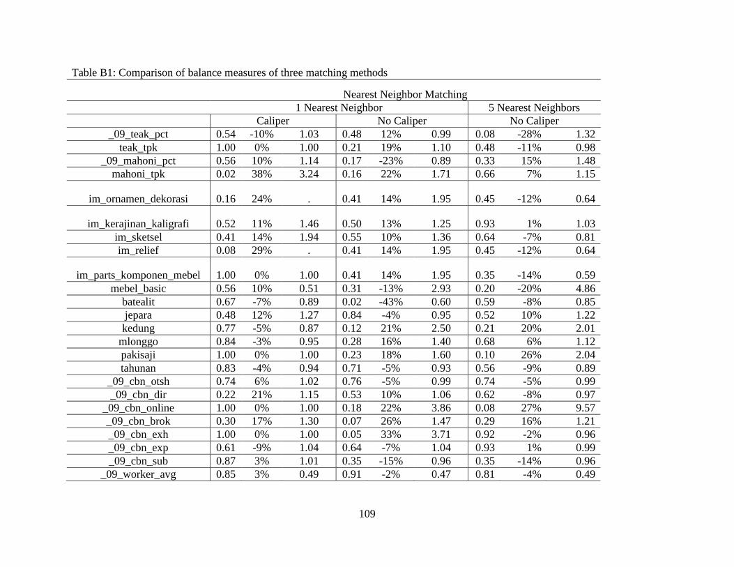
109





_09_teak_pct 0.54 -10% 1.03 0.48 12% 0.99 0.08 -28% 1.32

teak_tpk 1.00 0% 1.00 0.21 19% 1.10 0.48 -11% 0.98

_09_mahoni_pct 0.56 10% 1.14 0.17 -23% 0.89 0.33 15% 1.48

mahoni_tpk 0.02 38% 3.24 0.16 22% 1.71 0.66 7% 1.15

im_ornamen_dekorasi 0.16 24% . 0.41 14% 1.95 0.45 -12% 0.64

im_kerajinan_kaligrafi 0.52 11% 1.46 0.50 13% 1.25 0.93 1% 1.03

im_sketsel 0.41 14% 1.94 0.55 10% 1.36 0.64 -7% 0.81

im_relief 0.08 29% . 0.41 14% 1.95 0.45 -12% 0.64

im_parts_komponen_mebel 1.00 0% 1.00 0.41 14% 1.95 0.35 -14% 0.59

mebel_basic 0.56 10% 0.51 0.31 -13% 2.93 0.20 -20% 4.86

batealit 0.67 -7% 0.89 0.02 -43% 0.60 0.59 -8% 0.85

jepara 0.48 12% 1.27 0.84 -4% 0.95 0.52 10% 1.22

kedung 0.77 -5% 0.87 0.12 21% 2.50 0.21 20% 2.01

mlonggo 0.84 -3% 0.95 0.28 16% 1.40 0.68 6% 1.12

pakisaji 1.00 0% 1.00 0.23 18% 1.60 0.10 26% 2.04

tahunan 0.83 -4% 0.94 0.71 -5% 0.93 0.56 -9% 0.89

_09_cbn_otsh 0.74 6% 1.02 0.76 -5% 0.99 0.74 -5% 0.99

_09_cbn_dir 0.22 21% 1.15 0.53 10% 1.06 0.62 -8% 0.97

_09_cbn_online 1.00 0% 1.00 0.18 22% 3.86 0.08 27% 9.57

_09_cbn_brok 0.30 17% 1.30 0.07 26% 1.47 0.29 16% 1.21

_09_cbn_exh 1.00 0% 1.00 0.05 33% 3.71 0.92 -2% 0.96

_09_cbn_exp 0.61 -9% 1.04 0.64 -7% 1.04 0.93 1% 0.99

_09_cbn_sub 0.87 3% 1.01 0.35 -15% 0.96 0.35 -14% 0.96

_09_worker_avg 0.85 3% 0.49 0.91 -2% 0.47 0.81 -4% 0.49

110





_09_totalm2_workshop _sum 0.90 -2% 0.64 0.42 -14% 0.69 0.99 0% 0.81

_09_total_workshop 0.32 -17% 1.03 0.66 -6% . 0.73 -5% 25.00

_09_total _showroom 0.25 19% 2.39 0.05 25% 3.71 0.06 29% 3.38

_09_otherunits 0.55 10% 1.20 0.21 22% 1.57 0.35 15% 1.39

edu_sd 0.53 11% 1.19 0.56 -8% 0.87 0.70 -6% 0.91

edu_smp 0.72 6% 1.06 0.48 11% 1.14 0.55 9% 1.11

edu_stmsmk 1.00 0% 1.00 1.00 0% 1.00 0.92 -1% 0.92

edu_sma 0.48 -12% 0.91 0.73 6% 1.06 0.69 -6% 0.95

edu_high 0.65 -8% 0.86 0.86 -4% 0.96 0.71 6% 1.08

owner_age 0.92 2% 0.80 0.06 -30% 0.86 0.96 1% 0.88

Mean Bias 11.09% 15.40% 10.31%

Median Bias 9.74% 12.78% 8.44%


Appendix C: Stata Code Section 1 : Profit Estimation

Production (revenues)

*Avgprice*

egen avgprice1=rowmean(harganya_normal_01 harganya_low_01 harganya_high_01 harganya_4_01 harganya_5_01

harganya_6_01)

forvalues i=02/04{

egen avgpriceì'=rowmean(harganya_normal_0ì' harganya_low_0ì' harganya_high_0ì')

}

111

egen avgprice5=rowmean(harganya_normal_05 harganya_low_05 harganya_high_05 harganya_4_05)

egen avgprice6=rowmean(harganya_normal_06 harganya_low_06 harganya_high_06)

forvalues i=07/09{

gen avgpriceì'=harganya_normal_0ì'

}

forvalues i=10/15{

gen avgpriceì'=harganya_normal_ì'

}

//exceptions

replace avgprice1=( harganya_low_01 + harganya_high_01)/2 if count_id==504

*Avgjumlah, total_rec, comp_prod

egen avg_jumlah_prod_01=rowmean(jumlah_produksi_01 jum_prod_high jum_prod_low)

egen avgprice_all=rowmean(avgprice*)

*gen total_jumlah_no_dist (depends on case; should only exist for cases where distribution is not known)

*replace compare_prod=total_rec-avg_prod_l if seasonality_tabel_produksi==1

*replace compare_prod=total_rec-avg_prod_h if seasonality_tabel_produksi==3

egen total_rec=rowtotal(avg_jumlah_prod_01 jumlah_produksi_02 jumlah_produksi_03 jumlah_produksi_04

jumlah_produksi_05 jumlah_produksi_06 jumlah_produksi_07 jumlah_produksi_08 jumlah_produksi_09 jumlah_produksi_10

jumlah_produksi_11 jumlah_produksi_12)

*avg_total_nijual_

forvalues i=1/5{

egen avg_total_nijual_0ì'=rowmean(total_nijual_0ì' total_nijual_low_0ì' total_nijual_high_0ì')

}

*Roughrev_prod*

gen roughrev_prod1=avgprice1*avg_jumlah_prod_01

forvalues i=2/9{

gen roughrev_prodì'=avgpriceì'*jumlah_produksi_0ì'

}

forvalues i=10/11{

gen roughrev_prodì'=avgpriceì'*jumlah_produksi_ì'

112

}

gen roughrev_no_dist=total_jumlah_no_dist

//exceptions

replace roughrev_prod1 = avg_total_nijual_01 if roughrev_prod1==.





replace roughrev_prod6 = total_nijual_06 if roughrev_prod6==.



replace total_jumlah_no_dist=13 if count_id==459

replace total_jumlah_no_dist=100 if count_id==332

replace roughrev_no_dist=avgprice_all*total_jumlah_no_dist

*Roughrev_total

egen roughrev_total=rowtotal(roughrev_prod* roughrev_no_dist)

//exceptions

replace roughrev_total=roughrev_prod1 if count_id==504

replace roughrev_total=total_nijual_01 if count_id==554

*month_rev

g month_rev=roughrev_total if time_frame_prod==2

replace month_rev=roughrev_total*4 if time_frame_prod==1

gen year_rev=roughrev_total if time_frame_prod==3

label var year_rev "=roughrev_total if time_frame_prod==3"

//exceptions

replace month_rev=avg_total_nijual_01 if count_id==383


replace month_rev= (avg_total_nijual_02 + roughrev_prod1)*4 if count_id==43

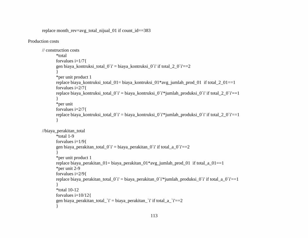
113


Production costs

// construction costs

*total

forvalues i=1/7{

gen biaya_kontruksi_total_0ì' = biaya_kontruksi_0ì' if total_2_0ì'==2

}

*per unit product 1

replace biaya_kontruksi_total_01= biaya_kontruksi_01*avg_jumlah_prod_01 if total_2_01==1

forvalues i=2/7{

replace biaya_kontruksi_total_0ì' = biaya_kontruksi_0ì'*jumlah_produksi_0ì' if total_2_0ì'==1

}

*per unit

forvalues i=2/7{

replace biaya_kontruksi_total_0ì' = biaya_kontruksi_0ì'*jumlah_produksi_0ì' if total_2_0ì'==1

}

//biaya_perakitan_total

*total 1-9

forvalues i=1/9{

gen biaya_perakitan_total_0ì' = biaya_perakitan_0ì' if total_a_0ì'==2

}

*per unit product 1

replace biaya_perakitan_01= biaya_perakitan_01*avg_jumlah_prod_01 if total_a_01==1

*per unit 2-9

forvalues i=2/9{

replace biaya_perakitan_total_0ì' = biaya_perakitan_0ì'*jumlah_produksi_0ì' if total_a_0ì'==1

}

*total 10-12

forvalues i=10/12{

gen biaya_perakitan_total_ì' = biaya_perakitan_ì' if total_a_ì'==2

}

114

*Per unit 10-12

forvalues i=10/12{

replace biaya_perakitan_total_ì' = biaya_perakitan_ì'*jumlah_produksi_ì' if total_a_ì'==1

}

//biaya_sanding_01

*per unit product 1

gen biaya_sanding_total_01= biaya_sanding_01*avg_jumlah_prod_01 if total_b_01==1

*per unit product 2

gen biaya_sanding_total_02= biaya_sanding_01*jumlah_produksi_02 if total_b_02==1

*total product 1

replace biaya_sanding_total_01= biaya_sanding_01 if total_a_01==2

*total product 2

replace biaya_sanding_total_02= biaya_sanding_01 if total_a_02==2

//biaya finishing

*total products 1-4

forvalues i=1/4{

gen biaya_finishing_total_0ì' = biaya_finishing_dikontrakan_0ì' if total_c_0ì'==2

}

*per unit product 1

replace biaya_finishing_total_01= biaya_finishing_dikontrakan_01*avg_jumlah_prod_01 if total_c_01==1

*per unit products 2-4

forvalues i=2/4{

replace biaya_finishing_total_0ì' = biaya_finishing_dikontrakan_0ì'*jumlah_produksi_0ì' if total_c_0ì'==1

}

*total products 2-4

forvalues i=2/4{

replace biaya_finishing_total_0ì' = biaya_finishing_dikontrakan_0ì' if total_c_0ì'==2

}

//no biaya_finishing_dikontrakan_05

*total products 6-7

forvalues i=6/7{

115

gen biaya_finishing_total_0ì' = biaya_finishing_dikontrakan_0ì' if total_c_0ì'==2

}

*Per unit products 6-7

forvalues i=6/7{

replace biaya_finishing_total_0ì' = biaya_finishing_dikontrakan_0ì'*jumlah_produksi_0ì' if total_c_0ì'==1

}

*Per unit product 1

replace biaya_finishing_total_01= biaya_finishing_dikontrakan_01*avg_jumlah_prod_01 if total_c_01==1

*Total products 6-7

forvalues i=6/7{

replace biaya_finishing_total_0ì' = biaya_finishing_dikontrakan_0ì' if total_c_0ì'==2

}

//produksi_costs_0

*prod costs 1-2

forvalues i=1/2{

egen produksi_costs_0ì' = rowtotal(biaya_finishing_total_0ì' biaya_sanding_total_0ì' biaya_perakitan_total_0ì'

biaya_kontruksi_total_0ì')

}

*prod costs 3-4

forvalues i=3/4{

egen produksi_costs_0ì' = rowtotal(biaya_finishing_total_0ì' biaya_perakitan_total_0ì' biaya_kontruksi_total_0ì')

}

*prod costs 5

egen produksi_costs_05 = rowtotal( biaya_perakitan_total_05 biaya_kontruksi_total_05)

*prod costs 6-7

forvalues i=6/7{

egen produksi_costs_0ì' = rowtotal(biaya_finishing_total_0ì' biaya_perakitan_total_0ì' biaya_kontruksi_total_0ì')

}

*prod costs 8-9

forvalues i=8/9{

116

egen produksi_costs_0ì' = rowtotal( biaya_perakitan_total_0ì')

}

*prod costs 10-12

forvalues i=10/12{

egen produksi_costs_ì' = rowtotal (biaya_perakitan_total_ì' )

}

//Produksi costs no jumlah

//Produksi

forvalues i=1/7{

gen perunit_konstruksi_0ì'=biaya_kontruksi_0ì' if total_2_01==1

}

egen avg_perunit_konstruksi=rowmean ( perunit_konstruksi_0*)

gen total_konstruksi_nodist=total_jumlah_no_dist*avg_perunit_konstruksi

//perakitan

forvalues i=2/9{

gen perunit_biaya_perakitan_0ì' = biaya_perakitan_0ì' if total_a_0ì'==1

}

forvalues i=10/12{

gen perunit_biaya_perakitan_ì' = biaya_perakitan_ì' if total_a_ì'==1

}

egen avg_perunit_perakitan=rowmean ( perunit_biaya_perakitan_0*)

gen total_perakitan_nodist=total_jumlah_no_dist*avg_perunit_perakitan

//sanding

gen perunit_sanding_01= biaya_sanding_01 if total_b_01==1

gen perunit_sanding_02= biaya_sanding_02 if total_b_02==2

117

egen avg_perunit_sanding=rowmean ( biaya_sanding_0*)

gen total_sanding_nodist=total_jumlah_no_dist*avg_perunit_sanding

//finishing

forvalues i=1/4{

gen perunit_finishing_0ì' = biaya_finishing_dikontrakan_0ì' if total_c_0ì'==1

}

forvalues i=6/7{

gen perunit_finishing_0ì' = biaya_finishing_dikontrakan_0ì' if total_c_0ì'==1

}

egen avg_perunit_finishing=rowmean ( biaya_finishing_*)

gen total_finishing_nodist=total_jumlah_no_dist*avg_perunit_finishing

//produksi no distribution

egen total_produksi_no_dist= rowtotal(total_konstruksi_nodist total_perakitan_nodist total_sanding_nodist

total_finishing_nodist)

//Aggregate production costs

egen total_costs_prod=rowtotal(total_produksi_no_dist produksi_costs_* borongan)

gen total_costs_prod_mo= total_costs_prod if time_frame_prod==2

replace total_costs_prod_mo= total_costs_prod*4 if time_frame_prod==1

gen total_costs_prod_yr= total_costs_prod if time_frame_prod==3

replace total_costs_prod_yr= 76410714 if count_id==425

replace total_costs_prod_mo=. if count_id==425

************************************************************************************

Wood Input Costs

//harga

egen avg_hargakayu_1= rowmean(harga_normal_1 harga_high_1 harga_low_1)

egen avg_hargakayu_2= rowmean(harga_normal_2 harga_high_2 harga_low_2)

//Kuantitas

118

egen avg_kuantitas_1= rowmean(kuantitas_normal_1 kuantitas_low_1 kuantitas_high_1)

//Oven

*m3 1

*truck 2

*pickup 3

*bilah 4

*borongan 5 (I considered it total)

*piece 6

*set 7

*natural 8

*other 9

*******************

*m3 1

gen total_oven_1=biaya_oven_1*avg_kuantitas_1 if biaya_oven_unit_1==1

gen total_oven_2=biaya_oven_2*kuantitas_normal_2 if biaya_oven_unit_2==1

gen total_oven_3=biaya_oven_3*kuantitas_normal_3 if biaya_oven_unit_3==1

*truck 2 made decision to assume total but IDK how much wood is in 1 truckload

replace total_oven_1=biaya_oven_1 if biaya_oven_unit_1==2

*borongan 5 (I considered it total)



*piece 6

replace total_oven_1=biaya_oven_1*jumlah_produksi_01 if biaya_oven_unit_1==6

*other 9

replace total_oven_1=biaya_oven_1*jumlah_produksi_01 if biaya_oven_unit_1==9

*not sure why I made that decision

//exceptions

119

replace total_oven_1=biaya_oven_1*avg_kuantitas_1 if count_id==509

replace total_oven_2=biaya_oven_2*kuantitas_normal_2 if count_id==509



replace total_oven_2=biaya_oven_2*kuantitas_normal_2 if count_id==509

//Sawmill 1

g total_bentuk_1=biaya_bentuk_log_1 if bentuk_log_unit_1==5

replace total_bentuk_1=biaya_bentuk_log_1*avg_kuantitas_1 if bentuk_log_unit_1==1

//exceptions

replace biaya_bentuk_log_1= 140000 if count_id==229

replace biaya_bentuk_log_1= 140000 if count_id==229

replace total_bentuk_1=biaya_bentuk_log_1 if count_id==229

replace total_bentuk_1=biaya_bentuk_log_1 if count_id==480|count_id==183|count_id==397

//Not sure about the pick up truck-how many pickup trucks is 7 m3 of wood?

//if the bed is 63 by 57.25 in. then there will be 12.6 m3 of room so I think I can assume that a truck bed is the total


//I think for the 9's I can assume that id 480 it is per unit and for id 183 it is total


replace total_bentuk_1=biaya_bentuk_log_1*kuantitas_normal_1 if count_id==581

replace total_bentuk_1=bentuk_log_unit_1*kuantitas_normal_1 if count_id==380

//*//*//*//*//*

replace avg_kuantitas_1=total_yang_dibayar_1/avg_hargakayu_1 if

count_id==531|count_id==167|count_id==50|count_id==334|count_id==385|count_id==525

//count_id=537 has quantity of 2-4

//*//*//*//*//*

//unit=9


gen total_bentuk_2=biaya_bentuk_log_2 if count_id==183

replace total_bentuk_1=biaya_bentuk_log_1*avg_kuantitas_1 if count_id==397|count_id==480

120



//Sawmill 2

replace total_bentuk_2=biaya_bentuk_log_2*kuantitas_normal_2 if bentuk_log_unit_2==1

replace total_bentuk_2=biaya_bentuk_log_2 if bentuk_log_unit_2==5

//Sawmill 3

gen total_bentuk_3=biaya_bentuk_log_3*kuantitas_normal_3 if bentuk_log_unit_3==1

replace total_bentuk_3=biaya_bentuk_log_3 if bentuk_log_unit_3==5

//Exceptions

//476: bentuk unit is missing. I think it is per unit so I will multiply by kuantitas


//480 bentuk unit missing. Assume per unit.


//183 assume total


//486 a challenge because there is harga per unit but quantity is missing

//checked questionnaire - 27 m3 must recalc avg_kuantitas forward

//total_wood_cost 1-4

gen total_wood_cost_1=avg_hargakayu_1*avg_kuantitas_1

replace total_wood_cost_1= total_yang_dibayar_1 if total_wood_cost_1==.

gen total_wood_cost_2= kuantitas_normal_2*avg_hargakayu_2

replace total_wood_cost_2=total_yang_dibayar_2 if total_wood_cost_2==.

gen total_wood_cost_3=kuantitas_normal_3*harga_normal_3

replace total_wood_cost_3= total_yang_dibayar_3 if total_wood_cost_3==.

gen total_wood_cost_4= kuantitas_normal_4*harga_normal_4

replace total_wood_cost_4=total_yang_dibayar_4 if total_wood_cost_4==.

// total wood costs all... by month... by year

egen total_wood_costs_all= rowtotal(total_wood_cost_1 total_wood_cost_2 total_wood_cost_3 total_wood_cost_4

total_oven_1 total_oven_2 total_oven_3 total_bentuk_1 total_bentuk_2 total_bentuk_3)

replace total_wood_costs_all=total_yang_dibayar_1 if count_id==237

121

replace total_wood_costs_all=total_yang_dibayar_1 + total_oven_1 + total_bentuk_1 if count_id==51

gen total_wood_costs_mo=total_wood_costs_all if time_frame_kayu==2

replace total_wood_costs_mo=total_wood_costs_all*4 if time_frame_kayu==1

gen total_wood_costs_yr=total_wood_costs_all if time_frame_kayu==3

//exceptions

replace total_wood_costs_yr=total_yang_dibayar_1 if count_id==574

Other Input Costs

*Bensin

gen avg_total_bensin=total_bensin

replace avg_total_bensin=jumlah_bensin*hpu_bensin_nor if total_bensin==.

gen month_bensin=avg_total_bensin if time_period_bensin==2

replace month_bensin=avg_total_bensin*4 if time_period_bensin==1

gen year_bensin=avg_total_bensin if time_period_bensin==3

*Solar

egen avg_total_solar= rowmean(total_solar total_solar_higi total_solar_low)

replace avg_total_solar=hpu_solar_normal*jumlah_solar if avg_total_solar==.

gen month_solar=avg_total_solar if time_period_solar==2

replace month_solar=avg_total_solar*4 if time_period_solar==1

gen year_solar=avg_total_solar if time_period_solar==3

*Listrik

gen calc_total_listrik_high=hpu_listrik_high*jumlah_listrik if total_listrik_high==.

gen calc_total_listrik=hpu_listrik_normal*jumlah_listrik if total_listrik==.

gen calc_total_listrik_low=hpu_listrik_low*jumlah_listrik if total_listrik_low==.

egen avg_total_listrik= rowmean(total_listrik total_listrik_high total_listrik_low calc_total_listrik_low calc_total_listrik

calc_total_listrik_high)

122

gen month_listrik=avg_total_listrik if time_period_listrik==2

replace month_listrik=avg_total_listrik*4 if time_period_listrik==1

gen year_listrik=avg_total_listrik if time_period_listrik==3

*Transportation

egen avg_total_trans=rowmean(total_transportasi total_trans_high total_trans_low)

replace avg_total_trans=hpu_transportasi_normal*jumlah_transportasi if avg_total_trans==.

gen month_trans=avg_total_trans if time_period_trans==2

replace month_trans=avg_total_trans*4 if time_period_trans==1

gen year_trans=avg_total_trans if time_period_trans==3

*Finish

gen avg_total_finish=total_finish

replace avg_total_finish=harga_per_uniy*jumlah_finishing if total_finish==.

gen month_finish=avg_total_finish if time_period_finish==2

replace month_finish=avg_total_finish*4 if time_period_finish==1

gen year_finish=avg_total_finish if time_period_finish==3

//Aggregate other costs

egen total_costs_other= rowtotal(month_trans month_listrik month_solar month_bensin month_finish)

egen total_costs_other_yr= rowtotal(year_trans year_listrik year_solar year_finish)

Labor Input Costs

//Women

egen avg_wage_f= rowmean (wage_f_normal_1 wage_f_high_1 wage_f_low_1)

//by week per person

gen month_wage_f=avg_wage_f*4 if dibayaran_per_1==2 & per_or_total_1==1

//by week total jumlah

replace month_wage_f=(avg_wage_f/jumlah_perempuan_1)*4 if dibayaran_per_1==2 & per_or_total_1==2

123

//by day total jumlah

replace month_wage_f=(avg_wage_f/jumlah_perempuan_1)*24 if dibayaran_per_1==1 & per_or_total_1==2

//by day per person

replace month_wage_f=(avg_wage_f)*24 if dibayaran_per_1==1 & per_or_total_1==1

//by month total jumlah

replace month_wage_f=avg_wage_f/jumlah_perempuan_1 if dibayaran_per_1==3 & per_or_total_1==2

//by month per person

replace month_wage_f=avg_wage_f if dibayaran_per_1==3 & per_or_total_1==1

//MEN

egen avg_wage_m= rowmean (wage_m_normal_1 wage_m_high_1 wage_m_low_1)

//by week per person

gen month_wage_m=avg_wage_m*4 if dibayaran_per_1==2 & per_or_total_1==1

//by week total jumlah

replace month_wage_m=(avg_wage_m/jumlah_laki_laki_1)*4 if dibayaran_per_1==2 & per_or_total_1==2

//by day total jumlah

replace month_wage_m=(avg_wage_m/jumlah_laki_laki_1)*24 if dibayaran_per_1==1 & per_or_total_1==2

//by day per person

replace month_wage_m=(avg_wage_m)*24 if dibayaran_per_1==1 & per_or_total_1==1

//by month total jumlah

replace month_wage_m=avg_wage_m/jumlah_laki_laki_1 if dibayaran_per_1==3 & per_or_total_1==2

//by month per person

replace month_wage_m=avg_wage_m if dibayaran_per_1==3 & per_or_total_1==1

//Neutral and production wages

gen prod_wage=total_rec*avg_wage_m if dibayaran_per_1==4 & avg_wage_m!=. & avg_wage_m!=0|dibayaran_per_1==5 &

avg_wage_m!=. & avg_wage_m!=0

replace prod_wage=avg_wage_m*(jumlah_laki_laki_1+jumlah_perempuan_1) if count_id==152

gen prod_wage_mo=prod_wage if time_frame_prod==2

replace prod_wage_mo=prod_wage*4 if time_frame_prod==1

124

//Missing women's wages

replace prop_replace_f_wage=.5443311*month_wage_m if avg_wage_f==. & jumlah_perempuan_1!=. &

jumlah_perempuan_1!=0 & dibayaran_per_1==1 |avg_wage_f==. & jumlah_perempuan_1!=. & jumlah_perempuan_1!=0 &

dibayaran_per_1==2 |avg_wage_f==. & jumlah_perempuan_1!=. & jumlah_perempuan_1!=0 & dibayaran_per_1==3

replace mean_replace_f_wage=822654.2 if avg_wage_f==. & jumlah_perempuan_1!=. & jumlah_perempuan_1!=0 &

dibayaran_per_1==1 |avg_wage_f==. & jumlah_perempuan_1!=. & jumlah_perempuan_1!=0 & dibayaran_per_1==2 |avg_wage_f==.

& jumlah_perempuan_1!=. & jumlah_perempuan_1!=0 & dibayaran_per_1==3

replace prop_mode_replace_f_wage=.4761905 *month_wage_m if avg_wage_f==. & jumlah_perempuan_1!=. &



replace total_wage_f_missing_propmean=prop_replace_f_wage*jumlah_perempuan_1

replace total_wage_f_missing_propmode=prop_mode_replace_f_wage*jumlah_perempuan_1

replace total_wage_f_missing_mean=745310.7*jumlah_perempuan_1 if avg_wage_f==. & jumlah_perempuan_1!=. &



sum month_wage_f, detail

*IQR 266666.7

*Upper bound 1266666.75

*Lower bound -199999.95

sum month_wage_f if month_wage_f<1266666.75, detail

*mean: 745310.7

//Aggregate wages further

gen total_wage_f=month_wage_f*jumlah_perempuan_1

gen total_wage_m=month_wage_m*jumlah_laki_laki_1

egen total_labor_mo = rowtotal (total_dibayar_pekerja_1 prod_wage_mo total_wage_m total_wage_f total_wage_f_missing_mean)

//Total Costs

125

*drop total_costs_mo total_costs_yr

egen total_costs_mo=rowtotal( total_labor_mo total_wood_costs_mo total_costs_other total_costs_prod_mo)

egen total_costs_yr=rowtotal(total_wood_costs_yr total_costs_other_yr total_costs_prod_yr)

egen total_costs_mo_nl_nw=rowtotal(total_costs_other total_costs_prod_mo)

//Seasonality

gen augprod_n=augprod if aug123==2

gen sepprod_n=sepprod if sep123==2

gen octprod_n=octprod if oct123==2

gen novprod_n=novprod if nov123==2

gen decprod_n=decprod if dec123==2

gen janprod_n=janprod if jan123==2

gen febprod_n=febprod if feb123==2

gen marprod_n=marprod if mar123==2

gen aprprod_n=aprprod if apr123==2

gen mayprod_n=mayprod if may123==2

gen junprod_n=junprod if jun123==2

gen julprod_n=julprod if jul123==2

replace augprod_l=augprod if aug123==1

replace sepprod_l=sepprod if sep123==1

replace octprod_l=octprod if oct123==1

replace novprod_l=novprod if nov123==1

replace decprod_l=decprod if dec123==1

replace janprod_l=janprod if jan123==1

replace febprod_l=febprod if feb123==1

replace marprod_l=marprod if mar123==1

replace aprprod_l=aprprod if apr123==1

replace mayprod_l=mayprod if may123==1

replace junprod_l=junprod if jun123==1

replace julprod_l=julprod if jul123==1

126

replace augprod_h=augprod if aug123==3

replace sepprod_h=sepprod if sep123==3

replace octprod_h=octprod if oct123==3

replace novprod_h=novprod if nov123==3

replace decprod_h=decprod if dec123==3

replace janprod_h=janprod if jan123==3

replace febprod_h=febprod if feb123==3

replace marprod_h=marprod if mar123==3

replace aprprod_h=aprprod if apr123==3

replace mayprod_h=mayprod if may123==3

replace junprod_h=junprod if jun123==3

replace julprod_h=julprod if jul123==3

egen avg_prod_h=rowmean(augprod_h-julprod_h)

egen avg_prod_l=rowmean(augprod_l-julprod_l)

egen avg_prod_n=rowmean(augprod_n-julprod_n)

*Monthly scale

gen aug_scale=augprod/avg_prod_n if seasonality_tabel_produksi==2

gen sep_scale=sepprod/avg_prod_n if seasonality_tabel_produksi==2

gen oct_scale=octprod/avg_prod_n if seasonality_tabel_produksi==2

gen nov_scale=novprod/avg_prod_n if seasonality_tabel_produksi==2

gen dec_scale=decprod/avg_prod_n if seasonality_tabel_produksi==2

gen jan_scale=janprod/avg_prod_n if seasonality_tabel_produksi==2

gen feb_scale=febprod/avg_prod_n if seasonality_tabel_produksi==2

gen mar_scale=marprod/avg_prod_n if seasonality_tabel_produksi==2

gen apr_scale=aprprod/avg_prod_n if seasonality_tabel_produksi==2

gen may_scale=mayprod/avg_prod_n if seasonality_tabel_produksi==2

gen jun_scale=junprod/avg_prod_n if seasonality_tabel_produksi==2

gen jul_scale=julprod/avg_prod_n if seasonality_tabel_produksi==2

127

replace aug_scale=augprod/avg_prod_h if seasonality_tabel_produksi==3

replace sep_scale=sepprod/avg_prod_h if seasonality_tabel_produksi==3

replace oct_scale=octprod/avg_prod_h if seasonality_tabel_produksi==3

replace nov_scale=novprod/avg_prod_h if seasonality_tabel_produksi==3

replace dec_scale=decprod/avg_prod_h if seasonality_tabel_produksi==3

replace jan_scale=janprod/avg_prod_h if seasonality_tabel_produksi==3

replace feb_scale=febprod/avg_prod_h if seasonality_tabel_produksi==3

replace mar_scale=marprod/avg_prod_h if seasonality_tabel_produksi==3

replace apr_scale=aprprod/avg_prod_h if seasonality_tabel_produksi==3

replace may_scale=mayprod/avg_prod_h if seasonality_tabel_produksi==3

replace jun_scale=junprod/avg_prod_h if seasonality_tabel_produksi==3

replace jul_scale=julprod/avg_prod_h if seasonality_tabel_produksi==3

replace aug_scale=augprod/avg_prod_l if seasonality_tabel_produksi==1

replace sep_scale=sepprod/avg_prod_l if seasonality_tabel_produksi==1

replace oct_scale=octprod/avg_prod_l if seasonality_tabel_produksi==1

replace nov_scale=novprod/avg_prod_l if seasonality_tabel_produksi==1

replace dec_scale=decprod/avg_prod_l if seasonality_tabel_produksi==1

replace jan_scale=janprod/avg_prod_l if seasonality_tabel_produksi==1

replace feb_scale=febprod/avg_prod_l if seasonality_tabel_produksi==1

replace mar_scale=marprod/avg_prod_l if seasonality_tabel_produksi==1

replace apr_scale=aprprod/avg_prod_l if seasonality_tabel_produksi==1

replace may_scale=mayprod/avg_prod_l if seasonality_tabel_produksi==1

replace jun_scale=junprod/avg_prod_l if seasonality_tabel_produksi==1

replace jul_scale=julprod/avg_prod_l if seasonality_tabel_produksi==1

replace sep_scale=0 if sepprod==0

replace oct_scale=0 if octprod==0

replace nov_scale=0 if novprod==0

replace dec_scale=0 if decprod==0

replace jan_scale=0 if janprod==0

replace feb_scale=0 if febprod==0

128

replace mar_scale=0 if marprod==0

replace apr_scale=0 if aprprod==0

replace may_scale=0 if mayprod==0

replace jun_scale=0 if junprod==0

replace jul_scale=0 if julprod==0

//Labor Scale

replace seasonal_labor=1 if _15_worker_ramai!=_15_worker_normal & _15_worker_ramai!=. & _15_worker_normal!=.

|_15_worker_sepi!=_15_worker_normal & _15_worker_sepi!=. & _15_worker_normal!=.

replace seasonal_labor=0 if _15_worker_ramai==_15_worker_normal & _15_worker_normal==_15_worker_sepi

label var seasonal_labor_yn "Whether there are seasonal differences in labor; 1=yes"

egen total_workers=rowtotal(jumlah_tenaga_kerja_1 jumlah_tenaga_kerja_2)

replace season_labor_table = 1 if total_workers==_15_worker_sepi

replace season_labor_table = 2 if total_workers==_15_worker_normal

replace season_labor_table = 3 if total_workers==_15_worker_ramai

replace season_labor_table = 2 if total_workers==_15_worker_normal==_15_worker_sepi==_15_worker_ramai

label var season_labor_table "The season that the worker table fits with based on _15_worker_normal _15_worker_sepi

_15_worker_ramai"

replace season_labor_table = 2 if count_id==249










gen ltn=_15_worker_normal/_15_worker_sepi

129

gen lth=_15_worker_ramai/_15_worker_sepi

gen ntl=_15_worker_sepi/_15_worker_normal

gen nth=_15_worker_ramai/_15_worker_normal

gen htl=_15_worker_sepi/_15_worker_ramai

gen htn=_15_worker_normal/_15_worker_ramai

//August

gen aug_labor_scale=1 if season_labor_table==1 & aug123==1

replace aug_labor_scale=ntl if season_labor_table==2 & aug123==1

replace aug_labor_scale=htl if season_labor_table==3 & aug123==1

replace aug_labor_scale=ltn if season_labor_table==1 & aug123==2

replace aug_labor_scale=1 if season_labor_table==2 & aug123==2

replace aug_labor_scale=htn if season_labor_table==3 & aug123==2

replace aug_labor_scale=lth if season_labor_table==1 & aug123==3

replace aug_labor_scale=nth if season_labor_table==2 & aug123==3

replace aug_labor_scale=1 if season_labor_table==3 & aug123==3

**********************

//September

gen sep_labor_scale=1 if season_labor_table==1 & sep123==1

replace sep_labor_scale=ntl if season_labor_table==2 & sep123==1

replace sep_labor_scale=htl if season_labor_table==3 & sep123==1

replace sep_labor_scale=ltn if season_labor_table==1 & sep123==2

replace sep_labor_scale=1 if season_labor_table==2 & sep123==2

replace sep_labor_scale=htn if season_labor_table==3 & sep123==2

replace sep_labor_scale=lth if season_labor_table==1 & sep123==3

replace sep_labor_scale=nth if season_labor_table==2 & sep123==3

130

replace sep_labor_scale=1 if season_labor_table==3 & sep123==3

*************************

//October

gen oct_labor_scale=1 if season_labor_table==1 & oct123==1

replace oct_labor_scale=ntl if season_labor_table==2 & oct123==1

replace oct_labor_scale=htl if season_labor_table==3 & oct123==1

replace oct_labor_scale=ltn if season_labor_table==1 & oct123==2

replace oct_labor_scale=1 if season_labor_table==2 & oct123==2

replace oct_labor_scale=htn if season_labor_table==3 & oct123==2

replace oct_labor_scale=lth if season_labor_table==1 & oct123==3

replace oct_labor_scale=nth if season_labor_table==2 & oct123==3

replace oct_labor_scale=1 if season_labor_table==3 & oct123==3

*****************************

//November

gen nov_labor_scale=1 if season_labor_table==1 & nov123==1

replace nov_labor_scale=ntl if season_labor_table==2 & nov123==1

replace nov_labor_scale=htl if season_labor_table==3 & nov123==1

replace nov_labor_scale=ltn if season_labor_table==1 & nov123==2

replace nov_labor_scale=1 if season_labor_table==2 & nov123==2

replace nov_labor_scale=htn if season_labor_table==3 & nov123==2

replace nov_labor_scale=lth if season_labor_table==1 & nov123==3

replace nov_labor_scale=nth if season_labor_table==2 & nov123==3

replace nov_labor_scale=1 if season_labor_table==3 & nov123==3

****************************

////December

gen dec_labor_scale=1 if season_labor_table==1 & dec123==1

replace dec_labor_scale=ntl if season_labor_table==2 & dec123==1

replace dec_labor_scale=htl if season_labor_table==3 & dec123==1

131

replace dec_labor_scale=ltn if season_labor_table==1 & dec123==2

replace dec_labor_scale=1 if season_labor_table==2 & dec123==2

replace dec_labor_scale=htn if season_labor_table==3 & dec123==2

replace dec_labor_scale=lth if season_labor_table==1 & dec123==3

replace dec_labor_scale=nth if season_labor_table==2 & dec123==3

replace dec_labor_scale=1 if season_labor_table==3 & dec123==3

****************************

////January

gen jan_labor_scale=1 if season_labor_table==1 & jan123==1

replace jan_labor_scale=ntl if season_labor_table==2 & jan123==1

replace jan_labor_scale=htl if season_labor_table==3 & jan123==1

replace jan_labor_scale=ltn if season_labor_table==1 & jan123==2

replace jan_labor_scale=1 if season_labor_table==2 & jan123==2

replace jan_labor_scale=htn if season_labor_table==3 & jan123==2

replace jan_labor_scale=lth if season_labor_table==1 & jan123==3

replace jan_labor_scale=nth if season_labor_table==2 & jan123==3

replace jan_labor_scale=1 if season_labor_table==3 & jan123==3

****************************

////February

gen feb_labor_scale=1 if season_labor_table==1 & feb123==1

replace feb_labor_scale=ntl if season_labor_table==2 & feb123==1

replace feb_labor_scale=htl if season_labor_table==3 & feb123==1

replace feb_labor_scale=ltn if season_labor_table==1 & feb123==2

replace feb_labor_scale=1 if season_labor_table==2 & feb123==2

replace feb_labor_scale=htn if season_labor_table==3 & feb123==2

replace feb_labor_scale=lth if season_labor_table==1 & feb123==3

replace feb_labor_scale=nth if season_labor_table==2 & feb123==3

132

replace feb_labor_scale=1 if season_labor_table==3 & feb123==3

****************************

//March

gen mar_labor_scale=1 if season_labor_table==1 & mar123==1

replace mar_labor_scale=ntl if season_labor_table==2 & mar123==1

replace mar_labor_scale=htl if season_labor_table==3 & mar123==1

replace mar_labor_scale=ltn if season_labor_table==1 & mar123==2

replace mar_labor_scale=1 if season_labor_table==2 & mar123==2

replace mar_labor_scale=htn if season_labor_table==3 & mar123==2

replace mar_labor_scale=lth if season_labor_table==1 & mar123==3

replace mar_labor_scale=nth if season_labor_table==2 & mar123==3

replace mar_labor_scale=1 if season_labor_table==3 & mar123==3

******************************

//April

gen apr_labor_scale=1 if season_labor_table==1 & apr123==1

replace apr_labor_scale=ntl if season_labor_table==2 & apr123==1

replace apr_labor_scale=htl if season_labor_table==3 & apr123==1

replace apr_labor_scale=ltn if season_labor_table==1 & apr123==2

replace apr_labor_scale=1 if season_labor_table==2 & apr123==2

replace apr_labor_scale=htn if season_labor_table==3 & apr123==2

replace apr_labor_scale=lth if season_labor_table==1 & apr123==3

replace apr_labor_scale=nth if season_labor_table==2 & apr123==3

replace apr_labor_scale=1 if season_labor_table==3 & apr123==3

*****************************

//May

gen may_labor_scale=1 if season_labor_table==1 & may123==1

replace may_labor_scale=ntl if season_labor_table==2 & may123==1

replace may_labor_scale=htl if season_labor_table==3 & may123==1

133

replace may_labor_scale=ltn if season_labor_table==1 & may123==2

replace may_labor_scale=1 if season_labor_table==2 & may123==2

replace may_labor_scale=htn if season_labor_table==3 & may123==2

replace may_labor_scale=lth if season_labor_table==1 & may123==3

replace may_labor_scale=nth if season_labor_table==2 & may123==3

replace may_labor_scale=1 if season_labor_table==3 & may123==3

****************************

//June

gen jun_labor_scale=1 if season_labor_table==1 & jun123==1

replace jun_labor_scale=ntl if season_labor_table==2 & jun123==1

replace jun_labor_scale=htl if season_labor_table==3 & jun123==1

replace jun_labor_scale=ltn if season_labor_table==1 & jun123==2

replace jun_labor_scale=1 if season_labor_table==2 & jun123==2

replace jun_labor_scale=htn if season_labor_table==3 & jun123==2

replace jun_labor_scale=lth if season_labor_table==1 & jun123==3

replace jun_labor_scale=nth if season_labor_table==2 & jun123==3

replace jun_labor_scale=1 if season_labor_table==3 & jun123==3

****************************

//July

gen jul_labor_scale=1 if season_labor_table==1 & jul123==1

replace jul_labor_scale=ntl if season_labor_table==2 & jul123==1

replace jul_labor_scale=htl if season_labor_table==3 & jul123==1

replace jul_labor_scale=ltn if season_labor_table==1 & jul123==2

replace jul_labor_scale=1 if season_labor_table==2 & jul123==2

replace jul_labor_scale=htn if season_labor_table==3 & jul123==2

replace jul_labor_scale=lth if season_labor_table==1 & jul123==3

replace jul_labor_scale=nth if season_labor_table==2 & jul123==3

replace jul_labor_scale=1 if season_labor_table==3 & jul123==3

134

****************************

replace aug_labor=aug_labor_scale*total_labor

replace sep_labor=sep_labor_scale*total_labor

replace oct_labor=oct_labor_scale*total_labor

replace nov_labor=nov_labor_scale*total_labor

replace dec_labor=dec_labor_scale*total_labor

replace jan_labor=jan_labor_scale*total_labor

replace feb_labor=feb_labor_scale*total_labor

replace mar_labor=mar_labor_scale*total_labor

replace apr_labor=apr_labor_scale*total_labor

replace may_labor=may_labor_scale*total_labor

replace jun_labor=jun_labor_scale*total_labor

replace jul_labor=jul_labor_scale*total_labor

//Scale Exceptions

//531

replace aug_scale=1 if count_id==531

replace sep_scale=1 if count_id==531

replace oct_scale=1 if count_id==531

replace nov_scale=1 if count_id==531

replace dec_scale=1 if count_id==531

replace jan_scale=1 if count_id==531

replace feb_scale=1 if count_id==531

replace mar_scale=1 if count_id==531

replace apr_scale=1 if count_id==531

replace may_scale=1 if count_id==531

replace jun_scale=1 if count_id==531

replace jul_scale=1 if count_id==531

//464





135









//449













//523


replace sep123=2 if count_id==523


replace oct123 =2 if count_id==523

replace oct_scale =1 if count_id==523

replace nov123 =2 if count_id==523

replace nov_scale =1 if count_id==523

*******

replace dec123 =3 if count_id==523

136

replace dec_scale =1.5 if count_id==523

replace jan123 =3 if count_id==523

replace jan_scale =1.5 if count_id==523

replace feb123 =3 if count_id==523

replace feb_scale =1.5 if count_id==523

*********

replace mar123 =2 if count_id==523

replace mar_scale =1 if count_id==523

replace apr123 =2 if count_id==523

replace apr_scale =1 if count_id==523

replace may123 =2 if count_id==523

replace may_scale =1 if count_id==523

replace jun123 =2 if count_id==523


replace jul123=2 if count_id==523


//131












//82




137










//489









replace dec_scale =1 if count_id==489


replace jan_scale =1 if count_id==489


replace feb_scale =1 if count_id==489










138


//504













//538








*******


replace dec_scale =dec_labor_scale if count_id==538


replace jan_scale =jan_labor_scale if count_id==538


replace feb_scale =feb_labor_scale if count_id==538

139

*********











//554













//450


replace sep_scale=sep_labor_scale if count_id==450


replace oct_scale=oct_labor_scale if count_id==450

140

****


replace novprod =40 if count_id==450

*****


replace dec_scale=dec_labor_scale if count_id==450


replace jan_scale=jan_labor_scale if count_id==450



*****


replace marprod =40 if count_id==450


replace aprprod =40 if count_id==450


replace mayprod =40 if count_id==450


replace junprod=40 if count_id==450


replace julprod=40 if count_id==450

//461

replace aug_scale=.4 if count_id==461

replace sep_scale=.4 if count_id==461

replace oct_scale=.4 if count_id==461

replace nov_scale=.4 if count_id==461

replace dec_scale=.4 if count_id==461

replace jan_scale=.4 if count_id==461



replace apr_scale=.4 if count_id==461

replace may_scale=.67 if count_id==461

141



//51







replace feb_scale=feb_labor_scale if count_id==51

replace mar_scale=mar_labor_scale if count_id==51

replace apr_scale=apr_labor_scale if count_id==51

replace may_scale= may_labor_scale if count_id==51

replace jun_scale=jun_labor_scale if count_id==51

replace jul_scale=jul_labor_scale if count_id==51

//420


replace sep_scale=sep_labor_scale if count_id==420


replace oct_scale=oct_labor_scale if count_id==420

*****

*****







//17

142

replace aug_scale =1 if count_id==17

replace sep_scale =1 if count_id==17



replace dec_scale =1 if count_id==17

replace jan_scale =1 if count_id==17

replace feb_scale =1 if count_id==17




replace jun_scale =1 if count_id==17

replace jul_scale =1 if count_id==17

//Scale to year

replace aug_costs=total_costs_mo*aug_scale

replace sep_costs=total_costs_mo*sep_scale

replace oct_costs=total_costs_mo*oct_scale

replace nov_costs=total_costs_mo*nov_scale

replace dec_costs=total_costs_mo*dec_scale

replace jan_costs=total_costs_mo*jan_scale

replace feb_costs=total_costs_mo*feb_scale

replace mar_costs=total_costs_mo*mar_scale

replace apr_costs=total_costs_mo*apr_scale

replace may_costs=total_costs_mo*may_scale

replace jun_costs=total_costs_mo*jun_scale

replace jul_costs=total_costs_mo*jul_scale

egen year_costs_original=rowtotal(total_costs_yr aug_costs sep_costs oct_costs nov_costs dec_costs jan_costs feb_costs

mar_costs apr_costs may_costs jun_costs jul_costs)

replace aug_rev=month_rev*aug_scale

replace sep_rev=month_rev*sep_scale

replace oct_rev=month_rev*oct_scale

143

replace nov_rev=month_rev*nov_scale

replace dec_rev=month_rev*dec_scale

replace jan_rev=month_rev*jan_scale

replace feb_rev=month_rev*feb_scale

replace mar_rev=month_rev*mar_scale

replace apr_rev=month_rev*apr_scale

replace may_rev=month_rev*may_scale

replace jun_rev=month_rev*jun_scale

replace jul_rev=month_rev*jul_scale

egen year_rev_total=rowtotal(year_rev aug_rev sep_rev oct_rev nov_rev dec_rev jan_rev feb_rev mar_rev apr_rev may_rev

jun_rev jul_rev)

note year_rev_total:year_rev aug_rev sep_rev oct_rev nov_rev dec_rev jan_rev feb_rev mar_rev apr_rev may_rev jun_rev

jul_rev

replace year_rev_total= 97250000 if count_id==425

//No labor no wood

replace aug_costs_nl_nw=total_costs_mo_nl_nw*aug_scale

replace sep_costs_nl_nw=total_costs_mo_nl_nw*sep_scale

replace oct_costs_nl_nw=total_costs_mo_nl_nw*oct_scale

replace nov_costs_nl_nw=total_costs_mo_nl_nw*nov_scale

replace dec_costs_nl_nw=total_costs_mo_nl_nw*dec_scale

replace jan_costs_nl_nw=total_costs_mo_nl_nw*jan_scale

replace feb_costs_nl_nw=total_costs_mo_nl_nw*feb_scale

replace mar_costs_nl_nw=total_costs_mo_nl_nw*mar_scale

replace apr_costs_nl_nw=total_costs_mo_nl_nw*apr_scale

replace may_costs_nl_nw=total_costs_mo_nl_nw*may_scale

replace jun_costs_nl_nw=total_costs_mo_nl_nw*jun_scale

replace jul_costs_nl_nw=total_costs_mo_nl_nw*jul_scale

144

////Alternative wood quantity

g scale_down_1=alt_kuantitas_normal_1/avg_kuantitas_1

g scale_down_2=alt_kuantitas_normal_2/kuantitas_normal_2

g alt_total_oven_1=biaya_oven_1*alt_kuantitas_normal_1 if biaya_oven_unit_1==1 & alt_kuantitas_normal_1!=.

replace alt_total_oven_1=biaya_oven_1*scale_down_1 if biaya_oven_unit_1==5 & alt_kuantitas_normal_1!=.

g alt_total_oven_2=biaya_oven_2*alt_kuantitas_normal_1 if biaya_oven_unit_1==1 & alt_kuantitas_normal_1!=.

replace alt_total_oven_2=biaya_oven_2*scale_down_2 if biaya_oven_unit_2==5 & alt_kuantitas_normal_2!=.

g alt_total_bentuk_1=biaya_bentuk_log_1*scale_down_1 if bentuk_log_unit_1==5 & alt_kuantitas_normal_1!=.

replace alt_total_bentuk_1=biaya_bentuk_log_1*alt_kuantitas_normal_1 if bentuk_log_unit_1==1 &

alt_kuantitas_normal_1!=.

g alt_total_bentuk_2=biaya_bentuk_log_2*scale_down_2 if bentuk_log_unit_2==5 & alt_kuantitas_normal_2!=.

replace alt_total_bentuk_2=biaya_bentuk_log_2*alt_kuantitas_normal_2 if bentuk_log_unit_2==1 &

alt_kuantitas_normal_2!=.

g alt_total_wood_cost_1=avg_hargakayu_1*alt_kuantitas_normal_1

g alt_total_wood_cost_2=avg_hargakayu_2*alt_kuantitas_normal_2

egen alt_total_wood_costs_all= rowtotal(alt_total_wood_cost_1 alt_total_oven_1 alt_total_bentuk_1 alt_total_wood_cost_2

alt_total_oven_2 alt_total_bentuk_2)

replace alt_total_wood_costs_all=. if alt_kuantitas_normal_1==.

gen alt_total_wood_costs_mo=alt_total_wood_costs_all if time_frame_kayu==2 & alt_total_wood_costs_all!=.

replace alt_total_wood_costs_mo=alt_total_wood_costs_all*4 if time_frame_kayu==1 & alt_total_wood_costs_all!=.

gen alt_total_wood_costs_yr=alt_total_wood_costs_all if time_frame_kayu==3 & alt_total_wood_costs_all!=.

replace aug_alt_wood_costs=alt_total_wood_costs_mo*aug_scale if alt_total_wood_costs_all!=.

replace sep_alt_wood_costs=alt_total_wood_costs_mo*sep_scale if alt_total_wood_costs_all!=.

replace oct_alt_wood_costs=alt_total_wood_costs_mo*oct_scale if alt_total_wood_costs_all!=.

145

replace nov_alt_wood_costs=alt_total_wood_costs_mo*nov_scale if alt_total_wood_costs_all!=.

replace dec_alt_wood_costs=alt_total_wood_costs_mo*dec_scale if alt_total_wood_costs_all!=.

replace jan_alt_wood_costs=alt_total_wood_costs_mo*jan_scale if alt_total_wood_costs_all!=.

replace feb_alt_wood_costs=alt_total_wood_costs_mo*feb_scale if alt_total_wood_costs_all!=.

replace mar_alt_wood_costs=alt_total_wood_costs_mo*mar_scale if alt_total_wood_costs_all!=.

replace apr_alt_wood_costs=alt_total_wood_costs_mo*apr_scale if alt_total_wood_costs_all!=.

replace may_alt_wood_costs=alt_total_wood_costs_mo*may_scale if alt_total_wood_costs_all!=.

replace jun_alt_wood_costs=alt_total_wood_costs_mo*jun_scale if alt_total_wood_costs_all!=.

replace jul_alt_wood_costs=alt_total_wood_costs_mo*jul_scale if alt_total_wood_costs_all!=.

drop year_alt_wood_costs

egen year_alt_wood_costs=rowtotal(alt_total_wood_costs_yr aug_alt_wood_costs sep_alt_wood_costs oct_alt_wood_costs

nov_alt_wood_costs dec_alt_wood_costs jan_alt_wood_costs feb_alt_wood_costs mar_alt_wood_costs jun_alt_wood_costs

jul_alt_wood_costs)

****************************************************************

//Profit Calculations

//Non-seasonal labor and without alternative wood

drop year_profit_original year_profit_original_dollars

gen year_profit_original=year_rev_total-year_costs_original

replace year_profit_original=. if year_profit_original==0 & year_rev_total==0 & year_costs_original==0

gen year_profit_original_dollars=year_profit_original/12500

//Seasonal Labor without alternative wood

egen total_costs_season_labor=rowtotal(aug_labor sep_labor oct_labor nov_labor dec_labor jan_labor feb_labor mar_labor

apr_labor may_labor jun_labor jul_labor)

egen total_costs_mo_nolabor=rowtotal(total_wood_costs_mo total_costs_other total_costs_prod_mo )

146

egen total_costs_yr_nolabor=rowtotal(total_wood_costs_yr total_costs_other_yr total_costs_prod_yr )

replace aug_costs_nl=total_costs_mo_nolabor*aug_scale

replace sep_costs_nl=total_costs_mo_nolabor*sep_scale

replace oct_costs_nl=total_costs_mo_nolabor*oct_scale

replace nov_costs_nl=total_costs_mo_nolabor*nov_scale

replace dec_costs_nl=total_costs_mo_nolabor*dec_scale

replace jan_costs_nl=total_costs_mo_nolabor*jan_scale

replace feb_costs_nl=total_costs_mo_nolabor*feb_scale

replace mar_costs_nl=total_costs_mo_nolabor*mar_scale

replace apr_costs_nl=total_costs_mo_nolabor*apr_scale

replace may_costs_nl=total_costs_mo_nolabor*may_scale

replace jun_costs_nl=total_costs_mo_nolabor*jun_scale

replace jul_costs_nl=total_costs_mo_nolabor*jul_scale

egen year_costs_nolabor=rowtotal(total_costs_yr_nolabor aug_costs_nl sep_costs_nl oct_costs_nl nov_costs_nl dec_costs_nl

jan_costs_nl feb_costs_nl mar_costs_nl apr_costs_nl may_costs_nl jun_costs_nl jul_costs_nl)

egen year_costs_ls=rowtotal (year_costs_nolabor total_costs_season_labor)

gen sl_year_profit=year_rev_total-year_costs_ls

replace sl_year_profit=. if sl_year_profit==0 & year_rev_total==0 & year_costs_original==0

//Seasonal Labor and alternative wood

egen year_costs_nl_nw=rowtotal( aug_costs_nl_nw sep_costs_nl_nw oct_costs_nl_nw nov_costs_nl_nw dec_costs_nl_nw

jan_costs_nl_nw feb_costs_nl_nw mar_costs_nl_nw apr_costs_nl_nw may_costs_nl_nw jun_costs_nl_nw jul_costs_nl_nw)

gen slaw_year_profit=year_rev_total-(year_costs_nl_nw+total_costs_season_labor +year_alt_wood_costs)

replace slaw_year_profit= sl_year_profit if alt_kuantitas_normal_1==.

replace slaw_year_profit=. if sl_year_profit==0 & year_rev_total==0 & year_costs_original==0

replace slaw_year_profit=. if count_id==137

//Alternative wood without seasonal labor

147

g or_aug_labor=aug_scale*total_labor

g or_sep_labor=sep_scale*total_labor

g or_oct_labor=oct_scale*total_labor

g or_nov_labor=nov_scale*total_labor

g or_dec_labor=dec_scale*total_labor

g or_jan_labor=jan_scale*total_labor

g or_feb_labor=feb_scale*total_labor

g or_mar_labor=mar_scale*total_labor

g or_apr_labor=apr_scale*total_labor

g or_may_labor=may_scale*total_labor

g or_jun_labor=jun_scale*total_labor

g or_jul_labor=jul_scale*total_labor

egen or_labor_yr=rowtotal(or_aug_labor or_sep_labor or_oct_labor or_nov_labor or_dec_labor or_jan_labor or_feb_labor

or_mar_labor or_apr_labor or_may_labor or_jun_labor or_jul_labor)

gen aw_year_profit=year_rev_total-(year_costs_nl_nw+or_labor_yr +year_alt_wood_costs)

replace aw_year_profit=year_profit_original if alt_kuantitas_normal_1==.

replace aw_year_profit=. if aw_year_profit==0 & year_rev_total==0 & year_costs_original==0

g d_year_profit_original=year_profit_original/13641.78927

g d_sl_year_profit = sl_year_profit/13641.78927

g d_aw_year_profit = aw_year_profit/13641.78927

g d_slaw_year_profit=slaw_year_profit/13641.78927

Secction 2: Stata Code for Analysis

use "C:\Users\Corinna\OneDrive\JeparaFVC\SurveyData\PSM_Full_27june_drop_dontuse.dta"

PSM with original dataset (no restrictions)

////No Caliper

//// Nearest Neighbor with replacement k=1 ATET; No Caliper

148

teffects psmatch (d_slaw_year_profit) (anggota_apkj _09_oth_org_total machinescore _09_brokering finishing_1

contract_out_1 _09_teak_pct teak_tpk _09_mahoni_pct mahoni_tpk im_ornamen_dekorasi im_kerajinan_kaligrafi im_sketsel

im_relief im_parts_komponen_mebel mebel_basic i.batealit i.jepara i.kedung i.mlonggo i.pakisaji i.tahunan i._09_cbn_otsh

i._09_cbn_dir i._09_cbn_online i._09_cbn_brok i._09_cbn_exh i._09_cbn_exp i._09_cbn_sub _09_worker_avg

_09_totalm2_workshop_sum _09_total_workshop _09_total_showroom _09_otherunits edu_sd edu_smp edu_stmsmk edu_sma

edu_high owner_age), atet gen(nn1_nocal)

tebalance summarize

//// Nearest Neighbor with replacement k=1 ATET; No Caliper; Without alternate wood quantities

teffects psmatch (d_sl_year_profit) (anggota_apkj _09_oth_org_total machinescore _09_brokering finishing_1 contract_out_1

_09_teak_pct teak_tpk _09_mahoni_pct mahoni_tpk im_ornamen_dekorasi im_kerajinan_kaligrafi im_sketsel im_relief

im_parts_komponen_mebel mebel_basic i.batealit i.jepara i.kedung i.mlonggo i.pakisaji i.tahunan i._09_cbn_otsh i._09_cbn_dir

i._09_cbn_online i._09_cbn_brok i._09_cbn_exh i._09_cbn_exp i._09_cbn_sub _09_worker_avg _09_totalm2_workshop_sum

_09_total_workshop _09_total_showroom _09_otherunits edu_sd edu_smp edu_stmsmk edu_sma edu_high owner_age), atet

///With Caliper

//// Nearest Neighbor with replacement k=1 ATET






edu_high owner_age), nneighbor(1) caliper(0.0485) osample(cal_20se) atet

*13 observations have no propensity-score matches within caliper .0485; they are identified in the osample() variable

drop if cal_20se==1

save "C:\Users\Corinna\OneDrive\JeparaFVC\SurveyData\PSM_drop_dontuse_cal_20se.dta", replace

149






edu_high owner_age), atet

tebalance summarize

quietly psmatch2 (anggota_apkj _09_oth_org_total machinescore _09_brokering finishing_1 contract_out_1 _09_teak_pct

teak_tpk _09_mahoni_pct mahoni_tpk im_ornamen_dekorasi im_kerajinan_kaligrafi im_sketsel im_relief

im_parts_komponen_mebel mebel_basic batealit jepara kedung mlonggo pakisaji tahunan _09_cbn_otsh _09_cbn_dir _09_cbn_online

_09_cbn_brok _09_cbn_exh _09_cbn_exp _09_cbn_sub _09_worker_avg _09_totalm2_workshop_sum _09_total_workshop

_09_total_showroom _09_otherunits edu_sd edu_smp edu_stmsmk edu_sma edu_high owner_age), outcome(d_slaw) neighbor(1)

logit ties

pstest

//Create datasets with matched samples for tabulating outcome variables

//ATET 1 Nearest Neighbor full model with Caliper

//Use model with the units that don’t have a matche within the caliper remove

use "C:\Users\Corinna\OneDrive\JeparaFVC\SurveyData\PSM_drop_27june_PS_dontuse_caliper.dta"

drop obs_num

gen obs_num=_n

drop _1nncal_1

drop _pscore pc_pscore pc_pscore_2

//Run the model to get the observation numbers of matches (_1nncal) teffects psmatch (d_slaw_year_profit)

(anggota_apkj _09_oth_org_total machinescore _09_brokering finishing_1 contract_out_1 _09_teak_pct teak_tpk _09_mahoni_pct

mahoni_tpk im_ornamen_dekorasi im_kerajinan_kaligrafi im_sketsel im_relief im_parts_komponen_mebel mebel_basic i.batealit

i.jepara i.kedung i.mlonggo i.pakisaji i.tahunan i._09_cbn_otsh i._09_cbn_dir i._09_cbn_online i._09_cbn_brok i._09_cbn_exh

i._09_cbn_exp i._09_cbn_sub _09_worker_avg _09_totalm2_workshop_sum _09_total_workshop _09_total_showroom

_09_otherunits edu_sd edu_smp edu_stmsmk edu_sma edu_high owner_age), atet gen(_1nncal_)

150

*2571.82

save "C:\Users\Corinna\OneDrive\JeparaFVC\SurveyData\PSM_drop_27june_PS_dontuse_caliper.dta", replace

Keep observation number of matches and then merge with the other information from the original dataset

keep _1nncal_1

count /*446*/

rename _1nncal_1 obs_num

drop _merge

merge m:1 obs_num using

"C:\Users\Corinna\OneDrive\JeparaFVC\SurveyData\PSM_drop_27june_PS_dontuse_caliper.dta"

only keep matched non-members

drop if _merge==2

drop if anggota_apkj==1

count /*71*/

gen matched=1

save "C:\Users\Corinna\OneDrive\JeparaFVC\SurveyData\nn1_atet_caliper.dta", replace

go back to original dataset to get information on matched members

use "C:\Users\Corinna\OneDrive\JeparaFVC\SurveyData\PSM_drop_27june_PS_dontuse_caliper.dta"

keep if anggota_apkj==1 & cal_20se!=1

count /*71*/

save "C:\Users\Corinna\OneDrive\JeparaFVC\SurveyData\members_data_caliper.dta", replace

use "C:\Users\Corinna\OneDrive\JeparaFVC\SurveyData\nn1_atet_caliper.dta"

count /*71*/

append using "C:\Users\Corinna\OneDrive\JeparaFVC\SurveyData\members_data_caliper.dta"

Check if difference in means is the same as when implementing PSM in the original dataset ztest d_slaw,

by(anggota_apkj) /* 2571.82 */

save "C:\Users\Corinna\OneDrive\JeparaFVC\SurveyData\nn1_atet_caliper.dta", replace

//Upgrading Outcome Variables

Marketing/Sales Channels

use "C:\Users\Corinna\OneDrive\JeparaFVC\SurveyData\nn1_atet_caliper_nocbn.dta"

151

//Other Showroom

(The analyses here were repeated for each outcome variable below)

Fisher’s exact test:

tab chg_cbn_otsh anggota_apkj, exact

Risk ratios:

cs pc_diff_cbn_otsh anggota_apkj

cs nc_diff_cbn_otsh anggota_apkj

Treatment Effects:

use "C:\Users\Corinna\OneDrive\JeparaFVC\SurveyData\PSM_drop_PS_dontuse_no_cbn_caliper.dta" teffects psmatch

(pc_diff_cbn_otsh) (anggota_apkj _09_oth_org_total machinescore _09_brokering finishing_1 contract_out_1 _09_teak_pct teak_tpk

_09_mahoni_pct mahoni_tpk im_ornamen_dekorasi im_kerajinan_kaligrafi im_sketsel im_relief im_parts_komponen_mebel

mebel_basic i.batealit i.jepara i.kedung i.mlonggo i.pakisaji i.tahunan _09_worker_avg _09_totalm2_workshop_sum

_09_total_workshop _09_total_showroom _09_otherunits edu_sd edu_smp edu_stmsmk edu_sma edu_high owner_age), atet

teffects psmatch (nc_diff_cbn_otsh) (anggota_apkj _09_oth_org_total machinescore _09_brokering finishing_1 contract_out_1

_09_teak_pct teak_tpk _09_mahoni_pct mahoni_tpk im_ornamen_dekorasi im_kerajinan_kaligrafi im_sketsel im_relief

im_parts_komponen_mebel mebel_basic i.batealit i.jepara i.kedung i.mlonggo i.pakisaji i.tahunan _09_worker_avg


edu_high owner_age), atet

//Direct


tab chg_cbn_dir anggota_apkj, exact

Risk ratios:

cs pc_diff_cbn_otsh anggota_apkj

cs nc_diff_cbn_otsh anggota_apkj

Treatment Effects:

//Sell through Broker


tab chg_cbn_brok anggota_apkj, exact

152

Risk ratios:

cs pc_diff_cbn_brok anggota_apkj

cs nc_diff_cbn_brok anggota_apkj

//Exporter


tab chg_cbn_exp anggota_apkj, exact

Risk ratios:

cs pc_diff_cbn_exp anggota_apkj

cs nc_diff_cbn_exp anggota_apkj

//Subcontract


tab chg_cbn_sub anggota_apkj, exact

Risk ratios:

cs pc_diff_cbn_sub anggota_apkj

cs nc_diff_cbn_sub anggota_apkj

//Exhibitions


tab chg_cbn_exh anggota_apkj, exact

Risk ratios:

cs pc_diff_cbn_exh anggota_apkj

cs nc_diff_cbn_exh anggota_apkj

//Online


tab chg_cbn_online anggota_apkj, exact

Risk ratios:

cs pc_diff_cbn_online anggota_apkj

cs nc_diff_cbn_online anggota_apkj

Production Upgrading

use "C:\Users\Corinna\OneDrive\JeparaFVC\SurveyData\nn1_atet_caliper_no_op.dta"

//Brokering


tab chg_brokering anggota_apkj, exact

Risk ratios:

153

cs chg_brokering anggota_apkj

//Finishing


tab chg_finished anggota_apkj, exact

Risk ratios:

cs pc_diff_finished anggota_apkj

cs nc_diff_finished anggota_apkj

Business Practices

//svlk


tab svlk anggota_apkj, exact

cs svlk anggota_apkj

cs svlk anggota_apkj, level(90)

use "C:\Users\Corinna\OneDrive\JeparaFVC\SurveyData\PSM_Full_27june_drop_dontuse.dta"

use "C:\Users\Corinna\OneDrive\JeparaFVC\SurveyData\PSM_drop_dontuse_cal_20se.dta"

//Keeping records

use "C:\Users\Corinna\OneDrive\JeparaFVC\SurveyData\nn1_atet_caliper_records.dta"

use "C:\Users\Corinna\OneDrive\JeparaFVC\SurveyData\nn1_atet_records.dta"


tab records anggota_apkj, exact

cs records anggota_apkj

cs records anggota_apkj, level(90)

//registered

use "C:\Users\Corinna\OneDrive\JeparaFVC\SurveyData\nn1_atet_caliper_registered.dta"

use "C:\Users\Corinna\OneDrive\JeparaFVC\SurveyData\nn1_atet_caliper_records.dta"


tab registered anggota_apkj, exact

cs registered anggota_apkj

cs registered anggota_apkj, level(90)

154

Appendix D: Treatment Effects for Matching Without ReplacementThe analysis in this thesis uses propensity score matching with replacement in order to minimize bias from

poor matches. However, matching with replacement increases the variance of the estimator. Matching without

replacement can result in higher bias due to bad matches, but can reduce variance. Here, results from propensity

score matching without replacement are reported. Since observation order can affect matching when matching

without replacement, a random sort order was used. The “teffects psmatch” command in Stata ® does not allow

for matching without replacement, so the “psmatch2” command was used to match without replacement to one

nearest neighbor. The command does not allow matching without replacement to more than one nearest neighbor.

The standard errors reported by this command do not take into account that the propensity score was estimated, so

they may be biased.

The average treatment effect on the treated for firm profit calculated without replacement is reported in

table D1. When matching with a caliper in the original dataset, 32 members were dropped from the analysis,

leaving only 52 members for matching. Twenty-five members were dropped when a caliper was used after

excluding firms that broker, leaving 52 for matching. After excluding firms that broker and firms that have

showrooms, specifying a caliper dropped 18 members, leaving 49 for matching. Thirty members did not have

matches within the caliper after excluding cases that had profit above USD 80,000, only 44 were matched. P-

values are from two-sided t tests.

Table D1: Average treatment effect on the treated for estimated firm profit (matching without

replacement)

Sample Restrictions/

Difference in Outcome

Variable Measure

Number of

Neighbors Caliper

Treatment

Effects Std. Err.

P-

values

Number of

Matched

Observations

None

1 no caliper 7,371 8,043 0.36 168

1 caliper 1,578 9,200 0.87 104

Exclude cases that broker in

2015

1 no caliper 9,723 8,644 0.27 154

1 caliper 7,355 9,151 0.43 104

Exclude cases that broker in or

own showrooms in 2015

1 no caliper 6,084 8,936 0.50 134

1 caliper 10969 10,565 0.30 98

Exclude Profit above USD

80,000

1 no caliper 1,681 3,052 0.58 148

1 caliper -2,153 4,032 0.60 88


The treatment effect estimates for upgrading outcome variables, after matching without replacement (with

a caliper), are not extremely different than the treatment effects when matching with replacement (table D2).

155

However, there are a few notable contrasts in the results when matching without or without replacement. When

matching without replacement there is no significant effect of APKJ membership on exhibition attendance.

Nineteen percent more APKJ members than non-members stopped being subcontracted, moving out of a position

with low bargaining power. Seventeen percent more APKJ members than matched non-members also started using

online marketing. While the treatment effects are different than those estimated when matching without

replacement, these results are equally mixed as those from matching with replacement. APKJ membership is

linked with some improvement, but the effect is limited.

Table D2: Upgrading Outcome variables when matching without replacement

Outcome Variable Treatment

Effect

Standard

Error p-value

Matched

Observations

Binary variable indicating addition of selling

through another showroom from 2009 to 2015:

pc_diff_cbn_otsh (1 if added ; 0 otherwise)

-0.11 0.05 0.03 106

Binary variable indicating abandoning selling


nc_diff_cbn_otsh (1 if added ; 0 otherwise)

0.02 0.05 0.7 106


directly to buyers between 2009 to 2015:

pc_diff_cbn_dir (1 if added ; 0 otherwise)

0.09 0.05 0.05 108


directly to buyers 2009 - 2015: nc_diff_cbn_dir

(1 if abandoned ; 0 otherwise)

0.07 0.04 0.04 108


through (to) brokers from 2009 to 2015:

pc_diff_cbn_brok (1 if added ; 0 otherwise)

-0.04 0.09 0.68 106


through (to) brokers from 2009 to 2015:

nc_diff_cbn_brok (1 if added ; 0 otherwise)

0.02 0.04 0.65 106

Binary variable indicating the firm added

marketing through exhibitions

between 2009 and 2015: pc_diff_cbn_exh (1 if


0 0.04 1 110

156

Outcome Variable Treatment

Effect

Standard

Error p-value

Matched

Observations

Binary variable indicating the firm abandoned

marketing through exhibitions between 2009

and 2015: nc_diff_cbn_exh (1 if abandoned ; 0

otherwise)

0 0.03 1 110

Binary variable indicating addition of exporting

from 2009 to 2015: pc_diff_cbn_exp (1 if


0.02 0.07 0.8 108

Binary variable indicating abandoning exporting

from 2009 to 2015: nc_diff_cbn_exp (1 if


0.02 0.05 0.73 108

Binary variable indicating addition of being

subcontracted between 2009 to 2015:

pc_diff_cbn_sub (1 if added ; 0 otherwise)

-0.13 0.09 0.14 106

Binary variable indicating abandoning being

subcontracted between 2009 to 2015:

nc_diff_cbn_sub (1 if abandoned; 0 otherwise)

0.19 0.08 0.02 106

Binary variable indicating addition of marketing

online between 2009 to 2015:

pc_diff_cbn_online (1 if added ; 0 otherwise)

0.17 0.09 0.07 108



nc_diff_cbn_online (1 if abandoned ; 0

otherwise)

0.02 0.02 0.32 108


finished products between 2009 to 2015:

pc_diff_finsihed (1 if added ; 0 otherwise)

0 0.06 1 110


finished products between 2009 to 2015:

nc_diff_finished (1 if added ; 0 otherwise)

0.02 0.04 0.65 110

Changes in brokering status, 2009-2015 (binary

variable diff_brokering) 0.02 0.02 0.32 110

SVLK certification in 2015 (svlk): 1 certified; 0

if not certified 0.04 0.04 0.25 134

Record-keeping in 2015 (records): 1 if firms

keeps records; 0 if does not keep records 0.08 0.07 0.25 120

Registered business in 2015 (registered): 1 if

firm is registered; 0 if not registered 0.08 0.08 0.31 118


157

Appendix E: Institutional

Review Board Approval Letter

MEMORANDUM

DATE: April 13, 2016

Office of Research Compliance Institutional Review Board North End Center, Suite 4120, Virginia Tech 300 Turner Street NW Blacksburg, Virginia 24061 540/231-4606 Fax 540/231-0959 email [email protected] website http://www.irb.vt.edu

TO: Jeffrey R Alwang, Corinna Jane Clements

FROM: Virginia Tech Institutional Review Board (FWA00000572, expires January 29, 2021)

PROTOCOL TITLE: Jepara Furniture Value Chain Impact Assessment

IRB NUMBER: 15-487

Effective April 12, 2016, the Virginia Tech Institution Review Board (IRB) Chair, David M Moore, approved the Continuing Review request for the above-mentioned research protocol.

This approval provides permission to begin the human subject activities outlined in the IRB-approved protocol and supporting documents.

Plans to deviate from the approved protocol and/or supporting documents must be submitted to the IRB as an amendment request and approved by the IRB prior to the implementation of any changes, regardless of how minor, except where necessary to eliminate apparent immediate hazards to the subjects. Report within 5 business days to the IRB any injuries or other unanticipated or adverse events involving risks or harms to human research subjects or others.

All investigators (listed above) are required to comply with the researcher requirements outlined at:

http://www.irb.vt.edu/pages/responsibilities.htm (Please review responsibilities before the commencement of your research.)

PROTOCOL INFORMATION:

Approved As: Expedited, under 45 CFR 46.110 category(ies) 5,7

Protocol Approval Date: April 30, 2016

Protocol Expiration Date: April 29, 2017

Continuing Review Due Date*: April 15, 2017

*Date a Continuing Review application is due to the IRB office if human subject activities covered under this protocol, including data analysis, are to continue beyond the Protocol Expiration Date.

mailto:[email protected]

http://www.irb.vt.edu/

http://www.irb.vt.edu/pages/responsibilities.htm

assessing the impact of the jepara furniture value … jepara small-scale furniture producer...

Documents