assessing the impact of decoupled payments on the mobility...

2010-2011

ASSESSING THE IMPACT OF DECOUPLED

PAYMENTS ON THE MOBILITY OF THE PRODUCTION FACTOR LAND IN FLANDERS

Delefortrie Rachel

Promoter: Dr.ir. Jeroen Buysse Tutor: Ir. Bart Van der Straeten

Thesis submitted in partial fulfilment of the requirements for the joint academic degree of International Master of Science in Rural Development from Ghent

University (Belgium), Agrocampus Ouest (France), Humboldt University of Berlin (Germany), Slovak University of Agriculture in Nitra (Slovakia) and University of Pisa (Italy) in collaboration with

Wageningen University (The Netherlands),

This thesis was elaborated and defended at Ghent University and the Department of Agricultural Economics within the framework of the European Erasmus Mundus Programme “Erasmus Mundus

International Master of Science in Rural Development " (Course N° 2004-0018/001- FRAME MUNB123)

2

Certification

This is an unpublished M.Sc. thesis and is not prepared for further distribution. The author and the promoter give the permission to use this thesis for

consultation and to copy parts of it for personal use. Every other use is subject to the copyright laws, more specifically the source must be extensively specified when using results from this thesis.

The Promoters The Author

Jeroen Buyssse Delefortrie Rachel

Bart Van Der Straeten

Thesis online access release

I hereby authorize the IMRD secretariat to make this thesis available on line on the IMRD website

The Author

Delefortrie Rachel

4

Preface

This report is my master thesis for the conclusion of my Master program, Erasmus

Mundus International Master of Science in Rural Development.

Firstly, I would like to thank my promoter Dr. ir. Jeroen Buysse for the help to find an

interesting thesis topic and for useful directions and corrections that he has given to me.

I also want to extend my gratitude to my tutor ir. Bart Van Der Straeten for explanations

over the database and over the working process on Gams and for all useful corrections. Thanks to

both of them for their support over the whole thesis work.

A third word of thanks goes to jury members for the attention,critics and comments they’ll

have on this thesis.

Fourth, I would like to say a word of thanks to IMRD secretariat for they services and

administrative support during the 2 years of the master.

A fifth word of thanks goes to my fellow IMRD students that have made of this master a

real experience of life.

Last but definitely not least, I would like to thank my fiancé and my family for their

patience and encouragements over the whole master program.

5

Abstract

The Common Agricultural Policy (CAP) has introduced the “decoupling” of direct

payments in 2003. With this reform most of the “partially” coupled payments were converted into

a Single Farm Payment (SFP). The whole idea of decoupling is to use tools that have no market

distorting effects. But these 2003 decoupled payments are still partially coupled to production. In

fact various researches have demonstrated the impact of decoupled payments on farm decisions

making behavior. The cumulative impact of these effects is still unresolved. The impact of

decoupled payments on production, trade distortion, and farmer income has to be further

investigated. Our research question looks at one of potential SFP impact by investigating at the

relation between SFP, switching behaviour and land mobility. Land mobility can be influenced

directly by SFP but also indirectly by side-effect of SFP. Structural change is the main driver of

land mobility and one factor of structural change, switching behaviour, has increased with the SFP

change. The hypothesis that is discussed within this research is that decoupled subsidies in their

form of Single Farm Payments have decreased mobility of the production factor land between

farms. What we test is whether or not the switching behaviour from cattle production in Flanders

has been less accompanied by mobile land after the SFP implementation than before

Keywords:

CAP; Decoupled payments; Mobility of production factor; Dairy sector; Land mobility; Switching

behaviour; Exit behaviour; Structural change

6

Table of contents

List of figures ........................................................................................................................................... 9

List of tables .......................................................................................................................................... 10

List of abbreviations .............................................................................................................................. 12

Introduction

A. Literature review

1. What are decoupled direct payments? ............................................................................................. 15

1.1. Cap evolution from market regimes to decoupled direct payments ........................................ 15

1.1.1. The Common Agricultural Policy evolution ....................................................................... 15

1.1.2. Decoupling direct income payments: Single Farm Payments ........................................... 18

1.1.3. Current and future CAP ..................................................................................................... 19

1.2. The decoupling principle .......................................................................................................... 20

1.2.1. The nature of decoupling .................................................................................................. 20

1.2.2. Critical claims about the nature of decoupling ................................................................. 21

2. Reasons why decoupled payments are not totally decoupled ..................................................... 22

2.1. Introduction ............................................................................................................................... 22

2.2. First-order effect of policy support ........................................................................................... 22

2.3. Second-order effects of policy support ..................................................................................... 23

2.3.1. Introduction ....................................................................................................................... 23

2.3.2. Coupling through farmers decisions making ..................................................................... 24

2.3.3. The link between SFP and production factors .................................................................. 25

2.3.4. Coupled trough impact on structural change ................................................................... 29

2.4. Distorted effect of decoupled payments .................................................................................. 33

2.4.1. General impact on production .......................................................................................... 33

2.4.2. General impact on farmer’s income .................................................................................. 34

3. Land mobility and Single Farm Payments ..................................................................................... 35

3.1. Land mobility ............................................................................................................................. 35

3.1.1. About which mobility? ...................................................................................................... 35

3.1.2. Drivers of land mobility ..................................................................................................... 36

3.1.3. Institutional regulations for land market in Belgium ........................................................ 37

7

3.2. How does SFP interact with land mobility ................................................................................ 38

3.2.1. Impact of SFP on land mobility .......................................................................................... 38

3.2.2. Impact of SFP on land mobility in Belgium ........................................................................ 41

B. Research question

1. Defining the research question ..................................................................................................... 43

2. Investigated research questions ................................................................................................... 45

2.1. Global indicator measure .......................................................................................................... 45

2.2. Further investigation research question ................................................................................... 45

2.2.1. Reasons for further research questions ............................................................................ 45

2.2.2. Research question 1 .......................................................................................................... 48





3. Potential consequences of hypothesis .......................................................................................... 52

C. Results

1. Global indicator measures ............................................................................................................. 54

1.1. The total ratio of change per year ............................................................................................. 54

1.2. The total ratio of percentage change per year.......................................................................... 55

2. Further investigation research questions...................................................................................... 56

2.1. Research question 1 .................................................................................................................. 56

2.1.1. Research question 1A : In terms of total farm number .................................................... 56

2.1.2. Research question 1B: In terms of total acreage change .................................................. 58

2.1.3. Research question 1 : Conclusion ...................................................................................... 59

2.1.4. Critics ................................................................................................................................. 59


2.2.1. Research question 2A: In terms of total farm number..................................................... 61


2.2.3. Research question 2 : Conclusion ...................................................................................... 63


8

2.3.1. Research question 3A : In terms of total farm number .................................................... 64

2.3.2. Research question 3B : In terms of total acreage change ................................................. 67

2.3.3. Research question 3 : conclusion ...................................................................................... 68


2.4.1. Research question 4A: In terms of total farm number ..................................................... 69


2.4.3. Research question 4: Conclusion....................................................................................... 70

2.4.4. Critics ................................................................................................................................. 71


2.5.1. Research question 5: Investigation over difference in percentage change. ..................... 72

2.5.2. Research question 5 : Investigation over average percentage change ............................. 75

3. Interpretation of results ................................................................................................................ 77

4. Suggestions .................................................................................................................................... 81

4.1. Problems with data analysis ...................................................................................................... 81

4.2. Potential effects that could have increased land mobility ........................................................ 82

Conclusion

List of references

Appendices

9

List of figures

Figure 1: Decomposition of switching behaviour .................................................................................. 47

Figure 2: Description research question 1 ............................................................................................ 48




10

List of Tables

Table 1: The total ratio change per year of change in acreage on change in livestock units ............... 54

Table 2: The total ratio of percentage change per year of percentage change in acreage on

percentage change in number of cows ................................................................................................. 55

Table 3 : The total number of farms per year that have exit totally cattle production ....................... 56

Table 4 : The total number of farms per year that have adopted simultaneous exit behaviour ......... 56

Table 5: The total number of farms per year that have adopted non-simultaneous exit behaviour ... 57

Table 6: The ratio of the number of farms that adopt simultaneous exit behaviour on the number of

farms that adopt non-simultaneous exit behaviour ............................................................................. 57

Table 7 : The ratio of total acreage change per year of farms that adopt simultaneous exit behaviour

on the total acreage change for farms that adopt non-simultaneous exit behaviour .......................... 58

Table 8 : The number of farms per year that adopt non-simultaneous exit behaviour and that

decrease acreage ................................................................................................................................... 61

Table 9: The number of farms per year that adopt non-simultaneous exit behaviour and that increase

or keep same acreage ........................................................................................................................... 61

Table 10: Among non-simultaneous exit behaviour farms, the ratio of the number of farms that

decrease their acreage on the number of farms that increase or keep the same acreage .................. 62

Table 11: Among non-simultaneous exit behaviour farms, The ratio of total acreage change per year

for farms that decrease their acreage on the total acreage change for farms that increase or keep the

same acreage ......................................................................................................................................... 63

Table 12 : The evolution of the number of farms that decrease cows in production by more than 10

livestock units and that decrease their crop production ...................................................................... 64

Table 13: The evolution of the number of farms that decrease cows in production by more than 10

livestock units and that increase or keep the same acreage in production ......................................... 64

Table 14: The evolution of the number of cows in production ............................................................. 65

Table 15: The evolution of the number of farms that decrease their cattle production by more than

5% but that stay on cattle production................................................................................................... 65

Table 16: The evolution of the number of farms that increase their cattle production by more than

5%. ......................................................................................................................................................... 65

Table 17: The ratio of the number of farms that decrease their acreage on the number of farms that

keep the same or increase their acreage for farms decreasing by more than 10 livestock units their

cattle production ................................................................................................................................... 66

Table 18 : The evolution of total acreage change from farms that decrease cows in production by

more than 10 livestock units and that decrease their crop production ............................................... 67

Table 19: The evolution of total acreage change from farms that decrease cows in production by

more than 10 livestock units and that increase or keep the same acreage in production ................... 67

Table 20: The ratio of the total acreage change of farms that decrease their acreage on the total

acreage change from farms that keep the same or increase their acreage ......................................... 68

Table 21: The ratio of the number of farms that decrease their acreage on the number of farms that

keep the same or increase their acreage for farms decreasing totally or partially their cattle

production ............................................................................................................................................. 69

Table 22: The ratio of the total acreage change of farms that decrease their acreage on the total

acreage change from farms that keep the same or increase Ha in production .................................... 70

11

Table 23 : Among farms that decrease the number of cows by more than -5 %, the number of farm

per year that decrease acreage by less than -5% .................................................................................. 72

Table 24 : Among farms that decrease the number of cows by more than -5 %, the number of farm

per year that decrease acreage by more than -5% ............................................................................... 73

Table 25 : The ratio corresponds to the number of farm that decrease acreage by more than -5%

under number of farm that decrease acreage by less than - 5% for farm that decrease number of

animals by more than -5% ..................................................................................................................... 73

Table 26 : The average percentage change in acreage for all farms switching partially cattle

production ............................................................................................................................................ 75

12

List of abbreviations

CAP : Common Agricultural Policy

WTO: World Trade Organisation

GATT: General Agreement on Tariffs and Trade

URAA: Uruguay Round Agreement on Agriculture

SFP: Single Farm Payment

GAEC: Good agricultural and environmental condition

DP: Decoupled Payments

Na: Numbers of Unit Livestock cows

Ha: Acreage

13

Introduction

CAP instruments to support price and income in agriculture have taken mainly two forms:

market regimes with direct policy interventions in the market and support to farmer income.

Throughout its evolution CAP has shifted from the first type of instrument with market support

linked to production to the second type of instrument: income support. This shift has started in

1992 with the Mac Sharry reform with the introduction of direct incomes payments. The scope of

this shift in CAP is to respond to the pressure from WTO to reduce instruments that distort trade

through influence on the prices of agricultural products. The choice to lead the CAP towards more

market-oriented support and less trade distorting has led in 2005 to the Fischer reform with the

effective decoupling of those direct payments from production. Decoupled direct payments are

then assumed to have no effect on production. Decoupled direct payments in Europe have taken

the form of the Single Farm Payment (SFP). Several scholars argue that the SFP still has

distorting effects and indirectly influences production and trade. The type of impact of the SFP

can be very diverse with both negative and positive impacts of payments on production.

Our research question is a part of this political and scientific debate over coupled effect of

decoupled payments and investigates the effect of the SFP on land mobility between farms. If SFP

influences land mobility in agriculture, it creates an additionally coupled effect of decoupled

payments. This land mobility can be influenced directly by the SFP but also indirectly side-effect

of SFP such as capitalization in land prices, structural change.

Structural change is the main driver of land mobility and our analysis will focus on impact

of decoupled payments on land mobility through structural change. Structural change factors such

as farm entry, exit and switching behaviour do influence land mobility. Due to the decoupled

effect of the SFP implementation, switching behaviour among different agricultural activities has

increased. In this thesis we will look at the relation between switching behaviour and mobile land.

Mobile land concerns land mobility between farmers and the empirical research will be based on

data from Flanders.

We hypothesize that switching behaviour are less accompanied by mobile land after the

SFP implementation than before. Through this assumption we would like to know if SFP has

negatively affected land mobility. To investigate our research question we look at changes in

behaviour over years for farms with cattle production (suckler cows and dairy cows in production)

because the switching behaviour from livestock production can affect land mobility between

farmers.

14

We will develop two global indicators and five detailed research questions to decompose

the switching behaviour and its relation with mobile land. In fact we will analyze farms with

simultaneous exit behaviour (exit totally from cattle production and crop production), non-

simultaneous behaviour (exit totally from cattle production and not from crop production) and

partial switching behaviour (switch partially from cattle production). In decomposing switching

behaviour and by comparing our calculations between two panel periods, one before the SFP

implementation and one after the SFP implementation we analyze how SFP have impacted land

mobility.

If SFP prove to reduce land mobility we could then argue that switching behaviour with

decreasing land mobility from SFP constraint structural change in Flanders and by limiting land

availability SFP reinforce this problem induced by rigid rental market in Belgium.

15

A.Literaturereview

1. What are decoupled direct payments?

1.1. Cap evolution from market regimes to decoupled direct

payments

To explain what are decoupled direct payments and the way they have been implemented

in Europe, it’s useful to briefly explain the Common Agricultural Policy and its evolution. We

then explain more in detail the nature of decoupling.

1.1.1. The Common Agricultural Policy evolution

The origin of the Common Agriculture Policy can be found in the late 1950s and it is

introduced in the late 1960s. The EC Rome Treaty in 1958 (Article 33 (39))1 defined the

objectives of the CAP as follows: “to increase agricultural productivity by promoting technical

progress and ensuring the optimum use of the factors of production, in particular labour; to ensure

a fair standard of living for farmers; to stabilize markets; to assure the availability of supplies; to

ensure reasonable prices for consumers.” CAP instruments to support price and income in

agriculture have taken mainly two forms: market regimes with direct policy interventions in the

market and support to farmer income. Throughout its evolution CAP has shifted from the first

type of instrument with market support linked to production to the second type of instrument:

income support.

1.1.1.1. CAP Market regimes

In line with to its objectives, the CAP initially was mainly based on market regulations

with the objective of high and supported prices. Through market stabilization the market regime

encourages farm productivity; it influences supply and demand of agricultural products and in

doing so change prices. We can find two kinds of trade policy instruments under market regimes,

some to reduce supply on the domestic market such as for example import taxes of agricultural

products, tariff rate quota, non-tariff trade barriers, and supply quota. Or we can find some

1 http://www.europarl.europa.eu/factsheets/4_1_1_en.htm

16

instruments to increase demand such as export subsidies or export restitutions, intervention price

to sell products at a minimum price...

From 1968 to 1977, the EU was net importer of many domestically important agricultural

goods and became close to self-sufficiency due to a relatively high agricultural price support from

the CAP. After 1978, the EU became a consistent net exporter on many markets (wheat, dairy,

sugar and beef). By 1983, especially dairy (butter and skim milk powder) surpluses were out of

control. Since 1992, increasing political pressure ask to reduce agricultural support by using

market mechanisms. And since then the CAP has been successively reformed to include the

different political and societal concerns. We can summarize these pressures in three categories:

1) Internal pressures about budgetary expenditure but also concerning economic and political

reasons to support agriculture;

2) Changing EU citizens preferences concerning issues about the environment, food safety food

quality, animal health and welfare, conservation of the countryside, biodiversity and climate

change;

3) And thirdly external pressures from international WTO agreement. This pressure will be

investigated more in details in this thesis.

1.1.1.2. The WTO: Liberalization of agricultural world markets

The WTO deals with the rules that govern international trade in order to increase social

welfare in its member countries. Multilateral trade negotiating rounds under the General

Agreement on Tariffs and Trade (GATT) and then under the World Trade Organization (WTO),

has pushed several steps in liberalizing international trade. It tries to “realize free trade by

harmonizing the tools of market protection but also by balancing as much as possible the

conditions for competition in all the participating countries”2. Agriculture has always been an

integral part of those multilateral trade negotiating rounds. However before 1995 agriculture was

exempt from those trade agreements. Agricultural markets regimes protecting farmers from

international competition were permitted. As a consequence, distortions of international

agricultural trade have been prolific. But in 1986 a commitment was taken to address agricultural

trade protection within the Uruguay Round Agreement discussed from 1986 to 1993.

With the GATT Uruguay Round Agreement on Agriculture (URAA), all countries had to

reduce significantly domestic measures of price supports, import restrictions, export subsidies.

New rules about domestic farm support have been classified into three “boxes” according to their

2 Lecture reader AEP 20306 : Dr.ir. C Gardebroek, Dr.ir. J.H.M. Peerlings, (2010) Economics of Agribusiness,

Agricultural Economics and Rural Policy Group, Wageningen University

17

impact on international trade: distorting or not distorting. The amber box contains the most

distorting forms which should therefore be reduced. The blue box category corresponds to less

distorting measures of domestic support. Domestic support in this box are the one of unique

importance, or direct payments to producers but which are required to be production limiting. In

the Green Box, policy instruments are excluded from all WTO disciplines. This green box contain

instruments that has no or minimal effect on production, consumption and trade. Green box

support include non-distorting direct payments to farmers, payments under regional developments

and environmental programs, public goods such as agricultural research and extension, public

infrastructure, pest and disease control programs or food security.

1.1.1.3. CAP income support

Before the GATT Uruguay Round Agreement on Agriculture (URAA) was concluded, the

CAP has begun a complete process of change with the Mac Sharry reform in 1992. It started the

shift from market support linked to production to income support. This reform reduced strongly

the intervention prices of grains and other agricultural commodities. In compensation for support

prices reductions direct transfer payments were introduced. Direct incomes payments are income

support without policy interventions in the market. Producers receive in addition to their income

from the market, a direct income payment from the government. With this Mac Sharry reform,

cereals support shifted from product price support to fixed acreage payments. But on the contrary

dairy and sugar prices continued to be supported on relatively high levels by market support.

Additionally set-aside was introduced to control excess production.

This Mac Sharry reform with direct payments corresponded to the scope of the URRA to

reduce instruments that distort trade through influence in the prices of agricultural products. In

fact price and market support, from market regimes instruments, produce large trade distortions. It

is assumed that directs income payments have less effect on prices and on the production level

than price support and are therefore less trade distorting. Effects for other countries of direct

income payments are smaller compared to the effect of price support because they do not distort

market prices. However depending on the way they are applied there can be an effect on

production from directs income payments. For example direct income payments per unit of output

have the same consequence for the producer as price support. Since the Uruguay Round the focus

in replacing price support by direct income payments has also been applied in the United States.

In Europe, the CAP has undergone further changes. The “Agenda 2000” applied directly a

further reduction of support prices in grains, oilseeds and beef and in compensation an increase in

direct payments. The intervention price for dairy products has also been decided to be reduced

18

progressively for the years 2005 to 2008. Moreover, this market and prices policy, the first pillar

of the CAP, has been supplied by a structural policy called CAP ‘Second Pillar’. It aims to raise

the productivity of the agricultural sector through encouraging multifunctionality’, rural

initiatives, improving their product marketing .This structural policy has been developed in the

EU into rural development policy it include agri-environmental schemes, support to the least

favored areas…

1.1.2. Decoupling direct income payments: Single Farm Payments

In 2003, with the Fischler reform (or mid-term review), a new fundamental reform of the first

pillar (market and prices policy) was agreed. The core issue of this reform is to introduce a further

step toward a market-oriented reform in order to reduce further trade distortion from governments

support. The Fischler reform introduces the effective “decoupling” of direct payments from

production. Majority of direct payments linked to production were converted into a Single Farm

Payment (SFP) with no explicit link to any type of production decisions.

Member States had to take necessary measures to grant payments on disposal of eligible land.

The EU member states had to choose between three SFP implementation models (historical

model, regional model and hybrid model). With the regional model the same per hectare payment

is granted to all farms depending of the region. With the historical model, the payment varies on

each farm and SFP equals the support the farm received in the “reference” period.

In Belgium the historical model has been implemented. Since 2005 Belgian arable and dairy

farms receive direct income payments based on historical entitlements based on the average level

of direct income payments obtained in the reference period 2000-2002. Farmers are eligible for

support independently from the level of production and production choices; they have the

flexibility to produce any commodities. The allocation of those direct payments is conditional to

some requirement called cross-compliance: obligation to keep land in good agricultural and

environmental condition (GAEC), obligation to maintain permanent pastures. Modulation as

transfer of funds from the first Pillar (market support and direct payments) to the second pillar has

been fixed and has progressively increased since then. Decoupled direct payments in the form of

SFP meet the WTO “green box” eligibility criteria and are then presumed to be non-distorting

support instruments.

19

1.1.3. Current and future CAP

The “Health Check” reform in 2008 confirmed this trend towards decoupling and continued a

more market orientation of the CAP. Agreement about milk quota phased out by 2015 and the

quota soft landing (by progressively reducing price protection and increasing total quotas until

2015) has been reached. With this reform compulsory set-aside has been eliminated. In 2008,

market supports through intervention mechanisms have been strongly limited. Except very few

exceptions, all payments still coupled to production have been decoupled and move into the SFP

scheme.

Currently, the CAP is in discussion to be reformed by 2013. On 18 November 2010 the

Commission presented a Communication on "The CAP towards 2020" which outlines options for

the future CAP3. The legal proposals are going to be presented in 2011. By looking at potential

future developments of the CAP, it has been made clear that decoupled payments will have a

central role in the future CAP.

Analogous to CAP evolution, pressures against the CAP evolve (mentioned below). The

continuation of direct payments has to be legitimized to justify among citizens the large budget

for those payments, to justify the coherence with citizens’ preferences and to justify its less

distorting effect on world markets. In this thesis we focus on the presumed less distorting effect of

decoupled payments and more precisely of SFP. To understand the possible distorting effect of

decoupled payments, we first explain more in detail the nature of decoupled direct payments.

3 Annex 1 : Summary of the communication on "The CAP towards 2020"

20

1.2. The decoupling principle

1.2.1. The nature of decoupling

1.2.1.1. Definition of decoupled payments

The Uruguay Round Agreements Act (URAA) has defined decoupled payments as “payments

that are financed by taxpayers rather than by consumers, are not related to current production,

factor use or prices and for which the eligibility criteria are defined by a fixed historical base

period, whereby actual production is not needed to receive payments.”4 According to OECD the

definition of fully decoupled payments is the following “they do not interfere with market forces,

because they have no link with input or output quantities or prices. For a measure to be fully

decoupled requires, not only that the equilibrium level of production (or trade) be the same as

without the measure, but that the adjustments due to any outside shock should also be the same as

if the measure did not exist.” (OECD, 2001)

1.2.1.2. Coupled direct payment

If direct income payments do influence the production level we have coupled direct income

payments. If the effect of the direct payment on production is minimal then we have pure

decoupled direct income payments. According to those previous definitions, direct payments to

farmers introduced with the 1992 Mac Sharry reform were still partially coupled to production

because the area payments for arable crops affected marginal production decisions through the

land allocation mechanism. Breen et al. (2005) identify that payments coupled to production has

increased farmers’ reliance on CAP payments as a source of income. In fact farmers base their

production decisions on maximizing their premium payments rather than adapting to market

conditions. Subsidies that are directly coupled to production of a specific crops increase expected

returns for this crop. Those partially coupled direct payments had a distortionary effect on the

European agricultural market. Coupled direct payments also allowed unprofitable farmers to

remain in production and it acted as a barrier to farmers switching systems due to the increased

risk in foregoing payments from their existing system of production (Breen et al., 2005). So it has

been argued that these direct payment distorted structural change in the agricultural sector.

4 http://www.wto.org.

21

1.2.1.3. Decoupled direct payments

Members of WTO were required to shift toward decoupled income support while reducing

coupled support. In fact this Fischer reform occurred due to external pressure from WTO.

Decoupled support has no market distorting effects in the sense that they do not affect relative

prices of agricultural commodities or the inputs used to produce them. On one hand and compared

to coupled direct payments, decoupled direct payments do not affect directly production decisions

because per-unit net returns do not change. Benefits of subsidies do not depend on current

production or market outcomes. The decoupling of direct payments from production is expected

to make production decisions more market-oriented as farmer move from mainly subsidy revenue

maximization objectives toward profit maximizing behaviour.

1.2.2. Critical claims about the nature of decoupling

Thanks to the Fischler reforms direct payments, are now mostly decoupled from production

and CAP have reduced substantially trade distortions and face less critics. EU agriculture faces

now a more considerably competitive environment and the trading system is more liberalized in

an increasingly integrated world economy. SFP are presumed to be ‘WTO-compliant’ in that they

meet the WTO “green box” eligibility criteria as non-distorting instruments. Thanks to the

Fischler reforms international critics about distorting agricultural government support in Europe

has been reduced. However CAP will probably have to face another issue related to the nature of

decoupling from international tension.

In 2001, a new round of multilateral trade negotiations called the Doha Round has been

operational and is still until now under negotiation. Subsequent negotiations took place, collapsed

and were launched again but disagreements are ongoing. The current dispute mainly focuses on

issues over agricultural trade between the United States, India, and China. The Doha round is

situated in the context of the WTO ruling against Canadian dairy, EU sugar, EU banana and US

cotton policies, that were showing to be distorting and inconsistent with WTO obligations. On one

hand developing countries within WTO negotiations are calling for preferential access to the

European market. And on the other hand, the CAP is still criticized in particular about direct

payments subsidies and export subsidies. Many developing countries question the decoupled

nature of the SFP direct payments. It is considered as a more hidden way to raise agricultural

production and foster trade. According to those claims there is a critical paradox questioning if

decoupled direct payments are really WTO green. Does SFP not distort farm production

decisions? Is there any link between decoupled payments and market outcomes? Green box

payments are likely to be central to the round following the Doha Round.

22

2. Reasons why decoupled payments are not totally decoupled

2.1. Introduction

There are several mechanisms by which policies affect production, trade and income. Even

support that is not directly linked to production decisions of farmers can create economic

incentives indirectly influencing production decisions. There are many mechanisms through

which decoupled payments may distort agricultural production, production decisions, production

factors, structural change... These mechanisms all interact and can occur simultaneously in

response to a given measure. Scholars have delineated many of these potential distorting links,

both with analytical conceptualizations and empirical researches to investigate whether or not

decoupled payments have an impact on production decisions and on farm output.

Basically, agricultural policy measures induce first order effect and second-order effects. In

the context of our discussion about decoupled subsidies, it’s important to look more in detailed to

these second order adjustments effect of decoupled payments. In fact those second order effects

and their interactions argue in favor of the statement that decoupled direct payments distort

agricultural production. This chapter concludes by summarizing the possible distortive effects of

decoupled payment on production and on income of farmers.

2.2. First-order effect of policy support

Several studies have analyzed effect of different agricultural policy measures and even with

varying effects depending on policies, the general direct first-order effect of agricultural policies

is to increase farmer income (Alston and James, 2002; Guyomard, Mouel and Gohin, 2004;

Ciaian and Swinnen 2006, 2007). Concerning decoupled payments, it increases the overall level

of agricultural production through their direct effects on the income and it reduces volatility of

income of farmers. It’s called the direct wealth effect. The direct wealth effect of decoupled

direct payments is quite obvious when we look at the short run5. But decoupled payments do not

just affect income of farmers; they induce several second order effects that, among other impacts,

affect the income of farmers.

5 The long run effect will be discussed later.

23

2.3. Second-order effects of policy support

2.3.1. Introduction

A number of studies looking at the impact of decoupled policy have been investigated in the

last decade and several decoupled policy-induced second-order effects can now be assumed.

In general, subsidies affect agricultural markets both in the short run and in the long run.

Some studies analyze empirically the impact for production in the short run or in the long run.

Some short-run production effects are entitled as static effect because it refers to effects that occur

on the same time period of analysis than the policy measures. Static effects of the SFP are

adjustments that do not include structural changes. Some long run effects are distributional effects

inducing structural change in the economy. SFP can also affect the structural change and this is

called a dynamic effect. So “dynamic effects are relate to current production and trade effects of

policy measures through the change that they induce in current and future income” (Ciaian et al.,

2008).

We present briefly different types of this second-order policy impacts from literature by

focusing to Single Farm Payment as implemented in Europe in 2005 and how they cause a link

between the payment and the production and income of farmers. Our research topic concerning

the effect of SFP on land mobility is part of those dynamic second order effects. This land

mobility impact will be analyzed in the next chapter. Firstly we describe coupled impacts on three

categories: effects on farmer’s decision making, effects on factor of production, effects on

structural change.

24

2.3.2. Coupling through farmers decisions making

One strand of this second-order policy impact assessment literature considers how decoupled

payments affect the decisions making process of farmer. The extent to which decoupled payments

are truly decoupled from production decisions is difficult to measure but two categories of

mechanisms are mentioned in the literature: the risk related effect and the expectation effect.

2.3.2.1. The risk related effect

Previous research shows that decoupled payments in affecting the absolute level of farmer’s

income and its variability may affect farmer’s production decisions (Hennessy, 1998; Serra et al.,

2006.). For a risk-averse farmer, the absolute level of income and its variability may lead to two

distinct effects: the wealth effect and the insurance effect. Those effects in risk attitude arise for

risk adverse producers in a world with uncertainty.

The first effect is a wealth effect arising from the increased expected income of decoupled

payments; it affects economic agents’ risk preferences. This change in risk preference has an

effect on production decisions. Hennessy (1998) has shown that for farmers characterized by

decreasing absolute risk aversion, direct payments reduce farmers’ risk aversion and the degree of

risks. The wealth effect through an increase in wealth implies decrease in the coefficient of

absolute risk aversion. So the farmer tends to adopt riskier behaviour.

The second effect is an insurance effect resulting from the reduced income variability it

decreases degree of risk faced by farmers. Both the insurance and the wealth effects may

contribute to increased production. In fact the willingness of farmer to accept more risk and their

decrease of risk can result in an increase in production. As long as payments affect farm income

volatility the “insurance effect” is larger than the “wealth effect”.

2.3.2.2. The expectation effect

On one hand, impacts of decoupled payments on production decisions of farmers can have

intertemporal consequence in a long-term perspective; farmers can take choices involving current

and future income or production. But on the other hand their current production decisions are also

affected by expected benefits for future production. Future direct payments are part of expected

benefits for future production. In result current production decisions are partly affected by

farmer’s expectations over future decoupled payments. One consequence of this expectation effect

is that farmers think that future decoupled payment may be linked with current production,

because producers’ expectations about future payments presume future subsidies still link to

current production. The more general consequence is that expectations over future direct

25

payments particularly affect investments behaviour, inducing that investments in agriculture are

mostly determined by the long term context of the policy.

Those risk-related impacts and those expectations effects induced by decoupled payments

influence production decisions of farmers. So the impact on production decision behaviour of

farmers shows that decoupled payments have still coupled effect on production.

2.3.3. The link between SFP and production factors

Another strand of this second-order policy impact assessment literature considers

decoupling’s impacts on production factor allocation, access or values. The three main factor of

production affected in agriculture are land, capital and labour.

2.3.3.1. Land markets

2.3.3.1.1. Capitalization in land value

Some theoretical literatures based on behavioural models of profit maximization have

concluded that if markets are perfect fully decoupled farm polices have no impact on land value

(Guyomard. H. and al., 2004; Ciaian P. and al., 2006, 2007). But with some market imperfections

decoupled polices do affect land rents and land prices. The way it affects land values depends on

many factors. Therefore, empirical attempts to estimate the impact of agricultural support policies

on land are rather difficult to analyze. In general it has been argued that decoupled direct

payments are capitalized in the price of land.

From David Ricardo (1815), we know that the value of land (rent and prices of land) is

derived from the profits that are to be earned from its use. The rent value that users of land are

willing to pay equals the value it adds to the production process and is called the rental rate”. The

total value of the land is determined by the amount of rent it can generate now and in the future.

Adams et al. in 2001 have argued that with wealth effects, all payments whether decoupled or not

will have some production effects, which implies that land rents will be affected. Economic

theory, as well as empirical findings, suggests that payments (coupled or decoupled) are

capitalized to some degree into land rent. “Higher rents due to decoupled payments push up land

prices because future rents are an important determinant of farmland values” (Kuchler and

Tegene, 1993 quoted in Patton and al., 2008). So directs payments are capitalized in both the sale

and rental price for land.

A consequence of direct payments capitalization is that direct payments pass on to landowners

with higher land rents, higher land values. “Landowners capture a share of the support provided to

the lessee” (Ryan et al., 2001 quoted in Patton and al., 2008). This is due to the fact that directs

payments are attached to land.

26

2.3.3.1.2. The Capitalization degree

The capitalization degree of the decoupled payments is a function of the form these payments

take and of how the policy is implemented. An OECD analysis shows that “the capitalization of

support into land tends to be inversely related to the degree of market distortion” (Goodwin, B.K

and al., 2003). Compared to coupled subsidies decoupled subsidies are likely to affect less

production decisions, but its benefits are more capitalized into land.

Concerning decoupled payments there are two principal types of decoupled direct support.

Firstly ‘decoupled payments’ that are linked to land on a per hectare basis and do not depend on

animals produced or area planted are likely to fully capitalize into land rents (Roberts et al., 2003

quoted in Patton and al., 2008 ; Schmitz and Just, 2003quoted in Patton and al., 2008). Secondly,

‘decoupled bonds’ that are decoupled from production and are not linked to the amount of land

farmed, but are associated with the farmer (see Swinbank and Tangermann, 2001 quoted in Patton

and al., 2008) should not affect rents (Swinbank and Tangermann, 2001 quoted in Patton and al.,

2008).

The type of agricultural support is not the only factor influencing land markets, it depends on

many both policy and non-policy assumptions (such as profitability of production, structures of

production, institutionalization of land markets…). When production rights are tradable the

market price reflects the capitalization of the future flow of benefits generated by ownership. The

degree of capitalization depends on the expectations farmers have concerning the longevity of the

policy.

2.3.3.1.3. Capitalization of Single Farm Payments

More specifically to Single Farm Payments, the degree of capitalization depends on policy

implementation details. Several factors can explain the difference in impact of SFP

implementation.

The implemented mechanism of entitlement allocation is a particularly important factor. If a

non-tradable production right is assigned to an individual it will not be capitalized in land. If a

right to entitlement is freely transferable but not link to land, then the value will be capitalized

into the entitlement (Alston 2007). If entitlements cannot be used or transferred separately from a

specific land, then the subsidy will be capitalized effectively into the value of the specific land.

As mentioned by Ciaian and Swinnen, the degree of capitalization of Single Farm Payment

into land values depends on the implementation model and on the ratio between the eligible area

and the total number of entitlements (Ciaian and Swinnen, 2008). The regional model tends to

lead to stronger capitalization than the historical model. With the historical model, the entitlement

value differs between farms; this induces only partial capitalization of the SFP into land values.

27

Capitalization of the SFP into land values depends then on the ratio of entitlements to land. For all

three SFP models, if the number of entitlements is smaller than the total eligible area, the single

payments are not capitalized into land prices. If the number of entitlements is larger than the total

eligible area, then the SFP is capitalized into land values but the outcome is different for all SFP

implementation model.

Swinnen (2007) has summarized theoretical results to specify when capitalization of the SFP

in land values occurs. Capitalization occurs “if the total number of allocated entitlements is larger

than total eligible area, if new entrants are eligible for SFP entitlements and with asymmetric

structural change (including with farm exit and decoupling)” (Ciaian and Swinnen, 2007).

Thus, depending on policy implementation details, decoupled subsidies may be fully

capitalized into land or not capitalized into land at all. Depending on the rules determining

eligibility to receive the entitlement right, SFP may also be only partially capitalized into the land

value as it is the case with historical model of SFP (Ciaian and Swinnen 2006, 2008). In countries

with the historical model, the impact of the SFP is significantly weaker. The strongest driver

where SFP land capitalization occurs are structural changes combined with constrained

entitlement trade (Swinnen and al., 2008) (the strongest in Belgium). According to Swinnen it

seems that only in a few countries there is evidence of some capitalization of the SFP in land rents

notably in Belgium and Italy (Swinnen and al., 2008).

2.3.3.2. Coupling through investments

Another important impact of Single Farm Payment is on farm investments and on rural credit

markets, entitled as the secondary wealth effect (the investment effect).

With increased cash flow from decoupled payments, farmers are enables to save more and

invest in the overall size of the current process in their farm. The increase in liquidity from

decoupled payments enhances farmers to self-finance operating costs or farm-related investments,

deleting the need for obtaining loans and in such a way decreasing the cost of production.

Furthermore, through increased cash flow and through capitalization of future benefits into

land values, farmers have higher guaranteed incomes, lenders face then lower risk in granting

loans to those farmers. “The subsidies can be used as collateral for bank credit” (Ciaian and

Swinnen, 2007). In such a way SFP may have an important implication on farm access to credit

by alleviating the farms’ credit constraints. This impact could differ between farms with regard to

different farms’ credit constraints. Roberts and Key argue that agricultural subsidies have the

potential to relieve borrowing constraints and thus allow some farms to grow more quickly than

they would have without governmental support (Roberts and Key, 2008).

28

Gallerani et al. (2008) highlighted that the Single Farm Payments has a relevant impact on

investment decision, both on-farm and off-farm. Furthermore literature on innovation highlights

the positive effect of the Single Farm Payments on the adaptation of new technologies (Janssen

and Van Ittersum, 2007). Bartolini in his analysis in “two French regions” conclude that the Cap

Strongly affects the decision to innovate and the innovation intensity.

2.3.3.3. Coupled trough labour market

Decoupled payments affect labour markets by influencing on- and off-farm labour supply

decisions. In summary, decoupled payments decrease reliance on off farm work and increase on

farm labour supply. The restructuring of farm labour towards increased levels of off-farm

employment is due to a combination of both push and pull factors. According to Hennessy (2004)

some factors that push farmers to seek off-farm employment are diminishing margins,

unaffordable expansion, rising living and production costs and simultaneously, the higher and

faster increases in off-farm incomes pulls farmers towards off-farm employment. She adds that

decoupling of payments is also a push factor (Hennessy, 2004b). In fact it brings a significant

decline in the marginal value product of farm labour, which could lead to a consequent shift of

labour out of farming (Hennessy et al., 2005). Ciaian and al. declared that there are insufficient

evidences to identify patterns of SFP effects on agricultural labour developments (Ciaian et al.,

2008).

Those impacts on production factor land, capital or labour market, all indirectly impact on

production and create coupled links of decoupled payments to production.

29

2.3.4. Coupled trough impact on structural change

2.3.4.1. Introduction

Decoupled payments impacts can also be analyzed in the way they influence structural change

in agricultural sector.

With direct payments from the Mac Sharry policy regime farmers that wanted to change

speculation had faced an increased risk in foregoing payments from their existing system of

production. This has retained unprofitable farmers in production and also acted as a barrier to

farmers that wanted to switch systems or to be specializing in one production. Coupled payments

had the effect of distorting structural change in the agricultural sector.

Decoupled payment essentially “encourages farmers to base their production decisions on

market requirements, rather than attempting to maximize premium income” (Carroll et al. 2008

quoted in Clancy and al., 2009). Due to this change some scholars expected a major impact on

agricultural structural change in the EU following the implementation of Single Farm Payments

(Hennessy and Rehman, 2005; Breen et al., 2005).

Ex ante analysis about impact of decoupled subsidy on structural change has dealt with two

competing hypothesis concerning production decision behaviour. The first hypothesis claimed by

Revell and Oglethorpe consider that producers will make only minimal changes to production

plans. They adopt a ‘safety first’ strategy in case future payments are reassessed and again related

to production or an agricultural activity (Revell and Oglethorpe. ,2003 quoted in Clancy and al.,

2009). The second hypothesis proposed by Burfisher and Hopkins assumes an inducing

production effect because DP affect farmers’ exposure to economic risk, their access to capital

and their future expectations (Burfisher and Hopkins, 2003 quoted in Clancy and al., 2009). An

empirical investigation lead by Clancy and al., 2009 on the structure of production systems in

Ireland, Denmark and the Netherlands, has concluded that a ‘safety first’ strategy has been taken

by farmers years following the implementation of decoupled subsidy. In fact, based on evolution

of structural change, it doesn’t appear that structural change has increased since 2003 CAP reform

but however significant changes take place as part of a long term process that cannot be assess

until now.

In order to understand how structural change can be affected by decoupled payments, we have

to decompose effects related to the two components of structural change. In fact, structural change

can be analyzed differently depending on underlying definition of the agricultural structure

(Zimmermann et al. 2006 quoted in Clancy and al., 2009). There are two components of structural

change in agriculture: the productivity and the structure of the industry (Clancy and al., 2009). In

30

many studies productivity and farm structure are analyzed together because one is dependent of

the other.

2.3.4.2. Farm structure

2.3.4.2.1. Main drivers of farm structure restructuration

In order to well understand what we mention by farm structure we can quote some of the main

aspects of structural change relating to the structure of farms in the literature and that can be

summarized under the following indicators: farm exit, farm growth, and shifts in systems of

production (Zimmermann et al. 2006 quoted in Clancy and al., 2009). A change in farm numbers

is a precondition for the farm sector to change its structure. The resources of exiting farmers are

reallocated among remaining farms (Hennessy and Rehman, 2006). If farm numbers are

diminishing, average farm size should increase. The degree to which farmers are switching

systems is important because it brings continuous redistribution of resources between farms over

time.

Theoretically, SFP does not affect structural changes if entitlements are fully tradable. If

entitlements are not fully tradable structural changes can be limited. In fact farm structures are

affected differently depending if SFP entitlements are tradable or not. Ciaian and Swinnen explain

that with the presence of imperfect tradability of entitlement, the entitlement price is depressed

(Ciaian and Swinnen, 2007).

2.3.4.2.2. Consequence of farm structure restructuration from

decoupled payments

- Constraint farm exit

The SFP might reduce the farmers’ incentive to exit farming because they have no incentive

to sell SFP entitlements if the entitlement prices are depressed. With reducing incentives to farm

exit, retiring farmers are less willing to reallocate land as they will lose benefits from SFP. That

means that the reallocation of land from less productive to more productive farms is restrained. If

entitlements are not perfectly tradable, structural changes can be limited. Because the SFP

constrains land transactions, it restraint farm structures changes in agriculture. With capitalization

of support into asset values such as land it brings a supplementary barrier to entry. In fact by

increasing the cost structure of production agricultural support policy obstruct the entrance of

potential new farmers into farming. New entrants in farming have to “buy” the value of the policy

support through the purchase or rent of their farm assets as a condition for entry into the sector

and are, consequently, no better off with the CAP subsidies than they would have been without it.

31

As the SFP is capitalized it will benefit more active farmers from implementation policy period

than farmers starting after the SFP implementation.

- Increasing switching behaviour

Hennessy and Rehman hypothesized that there will be an increase in degree to which farmers

are switching systems of production with the introduction of single farm payment (Hennessy and

Rehman 2006). With coupled payments, farmers risked to reduce the value of direct payments if

they switched to another production system. With the decoupled payments farmers have a more

incentives to switch of production system because it doesn’t reduce the value of their single farm

payment entitlements (Clancy et al. 2009).

2.3.4.3. Productivity

From previous paragraphs we can see that the SFP can induce a link between payment and

production through their link with production factors. These coupled factors of production

influence asset allocation between factors of production. Through capitalization decoupled

payments also modify the value of farm assets. This has implications for the productivity of the

farming sector as a whole. Few studies have analyzed the ex-post effect of CAP reform on total

productivity of the agricultural sector.

Carroll and al. (2008) and Kazukauskas and al. (2009) have analyzed such ex-post studies

about dairy farm productivity but it has produced weak or no evidence of any positive effect of

the decoupling policy on dairy farm productivity (Carroll et al. 2008; Kazukauskas et al. 2009

both quoted in Clancy and al. 2009). Breen et al. (2006) hypothesized that the policy change was

too recent for farmer’s to react and that loss-making farms persist in the sector.

On the other hand recently, Kazukauskas and al. find strong evidence to support the fact that

the decoupling policy has positive and significant effects on productivity in investigating the Irish

National Farm Survey and Danish and Dutch farm level data (Kazukauskas and al., 2010).

However their hypothesis that the increasing switching behaviour due to SFP reform leads to

productivity improvements was not significant. The cause of increasing effect on productivity has

been then attributed to adjustments that farmers do by trying to reduce their costs without

changing their production pattern. A switching behaviour in production requires new knowledge

and a high initial investment. The transmission mechanism of positive productivity effect of the

decoupling policy is still unclear. Possible productivity improving mechanisms are reductions in

production costs, increased competition in the agricultural product markets, increased

specialization in more profitable products, or switching behaviour…

However there is a close relationship between productivity and farm structure. For example

simultaneously SFP may reduce farms’ credit constraints this stimulates investments and input

32

use. Those effect increases productivity and lead to the reallocation of land and farm exit and

entry and in such a way it stimulates structural change (Ciaian and Swinnen 2007). Whether or

not direct payments increase farm productivity depend on the way farm structure are affect and on

the interaction between both of them.

2.3.4.4. Conclusion

The SFP may lead to structural changes in agriculture particularly in terms of productivity and

farm structure through input reallocation. This structural change creates additional arguments in

favor of the coupled link from decoupled payments to production. With SFP, land has particularly

a predominant role because in combination with structural changes and if the entitlements are

tradable, the SFP may be capitalized into land values and may affect restructuring of the

agricultural sector. This effect of the SFP, in combination with the institutional setting of land

markets lead to different structural change in agriculture according to situation, place, policy and

depending on the tradability of SFP entitlements. Our research topic about the impact of the SFP

on land mobility deals with this relation between the SFP and its impact on land use and its impact

on the restructuration process. Before going further into this issue, lets briefly discus the total

impact of decoupled payment on production and on income because those impacts are the core

indicators of the objective of decoupled payments: being non-distorting subsidies.

33

2.4. Distorted effect of decoupled payments

First order and second order effects of decoupled payments distort agricultural production and

farmer income through couple effects. Some empirical analysis has tried to condense those

coupled effect into total production effect of decoupled payments and total impact on farmer’s

income.

2.4.1. General impact on production

Some evidences that the decoupling policy has positive effects on farm production can be

found from the direct wealth effect and from the indirect wealth effect. Both effects increase

production incentives and may lead to an increase in farm outputs. By self-financing investments

or current operations, decoupled subsidies decrease cost of production and that may facilitate

additional agricultural production. The same occurs from an easier access to credits allowing

farmers to more easily invest in their farm operation and it may facilitate additional agricultural

production. Some production impacts from investments occur immediately and increase output

directly. Other impacts are longer term because as long as production is a function of existing

capital stock, investments taken in one period affect production now and continue to affect it in

later years. By lowering unit production costs, some investments may increase production

incentives increasing output more indirectly.

If we take into account structural change, the SFP may increase productivity in agriculture and

it keeps more people in agriculture. Those impacts tend to have more effect on production.

Concerning production decisions, decoupled payments SFP increase production by reducing

risk behaviour of farmers. In 2005 Serra et al. analyzed the impact of decoupled payments on

production decisions in the presence of price uncertainty and by assuming that farmers maximizes

expected utility from wealth. Two sources of income were assumed by this model: market

revenue from sales of a single output and decoupled payments. Serra et al. showed that on one

hand increases in price raise output by increasing marginal income and by reducing risk and on

the other hand an increase in decoupled payments increases output only by reducing risk (Serra et

al., 2005a).

Some empirical analyses investigate the impact in production but they are case specific. In

general, it appears that decoupled payments still have a positive impact on agricultural production.

According to Howley et al. this production effect is less than what would be observed if these

payments were still fully coupled (Howley et al., 2009). However, decoupling of direct payments

leads to a greater degree of capitalization of support into asset values affecting the debate about

the real income it adds to farmers.

34

2.4.2. General impact on farmer’s income

The first order effect of decoupled subsidy is to increase income of farmers but because of the

interference of all second order adjustments in the short term and in the long term mentioned

previously in this paper, it‘s questionable whether decoupled subsidies finally increase profit of

farmers or not. Potential capitalization of decoupled direct payments into asset value may have

strong implications for farmers’ income. Ciaian and Swinnen argue, for instance, that in theory

decoupled payments tend to increase land rents and thus decrease farm income (Ciaian and

Swinnen, 2009). There is a trade-off between the benefits of decoupling and the consequence of

potential capitalization into assets values. Due to direct revenue increase from subsidies,

competition in farming results also in increasing costs of production for the agricultural sector. So

we can conclude that improvements in farm incomes due to subsidies are partly temporary.

However, if farmers are partly or totally owners of their land, their income also increases

because land can be used as collateral. Ciaian and Swinnen (2009) specify even more this income

issue. These authors find that a “credit constrained farm benefits more from the introduction of

area payments than one which is not”. In fact, a credit constraint farm benefiting from SFP will

have a higher marginal land productivity gains compared to an unconstrained farm due to the

reduction in its credit constraint.

35

3. Land mobility and Single Farm Payments

The impact of decoupled payments on land mobility is part of this political and scientific

debate over coupled effect of decoupled payments and the way it distorted production, trade and

income of farmers. If SFP influence land mobility in agriculture, it creates an additionally coupled

effect of decoupled payments. Inversely some coupled effect of SFP also directly influence land

mobility. Potential combination of impact of SFP on drivers of land mobility will be analyzed in

this chapter.

Throughout this research we will focus on land mobility between farmers and the empirical

research will be based on Belgium data about land mobility in Belgium. From this point we will

focus more precisely to Single Farm Payment and on the way SFP have been implemented in

Belgium.

In the first part we explain what we means by land mobility, what are the drivers and what

about land mobility and land market in Belgium. In the second part of this chapter we summarize

what previous research have investigated about potential impact of decoupled payments on land

mobility and more precisely about the SFP influence on land mobility in Belgium.

3.1. Land mobility

3.1.1. About which mobility?

When we speak about land mobility we can differentiate three categories of mobility. The first

mobility is land mobility between different agricultural activities. It concerns the allocation of

land between different uses in agriculture such as crops, livestock (pasture), fruits and

vegetables... The allocation of land is relative to benefits and costs in alternative activities in

function of its physical characteristics (location, climate, slope and soil type), farming practices

and the existing type of government support. Government support such as price or output

programs may affect differently land mobility between different types of agricultural activities

depending if some productions are excluded from the support.

The second mobility is land mobility between different owners. The extent to which land is

mobile between different owners depends on the entry and exit of farmers into agriculture and on

land sales or rentals. All policies affecting sale markets or asset transmission influence this

mobility (for example inheritance rules, purchase and sale regulation, early retirement measures).

The third mobility is land mobility between agriculture and non-agriculture uses. Farmland is

in competition with land for residential, industrial, nature, forest or recreational uses. Farmland

36

can be converted into these activities so the supply of land in agricultures is dependent on

alternative uses to which land can be put.

Our research question is related to the second type of mobility. So the rest of the paper will

deal with this mobility: land mobility between different owners. “Mobile land” in this paper

concerns land that changes owner or that changes lease status.

3.1.2. Drivers of land mobility

We differentiate three main categories of drivers of land mobility:

Firstly, the main driver of land mobility is structural change because land reallocation emerges

if there is structural change. The main indicator of structural change is a reduction in farm

numbers through farm exit. Farms exiting behaviour increase land mobility in agricultural sector.

Structural changes depend also on farm entry. Farms that want to enter agriculture do stimulate

mobility of land. The switching behaviour between farm specializations (among different

agricultural activities) is the third factor from structural change that we have to look for and that

do also influence mobility of land. By switching from crop production to animal production,

farmers may restructure their farm. And depending on the type of crops or animals and regulations

related to it, land mobility can increase or decrease land transactions by switching behaviour. In

summary, farm entry, farm exit and switching behaviour are all part of structural change process

that drive land allocation between farmers.

Secondly, institutional regulations related to sale and rental contracts have also a preponderant

place in influencing land mobility. For example a rigid rental market can decrease land mobility.

Thirdly, regulations regarding the implementation of the SFP can influence differently land

mobility. According to Swinnen and al. (2008), “land transactions between farms emerge if there

are structural change, decoupling, and farm exit”.

In order to analyze impacts of SFP on land mobility we will have to look at those three

drivers: structural change (with exit behaviour, entry behaviour, switching behaviour),

institutional regulations, specificity of SFP implementation and interactions between those three

drivers. We first present briefly specificity of institutional regulations over land market in

Belgium, then in the next chapter we look at impact of SFP on land mobility and its interaction

with the different drivers mentioned below.

37

3.1.3. Institutional regulations for land market in Belgium

As being a driver of land mobility, it’s important to show some characteristics of sale and

rental contracts in Belgium. In Belgium, the sales price for agricultural land is carried on mostly

through private contracts where price is freely negotiated between the sellers and buyers. Rental

prices for agricultural land are more regulated than land sales prices. There are two types of

rentals contracts: regular contracts and seasonal contracts. The tenancy regular contract is of

duration from at least 9 years and the tenancy seasonal contract is shorter than one year. With

seasonal contracts the rent can be set freely but with regular contract a maximum rent is

established. The maximum price for agricultural land is determined by the tenancy law and is

equal to the cadastral income of the plot multiplied by a “tenancy coefficient” differing from

province and from agricultural region. Those regular contracts offer security to farmers but it

makes access to land more difficult for young farmers or for farmers that want expand their

agricultural production because land is locked in long-terms rental contracts. The predominance

of those regular rental contracts constraint the restructuring process of agricultural sector in

Belgium. One consequence of this regulated rental prices is the existence of ‘black markets’ for

agricultural land. In fact unofficial premium is paid in envelope to landowners. Due to the rigidity

of the rental market, farmers who want to expand tend to pay a higher price for an available plot

because it may take some time before another opportunity to rent a new plot arise.

38

3.2. How does SFP interact with land mobility

To analyze the effects of decoupled payments on the reallocation of land between different

owners we have to look at drivers of land mobility. From literature we can conclude that the

impact of the SFP on land mobility between different owners depends on the SFP implementation

(third driver of land mobility) and on impacts that the SFP has on structural change (first driver of

land mobility). Potential impacts of decoupled payments on land mobility related to these two

drivers are presented in the first part of this chapter. But total effect on land mobility is case

specific and depends on interactions of these two drivers with institutional regulation of land

markets (second drivers of land mobility). This is further analyzed for Belgium in the second part

of this chapter.

3.2.1. Impact of SFP on land mobility

3.2.1.1. Impact of SFP in itself

Decoupling in itself affect land mobility but it depends on the way decoupling has been

implemented. Concerning SFP, land is necessary to activate entitlements in order to benefits from

payments. If those entitlements are perfectly tradable then entitlements will go with land

transactions. If tradability of entitlements is imperfect, market price for entitlements is lowered

and this reduces the incentive of farmers to relocate land. Farmers who want to reallocate land and

entitlements with it cannot sell their entitlements for a desired price, so they prefer to continue

using land and benefit from the SFP, because otherwise some benefits from the SFP may be lost

(e.g. retiring or exiting farmers). The low price markets for imperfect transferable SFP

entitlements reduces land mobility. Additionally SFP may stimulate land transactions if a farm has

smaller eligible area than the total allocated entitlements that the farmer can activate. The farmer

will search for land to rent or to buy. In this case the SFP could increase land mobility. In

summary “constrained tradability of entitlements combined with structural change reduces land

transactions while smaller eligible area than the total allocated entitlements stimulates land

transactions” (Swinnen and al., 2008). The effect of SFP on land mobility depends on the

implementation model of the SFP. Comparatively, the historical SFP model is expected to

decreases land transactions and the hybrid model is expected to stimulate land transactions.

3.2.1.2. Structural change

Structural change is the main driver of land mobility and structural changes are affected by

decoupled payments. Particularly in terms of productivity and farm structure, inputs are

reallocated differently due to decoupled payments. So decoupled payments affects land

39

reallocation through structural changes. Land mobility can also be influenced by capitalization of

decoupled payments in land values. Two arguments about impact of decoupled payments on land

mobility through structural change have emerged. Those arguments look at impact on SFP on

some structural change factor such as farm entry, exit and switching behaviour that, as seen

before, do influence land transactions.

3.2.1.2.1. SFP increase land mobility

On the one hand some arguments are in favor that structural change with decoupled payments

can increase land mobility. Hennessy and Rehman hypothesized that with the introduction of SFP,

there will be an increase in switching systems of production behaviour (Hennessy and Rehman,

2006). With coupled payments farmers risked to reduce the premium by switching behaviour.

With decoupled payments farmers have “more incentive to switch system of production because it

doesn’t reduce the value of their single farm payment entitlements” (Clancy et al., 2009). So it is

assumed that there is an increase in the degree to which farmers are switching systems with the

introduction of SFP. This switching behaviour can increase land transactions between farmers.

3.2.1.2.2. SFP decrease land mobility

On the other hand some arguments are in favor that structural change with decoupled

payments can reduce land mobility. Three effects act in favor of this argument.

The first one contradicts the switching behaviour impact explained below. Breen et al mention

several reasons that can explain why loss-making farmers may not cease or switch production

with decoupled payments. It can be the case if a specific age structure is characteristic to a

speculation, for example many older farmers may choose to continue their current production

regime rather than changing at such a late stage of their lifecycle (for example beef farming with

the older side of the population distribution) ( Breen et al.,2006). The high starting cost or the high

labour requirement of a speculation can also interfere with the switching behaviour. Hennessy

showed “that traditionally there has been a very low incidence of cattle farmers switching into

dairy farmers” (Hennessy and al. 2004a). This is due to the fact that in dairy production a high

investment is needed with quota acquisition and milking facilities to install and it requires also

high labour specific requirement. Specifically to dairy production independently to the returns

available from dairy farming, some dairy farmers want to switch dairy production in order to

engage in lower cost and less labour intensive drystock systems.

So not just the decoupling of payments affects switching behaviour of farmers and depending

on each specific situation, switching behaviour can increase or decrease land mobility.

40

The second argument states that by linking SFP to land, “potential exiting farmers” (retired

farmers, non-efficient farm) are less likely to exit farming. Firstly, they have no incentive to sell

entitlement due to the low price of subsidy entitlements and secondly in comparison to benefits

from the SFP potential exiting farmers have low off-farm opportunity benefits. In this case, the

SFP can create a barrier to exit that decrease mobility of land. A country study form Swinnen

(2008) has indicated that this is the case in Belgium (Swinnen and al., 2008).

The third argument explains that the capitalization of government support into asset values

can reduce asset mobility. In fact, entrants into the sector and existing farmers willing to expand

are faced with higher asset prices (barrier to entry). They have to contract a higher initial

investment and face the risk of policy changes if in the future farm and support returns are lower.

The capitalization of support into land values can create a barrier to entry into agriculture with

higher production and entry costs. The same phenomenon can be observed for farmers that want

to expand their agricultural production, SFP create a higher expansion cost. This barrier to entry

or barrier to expansion reduce the mobility of assets between different owners notably land

mobility.

Another potential consequence of SFP and that can affect land mobility is that non farmers

landowners become interested in obtaining SFP entitlements because entitlements are link to land.

Some non-faming landowners may cancel their contracts and enter farming to benefit from SFP.

However this effect depends to what extent land markets are developed and regulated, and on the

SFP model. Additionally to the support capitalization into land this later arguments in favor that

agricultural subsidies benefit more landowners instead of farmers. In general, an important share

of SFP benefits will be channeled to non-farming landowners.

41

3.2.2. Impact of SFP on land mobility in Belgium

In this chapter we will look more specifically to the impact of SFP in Belgium. Decoupled

payments impacts on land mobility seem to be case specific and to vary depending on SFP

implementation and on institutional regulations about land markets in a country. Under the

following report “Study on the Functioning of Land Markets in the EU Member States under the

Influence of Measures Applied under the Common Agricultural Policy” Swinnen and al. (2008)

have already analyzed impact of decoupled payments on land in Belgium and notably about

impact on land values and about sales and rental transactions.

3.2.2.1. SFP is capitalized in land values in Belgium

Through a case study analysis, Swinnen concluded that in Belgium there is a capitalization in

land value and there is decreasing land mobility due to decoupled payments (Swinnen and al.,

2008). According to Swinnen and al. “the strongest evidence of capitalization of the SFP in land

rents with historical model appears to be in Belgium”. The strongest driver where SFP land

capitalization occurs appears to be structural changes combined with constrained entitlement trade

(Swinnen and al., 2008). In Belgium the constrained entitlement trade seems to be the reason

(Swinnen and al., 2008). So the SFP capitalization in land rents is an additional factor which may

constrain restructuring; it reinforces the problem induced by rigid rental market which constrains

restructuring.

3.2.2.2. SFP constraint land reallocation in Belgium

According to Swinnen and al. with implementation of the historical model there is some

evidence in Belgium that the SFP constraints land rental and land sales transactions. This effect is

also due to partial tradability of entitlements which results in low market price for entitlements

and it’s also due to structural changes with barrier to entry and barrier to exit. Right entitlements

that are imperfectly tradable in Belgium induce a low market price of entitlements. Empirically in

Belgium we can find some consequences of the effect of barrier to exit and barrier to entry due to

the low market price of entitlements.

3.2.2.3. Empirical consequences in Belgium

In fact it is hypothesized that more part time farming and more retired farmers stay in farming

with decoupled payment than with coupled payments. Notably in Belgium one of the strategies of

farmers concerned is a shift from full to part time farming. Those farmers reduce non profitable

farm activities by doing part time farming and in the other hand they are sure to benefit from the

42

SFP. It is not necessary to produce to activate entitlements to receive SFP payments but land must

be kept in Good Agricultural and Environmental Condition (GAEC).

In Swinnen et al. a second strategy related to exit barrier has been showed. In general in

Belgium old farmers, after exiting farming, rent out their plots or sell land. But with SFP “old

farmers stay longer on their plots and they often hire labour to maintain their land in GAEC”

(Swinnen and al., 2008). Those two strategies of potential exiting farmers keeping land meet in

Belgium, further reduce the available land on the sale and rental market.

New farmers or current farmers looking for new land in order to activate their entitlement are

therefore willing to pay more to rent land. By those effects SFP put pressure on both regular and

seasonal contracts. According to Swinnen the SFP affects sale market in similar way as rental

market. However, the effect for sale land is weaker because sale market is less regulated and there

are other stronger drivers of land sale prices. But concerning the rental prices in Belgium, the SFP

becomes partially capitalized in rental market. One of the consequence of the SFP on tenancy

contracts has been that farmers engage more in seasonal contracts by which farmers are not

protected from high rent demand by landowners. The other consequence in Belgium is that

farmers have increased black markets by paying a premium to landowners. The SFP seems to

mostly increase the unofficial market rental price and the size of the unofficial markets for

agricultural land and there is little effect on official prices. All those consequences of the SFP

create a barrier to entry with a high entry cost for potential new farmers or with a high expansion

cost for farmers who want to expand their agricultural production.

3.2.2.4. Conclusion

To conclude we can say that in Belgium the SFP reinforce the problem induced by rigid rental

market that is to constrain restructuring of agricultural sector and that leads to even more

capitalization of SFP in land rents.

43

B.Researchquestion

1. Defining the research question

Issues that have been discussed in the previous sections suggest that decoupled subsidies in

the way they have been implemented in Belgium have decreased mobility of the production factor

land in Belgium. Our research question will challenge this hypothesis and look, more in details to

the switching behaviour accompanied by land mobility.

As Hennessy and Rehman have observed we assume that an increasing switching behaviour

can be observed from decoupled subsidy. Swinnen didn’t look at this switching effect in his

report. The switching behaviour can be decomposed in two components. The switching behaviour

among the same agricultural activities: from one type of animals to another or from one crop to

another crop. The switching behaviour between different agricultural activities: from animal

production to arable crop production or inversely. The switching behaviour that we are interested

in is this latter switching behaviour between different agricultural activities because it can affect

land mobility between farmers. Among this concerned switching behaviour we can distinguish

partial switching behaviour or total switching behaviour from a speculation. The total switching

behaviour corresponds to the exit behaviour.

It has also been showed in the previous chapter that the SFP creates a barrier to exit due to the

fact that the SFP is linked to land. Because of this argument we would like to analyze a

production that is indirectly linked to land. Cattle production is mostly capital and labour

intensive but due to regulation it has to be linked to a minimum surface of land (soil connection).

Cattle production is indirectly link to land. Additionally the exit behaviour of cattle farm can, in

contrast to arable farms, be subdivided in two steps. Cattle farms can stop their animal production

while continuing the arable production part of their business or they can stop the animal and

arable activities at the same time. If cattle farm simultaneously stop cattle production and arable

production they exit farming. But if they stop cattle production and keep arable production they

operate a switching behaviour between agricultural activities. The simultaneous or non-

simultaneous exit behaviour makes this difference.

In this research our hypothesis is based on Hennessy and Rehman arguments that with the

introduction of SFP, there will be an increase in switching systems of production behaviour

(Hennessy and Rehman, 2006). But what we would like to analyse more in details is to see

whether this switching behaviour between different agricultural activities is accompanied by

mobility of land. We assume that this switching behaviour accompanied by mobile land is less

44

under SFP. Our hypothesis states that the switching behaviour isn’t accompanied by land

reallocation between farmers with SFP. Cattle farmers tend to switch from animal production but

they keep land. This hypothesis finds its source in the interaction between the barrier to exit

impact and the switching behaviour impact from decoupled payments. Therefore we use the cattle

and dairy sector to verify our hypothesis. In fact we assume that because of the SFP change, a

farmer which reduces his number of cows is less inclined to reduce his own land use than before

the introduction of SFP.

In order to investigate this, we have gathered panel data of two time periods: one related to

data before the 2003 reform (panel data period 1) and one related to data after the implementation

of the 2003 reform (panel data period 2). The analysis will be based on cattle farm based level

data during these two panel period. We wanted to gather data from two regions in Belgium,

unfortunately, data from Walloon region were not accessible for us. We then focus our analysis on

data from Flanders. Our data come from the ‘mestbank’ administrative dataset in Flanders and it

includes all farmers’ population from Flanders. It was not relevant to apply this analysis on a

panel data such as FADN data because the purpose is to follow farms behaviour on a long time

period to compare how behaviour has been changed after SFP implementation. The methodology

uses to answer our research question is a descriptive analysis of data applied on GAMS tools.

45

2. Investigated research questions

2.1. Global indicator measure

We assume that switching behaviour accompanied by land mobility is less under SFP and that

could be observed through cattle farmers that tend to switch from animal production but with

keeping more land after 2005 than before. In order to consider this hypothesis we analyze first the

global indicator, looking at the ratio of change between change in acgreage and change in animal

number per farm and per year. This measure gives the reduced use of the number of hectare of

land per year per removed cow. We postulate that this ratio will decrease from period panel 1 to

period panel 2: that the number of hectare will decrease per removed cow. If the ratio is lower

under SFP, then SFP reduces land mobility.

The second global indicator looks at the ratio of percentage of change. The ratio of change

calculates the change in animal production or land used in absolute level but the ratio of

percentage change is based on the change in percentage per year from one year to another. We

hypothesize that this ratio will decrease from period panel 1 to period panel 2; that the percentage

of acreage change compare to percentage of animal number change will decrease for the second

panel period.

2.2. Further investigation research question

2.2.1. Reasons for further research questions

In order to understand better how land mobility changes with the SFP. We will analyze and

decompose the type of switching behaviour to compare the change in mobility. We think that the

results of ratio of change or of ratio of percentage change give us a global indicator of land

mobility change but it cannot be used for more detailed analysis. Based on the following three

observations we have developed a plan to analyze more in details link between SFP, land mobility

and switching behaviour.

- Firstly, it is possible that land mobility could decrease either because the number of farms

that decrease their mobility of land can have increased or because the number of acreage

exchange from those farms has decreased. The ratio of change cannot show the exact source of

the change in mobility. So apart from ratio of change we can also look at the number of farms that

change (reference to model A) or at the number of Ha exchanged (reference to model B), to see if

number of farm decreasing land mobility has increase or if in term of acreage change land

mobility has decreased.

46

- Secondly, farmers have different switching behaviour and also the impact of the SFP on

those different switching behaviour can influence differently land mobility. In fact, we can find a

different origin of land mobility between farms that stop totally animal production and totally crop

production (simultaneous exit behaviour) or farms that stop totally animal production and keep

some corps production (non-simultaneous exit behaviour) or farms that stop partially animal

production and keep some crops production (partial switching behaviour). The effect of the SFP

on those different types of farms switching behaviour can be different. Farmers could decrease

partially animals and not decrease one Ha of land due to the SFP linked to land. To see more in

detailed how the change in mobility has been affected it’s important to look at those different

switching behaviour separately.

- The third remark considers that mobility of land can also be interpreted differently

depending on the degree of switching behaviour. Depending of the degree of stopping animal

production and on the degree of exit acreage of land, the ratio of change can be different.

Based on those three observations we have developed 5 research questions. For each research

question we look whether the research question has changed the number of farms concerned

(model A) or have change the total acreage concerned (model B). Five investigated research

questions are summarized in the following graph and briefly explained in the next chapter.

Throughout those five research questions we would like to find which type of switching behaviour

from SFP does induce decreasing land mobility in Belgium.

47

Figure 1: Decomposition of switching behaviour

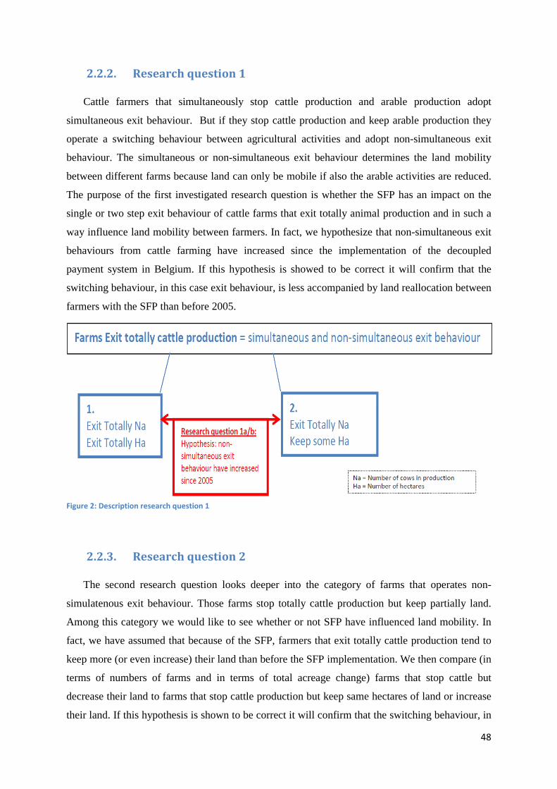
48

2.2.2. Research question 1

Cattle farmers that simultaneously stop cattle production and arable production adopt

simultaneous exit behaviour. But if they stop cattle production and keep arable production they

operate a switching behaviour between agricultural activities and adopt non-simultaneous exit

behaviour. The simultaneous or non-simultaneous exit behaviour determines the land mobility

between different farms because land can only be mobile if also the arable activities are reduced.

The purpose of the first investigated research question is whether the SFP has an impact on the

single or two step exit behaviour of cattle farms that exit totally animal production and in such a

way influence land mobility between farmers. In fact, we hypothesize that non-simultaneous exit

behaviours from cattle farming have increased since the implementation of the decoupled

payment system in Belgium. If this hypothesis is showed to be correct it will confirm that the

switching behaviour, in this case exit behaviour, is less accompanied by land reallocation between

farmers with the SFP than before 2005.

Figure 2: Description research question 1


The second research question looks deeper into the category of farms that operates non-

simulatenous exit behaviour. Those farms stop totally cattle production but keep partially land.

Among this category we would like to see whether or not SFP have influenced land mobility. In

fact, we have assumed that because of the SFP, farmers that exit totally cattle production tend to

keep more (or even increase) their land than before the SFP implementation. We then compare (in

terms of numbers of farms and in terms of total acreage change) farms that stop cattle but

decrease their land to farms that stop cattle production but keep same hectares of land or increase

their land. If this hypothesis is shown to be correct it will confirm that the switching behaviour, in

49

this case non simultaneous exit behaviour, is less accompanied by land reallocation between

farmers with SFP than before 2005 because those farms tend to keep more land in production.



To look at all the switching behaviour that could have been influenced by the SFP we have to

take into account partial switching behaviour, in other word farmers that partially exit cattle

production but not totally and that keep also producing land. Farms that stop partially cattle but

that stop totally land cannot (in principle) exist.

Among this category we would like to see whether or not the SFP have decreased land

mobility. In fact, we assumed that because of the SFP, farmers that exit partially cattle production

tend to keep more (or even increase) their land than before SFP. We thus compare (in terms of

numbers of farms and in terms of total acreage change concerned) farms that stop partially cattle

but decrease their land to farm that stop partially animal production but keep same hectares of

land or increase their land. If this hypothesis is shown to be correct it will confirm that partial

switching behaviour is less accompanied by land reallocation between farmers with SFP than

before 2005 because those farms tend to keep more land in production. Among this category of

farms we can construct our investigated research question with different degrees of change in

cattle production. We can than compare if farms that decrease more their degree of cattle

production tend to decrease more their land due to SFP than farms that decrease less their degree

of cattle production our inversely.

50



The fourth research question compiles farms that decrease totally (non-simultaneous exit

behaviour) and partially cattle production (partial switching behaviour) and that keep some land in

production. It adds research question 2 and research question 3 and it indicates if in total the SFP

tend to decrease more land reallocation. We thus compare in total farms that stop partially and

totally cattle but decrease their land to farm that stop partially and totally animal production but

keep the same hectares of land or increase their land. If we can prove that those farms tend to

decrease less their land than before the SFP implementation, it proves that land mobility has

decrease for farmers switching behaviour between agricultural activities with SFP.

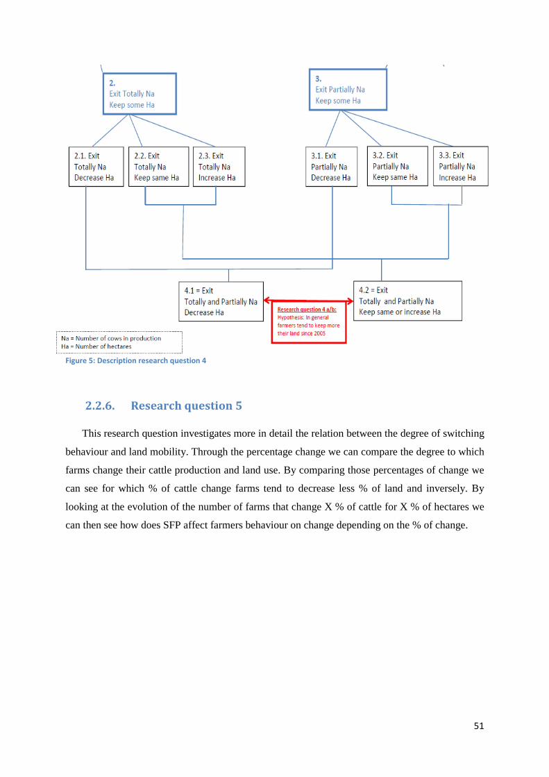
51



This research question investigates more in detail the relation between the degree of switching

behaviour and land mobility. Through the percentage change we can compare the degree to which

farms change their cattle production and land use. By comparing those percentages of change we

can see for which % of cattle change farms tend to decrease less % of land and inversely. By

looking at the evolution of the number of farms that change X % of cattle for X % of hectares we

can then see how does SFP affect farmers behaviour on change depending on the % of change.

52

3. Potential consequences of hypothesis

If our hypothesis seems to be true, that switching behaviour is less accompanied by land

mobility with decoupled payments, we could then prove that the SFP has decreased land mobility

between farmers in Belgium. Thanks to other impacts of decoupled payments explained below,

and identified in Belgium (Swinnen and al., 2008) i.e. barrier to exit and barrier to entry, we can

define that SFP in Belgium has decrease land mobility. Our postulate and the one that the SFP

creates a barrier to exit can explain the presence of more part time farming and more retired

farmers still in activities in Belgium.

If we can find significant results that support our postulate, we can conclude that the SFP

decreasing land mobility had a negative impact on the structural change in Flanders. In

contradiction to the positive structural change impact form increasing switching behaviour with

SFP, the decreasing land mobility that goes hand in hand with this switching behaviour influence

negatively structural change in Flanders by limiting land availability.

In the agricultural sector, there is a constant need for adjustment because competition

tends to stimulate larger and more efficient farms. Any policy that reduces asset mobility

decreases economic efficiency of agriculture. This could be the case for decoupled support by

reducing land mobility; Single Farm Payments could then be proved to contribute to a farm sector

that is less efficient than as it would have been otherwise. With limiting land mobility the ability

of producers to utilize land in their most productive way is constrained. On a first time this limited

mobility further contributes to higher average cost of production in the agriculture sector. On a

longer term the reducing asset mobility can increase the economic cost of future reforms. In fact,

because of limiting possible change to alternative economic activities and because of the

capitalization of current support into asset values, existing asset owners have interests in it and

may therefore resist future policy reform. It blocks especially future reforms reducing direct

payments because that would have negative consequences for new farmers. Recently, new

generations of farmers have invested in agriculture with the expectation that support in agriculture

would continue and they have paid a high entry cost. This is one of the reasons why for the EU

commission it’s difficult to engage in policy reforms that reduces support to the agricultural

sector. In compensation, EU has introduced the second pillar of the CAP, a policy designed to

promote structural adjustments. Rural development policy assists the setting-up of young farmers,

encourage the transition to more modern production practices or to more multifunctionnality in

agriculture.

By reducing land mobility, the SFP can slow down the restructuration of agricultural

sector and have indirect impact on efficiency of agricultural products. If our hypothesis is

53

confirmed, it gives then additional distorted effect on production and trade printing this thesis in

the debate explains below in the literature review.

If our hypothesis is correct it could answer a question raised by Kazukauskas and al. from

a study about productivity using Irish, Danish and Dutch farm level data. They prove that

decoupling policy has contributed to productivity growth. They find that farm enterprise

specialization had significant positive effects on farm productivity but that the switching

behaviour cannot explain the increase in productivity due to decoupled payments (Kazukauskas

and al., 2009). If we can assume that switching behaviour is partially accompanied by decreasing

land mobility, we can then understand that switching behaviour cannot explain the increase in

productivity.

54

C.Results

1. Global indicator measures

1.1. The total ratio of change per year

The “totalratiochange” indicates the total ratio change per year between changes in Ha for one

year compared with the change in number of cows (in livestock units) in production for one year.

The ratio has been calculated by dividing the change in acreage by the change in the cattle

number. The result show an increase of “totalratiochange indicating an increase in the ratio over

time (from 2003 to 2008), which contradicts the postulated hypothesis. The change in acreage per

farm seems to relatively increase compared to change in number of animals. However for the year

2005 the ratio has decreased compared to 2003 and 2004. So in 2005, the year of the SFP

implementation, land mobility has tended to decrease relatively compared to changes in cattle

production.

Table 1: The total ratio change per year of change in acreage on change in livestock units

totalratioofchange_graph

0.20.180.160.140.120.10.080.060.040.020

2003

2004

2005

2006

2007

2008

2003

2004

2005

2006

2007

2008

Gams instructions: ratiochangeovertime (ficnr, year) $ (changeNa(ficnr,year)ne 0)= (changeHa(ficnr,year)/changeNa(ficnr,year)); totalratioofchange (year)$ (number_farms(year)ne 0) = sum ((ficnr), (ratiochangeovertime (ficnr, year)))/number_farms(year)

55

1.2. The total ratio of percentage change per year

The total ratio of percentage change is a similar global indicator as the total ratio change but it

takes into account the degree of change in animal or hectares. By comparing percentage change in

Ha to percentage change in number cows from one year to another we can see if the percentage

change in acreage tends to decrease after 2005.

The results show a decrease for the year 2005 and 2006 relatively compared to year 2004, but

the year 2004 shows an increase compared to year 2003. For the years 2005 and 2006 we can

clearly notify a decrease in land mobility compared to the year 2004. But this is not true if we

compare those data to the year 2003. However in 2007 there is a high increase in land mobility

relatively compared to change in cattle production. In 2008 we have a negative decrease in land

mobility.

Table 2: The total ratio of percentage change per year of percentage change in acreage on percentage change in number

of cows

Those two indicators are global indicators because it takes into account exit, increase or

decrease in Ha or in cattle prodution. The difference in results for both indicators is relevant so it

seems important to look more in details at origins of those switching behaviour and their relation

with land mobility. To really answer our hypothesis, stating that switching behaviour increase by

SFP isn’t accompanied by mobile land, we have to focus on farms switching partially or totally

from cattle production.

totalratiopourcentagechange_graph

8006004002000-200-400-600-800-1,000

2003

2004

2005

2006

2007

2008

2003

2004

2005

2006

2007

2008

Gams instructions: PourcentagechangeHa(ficnr,year)$(animalnumber(ficnr,year)ne0) = (ChangeHa(ficnr,year)/animalnumber(ficnr,year))*100; PourcentagechangeNa(ficnr,year)$(totalsurface(ficnr,year) ne 0) = (ChangeNa(ficnr,year)/ totalsurface(ficnr,year))*100; ratioofpourcentagechange(ficnr,year)$(PourcentagechangeNa(ficnr,year) ne 0) = (PourcentagechangeHa(ficnr,year)/PourcentagechangeNa(ficnr,year)) *100 ;

56

2. Further investigation research questions

2.1. Research question 1

2.1.1. Research question 1A: In terms of total farm number

Let’s first define some indicators analyzed in absolute term. According to our data, the

number of farm that exit totally cattle production, including non-simultaneous exit behaviour and

simultaneous exit behaviour, has increased significantly from 515 farms in 2003 to 1352 farms in

2008.

Table 3 : The total number of farms per year that have exit totally cattle production

Among those farms the number of farms that adopt simultaneous exit behaviour has also

increased over time but it shows a huge increase from 76 farms in 2007 to 569 farms in 2008.

Until 2007, simultaneous exit behaviour corresponds to only 4 to 8% of the number of farms that

stop totally cattle production. It corresponds to a small percentage of the total exiting behaviour

and has a small influence on the global indicator measure (total ratio change). However this

percentage increases in 2008 to 42% of farms that exit animal production. So, we can already

notify that the importance of simultaneous exit behaviour has increased in the global ratio

measure for the year 2008.

Table 4 : The total number of farms per year that have adopted simultaneous exit behaviour

Farms that adopt non-simultaneous exit behaviour have also increased over time but it

presents a decrease in 2008. This increasing non-simultaneous exit behaviour could show

numberfarmexitNa

2003 2004 2005 2006 2007 2008

1,300

1,200

1,100

1,000

900

800

700

600

numberfarmexitNaandHa1

2003 2004 2005 2006 2007 2008

550

500

450

400

350

300

250

200

150

100

50

57

decreasing land mobility in Flanders but in order to interpret correctly those data, they have to be

analyzed in relative terms. In fact, the switching behaviour in general has increased over time and

it doesn’t reflect how this switching behaviour has been accompanied or not by mobile land.

Table 5: The total number of farms per year that have adopted non-simultaneous exit behaviour

By comparing in relative term the number of farm that exit totally cattle production and

crop production (simultaneous exit behaviour ) to farm that exit totally cattle production but keep

crop production (non-simultaneous exit behaviour), we obtain the following ratio ‘rapport1’.

Result shows that the ratio has increased over time. More precisely, simultaneous exit behaviour

relatively compared to non-simultaneous exit behaviour has tended to decrease slowly in 2005,

and then increase slowly after 2005 and significantly in 2008. Except for the year 2005, it

contradicts our hypothesis that non-simultaneous exit behaviour tends to increase in comparison

to simultaneous exit behaviour. So it seems that the SFP has not negatively affected the link

between exiting behaviour and the land mobility.

Table 6: The ratio of the number of farms that adopt simultaneous exit behaviour on the number of farms that adopt

non-simultaneous exit behaviour

numberfarmexitNaandkeepHa

2003 2004 2005 2006 2007 2008

820800780760740720700680660640620600580560540520

rapport1a

2003 2004 2005 2006 2007 2008

80

70

60

50

40

30

20

10

0

20032004 2005

2006

2007

2008

58

2.1.2. Research question 1B: In terms of total acreage change

When we look at the total acreage change per year for farms that exit totally cattle

production and keeping some land, it seems that total change in acreage (mobile land) from these

farms has increased since 2005 (details in annex 2). However, it can only be interpreted by

comparing with the total quantity of mobile land per year from farms with simultaneous exit

behaviour. This ratio has been calculated under ‘rapport 1b’. Rapport 1b indicates the ratio of total

acreage change of farms stopping totally cattle production and crop production to farms stopping

totally cattle production and keeping some Ha. This ratio corresponds to the share of mobile land

due to simultaneous exit behaviour relatively compared to the share of mobile land due to non-

simultaneous exit behaviour.

Table 7 : The ratio of total acreage change per year of farms that adopt simultaneous exit behaviour on the total acreage

change for farms that adopt non-simultaneous exit behaviour

Because it corresponds to both decreasing land mobility changes, this indicator cannot

prove if land mobility has increased or not, but it shows from which type of switching behaviour

was mobile land predominant.

The ratio shows an increase in 2005, a decrease in 2006-2007 and an increase in 2008. In

2005 compared to 2003-2004, the share of mobile land from simultaneous farm exit behaviour has

increased relatively compared to the share of mobile land from non-simultaneously exit

behaviour. In 2006-2007, the share of mobile land from non-simultaneous farm exit has increased

relatively compared to the share of mobile land from simultaneously exit behaviour. But in 2008,

the share of mobile land from simultaneous farm exit behaviour has raised consequently

compared to the share of mobile land from non-simultaneously exit behaviour. It means that for

the years just after the 2003 Cap reform implementation (2006-2007), land mobility in terms of

acreage change has tend to be more important from farms exiting totally animal production and

keeping crop production than from farmers exiting totally both farming activities. But in 2005 and

Rapport1b

2003 2004 2005 2006 2007 2008

1,400

1,200

1,000

800

600

400

200

0

20032004

2005

2006 2007

2008

Gams instructions:

Rapport1b(year) $ (TotalchangeHAforfarmsexitNAandkeepHA(year)ne 0) = ((TotalchangeHAforfarmsexitNAandHA(year))/ TotalchangeHAforfarmsexitNAandkeepHA(year))*100 ;

59

2008 the share of mobile land was more significant from famers that exit totally both farming

activities.

2.1.3. Research question 1: Conclusion

In conclusion we can state that non-simultaneous exit behaviour do not tend to increase in

comparison to simultaneous exit behaviour since the SFP implementation. So farms that exit

totally cattle production do not tend to keep more their land since 2006.

We can however remark that in 2005 the number of farms applying non-simultaneous exit

behaviour has tended to be a bit more preponderant than simultaneous exit behaviour. And for

2005 the share of mobile land from simultaneous exit behaviour among mobile land has increased

compared to 2003-2004. So it shows that farms have tended to keep more land and more farms

have applied non-simultaneous exit behaviour decreasing land mobility during the year of the SFP

implementation.

We can also remark the huge increase in land mobility for the year 2008. This increase

comes from the huge increase in simultaneous exit behaviour in 2008. Simultaneous exit

behaviour is a small share of farm exiting totally animal production but this share has been

increased in 2008 (42%). Simultaneous exit behaviour has a bigger influence in 2008 on land

mobility. That can also explain the higher share of mobile land coming from simultaneous exit

behaviour notice in the ratio ‘rapport 1b’.

2.1.4. Critics

For this indicator we compare more reliable data to less reliable data. In fact, from our

data, simultaneous exit behaviour could be biased because small changes in farms structure and

population could be registered as simultaneous exit behaviour. The dataset could contain changes

in the farm identifier key because of several reasons: farms that are taking over by a successor

don’t keep same identification number as the preceding owner, farms switching location but

keeping same owner (move from one building to another), creation of group or association of

farmers into one farm, administrative change in numbers characterizing farms (fincr). So we could

consider that data over simultaneous exit behaviour are not so reliable in our dataset. Next

analysis will allow us to look at land mobility without taking into account data over simultaneous

exit behaviour.

Another remark is based on simple supposition concerns the structure of farmer’s

population. In fact, a higher share of farmer’s population becomes closest to the age of retirement,

and these farmers adopt then simultaneous exit behaviour. Land mobility could be positively

influence by the number of farmers going into retirement and this could interfere with impact of

60

SFP on land mobility. In order to avoid this bias from farmer age structure we can look at land

mobility impact from farmers adopting a non-simultaneous behaviour and a partial switching

behaviour.

61



Among farms that adopt non-simultaneous exit behaviour we can differentiate farms that

have decreased their land, increased their land or keep the same acreage after an exit of cattle

production. By comparing the two panel period in absolute terms, it seems that the number of

farms that keep some Ha but that decrease land tend to increase until 2007 then decrease in 2008.

The numbers of farms that keep some Ha but that increase or keep the same acreage tend to

increase from 2005 to 2006 then it decreases in 2007 and 2008.

Table 8 : The number of farms per year that adopt non-simultaneous exit behaviour and that decrease acreage

Table 9: The number of farms per year that adopt non-simultaneous exit behaviour and that increase or keep same

acreage

To compare the change in crop production in relative terms, we have calculated the ratio

of the number of farms that exit totally cattle production and decrease their crop production to the

number of farms that exit totally cattle production and increase or keep the same acreage in

production. The purpose is to look if farms change their acreage differently after stopping animal

production with the implementation of the SFP. If farmers decrease less Ha than before 2005

relatively compared to farms that keep same Ha or increase Ha when they stop animal production,

it decreases land mobility.

numberfarmexitNaandkeepsameHaandincrease

2003 2004 2005 2006 2007 2008

360

340

320

300

280

260

240

220

numberfarmexitNaandkeepHadecrease

2003 2004 2005 2006 2007 2008

480460440420400380360340320300280260240

62

The result shows a decreasing ratio for this category of switching behaviour from 2003 to

2006. But the ratio increases in 2007-2008 so it contradicts our hypothesis for this two years

period. In 2006, we find more farmers increasing their Ha among farmers adopting non-

simultaneous exit behaviour compared to 2004 and 2005. In 2007-2008, we find more farmers

decreasing their Ha among farmers adopting non-simultaneous exit behaviour than before. So for

the years 2007 and 2008 land mobility has increased from farmers adopting non simultaneous

behaviour.

Table 10: Among non-simultaneous exit behaviour farms, the ratio of the number of farms that decrease their acreage on

the number of farms that increase or keep the same acreage


The total acreage change from farms that have exit totally cattle production and have

increased their crop production is positive and vary over time but the total acreage change for

farms that have exit totally cattle production and have decreased their crop production is negative

and has increased over time except for 2008 (detailed results in annex 3).

In order to compare both situations, over decreasing or increasing crop production, we

have calculated the ratio ‘rapport2b’ of total acreage change for farm exit cattle production and

decreasing crop production on total acreage change for farm exit cattle production and increasing

crop production. The ratio shows a decrease in 2005 indicating a greater acreage change from

farms that increase their crop production relatively compared to farms that decrease their crop

production. However in 2006-2007-2008, this ratio increases so compared to 2005 total mobile

land from farmers that decrease their crop production increase. To conclude, it term of acreage

change, land mobility from non-simultaneous behaviour has decreased in 2005 but increased in

2006-2007-2008.

rapport2a

2003 2004 2005 2006 2007 2008

140

120

100

80

60

40

20

2003

20042005

2006

20072008

Gams instructions:

Rapport2a(year) $ (numberfarmexitNaandkeepsameHaandincrease (year) ne 0) = (numberfarmexitNaandkeepHadecrease(year)/ numberfarmexitNaandkeepsameHaandincrease (year))*100 ;

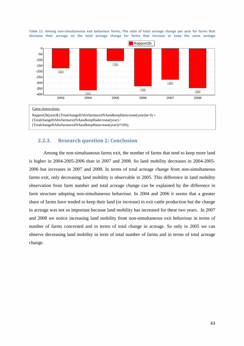
63

Table 11: Among non-simultaneous exit behaviour farms, The ratio of total acreage change per year for farms that

decrease their acreage on the total acreage change for farms that increase or keep the same acreage


Among the non-simultaneous farms exit, the number of farms that tend to keep more land

is higher in 2004-2005-2006 than in 2007 and 2008. So land mobility decreases in 2004-2005-

2006 but increases in 2007 and 2008. In terms of total acreage change from non-simultaneous

farms exit, only decreasing land mobility is observable in 2005. This difference in land mobility

observation from farm number and total acreage change can be explained by the difference in

farm structure adopting non-simultaneous behaviour. In 2004 and 2006 it seems that a greater

share of farms have tended to keep their land (or increase) in exit cattle production but the change

in acreage was not so important because land mobility has increased for these two years. In 2007

and 2008 we notice increasing land mobility from non-simultaneous exit behaviour in terms of

number of farms concerned and in terms of total change in acreage. So only in 2005 we can

observe decreasing land mobility in term of total number of farms and in terms of total acreage

change.

Rapport2b

2003 2004 2005 2006 2007 2008

0

-50

-100

-150

-200

-250

-300

-350

-400

2003

2004

2005

2006

2007

2008

Gams instructions:

Rapport2b(year)$ (TotalchangeHAforfarmsexitNAandkeepHaincrease(year)ne 0) = (TotalchangeHAforfarmsexitNAandkeepHadecrease(year) / (TotalchangeHAforfarmsexitNAandkeepHaincrease(year))*100);

64


Farms that adopt a partial switching behaviour are farms that exit partially cattle production

but not totally. Among these farms and in parallel to the change in cattle production, we can

differentiate farms that decrease their land, increase their land or keep the same land after a partial

switch from cattle production. We can also differentiate among partial switching behaviour farms,

different degree of change in switching cattle production. We have then analyzed this category

using different references in cattle switching behaviour with minus 5, 10, 20, 30 or 50 Livestock

Unit cows from one year to another. Results are presented more in details in annex 4. In order to

summarize we will look at farmers that have decreased their cattle production by more than 10

cows in one year.


In absolute terms, we notice that for (almost) each degree of switching behaviour the

number of farms that tend to decrease their crop production in reducing cattle production has

increased until 2007 and then decreased in 2008. In reverse the numbers of farms that tend to

increase Ha or keep same Ha in reducing cattle production has increased until 2008. This

difference occurs for each degree of switching behaviour always for the year 2008.

Table 12 : The evolution of the number of farms that decrease cows in production by more than 10 livestock units and

that decrease their crop production

Table 13: The evolution of the number of farms that decrease cows in production by more than 10 livestock units and

that increase or keep the same acreage in production

numberfarmchangeNa2andHadecrease

2003 2004 2005 2006 2007 2008

500

450

400

350

300

250

200

numberfarmchangeNa2keepsameHaandincrease

2003 2004 2005 2006 2007 2008

320

300

280

260

240

220

200

180

65

To understand better what are trend behind it; let’s first look at the change in total cattle

number.

Table 14: The evolution of the number of cows in production

Cattle sector has known a restructuration in 2007-2008. In fact, from our data, total cattle

in production increase in 2007 and then decrease in 2008. In 2007, the number of farms that

decreases their cattle production by more than 5% has increased and the number of farms that

increases their cattle production by more than 5% has also increased. However in 2008, the

number of farms that increases their cattle production by more than 5% has decreased and the

number of farms that decreases their cattle production by more than 5% has increased.

Table 15: The evolution of the number of farms that decrease their cattle production by more than 5% but that stay on

cattle production.

Table 16: The evolution of the number of farms that increase their cattle production by more than 5%.

totalanimalnumber

2002 2003 2004 2005 2006 2007 2008

440,000

430,000

420,000

410,000

400,000

390,000

380,000

numberfarmchangeNa_5andkeepHa

2003 2004 2005 2006 2007 2008

6,000

5,500

5,000

4,500

numberfarmchangeNa5andkeepHa

2003 2004 2005 2006 2007 2008

4,8004,6004,4004,2004,0003,8003,6003,4003,200

66

In order to compare the number of farms that change in crop production, increase or keep

same acreage compared to decrease in acreage, we have calculated the ratio ‘rapport 3a’ between

the number of farms switching partially cattle production and decreasing Ha onto the number of

farms switching partially cattle production and increasing or keeping same quantity of acreage.

The result points out a decreasing ratio for the year 2005 and 2006 showing a decreasing

mobility of land associated with partial switching behaviour. Also the year 2008 can be

interpreted as a decreasing land mobility compared to the year 2007 but it depends on degree of

change and on the years before we compare to it. In 2005, 2006 and 2008, a part of farms that exit

partially cattle production have kept more land or increase their land relatively compared to the

part of farmers that have decreased their land in production. This decreasing mobility is not

observable anymore in 2007; it shows an increasing mobility of land from partial switching

behaviour farmers.

For the year 2008, the greater number of farms inducing decreasing land mobility is more

observed from farms with higher degree of change in cattle production.

For farms decreasing by more than 35 Unit Livestock cows per year, the predominance of

farms decreasing mobility of land after 2005 is not perceptible anymore; such farms demonstrate

even an increase in land mobility. So it seems that the quantity of animals changed is important

and it could be interesting to look deeper into degree of change of cows and Ha. This will be

further discussed in research question 5.

Table 17: The ratio of the number of farms that decrease their acreage on the number of farms that keep the same or

increase their acreage for farms decreasing by more than 10 livestock units their cattle production

rapport3a2

2003 2004 2005 2006 2007 2008

180

160

140

120

100

80

60

40

20

0

20032004

2005 2006

2007

2008

Gams instructions:

rapport3a2(year)$(numberfarmchangeNa2keepsameHaandincrease(year) ne 0 )=

((numberfarmchangeNa2andHadecrease(year)/numberfarmchangeNa2keepsameHaandincrease(year))*100);

(TotalchangeHAforfarmsexitNAandkeepHaincrease(year))*100);

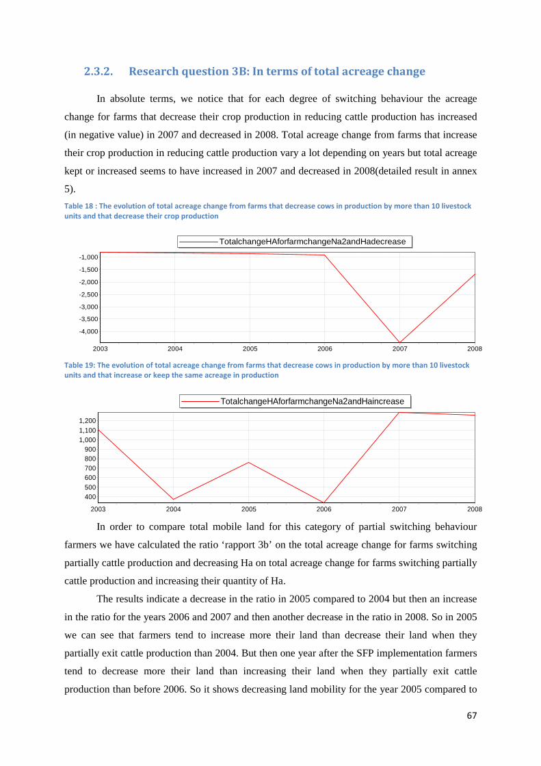
67


In absolute terms, we notice that for each degree of switching behaviour the acreage

change for farms that decrease their crop production in reducing cattle production has increased

(in negative value) in 2007 and decreased in 2008. Total acreage change from farms that increase

their crop production in reducing cattle production vary a lot depending on years but total acreage

kept or increased seems to have increased in 2007 and decreased in 2008(detailed result in annex

5).

Table 18 : The evolution of total acreage change from farms that decrease cows in production by more than 10 livestock

units and that decrease their crop production

Table 19: The evolution of total acreage change from farms that decrease cows in production by more than 10 livestock

units and that increase or keep the same acreage in production

In order to compare total mobile land for this category of partial switching behaviour

farmers we have calculated the ratio ‘rapport 3b’ on the total acreage change for farms switching

partially cattle production and decreasing Ha on total acreage change for farms switching partially

cattle production and increasing their quantity of Ha.

The results indicate a decrease in the ratio in 2005 compared to 2004 but then an increase

in the ratio for the years 2006 and 2007 and then another decrease in the ratio in 2008. So in 2005

we can see that farmers tend to increase more their land than decrease their land when they

partially exit cattle production than 2004. But then one year after the SFP implementation farmers

tend to decrease more their land than increasing their land when they partially exit cattle

production than before 2006. So it shows decreasing land mobility for the year 2005 compared to

TotalchangeHAforfarmchangeNa2andHadecrease

2003 2004 2005 2006 2007 2008

-1,000

-1,500

-2,000

-2,500

-3,000

-3,500

-4,000

TotalchangeHAforfarmchangeNa2andHaincrease

2003 2004 2005 2006 2007 2008

1,2001,1001,000

900800700600500400

68

2004. But the year 2004 shows increasing land mobility compared to 2003. And the year 2006 to

2007 shows increasing land mobility compared to the years preceding the SFP implementation. In

2008 however we face new decreasing land mobility; farmers tend to decrease less their land. So

for the year 2005 and 2008 results confirm our hypothesis, land mobility decrease in term of total

acreage change from partial switching behaviour. But for the year 2006 and 2007 results

contradict our hypothesis, land mobility increases in term of total acreage change from partial

switching behaviour.

For the category of farmers that have decreased their cattle production by more than 40

cows per year, it seems that we observe decreasing mobility of land for the year 2007 and 2004. It

allows us to illustrate that for higher change in cow number, farmer behaviour is different.

Table 20: The ratio of the total acreage change of farms that decrease their acreage on the total acreage change from

farms that keep the same or increase their acreage

2.3.3. Research question 3: conclusion

When we look at partial switching behaviour (partial exit cattle production and keep some

hectares), it seems that in 2005, 2006 and 2008 number of farms that tend to keep their land has

increased compared to year before the SFP implementation and so it tends to decrease land

mobility. But in 2007 it’s not the case anymore. In taking into account total acreage change, it

seems that only for the year 2005 and 2008 decreasing land mobility from partial switching

behaviour can be observed. But this decreasing land mobility is relative to the year 2004 that

shows increasing land mobility compared to 2003. Indisputably we notice a huge increase in land

mobility in 2007 from number of farm and from total acreage change concerned. For the year

2006 we notice increasing mobility of land in term of number of farms that tends to keep less land

but this is not so observable in term of total number of acreage change.

rapport3b2

2003 2004 2005 2006 2007 2008

0

-50

-100

-150

-200

-250

-300

-350

2003

2004

2005

2006

2007

2008

Gams instructions:

rapport3b2(year)$(TotalchangeHAforfarmchangeNa2andHaincrease(year)ne 0) = ((TotalchangeHAforfarmchangeNa2andHadecrease(year)/TotalchangeHAforfarmchangeNa2andHaincrease(year))*100);

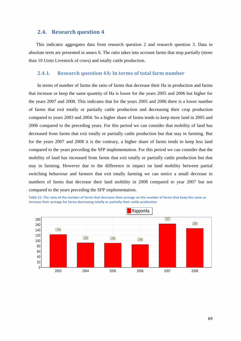
69


This indicator aggregates data from research question 2 and research question 3. Data in

absolute term are presented in annex 6. The ratio takes into account farms that stop partially (more

than 10 Units Livestock of cows) and totally cattle production.


In terms of number of farms the ratio of farms that decrease their Ha in production and farms

that increase or keep the same quantity of Ha is lower for the years 2005 and 2006 but higher for

the years 2007 and 2008. This indicates that for the years 2005 and 2006 there is a lower number

of farms that exit totally or partially cattle production and decreasing their crop production

compared to years 2003 and 2004. So a higher share of farms tends to keep more land in 2005 and

2006 compared to the preceding years. For this period we can consider that mobility of land has

decreased from farms that exit totally or partially cattle production but that stay in farming. But

for the years 2007 and 2008 it is the contrary, a higher share of farms tends to keep less land

compared to the years preceding the SFP implementation. For this period we can consider that the

mobility of land has increased from farms that exit totally or partially cattle production but that

stay in farming. However due to the difference in impact on land mobility between partial

switching behaviour and farmers that exit totally farming we can notice a small decrease in

numbers of farms that decrease their land mobility in 2008 compared to year 2007 but not

compared to the years preceding the SFP implementation.


increase their acreage for farms decreasing totally or partially their cattle production

Rapport4a

2003 2004 2005 2006 2007 2008

180160140120100

80604020

0

2003

2004 20052006

2007

2008

70


In terms of total acreage change, we have calculated the ratio ‘rapport 4 b’ between the

total acreage change from farms decreasing their acreage in production and the total acreage

change from farms increasing or keeping same quantity of Ha. It shows that this ratio is lower in

2005 compared to 2004. But then in 2006 and 2007 this ratio increases compared to the years

before the SFP implementation. In 2008, the ratio decreases compared to the years 2004, 2006 and

2007 but it doesn’t decrease compared to 2003. So it seems that, in terms of total acreage change,

land mobility from partial switching behaviour and non-simultaneous exit behaviour has

decreased significantly in 2005 and less significantly in 2008 compared to 2004. In 2006, 2007

land mobility in terms of total acreage change has increased from partial switching behaviour and

non-simultaneous exit behaviour compared to the years before the SFP implementation.


farms that keep the same or increase Ha in production


From farms that exit totally and partially cattle production and keep some hectares of land

we can conclude that land mobility has decreased only for the years 2005 and 2008. This proves

to be the case in terms of the number of farms that tend to keep more land and in terms of total

acreage change from farms concerned. But in terms of total acreage change, land mobility has

decreased compared to the year 2004 but not compared to the year 2003. The years 2003 and

2004, are ambiguous to interpret because the Fischler reform was already announced so farmers

could have adapted their behaviour in prevision of the reform. In this case, we face a problem of

lack of data to confirm that our hypothesis is true for the years 2005 and 2008.

However for the years 2006-2007 we can conclude that there is increasing land mobility.

For the year 2006 it has to be discussed because on one hand the number of farms that tend to

keep more land has increased. On the other hand total acreage change induced by these farmers is

not significant to show decreasing land mobility compared to the years before the SFP

Rapport4b

2003 2004 2005 2006 2007 2008

0

-50

-100

-150

-200

-250

-300

-350

2003

2004

2005

2006

2007

2008

71

implementation. This single result over number of farms is not relevant to confirm our hypothesis

for the year 2006.

This aggregate indicator looks at land mobility for partial switching behaviour and for

non-simultaneous behaviour. If we add to it the land mobility impact from simultaneous exit

behaviour (from research question1), we have a complete overview on the relation between

switching behaviour due to SFP (exit and decreasing animal production) and mobile land. The

decomposition process gives us nuances on impact for each type of switching behaviour.

2.4.4. Critics

The way indicators from research question 2 and research question 3 have been calculated

can be emphasized.

Firstly, we separate farmer’s behaviour whether if they decrease or increase acreage

compared to the years preceding the SFP implementation. But even a small increase or decrease in

Ha is sufficient to categorize it in one category or another. So it doesn’t reflect if farmer’s

behaviour is a strategy for the long term or if it reflects occasional circumstances.

And secondly, in terms of total acreage change our calculation doesn’t allow us to take

into account farmers that keep the same acreage as the year before. Our indicators over total

acreage change compare acreage change from farms increasing their Ha to acreage change from

farms decreasing their Ha. So results over number of farms permit to see better if farmers tend to

keep exactly same acreage as the year before than results over total acreage change.

72


This last research question develops two investigations using percentage change in cattle

production and acreage. We focus on farmers that switch partially cattle production to develop

further results from research question 3. The first investigation looks at number of farms for

which land mobility decrease or increase according to different percentage changes in cattle

production. The second investigation calculates the average percentage change in acreage for

each category of percentage changes in animal production.

2.5.1. Research question 5: Investigation over difference in

percentage change.

Within this fifth research question we would like to see how SFP have influenced land

mobility from partial switching behaviour according to different degree of percentage change in

cattle number. One possible way is to look at the number of farms that has changed “X” percent in

their animal production from one year to another. According to their change in percentage change

in acreage we compare farmers that decrease less or decrease more their percentage change in

acreage than their percentage change in cattle production.

Does a decrease in cattle production by “X” % have induced a decrease by more than

“X”% or by less than “X”% of Ha in production? To look among degree of change we analyze

this question in using different decrease in percentage change of animals in production by more

than 5%, more than 10%, more than 20%, more than 30% and more than 50%. Let’s explain in

details results for one of the category analyzed. The results over different categories are explained

in annex 7.

The first graph indicates the number of farm that decreases number of cattle by more than

-5 % and that in the same time decrease acreage by less than – 5%. Farms that decrease acreage

by less than -5% have increased in 2008.

Table 23 : Among farms that decrease the number of cows by more than -5 %, the number of farm per year that decrease

acreage by less than -5%

Nbrfarm_decreaselessHathanchangeNa_5

2003 2004 2005 2006 2007 2008

5,000

4,800

4,600

4,400

4,200

4,000

3,800

3,600

3,400

73

Second graph indicates the number of farm that decrease number of animals by more than

-5 % and that in the same time decrease acreage by more than -5%. Farms that decrease acreage

by more than -5% have increased in 2007 and decreased in 2008.


acreage by more than -5%

Total land mobility increasing or decreasing has to be relatively compared to see how SFP

have impacted on this relation. So we have compared for each degree of change the difference

between both numbers of farms, it’s the ratio of number of farms. The following ratio

‘rationumbersfarm_5’ corresponds to the number of farms that decrease acreage by more than –

5% under number of farm that decrease acreage by less than – 5% for farms that decrease number

of animals by more than -5 %.

If the ratio increases it shows that the number of farms that tend to decrease by more than

X% their land when they switch X % of cattle production increase. If the ratio decreases it shows

that the number of farms that tend to decrease by less than X% their land when they switch X %

of cattle production increase. An increasing ratio shows that farmers tend to decrease more in

percentage their acrerage than their animal number; it increases land mobility. So the decreasing

ratio shows that farmers tend to decrease less in percentage their acreage than their animal

number, it decreases land mobility.

Table 25 : The ratio corresponds to the number of farm that decrease acreage by more than -5% under number of farm

that decrease acreage by less than - 5% for farm that decrease number of animals by more than -5%

Nbrfarm_decreasesameHathanchangeNa_5

2003 2004 2005 2006 2007 2008

1,500

1,400

1,300

1,200

1,100

1,000

900

800

700

rationumber_farms5

2003 2004 2005 2006 2007 2008

0.45

0.4

0.35

0.3

0.25

0.2

0.15

0.1

0.05

0

2003 2004

2005

2006

2007

2008

74

For each percentage of change we can see almost the same trend that occurs. The indicator

is quite similar to the indicator from the research question 3 looking at partial switching

behaviour, except that this new one takes into account percentage change acreage and animal

number. Results are then quite similar. We will not develop in details the results for each cattle

percentage change; they are presented in annex 8.

Compared to our preceding results from research question 3, this indicator confirms that

we face a higher number of farms that tends to keep their land in 2005, 2006 and 2008. In 2005,

2006 and 2008 it can be showed that the number of farms that tend to decrease less their

percentage change of acreage than their percentage change of cattle in production has increased

relatively compared to the number of farms that tend to decrease their acreage change by the same

percentage than percentage change in animals. We can conclude that investigation over different

degree of percentage change in cattle production (presented in annex 8) does not demonstrate

significant difference depending on degree of percentage change.

Results present above, illustrating a decrease by more than 5% of cattle production,

enclose each farm that decrease by more than 5% their cattle production. We assume that a

decrease of 5% in animal production should demonstrate farmers’ motivation to decrease cattle in

production in a long term perspective. This is a difference with research question 3. In fact, in

Units Livestock in production we cannot define a value that can objectively demonstrate a long

term switching behaviour of farmers due to variability in size of farms.

This investigation looks at difference in terms of percentage change in animal number

however it doesn’t look at difference between category of cattle change, it takes cumulative

changes (Higher than -5%, higher than -10%, higher than – 20%, higher than -50). To see if small

percentage changes in animal production have more impact on land mobility than higher

percentage change in animal production, we can divide the analysis of percentage change in

different categories of percentage change.

Gams instructions:

Nbrfarm_decreaselessHathanchangeNa_5(year) = Sum ((ficnr),(PourcentagechangeHa(ficnr,year)>-5)

$(PourcentagechangeNa(ficnr,year)<-5)$(animalnumber(ficnr,year)>0));

Nbrfarm_decreasesameHathanchangeNa_5(year) = Sum ((ficnr),(PourcentagechangeHa(ficnr,year)<-5)

$(PourcentagechangeNa(ficnr,year)<-5)$(animalnumber(ficnr,year)>0)) ;

rationumber_farms5(year)$ (Nbrfarm_decreaselessHathanchangeNa_5(year) ne0) =

Nbrfarm_decreasesameHathanchangeNa_5(year)/Nbrfarm_decreaselessHathanchangeNa_5(year) ;

75

2.5.2. Research question 5: Investigation over average percentage

change

One additional analysis is the calculation of average percentage change in land for each

category of percentage change in animal production. Through this indicator we can address quantity

of acreage change in average for farms that switch partially cattle production.

Firstly we calculate the average percentage change in acreage for all farms switching partially

cattle production. It’s the global average percentage in Ha for each change in cattle production. The

average percentage change that goes with any decrease in cattle production is –4 % of Ha in 2005, -

4.6% of Ha in 2006 and -3.3% of Ha in 2008. For these three years, 2005, 2006 and 2008, the

average percentage change in Ha decreases less than in 2004. Compared to 2004, it shows a decrease

in land mobility, because farmers tend to decrease less in average their percentage acreage change.

But compared to 2003, it doesn’t show a decrease in land mobility because the average percentage

change in Ha in 2003 is really low (-1.07%).

Table 26 : The average percentage change in acreage for all farms switching partially cattle production

Secondly we have analyzed the average percentage change in acreage for different

categories of average percentage change in cattle production. The different categories investigated

are the following:

- Average percentage change in cattle production from -5 to –10%






Average_percentage_changeHachangeNa

0-1-2-3-4-5-6-7-8-9-10-11-12-13

2003

2004

2005

2006

2007

2008

2003

2004

2005

2006

2007

2008

Gams instructions:

Average_percentage_changeHachangeNa (year) $ (number_farmstot(year) ne 0) =

Sum ((ficnr) $ ((PourcentagechangeNa(ficnr,year)<0) and (animalnumber(ficnr,year)>0)),

PourcentagechangeHa(ficnr,year))/number_farmstot(year);

76

The results for each category are presented more in details in annex 9 and some

conclusions are presented in the following paragraph.

When we look at a high level of average percentage change in cattle, we cannot clearly

show a coherent trend because results vary a lot according to different categories of cattle

percentage change. The year 2003 has been a year with low decrease in acreage average

percentage change in comparison to percentage change in number of animals. The year 2007

clearly shows a high increase in land mobility for each category except for the last one, category

with average percentage in Na from -80 to -60. It seems that year 2008 has known more

decreasing land mobility with small percentage of change in animal production (average

percentage change in Na from –10 to -5, from -20 to -10, from – 5 to 0) than with high percentage

change in animal production (average percentage change in Na from -50 to –30).

77

3. Interpretation of results

1

Land Mobility

Farm number Farm number Total Ha Change Farm number Total Ha Change Farm number Total Ha Change

2004 / Decrease Increase / Increase Decrease Increase

2005 Decrease Decrease Decrease Decrease Decrease Decrease Decrease

2006 Small Increase Decrease Increase Decrease Increase Decrease Increase

2007 Small Increase Increase Increase Increase Increase Increase Increase

2008 Huge increase Increase Increase Decrease Decrease Increase Decrease

Ass

um

pti

on

s

Simultaneous farm

exit behaviour has

decreased reletively

compare to non-

simultaneous farm

exit behaviour

2005 True

2006 False

2007 False

2008 False

2 3 4Research

question: Land Mobility Land Mobility Land Mobility

False

True

False

False

True

True

False

False

True

Among non-simultaneous

farms exit, farms tend to eep

more land and do not tend to

decrease more land when

they exit cattle production

Among partial switching

behaviour farms tend to

keep more land and do not

tend to decrease more their

land when they exit partially

cattle production

Among non-simultaneous

farms exit and partial

switching behaviour farms

tend to keep more land but

do not tend to decrease

more their land.

True

False

False

78

In conclusion we can say that switching behaviour induced by SFP is accompanied by

mobile land and SFP don’t decrease land mobility. Only in 2005 increasing switching behaviour

seems not to be supplemented by mobile land and decreasing land mobility can be observed in

2005 compared to years before the SFP implementation. We can conclude that there is a trend

toward decreasing land mobility in 2005 because for each indicator we find decreasing land

mobility in terms of total acreage change and in terms of number of farms. In 2005, we have

observed increasing non-simultaneous exit behaviour compared to simultaneous exit behaviour.

Among non-simultaneous exit behaviour we find more farmers that tend to keep or increase their

land relatively compared to farmers that tend to decrease their land compared to the years 2003

and 2004. The third category of partial switching farmers, also shows decreasing land mobility in

2005. In fact, compared to the years 2003 and 2004, this category of farms tends to keep or

increase their land relatively compared to farmers that tend to decrease their land in exiting cattle

production. But we cannot clearly determine that this decreasing land mobility is a consequence

of the SFP implementation.

In fact, to confirm that this decreasing land mobility in 2005 is due to the SFP

implementation, it would have be more reliable to look also at data before 2003, i.e before the

announcement of the form the 2003 CAP reform was going to take place. From 2003 to 2005,

some farmers could have already adapted their behaviour in trying to gather more land for

example. That’s maybe a reason why we can find increasing mobility of land in 2004 compared to

2003 for some indicators. Some farmers could have also delayed their switching behaviour in

2003 or 2004 to switch from cattle production after the SFP implementation. The huge variability

in results between the year 2003 and the year 2004 hinder us to conclude in an affirmative way

that SFP have decreased land mobility in 2005.

For the year 2006, we can find an increasing number of farms that tend to keep or increase

their land when they exit totally or partially cattle production. However, the impact on land

mobility is not relevant because in terms of total acreage change, there is increasing land mobility

in 2006 compared to the years before the SFP implementation. Three reasons could be exposed to

explain this difference. Firstly farmers keeping or increasing their land can have a smaller

structure compared to farms that were decreasing their land when exit partially or totally cattle

production in the same period, so it concerns less Ha. But this reason cannot be supported by

results from research question 5 over percentage change in animal production. Secondly, farms

keeping or increasing their land when they exit totally or partially cattle production tend to keep

their land but in lower quantity than in 2005. The indicator over average percentage change

(research question 5) shows that the average percentage change in acreage when farms switch

partially from cattle production is higher in 2006 than in 2005. Thirdly among results over the

79

number of farms, the majority of farms classified as farms that tend to keep or increase their Ha in

2005 are farms that tend to keep exactly the same acreage as year before. And farmers keeping

exactly same Ha are not observable in the indicator over total acreage change but this reason is

less probable.

The increase in land mobility can be uncontestably observed in 2007. In fact, for each

type of switching behaviour observed we find increasing land mobility in 2007.

In 2008 depending on the type of switching behaviour results are different.

In 2008 we notice an increase in land mobility due to the huge increase in simultaneous

exit behaviour relatively compared to non-simultaneous behaviour. But from farms with partial

switching behaviour decreasing land mobility is observed in 2008 in terms of farm number and

total acreage change. The research question 4, aggregating farms with non-simultaneous

behaviour and partial switching behaviour, shows also decreasing land mobility for the year 2008.

The global indicator (total ratio of change) doesn’t show decreasing land mobility for the year

2008. This is due to the fact that this global indicator takes also into account mobile land from

simultaneous exit behaviour. For the year 2008 due to its huge increase, simultaneous exit

behaviour had more weight in the global ratio than previous years, attenuating the decreasing land

mobility impact from farmers with non-simultaneous exit behaviour and partial switching

behaviour.

One unexpected result concerns the difference in land mobility between 2007 and 2008.

For both years an increase in switching behaviour can be commented: increase in partial switching

behaviour in 2007 and 2008 and increase in simultaneous exit behaviour in 2008.

In 2007 the total number of animals in production has increased, the number of farms that

increases their cattle production by more than 5% has increased and the number of farms that

decreases their cattle production by more than -5% has also increased. So, the increase in land

mobility can be partly combined to this increase in switching behaviour from both senses, from

the increase in cattle production or from the decrease in cattle production.

In 2008, the total numbers of cattle has decreased compared to 2007, the number of farms

that increases their cattle production by more than 5% has decreased and the number of farms that

has decreased their cattle production by more than 5% has increased.

For the year 2007 and 2008 we find more switching behaviour because more farms

decrease their cattle production. However a difference in land mobility exists because in 2007

switching behaviour were supplemented by mobile land and in 2008 switching behaviour in cattle

production were less accompanied by mobile land. We suggest in the following paragraph that

this difference in the relation between switching behaviour and land mobility could be explained

by differences in the origin of farmers switching behaviour.

80

In 2007 we assume that the switching behaviour comes from a restructuration of the cattle

sector because some farms have decreased their animal production, and others have increased

their animal production in 2007. In 2008, more farms have decreased their animal production but

fewer farms have increased their animal production. So it seems that economic purpose was less

positive in 2008 than 2007. The high share of farms that have adopted a simultaneous behaviour

in 2008 also confirms this assumption; it can be due to bankruptcy in farming or by retired/aged

farmers that stop more early their activities due to bad economic situation.

When we compare our results to reality of political reforms and prices in agricultural

products, we can maybe explain part of results with the dairy sector crisis. In fact, the milk price

has firstly known a huge increase in 2007-2008, after a long period of milk price stabilization,

then in 2008-2009 the milk price has known a huge decrease stimulating more farmers to stop

their production. The increase in animal production in 2007 could maybe be explained by the high

milk price in 2007. Farmers could have tended to increase their animal production but it doesn’t

explain why farms that decreased animal production were accompanied by land mobility. In 2008

the increasing land mobility coming from the raise in simultaneous exit behaviour could be

interpreted as an impact of dairy sector crisis on farms bankruptcy. But the end of the year 2008

was only the beginning of this dairy crisis price so it seems quite early to observe already the

consequences in the data. However in 2008, farmers that switch partially cattle production could

be a consequence of low milk price, farmers have tended to decrease more their animal production

because of the bad economic conjuncture. Those partial switching farmers were not in long term

strategy to exit farming. That could be a potential reason to explain why farmers switching

partially cattle production have kept more land in 2008, showing decreasing land mobility for

some indicators in 2008.

The Health Check, the Mid-term review of CAP agreed in November 2008 could have had

a potential impact on land mobility but also this could not yet be measured through this database.

81

4. Suggestions

In this last chapter we develop some suggestions based on problems that we had to face

with data use or research question purpose.

4.1. Problems with data analysis

Data over farms that exit totally cattle production and crop production cannot be considered

as reliable as other values from our dataset. In fact, some farms changing status are interpreted as

farms that stop totally both production but in reality it could be the cases of farms that enter an

association, farms take over by a successor... Furthermore in 2008 we note a high increase for

farms stopping animal production and crop production. From 76 farms adopting simultaneous exit

behaviour (exit animal in production and crop production) in 2007 to 569 farms in 2008. We have

checked it and this share of farms that exit totally farming corresponds more or less to a trend

toward increase in number of farms exiting farming. In 2007, 1288 farms have exit totally farming

and in 2008 28918 farms have exit totally farming according to yearly national agricultural

census.

Total number of farms in Flanders 2003 2004 2005 2006 2007 2008 2009

With agricultural production

36577 35486 34410 33272 31984 30666 29394

Source : http://statbel.fgov.be/nl

To overpass this potential bias in data we have looked also at land mobility from farmers

adopting non-simultaneous exit behaviour and partial switching behaviour because for those

farms we don’t face same problem relate to farms registration.

A second problem that we had to face with data is the lack of data before 2002, to

understand better how mobile land accompanied by switching behaviour has evolved, it would

have been better to compare data after 2005 to data before 2003. In our data we cannot say if

behaviour in 2003 and 2004 has been distorted by the CAP reform announcement and difference

in the results between the year 2003 and 2004 are mostly significant.

The third problem is related to the fact that in our database information before 2006 didn’t

make a distinction between suckler cows and dairy cows. Further investigation should use data

that differentiate dairy cows in production from sucker cows in production. Impacts of SFP on

both productions aren’t similar. Suckler cows still benefits from direct subsidies (suckler cow

82

premium) linked to production, so the decoupling effect isn’t similar for suckler cows than for

dairy cows. If we could have differentiated both types of cows we could have analyzed more

what have been the consequences on land mobility of decoupling for dairy cows. Trends in the

market and in politics aren’t the same for both types of livestock. If we could have differentiated

dairy cows from suckler cows we could have concluded if a decrease or an increase in both output

and input prices interferes in the relation between switching behaviour and land mobility.

Lastly we can address an issue related to our data reliability. In fact, from our database we

note a huge increase in total number of cows in production in 2007 but in data from national

agricultural Census, a similar trend is not observable. According to information from the national

agricultural Census, the total numbers of cows in Flanders decrease continuously since 2003 and

from 2005 to 2007, the number of suckler cows has increased and then decreased in 2008. In our

database the decrease in total number of cows in production in 2008 corresponds. But the increase

in total number of cows in production in 2007 doesn’t fit. A possible reason explaining this

difference could be due to the specificity of our data. Data comes from ‘mestbank’ administration

and in 2007 the manure action plan changed in Flanders. Changed in the way farmers fill in

different category during data collection can be the cause of this difference.

Numbers of cows in Flanders

2003 2004 2005 2006 2007 2008 2009

Cows 529.595 522.053 513.623 506.295 504.273 494.907 500.414

Milk cow 328.630 319.743 308.883 300.081 294.319 289.738 296.951

Suckler cows 200.965 202.310 204.740 206.214 209.954 205.169 203.463 Source: http://lv.vlaanderen.be/nlapps/docs/default.asp?id=904

4.2. Potential effects that could have increased land mobility

As we have concluded, except for the year 2005, switching behaviour due to SFP is

accompanied by mobile land and so land mobility has increased since 2006. We can identify some

factors that could have influenced positively land mobility interfering in the relation between

switching behaviour from SFP and land mobility.

- The age of farmer population.

Old farmers coming into retirement and stopping production bring high share of land into land

market. Some retired farmers keep their land but this seems to be smaller than the share of farmers

stopping totally agricultural production. A possible trend that we can see in countryside is that

some old farmers keep some animals in small quantity, so they switch partially production and

83

decrease their land also partially. This has happened since ages but the high share of old farmers

in the active farmer’s population is high nowadays and so it can have an important influence in

statistic.

- 2003 2004 2005 2006 2007 2008

Number of farmers older than 50 18.878 18.354 17.977 17.496 17.012 16.411 with potential succesor 2.563 2.511 2.459 2.323 2.338 2.215 without potential succesor 11.904 11.341 11.125 10.721 10.215 9.510 Don't know 4.411 4.502 4.393 4.452 4.459 4.686

Source : http://lv.vlaanderen.be/nlapps/docs/default.asp?id=904

- The economic conjoncture.

As we could maybe interpret from difference in results between the years 2007 and 2008,

the change in competitiveness of the sector is important. Agricultural sector competitiveness

concerns price of outputs (milk for dairy cow or meat for suckler cows) and prices of inputs. Both

interfere a lot with the switching behaviour and its relation with land mobility. In fact, if prices are

bad and if inputs costs are high, some farmers could tend to reduce their production because of the

high cost of entrants. This reduction in animal production will not be accompanied by mobile

land, because this trend is temporary. On the other side with bad price, farmers could also increase

their production in order to compensate for the lack of income. If price are good farmers tend to

decrease less their animal production. There is certainly an interaction in the relation of switching

behaviour and mobile land with economic conjuncture. But throughout this thesis we cannot

interpret the way this interaction takes. Further analysis could also look at this link. With data

after 2009 (after end of milk crisis) in parallel to data distinguishing dairy cows to suckler cows

we could better interpret impact of economic conjuncture on the relation of switching behaviour

and mobile land.

- Suckler cow premium

Decoupling effect has it has been implemented in 2005, is not totally coupled for suckler

cows because there is a suckler cow premium that has been implemented in Flanders since 2005.

Farmers who have suckler cows on their farms and that are used for rearing calves for meat

production can request the suckler cow premium. This suckler cow’s premium concerned 6357

farms in Flanders in 2008. A farmer has a defining number of suckler cow premium rights; it’s the

suckler cow quota. The premium corresponds to maximum 250€ per animal, the total support has

decreased over year for the purpose of modulation for the CAP second pillar. This premium still

encourages farmers to keep on with suckler cow’s production so it distorts the decoupling effect

84

of SFP. Our analysis over the decoupling effect on land mobility in enclosing suckler cows has

been a bit biased because there are still some coupled effects from suckler cow premium.

Suckler cow premium 2005 2006 2007 2008

Numbers of farms concerned 7179 6908 6612 6357

Total support in € 30129764 29870602 29564193 29493054

Average support per farm 4197 4324 4471 4639 Source : http://lv.vlaanderen.be/nlapps/docs/default.asp?id=904

- Dairy quota

For dairy cow production, direct payments are well decoupled from production since 2005.

But there are still quota systems that represent some values for farmers because they had to pay to

gather the right to produce their quota. We can maybe assume that this quota still produce coupled

effect to milk production inducing less switching behaviour from milk production. Quota mobility

regulation play also an important role over the switching behaviour of farmers from dairy cows

production. If quota mobility regulations are too binding farmers will switch less easily from dairy

production. This dairy quota also limits increase in milk production. By limiting milk production,

land demand is also limited because the total number of cattle production on a farm is limited by

the soil connection legislation.

- The manure legislation

Since 1991, Flanders has implemented a manure legislation limiting farmers in their animal

production expansion without land in order to respect a European Directive. This manure policy

permits to guarantee a better water and ground quality in order to realize the objectives of the

Nitrates directive and over ammonia reduction. In 2007 entirely new manure legislation has been

reformulated. According to the manure decree, farmers are required to process a portion of their

manure surplus. The new legislation calculated this manure limitation per farm in a different way

and now it’s partly based on local production pressure from animal manure and special attention

is paid to dairy cows because the nutrient excretion is made proportional to the milk productivity.

The new manure legislation has strengthened the weight of manure legislation on farmer

production behaviour. This manure reform in combination with good price of milk and meat in

2007 could have increased pressure on land demand to compensate for the change in manure

limitation per cows. From our data analysis we have notice that in 2007 farmers switching from

cattle production has tended to decrease more their acreage. This increasing land mobility find in

our results could maybe be partly explained by this new manure legislation in 2007 stimulating

land demand for some farmers (without switching behaviour).

85

Conclusion

To conclude we can say that our hypothesis cannot be confirmed. Switching behaviour

after the SFP implementation has been accompanied by mobile land. This means that the SFP did

not affect negatively land mobility. The way we have decompose the analysis in different type of

switching behaviour has allowed us to have a broad overview over switching behaviour due to the

SFP implementation and over their relation with land mobility. Firstly, the exit behaviour of

farmers from cattle production has been analyzed and we cannot prove, in contrast as we had

predicted, increasing non simultaneous behaviour over simultaneous exit behaviour after the SFP

implementation. Among non-simultaneous exit behaviour we can also not prove that farmers tend

to keep more land after the SFP implementation. Then the partial switching behaviour of farmers

from cattle production has been analyzed, among those farms we cannot prove that they tend to

keep more their land than before the SFP implementation.

Even if for some years some results can be argued in favor of decreasing land mobility,

the decreasing land mobility impact from SFP cannot be clearly derived from our results. In fact,

the observed change in the different calculated ratios do not seem to be related with changes in the

SFP policies. Apparently other factors have stronger effects on land mobility than SFP. In our last

chapter we propose some potential other factors that can have interacted in this relation of SFP

switching behaviour and mobile land. Economic circumstances seem to have played an important

role and some coupled effect such dairy quota mobility regulation, suckler cow premium… have

stronger influence on land mobility than the change in SFP.

We were assuming that the decreasing land mobility that could go hand in hand with this

switching behaviour could influence negatively structural change in Flanders by limiting land

availability. But with this conclusion over our results we cannot induce of a negative impact on

the structural change from SFP implementation in Flanders. If SFP have a positive impact on land

mobility, it could mean that SFP entitlement right market works and that this market is not so

constrained as could have observed Swinnen and al. (2008). On one hand increasing switching

behaviour accompanied by mobile land due to SFP doesn’t reinforce the problem induced by rigid

rental market in Belgium that is to constrain restructuring of agricultural sector. On the other hand

the capitalization effect of SFP can reinforce the problem induced by rigid rental market but we

didn’t analyze the capitalization effect of SFP in land rents. To have a better view on the impact

of SFP on the restructuration process of agricultural sector, the interaction of land capitalization

effect and land mobility effect from SFP change should then be investigated.

86

ListofReferences

• Adams, G., Westhoff, P., Willott B. and. Young II R.E. (2001). Do decoupled payments

affect US crop area? Preliminary evidence from 1997 to 2000, American Journal of Agricultural Economics 83 (5), p. 1190–1195.

• Antón, J. (2009). What role for Policy in Agricultural Risk Managemen? , AES-DEFRA Conference on Coping with Risk in UK Agriculture, 22 January 2009, London.

• Alston, J.M. and. James J.S. (2002) The Incidence of Agricultural Policy. In: Gardner B. L. and Rausser G. C. (éd.), Handbook of Agricultural Economics, Vol. 2B, p. 1689-1749.

• Alston, J. M. (2007). Benefits and Beneficiaries from U.S. Farm Subsidies, AEI Agricultural Policy Series: The 2007 Farm Bill and Beyond. American Enterprise Institute.

• Bhaskar A., John C. Beghin. (2009). How coupled are decoupled farm payments? A review of the evidence. Journal of agricultural and resource economics 34(1) 130-153

• Bartolini, F., Latruffe L., Viaggi, D. (2011). Assessing the effect of the CAP on farm innovation adoption. An analysis in two French regions, Paper prepared for the 122nd EAAE Seminar, February 17-18, 2011, Ancona, Italy

• Bartolini F., Viaggi D., Ronchi D., Gomez y Paloma S. and Sammeth F. (2011). Assessing the impact of future CAP reforms on the demand of production factors, Paper prepared for the 122nd EAAE Seminar, February 17-18, 2011, Ancona, Italy

• Bartolini F., Viaggi D., Floridi M. (2010). Assessment of present trends, mechanisms and impact of the CAP on structural change and innovation, CAP_IRE, CAP_IRE report.

• Bougherara D., Latruffe L. (2010). Potential impact of the EU 2003 CAP reform on land idling decisions of French landowners: Results from a survey of intentions, Land Use Policy 27, p. 1153–1159

• Breen, J.P., Hennessy, T.C., Thorne, F.S., (2005). The effect of decoupling on the decision to produce: an Irish case study. Food Policy 30 (2), p. 129–144.

• Bureau, J.C., Mahé, L.P. (2008). CAP reform beyond 2013: An idea for a longer view, Notre Europe Report, Paris

• Calus, M., Vandermeulen V., Rogge E., Emde L., Dessein J., Lauwers L.& Van Huylenbroeck G. (2010).Wijkers en blijvers in de Vlaamse land- en tuinbouw, Beleidsdomein Landbouw en Visserij, afdeling Monitoring en Studie, Brussel.

• Ciaian, P., Swinnen J.F.M. (2009). Credit market imperfections and the distribution of policy rents, American Journal of Agricultural Economics 91 (4), p. 1124-1139.

• Ciaian, P. and Swinnen J.F.M (2006). Land Market Imperfections and Agricultural Policy Impacts in the New EU member states: A Partial Equilibrium Analysis, American Journal of Agricultural Economics, 88(4), p. 799-815.

• Ciaian, P. and Swinnen J.F.M. (2007). Credit Market Imperfections and the Distribution of Policy Rents: The Common Agricultural Policy in the New EU member states, LICOS Discussion Paper 183/2007, LICOS, University of Leuven.

• Ciaian, P., Kancs D. and Swinnen J.F.M. (2008). Static and Dynamic Distributional Effects of Decoupled Payments: Single Farm Payments in the European Union, LICOS Discussion Paper 207/2008, LICOS, University of Leuven.

• Clancy, D., Kazukauskas, A., Newman, C., Thorne, F. (2009). An investigation of the level of structural change in the agrifood sector of Ireland, Denmark and the Netherlands, The Rural Economy Research Centre Working Paper Series, Teagasc

87

• Coyle, B. (2005). Dynamic econometric models of Manitoba crop investment and production under risk aversion and uncertainty. Working paper, OECD, Paris.

• Duvivier, D., Gaspart F. and de Frahan B.H. (2005). A Panel Data Analysis of the Determinants of Farmland Price: An Application to the Effects of the 1992 CAP Reform in Belgium, Paper presented at the 11th EAAE Congress, 23-27 August, 2005, Copenhagen.

• Féménia F., Gohin A. and Carpentier A. (2008). The decoupling of farm programs: Revisiting the wealth effect, paper presented at 108st EAAE Seminar, 8-9 February, 2008, Warsaw, Poland.

• Gallerani, V., Gomez y Paloma, S., Raggi, M., Viaggi, D. (2008). Investment behaviour in conventional and emerging farming systems under different policy scenarios. JRC Scientific and Technical Reports, Institute for Prospective Technological Studies (IPTS), Seville.

• Guyomard, H., Le Mouël C. and Gohin A. (2004). Impacts of alternative agricultural income support schemes on multiple policy goals, European Review of Agricultural Economics, 31(2), p. 125-148.

• Goodwin, B. K. and. Mishra A. K. (2006). Are “Decoupled” Farm Program Payments Really Decoupled? An Empirical Evaluation, American Journal of Agricultural Economics 88, p. 73-89.

• Goodwin, B.K., Mishra A.K and Ortalo-Magné F.N. (2003). What’s Wrong with Our Models of Agricultural Land value?, American Journal of Agricultural Economics, 85, p. 744-752.

• Hennessy, T. (2004a). An analysis of the impact of decoupling using Irish FADN data. FAPRI-Ireland Partnership, Rural Economy Research Centre, Teagasc, Athenry, Ireland.

• Hennessy, T. (2004b) Projecting farm numbers, Paper Prepared for 2015 AgriVision Committee, Appendix 4 2015 AgriVision Report, Irish Department of Agriculture and Food.

• Hennessy, T., Rehman, T. (2006). Modelling the impact of decoupling on structural change in the farming sector: integrating econometric and optimization models. Rural Economy Working Paper Series, Teagasc, Athenry, Ireland.

• Hennessy, T, Thorne, F.S. (2005). How decoupled are decoupled payments? The evidence from Ireland. Eurochoices, 4, p. 30-35.

• Hennessy, D. (1998). Production Effects of Income Support under Uncertainty. American Journal of Agricultural Economics 80, February 1998, p. 46-57.

• Howley, P., Donnellan, T., Hanrahan, K., (2011). An Analysis of the Potential Impact of Decoupled Payments: An Irish Case, EuroChoices, Avril 2011, Vol. 10, p. 26-30

• Howley, P., Hanrahan, K. et al. (2009) The 2003 CAP Reform: Do Decoupled Payments Affect Agricultural Production?, RERC Working papers, Teagasc.

• IRES-UCL (2004). La Politique Agricole Commune, Regards Economiques 19, Louvain-La-Neuve

• Jambor A., Harvey D. (2010). Cap Reform Options: a challenge for analysis and synthesis, Paper presented at the AES Annual Conference, March 29 – 31, 2010, Edinburgh.

• Janssen, S.J.C., van Ittersum, M.K. (2007). Assessing farm innovations and responses to policies: A review of bio-economic farm models, Agricultural Systems 94, 2, p. 622-636

• Kallas Z., Serra T. and Gil J.M. (2009). Effects of policy instruments on farm investments and production decisions in the Spanish cop sector, Paper presented at the 113th EAAE Seminar, September 3 - 6, Chania, Crete, Greece.

• Kazukauskas, A., Newman, C. and Thorne, F. (2009). Decoupling policy effect and Irish dairy farms productivity estimation using Olley/Pakes. Trinity College Dublin.

88

• Kazukausas A., Newman C. (2010). Cap reform and its impact on structural change and productivity growth: a cross country analysis, Paper presented at the 114th EAAE Seminar, April 15 – 16 , Berlin, Germany.

• Kazukausas A., Newman C and Sauer J. (2011). CAP Reform and Its Impact on Structural Change and Productivity Growth: A Cross Country Analysis, TEP Working Paper, No. 0411 February 2011.

• Key, N. and Roberts, M.J. (2009). Nonpecuniary benefits to farming: Implications for supply response to decoupled payments to decoupled payments. American Journal of agricultural Economics, 91(1), p. 1-18.

• Lecture reader AEP 20306: Dr.ir. C Gardebroek, Dr.ir. J.H.M. Peerlings, (2010) Economics of Agribusiness, Agricultural Economics and Rural Policy Group, Wageningen University

• OECD (2001). Decoupling: a conceptual overview, OECD Papers No. 10, OECD, Paris. • OECD (2004). Analysis of the 2003 CAP Reform, OECD, Paris.

• OECD (2007). Agricultural support, farm land values and sectoral adjustment; the implications for policy reform, AGR/CA/APM(2006)19/final, Paris.

• Patton M., Kostov P., McErlean S, Moss J. (2008). Assessing the influence of direct payments on the rental value of agricultural land, Food Policy 33, p. 397–405

• Piet L., Desjeux Y., Latruffe L. and Le Mouël C. (2010). How do agricultural policies influence farmland concentration? The example of France, Paper presented at the 114th EAAE Seminar, April 15 - 16, Berlin, Germany.

• Ritson C. (éd.), Harvey (1997). The common agricultural policy, CAB International, Royaume-Uni. 440 p.

• Roberts, M.J., Key N. (2008). Agricultural payments and land concentration: A semiparametric spatial regression analysis, American Journal of Agricultural Economics 90 (3), p. 627-643.

• Roberts, M.J., Kirwan, B., Hopkins, J. (2003). The incidence of government program payments on agricultural land rents: the challenges of identification, American Journal of Agricultural Economics 85 (3), p. 762–769.

• SCENAR 2020 (2006). Scenario Study on Agriculture and the Rural World, European Commission, Directorate-General Agriculture and Rural Development, Brussels.

• Sckokai, P. (2005). Modelling the impact of agricultural policies on farm investments under uncertainty: the case of the CAP arable crop regime. Working paper, AGR/CA/APM(2005)13/FINAL, Paris, OECD.

• Sckokai, P. and. Moro. D (2006). Modeling the Reforms of the Common Agricultural Policy for Arable Crops under Uncertainty, American Journal of Agricultural Economics 88(1), p. 43–56.

• Serra, T., Zilberman D., Goodwin B. K., and Featherstone A. M. (2005a). Decoupling Farm Policies: How Does this Affect Production?, Paper presented at the American Agricultural Economics Association Annual Meeting, July 24-27, 2005, Providence, Rhode Island,

• Serra, T., Zilberman, D., Goodwin, B.K. and Featherstone, A.M. (2006). Effects of decoupling on the mean and variability of output, European Review of Agricultural Economics, Vol. 33(3), p. 269-288

• Swinnen, J.F.M. (2009). On the Future of Direct Payments. Paper presented at the BEPA Workshop. February 26, 2009, European Commission, Brussels

• Swinnen, J.F.M., Ciaian P. and Kancs d’A. (2008). Study on the Functioning of Land Markets in the EU Member States under the Influence of Measures Applied under the Common Agricultural Policy, Final Report, Centre for European Policy Studies (CEPS), Brussels

89

• Swinnen J., van der Zee F. A, (1993). The Political Economy of Agricultural Policies : A Survey, European Review of Agricultural Economics 20

• Viaggi D., Raggi M., Gomez y Paloma S. (2009). Facing decoupling: use of payments and investment reaction to decoupling in the EU, Paper presented at the International Association of Agricultural, Economists Conference, August 16-22, 2009, Beijing, China.

• Vrolijk, H.C.J., de Bont C.J.A.M, Blokland P. W. and Soboh R.A.M.E. (2010). Farm viability in the European Union; Assessment of the impact of changes in farm payments, LEI ,LEI Report 2010-011, The Hague

• Westcott, P. C. and Young E.C. (2002). Influences of Decoupled Farm Programs on Agricultural Production, Paper presented at the Conference on Free Trade of the Americas, the WTO, and New Farm Legislation: Responding to Opportunities and Challenges, May 23-24, 2002, San Antonio, Texas.

• Zier P., Petrick M., (2010). CAP reform and the effects of direct payments on heterogeneous farm structures in East Germany, Gewizola.

• http://www.europarl.europa.eu/factsheets/4_1_1_en.htm

• http://www.wto.org/

• http://europa.eu/legislation_summaries/agriculture/general_framework/ag0003_en.htm

• http://europa.eu/legislation_summaries/agriculture/general_framework/l60002_en.htm

• http://www.vcm-mestverwerking.be

• http://lv.vlaanderen.be/nlapps/docs/default.asp?id=904

• http://statbel.fgov.be/nl

• http://lv.vlaanderen.be/nlapps/docs/default.asp?fid=5

• http://www.vlm.be/landtuinbouwers/mestbank/Pages/default.aspx

91

Appendices

Table of contents

Annex 1: Summary of the communication on "The CAP towards 2020" .............................................. 92

Annex 2: Research question 1B ............................................................................................................. 93

Annex 3: Research question 2 B ........................................................................................................... 94

Annex 4: Research question 3 A ............................................................................................................ 95

Annex 5: Research question 3 B ............................................................................................................ 99

Annex 6: Research question 4A ........................................................................................................... 103

Annex 7: Research question 4B ........................................................................................................... 104

Annex 8: Research question 5 - Investigation over difference in percentage change ........................ 105

Annex 9: Research question 5 - Investigation over average percentage change ............................... 110

92

Annex 1: Summary of the communication on "The CAP towards 2020"

In the following paragraph we highlight some relevant information published in the

Commission’s communication. The communication has revealed three main challenges for the

future CAP : food security, environment and climate change and territorial balance. The first

objective of the CAP would then to provide viable food production. In order to achieve this CAP

should continue to support to farm incomes mainly due to risk uncertainty in price (price

volatility) and in production (natural risks). Cap should also “improve the competitiveness of the

agricultural sector and to enhance its value share in the food chain”. In areas with specific natural

constraints CAP should compensate for production difficulties. The second objective for the

future CAP would provide sustainable management of natural resources and climate action. In

order to achieve this CAP should guarantee sustainable production practices and provision of

environmental public goods. It could be done by fostering green growth through innovation.

Mitigation and adaptation actions to pursue climate change should also be address. The third

objective of the future CAP is to pursue balanced territorial development by supporting rural

employment, promoting and by allowing structural diversity in farming systems. More

specifically to direct payments necessary adaptions have been mentioned in order to add value

and quality in spending of the CAP. Direct payments should be made more understandable to the

taxpayer and it should fulfill two functions: the basic income function, and the environmental

function to reward farmers for the provision of public goods. In future CAP concrete application

of decoupled payments will be redistribute, redesign and better targeting. Changes in the design of

direct payments should go hand in hand with a better definition and targeting of support to active

farmers. In order to improve the distribution of payments between farmers an upper ceiling for

direct payments should be introduced ("capping"). A “greening” component of direct payments

should be added by supporting actions addressing both climate and environment policy goals.

Those actions should go beyond cross-compliance and are linked to agriculture (e.g. permanent

pasture, green cover, crop rotation and ecological set-aside). An additional income support should

be provided to farmers in areas with specific natural constraints in the form of an area-based

payment. Markets measures should be maintained only as a safety net tool.

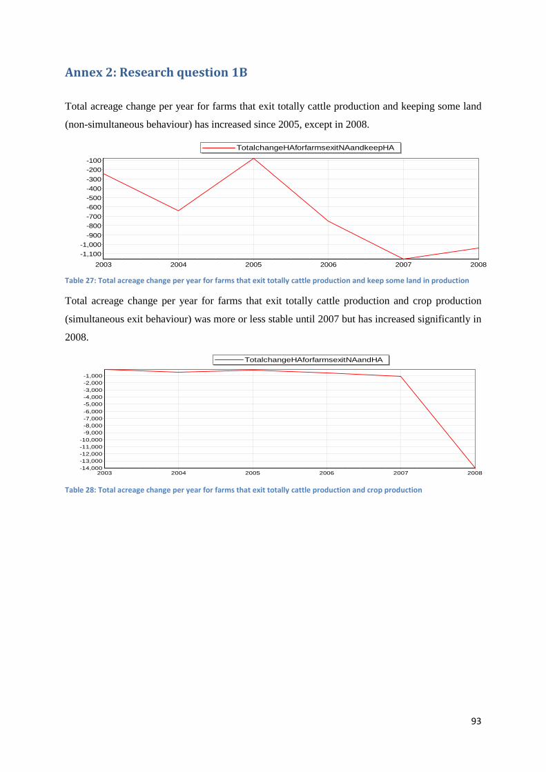
93

Annex 2: Research question 1B

Total acreage change per year for farms that exit totally cattle production and keeping some land

(non-simultaneous behaviour) has increased since 2005, except in 2008.

Table 27: Total acreage change per year for farms that exit totally cattle production and keep some land in production

Total acreage change per year for farms that exit totally cattle production and crop production

(simultaneous exit behaviour) was more or less stable until 2007 but has increased significantly in

2008.

Table 28: Total acreage change per year for farms that exit totally cattle production and crop production

TotalchangeHAforfarmsexitNAandkeepHA

2003 2004 2005 2006 2007 2008

-100

-200

-300

-400

-500

-600

-700

-800

-900

-1,000

-1,100

TotalchangeHAforfarmsexitNAandHA

2003 2004 2005 2006 2007 2008

-1,000-2,000-3,000-4,000-5,000-6,000-7,000-8,000-9,000

-10,000-11,000-12,000-13,000-14,000

94


Among farms that adopt non-simultaneous exit behaviour we can differentiate farms that have

decreased their land, increased their land or keep the same acreage after an exit of cattle

production. By comparing the two panel period in absolute terms, the total acreage change for

farms that have exit totally cattle production and have decreased their crop production is negative

and has increased over time except for 2008. On the other hand the total acreage change from

farms that have exit totally cattle production and have increased their crop production is positive

and vary over time.

Table 29 : Among farms adopting non-simultaneous behaviour, total acreage change per year for farms that keep or

increase their acreage

Table 30: Among farms adopting non-simultaneous behaviour, total acreage change per year for farms that decrease

their acreage

TotalchangeHAforfarmsexitNAandkeepHaincrease

2003 2004 2005 2006 2007 2008

750

700

650

600

550

500

450

400

350

300

250

TotalchangeHAforfarmsexitNAandkeepHadecrease

2003 2004 2005 2006 2007 2008

-600

-800

-1,000

-1,200

-1,400

-1,600

-1,800

95

Annex 4: Research question 3A

Among farms that adopt a partial switching behaviour (farms exit partially cattle production) we

can differentiate different degree of change in switching cattle production. The following

categories of degree of change in cattle production have been analyzed: decrease by 5, 10, 20, 35

Livestock Unit for cows in production. For each category of change in cattle production we can


switch from cattle production. Then we have calculated for each categories of change the ratio

between the number of farms switching partially cattle production and decreasing Ha on the

number of farms switching partially cattle production and increasing or keeping same quantity of

Ha.

Farms that decrease cows in production by more than 5 livestock units:

Table 31 : The evolution of number of farms that decrease cows in production by more than 5 livestock units and that

decrease their crop production

Table 32: The evolution of number of farms that decrease cows in production by more than 5 livestock units and that

increase or keep the same acreage in production




2003 2004 2005 2006 2007 2008

1,200

1,100

1,000

900

800

700

600


2003 2004 2005 2006 2007 2008

850

800

750

700

650

600

550

500

rapport3a1

2003 2004 2005 2006 2007 2008

160

140

120

100

80

60

40

20

0

2003 2004

2005

2006

2007

2008

96









2003 2004 2005 2006 2007 2008

500

450

400

350

300

250

200


2003 2004 2005 2006 2007 2008

320

300

280

260

240

220

200

180

rapport3a2

2003 2004 2005 2006 2007 2008

180

160

140

120

100

80

60

40

20

0

20032004

2005 2006

2007

2008

97









2003 2004 2005 2006 2007 2008

180

160

140

120

100

80

60

40


2003 2004 2005 2006 2007 2008

90

80

70

60

50

40

rapport3a3

2003 2004 2005 2006 2007 2008

220200180160140120100

80604020

0

20032004

2005

2006

2007

2008

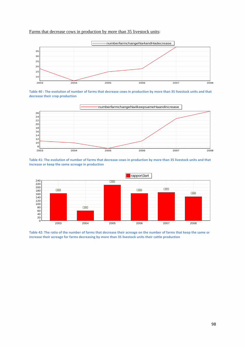
98









2003 2004 2005 2006 2007 2008

35

30

25

20

15

10


2003 2004 2005 2006 2007 2008

26

24

22

20

18

16

14

12

10

8

rapport3a4

2003 2004 2005 2006 2007 2008

240220200180160140120100

80604020

0

2003

2004

2005

20062007

2008

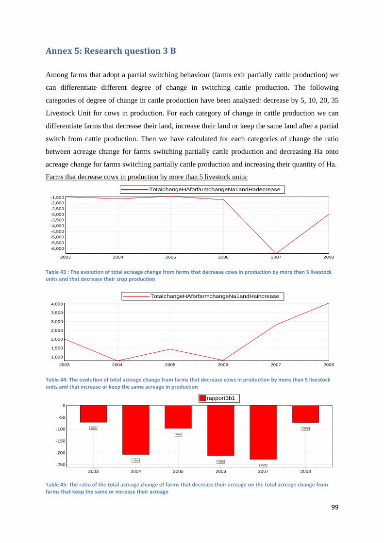
99

Annex 5: Research question 3 B

Among farms that adopt a partial switching behaviour (farms exit partially cattle production) we

can differentiate different degree of change in switching cattle production. The following

categories of degree of change in cattle production have been analyzed: decrease by 5, 10, 20, 35

Livestock Unit for cows in production. For each category of change in cattle production we can


switch from cattle production. Then we have calculated for each categories of change the ratio

between acreage change for farms switching partially cattle production and decreasing Ha onto

acreage change for farms switching partially cattle production and increasing their quantity of Ha.









2003 2004 2005 2006 2007 2008

-1,500-2,000-2,500-3,000-3,500-4,000-4,500-5,000-5,500-6,000


2003 2004 2005 2006 2007 2008

4,000

3,500

3,000

2,500

2,000

1,500

1,000

rapport3b1

2003 2004 2005 2006 2007 2008

0

-50

-100

-150

-200

-250

2003

2004

2005

2006

2007

2008

100












2003 2004 2005 2006 2007 2008

-1,000

-1,500

-2,000

-2,500

-3,000

-3,500

-4,000


2003 2004 2005 2006 2007 2008

1,2001,1001,000

900800700600500400

rapport3b2

2003 2004 2005 2006 2007 2008

0

-50

-100

-150

-200

-250

-300

-350

2003

2004

2005

2006

2007

2008


2003 2004 2005 2006 2007 2008

-400

-600

-800

-1,000

-1,200

-1,400

-1,600

-1,800

101











2003 2004 2005 2006 2007 2008

600550500450400350300250200150100

rapport3b3

2003 2004 2005 2006 2007 2008

0

-100

-200

-300

-400

-500

-600

-700

2003

2004

2005

2006

2007

2008


2003 2004 2005 2006 2007 2008

-50-100-150-200-250-300-350-400-450-500-550-600


2003 2004 2005 2006 2007 2008

350

300

250

200

150

100

50

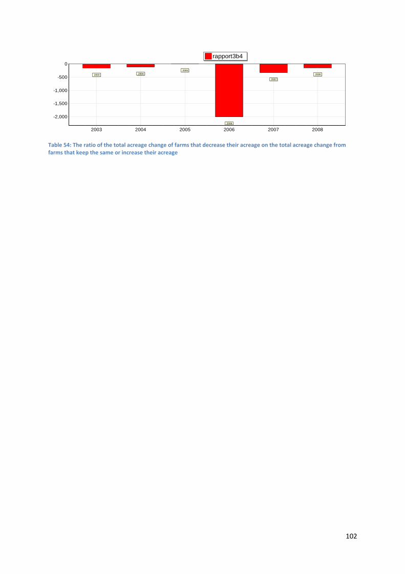
102



rapport3b4

2003 2004 2005 2006 2007 2008

0

-500

-1,000

-1,500

-2,000

2003 20042005

2006

2007

2008

103

Annex 6: Research question 4A

Research question 4 aggregates data from research question 2, i.e. farms that stop totally cattle

production, and research question 3, i.e. farms that stop partially (more than 10 Units Livestock of

cows) cattle production.

Table 55 : The evolution of number of farms that exit totally and partially cows in production and that decrease their

crop production

Table 56: The evolution of number of farms that exit totally and partially cows in production and that increase or keep

the same acreage in production

In absolute terms, among farms that switch partially and exit totally cattle production, the

number of farm that tend to decrease their acreage has increased until 2007and then decreased in

2008. In reverse the numbers of farms that tend to increase Ha or keep same Ha has increased

until 2008.


increase their acreage for farms decreasing totally or partially their cattle production

TotnumberfarmtotandpartchangeNaanddecreaseHa

2003 2004 2005 2006 2007 2008

1,000

900

800

700

600

500

TotnumberfarmtotandpartchangeNakeepsameandincreaseHa

2003 2004 2005 2006 2007 2008

600

550

500

450

Rapport4a

2003 2004 2005 2006 2007 2008

180160140120100

80604020

0

2003

2004 20052006

2007

2008

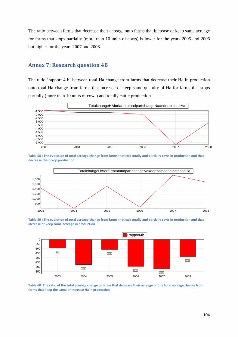
104

The ratio between farms that decrease their acreage onto farms that increase or keep same acreage

for farms that stops partially (more than 10 units of cows) is lower for the years 2005 and 2006

but higher for the years 2007 and 2008.


The ratio ‘rapport 4 b’ between total Ha change from farms that decrease their Ha in production

onto total Ha change from farms that increase or keep same quantity of Ha for farms that stops

partially (more than 10 units of cows) and totally cattle production.

Table 58 : The evolution of total acreage change from farms that exit totally and partially cows in production and that


Table 59 : The evolution of total acreage change from farms that exit totally and partially cows in production and that

increase or keep same acreage in production


farms that keep the same or increase Ha in production

TotalchangeHAforfarmtotandpartchangeNaanddecreaseHa

2003 2004 2005 2006 2007 2008

-1,500-2,000-2,500-3,000-3,500-4,000-4,500-5,000-5,500-6,000

TotalchangeHAforfarmtotandpartchangeNakeepsameandincreaseHa

2003 2004 2005 2006 2007 2008

1,800

1,600

1,400

1,200

1,000

800

Rapport4b

2003 2004 2005 2006 2007 2008

0

-50

-100

-150

-200

-250

-300

-350

2003

2004

2005

2006

2007

2008

105

Annex 8: Research question 5 - Investigation over difference in

percentage change

Farms that decrease cows in production by more than 5 %


acreage by less than -5%






Table 64 : Among farms that decrease the number of cows by more than -10 %, the number of farm per year that

decrease acreage by less than -10%


2003 2004 2005 2006 2007 2008

5,000

4,800

4,600

4,400

4,200

4,000

3,800

3,600

3,400


2003 2004 2005 2006 2007 2008

1,500

1,400

1,300

1,200

1,100

1,000

900

800

700

rationumber_farms5

2003 2004 2005 2006 2007 2008

0.45

0.4

0.35

0.3

0.25

0.2

0.15

0.1

0.05

0

2003 2004

2005

2006

2007

2008


2003 2004 2005 2006 2007 2008

4,200

4,000

3,800

3,600

3,400

3,200

3,000

2,800

2,600

106


decrease acreage by more than -10%









2003 2004 2005 2006 2007 2008

900

850

800

750

700

650

600

550

500

450

400

rationumber_farms10

2003 2004 2005 2006 2007 2008

0.3

0.25

0.2

0.15

0.1

0.05

0

2003

2004

2005

2006

2007

2008


2003 2004 2005 2006 2007 2008

2,5002,4002,3002,2002,1002,0001,9001,8001,7001,6001,5001,400


2003 2004 2005 2006 2007 2008

500

450

400

350

300

250

107






Table 71 : Among farms that decrease the number of cows by more than -30%, the number of farm per year that decrease




rationumber_farms20

2003 2004 2005 2006 2007 2008

0.25

0.2

0.15

0.1

0.05

0

2003

2004

2005

2006

2007

2008


2003 2004 2005 2006 2007 2008

1,600

1,500

1,400

1,300

1,200

1,100

1,000

900


2003 2004 2005 2006 2007 2008

360340320300280260240220200180160140

rationumber_farms30

2003 2004 2005 2006 2007 2008

0.25

0.2

0.15

0.1

0.05

0

2003

2004

2005

2006

2007

2008

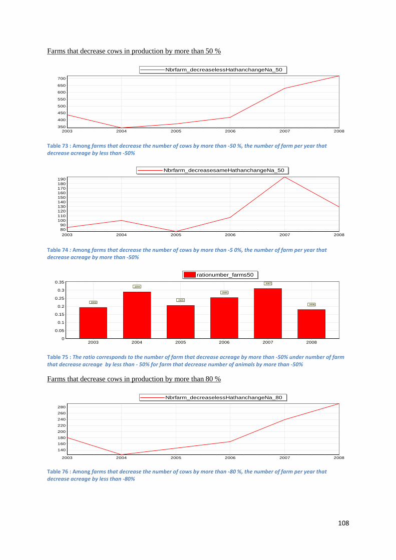
108




Table 74 : Among farms that decrease the number of cows by more than -5 0%, the number of farm per year that








2003 2004 2005 2006 2007 2008

700

650

600

550

500

450

400

350


2003 2004 2005 2006 2007 2008

190180170160150140130120110100

9080

rationumber_farms50

2003 2004 2005 2006 2007 2008

0.35

0.3

0.25

0.2

0.15

0.1

0.05

0

2003

2004

2005

2006

2007

2008


2003 2004 2005 2006 2007 2008

280

260

240

220

200

180

160

140

109






2003 2004 2005 2006 2007 2008

110

100

90

80

70

60

50

rationumber_farms80

2003 2004 2005 2006 2007 2008

0.550.5

0.450.4

0.350.3

0.250.2

0.150.1

0.050

2003

2004

2005

2006

2007

2008

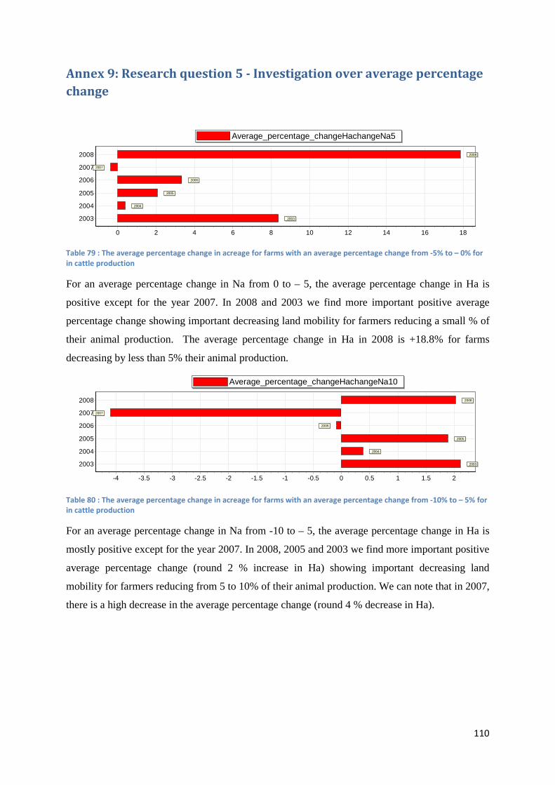
110

Annex 9: Research question 5 - Investigation over average percentage

change

Table 79 : The average percentage change in acreage for farms with an average percentage change from -5% to – 0% for

in cattle production

For an average percentage change in Na from 0 to – 5, the average percentage change in Ha is

positive except for the year 2007. In 2008 and 2003 we find more important positive average

percentage change showing important decreasing land mobility for farmers reducing a small % of

their animal production. The average percentage change in Ha in 2008 is +18.8% for farms

decreasing by less than 5% their animal production.

Table 80 : The average percentage change in acreage for farms with an average percentage change from -10% to – 5% for

in cattle production

For an average percentage change in Na from -10 to – 5, the average percentage change in Ha is

mostly positive except for the year 2007. In 2008, 2005 and 2003 we find more important positive

average percentage change (round 2 % increase in Ha) showing important decreasing land

mobility for farmers reducing from 5 to 10% of their animal production. We can note that in 2007,

there is a high decrease in the average percentage change (round 4 % decrease in Ha).

Average_percentage_changeHachangeNa5

181614121086420

2003

2004

2005

2006

2007

2008

2003

2004

2005

2006

2007

2008


21.510.50-0.5-1-1.5-2-2.5-3-3.5-4

2003

2004

2005

2006

2007

2008

2003

2004

2005

2006

2007

2008

111

Table 81 : The average percentage change in acreage for farms with an average percentage change from -20% to – 10%

for in cattle production


mostly negative except for the year 2006 and 2003. For this category it seems that decreasing land

mobility can be observed more significantly in 2006 and 2005 compare to year 2004.




mostly negative except for the 2003. For this category it seems that decreasing land mobility can

be observed more significantly in 2006 and 2008 compare to year 2004 but not compare to year

2003.



For an average percentage change in Na from -50 to –30, the average percentage change in Ha is

higher in 2005, reflecting decreasing land mobility in 2005. But for this category with high


0.50-0.5-1-1.5-2-2.5-3-3.5-4-4.5-5-5.5

2003

2004

2005

2006

2007

2008

2003

2004

2005

2006

2007

2008


10.50-0.5-1-1.5-2-2.5-3-3.5-4-4.5-5-5.5-6-6.5-7-7.5

2003

2004

2005

2006

2007

2008

2003

2004

2005

2006

2007

2008


0-1-2-3-4-5-6-7-8-9-10-11

2003

2004

2005

2006

2007

2008

2003

2004

2005

2006

2007

2008

112

average percentage change in animal production, average percentage change in Ha is also high in

2008.




higher in 2005, 2007 and 2008, reflecting decreasing land mobility in 2005, 2007 and 2008

compare to the year 2004.




higher in 2006, 2007 and 2008, reflecting decreasing land mobility in 2005, 2007 and 2008

compare to the year 2004.


0-2-4-6-8-10-12-14-16-18-20-22-24

2003

2004

2005

2006

2007

2008

2003

2004

2005

2006

2007

2008


0-2-4-6-8-10-12-14-16-18-20-22-24

2003

2004

2005

2006

2007

2008

2003

2004

2005

2006

2007

2008

assessing the impact of decoupled payments on the mobility...

Documents