Journal of Biomolecular NMR, 19: 305–320, 2001.KLUWER/ESCOM© 2001Kluwer Academic Publishers. Printed in the Netherlands.

305

Assessing the effect of conformational averaging on the measured valuesof observables

Roland Bürgi, Jed Pitera & Wilfred F. van Gunsteren∗Laboratory of Physical Chemistry, Swiss Federal Institute of Technology Zürich, CH-8092 Zürich, Switzerland

Received 1 September 2000; Accepted 22 December 2000

Key words:averaging, molecular dynamics, NOE,3J -coupling constant, saddle-point approximation

Abstract

Experiment and computer simulation are two complementary tools to understand the dynamics and behavior ofbiopolymers in solution. One particular area of interest is the ensemble of conformations populated by a particularmolecule in solution. For example, what fraction of a protein sample exists in its folded conformation? How oftendoes a particular peptide form an alpha helix versus a beta hairpin? To address these questions, it is importantto determine the sensitivity of a particular experiment to changes in the distribution of molecular conformations.Consequently, a general analytic formalism is proposed to determine the sensitivity of a spectroscopic observable tothe underlying distribution of conformations. A particular strength of the approach is that it provides an expressionfor a weighted average across conformational substates that is independent of the averaging function used. Theformalism is described and applied to experimental and simulated nuclear Overhauser enhancement (NOE) and3J -coupling data on peptides in solution.

Introduction

Statistical mechanics shows that any simple observ-able of a macroscopic system (a solution of proteinmolecules) can be described as an ensemble averageover microscopic states (individual protein moleculesin that solution). When considering an observable ata particular time, this ensemble average is carried outlinearly over all of theN molecules in the observedvolume:

〈A〉 = 1

N

N∑i=1

Ai. (1)

Since the value of observableA is usually somefunction of the molecular conformationr, A(r), thesum over molecules above is typically re-cast as anintegral over possible conformationsr weighted by theprobability of each conformationp(r):

〈A〉 =∫A(r)p(r) dr, (2)

∗To whom correspondence should be addressed. E-mail:wfvgn@igc.phys.chem.ethz.ch

where∫p(r) dr = 1. (3)

Equation 2 shows how to calculate the value ofan ensemble average once the distributionp(r) of mi-croscopic states in a sample is known. Unfortunately,it is often straightforward to determine〈A〉 from theexperiment, while the underlying distributionp(r) isexperimentally inaccessible since the experiment isboth a time- and ensemble-average over molecularconformations. In contrast, molecular dynamics andMonte Carlo simulations provide a direct sampling ofmicroscopic statesr with probability p(r) but oftenhave difficulty reaching the time scales necessary toyield converged values of〈A〉.

For bulk materials and macroscopic properties ofcondensed matter systems, we are not particularlyinterested in the distribution of microscopic states.However, this is not the case for proteins and otherbiomolecules. For these systems, conformation is in-timately linked to function – for example, it canmodulate ligand affinity, as in theT andR states ofhemoglobin (Moffat et al., 1979) or affect the access

306

of substrates to an enzyme active site, like the openand closed forms of hexokinase (Bennett and Steitz,1980) or the gated states of acetylcholinesterase (Zhouet al., 1998). To understand the biological function it isessential to understand the populations and dynamicsof these conformational substates.

Towards this end, theoretical and experimentalstudies of biomolecules are rapidly converging. Whilethe first computer simulation of protein dynamicswas 3 picoseconds in simulated duration (McCammonet al., 1977), today routine protein simulations spanseveral nanoseconds (Stocker et al., 2000) and typi-cal peptide simulations reach 50 to 100 nanoseconds(Daura et al., 1999b). In parallel, experimental meth-ods have increased enormously in both time resolutionand molecular resolution. Single molecule fluores-cence spectroscopy is providing information on thebehaviour (and variations) of individual enzymes andproteins (Nie et al., 1994).

Recent long-timescale simulations of proteins andpeptides have underscored the fact that it is possiblefor an ensemble of populations (or a trajectory of asingle molecule) to yield ensemble averages compat-ible with a particular microscopic state even thoughthe simulated ensemble contains only fractional popu-lations of the particular state in question. For example,Daura et al. (1999a) have shown that molecular dy-namics trajectories of aβ-heptapeptide populated aparticular ‘folded’ conformation only 50% of the timeat 340 K, yet yielded no NOE distance bound violationgreater than 0.06 nm.

This problem has actually been well known in thespectroscopic community for some time. While it isextensively discussed in the NMR literature (Jardet-zky and Roberts, 1981), attempts to connect NMRobservables to the underlying conformational ensem-ble have concentrated on simplified models of themolecular geometry. For example, Braun et al. (1981)showed that a uniform distribution of interatomic dis-tances would yield an NOE signal if at least 10% ofthe distribution falls within a threshold distance. Forthe relationship between3J -coupling constants andtorsion angles, Jardetzky considered the influence ofaveraging over several discrete conformations on theapparent value of several NMR observables (Jardet-zky, 1980), and showed that a particular value of anobservable is often compatible with a range of distrib-utions over several different conformations. It is wellknown that certain ranges of3J -coupling constantsprovide limited structural information due to the de-generacy or multiple-valuedness of the Karplus curve

relating3J -coupling constants and the correspondingtorsion angles (Syberts et al., 1987).

However, these analyses have been based on ei-ther uniform distributions or sampling between a smallnumber of discrete model conformations. Consideringmore realistic examples, Bonvin and Brunger (1996)have explored how well a collection of NOEs de-scribes a mix of several realistic conformations of aprotein loop. Similar analyses have been performedusing conformations from a molecular dynamics tra-jectory by Daura et al. (1999a). In both cases it wasshown that the available NOE distance informationwas not able to precisely define the conformationspopulated by the molecule in question. This is asignificant issue given the use of time- and ensemble-averaging schemes in modern NMR refinement pro-tocols (Bonvin et al., 1994). More detailed compar-isons have been performed between experimental andsimulated cross-relaxation rates and order parameters(Bruschweiler et al., 1992; Philippopoulos and Lim,1994; Beutler et al., 1996), but primarily with theintent of reproducing the experimental observations.

If more observations are available than the numberof relevant degrees of freedom, it becomes possibleto use statistical techniques of sensitivity analysis orcomponent analysis to infer the underlying probabil-ity distribution or potential (Ho and Rabitz, 1993;Lazarides et al., 1994; Utz, 1998). In the single ob-servable case we consider, such techniques are notapplicable since they require more data than parame-ters. As a result we make use of a simple parametricsensitivity analysis in this paper.

Although the problem of connecting the value of aspectroscopic observable with its underlying ensemblehas probably been discussed the most in the context ofNMR, it is a general issue for any observation of amolecule that undergoes some sort of averaging (vanGunsteren et al., 1994, 1999). It is particularly cru-cial for thermodynamic interpretations that have beeninferred from spectroscopic data, or for attempts todescribe the structure of highly flexible systems suchas short peptides and protein loops.

The formalism described in this paper permits theanalytic use of realistic probability distributions toestimate the sensitivity of a particular spectroscopicobservable to the composition of the underlying en-semble. We must note, however, that our analysis isrestricted to situations where the kinetics of confor-mational exchange do not themselves influence theobservable measured for each molecule. For NMR,this corresponds to the case where exchange between

307

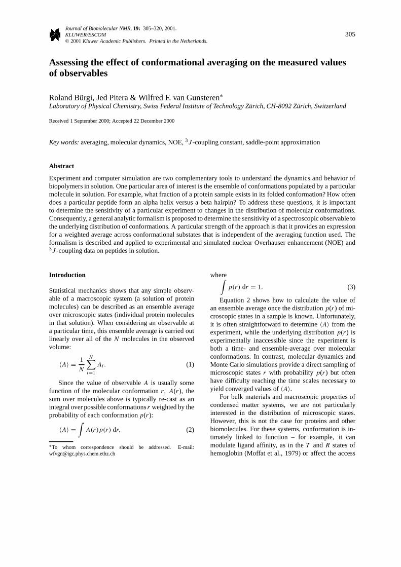
Figure 1. Double-well potentialf (r) (Equation 5) described by the parametersr1,1r, and1f .

conformations is slow with respect to overall rotationbut fast with respect to the macroscopic relaxation rate(T2).

While we describe the averaging problem in termsof single observables, a more complex case often oc-curs where several observables are measured for aparticular sample. For example, cyclic structures arecommonly determined by considering all measured3J -coupling values around the cycle and selecting theconformation that best fits this set of data. Thoughwe do not deal with this case explicitly, it is straight-forward to extend our single-observable formalism tothe realm of two or more observables. If the observ-ables all correspond to the same degree of freedom,r, then when taken as a whole they can significantlyconstrain the underlying probability distributionp(r).Finding the bounds onp(r) becomes a question ofsolving a system ofN equations, one for each observ-able but all with common parameters describing theunderlying distribution. When the observables applyto different degrees of freedom (e.g.,〈A1〉 and 〈A2〉with independent distributionsp(r1) andp(r2)), farless information can be derived. In the case of non-linear averaging, the formalism described herein canbe used to estimate the minimum fractional populationnecessary to generate a particular ensemble average. Ifthe sum of these minimum fractions is greater than 1,

it implies that the underlyingp(r) probability distrib-utions must be somewhat correlated. If the sum is lessthan unity, however, all the individual ensemble aver-ages can be satisfied even if the underlying probabilitydistributions are uncorrelated.

Sensitivity analysis

This section has the purpose of estimating analyti-cally the effect of different distributions and averagingmethods on observables. Using the saddle-point ap-proximation (see Appendix A), we can calculate aweighted average for a distribution together with ageneral averaging function, where the weights do notdepend on the averaging function itself. This providesus with a function that can be readily used in the sen-sitivity analysis of a given observable by analysing thederivatives of the weighted average with respect to theparameters describing the distribution.

In this work, we focus on the analysis of a bimodaldistribution. For many questions asked in a sensitivityanalysis, considering a bimodal distribution is suffi-cient – the sensitivity of an averaging function towardsshifting two maxima of a distribution with respect toeach other can be analysed. If more complex distrib-

308

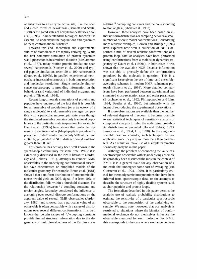
Figure 2. (∂g/∂(1r))/g for the bimodal distribution (Equations 4 and 5) and averaging Equation 13 withβ = 100. (A) shows the derivativeas a function ofr1 and1r at1p = 0; in (B), the value of1p is 1. (C) shows the derivative as a function of1r and1p at r1 = 2, and (D) as afunction ofr1 and1p at1r = 2.

utions have to be considered, the formalism is easilyexpandable to general distributions.

Weighted average in a bimodal distribution

For simplicity, we will denote the degree of freedomover which is averaged byr. The averaging func-tion defining the observable will be calledg(r). It iseasiest to analyse a bimodal distributionp(r) of theconformational degree of freedomr, as the numberof parameters describing such a distribution is suffi-ciently small. The bimodal distributionp(r) can bedescribed by a double-well effective potentialf (r)(see Figure 1) through

f (r) = −1

βlogp(r), (4)

whereβ is one of the parameters describing the dis-tributionp(r). The potentialf (r) is described by thefunction

f (r) = 1

41r3

{(r − r1)2

[1r3(r − r1−1r)2

+41f(31r − 2r + 2r1)]}+ a0, (5)

for 0 ≤ r ≤ ∞. Its functional form (Equation 5) hasbeen chosen such thatf ′(r1) = f ′(r1 + 1r) = 0,f (r1) = a0, andf (r1 + 1r) = a0 + 1f . In order toobtain a proper probability distributionp(r) throughEquation 4, it is required thatp(r) satisfies Equation 3.In other words,a0 has to be chosen such that

∞∫0

e−βf (r) dr = 1. (6)

This condition yields, using the saddle-point approx-imation Equation 17 considering both minima of thepotential,

a0 = 1

βlog

[2√

π

β1r (A+ B)

], (7)

with

A = 1√1r4+ 121f

(8)

B = e−β1f√1r4− 121f

(9)

309

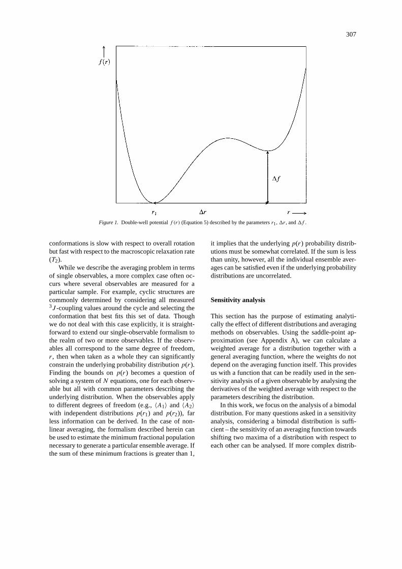
Figure 3. (∂g/∂(1p))/g for the bimodal distribution (Equations 4 and 5) and averaging Equation 13 withβ = 100. (A) shows the derivativeas a function ofr1 and1r at1p = 0; in (B), the value of1p is−0.98. (C) shows the derivative as a function of1r and1p at r1 = 2, and (D)as a function ofr1 and1p at1r = 2.

Note that the condition

|1f | < 1r4

12(10)

must be fulfilled. Thus we have four parameters de-scribing the bimodal distribution:r1, 1r, 1f , andβ.

The average quantityg can then be calculated,using the saddle-point approximation, as

g = Ag(r1)+ Bg(r1 +1r)A+ B . (11)

In the special case of1f = 0, this leads to

g = 12 (g(r1)+ g(r1 +1r)) . (12)

Extension to general distributions

The formalism described above can easily be extendedto general distributions. For each new peak, two addi-tional parameters have to be introduced in a similarway as for the bimodal distribution, describing thevertical and horizontal distances of the maxima withrespect to each other. Due to the saddle point approxi-mation, each peak will contribute as a summand to the

average. Needless to say that the formalism cannot beapplied to a distribution without a single peak.

Application of the formalism to NOE distances

In this section, the derived formulae are used to inves-tigate the effect of ther−6 averaging when obtaining avalue for an observable, i.e., for the case

g(r) = r−6. (13)

Analysis of ther−6 average

To analyse the influence of ther−6 averaging in adouble-well potential, it is of interest to look at thebehaviour of the derivatives∂g/∂(1r) and∂g/∂(1f )for several cases. However, as1f is not very easy tointerpret directly, we will introduce the parameter

1p = p(r1 +1r)− p(r1)p(r1)

= e−β1f − 1, (14)

310

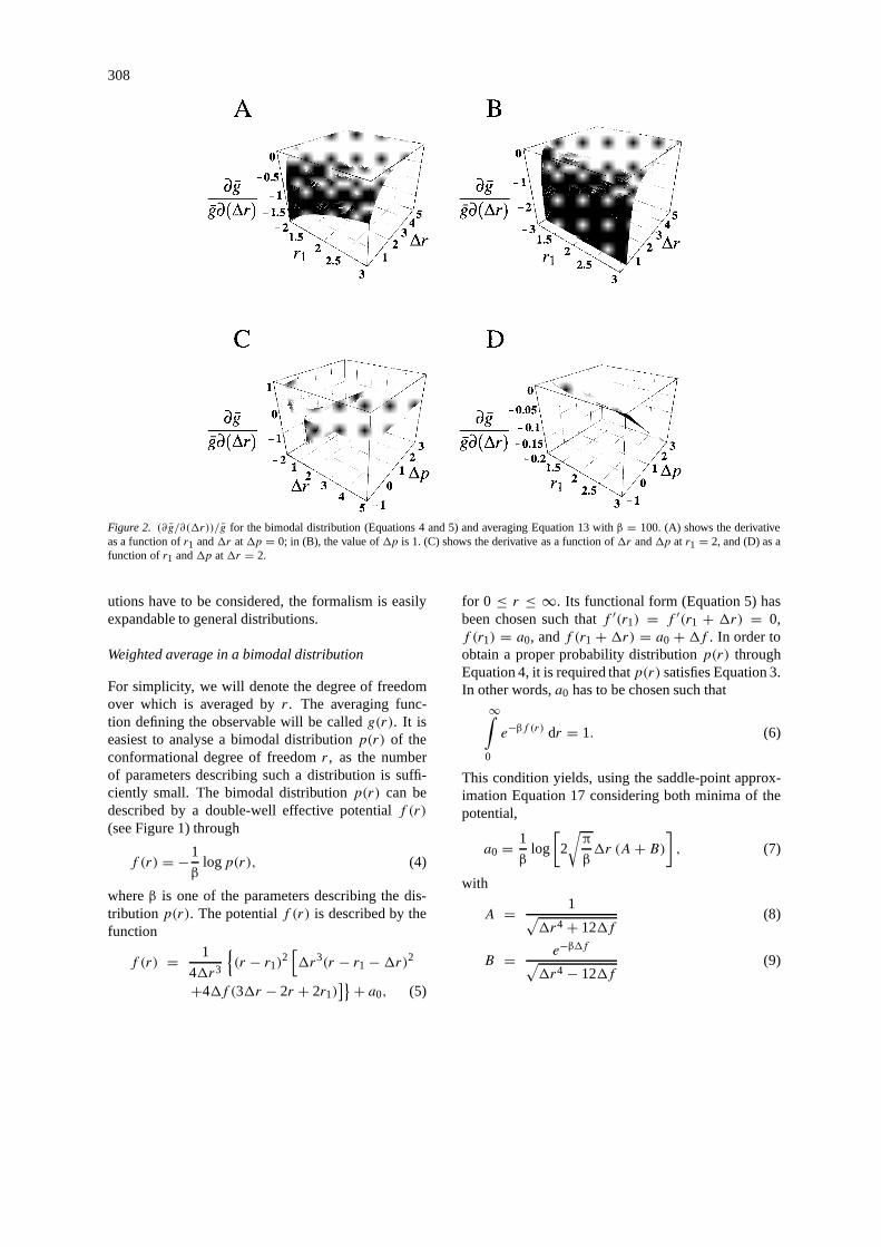
Figure 4. Parameter values defining bimodal distance distributions. All points in the surface(r1,1r,1p) yield the averageg = 2−6 asdetermined by Equations 4–11 and 14.

Table 1. Four example interatomic distance distributions taken from two MD simulations (Bürgi et al.,2001; Daura et al., 1998, 1999b). Indicated are the parametersr1, 1r, 1f , andβ (Equations 4 and5) of a bimodal distribution fitted to the simulated distributions. The last five lines show ther−6

weighted average distancer (MD) calculated over the simulated distribution, the average distancer

(SPA) calculated using the saddle-point approximation (SPA) to the bimodal distribution, the upperbound distancer (exp.) derived from NOE experiments, and the value of the derivative of the average

g =⟨r−6

⟩with respect to1r and1p of the bimodal distribution

Atom pair Octapeptide in DMSO 150 ns Heptapeptide in MeOH 200 ns

1CB1-2HN 2CB2-5HN 2HN-5HCB 3HN-5HCB

r1 (nm) 0.318 0.455 0.314 0.364

1r (nm) 0.117 0.125 0.440 0.405

1f (nm4) −1.12× 10−6 −1.23× 10−6 2.16× 10−4 8.54× 10−5

β (nm−4) 8.72× 105 9.25× 104 3.62× 103 4.50× 103

r (MD) (nm) 0.335 0.487 0.357 0.402

r (SPA) (nm) 0.371 0.495 0.336 0.397

r (exp.) (nm) 0.404 0.471 0.330 0.340∂g

g∂(1r)(nm−1) −4.82 −2.65 0.186 0.091

∂gg∂(1p)

−0.154 −0.132 −0.650 −0.538

311

Figure 5. Distance distributionsp(r) that yield an averageg =⟨r−6

⟩= 2−6. The parameter values areβ = 100 for (A–I),1r = 2 for (A–F),

1p = 5 for (G–I), andr1 = 2.0,1p = −0.99 (A), r1 = 1.87,1p = −0.5 (B), r1 = 1.79,1p = 0 (C), r1 = 1.59,1p = 2 (D), r1 = 1.46,1p = 5 (E), r1 = 1.34,1p = 10 (F),r1 = 1.45,1r = 3 (G),r1 = 1.45,1r = 4 (H), r1 = 1.45,1r = 5 (I).

where p(r) denotes the distribution of the degreeof freedomr, and therefore1p denotes the relativeheight difference of the two peaks of the bimodaldistribution.

The derivative(∂g/∂(1r))/g for β = 100 isshown in Figure 2.

According to Equation 10,|1f | < 1r4/12 mustbe fulfilled. At the border surface1f = − log(1 +1p)/β = 1r4/12, the value of the derivative ofgwith respect to1r goes to infinity for negative1pand to minus infinity for positive1p. Qualitatively, allthe derivatives are negative. That means, when chang-ing to a bigger1r, the average

⟨r−6

⟩gets smaller,

i.e. the average distance⟨r−6

⟩−1/6gets bigger. From

Figure 2A,1p = 0, we can see that changing1rhas hardly any influence on the average unless1r isvery small. The average is not defined at1r = 0,and therefore, the derivative goes to minus infinity. If1p = 1 (Figure 2B), the average is not defined for

1r ≤ 0.537. Otherwise, the surface looks the same asthe one in Figure 2A. The same situation is observed inFigure 2C (r1 = 2): the derivative is nearly zero untilit approaches the disallowed area for1r. Figure 2D(1r = 2) shows clearly what we have seen already inFigure 2A–C, namely that the value of the derivativeonly slightly depends on the choice ofr1 and1p aslong as1r � (12|1f |)1/4.

Furthermore, if we want to extend this analysis to

the observable⟨r−6

⟩−1/6, we must consider the Taylor

expansion(g + ∂g

∂(1r)1(1r)

)−1/6 =g−1/6− g−7/6 1

6∂g

∂(1r)1(1r)+ · · ·

(15)

Therefore, the influence of a slight change in1r onthe average distance is even reduced more.

The dependence of(∂g/∂(1r))/g on r1 and1rfor negative1p is not separately shown because, as

312

Figure 6. Four examples of atom-atom distance distributions taken from two MD simulations. (A) shows the distribution of the distance1CB1-2HN between residues 1 and 2 and (B) the distribution of the distance 2CB2-5HN between residues 2 and 5 of an octapeptide in DMSO(150 ns at 298 K) (Bürgi et al., 2001), (C) the distribution of the distance HN to H-CB between residues 2 and 5 and (D) the distribution of thecorresponding atoms of residues 3 and 5 of aβ-heptapeptide in methanol (200 ns at 340 K) (Daura et al., 1998, 1999b). The solid curves are thedistribution of the distances as taken from the MD simulations, the dashed curves are obtained by fitting a bimodal distribution to the simulateddistributions. The solid line indicates the value of ther−6 average over the simulated distribution, the dashed line the average as calculatedusing the saddle-point approximation, and the dashed-dotted line the upper bound derived from NOE measurements.

can be inferred from Figures 2C and 2D (r1 = 2 and1r = 2 respectively), the influence of changing1r isalways about zero for negative1p.

The derivative(∂g/∂(1p))/g for β = 100 isshown in Figure 3. As in the previous case, the valuesof the derivatives hardly depend onr1 and1r, as longas1r � (12|1f |)1/4. The value of the derivative isaround−1 for 1p = −0.98 (Figure 3B) and around−0.5 for1p = 0 (Figure 3A). It vanishes for larger1p (Figures 3C and 3D), as then the first maximumin the distribution dominates the average completely.

We can conclude that ther−6 average is even moreinsensitive to changes in1p than to changes in1r.

Analysing the space of parameter values that yieldthe same average is even more interesting than inves-tigating the derivatives ofg. The space that yields theaverageg = 2−6 is shown forβ = 100 in Figure 4.For each pair1r and1p, a value forr1 can be foundthat yields the averageg = 2−6, as long as Equation10 is fulfilled. As1p approaches−1, r1 approachesthe value 2. This is clear, as in this case, there wouldbe only one maximum in the distribution. It is also

313

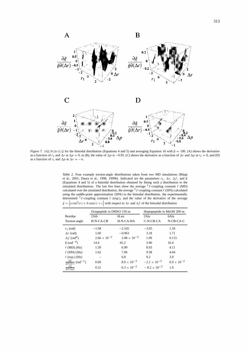
Figure 7. (∂g/∂(1r))/g for the bimodal distribution (Equations 4 and 5) and averaging Equation 16 withβ = 100. (A) shows the derivativeas a function ofr1 and1r at1p = 0, in (B), the value of1p is−0.95. (C) shows the derivative as a function of1r and1p at r1 = 0, and (D)as a function ofr1 and1p at1r = −π.

Table 2. Four example torsion-angle distributions taken from two MD simulations (Bürgiet al., 2001; Daura et al., 1998, 1999b). Indicated are the parametersr1, 1r, 1f , andβ

(Equations 4 and 5) of a bimodal distribution obtained by fitting such a distribution to thesimulated distributions. The last five lines show the average3J -coupling constantr (MD)calculated over the simulated distribution, the average3J -coupling constantr (SPA) calculatedusing the saddle-point approximation (SPA) to the bimodal distribution, the experimentallydetermined3J -coupling constantr (exp.), and the value of the derivative of the average

g =⟨a cos2(r)+ b cos(r)+ c

⟩with respect to1r and1f of the bimodal distribution

Octapeptide in DMSO 150 ns Heptapeptide in MeOH 200 ns

Residue 2Aib 6Leu 2Ala 6Ala

Torsion angle H-N-CA-CB H-N-CA-HA C-N-CB-CA N-CB-CA-C

r1 (rad) −1.94 −2.165 −3.05 1.18

1r (rad) 1.60 −0.963 3.18 1.71

1f (rad4) 2.66× 10−2 2.08× 10−3 1.09 0.115

β (rad−4) 14.4 65.2 3.96 16.4

r (MD) (Hz) 1.59 6.99 8.93 4.11

r (SPA) (Hz) 1.62 7.06 9.58 4.04

r (exp.) (Hz) – 6.8 9.2 3.9∂g

g∂(1r)(rad−1) 0.60 8.0× 10−3 −2.1× 10−3 6.9× 10−2

∂gg∂(1p)

0.31 6.3× 10−2 − 8.2× 10−2 1.9

314

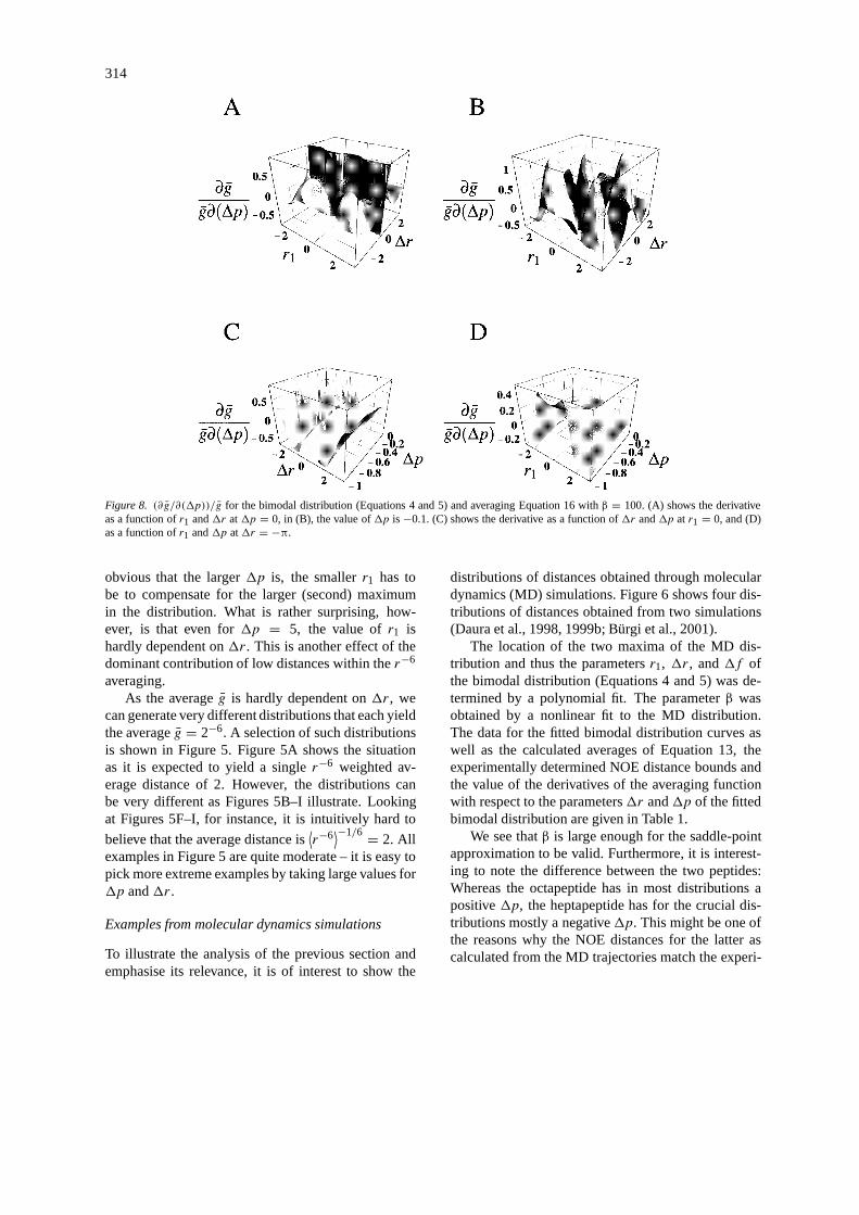
Figure 8. (∂g/∂(1p))/g for the bimodal distribution (Equations 4 and 5) and averaging Equation 16 withβ = 100. (A) shows the derivativeas a function ofr1 and1r at1p = 0, in (B), the value of1p is−0.1. (C) shows the derivative as a function of1r and1p at r1 = 0, and (D)as a function ofr1 and1p at1r = −π.

obvious that the larger1p is, the smallerr1 has tobe to compensate for the larger (second) maximumin the distribution. What is rather surprising, how-ever, is that even for1p = 5, the value ofr1 ishardly dependent on1r. This is another effect of thedominant contribution of low distances within ther−6

averaging.As the averageg is hardly dependent on1r, we

can generate very different distributions that each yieldthe averageg = 2−6. A selection of such distributionsis shown in Figure 5. Figure 5A shows the situationas it is expected to yield a singler−6 weighted av-erage distance of 2. However, the distributions canbe very different as Figures 5B–I illustrate. Lookingat Figures 5F–I, for instance, it is intuitively hard to

believe that the average distance is⟨r−6

⟩−1/6 = 2. Allexamples in Figure 5 are quite moderate – it is easy topick more extreme examples by taking large values for1p and1r.

Examples from molecular dynamics simulations

To illustrate the analysis of the previous section andemphasise its relevance, it is of interest to show the

distributions of distances obtained through moleculardynamics (MD) simulations. Figure 6 shows four dis-tributions of distances obtained from two simulations(Daura et al., 1998, 1999b; Bürgi et al., 2001).

The location of the two maxima of the MD dis-tribution and thus the parametersr1, 1r, and1f ofthe bimodal distribution (Equations 4 and 5) was de-termined by a polynomial fit. The parameterβ wasobtained by a nonlinear fit to the MD distribution.The data for the fitted bimodal distribution curves aswell as the calculated averages of Equation 13, theexperimentally determined NOE distance bounds andthe value of the derivatives of the averaging functionwith respect to the parameters1r and1p of the fittedbimodal distribution are given in Table 1.

We see thatβ is large enough for the saddle-pointapproximation to be valid. Furthermore, it is interest-ing to note the difference between the two peptides:Whereas the octapeptide has in most distributions apositive1p, the heptapeptide has for the crucial dis-tributions mostly a negative1p. This might be one ofthe reasons why the NOE distances for the latter ascalculated from the MD trajectories match the experi-

315

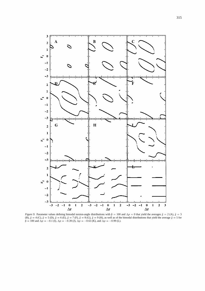
Figure 9. Parameter values defining bimodal torsion-angle distributions withβ = 100 and1p = 0 that yield the averagesg = 2 (A), g = 3(B), g = 4 (C), g = 5 (D), g = 6 (E), g = 7 (F), g = 8 (G), g = 9 (H), as well as of the bimodal distributions that yield the averageg = 5 forβ = 100 and1p = −0.1 (I),1p = −0.39 (J),1p = −0.63 (K), and1p = −0.99 (L).

316

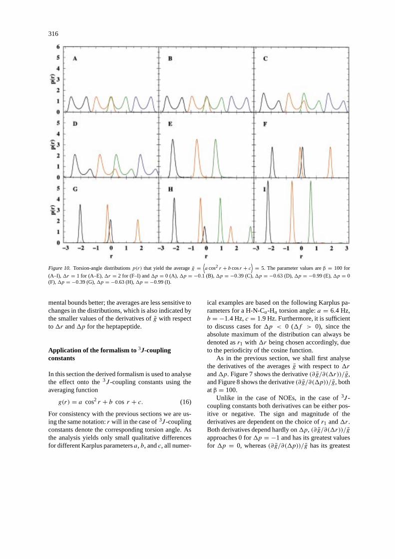
Figure 10. Torsion-angle distributionsp(r) that yield the averageg =⟨a cos2 r + b cosr + c

⟩= 5. The parameter values areβ = 100 for

(A–I), 1r = 1 for (A–E),1r = 2 for (F–I) and1p = 0 (A),1p = −0.1 (B),1p = −0.39 (C),1p = −0.63 (D),1p = −0.99 (E),1p = 0(F),1p = −0.39 (G),1p = −0.63 (H),1p = −0.99 (I).

mental bounds better; the averages are less sensitive tochanges in the distributions, which is also indicated bythe smaller values of the derivatives ofg with respectto1r and1p for the heptapeptide.

Application of the formalism to 3J-couplingconstants

In this section the derived formalism is used to analysethe effect onto the3J -coupling constants using theaveraging function

g(r) = a cos2 r + b cos r + c. (16)

For consistency with the previous sections we are us-ing the same notation:r will in the case of3J -couplingconstants denote the corresponding torsion angle. Asthe analysis yields only small qualitative differencesfor different Karplus parametersa, b, andc, all numer-

ical examples are based on the following Karplus pa-rameters for a H-N-Cα-Hα torsion angle:a = 6.4 Hz,b = −1.4 Hz,c = 1.9 Hz. Furthermore, it is sufficientto discuss cases for1p < 0 (1f > 0), since theabsolute maximum of the distribution can always bedenoted asr1 with 1r being chosen accordingly, dueto the periodicity of the cosine function.

As in the previous section, we shall first analysethe derivatives of the averagesg with respect to1rand1p. Figure 7 shows the derivative(∂g/∂(1r))/g,and Figure 8 shows the derivative(∂g/∂(1p))/g, bothatβ = 100.

Unlike in the case of NOEs, in the case of3J -coupling constants both derivatives can be either pos-itive or negative. The sign and magnitude of thederivatives are dependent on the choice ofr1 and1r.Both derivatives depend hardly on1p, (∂g/∂(1r))/gapproaches 0 for1p = −1 and has its greatest valuesfor 1p = 0, whereas(∂g/∂(1p))/g has its greatest

317

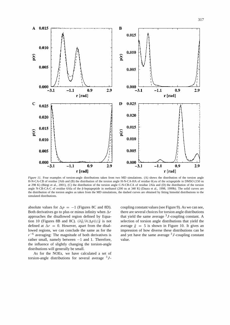
Figure 11. Four examples of torsion-angle distributions taken from two MD simulations. (A) shows the distribution of the torsion angleH-N-CA-CB of residue 2Aib and (B) the distribution of the torsion angle H-N-CA-HA of residue 6Leu of the octapeptide in DMSO (150 nsat 298 K) (Bürgi et al., 2001), (C) the distribution of the torsion angle C-N-CB-CA of residue 2Ala and (D) the distribution of the torsionangle N-CB-CA-C of residue 6Ala of theβ-heptapeptide in methanol (200 ns at 340 K) (Daura et al., 1998, 1999b). The solid curves arethe distribution of the torsion angles as taken from the MD simulations, the dashed curves are obtained by fitting bimodal distributions to thesimulated distributions.

absolute values for1p = −1 (Figures 8C and 8D).Both derivatives go to plus or minus infinity when1rapproaches the disallowed region defined by Equa-tion 10 (Figures 8B and 8C).(∂g/∂(1p))/g is notdefined at1r = 0. However, apart from the disal-lowed regions, we can conclude the same as for ther−6 averaging: The magnitude of both derivatives israther small, namely between−1 and 1. Therefore,the influence of slightly changing the torsion-angledistributions will generally be small.

As for the NOEs, we have calculated a set oftorsion-angle distributions for several average3J -

coupling constant values (see Figure 9). As we can see,there are several choices for torsion angle distributionsthat yield the same average3J -coupling constant. Aselection of torsion angle distributions that yield theaverageg = 5 is shown in Figure 10. It gives animpression of how diverse these distributions can beand yet have the same average3J -coupling constantvalue.

318

Examples from molecular dynamics simulations

As for the r−6 averaging, we illustrate the analysisof the previous section with torsion-angle distributionsobtained from the same two simulations (Bürgi et al.,2001; Daura et al., 1998, 1999b). Figure 11 shows fourexamples of torsion-angle distributions taken fromthese simulations. To obtain the bimodal distributions,the same fitting procedure as for the distance distri-butions was applied. The data for the fitted bimodaldistribution curves as well as the calculated averagesof Equation 16, the experimentally determined3J -coupling constants and the value of the derivatives ofthe averaging function with respect to the parameters1r and1p of the bimodal distribution are shown inTable 2.

Even thoughβ is much smaller for all exampletorsion-angle distributions than it was for the NOEdistances, the saddle-point approximation still seemsto be quite accurate. All four averages are very insen-sitive to changes of the distributions. All derivativesof the average with respect to the distribution para-meters are of the order of 10−3 to 101. For smallchanges in the distribution, the average will not changesignificantly.

Conclusions

We have presented a formalism to analyse a generalaveraging functiong(r), which represents an observ-able, in terms of sensitivity of the average of theobservable to small changes in the distribution of thedegree of freedomr. The formalism is based on thesaddle-point approximation, which yields as the aver-age over a bimodal distribution a weighted average,where the weights do not depend on the averagingfunction. Therefore, it is straightforward to calculatederivatives of the weighted average with respect to theparameters of the bimodal distribution.

For the two examples of averaging functions givenhere,g(r) = r−6 (NOEs) andg(r) = a cos2(r) +b cos(r) + c (3J -coupling constants), it was shownthat the averages are not very sensitive to a variety ofchanges in the distribution ofr. Furthermore, we havecalculated the range of parameters that yield the sameaverage value and shown the diversity of distributionsthat yield the same average value. For the cases wehave studied, this implies that an experimentally aver-aged value does not contain much information on theunderlying distribution of molecular conformations.

It is our expectation that the approach outlined inthis paper will be generally useful as a quantitativeway both to assess experimental data or simulationresults and as a way to deepen and make more pre-cise the connection between computer simulations andexperimental data.

Acknowledgements

Financial support was obtained from the Schweiz-erischer Nationalfonds, project number 21-57069.99,which is gratefully acknowledged. R.B. thanks DrXavier Daura for providing his data on the heptapep-tide and Prof. Herman Berendsen for useful discus-sions on the subject.

Appendix A: Saddle-point approximation

The formulation of the theorem as well as the prooffollow the ideas given in (Jänich, 1983).Theorem.Let g(r) and f (r) be functions that aresufficiently many times differentiable on an interval(a, b). The casesa = −∞, b = +∞ are also al-lowed. The functionf (r) should be real and havea non-degenerate absolute minimum atr0 ∈ (a, b).Furthermore, there should existδ > 0 and ε > 0 sothat f (r) is decreasing monotonically on the interval(r0 − ε, r0) and increasing monotonically on the in-terval (r0, r0 + ε) and thatf (r) ≥ f (r0)+ δ for all routside the interval(r0−ε, r0+ε). g(r) should be cho-sen such thatg(r0) 6= 0 and that

∫ ba |g(r)|e−βf (r) dr

exists for aβ = β0 (and therefore for allβ ≥ β0). Thefollowing expression is then valid:

b∫a

g(r)e−βf (r) dr =

g(r0)e−βf (r0)

[√2π

f ′′(r0) · β + O

(1

β3/2

)](17)

Proof. All contributions of the integral outside theinterval (r0 − ε, r0 + ε) can be neglected, as theirabsolute value is≤ e−δβeδβ0 · ∫ ba |g(r)|e−β0f (r)dr.These contributions are therefore absorbed in the er-ror termO(β−3/2). f (r) can be expanded aroundr0:f (r) = f (r0) + 1

2f′′(r0)(r − r0)2 + higher-order

terms. Let us callf ′′(r0) = c2, sincef (r0) is anon-degenerate minimum. If we also expandg(r) =

319

Figure 12. Conditions forf (r) are thatf (r) ≥ f (r0)+ δ for all r outside the interval(r0 − ε, r0 + ε).

g(r0)+ c1(r − r0)+ (r − r0)2ψ(r) aroundr0, all thatremains to be solved is the integralr0+ε∫r0−ε

g(r)e−βf (r0)− 12βc2(r−r0)2 dr =

g(r0)r0+ε∫r0−ε

e−βf (r0)− 12βc2(r−r0)2 dr

+c1

r0+ε∫r0−ε

(r − r0)e−βf (r0)− 12βc2(r−r0)2 dr

+r0+ε∫r0−ε

(r − r0)2ψ(r)e−βf (r0)− 12βc2(r−r0)2 dr.

(18)

The first term is approximated by

g(r0)e−βf (r0)

r0+ε∫r0−ε

e− 12βc2(r−r0)2 dr ' g(r0)e−βf (r0)

∞∫−∞

e− 12βc2r2

dr = g(r0)e−βf (r0)√

2π

βc2 .

(19)

The second term vanishes, as the integrand is anti-symmetric aroundr0. Sinceψ(r) is bounded in theinterval(r0 − ε, r0 + ε), i.e. ψ(r) ≤ c2 with c2 > 0,the third term is approximated by

e−βf (r0)r0+ε∫r0−ε

(r − r0)2ψ(r)e− 12βc2(r−r0)2 dr

' c2e−βf (r0)

∞∫−∞

r2e− 12βc2r2

dr = c2βc2

√2πβc2 .

(20)

Therefore, the third term is also included in the errortermO(β−3/2).

References

Bennett, W.S. and Steitz, T.A. (1980)J. Mol. Biol., 140, 183–230.Beutler, T.C., Bremi, T., Ernst, R.R. and van Gunsteren, W.F. (1996)

J. Phys. Chem., 100, 2637–2645.Bonvin, A.M.J.J. and Brunger, A.T. (1996)J. Biomol. NMR, 7, 72–

76.Bonvin, A.M.J.J., Boelens, R. and Kaptein, R. (1994)J. Biomol.

NMR, 4, 143–149.Braun, W., Boesch, C., Brown, L.R., Go, N. and Wüthrich, K.

(1981)Biochim. Biophys. Acta, 667, 377–396.Bruschweiler, R., Roux, B., Blackledge, M., Griesinger, C.,

Karplus, M. and Ernst, R.R. (1992)J. Am. Chem. Soc., 114,2289–2302.

Bürgi, R., Daura, X., Mark, A., Bellanda, M., Mammi, S., Peggion,E. and van Gunsteren, W.F. (2001)J. Pept. Res., 57, 107.

Daura, X., Antes, I., van Gunsteren, W.F., Thiel, W. and Mark, A.(1999a)Proteins, 36, 542–555.

Daura, X., Jaun, B., Seebach, D., van Gunsteren, W.F. and Mark,A.E. (1998)J. Mol. Biol., 280, 925–932.

Daura, X., van Gunsteren, W.F. and Mark, A.E. (1999b)Proteins,34, 269–280.

Ho, T.S. and Rabitz, H. (1993)J. Phys. Chem., 97, 13447–13456.Jänich, K. (1983)Analysis für Physiker und Ingenieure: Funk-

tionentheorie, Differentialgleichungen, spezielle Funktionen.Springer-Verlag, Berlin.

Jardetzky, O. (1980)Biochim. Biophys. Acta, 621, 227–232.Jardetzky, O. and Roberts, G.C.K. (1981)NMR in Molecular

Biology, Academic Press, New York, NY, Chapter 4.Lazarides, A.A., Rabitz, H. and McCourt, F.R.W. (1994)J. Chem.

Phys., 101, 4735–4749.McCammon, J.A., Gelin, B.R. and Karplus, M. (1977)Nature, 267,

585–590.Moffat, K., Deatherage, J.F. and Seybert, D.W. (1979)Science, 206,

1035–1042.Nie, S.M., Chiu, D.T. and Zare, R.N. (1994)Science, 266, 1018–

1021.Philippopoulos, M. and Lim, C. (1994)J. Phys. Chem., 98, 8264–

8273.Stocker, U., Spiegel, K. and van Gunsteren, W.F. (2000)J. Biomol.

NMR, 18, 1–12.

320

Syberts, S.G., Maerki, W. and Wagner, G. (1987)Eur. J. Biochem.,164, 625–635.

Utz, M. (1998)J. Chem. Phys., 109, 6110–6124.van Gunsteren, W.F., Bonvin, A.M.J.J., Daura, X. and Smith, L.J.

(1999) InStructure Computation and Dynamics in Protein NMR(Eds, Krishna, N.R. and Berliner, L.J.), Vol. 17 ofBiol. MagneticResonance, Plenum Publishers, New York, NY, pp. 3–35.

van Gunsteren, W.F., Brunne, R.M., Gros, P., van Schaik, R.C.,Schiffer, C.A. and Torda, A.E. (1994)Methods Enzymol., 239,619–654.

Zhou, H.X., Wlodek, S.T. and McCammon, J.A. (1998)Proc. Natl.Acad. Sci. USA, 95, 9280–9283.