assessing the damage potential in pretensioned freight
TRANSCRIPT

®
The contents of this report reflect the views of the authors, who are responsible for the facts and the accuracy of the information presented herein. This document is disseminated under the sponsorship of the Department of Transportation
University Transportation Centers Program, in the interest of information exchange. The U.S. Government assumes no liability for the contents or use thereof.
Assessing the Damage Potential in Pretensioned Bridges Caused by Increased Truck Loads Due to Freight Moments (Phase II)
Report # MATC-KSU: 252 Final Report
Robert J. Peterman, Ph.D., P.E.Martin K. Eby Distinguished Professor in EngineeringDepartment of Civil EngineeringKansas State University
Steven F. Hammerschmidt, M.S.C.E Graduate Research Assistant
2011
A Cooperative Research Project sponsored by the U.S. Department of Transportation Research and Innovative Technology Administration
MATC
The contents of this report reflect the views of the authors, who are responsible for the facts and the accuracy of the information presented herein. This document is disseminated under the sponsorship of the U.S. Department of Transportation’s University
Transportation Centers Program, in the interest of information exchange. The U.S. Government assumes no liability for the contents or use thereof.
25-1121-0001-252

Assessing the Damage Potential in Pretensioned Bridges Caused by Increased Truck Loads
Due to Freight Moments (PHASE II)
Robert J. Peterman, Ph.D., P.E.
Martin K. Eby Distinguished Professor in
Engineering
Department of Civil Engineering
Kansas State University
Steven F. Hammerschmidt, M.S.C.E.
Graduate Research Assistant
Department of Civil Engineering
Kansas State University
A Report on Research Sponsored by
Mid-America Transportation Center
University of Nebraska-Lincoln
August 2011

Technical Report Documentation Page
1. Report No. 25-1121-0001-252
2. Government Accession No.
3. Recipient's Catalog No.
4. Title and Subtitle
Assessing the Damage Potential in Pretensioned Bridges Caused
by Increased Truck Loads Due to Freight Movements (Phase II)
5. Report Date August, 2011
6. Performing Organization Code
7. Author(s) Robert J. Peterman, Ph.D., P.E. and Steven F. Hammerschmidt
8. Performing Organization Report
No.
25-1121-0001-252
9. Performing Organization Name and Address Mid-America Transportation Center
2200 Vine St.
PO Box 830851
Lincoln, NE 68583-0851
10. Work Unit No. (TRAIS)
11. Contract or Grant No.
12. Sponsoring Agency Name and Address Research and Innovative Technology Administration 1200 New Jersey Ave., SE Washington, D.C. 20590
13. Type of Report and Period
Covered Draft Report,
14. Sponsoring Agency Code MATC TRB RiP No. 18460
15. Supplementary Notes
16. Abstract With aging and deterioration of bridges, evaluation of existing conditions of their structural elements becomes vital to
engineers and public officials when deciding how to repair or replace the structures. The ability to obtain necessary
information on these conditions is often expensive and time consuming, especially for concrete bridges where the
reinforcement is not available for inspection. Employing the surface-strain relief method could allow for accurate
evaluation of aged or damaged prestressed members.
The surface-strain relief method was developed to measure initial or pre-existing strains in a concrete member. It involves
relieving the strain in the member and measuring the change in strain. Two methods were tested in this study—one used a
linear electrical-resistance strain gage and a three-inch-diameter diamond concrete core bit to cut around the gage, and the
second method used a laser-speckle imaging device and a diamond cutting wheel to create notches perpendicular to the axis
of maximum strain. Both methods measured the change in strain and related it to within 10% of the actual fse. The
method of cutting notches and the laser-speckle imaging device provided a simpler method to be implemented in the field,
while the coring method achieved a higher level of accuracy and precision.
17. Key Words
18. Distribution Statement
19. Security Classif. (of this
report) Unclassified
20. Security Classif. (of this page) Unclassified
21. No. of
Pages 95
22. Price

iii
Table of Contents
Chapter 1 Introduction .................................................................................................................... 1
Chapter 2 Literature Review ........................................................................................................... 4
2.1 Similar Methods to the Surface-Strain Relief Method ......................................................... 4
2.1.1 ASTM E837 Standard Test Method for Determining Residual Stresses by the Hole-
Drilling Method ...................................................................................................................... 4
2.1.2 National Airport Pavement Test Facility Core-Ring Strain Gage Test Procedure ........ 5
2.1.3 Factors Affecting the Hole-Drilling Method ................................................................. 9
2.1.4 Core Trepanning Method ............................................................................................. 10
2.1.5 Summary of Similar Residual Stress Measurement Procedures .................................. 12
2.2 Destructive and Semi-Destructive Methods to Determine Average Prestress Force ......... 12
Chapter 3 Test Specimens ............................................................................................................. 16
3.1 Design and Casting of Rectangle Beams ............................................................................ 16
3.2 Rectangle Specimen Material Properties ............................................................................ 27
3.3 T-Beam Specimen Geometries Properties .......................................................................... 28
3.4 T-Beam Specimen Material Properties ............................................................................... 29
Chapter 4 Surface-Strain Relief Method ....................................................................................... 30
4.1 Measurement of Strain ........................................................................................................ 30
4.1.1 Strain Measurements with Strain Gages ...................................................................... 31
4.1.2 Laser-Speckle Imaging (LSI) Device .......................................................................... 33
4.2 Coring Process .................................................................................................................... 41
4.3 Notching Process ................................................................................................................ 44
4.4 Calculation of the Average Prestress Force ........................................................................ 46
4.5 Determining the Modulus of Elasticity of the Concrete ..................................................... 47
Chapter 5 Finite Element Models ................................................................................................. 49

iv
5.1 Rectangle Beam Models ..................................................................................................... 49
5.1.1 Model Parameters ........................................................................................................ 49
5.1.2 Results .......................................................................................................................... 51
5.2 T-beam Models ................................................................................................................... 58
5.2.1 Model Parameters ........................................................................................................ 58
5.2.2 Results .......................................................................................................................... 59
Chapter 6 Determining the Average Prestress Force .................................................................... 62
6.1 ACI Loss Calculations ........................................................................................................ 62
6.2 Use of Whittemore Gage to Determine Losses .................................................................. 63
6.3 Crack-Opening Method to Determine the Average Prestress Force ................................... 64
6.3.1 Crack-Opening Method Setup ..................................................................................... 64
6.3.2 Analysis of Crack-Opening Data ................................................................................. 66
6.4 Results ................................................................................................................................. 73
Chapter 7 Surface-Strain Relief Method Results .......................................................................... 77
7.1 Modulus of Elasticity of the Concrete Beams .................................................................... 77
7.2 Rectangle Beam Results ..................................................................................................... 78
7.2.1 Core Results ................................................................................................................. 79
7.2.2 Notch Results ............................................................................................................... 82
7.3 T-Beam Results ................................................................................................................... 84
7.3.1 Core Results ................................................................................................................. 84
7.3.2 Notch Results ............................................................................................................... 86
7.4 Summary of Results ............................................................................................................ 87
7.5 Temperature Effects ............................................................................................................ 88
Chapter 8 Conclusions and Further Recommendations ................................................................ 91

v
8.1 Conclusions ......................................................................................................................... 91
8.2 Recommendations ............................................................................................................... 92
References ..................................................................................................................................... 93

vi
List of Figures
Figure 2.1 NAPTF Method ............................................................................................................. 6
Figure 2.2 Notches Cut Next to Strain Gage .................................................................................. 8
Figure 3.1 Cross Section of Rectangle Beam ............................................................................... 17
Figure 3.2 Longitudinal Section of Rectangle Beam .................................................................... 18
Figure 3.3 a) Crack Former, b) Location of Crack Former .......................................................... 20
Figure 3.4 a) Inserts Cast into Beam, b) Inserts on Gage Bar ...................................................... 21
Figure 3.5 Completed Forms with Strand Tensioned ................................................................... 23
Figure 3.6 Load-Cell Bracket ....................................................................................................... 24
Figure 3.7 Adding Aggregates to Mixer ....................................................................................... 25
Figure 3.8 Adding Water to Mixer ............................................................................................... 25
Figure 3.9 Cross Section of T-Beam............................................................................................. 29
Figure 3.10 Locations of Crack Formers ...................................................................................... 29
Figure 4.1 a) AE-10 Applied to Surface with Alignment Marks, b) Gage Applied and Clamped in
Place, c) Completed Gage with Connection ......................................................................... 32
Figure 4.2 Laser-Speckle Imaging Device .................................................................................... 33
Figure 4.3 a) Laser-Speckle Imaging From the Concrete Surface, b) Schematic of Laser Speckle
Strain Measurement System.................................................................................................. 34
Figure 4.4 Laser-Speckle Imaging Device with Two-inch Gage Length ..................................... 35
Figure 4.5 Strain Gages Mounted on Channel .............................................................................. 36
Figure 4.6 Channel Loaded ........................................................................................................... 37
Figure 4.7 Laser Speckle Compared to Strain Gage ..................................................................... 38
Figure 4.8 Concrete Specimen in Load Frame ............................................................................. 39
Figure 4.9 (a) Laser-Speckle Imaging Device Mounting Brackets, (b) Laser-Speckle Imaging
Device Mounted to Beam ..................................................................................................... 40
Figure 4.10 a) After the Core Has Been Removed, b) Core Intact ............................................... 44
vii
Figure 5.1 Finite Element Model Restraint................................................................................... 50
Figure 5.2 (a) Stress Distribution across Core, (b) Stress Distribution across Notch ................... 52
Figure 5.3 Plot of Stress along Length of Strain Gage ................................................................. 53
Figure 5.4 Plot of Stress on Surface of Cores ............................................................................... 54
Figure 5.5 Plot of Stress between Notches ................................................................................... 55
Figure 5.6 Plot of Varying Length of Notches ............................................................................. 56
Figure 5.7 Plot of Varying the Spacing of Notches ...................................................................... 57
Figure 5.8 a) Core Parallel to Bottom of Beam, b) Core Perpendicular to Web, c) Notch .......... 59
Figure 5.9 Surface Stress Comparing Direction of Core .............................................................. 61
Figure 6.1 Beam Setup .................................................................................................................. 65
Figure 6.2 Deflection Measurement Setup ................................................................................... 66
Figure 6.3 LVDT Mounted to Measure Crack Width ................................................................... 66
Figure 6.4 Graph of Bilinear Response ......................................................................................... 69
Figure 6.5 Linear Regression Lines Plotted on Graph .................................................................. 70
Figure 7.1 Reinforcement Affecting Strain Relief on the Surface of the Core ............................. 85

viii
List of Tables
Table 3.1 Mix Proportions ............................................................................................................ 19
Table 3.2 Stress in Each Strand .................................................................................................... 27
Table 3.3 Compressive Strengths of the Concrete Mixes ............................................................. 28
Table 5.1 Calculated Stresses and Percent Relieved across Cores ............................................... 54
Table 5.2 Calculated Stresses at a Spacing of 3.5", Length of 3", and Varying Depth ................ 55
Table 5.3 Calculated Stresses at a Notch Depth 1”, Spacing of 3.5”, and Varying Length ......... 57
Table 5.4 Calculated Stresses at a Depth of 1", Length of 3", and Various Spaces ..................... 57
Table 5.5 T-Beam Calculated Stresses ......................................................................................... 60
Table 6.1 Applied Loads to Open Crack ...................................................................................... 72
Table 6.2 fse Based on Losses ........................................................................................................ 74
Table 6.3 Results of Crack-Opening Procedure for Beam 2 ........................................................ 74
Table 6.4 Summary of Crack-Opening Procedure ........................................................................ 75
Table 6.5 Summary of All Stress Determination Methods ........................................................... 76
Table 6.6 T-Beam Calculated fse ................................................................................................... 76
Table 7.1 Modulus of Elasticity .................................................................................................... 78
Table 7.2 Measured Strains on Beam 1a Using the Coring Procedure ......................................... 79
Table 7.3 Measured Strains on Beam 1b Using the Coring Procedure ........................................ 80
Table 7.4 Measured Strains on Beam 2a Using the Core Procedure ............................................ 80
Table 7.5 Measured Strains on Beam 2b Using the Core Procedure ............................................ 80
Table 7.6 Calculated fse and Percent Error for the Core Method .................................................. 81
Table 7.7 Measured Strains on Beam 1b Using the Notch Procedure .......................................... 82
Table 7.8 Measured Strains on Beam 2b Using the Notch Procedure .......................................... 83
Table 7.9 Measured Strains on Beam 2a Using the Notch Procedure .......................................... 83

ix
Table 7.10 Calculated fse and Percent Error for the Notching Method ......................................... 83
Table 7.11 Measured Strains on T-Beam 1 Using the Coring Procedure ..................................... 85
Table 7.12 Measured Strains on T-Beam 2 Using the Coring Procedure ..................................... 85
Table 7.13 Calculated fse and Percent Error for the Coring Method ............................................. 86
Table 7.14 Measured Strains on T-Beam 2 Using the Notching Procedure ................................. 86
Table 7.15 Calculated fse and Percent Error for the Coring Method ............................................. 87
Table 7.16 Core Temperatures ...................................................................................................... 89
Table 7.17 Increase in Strain Due to Temperature Fluctuations .................................................. 89

x
Acknowledgements
The authors would like to thank the Mid-America Transportation Center (MATC) for
funding this project, and Dr. Mustaque Hossain, MATC Associate Director at Kansas State
University, for his encouragement and guidance throughout this project.

xi
Abstract
With aging and deterioration of bridges, evaluation of existing conditions of their
structural elements becomes vital to engineers and public officials when deciding how to repair
or replace the structures. The ability to obtain necessary information on these conditions is often
expensive and time consuming, especially for concrete bridges where the reinforcement is not
available for inspection. Employing the surface-strain relief method could allow for accurate
evaluation of aged or damaged prestressed members.
The surface-strain relief method was developed to measure initial or pre-existing strains
in a concrete member. It involves relieving the strain in the member and measuring the change
in strain. Two methods were tested in this study—one used a linear electrical-resistance strain
gage and a three-inch-diameter diamond concrete core bit to cut around the gage, and the second
method used a laser-speckle imaging device and a diamond cutting wheel to create notches
perpendicular to the axis of maximum strain. Both methods measured the change in strain and
related it to within 10% of the actual fse. The method of cutting notches and the laser-speckle
imaging device provided a simpler method to be implemented in the field, while the coring
method achieved a higher level of accuracy and precision.

1
Chapter 1 Introduction
In North America, many prestressed concrete bridges were built over the past five
decades. Many of these bridges, including rural bridges on county roads, are approaching the
end of their design life, or have been subjected to larger loads and heavier traffic demands,
making them deficient and in need of repair. To preserve the structural integrity of the bridges
and safety of the public, inspections need to be conducted. With prestressed members, visible
inspections may not be sufficient in determining the condition of the structure due to
environmental and time-dependent losses of the prestressing force. Therefore, engineers need a
reliable method to determine the remaining prestress force in a member during routine
inspections and rehabilitation, or when retrofitting the structure.
Current evaluation methods involve visual inspections and/or instrumenting the structure
with strain gages, then applying a known load to the structure, and measuring the change in
strain due to the applied load. The load is then varied and models are created from the gathered
data, and finally strains in members can be extrapolated from the models. While these methods
are accurate, they only capture strains induced by an applied load and not initial or residual
stresses in the members. Two methods exist to determine the remaining prestress force in a
member, but both are semi-destructive and difficult to conduct in an existing structure. The first
method involves applying a load to generate flexural cracks; instrumenting the cracks with
displacement transducers, strain gages, or similar devices; loading the structure once more; and
determining the moment needed to open the crack to produce zero concrete tension at the
instrumented crack. The second method involves removing concrete from around the tendon,
and then cutting a wire to measure the deflection of the wire. This deflection can be related to
the stress in the wire and assumes that all wires have similar stress. Again, these methods are

2
semi-destructive, and they are designed for laboratory settings, which would make them difficult
to employ in an existing structure.
As the concern is aging infrastructure, it becomes more important to calculate or measure
the remaining prestress force in existing structures in the field. If the average prestress force in a
member was known, then an accurate analysis could be conducted to determine the existing
stresses in the member as well as the remaining strength of the member. Even more importantly,
it would be possible to calculate the stress range of the member due to fatigue. The average
prestress force provides valuable information when monitoring strength and durability of older or
damaged structures. This would allow bridge owners to make informed decisions about how to
allocate maintenance funds and reduce the inherent risk associated with deteriorating
infrastructure.
When trying to calculate the remaining prestress force for older structures, there is often
limited information that exists on actual design and/or construction and environmental
conditions. Thus assumptions, such as the initial jacking force, have to be made affecting the
accuracy of the analysis. Initially, there may be flaws that are considered insignificant, and
therefore go unnoticed. However, due to time-dependent losses, these flaws may eventually
become critical to the strength of the member. Prestress force is a time-dependent phenomena
influenced by factors such as elastic shortening due to transfer, shrinkage, creep, and relaxation
that occurs after transfer. These losses are calculated based on geometric and mix properties of
the member, along with environmental conditions. Based on research, equations have been
developed to enable the calculation of losses over time. Importantly, these equations are not
exact and are only estimates. They have been developed to provide estimates for many types of
prestressed members.

3
Considering all of the factors mentioned above, a method of surface-strain relief was
developed to accurately measure the remaining prestress force through relief of residual stresses,
while being mostly non-destructive. The method allows bridge members to be monitored over
time to ensure that they are still meeting the design assumptions. As the calculation of the losses
is only an estimate, the surface-strain relief method could lengthen the life of a structure by
providing a level of confidence that the structure can still perform as designed. The surface-
strain relief method provides a cost-effective means to evaluate the condition of the structure,
and places a higher level of certainty on decisions by owners and engineers in regard to the
condition of the structure.
With the success of Phase I, “Development of a Procedure to Determine the Internal
Stresses in Concrete Bridge Members,” Phase II was completed to accurately determine the
existing stresses in concrete prestressed members through a rational and cost-effective means.
Phase I focused on determination of a method of surface-strain relief by dry-coring (Peterman
and Hammerschmidt 2010). This method was developed and tested on post-tensioned concrete
members and compared to theoretical calculations and finite element models. Phase II focused
on the implementation of the method of surface strain relief by dry coring on prestressed
concrete members in a laboratory setting, and determining the accuracy of the method. The
prestress members had multiple strands with varying force, geometry, and production dates.
Results of the surface-strain relief method were compared to the prestress force in the member,
which had been found through the crack-opening procedure. Effectiveness of the method was
evaluated using prestress members with multiple-bonded strands.

4
Chapter 2 Literature Review
Multiple methods similar to surface-strain relief, as proposed for this project, were
researched to find limitations and difficulties encountered with each. Destructive and semi-
destructive methods were researched to use as a basis of comparison, and to accurately determine
the average prestress force in each member.
2.1 Similar Methods to the Surface-Strain Relief Method
Many methods have been proposed to measure residual stresses on the surface of steel
and concrete specimens. The standard to measure residual stresses in steel is found in ASTM
E837. Measurement of residual stresses in concrete members have been researched by the
Federal Aviation Administration’s National Airport Pavement Test Facility (NAPTF) (Guo et al.
2008) and by David G. Marks at the University of Illinois at Urbana-Champaign by modifying
the ASTM E837 hole-drilling method so that it is applicable for concrete members (2009).
Others, like Kesavan, Ravisankar, Parivallal, and Sreeshylam, have created a method to measure
the relaxation around a core or to core around the gage, theoretically relieving all the stress in the
concrete (2005).
2.1.1 ASTM E837 Standard Test Method for Determining Residual Stresses by the Hole-Drilling
Method
According to Vishay Micro-Measurements, residual stresses are developed from virtually
all manufacturing processes, repairs, or modifications (2007). To quantify these residual
stresses, ASTM E837 “Standard Test Method for Determining Residual Stresses by the Hole-
Drilling Method” was developed to measure residual stresses in the critical residual stress
region. The material must be isotropic linear-elastic with residual stresses not exceeding 60% of
the material yield stress, can vary in thickness, and can have non-uniform stress (ASTM E837

5
2009). The stresses are measured near the surface of the material by mounting a rosette strain
gage and drilling a small hole (2 mm in diameter) at the center of it. Residual stresses in the
material surrounding the hole are partially relieved, and the associated relieved strains are
measured at varying depths while drilling and recording the changes using a suitable strain-
recording instrument (ASTM E837 2009). Based on the linear elasticity theory and finite
element models, the residual stresses can be calculated from the difference in strain
measurements and calibration constants found through finite element models. Accuracy of the
method depends on the operator skill and expertise with a precision of ±10%, providing the
stresses are uniform throughout the depth of the hole. When non-uniform stresses are present,
much larger errors result.
2.1.2 National Airport Pavement Test Facility Core-Ring Strain Gage Test Procedure
NAPTF developed a procedure called the core-ring strain gage test, using ASTM E837 as
a basis. The initial objectives were to directly measure residual stresses in concrete beams, and
then to develop a procedure to measure residual stresses in concrete airport pavements. To
complete these objectives, tests were conducted to determine the optimum core-ring size and
depth, and the spacing between the strain gage center and the core-ring edge. The core-ring
strain gage procedure used a single linear-resistance strain gage aligned along the axis of
maximum strain. A core was then drilled at the end of the gage and the relaxation in strain was
measured between the initial strain and the strain measurement after the coring was complete.
Multiple tests were conducted to determine the optimal size of strain gage, core-ring size, and
depth of the core.
NAPTF used both finite element analysis and experimental testing to develop the core-
ring strain gage procedure. Experimental tests were conducted using six-by-six-inch beams, four

6
ft long. By loading the specimens and monitoring the strain, it was found that if each beam was
rotated 90 degrees then the modulus of elasticity was uniform throughout the depth of the
specimen when positioned in this direction. One end of the beam was fixed, and the other end
was loaded 3 inches from the end of the beam using a jack to the specified load of 400 lbs. Then
the beam was cored adjacent to the strain gage (see figure 2.1), varying the depth and recording
the change in strain at each depth. NAPTF concluded that strain gages with a gage length of 1.2
or 0.8 inches worked with a maximum aggregate size of one inch. Three or four inch core rings
provided acceptable results with a one inch core depth. Spacing between the strain gage and the
core-ring edge should be 1 to 2.75 inches (Guo et al. 2008). Finite- element models were created
and compared closely to the experimental results. The finite element models showed larger
strain changes when the core was on the fixed end rather than the end where load was applied.
Therefore, the core ring should be drilled between the gage and the fixed end.
Figure 2.1 NAPTF Method
David G. Marks, from the University of Illinois at Urbana-Champaign, measured residual
stresses in concrete pavements by either coring adjacent to a strain gage or sawing notches at
each end of the strain gage. The project branched from the strain-relaxation technique developed

7
by NAPTF. Both experimental tests and finite element models were conducted to compare the
results of core rings and saw notches.
Beams 6x6 inches and 40 inches long were cast, using a mix design from the Illinois
Department of Transportation. Based on the findings of NAPTF, the beams were rotated 90
degrees for testing, making the side from casting the top side of the beam for testing. This was
done to have a smooth surface for mounting strain gages and a more uniform stiffness in the
beam, according to NAPTF. Both 20 and 30 mm strain gages were used, as suggested by the
NAPTF results, and these were positioned 13 inches from the fixed support. The procedure used
a three-inch-diameter core with water to cool the core bit and reduce the effects of temperature
on the strain readings. Using an NDT James Instruments, Inc. Kwikcore, the core bit was
advanced in 0.25 inch increments to a total depth of 1.25 inches. During the coring process, the
research team recorded strain measurements continuously, and noticed a large change in strain
appeared initially, which generally stabilized after approximately 10 min. The increase in the
strain measurements was due to a temperature increase caused by the difference in the
temperatures of the water and environment. To correct this error, water at the same temperature
of the beam was used and this produced the least amount of strain drift.
A second method was developed which implemented a diamond saw blade, and cut a
notch adjacent to the strain gage (see figure 2.2). A single notch adjacent to the strain gage on
the fixed end of the test specimen, and two notches, one on each side of the strain gage, were
tested. Notching provided a quicker method and eliminated issues with the cooling water affects.
The testing procedure was the same, but instead of the core rings, a circular saw fitted with a
seven-inch masonry saw blade was used. Notches were cut in three passes, moving from a depth
of 0.5 inches, then to 1 inch, and to a final depth of 1.5 inches at a distance of 1.63 inches from

8
the center of the gage. It was found that when sawing notches on each side of the strain gage, all
the stresses were relieved. With both notches cut to a depth of one inch, the strain gage did not
respond noticeably to the applied load, and the gage corresponded to the initial residual stresses
in the beam (Marks 2009).
Figure 2.2 Notches Cut Next to Strain Gage
Marks used finite element models to compare core-ring configurations and single- and
double-notch configurations to the experimental results. Each model created a similar six-by-six
inch beam, cantilevered to induce stresses in it. Linear-strain triangle and quadrilateral elements
were used on the models, with a finer mesh around the notches and a less-fine mesh elsewhere to
reduce the computationally run time. Use of core rings to a depth of one inch provided the same
stress relief as a circular hole, similar to the ASTM E837 procedure. From the finite element
models, a coring ring of three inches at a depth of one inch was sufficient to relieve the stresses.
Full strain relief could be achieved with two notches, and a near-zero surface stress was found
when the notches were at a depth of one inch (Marks 2009). From the experimental and finite
element results, the saw notches provided a full strain relief and did not need additional
calibration constants. Therefore, the residual stresses could be calculated using basic equations.

9
Through finite element modeling, full relaxation occurs when notch depths are 40% of the
distance between the notches (Marks 2009).
2.1.3 Factors Affecting the Hole-Drilling Method
McGinnis (2006) researched three factors that affect the core-drilling method: water-
induced swelling, proximity of steel reinforcement, and differential shrinkage. The core-drilling
method is similar to the ASTM E837 procedure, but instead of measuring strains, this method
measures displacement around the core hole caused by relaxation of the core and relates them to
the residual stresses in the structure.
The core-drilling process uses three points of known location outside of the core to
measure the relieved displacements around the core hole. The relieved displacements are
measured using the digital-image correlation system and calculate radial- and tangential-relieved
displacements of the overall displacement with respect to the center of the core hole. Through a
series of calculations, these displacements are related to in-situ stresses. The digital-image
correlation system images an applied patterned surface to the concrete and then photographs the
object with a pair of digital cameras before and after loading. Using photogrammetric
triangulation principles, the sets of photos are compared and the displacements are calculated.
The field of view is approximately 250 mm wide, and has a displacement resolution of 8 microns
for out-of-plane displacements and better for in-plane displacements (McGinnis 2006).
McGinnis recorded an average error of 28.4% when effects of water-induced swelling,
proximity of steel reinforcement, and differential shrinkage effects were neglected. When
considered and accounted for, an average error in the experiments was 9.5%. It was found that
the presence of reinforcement nearer than 35 mm to the core hole and with a concrete cover of
less than 75 mm causes significant under-prediction in the calculated in-situ stress using the

10
core-drilling method (2006). Water-induced swelling and differential shrinkage created
additional tensile stresses and were added to the actual stresses measured. Using Abaqus
software, models with similar geometry and material properties were created with and without
reinforcement and the results were compared. An error of approximately 20% was found and the
in-situ stress values were adjusted to account for this. Corrections of the water effects are much
more complex and depend on absorption, time of water exposure, porosity, and swelling strain.
These are discussed thoroughly in McGinnis’ dissertation (2006). Differential shrinkage errors
were determined through use of finite element models and data from environmental curing
conditions. From this differential shrinkage, stress profiles were created, and an estimated stress
of 2.55 MPa was found due to differential shrinkage (McGinnis 2006). Correction factors must
be developed from finite element models to account for the additional displacements caused by
reinforcement, water-induced swelling, and differential shrinkage, which makes this procedure
dependent on geometric and material properties of the member.
2.1.4 Core Trepanning Method
Kesavan, Ravisankar, Parivallal, and Sreeshylam developed a procedure, the core
trepanning method, to simplify calculations of residual stress, and made it applicable to
prestressed concrete members currently in service (2005). They accomplished this by coring
around a strain gage positioned along the axis of maximum stress providing a full strain relief.
Their method is unlike other methods where strain gages are positioned around the outer core
hole and the relief around the hole is measured. The core trepanning method places the strain
gage in the middle of the core and measures the relief of the core, which results in a larger
change in strain. With this method, special procedures were developed to waterproof the gage
and create connections to disconnect the lead wires to the strain gages. Through experimental

11
testing a 50-mm-diameter core hole, in combination with a 30 mm electrical resistance strain
gage at a depth of 20 to 30 mm, allowed maximum strain release to occur.
Kesavan, et al. conducted multiple experiments using both pre-tensioned and axially
loaded members to determine the size of strain gage and also the depth of the core. Electrical-
resistance strain gages of 10, 20, and, 30 mm lengths were tested on concrete cubes with no
applied load. Each gage was cored to a total depth of 50 mm (diameter of the core) in 10 mm
increments, recording strain measurements at each increment. The 30 mm gage provided
consistent readings in comparison to the other gages and was found to be within ± 10
microstrain. A second set of tests on axially loaded specimens was run to determine the actual
depth needed to fully release the residual stresses. From coring in 10 mm increments, it was
concluded that maximum released strains occurred between 20 and 30 mm, and that cutting any
deeper was not required (2005).
To further test the method and repeatability on prestress concrete members, the core
trepanning method was used on prestress members by coring around gage positions along the top
and bottom sides of a beam. The measured strains were compared to the recorded strain during
prestressing and revealed that 92% of the applied strain was released through the core trepanning
method (Kesavan et al. 2005). The method was also conducted on a seven-year-old prestressed
T-section that had an initial prestressing force of 360 kN. On the surface of the T-beam, three
cores were taken—one on the top flange and two below the neural axis. With these three cores,
residual stresses were calculated and the residual stress at the neutral axis was interpolated.
Stress at the neutral axis was used to calculate the prestress force in the member, because at the
neutral axis, all bending stresses due to prestress force and gravity load disappear, leaving only

12
the axial compression prestress force. An average prestress force of 285.3 kN was calculated
and found to be in good agreement when taking losses into consideration (Kesavan et al. 2005).
2.1.5 Summary of Similar Residual Stress Measurement Procedures
Looking at the previous research conducted, many methods have been tested and have
shown feasibility in creating a method to measure residual stresses in a prestressed member.
Measuring strain relief around the outside of a hole in steel has provided accurate and repeatable
results. For concrete, this method has also shown that it can be effective, but due to the many
steps involved, complex calculations, and the small strains that are measured, larger error results
make it difficult for implementation outside a laboratory setting. Marks, Kesavan, Ravisankar,
Parivallal, and Sreeshylam have developed two acceptable methods by coring or cutting notches
around a strain gage, which increases the level of strain relief and greatly simplifies the analysis
procedure. Each method uses water to cool the diamond coring bit, which can possibility
damage the strain gage, and introduce swelling in the concrete as McGinnis has found. These
strains due to swelling can be significant, affecting overall accuracy of the method (2005).
2.2 Destructive and Semi-Destructive Methods to Determine Average Prestress Force
Experimental procedures have been developed to accurately determine average prestress
force in a prestress member. One method applies a load and measures the crack width to
determine the load required to first open the crack. This method has proved to be accurate in
determining the average prestress force (fse). Many researchers have used these methods with
variations to determine fse in members of different geometries and ages. Larson, Peterman, and
Rasheed used the procedure to determine fse in T-beams only a few months old (2005); while
Pessiki, Kaczinski, and Wescott tested prestressed I-beams that were removed from an obsolete
bridge (1996). Another method used by Czaderski and Motavalli (2006) removed the concrete

13
surrounding the prestress tendons and measured displacement of the wire as the wires were cut,
and the deformation was related to the stress in the wire.
Larson, Peterman, and Rasheed determined fse in T-beams before strengthening with
carbon fiber reinforcement attached to the bottom of the beams. The researchers pre-cracked
each section with four-point bending, applying an initial load greater than the calculated cracking
moment so a visible crack could be seen, and location of the crack was marked before unloading
the beam. Linear variable differential transducers (LVDTs) were then mounted spanning the
base of the crack. The load was reapplied at the same load rate for an additional 25 cycles to
determine an average cracking moment for the beam. When the crack was just opened, zero
concrete tension resulted at the base of the beam, so the modulus of rupture was assumed to be
zero for calculations of the prestress force. To determine the experimental load needed to just
keep the crack closed and the concrete at zero tension, graphs of load versus deflection were
created. Subsequently, the load was found at the point of end of linearity for cycles two through
ten (2005). Assuming tensile strength of the concrete as zero due to the pre-cracking, linear
elastic analysis of the gross transformed section was used to calculate the average prestressing
stress in the prestressing strands. Larson, Peterman and Rasheed found the experimental fse in
agreement with the calculated PCI losses (2005).
A similar method was conducted on two prestress I-beams taken out of the Shenango
River Bridge on Interstate 80 in Mercer County, Pennsylvania. Pessiki, Kaczinski, and Wescott
(1996) conducted experimental tests on two beams at Lehigh University with each beam loaded
in three separate phases. The purpose of the initial phase was to crack the beam, document the
location of flexural cracks, and instrument the cracks with displacement transducers and strain
gages. Next, the beams were loaded to determine the decompression load, or cracking moment,

14
based on displacement transducers and strain gage measurements. The intention of the final
phase was to load the beam to failure.
During the second phase, the beam was repeatedly loaded and unloaded in a quasistatic
manner in order to determine the decompression load in the bottom of each beam. The
decompression load was determined by three methods—visible observation of the crack opening,
measurement of the crack using LVDTs, and use of surface-mounted strain gages. Examining
the load versus strain curves and the load versus crack width from the LVDTs and strain gages, a
bilinear response was seen. The load versus strain curves showed a proportional increase in load
compared to the strain in the first linear section of the bilinear curve. In the second linear
portion, an increase in load was accompanied by no increase in strain. Once the crack was open,
the strain was no longer transferred across the crack, therefore, no increase in strain.
Linear lines were fitted to each linear segment and the point of intersection was
determined to be the decompression load. The strain gage measurements were found to be
repeatable and varied by no more than three to five percent (1996). The load versus crack width
was analyzed in a similar manner, where the load versus crack width was plotted and typically
showed an increased crack opening with an increasing load. The point when the rate of
increasing load to crack opening changed was taken as the end of linearity; therefore, the
decompression load. The decompression load found using the crack-width data was generally
higher than the decompression load from the strain gages, and visual inspection resulted in the
highest decompression load out of the three values. Pessiki, Kaczinski, and Wescott used the
decompression load determined from the strain gages in the rest of its calculations due to their
consistent and repeatable values (1996).

15
Czaderski and Motavalli (2006) investigated losses of a 38-year-old bridge being
dismantled in southern Switzerland. Five I-beams were removed from the existing bridge, and
each beam consisted of two prefabricated concrete I-beams connected using two post-tensioning
tendons with a parallel wire bundle of 26 or 27 wires. The concrete was removed, exposing the
tendons at five locations along the length of the beam. Once the tendon was visible, the duct and
grouting material was removed, exposing the individual prestressing wires. Aluminum
measurement points were glued on the wires with a spacing of eight inches. Several wires were
instrumented, including interior wires that were accessed by removing some of the exterior
wires. Using a deformeter, a mechanical strain gage, the initial strain measurement was
recorded. The wires were cut, releasing the force in the wires, and the deformeter measured the
change in displacement. Results from the 26 wires showed small deviations in the measured
strains; in addition, when one wire was cut, strain increase in the other wires was minimal
(Czaderski and Motavalli 2006). Calculated and measured tendon force was in good agreement,
and showed cutting a few wires out of each tendon would be sufficient to determine the
remaining post-tensioning force in the member.

16
Chapter 3 Test Specimens
Prestressed beams of varying dimensions are used in bridges and structures, ideally the
surface-strain relief method should be applicable to these various geometries. Steel
reinforcement and the concrete mix designs will vary around the country due to state and local
standards and availability of materials. To test the accuracy of the surface-strain relief method,
cross sections of two types of beams were used—a set of nine-year-old T-beams cast at a
prestressed concrete plant and rectangle beams designed and cast at Kansas State University
(KSU). The beams were initially tested with the crack-opening procedure to determine fse in
each member, and then the surface-strain relief method was used to calculate fse and compare it
to the experimental determination of fse. The beams were designed according to American
Concrete Institute (ACI) and Precast Prestressed Concrete Institute (PCI) codes and standards.
Four beams were cast at KSU with varying stress levels, but with similar concrete properties and
dimensions. The KSU beams were cast in the laboratory where many variables, including
concrete mix, prestress force, and geometry of the member, could be controlled. Whereas the
nine-year-old T-beams represented a member cast by a prestress plant, providing a member that
had incurred losses over time due to environmental conditions.
3.1 Design and Casting of Rectangle Beams
Two sets of beams with rectangle cross sections were designed at KSU to simulate a
beam meeting ACI and PCI code and standards. Each set was designed to contain two beams
cast in series, ensuring that each beam had identical prestress force. These beams used a Kansas
Department of Transportation (KDOT)-approved mix design. The purpose of these beams was
to represent a control beam, limiting the amount of added reinforcement, but still representing a

17
beam with similar stress as one found in a structure. Multiple methods would be used to
determine the prestress force in each beam and verify results of the surface-strain relief method.
Each beam had a cross section 6 inches wide by 12 inches tall and 120 inches long.
Reinforcement in each beam consisted of two ½-inch 270 kips per square inch (ksi) low-
relaxation strand; and two, ½-inch 50 ksi steel reinforcing bars. These were placed with two
inches of concrete cover surrounding the bar in accordance with ACI (ACI 318-08 2008) (see
figure 3.1). To achieve strand stress that represented long-term losses in a member, each strand
was initially stressed to approximately 160 ksi. No shear reinforcement was needed in the beam,
and added stiffness was introduced affecting the surface-strain relief method. Four 3/8-inch steel
stirrups were positioned throughout the beam, one at each end and at the third points to hold the
top bars in place (see figure 3.2). The concrete mix design was a normal-weight mix designed
for KDOT bridge girders. The mix used type III cement with 50% coarse aggregate and 50%
fine aggregate by weight (see table 3.1 for mix proportions). The mix had a design of 28 day
strength of 6000 psi, a 3 inch slump, and 5% air entrainment to meet KDOT specifications. A
release strength of 4200 psi was needed before the beam could be de-tensioned.
Figure 3.1 Cross Section of Rectangle Beam

18
Figure 3.2 Longitudinal Section of Rectangle Beam

19
Table 3.1 Mix Proportions
At the midpoint of the beam, a crack former was embedded as shown in figure 3.3. The
crack former was a 16-gauge stainless steel plate, 5 inches tall and 6 inches wide, with a ½ inch
bend on each side to temporally attach it to the form. One side was covered with duct tape to
prevent the concrete from bonding to the steel. The crack former initiated and controlled the
location of the crack for use with the crack-opening procedure to determine the prestress force in
the beam. The crack former also allowed for the assumption that no concrete tensile stress could
be transferred across the crack. Therefore, the modulus of rupture of the concrete could be
assumed as zero at the midpoint. This greatly simplifies the calculation of the prestress force and
reduces the amount of error and uncertainty in determining the prestress force.
Material Design Quantity
Water 252 lb/yd3
Cement 721 lb/yd3
Large Aggregate 1442 lb/yd3
Small Aggregate 1442 lb/yd3
Daravair 21 mL/yd3
AdvaFlow 450 mL/yd3

20
(a)
(b)
Figure 3.3 a) Crack Former, b) Location of Crack Former
Two 3/8-inch bolts were positioned 2 inches up from the bottom of the beam, and 2
inches from center, to aid in mounting LVDTs for measuring the crack opening at the strand
height. In addition to the bolts at the height of the strand, two threaded brass inserts were
embedded eight inches part, as shown in figure 3.4. Threaded brass inserts, 1/4 x 3/8 inch, were
attached to a gage bar which was then inserted into the forms to be cast into the beam. The bar
was covered with duct tape to prevent it from adhering to the concrete. Using a Whittemore
gage, initial distance between the points was measured and later related to the losses of the
prestress force in the beam.

21
(a)
(b)
Figure 3.4 a) Inserts Cast into Beam, b) Inserts on Gage Bar
The two sets of beams were cast in series, so theoretically there would be the same
prestress force in each beam. This allowed the testing of one beam initially, and the testing of
the second beam after a majority of the creep and shrinkage losses had occurred. According to
Dr. B.C. Punmia, Ashok K. Jain, and Arun K. Jain, 50% of shrinkage occurs within the first
month of curing and 75% takes place in the first 6 months. Similarly, 50% of creep occurs one
month after loading and 75% occurs after 6 months from the initial loading (2003). A minimum
of six months elapsed before testing the second beam from each series to ensure that a majority
of the losses due to creep and shrinkage had occurred. A comparison between the two beams
showed whether any residual stresses were not fully relieved on the core from creep or shrinkage
Threaded Brass Inserts
3/8 inch Bolts
Threaded Brass Inserts
Gage Bar

22
of the concrete due to the prestress force. The beams were design for a maximum compression
stress at the bottom of the beam, while staying within the maximum allowed stress ranges. This
allowed for the assumption that the beams would behave elastically.
Wooden forms were built with inside dimensions of 6 inches by 12 inches. The forms
were continuous with a total length of 21 ft. Two beams were cast end to end in the forms,
leaving a six inch space between the beams to allow for de-tensioning. Each strand was initially
jacked to one kip to align the forms to the center of the strand, and place the stirrups and top bars
in place. Once all the forms and steel were in place, each strand was jacked to 75% of the tensile
strength of the strand, or 31 kips. Figure 3.5 shows the overall setup of the forms with all the
steel placed in the forms and the strands tensioned to 31 kips. Each strand had a load cell on one
end to verify the load in the strand. A bracket was designed to allow a load cell to be positioned
on each end and not interfere with the other strand position two inches away (see figure 3.6).
Using a post-tensioning jack with an electric hydraulic pump, each strand was stressed
individually and then a chuck was seated to hold the force in the strand. The final stress in each
strand was approximately 160 ksi after the seating losses of 15%.

23
Figure 3.5 Completed Forms with Strand Tensioned
Beam 2
Beam 1
(2) ½” 270 ksi
Strands
Strand 1

24
Figure 3.6 Load-Cell Bracket
The beams were cast using a trailer-mounted portable drum mix with a capacity of one
cubic yard. Fifteen cubic ft of concrete was batched for each set of beams, which included
taking a slump and air test, and making four 6 x 12-inch cylinders and nine 4 x 8-inch cylinders.
All materials were weighed out into barrels using a 2,000 pound capacity crane scale.
Aggregates were weighed out the night before casting and sealed in 55 gallon barrels to prevent
loss of moisture. Three samples were taken from the aggregate piles to calculate moisture
content in the aggregates. Once the moisture content was known, corrections were made to the
mass of the aggregates and to the amount of water needed for the mix. Aggregates were added
to the mixer by first dumping them into a hopper that then guided the materials into the mixer
(see figure 3.7). Next, cementitious materials were added, while the water and admixtures were
added last (see figure 3.8). The water was added using a pressurized water tank where the mass
of the water could be measured.
Load Cell
Chuck
Bracket
Strand 2
Chuck
Plate to Center
Strand in Load Cell

25
Figure 3.7 Adding Aggregates to Mixer
Figure 3.8 Adding Water to Mixer
Once the concrete had been thoroughly mixed, it was dumped into wheelbarrows and
samples were taken to determine slump and air entrainment. Following ASTM C143 (2000) and
C138 (2001) a slump of three inches was found for each mix and an air entrainment of five
Drum Mixer
Hopper
Drum Mixer
Pressured
Water Tank

26
percent was determined. Concrete cylinders were made for determining average compressive
strength and modulus of elasticity of the mix, and these cylinders were created following ASTM
C31 (2003). The cylinders were cured next to the beam to represent the beam properties and not
the ultimate strength potential of the mix. When placing concrete in the beam, a concrete
vibrator was used to consolidate the concrete around the reinforcement and to create a smooth
surface for mounting gages on the sides of the beams. A wooden hand trowel was used to finish
the top surface of each beam, and then the beams were covered with wet burlap followed by
plastic until the next day when the beams were de-tensioned.
The forms were removed the next morning, and three concrete cylinders were broken to
determine an average strength of the concrete. For the first set of beams, the strength was 6350
psi and for the second set it was 5970 psi, well above the required 4200 psi. Before de-
tensioning, the load at each load cell was recorded and represented the force in each strand. The
Whittemore gage was used to measure the initial distance between the brass inserts. De-
tensioning was done using an oxy-acetylene torch, cutting one wire in the first strand followed
by a wire in the second strand and continuing this process until all wires were cut. This
prevented a sudden release which could cause spalling or other damage to the beam. Next, the
beams were picked up and placed on blocks at each end. Using the Whittemore gage, readings
were taken on the brass inserts to record initial losses in each beam and to find the average
prestress stress in each strand. Stresses in each strand during casting and after de-tensioning are
shown in table 3.2. Initial stress values are given for each strand from the load cell positioned on
each strand. The post de-tensioning values are from the Whittemore measurements and represent
the average prestressing force in each strand. The beams were then transported to a storage area
where they were allowed to cure and be prepared for testing.

27
Table 3.2 Stress in Each Strand
3.2 Rectangle Specimen Material Properties
The four rectangle beams were cast in two separate pours using the same materials and
design mix. Each mix had a 28 day design strength of 6000 psi and a release strength of 4200
psi. Table 3.3 shows the average compressive strength at release and 28 days. Each mix had
very similar average compressive strengths as shown in the table. The average modulus of
elasticity was determined at the time of the surface-strain relief method and was found to be
3,528 ksi for the first pour and 3,750 ksi for the second pour. The prestressing steel had a tensile
strength of 270 ksi and a modulus of elasticity of 28,500 ksi. Other steel, such as the top bars
and stirrups, had a tensile strength of 50 ksi with a modulus of elasticity of 29,000 ksi.
Beams 1a and 1b Initial Pull Before CastingAfter
De-tensioning
Strand 1 208.6 176 163.9
Strand 2 205.7 172.5 163.9
Beams 2a and 2b
Strand 1 205.3 161.8 143.1
Strand 2 185.0 164.7 143.1
Average Stress (ksi)

28
Table 3.3 Compressive Strengths of the Concrete Mixes
3.3 T-Beam Specimen Geometries Properties
The prestressed concrete T-beams were cast at Prestressed Concrete, Inc. (PCI) in
Newton, Kansas, in March of 2002. The T-beams had a top flange 18 inches wide and 4 inches
deep, with a tapered web 4 inches wide at the bottom and a total depth of 14 inches (see figure
3.9). The T-beam had two straight 3/8-inch 270 ksi low-relaxation strands, one 2-inches up and
another 4-inches up from the bottom and jacked to a stress of 202.5 ksi. Additional mild
reinforcement of D4-welded-wire reinforcement was placed in the beam at 1.25, 3, 4, and 7
inches from the top. Shear reinforcement was provided in the form of D4-welded-wire
reinforcement placed four inches on center in the flange and D6-welded-wire reinforcement
placed four inches on center in the web. Crack formers were embedded in the bottom of the
beam to initiate a crack in the web of the beam at three locations—mid-span and 3.5 ft from each
side of mid-span (see figure 3.10).
Pour At Release 28 Day
1 6350 7490
2 5970 7390
Design 4200 6000
Average Compressive Strength

29
Figure 3.9 Cross Section of T-Beam
Figure 3.10 Locations of Crack Formers
3.4 T-Beam Specimen Material Properties
The T-beams were produced in 2002 at a prestressed plant in Kansas. The plant provided
concrete strength measurements through standard cylinder testing. The average 28-day strength
was measured at 7,040 psi. Average modulus of elasticity was obtained from the crack-opening
procedure and found to be 3,285 ksi. The 3/8-inch strand used in the beams had a tensile
strength of 270 ksi and an elastic modulus of 28,300 ksi. The additional mild steel reinforcement
had a tensile strength of 80 ksi and an elastic modulus of 29,000 ksi (Larson 2002).

30
Chapter 4 Surface-Strain Relief Method
The surface-strain relief method determines residual strain on the surface of a member
and relates it to residual stresses in the member. For prestressed members, residual stress can be
considered primarily due to prestressing force applied to the beam. The surface-strain relief
method has four main steps:
1) Measuring initial strain,
2) Coring or cutting notches,
3) Measuring relaxation of the concrete, and
4) Relating relaxation of the concrete to the average prestress force.
Two methods were explored to measure surface strain—traditional linear electrical-
resistance strain gages (ERSG) and a laser-speckle imaging (LSI) device. Initially, residual
stresses on the surface were relieved by coring around the strain gage, but upon further research,
a method of notching was used and showed promising results. The core and notches were cut to
varying depths to determine optimal depth and were compared with finite element models. The
strain was measured after each incremental core or notch depth. Change in strain was assumed
to be the relief of the residual stress and was used to calculate average prestress force in the
member.
4.1 Measurement of Strain
Two methods were used to measure surface strain: the traditional linear electrical-
resistance strain gage and the LSI device. The linear-resistance strain gages were used with a
concrete diamond coring bit and the notches technique. Phase I showed minimal error with a
strain gage and core, so the effectiveness of the notch procedure was compared to the coring
process. The LSI device was not used with the core because it measures the strain over a larger

31
area, requiring a larger core bit. A larger core would provide many disadvantages to the method,
and limit possibilities and applications. With a larger core, location of the core would be
affected. With a three-inch core, the center of the core must be approximately two inches up
from the bottom. This ensures that there is enough space to prevent the core bit from breaking
out the concrete at the bottom of the beam, as well as provide the necessary space to mount the
guide. With the larger gage length and development of the notches, the LSI device provided an
opportunity to simplify the method.
With either method, the linear-resistance strain gage or the LSI device, the strain is only
measured in one direction. In order to get the least error and the largest change in strain, the
strain gage or the optical device must be positioned parallel to the axis of maximum strain. For
the purposes of this project, the remaining prestress force was being investigated, so the gages
were positioned along the centroid of the prestress strand.
4.1.1 Strain Measurements with Strain Gages
Linear-resistance strain gages from Vishay Micro-Measurements were used for the
majority of the testing due to the reliability and known accuracy of the strain gages. Vishay EA-
06-20CBW-120 strain gages were used with a gage length of 2 inches and a resistance of 120
ohms. Following Vishay Micro-Measurements Tech Note 505-4, two inch strain gages were
used due to the size of the aggregates in the concrete mix design (Vishay Micro-Measurements
2007).
To mount the strain gages, locations of the gages were marked on the surface of the
beam, and this area was lightly ground down to remove any laitance from the surface. Following
Vishay Micro-Measurements Tech Note 611 (2010) for mounting strain gages on concrete
surfaces, AE-10 epoxy was used to fill in any voids in the surface of the concrete and provide a

32
smooth surface to mount the gages. Vishay Micro-Measurements Bulletin B-137 (2010) was
followed to prepare the surface and to mount the gage to the AE-10. Once the gages were
installed, short lead wires, approximately two inches in length, were soldered to the gage. A
four-pin terminal block connector was soldered on the other end to allow the gage to be quickly
connected and disconnected during the coring process. M-coat polyurethane coating was applied
over the gages to prevent damage to the gage, and for further protection, microcrystalline wax
was applied over the M-coat. Type I/II silicone was used to hold the terminal block in place and
prevent movement during coring (see figure 4.1).
(a) (b)
(c)
Figure 4.1 a) AE-10 Applied to Surface with Alignment Marks, b) Gage Applied and Clamped
in Place, c) Completed Gage with Connection

33
4.1.2 Laser-Speckle Imaging (LSI) Device
The second method incorporates the LSI device, which was developed at KSU (Zhao
2011) (see figure 4.2). The device uses the surface of the beam to measure the change in
displacement. It images the speckle pattern produced by a laser, reflecting off the surface as
shown in figure 4.3. The speckle pattern produces a unique pattern from the member’s surface,
serving as a fingerprint of the location. Initially, two locations are imaged simultaneously to
serve as the reference point. Subsequent measurements are correlated to the reference images to
find the amount of displacement.
Figure 4.2 Laser-Speckle Imaging Device

34
(a) (b)
Figure 4.3 a) Laser-Speckle Imaging from the Concrete Surface, b) Schematic of Laser Speckle
Strain Measurement System
The LSI device consists of two modular units allowing for varying gage lengths and
multiple applications. To make the LSI device applicable to the surface-strain relief method, the
gage length needs to be shortened from eight inches, a similar gage length to the Whittemore
gage, to approximately two inches. This gage length was much too large to be able to core
around or to cut notches on either side. Each modular unit was positioned back to back, as seen
in figure 4.4, on two carbon rods for a gage length of approximately two inches. The LSI device
can accurately measure displacement due to an applied stress by correlating a reference image
with the image captured due to the applied stress. When determining the change in strain due to
residual stresses, a gage length had to be accurately determined and checked to minimize errors
in the data. The determination of the gage length is described in the following paragraphs.

35
Figure 4.4 Laser-Speckle Imaging Device with Two-inch Gage Length
First, the approximate gage length was measured by placing a ruler divided into 1/32-inch
marks down on a flat surface and viewing each image produced by the camera. The ruler was
positioned so zero was at the center of the left camera’s viewing area, and then the distance was
recorded from the right camera’s viewing area. This gave an initial gage length estimate of
2.1875 inches.
An experiment was developed using a simply supported beam setup in four-point bending
with a clear span of 10 ft. The four-point bending setup was used to create a constant moment
region at the center of the beam. To achieve larger strains when applying minimal force, an
aluminum c-channel was chosen due to its relative small modulus of elasticity when compared to
steel, to calibrate the device. A c-channel C6x10.5 was used as the beam to calibrate the LSI
device, using its weak axis moment of inertia to develop large strains in the channel. In the
constant-moment region, the strains could easily be calculated by determining the stress
developed by the bending moment and converting the stress by dividing it by the modulus of
elasticity of the aluminum. To measure the strain on the c-channel, two strain gages were
mounted on the top surface of the channel at the mid-span and one inch from the center, as
shown in figure 4.5. The LSI device then was used to measure the strain between the two strain

36
gages. Each strain gage was zeroed and an initial reading was taken using the LSI device. To
determine the accuracy and precision of removing the device, a series of five readings was taken
at each strain level, removing the device in between each reading. At zero strain, the device
provided consistent readings within 10 microstrains. Next, known masses were hung from two
load straps one foot from center, as shown in figure 4.6. Another series of five readings was
taken and compared to the two strain gages. These values were recorded and the masses were
increased, and the procedure was repeated. Once the measurements were complete, all the mass
was removed and a zero reading was taken to confirm that the device would measure zero strain
and that no error had been introduced. The first trial saw a shift when the mass was removed,
and it was determined that the internal temperature of the device had increased. So one hour was
used to allow the device to reach its operating temperature and the shift was not noticed in the
following tests.
Figure 4.5 Strain Gages Mounted on Channel
LSI Device

37
Figure 4.6 Channel Loaded
To calculate gage length of the device, the change in displacement data taken by the
device was averaged from the five readings taken at each applied load. With the two strain gages
used as the real strain, the change in displacement measured by the device was divided by the
average strain reading from the linear-resistance strain gage. This was done for each applied
load and then the calculated gage factors were averaged to get a gage factor. Five trials were
conducted and an average gage factor of 2.05 inches was obtained. Each calibration trail was
plotted versus the applied moment, along with the measured strain from the two strain gages to
ensure both were providing linear measurement. Figure 4.7 shows an example of the
measurements as well as a very linear response of both the strain gages and the non-contact
optical sensor.
Constant Moment Region
Applied Mass
Aluminum C-Channel

38
Figure 4.7 Laser Speckle Compared to Strain Gage
With the gage length determined, the next step was to test the method on concrete. Using
rectangular specimens with dimensions of 3.75 by 3.75 inches and 18 inches long, the device
measured the initial condition using similar methods as when calibrating it by taking 5
measurements at each load. Next, using a hydraulic jack and small movable load frame, an axial
load was applied to the test specimen and the device was used to measure the change in strain as
shown in figure 4.8. The measured strain was then compared to the calculated theoretical strain.
The measured strains were within 5% of the theoretical strains, which shows an acceptable error.
Some of the error could be a result in small eccentricities in the loading of the specimen due to
the ends of the member not being square with the load frame and the hydraulic jack. The
modulus of elasticity was determined from cylinders cast when the specimen was casted, and

39
variations can occur in the modulus of elasticity from member to member, introducing another
source of error. Initial testing of the LSI device on concrete provided acceptable results.
Figure 4.8 Concrete Specimen in Load Frame
Unlike the strain gages, the LSI device must be removed from the surface of the beam so
the area can be notched. Accuracy of the LSI device is determined by the ability to reposition
the device in the same spot each time. To aid in placement of the device and maintain the
distance away from the surface, two brackets were fabricated to be attached to any surface while
remaining out of the way for the notch-cutting process. The brackets, shown in figure 4.9,
positioned the two carbon rods that each module was mounted on in the same location each time.
To secure each bracket, a five-minute epoxy was used along with concrete screws to temporally
hold the bracket in place while the epoxy cured.
Load Frame
Concrete Specimen
Hydraulic Jack

40
(a)
(b)
Figure 4.9 (a) Laser-Speckle Imaging Device Mounting Brackets, (b) Laser-Speckle Imaging
Device Mounted to Beam
The device uses the surface of the concrete to determine the displacement. Extra care had
to be taken to preserve the surface and not damage it to prevent introducing large errors or losing
correlation and losing the data point. The surface was cleaned using a wire brush and
compressed air before imaging the reference reading. Tape and plastic were used to cover the

41
surface. This ensured that only the tape would touch the surface of the beam near the notch and
not where the surface would be imaged, to protect it while cutting notches in the concrete. Using
the same specimens to verify the strain readings, the method of surface-strain relief was tested.
The developed brackets were attached to the concrete surface using a five-minute, quick-setting
epoxy. Next, initial readings were taken with the test specimen under an applied stress, and then
the procedure for notching was followed.
4.2 Coring Process
The coring process relieves the stress surrounding the strain gage, allowing residual
stresses to be measured. Relief stresses on the surface are a function of the depth of the core.
From the findings and conclusions of phase I, a depth of ¾ to 1 inch was determined to fully
relieve the stress on the surface of the core. Depth of the core was checked on prestressed
members by coring to varying depths and recording the changes in strain. Phase I used a 1 inch
strain gage and a 2.5 inch-diameter diamond dry-coring bit, but with a 2 inch strain gage, a 3
inch-diameter diamond dry-coring bit was used. Michael McGinnis (2006) and David Marks
(2009) noted that when water was used to cool the core bit, it prevented fluctuation in strain
readings due to increase in temperature caused by the coring of the concrete. However,
McGinnis also determined that water used during coring induced swelling in the core and
increased the measured strain on the surface. A dry-coring method was used to prevent stresses
due to water-induced swelling. To correct for the temperature increase, a non-contact
thermometer was used to measure the temperature in and around the core.
The first step of the coring process was to record the initial strain values, which were set
to zero microstrain. All gages were excited with two volts through a strain indicator used in
conjunction with a switch-and-balance unit to monitor the multiple-strain gages. Once the gages

42
were zeroed with the switch-and-balance unit, the terminal block was disconnected from the
gage and then reattached to record any difference in strain from the connection. An error of ±1
microstrain was recorded as the maximum error observed from the terminal block connection.
Next, the lead wires were disconnected and checked to ensure they were securely attached to the
center of the core. Layout marks from positioning of the strain gage were extended in order to
position a guide for the diamond core bit. A wooden guide was built using ¾ inch particle board,
with a stop on the bottom to help locate the center of the core.
Using the provided layout marks, the guide was next mounted on the surface of the beam
and centered on the strain gage. A hole was cut slightly larger than the diameter of the core bit
to allow it to spin freely within the guide. The guide prevented the bit from moving on the
surface of the beam as the coring process started and the possibility of damaging the gage. To
prevent excess friction and keep the amount of concrete dust to a minimum, a vacuum was used
near the core hole to remove the concrete dust. When a depth of ½ inch was reached, a caliper
was used to measure the depth of the core in multiple locations. This ensured the core was being
cored at a uniform depth and perpendicular to the surface. The coring was then continued to ¾
inch where the depth was checked again and a strain reading was taken. After 10 minutes,
another strain reading was taken and then the coring process was resumed. Ten minutes were
allowed between coring increments to minimize temperature effects on the strain readings. After
the final depth of one inch was reached, a final reading was taken 10 minutes after the coring
was complete.
To investigate the effects of temperature and the error induced in the strain
measurements, a non-contact thermometer was used to measure the temperature of the
surrounding environment and the beam throughout the coring process. Temperature

43
measurements of the beam, core, and ambient temperature were taken initially after each coring
increment, and then 10 minutes after each coring increment. To calculate the error caused by the
thermal increase, thermal output coefficients from the strain-gage package were used in a
regression-fitted polynomial equation (Vishay Micro-Measurements 2007). Using the supplied
polynomial curve for the thermal output, the change in strain reading was calculated due to the
increase in the temperature. This increase change in strain was then compared to the drift during
the 10 minute period to explain the drift in the strain-gage measurement and to correct for any
error caused by the temperature increase.
Phase I recommended that each core be fractured at the base of the core, removing the
entire core intact. This was done to remove any errors induced by over-coring or strains induced
from the surrounding area. Phase II tried to remove the core but difficultly was encountered
when trying to do this. The concrete mix used in the test specimens had higher strengths then the
mortar mix used in Phase I and used course aggregates. When the core was removed, the core
fractured at multiple locations, damaging the strain gage on the surface. The course aggregate
caused an aggregate interlock at the base of the core, which prevented the core from being
removed intact. Many methods were tried to remove the entire core with few successful results.
Then only successful method was to create a notch next to the core to insert a chisel at an angle
and break the core out. Two cores were successfully removed and a change in strain of 10
microstrain was recorded, showing minimal error at the 1 inch depth. Removal of the core left a
larger hole in the beam and resulted in more damage to the surface of the beam than just the core,
as shown in figure 4.10, when compared to when the core was not removed. The change of 10
microstrain was considered insignificant and caused a minimal error, and it was unable to be
determined if the change in strain was caused by removal of the core or from over-coring.
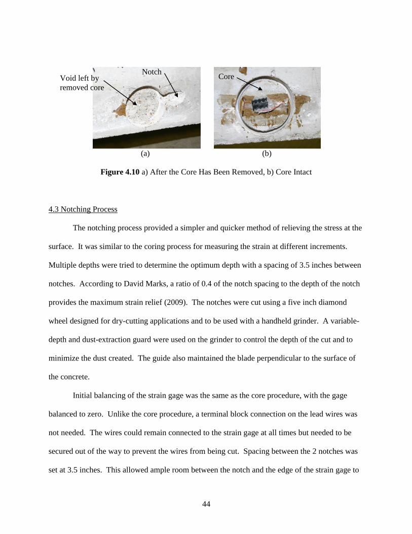
44
(a) (b)
Figure 4.10 a) After the Core Has Been Removed, b) Core Intact
4.3 Notching Process
The notching process provided a simpler and quicker method of relieving the stress at the
surface. It was similar to the coring process for measuring the strain at different increments.
Multiple depths were tried to determine the optimum depth with a spacing of 3.5 inches between
notches. According to David Marks, a ratio of 0.4 of the notch spacing to the depth of the notch
provides the maximum strain relief (2009). The notches were cut using a five inch diamond
wheel designed for dry-cutting applications and to be used with a handheld grinder. A variable-
depth and dust-extraction guard were used on the grinder to control the depth of the cut and to
minimize the dust created. The guide also maintained the blade perpendicular to the surface of
the concrete.
Initial balancing of the strain gage was the same as the core procedure, with the gage
balanced to zero. Unlike the core procedure, a terminal block connection on the lead wires was
not needed. The wires could remain connected to the strain gage at all times but needed to be
secured out of the way to prevent the wires from being cut. Spacing between the 2 notches was
set at 3.5 inches. This allowed ample room between the notch and the edge of the strain gage to
Notch Void left by
removed core
Core

45
prevent the possibility of the edge of the cut chipping out and damaging the gage. This spacing
was also used with the LSI device and a direct comparison was made between the two methods.
With the LSI device, initial readings had to be taken once mounting brackets and the surface
were prepared. A set of 10 reference readings were taken and an average of all 10 was used in
calculating the prestressing force. To ensure high-quality reference readings were taken, another
set of measurements was taken after the reference readings. To take the second set of readings,
the device was removed from the mounting brackets and then repositioned. Once repositioned,
another 10 measurements were taken. This ensured no false readings had been taken and the
device was working properly.
From the center of the gage, a line was drawn 1.75 inches from each side of the center
and 5 inches up. The line served as a reference for where to cut. Total length of the line was
five inches, which allowed for a full-depth cut three inches up from the bottom of the beam or
one inch past the center of the top strand. The total cut of five inches represented the curvature
of the blade and the intersection on the surface at a cut depth of one inch. For the first 2 sets of
notches, depths from ½ inch to 1.25 inches in ¼-inch increments were cut around a linear-
resistance strain gage, with measurements taken at each depth. For the rest of the notches,
depths of ¾, 1, and 1.25 inches were cut. Five minutes elapsed between each notch depth to
allow the gage to stabilize.
To investigate effects of temperature on the notching procedure, a noncontact
thermometer was used. With this, initial temperatures of the beam, location of the notches, and
ambient temperatures were measured. After the notching was complete, a maximum temperature
increase of five degrees Fahrenheit was observed. Within a few minutes, the temperature around
the notches was found to be in equilibrium with the surrounding beam. This temperature was

46
much lower than the coring temperature increase, and the temperature increase of five degrees
provided minimal strain drift.
4.4 Calculation of the Average Prestress Force
To find the average prestress force in the beam, the measured relaxation of strain had to
be converted to the change in stress, which was then related to the stress in the concrete. Using
the calculated modulus of elasticity, the strain relief was converted by equation 4.1, Hooke’s
Law, assuming the concrete is linear elastic.
(4.1)
where
σ = relieved stress (psi),
E = concrete modulus of elasticity (psi), and
ε = relieve strain (in/in).
The prestress force was then solved from the known stress by the following equation:
(4.2)
where
σ = relieved stress (psi),
P = prestress force (lbs),
A = cross sectional area (in2),
e = prestress force eccentricity (in),
y= distance from the neutral axis (in),

47
I = moment of inertia (in4), and
M = moment due to mass of beam (lb-in).
The moment was calculated from the mass of the beam, but if additional dead load was
on the beam at the time of testing such as a bridge deck or floor, the moment due to the dead load
would be taken into account within the moment term. The distance from the neutral axis was
measured as the distance from the neutral axis to the center of the strain gage. This was done to
relate the calculated prestress force to the measured strain at the location where the strain gage
was mounted.
4.5 Determining the Modulus of Elasticity of the Concrete
Two methods were used to determine the modulus of elasticity of the concrete—
calculating the modulus from the beam during the crack-open procedure, and in accordance with
ASTM C 469. Calculating the modulus from the crack-opening procedure will be discussed in
section 6.3.2, Analysis of Crack-Opening Data.
To determine the modulus of elasticity based on ASTM C 469, four-by-eight-inch
concrete cylinders were used from the casting of the beam. Multiple cylinders were made during
the casting of the beam to represent a sample of the beam to be used to test the compression and
modulus of the concrete. Each cylinder was cured in a similar method as the beam, to represent
the properties of the beam and not the ultimate strength of the concrete. The cylinders were
tested during the surface-strain relief method to determine the modulus of elasticity of the
concrete. The moduli of concrete changes as the strength of the concrete changes. Since the
beams were tested at approximately 28 days, after 6 months of curing, the modulus could vary
significantly. Two samples were tested for each beam, with each sample cycled three times.

48
The samples were tested using a servo-controlled hydraulic actuator to apply the load, and a
compressometer was used to measure the strain on the concrete. Using a 16-bit data acquisition
system, the load and displacement, measured by the compressometer, were sampled at 2 hertz.
The first cycle was not used in the calculation of the modulus due to possible errors in the
installation of the compressometer and of the compression caps used to even out any
irregularities, as well as to allow for the cylinder to be loaded uniformly. The chord modulus
was determined using the procedure in ASTM C 469 (2002).

49
Chapter 5 Finite Element Models
To visualize the stress distribution and test many different combinations of core depths
and notch configurations, finite element models were created using Abaqus CAE software. The
models represented the prestress members used for the laboratory experiments. Each model was
first created without a core but with similar dimensions and material properties. The models’
stress due to the applied prestressing force was then compared to the theoretical stress calculated
in the prestress member to determine if the model was built accurately. Finally, either a core or
two notches were added at the mid-span of the beam.
5.1 Rectangle Beam Models
Initially a base model was created with the same cross-sectional properties as the
laboratory specimens. The models did not include information on the transfer length, so high-
stress concentrations existed at each of the beams. For determining stresses on the model, the
midpoint of the beam was used, which did not include the stress concentrations due to the
disregard of the transfer length in the model.
5.1.1 Model Parameters
Each model started with the base model that consisted of a beam 6 inches wide by 12
inches deep, and a total length of 120 inches. Beams were restrained in the model similar to a
simply supported beam, as shown in figure 5.1, with one end pinned and the other end supported
on a roller. Two ½ inch strands were positioned in the bottom of the beam, represented as a
stringer, and an initial stress of 150 ksi was applied to each stringer representing the prestressing
force. An elastic modulus of 3,100 ksi for the concrete, with a Poisson’s ratio of 0.2 and 28,500
ksi for the prestress steel elastic modulus and a Poisson’s ratio of 0.3, were the only material
properties entered into Abaqus. Tensile and compressive strengths were not included into the

50
models due to the fact that no stress exceeded yield or fracture points, and it was assumed that all
materials behaved with linear elastically. The top bars were omitted from the model for
simplicity because they provided limited stiffness to the model. The top bars were placed in the
research specimens to limit the tensile stress in the top of the beam, to satisfy ACI requirements
and to prevent cracking of the top portion of the beam.
Figure 5.1 Finite Element Model Restraint
The mesh for each model consisted of beam elements for the prestressed strand and
structural hex elements for the rest of the model. Partitions were created around the core or
notch to create a finer mesh in this area of interest at the mid-span. This refinement was used
also to reduce the computational time of each model. Each model had approximately 8,000
elements, with the finer mesh having an approximate element size of ¼ inch and the rest of the
model having an approximate mesh size of 1 inch.
Multiple models were created using the base model, with varying depths of cores and
notches. The first three models had cores in the side of the beam with three varying depths—¾,
1, and 1.25 inches. The cores were represented by removing the material between the inner and
Pin Support
Roller Support

51
outer diameter of the core bit, leaving a cylindrical ring cut out. A spacing of 3.5 inches was set
as the distance between the notches. Marks determined that a ratio of depth versus the spacing of
the notches to be 0.4 (2009), so this was used as a starting point for the first model. The first
model created had a notch depth of 1.25 inches with spacing between notches of 3.5 inches. The
notch was modeled as a cut three inches long at the bottom of the notch, creating the total length
on the surface to be approximately five inches. This model seemed to overestimate the residual
stress in the member and a significant tensile stress was seen on the surface. The depth of the
core was reduced to one inch, with everything else staying the same, and full relaxation was not
achieved. The depth was then increased to 1.125 inches and a full relaxation was shown with no
significant tensile stresses present. For the prestress beams, a ratio of depth versus spacing of
0.33 results in full relaxation. To test this hypothesis, the depth was changed to one inch and the
space was reduced to three inches, which resulted in a similar full relaxation. Total length of the
notch was also varied but was not found to affect the results significantly.
5.1.2 Results
All models started from the same base model and contained the same parameters. Thus
they could be compared directly to one another. To compare the models, stresses were measured
at each node location along the center of the core or notch as shown in figure 5.2, showing the
stress distribution. This area along the center of the core or notch would also be where the strain
measurement would be taken with a strain gage or LSI device. To determine the residual stress
that would be measured by a strain gage or the LSI device, the stress values were plotted as in
figure 5.3, and Simpson’s rule was used to calculate the area under the curve where the strain
gage would be positioned. Stress near the edges was near zero as expected, but a tensile stress

52
increase followed with a decrease in stress to the midpoint. To get a full relaxation, the tensile
stress needed to be balanced out by the compressive stress towards the midpoint of the core.
(a)
(b)
Figure 5.2 (a) Stress Distribution across Core, (b) Stress Distribution across Notch

53
Figure 5.3 Plot of Stress along Length of Strain Gage
Table 5.1 shows the depth of the core and the calculated stress using Simpson’s Rule,
along with the percent of relieved stress. The percent of relieved stress was calculated from the
prestressing stress of 1490 psi, which was found on the non-cored beam 2 inches up at mid-span
of the beam. Both table 5.1 and figure 5.4 show that ¾ inch core depth does not provide a full
relaxation of the stress and that the 1.25 inch core depth provides a full relaxation. But some
induced bending stresses resulted causing a tensile stress, which over-predicts the amount of
applied prestress force. The 1 inch core depth balanced out the compressive stresses and tensile
stresses, providing a near 100% relief of stress, just slightly overestimating the prestressing
stress.

54
Table 5.1 Calculated Stresses and Percent Relieved across Cores
Figure 5.4 Plot of Stress on Surface of Cores
Stresses relieved by the notches were more dependent on depth than on the cores. Figure
5.5 shows the plots of the varying depths of notches, while keeping the spacing and length of the
notch constant. A depth of 1.125 inches was found to represent a full stress relief as seen in table
5.2. A change in depth of ± 0.125 inch results in a large change in relieved stresses, either
under- or over-estimating the residual stresses.
Core Depth (in)Simpson's Rule
Calculated Stress (psi)
% Relieved
Stress
0.75 -266 82%
1.00 15 101%
1.25 174 112%

55
Figure 5.5 Plot of Stress between Notches
Table 5.2 Calculated Stresses at a Spacing of 3.5 in, Length of 3 in, and Varying Depth
There are more variables to the notching procedure to relieve the stress than just the
depth of the notch. To look at these, three models were created to examine the spacing of the
notches and three models to view the length of the notches. The three models varied the total
length of the notch that was cut to the full depth of one inch. The lengths looked at were 2
inches, which is up to the strand height, 3 and 4 inches, while keeping the spacing at 3.5 inches
and a depth of 1 inch. Figure 5.6 shows lengths of 2 and 3 inches are very similar, with a length
Notch Depth (in)Simpson's Rule
Calculated Stress (psi)
% Relieved
Stress
1.00 -352.85 76%
1.13 3.97 100%
1.25 317.93 121%

56
of 4 inches relieving the least amount of stress. Table 5.3 reinforces that the relief of stress
between a length of 2 and 3 inches is similar at 76% but still not full relaxation. Next, the
spacing between the notches was modified to see its effects on the relieved stress. Three spaces
of 2.5, 3, and 3.5 inches were compared using a constant depth of 1 inch and a length of 3 inches.
Figure 5.7 shows the plots of the three varying lengths, with each spacing aligned with the center
of the others. As the spacing got closer together, the amount of relieved stress increased. At a
spacing of 2.5 inches, influences of each notch seemed to influence the relieved stress, creating a
positive tensile residual stress between the notches. Table 5.4 shows the calculated stresses and
the percent of relieved stresses. A spacing of 3 inches seems acceptable, with a 5% error.
Figure 5.6 Plot of Varying Length of Notches

57
Table 5.3 Calculated Stresses at a Notch Depth 1 in, Spacing of 3.5 in, and Varying Length
Figure 5.7 Plot of Varying the Spacing of Notches
Table 5.4 Calculated Stresses at a Depth of 1 in, Length of 3 in, and Various Spaces
Notch Length (in)Simpson's Rule
Calculated Stress (psi)
% Relieved
Stress
2.00 -351.47 76%
3.00 -352.85 76%
4.00 -689.35 54%
Notch Spacing (in)Simpson's Rule
Calculated Stress (psi)
% Relieved
Stress
2.50 283.18 119%
3.00 81.45 105%
3.50 -352.85 76%

58
According to Marks, the ratio of depth to spacing should be around 0.4 (2009). The 2
combinations of notches seem to be a depth of 1 inch and a spacing of 3 inches, or a depth of
1.125 inches and a spacing of 3.5 inches, each having a ratio of approximately 0.33. For the
surface-strain relief method, a spacing of 3.5 inches was chosen to allow ample space around the
strain gage and to allow for use of the LSI device, which had a larger gage length.
5.2 T-beam Models
T-beam models were made to represent the T-beams’ specimens tested with the surface-
strain relief method. The models looked at the core depth and notch depth found from the
rectangle beam models. These models were similar to the rectangle beams, not including
transfer length or shear reinforcement placed in the member.
5.2.1 Model Parameters
The models had the same cross-section properties as the T-beam described in section 3.3.
Simply supported beam restraints were applied with a pin end on one end and a roller support on
the other. Each T-beam had two 3/8 inch strands represented by stringers with equal area to a
3/8 inch prestressing strand, and an initial stress of 150 ksi was applied to each stringer.
Concrete and prestressing steel properties remained the same as the rectangle beams, due to
limited information on the properties of the beams at the time of creating the models. The T-
beam was partitioned to have a finer mesh around the notches and core with an approximate size
of ¼ inch, with an approximate mesh size of 1 inch for the rest of the model. Each model
contained around 64,000 elements, which consisted of beam elements representing the
prestressing steel and structural hex sweep elements for the concrete T-beam. An initial model
was created and then three different models were made, one to represent a core perpendicular to
the surface of the beam at a depth of 1 inch, a core that was parallel to the bottom surface with a

59
depth of 1 inch at the bottom of the core, and a final model consisting of 2 notches 1.125 inches
in depth. Figure 5.8 shows a cross-section of the T-beam with either a notch or core cut into the
side and the dimensions.
(a) (b)
(c)
Figure 5.8 a) Core Parallel to Bottom of Beam, b) Core Perpendicular to Web, c) Notch
5.2.2 Results
From results of the finite element models of the T-beams, it can be seen that optimal
depths and notch configurations determined from the other finite element models will also apply

60
to the T-beam and provide an acceptable relief stresses. Table 5.5 shows the stresses that remain
on the surface of the core or notch, and what percentage of stress is relieved compared to the
applied prestressing force. Two core models compared effects of the direction of the core, one
core being parallel to the base of the beam or perpendicular to the prestressing plane, and the
second core perpendicular to the web of the beam. The core parallel to the bottom of the beam
showed that 103% of the stress had been relieved, which was very close to the rectangle beam
model of a core to a depth of 1 inch. The core parallel to the base had a complete relief of stress
and introduced some bending stress into the surface of the core. The core perpendicular to the
web had a similar relief of stress as the parallel core, as shown in figure 5.9, showing that the
direction of the core is not as important as the depth of the core. The notch model provided
similar results as the other models, with slight over-prediction of the relieved stress. In order to
create one method acceptable to all shapes and configurations, the depths and notch
configurations developed for the rectangle beams are within 10% of the full relaxation on the
surface of the T-beam.
Table 5.5 T-Beam Calculated Stresses
MethodSimpson's Rule
Calculated Stress (psi)
% Relieved
Stress
Core Parallel 20.53 103%
Core Perpendicular -23.22 97%
Notch 64.85 109%

61
Figure 5.9 Surface Stress Comparing Direction of Core

62
Chapter 6 Determining the Average Prestress Force
The surface-strain relief method calculates average prestress force from the change in
surface strain. To determine accuracy of the method, average prestress force must be known.
Multiple methods were used to calculate average prestress force, including calculation of losses,
measuring losses, and a crack-opening procedure. First a series of calculations were used to
estimate prestress losses based on the PCI Design Handbook and ACI 318-08. Calculation of
losses is a conservative estimate and serves as a reference to determine an approximate prestress
force after losses. To get an accurate measurement, average prestress force was calculated from
experimental results, using a method similar to a method used by Larson, Peterman, and Rasheed
(2005) and also by Pessiki, Kaczinski, and Wescott (1996). Losses were also measured through
use of a Whittemore gage at the mid-span of the beams cast at KSU. This was determined to be
the most accurate way to measure losses of the rectangle beams.
6.1 ACI Loss Calculations
The purpose of this research project was not to measure the losses of prestress members
but to determine the remaining prestress force in a member for comparison purposes to the
method of surface-strain relief. Losses were calculated based on ACI 318-08 and the PCI
Handbook only to serve as a check that average prestress force (fse) calculated from experimental
procedures was in the expected ranged based on the expected losses. Losses due to creep,
shrinkage, relaxation of the tendons, and elastic shorting were all considered and individual
losses for each beam were calculated. Effective stress in the prestressing steel after losses for the
first set of beams was 130 ksi and for the second set was 122 ksi. The T-beam average
prestressing stress after losses was determined to be 167 ksi.

63
6.2 Use of Whittemore Gage to Determine Losses
To measure the losses of the beam, a Whittemore gage was used. The gage measures the
deviation between two points from its set gage length of eight inches. The deviation distance is
measured by a dial gage with an accuracy of 0.0001 inch. For the rectangle beams cast at K-
State, two brass points were cast into the side of each beam eight inches apart. Initial
measurements were taken before de-tensioning the beam and once again immediately after de-
tensioning. Comparing the initial measurement to the de-tensioning measurement, the initial
losses can be calculated by computing the change in length between the two measurements and
dividing by the gage length to convert to a strain. Due to the nature of concrete, the modulus of
elasticity is not linear during the curing process; therefore the strain measured by the Whittemore
gage is compared to the relaxation of the strand which has a constant modulus of elasticity up to
the point of yield. The prestressing steel was tensioned to 75% of the ultimate strength,
therefore, the prestressing steel can be assumed to have a constant modulus. To determine the
long-term losses and total losses at the time of testing the surface-strain relief method,
measurements were taken before coring to calculate the losses at the time of coring.
The surface-strain relief method calculates the prestressing force and not the losses. So
in order to calculate prestressing force, initial stresses of each strand were needed. Load cells
were positioned on each strand throughout the casting process to measure the stresses in each
strand. Before de-tensioning, the load in each strand was recorded and assumed as the initial
force in each strand. Losses measured from the Whittemore gage were then subtracted from this
initial stress in the strand. For the beams cast in the laboratory, this was assumed to be the most
accurate method of determining average prestressing force in each beam and was used as a bench
mark when determining the accuracy of the crack-opening method.

64
6.3 Crack-Opening Method to Determine the Average Prestress Force
To accurately calculate fse of each beam tested using the surface-strain relief method, a
combination of procedures used by Larson, Peterman, and Rasheed (2005), and Pessiki,
Kaczinski, and Wescott (1996) was used. Each beam was initially loaded past the calculated
mid-span cracking moment, instrumented with displacement transducers, and then loaded past
the cracking moment for an additional 25 cycles. Unlike the two methods researched, the
displacement transducers were positioned at the height of the strand and mounted on the side of
the beam. This allowed the crack width to be measured at the level of the strand rather than the
base of the beam. With the displacement transducers mounted on the side, the force required to
open the crack and produce zero concrete tension near the strand could be found.
6.3.1 Crack-Opening Method Setup
The beams were loaded in a three-point bending setup using a hydraulic servo-controlled
actuator (see figure 6.1). At each end of the beam, a steel-bearing plate was positioned on a
concrete-bearing block and one was positioned on the bottom side of the beam using a high-
strength gypsum cement to fill in any voids between the bearing plate and the concrete surface.
Between the two bearing plates, a 1.5 inch roller was used to prevent the horizontal restraint at
the beams ends. At mid-span, a four-inch-wide bearing plate was attached to the top surface of
the beam using high-strength gypsum cement to fill in the voids on the rough concrete surface.
A one inch steel roller was positioned between the bearing plate and the hydraulic actuator. Two
LVDTs were positioned at the mid-span, mounted above the beam, and attached to the top
bearing plate to measure the deflection of the beam, as shown in figure 6.2. Two additional ½
inch LVDTs were mounted on the side of beam (see figure 6.3) at mid-span using the 3/8 inch
bolts cast into the beam to measure the crack width. Each beam was initially loaded to 40% past

65
the calculated cracking moment to create a visible crack. The load was held for 1 minute to
mark the location of the crack, and the beam was unloaded to 100 lbs. The beam was then
loaded to the same maximum applied load as initially, at a rate of 3500 lbs/min, and unloaded at
the same rate for a total of 25 cycles. For the rectangle beams, each was loaded to the maximum
applied load of 14,000 lbs and the T-beam was loaded to 9000 lbs. Deflection, load, actuator
displacement, crack width, and time data were collected at two hertz throughout all cycles.
Figure 6.1 Beam Setup
Hydraulic Actuator
Roller Support

66
Figure 6.2 Deflection Measurement Setup
Figure 6.3 LVDT Mounted to Measure Crack Width
6.3.2 Analysis of Crack-Opening Data
Data from each beam was separated into individual cycles so the cracking moment for
each cycle could be found. From the data, the modulus of elasticity was calculated using load
10” LVDT
Bearing Plates

67
versus deflection for relating relief strains to stresses. To find the crack opening or
decompression load, multiple methods were analyzed including the end of linearity and a double
line method. The double-line method takes into consideration the bilinear response of the load
versus crack opening.
Using the initial loading, which cracked the beam, and the first cycle data, the modulus of
elasticity was calculated using the applied load and mid-span deflection. The data was examined
up to 50% of the cracking moment to insure the crack had not yet formed, which would reduce
the cross section and would create a crack section and a varying moment of inertia. Assuming
the load is applied similar to a point load, the modulus of elasticity can be found by solving for
the modulus of elasticity in the following equation for the deflection of a simply supported beam:
where,
δ = mid-span deflection (in),
P = applied load (lbs),
L = clear span between supports (in),
E = modulus of elasticity (ksi), and
I = moment of inertia (in4).
Using the average measured deflection and the applied load, the modulus of elasticity
was solved for each load and averaged throughout the cycle to find the modulus of the beam.
Initial loading and the first cycle were used because once the beam has been repeatedly cracked
it loses some stiffness, resulting in a smaller modulus of elasticity. When using the applied load
(6.1)

68
and deflection to find the modulus of elasticity, the modulus of the entire beam is found and not
the modulus of the concrete.The cyclic loading on the beam thus reduces the overall stiffness of
the beam resulting in a lower measured beam modulus of elasticity. The initial loading of the
beam had not been cracked, so the beam can be considered a representation for the concrete
modulus of elasticity. The modulus was calculated to be used in conjunction with the surface-
strain relief method, to relate the measured strain to the residual stress.
The data, applied load versus the crack width, was plotted for each cycle, and a bilinear
response was seen, as in figure 6.4. To calculate the average prestress force, the cycles were
each evaluated using two methods—looking at both the bilinear response and at the end of
linearity. The double-line method uses the bilinear response to fit two linear regression lines
before the crack opens, and then after the crack is fully open. The point where these two lines
cross is equal to the load that is required to first open the crack. Pessiki, Kaczinski, and Wescott
used this method to determine the decompression load when strain gages were used as the
displacement measurement device. The decompression results were found to be repeatable and
vary no more than 3 to 5% (1996).

69
Figure 6.4 Graph of Bilinear Response
Two bilinear portions of the graph were looked at—0 to 7,000 lbs and 11,000 to 14,000
lbs for the rectangle beams, and 0 to 3,000 lbs and 5,000 to 9,000 lbs for the T-beams. The
initial portion of the graph was linear up until the crack opened, and the second portion was
linear once that crack was fully opened. To fit a line of best fit to these linear portions, the slope
and the y-intercept were calculated using the following linear regression equations:
∑( ) ∑ ∑
∑( ) (∑ )
(6.2)
∑ ∑
(6.3)

70
where,
m = slope of the line,
b = y-intercept,
n = number of data elements considered,
x = crack width data, and
y = applied load data.
Figure 6.5 shows the plot of each linear line and the point of intersection, which was
examined to be the point of the decompression load. To ensure the portions were linear, the
correlation coefficient was calculated for each portion.
Figure 6.5 Linear Regression Lines Plotted on Graph

71
The next method was to determine the end of linearity; the same procedure was followed
to create the linear regression line from 0 to 7,000 lbs for the rectangle beams and from 0 to
3,000 lbs for the T-beams. Using the equation of the regression line, a predicted crack width was
calculated based on the applied load. To determine the end of linearity, multiple methods were
evaluated. One way was to determine a range when the end of linearity occurred. A visible
inspection was used to give a rough value of where the end of linearity occurred. The second
method looked at the amount of deviation between the predicted crack width based on the
regression line and the actual measured crack width. The point when the predicted crack width
differed from the actual crack width by more than 0.0002 inches was considered to be the end of
linearity. This difference was well within the resolution of the 16-bit data acquisition system and
the ¼ inch LVDT that was measuring the crack width.
Both methods showed similar decompression loads for all cycles, with the maximum
decompression load occurring on the 1st cycle and the least decompression load occurring on the
25th
cycle. The decrease in load can be attributed to the bond being broken around the strand at
the location of the crack. With the bond broken, the friction between the strand and the concrete
was reduced; therefore, requiring less force to open the crack. Following Larson, cycles 1
through 10 were considered for determining the crack-opening moment (2002). Table 6.1 shows
the decompression loads for both the double-line method and the end of linearity with the first 10
cycles recorded, and then every 5 cycles after that. After the tenth cycle, minimal change can be
seen in the applied load required to open the crack. Once all the data were plotted, the load at the
intersection point was recorded along with the load at which the end of linearity occurs. Once all
the data were analyzed, the extreme values were excluded and an average applied load was

72
determined. An average load was determined for each method and then the average prestressing
force was calculated.
Table 6.1 Applied Loads to Open Crack
To calculate average prestress force for each beam, the cracking moment was first calculated
from the average applied load, which resulted in zero concrete tension across the crack. Average
prestress force was calculated from the cracking moment of each beam as follows, by solving for
the average prestress force:
[
]
(6.4)
where,
CycleDouble Line
Method
End of
Linearity
1 10000 9200
2 10000 9000
3 10000 9000
4 9800 8800
5 9800 8750
6 9800 8700
7 9750 8650
8 9700 8650
9 9650 8600
10 9650 8600
15 9600 8600
20 9500 8600
25 9500 8550
Average 9729 8535
Applied Load (lbs)

73
MCR = cracking moment (lb –in),
I = section moment of inertia (in4),
P = average prestress force (lbs),
A = area of concrete (in2),
y = distance from neutral axis (in),
e = eccentricity (in), and
fr = modulus of rupture (psi).
The LVDT measured the width of the crack two inches from the bottom of the beam, or
at the height of the strand, so once the crack started to open at the LVDT, a crack was already
present from the bottom of the beam. To account for this crack, cracked transformed section
properties were used. The modulus of rupture was assumed to be zero since a crack former was
embedded at mid-span in each beam and prevented the transfer of any tensile stress in the
concrete. Once the average prestress force was calculated, the fse was calculated, to be compared
to the other methods that were used to find fse.
6.4 Results
Data gathered from measuring the losses using the Whittemore gage employed the most
direct method to determine fse in each of the rectangle beams. Average prestress stress measured
from the Whittemore gage can be found in table 6.2. Beams 1 and 2 were cast in series along
with beams 3 and 4, which show similar values when compared to each other. These values
were used as a benchmark to determine the accuracy of the crack-opening procedure, and to
determine a method to increase the accuracy of the method so fse could be found for the T-beams.
Table 6.3 shows the results from finding fse based on the two different methods, the double-line

74
method and the end of linearity for the first 10 cycles of beam 2. For the other three beams, table
6.4 summarizes fse for each method.
Table 6.2 fse Based on Losses
Table 6.3 Results of Crack-Opening Procedure for Beam 2
Beam fse (ksi)
1a 134.8
1b 135.0
2a 114.5
2b 98.0
Cycle Pco-End* (lbs) ML (k-in) Pe (lbs) fse (ksi) Pco-End* (lbs) ML (k-in) Pe (lbs) fse (ksi)
1 9200 276.0 41084 134.3 10000 300.0 44657 145.9
2 9000 270.0 40191 131.3 10000 300.0 44657 145.9
3 9000 270.0 40191 131.3 10000 300.0 44657 145.9
4 8800 264.0 39298 128.4 9800 294.0 43764 143.0
5 8750 262.5 39075 127.7 9800 294.0 43764 143.0
6 8700 261.0 38851 127.0 9800 294.0 43764 143.0
7 8650 259.5 38628 126.2 9750 292.5 43540 142.3
8 8650 259.5 38628 126.2 9700 291.0 43317 141.6
9 8600 258.0 38405 125.5 9650 289.5 43094 140.8
10 8600 258.0 38405 125.5 9650 289.5 43094 140.8
Average 8750 262.5 39075 127.7 9794 293.8 43739 142.9
*Pco-End = Appl ied load to ini tiate a crack
End of Linearity Method Double Line Method

75
Table 6.4 Summary of Crack-Opening Procedure
To compare all the methods, table 6.5 was created. Beams 1a and 1b were cast together
along with beams 2a and 2b. Beams 1a and 1b were almost identical in terms of fse, whereas
beams 2a and 2b showed some differences. The specific reason for the discrepancy was not
determined, however, it was determined that it was not due to the measurement of losses as all
methods showed this discrepancy. The measured losses were within the ACI calculated losses,
providing confidence that the measured losses were accurate. All beams tested were within 4%
of the calculated losses, except beam 2b where the measured losses were significantly lower than
the calculated losses. When looking at the crack-opening procedure methods—the end of
linearity and the double-line method—the end of linearity was within 6% and usually under-
predicted, with beam 1a being the only beam that calculated a greater stress than the measured
losses. The double-line method consistently found fse to be greater than the actual stress by an
average of 15%.
Beam Pco-End* (lbs) ML (k-in) fse (ksi) Pco-End* (lbs) ML (k-in) fse (ksi)
1a 9150 274.5 135.4 10300 309.0 152.0
1b 8750 262.5 127.7 9800 294.0 142.9
2a 7600 228.0 111.6 9200 276.0 133.8
2b 6200 186.0 92.6 8250 247.5 120.7
*Pco-End = Appl ied load to ini tiate a crack
Average of End of Linearity
MethodAverage Double Line Method

76
Table 6.5 Summary of All Stress Determination Methods
The end of linearity served as reasonable method to determine fse from the crack-opening
procedure. This method would be used on the T-beams to determine the average prestressing
force in the two beams tested. Table 6.6 shows fse from the calculated losses based on ACI for
each T-beam, and based on the end of linearity and the crack-opening procedure. A larger error
is shown between the losses and the crack-opening procedure, but the calculated losses were
calculated based off of limited information, the age of the beams was approximately nine years
old, and information was not available about whether the beams had been damaged or tested
before.
Table 6.6 T-Beam Calculated fse
Beam Measured Losses ACI Calculated Losses End of Linearity Double Line
1a 134.8 130.0 135.4 152.0
1b 135.0 130.0 127.7 142.9
2a 114.5 117.0 111.6 133.8
2b 98.0 117.0 92.6 120.7
1a 3.6% -0.4% -12.8%
1b 3.7% 5.4% -5.9%
2a -2.2% 2.5% -16.9%
2b -19.4% 5.5% -23.2%
Calculated f se base on (ksi):
Percent Error Based on Measured Losses
T-beam ACI Calculaated Losses End of Linearity
1 165 129.3
2 165 146
Calculated f se base on (ksi):

77
Chapter 7 Surface-Strain Relief Method Results
Multiple methods were tried on different beams and were related to the calculated
average prestress force determined from the measured losses and the crack-opening procedure.
Factors influencing the residual stress were also monitored, such as the increase of temperature
due to coring, determining the modulus of elasticity, and depth of the notches and core. The
results were also compared to the finite element models to determine if the models represented
the specimens so that different beams could easily be modeled to determine the optimum core
depth or notch configuration.
7.1 Modulus of Elasticity of the Concrete Beams
The modulus of elasticity calculated from the ASTM C 469 specification was used in all
calculations to determine average prestressing force from the method of surface-strain relief with
the rectangle beams. Following ASTM C 469 (2002), the modulus of the concrete was found
and not the modulus of the entire beam. The modulus determined from the load versus
deflection curve showed a lower modulus than ASTM C 469. Determining the modulus from a
cylinder is much more feasible, and for a prestress member, the ability to obtain a core from the
member would be simpler than loading the member and measuring the deflection over varying
loads. For the surface-strain method to be feasible, not only must the method be feasible, but
also the method of determining the modulus of elasticity. For an existing structure, the modulus
could be determined from a core sample, which would follow the ASTM specification giving
similar results to the research conducted for this phase. For the T-beams, the only modulus
determined was from the crack-opening procedure. The web of the member was too narrow,
along with the mesh reinforcement providing difficulty in obtaining a sample. With the
calculated modulus of elasticity from ASTM and the load versus deflection on the rectangle

78
beams, a high level of confidence was found between the two methods. Table 7.1 shows the
modulus determined following ASTM and from the load versus deflection. When comparing the
ASTM E-chord method and the load versus deflection method, a maximum difference of 300 ksi
is seen. ASTM standard rounds the calculated modulus of elasticity to the nearest 50 ksi, so a
variance of 300 ksi is fairly insignificant.
Table 7.1 Modulus of Elasticity
7.2 Rectangle Beam Results
To compare multiple methods of coring, notching, and measuring strain, multiple
methods were used on each beam. The first set of beams tested, which included beams 1a and
2a, were initially tested with the method of coring around a strain gage. Each beam had multiple
cores and/or notches made at different locations along both sides of the beam. Each location was
offset from the location on the opposite of the beam so two test locations would not line up,
which would reduce the cross-sectional area at that location. A reduced cross-sectional area
would result in an increase in measured strain and affect the accuracy of the measurement.
Beam 1a only used the coring method and was tested three months after the beam was cast.
Beams 1b, 2a, and 2b used a combination of both methods, cores and notches, and also used both
BeamE-Chord
Method
Load versus
Deflection
1a 3750 3500
1b 3300 3000
2a 3950 3800
2b 3550 3350
T-beam 1 - 3550
T-beam 2 - 3000
Modulus of Elasticity (ksi)

79
strain gages and the LSI device. Beam 2a was tested one month after casting, while beams 1b
and 2b were tested about 10 months after the beams were cast. Overall, the cores showed a
larger release of strain without measuring a tensile stress across the core, which over calculates
the amount of prestressing force in the beam.
7.2.1 Core Results
The first beam cored was beam 1a, and four gages were successfully cored. Due to tight
tolerances between the strain gage and edge of the core, one gage was damaged while coring and
another gage experienced substantial drift during the process. Table 7.2 shows the measured
strains on beam 1a at a 0.75 inch depth and 1 inch depth, along with the percent error when
compared to the theoretical strain measurement calculated from the measured losses and the
experimental decompression load. The cores were taken at various locations along each side of
the beam. The surface-strain relief method gave consistent results on beam 1a at the varying
depths, as with the other beams. Two cores were cored in the side of beam 1b and showed
similar results as with beam 1a; the remaining locations on the beam were used to test other
methods of relieving strain. Table 7.3 shows the relieved strain at a depth of 0.75 inch and 1
inch for beam 1b.
Table 7.2 Measured Strains on Beam 1a Using the Coring Procedure
Core Theoretical (με) 3/4" Depth (με) 3/4" Percent Error 1" Depth (με) 1" Percent Error
1 330 301 8.8% 314 4.8%
2 331 298 10.0% 328 0.9%
3 329 325 1.2% 361 -9.7%
4 331 297 10.3% 332 -0.3%

80
Table 7.3 Measured Strains on Beam 1b Using the Coring Procedure
The next set of beams, 2a and 2b, had similar amounts of cores taken out of each. The
first beam in the set cored was beam 2a and it had three cores tested on one side and two on the
other. Table 7.4 shows results from the coring procedure. Similar results were found when
compared to the first set of beams cored. Four cores were taken from beam 2b, as shown in table
7.5, with the second core being damaged during the incremental depth increase from 0.75 to 1
inch.
Table 7.4 Measured Strains on Beam 2a Using the Core Procedure
Table 7.5 Measured Strains on Beam 2b Using the Core Procedure
Core Theoretical (με) 3/4" Depth (με) 3/4" Percent Error 1" Depth (με) 1" Percent Error
1 381 279 26.8% 351 7.9%
2 381 309 18.9% 390 -2.4%
Core Theoretical (με) 3/4" Depth (με) 3/4" Percent Error 1" Depth (με) 1" Percent Error
1 269 240 10.8% 290 -7.8%
2 268 220 17.9% 254 5.2%
3 268 250 6.7% 300 -11.9%
4 268 261 2.6% 290 -8.2%
5 269 224 16.7% 247 8.2%
Core Theoretical (με) 3/4" Depth (με) 3/4" Percent Error 1" Depth (με) 1" Percent Error
1 266 184 30.8% 235 11.7%
2 268 236 11.9% - -
3 266 197 25.9% 219 17.7%
4 268 273 -1.9% 278 -3.7%

81
As shown tables 7.4 and 7.5, the measured strains were all consistent with the theoretical
strains. Next, relieved strains were used to find the average prestress force at each core location,
and then an average was taken for each beam. Average prestress force calculated from the
surface-strain relief method was then compared to the average prestress force determined from
the measurement of losses and or the decompression load. Table 7.6 shows results of the coring
method on all four beams. At a core depth of 0.75 inch, larger errors are present and vary from
7% to 24%. At a core depth of 1 inch, much less error occurs with all the beams having an error
of less than 10% when compared to the experimentally determined fse.
Table 7.6 Calculated fse and Percent Error for the Core Method
Beams 1a and 1b were cast together in the same prestressing bed, along with beams 2a
and 2b. Theoretically beams 1a and 1b, and 2a and 2b should have the same average
prestressing force, so by testing one beam within the first three months after casting, and then
testing the second beam at a minimum of six months after casting, the effects of creep and
shrinkage on the relieved strain could be examined. When comparing beams 1a and 1b and
beams 2a and 2b, the average error varies from initially measuring a larger relief strain to
measuring less than a full relief. Beams 1b and 2b show a larger error than beams 1a and 2a,
suggesting that some time-dependent losses such as creep and shrinkage of the concrete may not
be easily measured using the surface-strain relief method.
BeamExperimentally
Determined f se (ksi)
3/4" Core Depth
Calculated f se (ksi)
Percent
Error
1" Core Depth
Calculated f se (ksi)
Percent
Error
1a 134.8 125.1 7.2% 136.4 -1.2%
1b 135.0 103.2 23.6% 128.9 4.5%
2a 114.0 101 11.4% 116.4 -2.1%
2b 98.0 83.1 15.2% 90.4 7.8%

82
7.2.2 Notch Results
Beams 1b, 2a, and 2b tested the method of the notching procedure to compare the results
to the finite element models and compare the LSI device to the linear electrical-resistance strain
gage. Beams 1b and 2b tested both the LSI device and strain gages on each beam, and the results
are shown in tables 7.7 and 7.8. Results for both methods are much more varied than the core
method. When comparing the strain gage to the LSI device, the LSI device provided more
accurate results. One explanation for this is that the LSI device measured over a larger surface
and measured close to the edge of the notch, which captured both tensile and compressive
stresses between the notches, as seen with the finite element models. The strain gage had a
smaller gage length and did not capture the strain over the entire surface. Beam 2a only used the
LSI device to measure the strain relief from the notching procedure, as shown in table 7.9.
Overall, the LSI device showed that 1.25 inches generally measures a resultant tensile strain on
average 20% larger than the theoretical strain. The 1-inch-depth errors were much closer to a
full relaxation, with errors around 10 to 15% less than the actual prestress force.
Table 7.7 Measured Strains on Beam 1b Using the Notch Procedure
Notch Theoretical (με) 1" Depth (με) 1" Percent Error 1.25" Depth (με) 1.25" Percent Error
1 383 236 38.4% 323 15.7%
2 383 200 47.8% 248 35.2%
*3 382 310 18.8% 369 3.4%
*4 384 293 23.7% 311 19.0%
* Used LSI device to measure strain

83
Table 7.8 Measured Strains on Beam 2b Using the Notch Procedure
Table 7.9 Measured Strains on Beam 2a Using the Notch Procedure
To calculate the average error for the strain gage and the LSI device, at the two depths of
1 inch and 1.25 inches, each notch location of the average prestress force was calculated and
compared to the experimental prestress force as shown in table 7.10. Results varied from beam
to beam, but overall the strain gages had larger errors at the depth of 1 inch and 1.25 inches when
compared to the results obtained from the LSI device.
Table 7.10 Calculated fse and Percent Error for the Notching Method
Notch Theoretical (με) 1" Depth (με) 1" Percent Error 1.25" Depth (με) 1.25" Percent Error
1 266 283 -6.4% 305 -14.7%
2 266 327 -22.9% 352 -32.3%
*3 268 240 10.4% 302 -12.7%
* Used LSI device to measure strain
Notch Theoretical (με) 1" Depth (με) 1" Percent Error 1.25" Depth (με) 1.25" Percent Error
*1 268 288 -7.5% 316 -17.9%
*2 268 303 -13.1% 323 -20.5%
* Used LSI device to measure strain
BeamExperimentally
Determined fse (ksi)
1" Notch Depth
Calculated fse (ksi)
Percent
Error
1.25" Notch Depth
Calculated fse (ksi)
Percent
Error
1b 134.8 79.2 41.2% 101.8 24.5%
*1b 134.8 107.6 20.2% 120.6 10.5%
*2a 114.0 125.6 -10.2% 135.4 -18.8%
2b 98.0 106.4 -8.6% 119.1 -21.5%
*2b 98.0 89.8 8.4% 109.7 -11.9%
*Used LSI device to measure strain

84
7.3 T-Beam Results
Two T-beams were tested, T-beam 1 and 2, and were approximately nine years old at the
time of testing. Similar to the rectangle beams tested, the initial beam (T-beam 1) was tested
using the coring method. With T-beam 2, both methods were used, coring and notching. T-
beam 1 was successfully cored at 4 various locations, however, at 2 locations the gages were
damaged while trying to core around them due to the tapered web, causing the core bit to shift
and tear the edge of the strain gage. T-beam 2 successfully cored around four strain gages and
tested the notching procedure at five locations. As with the rectangle beams, the cores provided
more precise and accurate results on the T-beams.
7.3.1 Core Results
Tables 7.11 and 7.12 show results of each core and incremental depth. A depth of 0.75
inches shows a full relaxation of the core is not achieved, but at a depth of 1 inch, the error is less
than 10%. On T-beam 2, larger errors existed on cores 3 and 4, showing errors of 50% at a depth
of 1 inch. No other core showed this kind of error, so each core was broken out to investigate the
reason behind the error and to see if any reinforcement was running through the core.
Reinforcement was found running through the core at a depth of 1 inch from the surface of the
web. The reinforcement ran vertically through the core as shown in figure 7.1. It was concluded
that the presence of the reinforcement significantly affected the relief of strain on the surface of
the member. The reinforcement allowed for less than 50% of the strain relief, so neither of these
cores was considered in the calculations of the prestressing force as shown in table 7.13.

85
Table 7.11 Measured Strains on T-Beam 1 Using the Coring Procedure
Table 7.12 Measured Strains on T-Beam 2 Using the Coring Procedure
Figure 7.1 Reinforcement Affecting Strain Relief on the Surface of the Core
Core Theoretical (με) 3/4" Depth (με) 3/4" Percent Error 1" Depth (με) 1" Percent Error
1 118 104 11.9% 123 -4.2%
2 118 101 14.4% 126 -6.8%
3 122 103 15.6% 108 11.5%
4 118 111 5.9% 113 4.2%
Core Theoretical (με) 3/4" Depth (με) 3/4" Percent Error 1" Depth (με) 1" Percent Error
1 184 171 7.1% 180 2.2%
2 186 117 37.1% 149 19.9%
3 189 58 69.3% 71 62.4%
4 188 61 67.6% 78 58.5%
Reinforcement

86
Table 7.13 Calculated fse and Percent Error for the Coring Method
7.3.2 Notch Results
T-beam 2 was the only beam notched, and both a strain gage and the LSI device were
used to measure the relaxation of strain on the surface between the notches. Table 7.14 shows
results of the 5 notch locations. Notches 4 and 5 show larger errors than expected at a depth of
1.25 inches, and it is believed the surface was disturbed and the false readings were taken with
the LSI device. At a depth of 1 inch, all gages measuring a relief were within 10% of each other.
Average prestress stress is calculated for each method in table 7.15, and excludes notches 4 and 5
at a depth of 1.25 inches due to the large error in the measurement. With the LSI device, a notch
depth of 1.25 inches and a spacing of 3.5 inches produced a measured relief strain on the surface
of 90% of the theoretical value.
Table 7.14 Measured Strains on T-Beam 2 Using the Notching Procedure
BeamExperimentally
Determined f se (ksi)
3/4" Core Depth
Calculated f se (ksi)
Percent
Error
1" Core Depth
Calculated f se (ksi)
Percent
Error
T-beam 1 129.3 110.6 14.5% 119.2 7.8%
T-beam 2 146 122.7 16.0% 133.5 8.6%
Notch Theoretical (με) 1" Depth (με) 1" Percent Error 1.25" Depth (με) 1.25" Percent Error
1 182 162 11.2% 206 -13.0%
*2 182 144 20.7% 157 13.6%
*3 188 142 24.5% 163 13.4%
*4 183 162 11.5% 328 -79.2%
*5 183 131 28.4% 321 -75.4%
* Used LSI device to measure strain

87
Table 7.15 Calculated fse and Percent Error for the Coring Method
7.4 Summary of Results
The core data shows a greater accuracy and precision when compared to the
experimentally determined fse. The coring process reduces stress influences from the
surrounding concrete and creates an almost full stress relief with a core depth of 1 inch. At a
depth of 1 inch, the core always measured a relief strain less than the actual strain, except on the
2 members tested before a majority of the losses occurred, which showed an average error of
1.7% larger than the actual strain. The T-beam core results are similar to beams 1b and 2b,
which were tested after a majority of losses had occurred. When comparing beam sets 1a and
1b, and 2a and 2b, an error exists suggesting that losses due to creep and shrinkage may not be
fully relieved. The T-beams shows about a 7% error from the theoretical calculated fse, which is
very similar to beams 1b and 2b, which shows an approximate error of 6%.
When comparing the notching procedure between the rectangle beams and the T-beams,
a depth of 1 inch provided the highest level of strain relief without measuring a complete tensile
stress between the notches on the rectangle beams. With the T-beam, a depth of 1.25 inches
provided the most relaxation between the 2 notches but still did not create a full relaxation
between the two notches. Differences between the 2 beam results were also seen on the finite
element models, which showed a 10% difference in the relieved stress. Unlike the coring
method, the geometry and prestressing steel configuration affected the relieved stress on the
BeamExperimentally
Determined f se (ksi)
1" Notch Depth
Calculated f se (ksi)
Percent
Error
1.25" Notch Depth
Calculated f se (ksi)
Percent
Error
T-beam 2 146 133.1 8.8% 160.9 -10.2%
*T-beam 2 146 122.7 16.0% 131.9 9.7%
* Used LSI device to measure strain

88
surface between the notches. A core is isolated from the beam on all sides except at the base,
where with the notches there were only two sides relieved from the surrounding beam.
The notches provided much more varied results due to the many variables of the method,
including notch length, spacing, and depth. For this research, the only variable tested was depth
of the notch. From the finite element models, changing the length or spacing of the notch
changed the measured strain significantly. The finite element models also showed at a given
spacing a 0.125 inch increase in depth increased the released strain by 24%, whereas an increase
in core depth of 0.25 inches resulted in an 18% increase in released strain. When using the
coring method, a slight error in depth of the core will not significantly affect the measured strain
and will not introduce a large error, as with the notching method. Using the notching method,
the errors were larger than that of the cores, and also much more varied, ranging from -9% to
22%.
7.5 Temperature Effects
When cutting the core, heat was generated from the friction of the diamond coring bit,
which caused an increase in temperature. To monitor effects of temperature on the surface-strain
relief method, the temperature before and during the process was monitored on multiple trials.
The amount of strain drift due to the temperature increase was also calculated based on the
supplied data of each packet of strain gages. Table 7.16 shows the average temperature of a core
as the surface-strain relief method is used. Initially the temperature was taken, then immediately
after each depth, and then again after waiting 10 minute to allow to core to cool. Maximum
temperature increase occurred during the initial coring process with a 30 °F increase. This
increase was due to the friction between the diamond core bit and the concrete. A maximum
temperature was seen during the first core depth because it is the largest continuous incremental

89
depth in the process. Water could be used to minimize the effects, but as other researchers have
found, water can induce swelling of the concrete which influences the strain reading. As table
7.17 shows, very minimal strain drift occurs due to temperature. A period of 10 minutes allowed
the temperature to decrease and reach equilibrium with the surrounding beam. The strain drift
due to temperature was minimal and it took a few minutes for the gage to stabilize due to the
release of strain. Waiting 10 minutes to take the final reading corrected for the temperature error
and allowed the gage to stabilize.
Table 7.16 Core Temperatures
Table 7.17 Increase in Strain Due to Temperature Fluctuations
Two different batches of strain gages were purchased, each having different batch
numbers, and therefore having different thermal output coefficients. The first batch received had
very minimal strain drift occurring due to a thermal change, with a 12 microstrain change due to
a 30°F change. With the second batch, a 30°F change resulted in a 22.5 microstrain change.
Time Temperature (°F)
Initial 74
3/4" Depth 104
After 10 minute wait 83
1" Depth 94
After 10 minute wait 77
Temperature
Increase (°F) 40 30 20 10
Batch 1 (με) 10.3 12.3 11.5 7.6
Batch 2 (με) 24.8 22.5 17.8 10.4

90
While the strain change was not very large, if unaccounted for, it can cause approximate an error
of 10%, which would over-calculate the average prestress force.

91
Chapter 8 Conclusions and Further Recommendations
8.1 Conclusions
From data collected from this experimental and analytical study, the following
conclusions can be drawn:
A 3 inch core bit paired with a 2 inch linear electrical-resistance strain gage provided an
almost complete relaxation on the core with errors less than 10%. This method provided
the most precision and accuracy among all methods.
The notching procedure paired with the LSI device provided the quickest and most
efficient method to measure residual stresses, and eliminated the need to mount strain
gages, which is a time-consuming and tedious task. The notching procedure also
produced the most variance in the readings and the notch spacing, depth, and length
seemed dependent on member geometry and strand configuration.
A spacing of 3.5 inches between notches—at a depth of 1 inch and 1 inch past the upper-
most prestressing steel—was the optimal configuration for the rectangle beams,
producing acceptable results with the T-beam geometry.
With either method, multiple locations need to be tested and averaged to minimize errors.
The core or notch should also be placed in a region of high stress to minimize the effects
of errors.
Strain drift due to temperature increase needs to be accounted for, due to the heat
generated from the coring process. Allowing the core to reach equilibrium with the
surrounding beam, which was found to take 10 minutes, was determined to be the optimal
method to account for the temperature increase. Ten minutes also allowed the strain gage
to fully respond and stabilize due to the sudden release of strain.

92
Finite element models predicted the amount of relieved stress within a few percent when
compared to the experimental results, showing that finite element models could be used
to determine the optimal method for various geometries and strand configurations.
When shear reinforcement is used in the construction of the member, precautions must be
taken not to measure the relief strain directly over any reinforcement. The reinforcement
causes significant errors when encountered in a core or notch, and can affect the
measured relief strain by as much as 50%.
8.2 Recommendations
To further this research, the following recommendations are made:
Develop the LSI device with a shorter gage length to allow the measurement of relief
strain inside a three inch core. This would allow for the elimination of mounting strain
gages to the surface, which is time-consuming and tedious. It would also allow for a
simple and quick procedure, while still achieving a near full relaxation in the core.
To achieve a higher level of accuracy with the notching procedure, more finite element
models and laboratory specimens need to be tested to determine depth, spacing, and
length that are not so sensitive to small changes in any one or all of these three factors.
To accurately determine the average prestress force, core or notch one location from each
side of the member, and preferably core or notch three locations from each side.
Test a bridge member in which the losses can be easily calculated through the use of
vibrating wire strain gages positioned in the member to monitor long-term losses, and
evaluate the procedure for field testing.

93
References
ACI 318-08. 2008. Building code requirements for structural concrete and commentary.
Farmington Hills, MI: American Concrete Institute.
ASTM C 31. 2003. Standard pratice for making and curing concrete test specimens in the field.
Philadelphia, PA: ASTM.
ASTM C 138. 2001. Standard test method for density (unit weight), yield, and air content
(gravimetirc) of concrete. Philadelphia, PA: ASTM.
ASTM C 143. 2002. Standard test method for slump of hydraulic-cement concrete. Philadelphia,
PA: ASTM.
ASTM C 469. 2002. Standard test method for static modulus of elasticity and Poisson's Ratio of
concrete in compression. Philadelphia, PA: ASTM.
ASTM E 837-07. 2009. Standard test method for determining residual stresses by the hole-
drilling strain-gage method. Philadelphia, PA: ASTM.
Czaderski, C. and M. Motavalli. 2006. Determining the remaining tendon force of a large-scale,
38-year-old prestressed concrete bridge girder. PCI Journal 51(4): 56-68.
Guo, E., F. Pecht, L. Ricalde, D. Barbagallo, and X. Li. 2008. Data analysis on residual stresses
measured in concrete beams. 9th International Conference on Concrete Pavements. San
Francisco. 243-257.
Kesavan, K., K. Ravisankar, S. Parivallal, and P. Sreeshylam. 2005. Technique to assess the
residual prestress in prestressed concrete members." Experimental Techniques 29 (5): 33-
38.
Larson, K. H. 2002. Behavior of FRP strengthened reinforced and prestressed concrete girders in
flexure, shear, and delamination. MS Thesis, Kansas State University-Manhattan.
Larson, K. H., R. J. Peterman, and H. A. Rasheed. 2005. Strength-fatigue behavior of fiber
reinforced polymer strengthened prestressed concrete T-beams. Journal of Composites
for Construction July/August: 313-326.

94
Marks, D. G. 2009. “Development of residual stress measurement for concrete pavements
through cantilevered beam testing” (master’s thesis, University of Illinois at Urbana-
Champaign).
McGinnis, Michael. 2006. Experimental and numerical development of the core-drilling method
for the nondestructive evaluation of in-situ stresses in concrete structures. Bethlehem,
PA: Lehigh University.
Pessiki, S., M. Kaczinski, and H. H. Wescott. 1996. Evaluation of effective prestress force in 28-
year-old prestressed concrete bridge beams. PCI Journal 41(6): 78-89.
Peterman, R. J., and S. F. Hammerschmidt. 2010. Assessing the damage potential in
pretensioned bridges, caused by increased truck loads due to freight movements (phase I).
Mid-America Transportation Center. http://matc.unl.edu/assets/documents/
finalreports/Peterman_AssessingtheDamagePotentialinPretensionedBridgesCausedbyIncr
easedTruckLoadsDuetoFreightMovements%28PhaseI%29.pdf.
Punmia, B. C., A. K. Jain, and A. K. Jain. 2003. Reinforced concrete tructures, volume 2. New
Delhi: Laxmi Publications.
Vishay Micro-Measurements. 2007. Meassurement of residual stresses by the hole-drilling strain
gage method. Tech Note TN-503.
Vishay Micro-Measurements. 2010. Strain gage applications with M-Bond AE-10, AE-15 and
GA-2 adhesive systems. Instruction Bulletion B-137. Raleigh, North Carolina, March.
Vishay Micro-Measurements. 2010. Strain gage installations for concrete strucures. Application
Note TT-611. Raleigh, North Carolina, November.
Vishay Micro-Measurements. 2007. Strain gage selection: criteria, procedures,
recommendations. Tech Note TN-505-4. Raleigh, North Carolina, August.
Vishay Micro-Measurements. 2007. Strain gage thermal output and gage factor variation with
temperature. Tech Note TN-504-1. Raleigh, North Carolina, August.

95
Zhao, W. 2011. “Development of a portable optical strain sensor with applications to diagnostic
testing of prestressed concrete.” PhD diss., Kansas State University.