Assessing Snow Albedo Feedback in

Simulated Climate Change

Xin Qu and Alex Hall

Department of Atmospheric and Oceanic Sciences

University of California, Los Angeles

Los Angeles, California

corresponding author address:

Xin Qu

Department of Atmospheric and Oceanic Sciences

University of California, Los Angeles

Los Angeles, CA 90095

e-mail: xinqu@atmos.ucla.edu

For JCLI CCSM Special Issue

Abstract

We isolate and quantify the two factors controlling Northern Hemisphere springtime snow

albedo feedback in transient climate change based on scenario runs of 17 climate models used

in the IPCC 4th Assessment. The first factor is the dependence of planetary albedo on surface

albedo, representing the atmosphere’s attenuation effect on surface albedo anomalies. It is

potentially a major source of divergence in simulations of snow albedo feedback because of

large differences in simulated cloud fields in Northern Hemisphere land areas. To calculate it,

we develop an analytical model governing planetary albedo. We show detailed validation of

the analytical model for two of the simulations, CCSM3.0 and CM2.0, demonstrating that it

facilitates highly accurate calculation of the dependence of planetary albedo on surface albedo

given readily-available simulation output. We find in all simulations surface albedo anomalies

are attenuated by approximately half in Northern Hemisphere land areas as they are trans-

formed into planetary albedo anomalies. The intermodel standard deviation in this factor is

surprisingly small, less than 10% of the mean. Moreover, when we calculate an observational

estimate of this factor by applying the same method to the satellite-based ISCCP data, we

find most simulations agree with ISCCP values to within about 10%, in spite of further dis-

agreements between observed and simulated cloud fields. This suggests even large relative

errors in simulated cloud fields do not result in significant error in this factor, enhancing con-

fidence in climate models. The second factor, related exclusively to surface processes, is the

change in surface albedo associated with an anthropogenically-induced temperature change in

Northern Hemisphere land areas. It exhibits much more intermodel variability. Its standard

deviation is about 1/3 of the mean, with the largest value being approximately three times

larger than the smallest. Therefore this factor is unquestionably the main source of the large

1

divergence in simulations of snow albedo feedback. To reduce the divergence, attention should

be focused on differing parameterizations of snow processes, rather than intermodel variations

in the attenuation effect of the atmosphere on surface albedo anomalies.

2

1. Introduction

As surface air temperature increases in climate change simulations with coupled

land-ocean-atmosphere models, snow over the northern hemisphere (NH) extratropics

retreats, revealing land surface that is much less reflective of solar radiation. The

additional absorbed solar radiation results in more warming (Cubasch et al. 2001;

Holland and Bitz 2003). This positive feedback, the so-called snow albedo feedback,

accounts for about half of the additional net incoming solar radiation associated with

the NH cryosphere retreat in equilibrium climate change simulations (Hall 2004). The

satellite record also supports the idea of a positive snow albedo feedback. By correlating

ERBE top-of-the-atmosphere short-wave fluxes and satellite-observed snow extent in

the NH extratropics, Groisman et al. (1994a, b) pointed out that a large portion of the

NH warming for the last two decades of the 20th century can be attributed to snow

albedo changes. Despite the consensus on the sign of the feedback, its strength as seen

in climate change simulations carried out over the past two decades varies significantly

(Cess et al. 1991; Randall et al. 1994; Cubasch et al. 2001; Holland and Bitz 2003).

These differences become a source of divergence in simulated climate change (Cubasch

et al. 2001; Holland and Bitz 2003).

According to the classic climate sensitivity framework (e.g., Cess and Potter 1988),

the strength of snow albedo feedback in climate change can be quantified by the varia-

tion in net incoming shortwave radiation (Q) with surface air temperature (Ts) due to

changes in surface albedo (αs):

(∂Q

∂Ts

)SAF =∂Q

∂αs

· ∆αs

∆Ts

(1)

3

where the subscript SAF is used to emphasize that the partial derivative refers only to

changes in solar radiation with surface temperature that occur due to changes in the

snow pack, rather than changes in cloudiness or other factors that could affect solar

radiation. According to eq. (1), snow albedo feedback is the product of two terms,

one representing the dependence of net incoming solar radiation on surface albedo

(∂Q/∂αs), and another representing the change in surface albedo induced by a unit

temperature change (∆αs/∆Ts).

The partial derivative, ∂Q/∂αs (first term in eq. (1)) can be rewritten as follows:

∂Q

∂αs

= −It ·∂αp

∂αs

(2)

where It is the incoming solar radiation at the top of atmosphere (TOA), which we take

to be a constant, and ∂αp/∂αs is the variation in planetary albedo with snow albedo,

with other factors such as water vapor concentration and cloud fixed. It represents the

attenuation effect of the atmosphere on snow albedo anomalies, which results from two

processes: First, incoming solar photons at the TOA are partly absorbed and reflected

back to space by the atmosphere, reducing the number reaching the surface; Second,

solar photons initially reflected by the surface are partly absorbed and reflected back to

the surface by the atmosphere, reducing the number reaching the TOA. Obviously the

more the atmosphere absorbs and scatters solar radiation due to factors such as water

vapor concentration and cloudiness, the greater the atmospheric attenuation of snow

albedo anomalies. Because mean water vapor concentration and cloudiness differ among

climate models, values of ∂αp/∂αs may vary from model to model, creating divergence in

4

the strength of simulated snow albedo feedback quite apart from divergence which arises

from differing simulations of surface processes, represented by the second term in eq.

(1), ∆αs/∆Ts. We wish to isolate and assess this. Cloud changes associated with cloud

feedback processes also result in changes in the attenuation effect of the atmosphere

on snow albedo anomalies, and in turn may cause ∂αp/∂αs to vary significantly with

time as the overall climate changes. This may make it difficult to use a single value to

represent the strength of this aspect of snow albedo feedback. We wish to determine

whether or not this effect is important.

We also aim to isolate and assess the divergence resulting from the second term

of eq. (1), ∆αs/∆Ts. However, this term is straightforward to quantify from model

output by simply dividing the simulated change in αs by the change in Ts. The first

term, on the other hand, is difficult to calculate directly from model output because

it is a partial derivative assuming fixed clouds and water vapor. Previous efforts have

focused on the ratio, ∆αp/∆αs, rather than ∂αp/∂αs (Cess 1991 et al. 1991; Randall

et al. 1994), where ∆αs and ∆αp represent simulated changes in surface and planetary

albedo from the current climate to the future warmer climate, calculated from TOA and

surface fluxes commonly stored by climate simulations. However, this approach con-

flates model divergence stemming from cloud feedback with that stemming from snow

albedo feedback, since cloud changes contaminate TOA solar fluxes used to calculate

planetary albedo.

Because of this difficulty, the focus of much of this paper is isolating the ∂αp/∂αs

component of snow albedo feedback, done by developing an analytical model of plan-

etary albedo. In the analytical model, planetary albedo is represented as a function

5

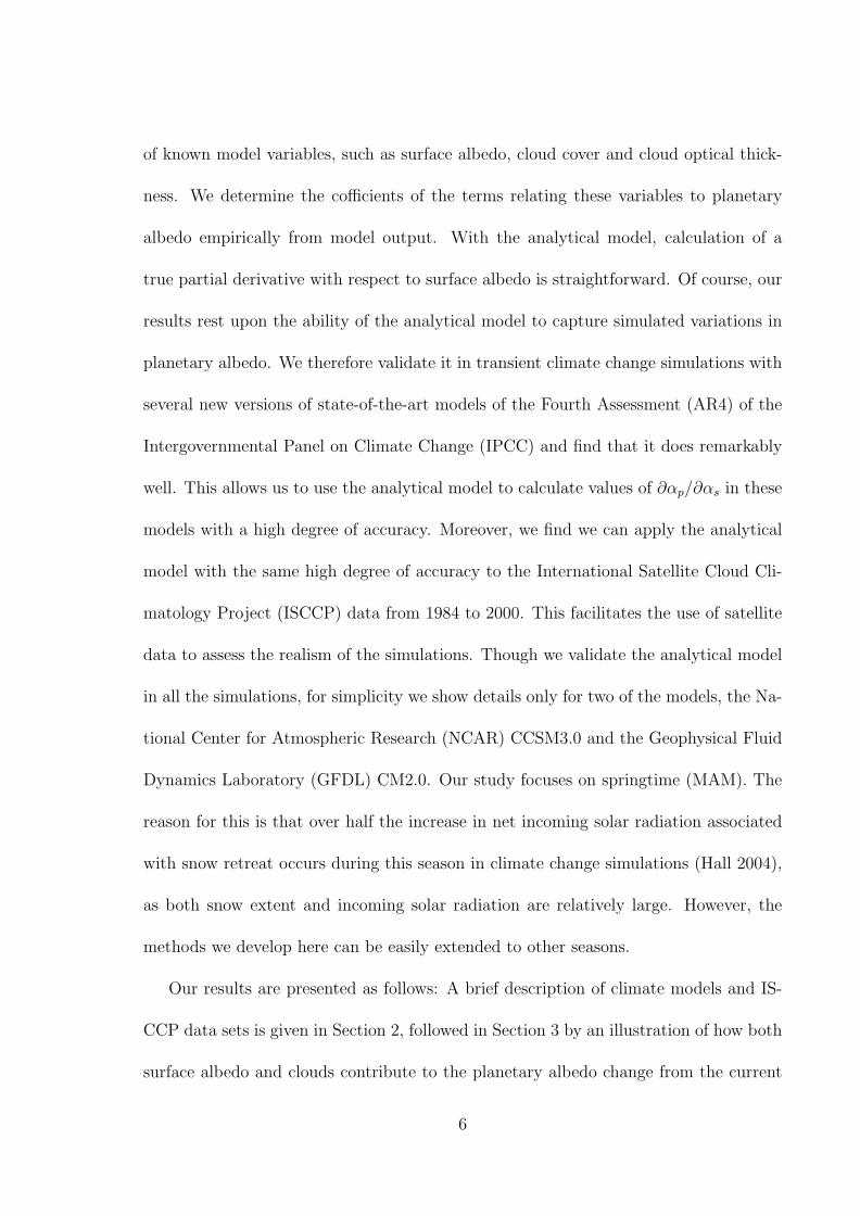
of known model variables, such as surface albedo, cloud cover and cloud optical thick-

ness. We determine the cofficients of the terms relating these variables to planetary

albedo empirically from model output. With the analytical model, calculation of a

true partial derivative with respect to surface albedo is straightforward. Of course, our

results rest upon the ability of the analytical model to capture simulated variations in

planetary albedo. We therefore validate it in transient climate change simulations with

several new versions of state-of-the-art models of the Fourth Assessment (AR4) of the

Intergovernmental Panel on Climate Change (IPCC) and find that it does remarkably

well. This allows us to use the analytical model to calculate values of ∂αp/∂αs in these

models with a high degree of accuracy. Moreover, we find we can apply the analytical

model with the same high degree of accuracy to the International Satellite Cloud Cli-

matology Project (ISCCP) data from 1984 to 2000. This facilitates the use of satellite

data to assess the realism of the simulations. Though we validate the analytical model

in all the simulations, for simplicity we show details only for two of the models, the Na-

tional Center for Atmospheric Research (NCAR) CCSM3.0 and the Geophysical Fluid

Dynamics Laboratory (GFDL) CM2.0. Our study focuses on springtime (MAM). The

reason for this is that over half the increase in net incoming solar radiation associated

with snow retreat occurs during this season in climate change simulations (Hall 2004),

as both snow extent and incoming solar radiation are relatively large. However, the

methods we develop here can be easily extended to other seasons.

Our results are presented as follows: A brief description of climate models and IS-

CCP data sets is given in Section 2, followed in Section 3 by an illustration of how both

surface albedo and clouds contribute to the planetary albedo change from the current

6

to the future climate in the NH extratropics using the CM2.0 and CCSM3.0 simula-

tions as examples. An analytical model for planetary albedo is developed and validated

against simulated and ISCCP data sets in Section 4. In Section 5, we use this model to

obtain an expression for ∂αp/∂αs and assess it in the current and future climate based

on simulated and ISCCP data sets. Summary and implications are found in Section 6,

where we also present calculations of the ∆αs/∆Ts term of eq. (1) for the AR4 models.

In this section we compare the intermodel divergence in this term to the divergence in

the ∂αp/∂αs term to see which accounts for the most overall intermodel divergence in

simulations of snow albedo feedback.

2. Models and observations

2.1 Models

We use output from the 20th and 22nd centuries of transient climate change ex-

periments with 17 AR4 models (see Table 1). The 20th century climate is simulated

in these models by imposing estimates of climate forcings from the period 1901-2000,

while the 22nd century is simulated by imposing the A1B emissions scenario (Prentice

et al. 2001).

Since the analytical model is validated in detail only for NCAR CCSM3.0 and GFDL

CM2.0 models, only these two models are briefly described here. NCAR CCSM3.0 (re-

ferred to hereafter as CCSM3.0) consists of general circulation models of the atmosphere

and ocean, a land surface model and a sea-ice model. The atmospheric component

(Collins et al. 2004) has horizontal resolution of approximately 1.40 latitude by 1.40

longitude and 26 vertical finite difference levels. The land surface component contains

7

a simplified treatment of surface processes responsible for land-atmosphere exchange of

heat, water and momentum (Oleson et al. 2004). A canopy radiative transfer scheme

is used to calculate surface albedo, accounting for the joint albedo effect of canopy

and ground. Ground albedo is a weighted combination of soil and snow albedos by

snow cover, which in turn is a function of snow depth. Snow albedo is parameter-

ized as a function of solar zenith angle and snow age. The oceanic component (Smith

and Gent 2004) has 320×384 points horizontally and 40 ocean levels vertically. The

sea-ice component includes a subgrid-scale ice thickness distribution, energy conserving

thermodynamics, and elastic-viscous-plastic dynamics (Briegleb et al. 2004).

Similar to CCSM3.0, the GFDL CM2.0 (referred to hereafter as CM2.0) consists of

general circulation models of the atmosphere and ocean, a land surface model and a sea

ice model. The atmosphere component uses a new grid point dynamical core, a prog-

nostic cloud scheme and a multi-species aerosol climatology (GAMDT 2005). It has

horizontal resolution of 2.50 longitude by 20 latitude and 24 vertical levels. The land

component is based on the Land Dynamics model described by Milly and Shmakin

(2002). Surface albedo over snow-covered regions is parameterized as an average of

snow-free surface albedo and snow albedo, which are weighted by snow cover. Snow

cover is in turn a function of snow depth. Snow albedo is parameterized as a function

of surface temperature. This scheme does not explicitly include canopy effects in its

calculation of surface albedo, as is the case with CCSM3.0. The model has a full 3-

dimensional dynamical ocean as well as a complex sea ice model; however, no official

documentation of the ocean and sea ice components of CM2.0 was available when this

article was composed.

8

2.2 ISCCP data sets

The ISCCP D-series cloud data sets used in this study are based on observations from

a suite of operational weather satellites measuring the temporal and spatial distribution

of visible (VIS wavelength ≈ 0.6 µm), near-infrared (NIR wavelength ≈ 3.7 µm) and

infrared (IR wavelength ≈ 11 µm) radiation. These measurements are then employed

to retrieve information about clouds, such as cloud cover, cloud optical thickness and

cloud top pressure (Rossow and Schiffer 1991; Rossow and Garder 1993a,b; Rossow

et al. 1993; Rossow and Schiffer 1999). Three changes have been made in the D-

series datasets to enhance the accuracy of cloud detection over snow- and ice-covered

surfaces (Rossow and Schiffer 1999):(1) most importantly, a new threshold test on 3.7

µm radiances was used, exploiting significantly greater contrast between cloudy and

clear scenes over snow- and ice-covered surfaces at this frequency than at 0.6 µm;

(2) at the high latitudes, the visible radiance threshold test was changed to a visible

reflectance threshold test; (3) over snow and ice in the polar regions, both the VIS and

IR thresholds were lowered. Together these improvements have been shown to increase

significantly low-level cloud detection sensitivity over snow and ice and reduce the biases

in cloud optical thickness of previous ISCCP C-series datasets in these regions.

Accompanying the ISCCP D-series cloud data sets are radiative flux data sets con-

taining solar and infrared radiative fluxes at the TOA and surface for both clear-sky

and full-sky situations. They are calculated by specifying the following information in

a radiative transfer model (Zhang et al. 2004): (1) atmospheric temperature and hu-

midity profiles; (2) vertical profiles of various atmospheric gases, such as CO2, O3, O2

9

and CH4; (3) vertical aerosol profiles for the troposphere and stratosphere; (4) ISCCP

D-series cloud datasets; (5) snow and ice cover data. All the data mentioned above are

time-varying so that observed variations in radiative properties of the atmosphere and

surface are reflected in the fluxes at the TOA and surface.

These data sets are provided on a global 2.50 × 2.50 grid and cover the period from

1984 to 2000.

3. Simulated reduction in planetary albedo over NH extratrop-

ical land areas

In this section, we demonstrate how both surface albedo and clouds contribute to

the planetary albedo change from the current to the future climate in NH extratropical

land areas using the CM2.0 and CCSM3.0 simulations as examples.

Fig 1 shows simulated changes in springtime surface albedo (αs), cloud cover (c),

logarithm of cloud optical thickness (ln(τ + 1)) and planetary albedo (αp) from the

20th to the 22nd century climate in the NH extratropics. We show the logarithm of

cloud optical thickness (τ) rather than τ itself to take account of the quasi-logarithmic

dependence of cloud albedo on τ (Rossow et al. 1996). Because cloud liquid water path

(clwp) and ice water path (ciwp) rather than τ are provided by the CM2.0 and CCSM3.0

data sets, a relation is used to convert clwp and ciwp into τ :

τ = κ1 · clwp + κ2 · ciwp (3)

where κ1 and κ2 are assumed to be 0.16 and 0.10, respectively, in accordance with

10

the values used by the ISCCP (Rossow et al. 1996). This facilitates the comparison

between ISCCP data sets and model data sets in the current climate in Sections 4 and

5.

As shown in Fig 1, surface albedo decreases in the warmer climate in both CM2.0

and CCSM3.0 throughout the NH extratropical land areas, especially northern Canada,

western Russia and Tibetan plateau. However, the decrease is much greater in CM2.0

than CCSM3.0. The surface albedo reductions averaged over extratropical North Amer-

ica and Eurasia in CM2.0 are about 5-8%, but are only about 3-4% in CCSM3.0 (see

Fig 2). The surface albedo reduction in CCSM3.0 is smaller because surface albedo

is less sensitive to the change in surface air temperature and also because the overall

warming is smaller in the model. As shown in Table 2, the ratio, ∆αs/∆Ts in CCSM3.0

is about 10% and 50% smaller than that of CM2.0 in extratropical Eurasia and North

America.

Changes in cloud cover and cloud optical thickness simulated in CM2.0 and

CCSM3.0 differ not only in amplitude, but also in sign. Cloud cover in CM2.0 decreases

in the warmer climate nearly everywhere in North America and Eurasia, especially in

the western United States and western Europe. This reduction averaged over extrat-

ropical North America and Eurasia is about 1% and 4% (see Fig 2). In contrast, cloud

cover simulated in CCSM3.0 increases in the high latitudes of Eurasia and nearly ev-

erywhere in North America, especially in northern Canada, and decreases only in the

middle latitudes of Eurasia. Cloud cover averaged over extratropical North America

increases 2%, but decreases 1% over extratropical Eurasia (see Fig 2). The logarithm

of cloud optical thickness in CM2.0 increases in the warmer climate nearly everywhere

11

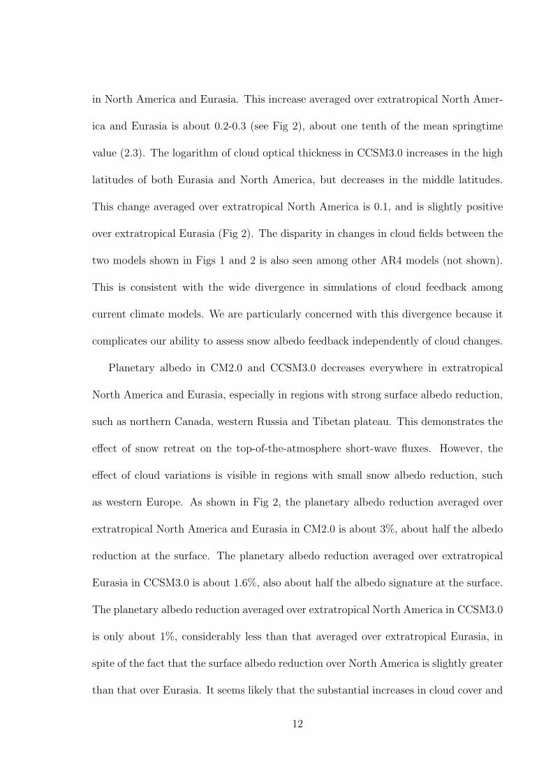
in North America and Eurasia. This increase averaged over extratropical North Amer-

ica and Eurasia is about 0.2-0.3 (see Fig 2), about one tenth of the mean springtime

value (2.3). The logarithm of cloud optical thickness in CCSM3.0 increases in the high

latitudes of both Eurasia and North America, but decreases in the middle latitudes.

This change averaged over extratropical North America is 0.1, and is slightly positive

over extratropical Eurasia (Fig 2). The disparity in changes in cloud fields between the

two models shown in Figs 1 and 2 is also seen among other AR4 models (not shown).

This is consistent with the wide divergence in simulations of cloud feedback among

current climate models. We are particularly concerned with this divergence because it

complicates our ability to assess snow albedo feedback independently of cloud changes.

Planetary albedo in CM2.0 and CCSM3.0 decreases everywhere in extratropical

North America and Eurasia, especially in regions with strong surface albedo reduction,

such as northern Canada, western Russia and Tibetan plateau. This demonstrates the

effect of snow retreat on the top-of-the-atmosphere short-wave fluxes. However, the

effect of cloud variations is visible in regions with small snow albedo reduction, such

as western Europe. As shown in Fig 2, the planetary albedo reduction averaged over

extratropical North America and Eurasia in CM2.0 is about 3%, about half the albedo

reduction at the surface. The planetary albedo reduction averaged over extratropical

Eurasia in CCSM3.0 is about 1.6%, also about half the albedo signature at the surface.

The planetary albedo reduction averaged over extratropical North America in CCSM3.0

is only about 1%, considerably less than that averaged over extratropical Eurasia, in

spite of the fact that the surface albedo reduction over North America is slightly greater

than that over Eurasia. It seems likely that the substantial increases in cloud cover and

12

cloud optical thickness over North America are responsible for this disproportionately

small reduction in planetary albedo, highlighting the need for a method to quantify the

dependence of planetary albedo on surface albedo independently of cloud variations.

4. An analytical model to understand planetary albedo

In the previous section, we showed that surface albedo, cloud cover and cloud op-

tical thickness probably all contribute to the simulated planetary albedo change in the

warmer climate in two AR4 transient climate change simulations. To isolate the surface

contribution, we develop an analytical model governing planetary albedo, and validate

it against simulated and satellite-based data sets. This model relates full-sky planetary

albedo to known quantities, including clear-sky planetary albedo, cloud cover, cloud

optical thickness and surface albedo. This allows us to generate an analytical expres-

sion for ∂αp/∂αs. We can then compare this quantity among models and satellite-based

data sets.

This model is derived as follows: Full-sky planetary albedo can be written as the

weighted mean of clear-sky planetary albedo (αcrp ) and cloudy-sky planetary albedo

(αcdp ):

αp = (1− c) · αcrp + c · αcd

p (4)

In eq. (4), αcrp is given as follows:

αcrp = αcr

a + T cra · αs (5)

which is the sum of clear-sky atmospheric albedo to incoming solar radiation (αcra ),

13

and a surface albedo component, which is the product of αs and an effective clear-sky

atmospheric transmissivity, T cra . In eq. (4), αcd

p is given as follows:

αcdp = αcd

a + T cda · αs (6)

which is the sum of cloudy sky atmospheric albedo to incoming solar radiation (αcda ),

and a surface albedo component, which is the product of αs and an effective cloudy sky

atmospheric transmissivity, T cda . We model the difference between clear and cloudy sky

atmospheric albedo as proportional to the logarithm of cloud optical thickness, thereby

linking αcra in eq. (5) and αcd

a in eq. (6):

αcda = αcr

a + ε1 · ln(τ + 1) (7)

In eq. (7), ε1 is the linear coefficient relating the logarithm of cloud optical thickness

to the cloudy-sky atmospheric albedo. Similarly, we model the difference between clear

and cloudy sky effective transmissivity as proportional to the logarithm of cloud optical

thickness, thereby linking T cra in eq. (5) and T cd

a in eq. (6):

T cda = T cr

a − ε2 · ln(τ + 1) (8)

where ε2 is the linear coefficient relating the logarithm of cloud optical thickness to the

effective cloudy-sky atmospheric transmissivity.

14

We plug eqs. (5)-(8) into (4), and rearrange it into

αp = αcrp + c · ln(τ + 1) · (ε1 − ε2 · αs) (9)

We can rewrite eq. (9) as follows:

αp − αcrp = ε1 · c · ln(τ + 1)− ε2 · c · ln(τ + 1) · αs (10)

Because αp, αcrp , c, ln(τ + 1) and αs are given in models and observations, values of the

two linear coefficients, ε1 and ε1, can be readily obtained by regressing (αp − αcrp ) onto

c · ln(τ + 1) and c · ln(τ + 1) · αs.

Eq. (9) is our analytical model for planetary albedo. To test how well it captures

planetary albedo and its temporal and spatial variability, we apply it to ISCCP and the

AR4 simulations of the current climate. First, αp, αcrp , c, ln(τ + 1) and αs in March,

April and May were averaged to get a yearly time-series of springtime-mean values at

each location within extratropical North America and Eurasia. The time period used

was the 20th century in the case of the AR4 simulations and the years 1984-2000 for the

ISCCP data set. Then, the difference between full-sky and clear-sky planetary albedo,

(αp − αcrp ) was regressed onto c · ln(τ + 1) and c · ln(τ + 1) · αs to obtain values of ε1

and ε2. We perform the regression calculation based on concantenated time series of all

locations within extratropical North America and Eurasia, so that we are attempting

to capture both interannual and geographical variability in planetary albedo. This

provides samples large enough to achieve stable statistics in both satellite data sets and

15

simulations, the size of samples being larger than 8000. We can then model interannual

and geographical variations in planetary albedo by plugging in these values of ε1 and

ε2, as well as values of c, τ , αcrp and αs into eq. (9). As a example, Fig 3 shows the

scatterplot of modeled planetary albedo against actual planetary albedo in ISCCP data

sets and two simulations: CM2.0 and CCSM3.0. They almost exactly follow a diagonal

line, and the correlation coefficient shown in the right-bottom corner of each panel is

very close to unity, implying nearly perfect agreement. Eq. (9) is also used to model

planetary albedo in the climate of the 22nd century in CM2.0 and CCSM3.0 by plugging

in the values of ε1 and ε2 obtained from the current climate, as well as values of c, τ , αcrp

and αs in the future climate. Similarly, modeled and simulated planetary albedo in the

two models are nearly perfectly correlated (not shown). Eq. (9) captures the physical

relationship seen in the models and ISCCP data set among planetary albedo, surface

albedo and clouds extremely well not only in the CCSM3.0 and CM2.0 simulations,

but also the other AR4 models. Plots for the other AR4 models similar to Fig. 3 (not

shown) are almost identical, with a nearly one-to-one correspondence between modeled

and simulated planetary albedo.

To reveal physical insights behind eq. (9), we rearrange it:

αp = (αcra + ε1 · c · ln(τ + 1)) + (T cr

a − ε2 · c · ln(τ + 1)) · αs (11)

The first term, (αcra + ε1 · c · ln(τ + 1)) in eq. (11) can be viewed as an effective full-sky

atmospheric albedo. It is attributed partly to the clear-sky atmosphere (αcra ) and partly

to clouds (ε1 ·c · ln(τ +1)). The second term, (T cra −ε2 ·c · ln(τ +1)) ·αs can be viewed as

16

a surface albedo component of full-sky planetary albedo, which is the product of αs and

an effective full-sky atmospheric transmissivity (T cra − ε2 · c · ln(τ +1)). The latter is at-

tributed partly to the clear-sky atmosphere (T cra ) and partly to clouds (−ε2 ·c·ln(τ +1)).

The two terms involving clouds in eq. (11), (ε1 · c · ln(τ +1)) and (−ε2 · c · ln(τ +1) ·αs)

represent two effects on planetary albedo: (1) clouds increase planetary albedo through

their own reflectivity; (2) clouds decrease the surface contribution to planetary albedo

by reducing the effective full-sky atmospheric transmissivity. In both cases, the effect is

proportional to the product of cloud cover and the logarithm of cloud optical thickness.

5. Dependence of planetary albedo on surface albedo (∂αp/∂αs)

Eq. (11) is such a successful model for planetary albedo that we can use it to derive

an accurate expression for the first term of eq. (1), the partial derivative, ∂αp/∂αs:

∂αp/∂αs = T cra − ε2 · c · ln(τ + 1) (12)

The right-hand side of eq. (12) represents the total attenuation effect of the atmosphere

on the surface’s contribution to planetary albedo fluctuation. This includes a contri-

bution from the cloudless atmosphere, represented by T cra , as well as a contribution

from cloud, being proportional to the product of cloud cover and the logarithm of cloud

optical thickness. The direct effects of the changes in cloudiness on planetary albedo

are not included in eq. (12), and so are not conflated with the effects of changes in

surface albedo, as is the case if the dependence of planetary albedo on surface albedo is

measured by simply regressing planetary albedo variations onto their counterparts at

17

the surface. This points to the relevance of our analytical model in unraveling surface

and cloud’s contributions to planetary albedo variations in cryosphere regions. We will

use eq. (12) to assess the values of ∂αp/∂αs in the current climate and future climate.

The quantities c and τ are given by the ISCCP and model data sets, while ε2 is

known from regression analysis relying on eq. (10). The unknown quantity on the right-

hand side of eq. (12) is therefore the clear-sky effective atmospheric transmissivity, T cra .

Relying on eq. (5), we can obtain it by regressing clear-sky planetary albedo, αcrp onto

surface albedo, αs. In analogy with Fig 3, we show a scatterplot of modeled clear-sky

planetary albedo against the actual clear-sky planetary albedo in ISCCP, CM2.0 and

CCSM3.0 data sets in Fig 4 as a validation of this regression model. They follow a

diagonal line almost exactly and the correlation coefficient, shown in the right-bottom

corner of each scatterplot, is very close to unity, implying nearly perfect agreement.

Fig 5 shows values of T cra seen in ISCCP, CM2.0 and CCSM3.0 in North America and

Eurasia. Values of T cra in the current climate are comparable among ISCCP, CM2.0 and

CCSM3.0, and in the future climate between CM2.0 and CCSM3.0 in both continents,

being about 0.7. This is also true for other simulations (not shown). The clear-sky

atmosphere attenuates surface albedo fluctuations so that their magnitudes are consis-

tently reduced by about 30% as they are mirrored in planetary albedo variations.

According to Fig 5, there is also a reasonable agreement in values of ε2 ·c·ln(τ +1) in

the current and future climate in both continents, all being about 1/3 as large as values

of T cra . Values of ε2 ·c · ln(τ +1) are relatively small because clouds over the extratropics

are generally not very thick (mean values of ln(τ +1) is about 2.3) compared to deeper

clouds in the tropics (mean values of ln(τ +1) is about 4) and also because a substantial

18

fraction of the sky is clear in NH snow-covered regions (mean cloud cover is about 60-

70%). Because values of ε2, the regression coefficient relating cloud optical thickness to

cloudy sky transmissivity are generally smaller than 0.16 (see Table 3), differences in

values of ε2 · c · ln(τ + 1) in the current and future climate among the three data sets

are generally smaller than 0.1(see Table 3), in spite of the fact that cloud fields differ

somehow in the current and future climate among the three data sets (Table 3).

The mean values of ∂αp/∂αs seen in ISCCP, CM2.0 and CCSM3.0 in the current

and future climate have general agreement, all being about 0.5 (Fig 5), implying the

size of surface-induced planetary albedo fluctuations in the NH extratropics is about

half the albedo signature at the surface. This is the case in spite of the disparities in

cloud fields among ISCCP, CM2.0 and CCSM3, between North America and Eurasia

within individual data sets, and within regions going from the present-day to future

simulated climates. This demonstrates that disparities in the cloud fields seen in the

ISCCP, CM2.0 and CCSM3.0 are not large enough to generate appreciable divergence

in values of ∂αp/∂αs in the NH extratropics.

Based on eq. (12), values of ∂αp/∂αs in the other AR4 simulations are calcu-

lated and shown in Fig 6. The corresponding values in CM2.0 and CCSM3.0 are also

shown in this figure for comparison. Consistent with the agreement between CM2.0

and CCSM3.0, values of ∂αp/∂αs are comparable among all the simulations. The stan-

dard deviation of this quantity among all the simulations is 0.04, only about 8% of

the mean value (0.52) in both North America and Eurasia. Moreover, in the majority

of the simulations, values of ∂αp/∂αs agree with the ISCCP values (represented by

the solid lines in Fig 6) to within 10%. This indicates that the ∂αp/∂αs component

19

of snow albedo feedback simulated in climate models agrees quite well with observations.

6. Summary and Implications

The strength of snow albedo feedback can be quantified as the product of two terms,

one representing the dependence of planetary albedo on surface albedo (∂αp/∂αs), and

another representing the change in surface albedo induced by a unit temperature change

(∆αs/∆Ts). The ∂αp/∂αs term is the variation in planetary albedo with surface albedo

in NH extratropical land areas, with other factors such as water vapor concentration

and cloud fixed. However, cloud properties can change substantially over the course

of transient climate change experiments, and these can in turn have a large effect on

incoming solar radiation. This makes it particularly difficult to quantify the strength

of this aspect of snow albedo feedback.

To isolate the surface contribution from that of cloud, we develop an analytical model

governing planetary albedo. This model relates full-sky planetary albedo to known

quantities, including clear-sky planetary albedo, cloud cover, cloud optical thickness and

surface albedo. It captures both interannual and geographical variability in planetary

albedo in simulated and satellite-based data sets extremely well. The advantage of

this model is that we can use it to derive an expression for a true partial derivative of

planetary albedo with respect to surface albedo. It includes a contribution from the

cloudless atmosphere, represented by an effective clear-sky atmospheric transmissivity

as well as a contribution from cloud, being proportional to the product of cloud cover

and logarithm of cloud optical thickness.

There is good agreement in values of the clear-sky component of the atmosphere’s

20

attenuation of surface albedo anomalies, both in the current climate and in the future

climate in both North America and Eurasia, all being about 0.7. Values of the cloud

contribution to the variation in planetary albedo with surface albedo are about 1/3

the size of clear sky component. Cloud is not the most significant factor controlling

the variation in planetary albedo with surface albedo both because clouds over the

extratropics is generally not very thick, and because a substantial fraction of the sky is

clear in NH snow-covered regions. Therefore differences or errors in mean cloud fields

of the magnitude seen in the current generation of climate models are not large enough

to cause appreciable divergence or errors in estimates of the variation of planetary

albedo with surface albedo in the current climate. For example, differences in values

of the cloud contribution to the atmospheric attenuation effect among the three data

sets in the current climate are generally only about 10% of the total attenuation effect.

Nor are changes in mean cloud fields as a result of climate change large enough to

cause the variation of planetary albedo with surface albedo to exhibit significant time

dependence. Because of this relative insensitivity to variations in mean cloud fields,

the mean values of the variation of planetary albedo with surface albedo seen in the

simulated current and future climate are in general agreement, all being about 0.5. This

value is also in agreement with the satellite-based ISCCP data set. Therefore we can

say with a high degree of confidence that both in simulations and satellite-based data

sets, snow-induced planetary albedo anomalies are about half the albedo signature at

the surface.

Finally, armed with these conclusions about the ∂αp/∂αs term in eq. (1), we focus

on the second term in this equation: ∆αs/∆Ts. This term is related to surface processes

21

and represents the sensitivity of surface albedo to surface air temperature in the NH

extratropics. It is easily quantified in AR4 climate simulations, and we show the results

in Fig 7. This quantity varies a great deal from model to model. The standard deviation

of this quantity among all the simulations is about 1/3 of the mean value in both North

America and Eurasia, much greater than the relative variation in ∂αp/∂αs shown in Fig.

6. And over both North American and Eurasia, the largest value is approximately three

times as large as the smallest. Therefore we determine that this term is unquestionably

the main source of the large divergence in simulations of snow albedo feedback. To

reduce this divergence, attention should be focused on differing parameterizations of

surface processes rather than intermodel variations in the attenuation effect of the

atmosphere on surface albedo anomalies.

Acknowledgments. This study is based on model integrations performed by NCAR

and CRIEPI with support and facilities provided by NSF, DOE, ESC/JAMSTEC

and MEXT. The authors acknowledge the international modeling groups for providing

their data for analysis, the Program for Climate Model Diagnosis and Intercompari-

son (PCMDI) for collecting and archiving the model data, the JSC/CLIVAR Work-

ing Group on Coupled Modelling (WGCM) and their Coupled Model Intercomparison

Project (CMIP) and Climate Simulation Panel for organizing the model data analysis

activity, and the IPCC WG1 TSU for technical support. The IPCC Data Archive at

Lawrence Livermore National Laboratory is supported by the Office of Science, U.S.

Department of Energy. This study was supported by NSF Grant ATM-0135136. But,

any opinions, findings, and conclusions or recommendations expressed in this material

22

are those of the authors and do not necessarily reflect the views of the National Science

Foundation. The authors wish to thank Y.-C. Zhang for his help with the ISCCP cloud

and flux datasets and two anonymous reviewers for their constructive criticism of this

manuscript.

23

References

Briegleb, B. P. and coauthors, 2004: Scientific Description of the Sea Ice Component

in the Community Climate System Model, Version Three. NCAR/TN-463+STR,

NCAR TECHNICAL NOTE.

Cess, R. D. and coauthors, 1991: Interpretation of snow-climate feedback as produced

by 17 general circulation models. Science, 253, 888–892.

Cess, R. D. and G. L. Potter, 1988: A methodology for understanding and intercompar-

ing atmospheric climate feedback processes in general circulation models. J. Geophys.

Res., 93(D7), 8305–8314.

Collins, W. D. and coauthors, 2004: Description of the NCAR Community Atmosphere

Model (CAM3.0). NCAR/TN-464+STR, NCAR TECHNOCAL NOTE.

Cubasch, U. and coauthors, 2001: Projections of future climate change. Climate Change

2001:The Scientific Basis. J. W. Kim and J. Stone, Eds., Cambridge University Press,

525-582.

GAMDT, 2005: The new GFDL global atmosphere and land model AM2/CM2.0: Eval-

uation with prescribed SST simulations. Submitted to J. Climate.

Groisman, P. Y., T. R. Karl and R. W. Knight, 1994a: Observed impact of snow cover

on the heat balance and the rise of continental spring temperatures. Science, 263,

198–200.

Groisman, P. Y., T. R. Karl and R. W. Knight, 1994b: Changes of snow cover, tem-

24

peratures, and radiative heat balance over the northern hemisphere. J. Climate, 7,

1633–1656.

Hall, A., 2004: The role of surface albedo feedback in climate. J. Climate, 17, 1550–

1568.

Holland, M. M. and C. M. Bitz, 2003: Polar amplification of climate change in coupled

models. Climate Dyn., 21, 221–232.

Milly, P. C. D. and A. B. Shmakin, 2002: Global modeling of land water and energy

balances. Part I: The land dynamics (LaD) model. J. Hydrometeorology, 3(3), 283–

299.

Oleson, K. W. and coauthors, 2004: Techical Description of the Community Land

Model (CLM). NCAR/TN-464+STR, NCAR TECHNOCAL NOTE.

Prentice, I. C. and coauthors, 2001: The carbon cycle and atmospheric carbon dioxide.

Climate Change 2001:The Scientific Basis. L. Pitelka and A. Ramirez Rojas, Eds.,

Cambridge University Press, 183-237.

Randall, D. A. and coauthors, 1994: Analysis of snow feedbacks in 14 general circulation

models. J. Geophys. Res., 99(D10), 20757–20772.

Rossow, W. B. and L. C. Garder, 1993a: Cloud detction using satellite measurements

of infrared and visible radiances for ISCCP. J. Climate, 6, 2341–2369.

Rossow, W. B. and L. C. Garder, 1993b: Validation of ISCCP cloud detections. J.

Climate, 6, 2370–2393.

25

Rossow, W. B. and R. A. Schiffer, 1991: ISCCP cloud data products. Bull. Amer.

Meteor. Soc., 72(1), 2–20.

Rossow, W. B. and R. A. Schiffer, 1999: Advances in understanding clouds from ISCCP.

Bull. Amer. Meteor. Soc., 80(11), 2261–2287.

Rossow, W. B., A. W. Walker, D. Beuschel and M. Roiter, 1996: International Satillite

Cloud Climatological Project (ISCCP) description of new cloud datasets. WMO/TD

737, World Climate Research Programme (ICSU AND WMO).

Rossow, W. B., A. W. Walker and L. C. Garder, 1993: Comparison of ISCCP and other

cloud amounts. J. Climate, 6, 2394–2418.

Smith, R. and P. Gent, 2004: Reference Manual for the Parallel Ocean Program POP:

Ocean System Model CCSM2.0 AND 3.0. LAUR-02-2484.

Zhang, Y.-C., W. B. Rossow, A. A. Lacis, V. Oinas and M. M. Mishchenko, 2004:

Calculation of radiative fluxes from the surface to top of atmosphere based on ISCCP

and other global datasets: Refinements of the radiative transfer model and the input

data. J. Geophys. Res., 109(D19105), 1–27.

26

Figure captions:

Figure 1: The geographical distribution of changes in climatological springtime-mean

surface albedo (αs), cloud cover (c), logarithm of cloud optical thickness (ln(τ + 1))

and planetary albedo (αp) from the climate of the 20th century (1901-2000) to the

climate of the 22nd century (2100-2199) in CM2.0 and CCSM3.0 scenario runs. Here,

the changes in surface albedo, cloud cover and planetary albedo are all evaluated by

percentage points, rather than a fractional change. Surface albedo, cloud cover and

planetary albedo are in the units of %, while logarithm of cloud optical thickness is in

units of tenths. The same units for each variable are also used in Fig 2.

Figure 2: Changes in climatological springtime-mean surface albedo (αs), cloud cover

(c), logarithm of cloud optical thickness (ln(τ +1)) and planetary albedo (αp) averaged

over extratropical North America and Eurasia from the climate of the 20th century

(1901-2000) to the climate of the 22nd century (2100-2199) in CM2.0 and CCSM3.0. In

the calculations, changes in the climatological springtime-mean values of c, ln(τ+1) and

αp, as shown in Fig 1, were weighted by climatological incoming solar radiation at the

top of atmosphere in the climate of the 20th century, while changes in the climatological

springtime-mean values of αs were weighted by climatological incoming solar radiation

at the surface in the climate of the 20th century. These techniques were used in all

calculations involving spatial averages of c, ln(τ + 1), αp and αs in this article. Note

that extratropical North America encompasses land area northward of 300N, including

Greenland, and extratropical Eurasia is the Eurasian land area northward of 300N.

Figure 3: Scatter plots of modeled interannual and geographical variations in springtime-

mean planetary albedo based on eq. (10) and interannual and geographical variations

27

in springtime-mean planetary albedo seen in ISCCP, CM2.0 and CCSM3.0 in extrat-

ropical North America and Eurasia for the current climate. The current climate refers

to the climate of the 1984-2000 period for ISCCP, and the climate of the 20th century

for CM2.0 and CCSM3.0. (These same definitions apply to whole paper.) Here, for

clarity, we only show 10% of ISCCP data sets and 1% of the two model data sets on

this figure. All sub-samples are randomly chosen. This same plotting method is also

used in Fig 4.

Figure 4: Scatter plots of modeled interannual and geographical variations in springtime-

mean clear-sky planetary albedo and interannual and geographical variations in springtime-

mean clear-sky planetary albedo seen in ISCCP, CM2.0 and CCSM3.0 in extratropical

North America and Eurasia for the current climate.

Figure 5: The climatological springtime-mean values of T cra , ε2·c·ln(τ+1) and ∂αp/∂αs

seen in ISCCP, CM2.0 and CCSM3.0 in extratropical North America and Eurasia in

the current climate and the future climate (2100-2199). First, regression calculations

are performed to obtain values of T cra , ε1 and ε2 based on eqs. (5) and (10) (see Sections

4 and 5). Then, climatological springtime-mean values of ε2 · c · ln(τ +1) are calculated

at all locations within extratropical North America and Eurasia. Finally, these values

are averaged over extratropical North America and Eurasia, respectively. Note that

∂αp/∂αs = T cra − ε2 · c · ln(τ + 1).

Figure 6: Values of ∂αp/∂αs in extratropical North America and Eurasia in climate

simulations. Procedures similar to those demonstrated in the caption of Fig 5 are

performed to get these values. See Table 1 for the names of the models. Values of

∂αp/∂αs are available only for 14 of the 17 models because other 4 models do not

28

provide all variables required by our analytical model. The solid lines in the figure

represent the ISCCP values of ∂αp/∂αs.

Figure 7: Values of ∆αs/∆Ts in extratropical North America and Eurasia in climate

simulations. Procedures similar to those demonstrated in the caption of Table 2 are

performed to get these values. The units are %/◦C.

29

Table captions:

Table 1: A list of 17 models used in this study and the numbers they correspond to

in Figs 6 and 7.

Table 2: First row: The changes in climatological springtime-mean surface albedo

(the first column), surface air temperature (the second column) averaged over North

America from the climate of the 20th century, 1901-2000 to the climate of the 22nd

century, 2100-2199 and the ratio of the former to the latter (the third column) in

CM2.0. Second row: As in the first row, except for Eurasia. Third row: As in the

first row, except for CCSM3.0 data sets. Fourth row: As in the second row, except for

CCSM3.0 data sets. Surface albedo is in units of % and surface air temperature is in

units of ◦C.

Table 3: First row: The climatological springtime-mean values of ε2 (the first column),

c · ln(τ +1) (the second column) in the climate of the 20th century and c · ln(τ +1) (the

third column) in the climate of the 22nd century in CM2.0 over extratropical North

America. Second row: As in the first row, except for extratropical Eurasia. Third row:

As in the first row, except for CCSM3.0 data sets. Fourth row: As in the second row,

except for CCSM3.0 data sets. Fifth row: The climatological springtime-mean values of

ε2 (the first column), c · ln(τ +1) (the second column) over extratropical North America

seen in ISCCP in the current climate, 1984-2000. Sixth row: As in the fifth row, except

for extratropical Eurasia.

CM2.0 CCSM3.0

∆ αs

−48

−36

−24

−12

0

∆ c−12

−8

−4

0

4

∆ln(τ+1)−4

−2

0

2

4

∆ αp

−8

−4

0

4

Figure 1: The geographical distribution of changes in climatological springtime-meansurface albedo (αs), cloud cover (c), logarithm of cloud optical thickness (ln(τ + 1))and planetary albedo (αp) from the climate of the 20th century (1901-2000) to theclimate of the 22nd century (2100-2199) in CM2.0 and CCSM3.0 scenario runs. Here,the changes in surface albedo, cloud cover and planetary albedo are all evaluated bypercentage points, rather than a fractional change. Surface albedo, cloud cover andplanetary albedo are in the units of %, while logarithm of cloud optical thickness is inunits of tenths. The same units for each variable are also used in Fig 2.

−8

−4

0

4CM2.0

∆ αs ∆ c ∆ ln (τ+1) ∆ α

p

−8

−4

0

4CCSM3.0

∆ αs ∆ c ∆ ln (τ+1) ∆ α

p

NAEU

Figure 2: Changes in climatological springtime-mean surface albedo (αs), cloud cover(c), logarithm of cloud optical thickness (ln(τ +1)) and planetary albedo (αp) averagedover extratropical North America and Eurasia from the climate of the 20th century(1901-2000) to the climate of the 22nd century (2100-2199) in CM2.0 and CCSM3.0. Inthe calculations, changes in the climatological springtime-mean values of c, ln(τ+1) andαp, as shown in Fig 1, were weighted by climatological incoming solar radiation at thetop of atmosphere in the climate of the 20th century, while changes in the climatologicalspringtime-mean values of αs were weighted by climatological incoming solar radiationat the surface in the climate of the 20th century. These techniques were used in allcalculations involving spatial averages of c, ln(τ + 1), αp and αs in this article. Notethat extratropical North America encompasses land area northward of 300N, includingGreenland, and extratropical Eurasia is the Eurasian land area northward of 300N.

15

30

45

60

75North America

ISCCP

0.99

Eurasia

ISCCP

0.99

15

30

45

60

75CM2.0

mo

del

ed p

lan

etar

y al

bed

o (

%)

0.99

CM2.0

0.99

15 30 45 60 7515

30

45

60

75CCSM3.0

0.99

15 30 45 60 75

CCSM3.0

0.99

planetary albedo (%)

Figure 3: Scatter plots of modeled interannual and geographical variations inspringtime-mean planetary albedo based on eq. (10) and interannual and geographicalvariations in springtime-mean planetary albedo seen in ISCCP, CM2.0 and CCSM3.0 inextratropical North America and Eurasia for the current climate. The current climaterefers to the climate of the 1984-2000 period for ISCCP, and the climate of the 20thcentury for CM2.0 and CCSM3.0. (These same definitions apply to whole paper.) Here,for clarity, we only show 10% of ISCCP data sets and 1% of the two model data sets onthis figure. All sub-samples are randomly chosen. This same plotting method is alsoused in Fig 4.

5

19

33

47

61

75North America

ISCCP

0.99

Eurasia

ISCCP

0.99

5

19

33

47

61

75CM2.0

mo

del

ed c

lear−s

ky p

lan

etar

y al

bed

o (

%)

0.99

CM2.0

0.99

5 19 33 47 61 75 5

19

33

47

61

75CCSM3.0

0.99

5 19 33 47 61 75

CCSM3.0

0.99

clear−sky planetary albedo (%)

Figure 4: Scatter plots of modeled interannual and geographical variations inspringtime-mean clear-sky planetary albedo and interannual and geographical variationsin springtime-mean clear-sky planetary albedo seen in ISCCP, CM2.0 and CCSM3.0 inextratropical North America and Eurasia for the current climate.

0

0.5

1 contribution of atmosphere

1984−2000

ISCCP

1901−2000 2100−2199

CM2.0

1901−2000 2100−2199

CCSM3.0

0

0.5

1 contribution of clouds

1984−2000

ISCCP

1901−2000 2100−2199

CM2.0

1901−2000 2100−2199

CCSM3.0

0

0.5

1 total

1984−2000

ISCCP

1901−2000 2100−2199

CM2.0

1901−2000 2100−2199

CCSM3.0

NA EU

Figure 5: The climatological springtime-mean values of T cra , ε2 ·c·ln(τ +1) and ∂αp/∂αs

seen in ISCCP, CM2.0 and CCSM3.0 in extratropical North America and Eurasia inthe current climate and the future climate (2100-2199). First, regression calculationsare performed to obtain values of T cr

a , ε1 and ε2 based on eqs. (5) and (10) (see Sections4 and 5). Then, climatological springtime-mean values of ε2 · c · ln(τ +1) are calculatedat all locations within extratropical North America and Eurasia. Finally, these valuesare averaged over extratropical North America and Eurasia, respectively. Note that∂αp/∂αs = T cr

a − ε2 · c · ln(τ + 1).

1 2 3 4 5 6 7 8 9 10 11 12 13 14 15 16 17 0

0.5

1North America

mean: 0.52std: 0.04

no

t av

aila

ble

no

t av

aila

ble

no

t av

aila

ble

no

t av

aila

ble

∂ α

p/ ∂

αs

CC

SM

3.0

CM

2.0

1 2 3 4 5 6 7 8 9 10 11 12 13 14 15 16 17 0

0.5

1Eurasia

mean: 0.51std: 0.04

no

t av

aila

ble

no

t av

aila

ble

no

t av

aila

ble

no

t av

aila

ble

∂ α

p/ ∂

αs

CC

SM

3.0

CM

2.0

Figure 6: Values of ∂αp/∂αs in extratropical North America and Eurasia in climatesimulations. Procedures similar to those demonstrated in the caption of Fig 5 areperformed to get these values. See Table 1 for the names of the models. Values of∂αp/∂αs are available only for 14 of the 17 models because other 4 models do notprovide all variables required by our analytical model. The solid lines in the figurerepresent the ISCCP values of ∂αp/∂αs.

1 2 3 4 5 6 7 8 9 10 11 12 13 14 15 16 17 0

−1

−2North America

mean: 0.84std: 0.31

∆ α

s/ ∆ T

s

CC

SM

3.0

CM

2.0

1 2 3 4 5 6 7 8 9 10 11 12 13 14 15 16 17 0

−1

−2Eurasia

mean: 0.75std: 0.25

∆ α

s/ ∆ T

s

CC

SM

3.0

CM

2.0

Figure 7: Values of ∆αs/∆Ts in extratropical North America and Eurasia in climatesimulations. Procedures similar to those demonstrated in the caption of Table 2 areperformed to get these values. The units are %/◦C.

Number Model

1 cnrm cm3

2 mri cgcm2 3 2a

3 giss model e r

4 csiro mk3 0

5 ncar pcm1

6 ukmo hadcm3

7 cccma cgcm3 1

8 iap fgoals1 0 g

9 mpi echam5

10 ukmo hadgem1

11 miub echo g

12 ipsl cm4

13 ncar ccsm3.0

14 miroc3 2 medres

15 inmcm3.0

16 gfdl cm2 0

17 gfdl cm2 1

Table 1: A list of 17 models used in this study and the numbers they correspond to in

Figs 6 and 7.

Regions ∆αs ∆Ts ∆αs/∆Ts

CM2.0 N. A. -8.17 5.58 -1.46

Eurasia -5.24 5.26 -1.00

CCSM3.0 N. A. -4.44 4.40 -1.01

Eurasia -3.59 3.97 -0.90

Table 2: First row: The changes in climatological springtime-mean surface albedo (the

first column), surface air temperature (the second column) averaged over North America

from the climate of the 20th century, 1901-2000 to the climate of the 22nd century, 2100-

2199 and the ratio of the former to the latter (the third column) in CM2.0. Second

row: As in the first row, except for Eurasia. Third row: As in the first row, except for

CCSM3.0 data sets. Fourth row: As in the second row, except for CCSM3.0 data sets.

Surface albedo is in units of % and surface air temperature is in units of ◦C.

Regions ε2 c · ln(τ + 1) (1901-2000) c · ln(τ + 1) (2100-2199)

CM2.0 N. A. 0.10 1.95 2.16

Eurasia 0.10 1.77 1.84

CCSM3.0 N. A. 0.16 1.65 1.77

Eurasia 0.16 1.40 1.54

ISCCP N. A. 0.14 1.51 —

Eurasia 0.14 1.35 —

Table 3: First row: The climatological springtime-mean values of ε2 (the first column),

c · ln(τ +1) (the second column) in the climate of the 20th century and c · ln(τ +1) (the

third column) in the climate of the 22nd century in CM2.0 over extratropical North

America. Second row: As in the first row, except for extratropical Eurasia. Third row:

As in the first row, except for CCSM3.0 data sets. Fourth row: As in the second row,

except for CCSM3.0 data sets. Fifth row: The climatological springtime-mean values of

ε2 (the first column), c · ln(τ +1) (the second column) over extratropical North America

seen in ISCCP in the current climate, 1984-2000. Sixth row: As in the fifth row, except

for extratropical Eurasia.