assessing ex-ante poverty &...
TRANSCRIPT

ASSESSING EX-ANTE POVERTY & DISTRIBUTIONAL
IMPACT OF MACROECONOMIC SHOCKS:
A MICRO- SIMULATION APPROACH
Module 2: Welfare Impact of Macroeconomic Shocks: Overview of Selected Tools

Outline
1. Motivation
2. Methodological approach
3. Implementation
4. Typical results
5. Moving forward

Motivation
Main transmission mechanisms
Across countries
Trade
Financing (credit and FDI)
Migration and remittances
Within countries
Fiscal policy
Labor markets
Credit markets
These developments may lead to
Differentials impacts across groups and space
Increased vulnerability
Higher and deeper poverty

Motivation
What is needed?
To account for multiple transmission mechanisms
To capture impacts:
Over the entire income/consumption distribution
At the individual and household levels
Commonly used approaches
Pros Cons
Output Elasticity
of poverty
Easy to apply Only aggregate poverty impacts
PovStat Multiple channels – labor
market
Difficult to account for changes in Non-
labor income
Household level data Focus exclusively on household heads
Poverty & inequality changes No disaggregated distributional impact

Why a Micro-simulation model
Different methodologies:
1. Microeconomic techniques
2. Macro-microeconomic techniques
1. Problems:
Difficult to identify treatments and controls
Need to build a macro counterfactual
2. Macro-micro modeling framework
1. Macro models with RHG: lack of heterogeneity
2. Top-down modeling approach:
1. Accounting: envelope theorem not applicable
2. Behavioral
3. Feedback Loops from bottom to top
Methodological Approach

Methodological Approach
Micro data
(Household/LF
survey)
Baseline(Pre-crisis)
“Treatment”
(Crisis)
Benchmark
Predictions(2010)
Imp
act
Macro projections(Contemporaneous)

Micro-simulation model Macroeconomic projections (not CGE)
Microeconomic data from household/LF surveys
Focus on Labor markets (employment and earnings)
Non-labor income (remittances)
(Prices – food/non-food, other)
Main outputs Individual level: Information on LF/employment status and labor earnings
Household level: Information on per capita (labor/non labor) income and consumption
Results Poverty impacts
Distributional impacts
Methodological Approach

Methodological Approach
Uses information and generates prediction for ALL individuals and
households
… compared to aggregate information or information for household heads
(PovStat)
Value added:
Closer to reality when LFP are relatively high
Allows for full distributional analysis
Works with income
… compared to consumption (PovStat and other simulation models)
Value added:
Allows for modeling of labor and non-labor income separately (especially important for
remittances and public transfers)
… but (i) concerns about income data quality and (ii) need to map income to
consumption

Methodological approach:
Model (I)
Baseline (Calibration)
Micro data
LF status model
Earnings equation
Migration/remittances
Rule: Best fit to micro data
estimate
Population growth
Simulation
Macro projections
∆ in LF status (ind)
∆ real earnings (ind)
∆ remittances (HH)
Populationp
redict
Rule: Replicate macro proportional changes at
micro level
Input
Output
Assessment of impacts
Price data
Income and
consumption
(individuals and HH)
adju
st
Income/consumption
distributions
Poverty and inequality
measures
Re
sults

Methodological approach:
Model (II) - Calibration
Household Income-Generation Model:
1. Labor income: occupational decision & earnings (individual)
2. Non-labor income: remittances, rents, interests, social income
(household level)
h = household,
i = members,
j = activities,
nh = total members of household h
J = total number of activities
hn
i
J
j
hj
hij
hi
h
h yyIn
y1 1
0
1

Methodological approach:
Model (III) - Calibration
Labor Income
Step 1: Modeling labor force status
LF status
Employed (agriculture, industry, services)
Non-employed
Number of “states” must match with availability of sectoral macro projections
Working age population (15-64)
Multinomial logit
Baseline year HH/LF survey data
High/low skill workers
JlallforUUifjI
JjwithvZU
lhi
jhi
jhi
Lji
Ljhi
jhi
,,0
,,0,

Methodological approach:
Model (IV) - Calibration
Step 2: Modeling earnings
Employed population (15-65)
Mincerian (OLS) equation
Non-Labor Income
Step 3: Modeling remittances
International
Information in household survey too limited to explicitly model decision to migrate and/or probability of receiving remittances
Instead design of assignment rule based on information from baseline household survey Regional distribution of additional remittances proportional to baseline distribution
Within regions all household remittance transfers in projection year equal in real terms to mean remittance transfer in baseline
Domestic
No assignment rule (i.e. no new recipient households), but some adjustments to account for changes in labor market conditions
Back
hwjhi
wjhi
jhi niforXy ,,1log

Methodological approach:
Model (V) - Simulation
Step 1: Accounting for population growth
Changes in total and working age populations
Important step if (i) pre-crisis data is old and/or (ii) fertility rates are relatively high
Step 2: Accounting for aggregate changes in output and employment
Changes in employment
Use of predicted probabilities from LF status model to replicate aggregate changes in relative sectoral employment shares at micro level
Rescale changes in total and sectoral employment levels at micro level to match observed changes in employment at macro level
Changes in earnings
Use of Mincerian equation to predict wages for: (i) individuals that become employed between the base and final years, (ii) individuals that change jobs between the base and final years
Rescale changes in total and sectoral earnings at micro level to match observed changes in output at macro level

Methodological approach:
Model (VI) - Simulation
Step 3:
A. Accounting for aggregate changes in international remittances
Calculate remittance growth between baseline and projected years
Assign remittance growth across regions following baseline regional
distribution
E.g. In 2005 households in rural Dhaka received 23% of total remittances
Within regions select household randomly (i.e. independently of whether
they already receive remittances or not) and assign a per household
transfer that equal, in real terms, the average transfer in the region in
baseline
E.g. In 2005 selected households in rural Dhaka received, on average, an additional
2221/year in the form of international remittances
End result:
Overall regional distribution of remittances remains unchanged
Increase in number of recipient households (i.e. both household that did not receive
remittances in 2005 and household that did can receive new remittances in 2009-10)

Methodological approach:
Model (VII) - Simulation
Step 3 (cont’d):
B. Accounting for aggregate changes in domestic remittances
Domestic remittances are assumed to growth at the same rate as labor earnings
(i.e. different growth projections under each simulation scenario)
End result:
Real growth in domestic remittances, with slower growth under crisis scenario
No expansion/contraction in number of recipient households
Step 4: Adjusting additional non-labor income sources
Increase capital and financial income at same rate as real economy
Maintain real baseline value of public transfers
Back

Methodological approach:
Model (VIII) - Assessment of impact
Step 1: Accounting for changes in relative prices (i.e. food/non-food)
Poverty line is adjusted to ensure the same food basket is affordable
Step 2: Calculating per-capita HH income
Step 3: Calculating household per-capita consumption
Assumption: Expenditure to income ratio remains constant between base and final year (i.e. constant savings rate)
Step 4: Comparing outcomes across benchmark and treatment scenarios
baseh
baseh
hhy
PCExpyPCExp *ˆ*
hn
i
J
j
hj
hij
hi
h
h yyIn
y1 1
0ˆˆˆ1
ˆ

Methodological approach:
Caveats
Richness/accuracy of simulation is a function of nature and quality of data:
Capacity to disaggregate within sectors depends on macro data
Validity of simulation assumptions depends on distance between baseline and final year
Capacity to accurately predict employment and earning changes depends on information and assumptions (i.e. earnings and profits grow at same rate within a sector)
Capacity to model remittances depends on quality of data on migrants and remittances, particularly for countries with rapid and/or volatile growth of remittances
Working with income, not consumption
Income data tends to be of lower quality
Need assumptions to retrieve consumption from predicted income (i.e. constant savings rate)
Labor demand is not modeled
Assumes micro conditions mirror macro projections
Does not account for the possibility of structural shifts in labor demand
... although changes in relative demand for skills can be incorporated if additional analytical work exists
Back
Implementation of the method
Data requirements
1. Matrix inputs
2. Micro data
Estimation
1. Baseline (Calibration)
2. Simulation

Implementation of the method:
Data requirements
Matrix Inputs
1. Population growth projections
2. Macro Data
3. Prices
Micro data

Implementation of the method:
Matrix inputs
1. Population Growth Projections
NSO Projections or UN – World Population Prospects http://esa.un.org/unpp/
Projections by five years in between (i.e. 2005-2010)
Population by five-years age group and sex
Interpolate years
Why do we need growth rate for total population?
Assumption: composition within households remains constant
0
2
4
6
8
10
12
14
BAN 10 vs 05 PHI 10 vs 06 MEX 10 vs 08
15-64Total

Implementation:
Matrix inputs
1. Population Growth Projections
2. Macro Data
Total and sectoral changes in output
Total and sectoral changes in employment
Changes in remittances from abroad
3. Prices

Implementation of the method:
Matrix inputs
2. Macro data
I. Total and sectoral changes in output
Output in real terms
Calculate variations between base year and projections both
scenarios
2. Total and sectoral changes in employment
1. Total and sectoral projections if available
2. How do we link GDP with Labor Market?
1. Employment elasticity by sector and Activity rate elasticity
2. What is the data requirement?
3. Which are the residual labor status that close the model?
4. Estimate variations in shares for both scenarios
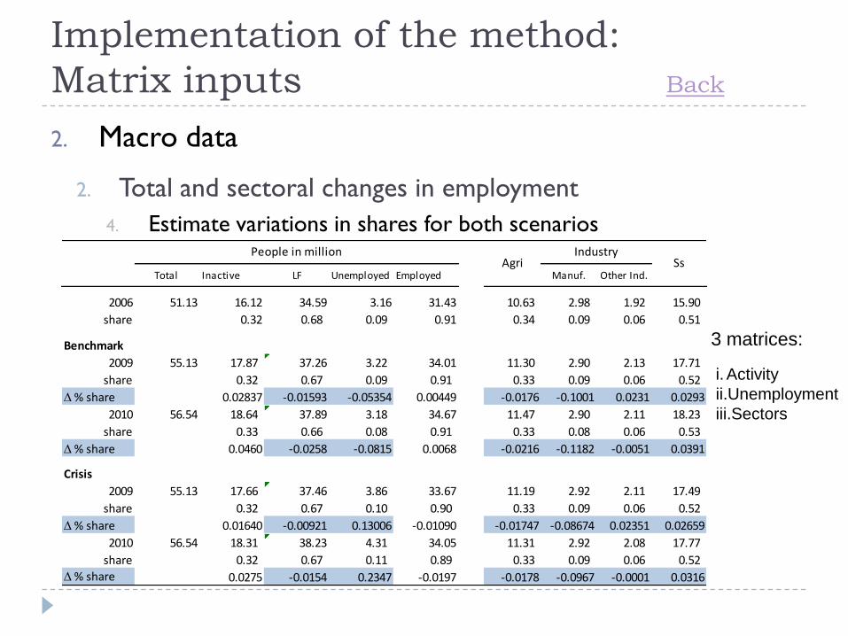
Implementation of the method:
Matrix inputs Back
2. Macro data
2. Total and sectoral changes in employment
4. Estimate variations in shares for both scenarios
Total Inactive LF Unemployed Employed Manuf. Other Ind.
2006 51.13 16.12 34.59 3.16 31.43 10.63 2.98 1.92 15.90
share 0.32 0.68 0.09 0.91 0.34 0.09 0.06 0.51
Benchmark
2009 55.13 17.87 37.26 3.22 34.01 11.30 2.90 2.13 17.71
share 0.32 0.67 0.09 0.91 0.33 0.09 0.06 0.52
D % share 0.02837 -0.01593 -0.05354 0.00449 -0.0176 -0.1001 0.0231 0.0293
2010 56.54 18.64 37.89 3.18 34.67 11.47 2.90 2.11 18.23
share 0.33 0.66 0.08 0.91 0.33 0.08 0.06 0.53
D % share 0.0460 -0.0258 -0.0815 0.0068 -0.0216 -0.1182 -0.0051 0.0391
Crisis
2009 55.13 17.66 37.46 3.86 33.67 11.19 2.92 2.11 17.49
share 0.32 0.67 0.10 0.90 0.33 0.09 0.06 0.52
D % share 0.01640 -0.00921 0.13006 -0.01090 -0.01747 -0.08674 0.02351 0.02659
2010 56.54 18.31 38.23 4.31 34.05 11.31 2.92 2.08 17.77
share 0.32 0.67 0.11 0.89 0.33 0.09 0.06 0.52
D % share 0.0275 -0.0154 0.2347 -0.0197 -0.0178 -0.0967 -0.0001 0.0316
AgriIndustry
SsPeople in million
3 matrices:
i. Activity
ii.Unemployment
iii.Sectors

Implementation of the method:
Matrix inputs
2. Macro data
3. Changes in remittances from abroad
-
10
20
30
40
50
60
70
80
BANGLADESH PHILIPPINES
Labor income Non-labor income Implicit rent
0
10
20
30
40
50
60
70
BANGLADESH PHILIPPINES
Capital Remittances Social Other non-labor
73% Abroad 77 % Abroad
hn
i
J
j
hj
hij
hi
h
h yyIn
y1 1
0
1

Implementation of the method:
Matrix inputs
Changes in remittances from abroad
Remittances in real terms vary depending on changes in the
foreign exchange rate, remittances in nominal terms and
internal inflation
CPI
RR
NR
Δ𝑅𝑅 =
> 0 Δ𝑅𝑁𝜀 > 0
Δ𝐶𝑃𝐼 ≤ 0
= 0 Δ𝑅𝑁𝜀 = Δ𝐶𝑃𝐼
< 0 Δ𝑅𝑁𝜀 ≤ 0Δ𝐶𝑃𝐼 > 0

Implementation of the method:
Matrix inputs
1. Population Growth Projections
2. Macro Data
3. Prices
Why do we need to adjust by prices?
What are the data requirements?

Implementation of the method:
Matrix inputs Back
3. Prices Why do we need to adjust by prices?
Projected incomes or expenditures in real terms adjusted for
spatial differences
Two factors:
1. Poverty line anchored to a fixed basket of food items
2. Food prices move at a different rate than CPI
What are the data requirements?
1. CPI: historical data and projections
2. Weight structure of CPI: food & non-food
3. Weight structure of Poverty line: food & non-food

Implementation of the method:
Micro-data
Why income and not consumption?
Several transmission mechanisms: labor and non-labor market
Poverty on consumption → Map Income into Consumption
Household Income-Generation Model:
1. Labor income: occupational decision & earnings (individual)
2. Non-labor income: remittances, rents, interests, social income
(household level)
hn
i
J
j
hj
hij
hi
h
h yyIn
y1 1
0
1

Implementation of the method:
Micro-data requirements
Main socio-economic variables
1. Household id
2. Demographics: gender, age, relation with household-head
3. Housing & land
4. Education variables
5. Regional variables
6. Labor variables: labor status, labor relation, sector (main and
secondary occupation)
7. Income variables: Labor and Non-labor income
8. Poverty: poverty lines
All income and consumption variables must be adjusted for
spatial/regional price differences
Back
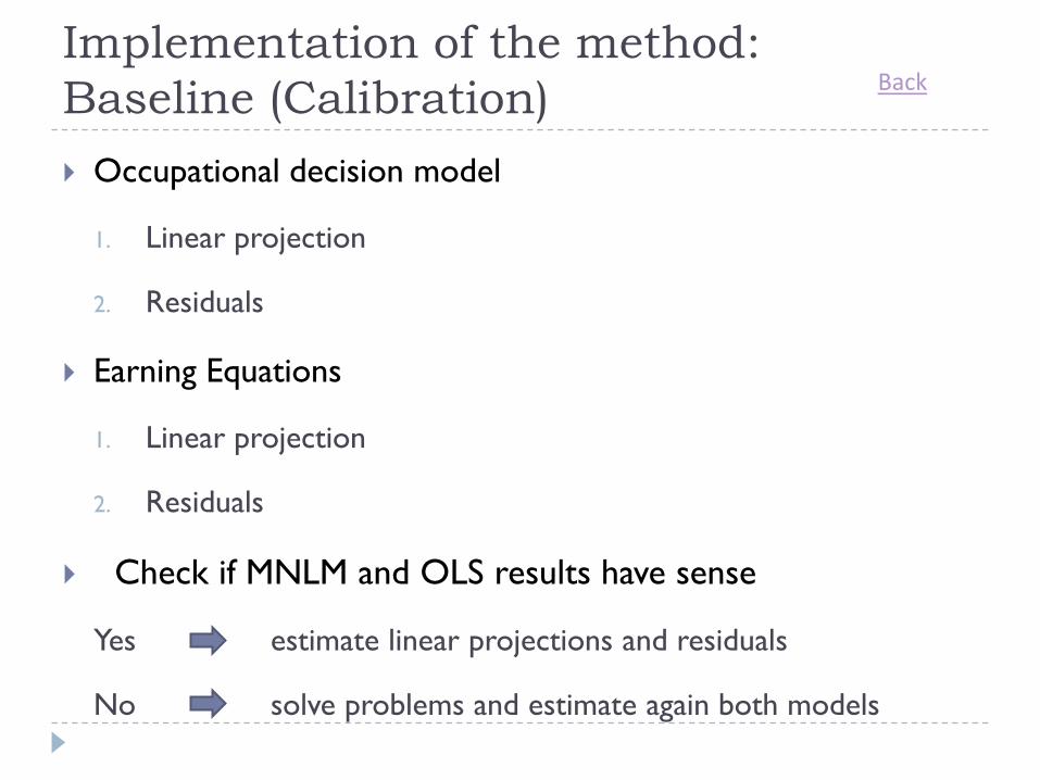
Implementation of the method:
Baseline (Calibration)
Occupational decision model
1. Linear projection
2. Residuals
Earning Equations
1. Linear projection
2. Residuals
Check if MNLM and OLS results have sense
Yes estimate linear projections and residuals
No solve problems and estimate again both models
Back

Results:
Overview of Typical Results
Household income, poverty and inequality
1. Earnings and income impacts
2. Overall poverty and inequality impact
3. Impacts across regions and areas
4. Other analysis: by gender
Distribution analysis
1. A profile of the “crisis-vulnerable”
2. Growth incidence curves
3. Transition matrices
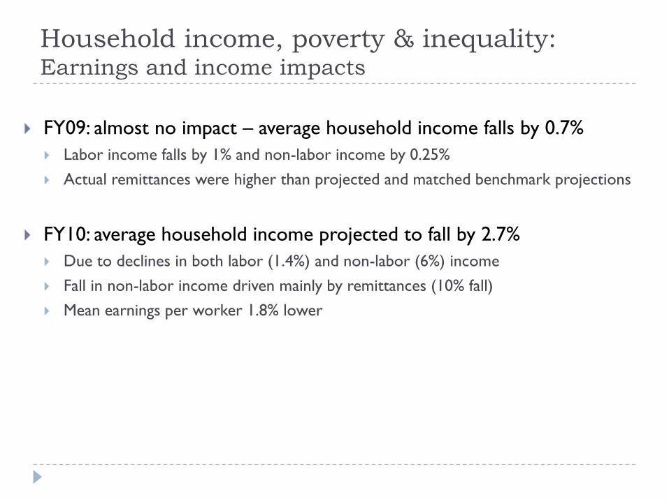
Household income, poverty & inequality: Earnings and income impacts
FY09: almost no impact – average household income falls by 0.7%
Labor income falls by 1% and non-labor income by 0.25%
Actual remittances were higher than projected and matched benchmark projections
FY10: average household income projected to fall by 2.7%
Due to declines in both labor (1.4%) and non-labor (6%) income
Fall in non-labor income driven mainly by remittances (10% fall)
Mean earnings per worker 1.8% lower

Household income, poverty & inequality: Overall poverty and inequality impacts
Comparing hypothetical benchmark (no crisis) and crisis scenarios for FY09 and FY10
FY09: just a slight increase in extreme poverty rate and poverty gap
FY10: 2.3 pct pt increase in poverty rate and 1.4 pct pt increase in extreme poverty rate (~4 million additional people in poverty)
Around 0.5 point increase in poverty gap and 0.1 pt increase in severity
Slight reduction in inequality measures (Gini, Theil indices)
2005Benchmark Crisis
2009 2010 2009 2010
Poverty
-Headcount rate 40.0 32.9 27.6 32.9 29.9
-Poverty gap 9.0 7.4 6.0 7.5 6.5
-Severity of poverty 2.9 2.4 1.9 2.5 2.0
Extreme poverty
-Headcount rate 25.1 20.3 16.8 20.5 18.2
-Poverty gap 4.7 3.9 3.0 3.9 3.3
-Severity of poverty 1.3 1.1 0.9 1.1 0.9
Inequality
-Gini 0.33 0.35 0.35 0.34 0.34
-Theil 0.22 0.23 0.24 0.22 0.22
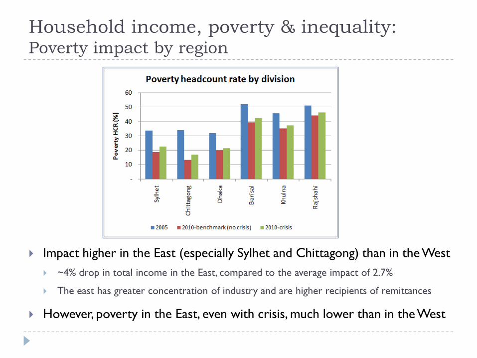
Household income, poverty & inequality: Poverty impact by region
Impact higher in the East (especially Sylhet and Chittagong) than in the West
~4% drop in total income in the East, compared to the average impact of 2.7%
The east has greater concentration of industry and are higher recipients of remittances
However, poverty in the East, even with crisis, much lower than in the West

Distribution analysis:A profile of “crisis-vulnerable”
Question: Households that would not have been poor in 2010 if
had there been NO crisis
How we define our population of analysis:1. Define the poor in benchmark scenario
2. Define the poor in crisis scenario
3. “Vulnerable”: poor in crisis & non-poor in benchmark
4. “Structurally”: poor in crisis & poor in crisis
Poor Non-poor
Poor Structural Vulnerable
Non-poor New rich Never poor
Benchmark
Crisis

Distribution analysis:
A profile of “crisis-vulnerable”
“Crisis vulnerable”: households who are poor with crisis in 2010, but would not be so if there were no crisis
Their characteristics
82% are rural compared to 75% of the general population
Dependency ratio 22% higher compared to the overall population
94% with education 0-9 yrs compared to 75% for general population
Suffer large income losses with a 33% drop in average hhold income
Mostly due to fall in remittances – both no. of receivers and amounts
Even though the direct impact is low in agricultural sector, those vulnerable to becoming poor are mainly in rural areas
Lower incomes in the first place – fall in remittance has large impact

Distribution analysis:Growth incidence curves
Question: Did the crisis impact uniformly the entire distribution?
Growth incidence curve plots the growth rate at each quantile of per
capita income (or expenditure)
The graph can allow us to compare the “impact” of the crisis in poorer
segments of the population with that of richer segments
How you can construct them:
1. Rank the observations by per capita income (or expenditure) from poorest to
richest for benchmark and crisis distributions
2. Calculate quantiles of per capita income (or expenditure) in both scenarios
3. Use the mean income (or expenditure) measure for a given quantile p at two
different scenarios, crisis and benchmark, to calculate the growth rate for
quantile p:
1)(
)()(
2010
2010
py
pypg
b
cc

Distribution analysis:Growth incidence curves
Negative growth in consumption highest from 50th to 90th pctile
Leads to relatively low impact on poverty rate
Raises concerns about distribution and the middle class –beyond absolute poverty
Impact highest among 20th-60th pctile in urban areas, skewed towards
the better off in rural areas
-5.0
0-4
.00
-3.0
0-2
.00
-1.0
00
.00
% C
han
ge
0 10 20 30 40 50 60 70 80 90 100
Percentile
-5.0
0-4
.00
-3.0
0-2
.00
-1.0
00
.00
% C
han
ge
0 10 20 30 40 50 60 70 80 90 100
Percentile
Urban Rural
Per capita Expenditure PCEXP by urban/rural

Distribution analysis:Growth incidence curves
Loss of labor income highest in industry, followed by services
Distributed uniformly in industry, skewed towards the lower earners
in services
-5.0
0-4
.00
-3.0
0-2
.00
-1.0
00.
00
% C
hang
e
0 10 20 30 40 50 60 70 80 90 100
Percentile
Agriculture Industry Services
Labor income by sector

Distribution analysis:Growth incidence curves
Consumption loss higher and more
unevenly distributed in the East
Impact highest for 20th-50th pctile of pcexp
Impact smaller and more evenly distributed
in the West
East-west differences mainly due to
remittances
Not much difference in loss of labor income
But those above 60th percentile lose more
labor income in East than West
-8.0
0-7
.00
-6.0
0-5
.00
-4.0
0-3
.00
-2.0
0-1
.00
0.0
01
.00
2.0
0
% C
han
ge
0 10 20 30 40 50 60 70 80 90 100
Percentile
West: Barisal, Khulna & Rajshahi East: Chittagong, Dhaka & Sylhet
-8.0
0-7
.00
-6.0
0-5
.00
-4.0
0-3
.00
-2.0
0-1
.00
0.0
01
.00
2.0
0
% C
han
ge
0 10 20 30 40 50 60 70 80 90 100
Percentile
West: Barisal, Khulna & Rajshahi East: Chittagong, Dhaka & Sylhet
GIC of per capita labor income
GIC of per capita expenditure

Distribution analysis:Transition matrices
Question: How were the upward and downward household movements’ in
deciles terms?
Transition matrices allow us to look movement of households across the
distribution as a result of a crisis compared to benchmark
How you can build them:
1. Rank the observations by per capita income (or expenditure) from poorest to
richest for benchmark scenario
2. Calculate deciles of per capita income (or expenditure) in benchmark
3. Take each deciles limits
4. Rank the observations by per capita income (or expenditure) from poorest to
richest for crisis scenario
5. Calculate deciles of per capita income (or expenditure) in crisis with deciles
limits benchmark

Distribution analysis:Transition matrices
Deciles defined by benchmark levels household move relative to the “no-crisis” distribution
Most of the “transitions” driven by the fall in non-labor income, mainly remittances
95% of households remain in the same decile for per capita labor income, 70% for per capita total income
Most of the transitions occurs in the middle of the distribution (4th to 8th deciles)
Shift in terms of the distribution of labor income highest for the 7th and 8th deciles
Movements down are larger than movements up for the 4th decile and above
Transition matrices can also be constructed by consumption and for sub-groups

Implications of Results
Identification of main transmission mechanisms to households
In the case of Bangladesh, remittances and food prices were a key determinant of
poverty impact
Identification of possible “leading indicators” to monitor the likely
poverty impact of an economic crisis
E.g. wages, remittance flows
Poverty measures do not capture the full distributional impact
Has implications for targeting of policies and safety nets
Back

Moving forward
Possible extensions, depending on the country context
Commodity price changes
More disaggregated treatment of sectors
More sophisticated treatment of remittances and internal migration
Explicit modeling of demand for skills
Where it can be applied – data requirements
Up-to-date macro projections by sector, with and without crisis; recent
household survey with incomes classified by sector
Even better: surveys (e.g. labor force, rapid monitoring) from 2009, migration info
in household survey
Robustness of results: path dependence analysis and confidence
intervals