assessing distribution, habitat suitability, and site
TRANSCRIPT

i
Assessing Distribution, Habitat Suitability, and Site Occupancy of Great Gray Owls
(Strix nebulosa) in California
By
CARIE L. SEARS
B.S (University of California, Davis) 2002
THESIS
Submitted in partial satisfaction of the requirements for the degree of
MASTER OF SCIENCE
in
Avian Science
in the
OFFICE OF GRADUATE STUDIES
of the
UNIVERSITY OF CALIFORNIA
DAVIS
Approved:
______________________________
______________________________
______________________________
Committee in Charge
2006
ii
Acknowledgements
I would like to thank California Department of Fish and Game, and the University of
California, Wildlife Health Center for their logistical and financial support. Professor
John Eadie provided immense assistance in all aspects of the project, including design
and implementation, statistical and program support, technical review, and logistical and
academic advice. Professors Dan Anderson and Marcel Holyoak offered constructive
comments on project design, treatment, and review. CDFG biologist Chris Stermer and
Kevin O’Connor provided advice and support throughout the study. Essential
cooperation and collaboration was given by the U.S Forest Service and National Park
Service throughout the project duration. Tiffany Manger, Aaron McFadden, Richard
Montgomery, Keri O’Connor, Melissa Odell, Cotton Rockwood, Randy Shields, Todd
Stansbery, Joshua Stumpf, and Ted Woods all provided outstanding assistance in the
field. My lab group, Sharon Gericke, Peter Gilbert, Nicole Kosteczko, Jeremy Kwolek,
Shaun Oldenburger, Matt Wilson, and Greg Yarris, provided friendly support and a
listening ear. Darryl Mackenzie supplied assistance with statistical programs in a time of
great need, and Jeff Maurer provided important comments project design, as well as
assisting in the field. Darca Morgan and Tom Beck acted as an important liaison to the
Forest Service, and John Keane and his crews provided support in the field and
demonstrated a willingness to share ideas throughout the study. Malcolm North provided
constructive advice on habitat sampling. Without the assistance, patience, and
willingness of all these individuals and organizations this project study would have never
proceeded or reached completion.
iii
Table of Contents
List of Tables ___________________________________________________________v
List of Figures _________________________________________________________ vi
List of Appendices _____________________________________________________ vii
Chapter 1 Distribution of Great Gray Owls in California_______________________ 1
1. Introduction_________________________________________________________ 2
2. Methods ____________________________________________________________ 6
2.1 Site Selection for Areas of Known and Unknown Status _______________________ 6
2.2 Survey Protocol_________________________________________________________ 6
3. Results _____________________________________________________________ 9
4. Discussion _________________________________________________________ 10
Tables and Figures_____________________________________________________ 14
Literature Cited _______________________________________________________ 16
Chapter 2 Assessing Habitat Suitability and Site Occupancy of Great Gray Owls
(Strix nebulosa) in California ____________________________________________ 18
1. Introduction________________________________________________________ 19
2. Methods ___________________________________________________________ 23
2.1 Study Area____________________________________________________________ 23
2.2 Survey Protocol________________________________________________________ 23
2.3 Site Sampling _________________________________________________________ 24
2.4 Habitat Variable Sampling ______________________________________________ 25
2.5 Data Analysis _________________________________________________________ 28
2.6 Habitat Suitability Index Field Validation__________________________________ 29
2.7 Site Occupancy Model Design and Selection ________________________________ 29
3. Results ____________________________________________________________ 37
3.1 Habitat Suitability Index Field Validation__________________________________ 37
3.2 Site Occupancy Model __________________________________________________ 37
3.3 Modeling Habitat Variables using Principle Component______________________ 38
3.4 Modeling HSI Values ___________________________________________________ 39
3.5 Contrasting Top Models ________________________________________________ 39
4. Discussion _________________________________________________________ 40
4.1 Habitat Suitability Index Field Validation__________________________________ 40
4.2 Occupancy Models in Assessing Suitable Habitat ____________________________ 42

iv
4.3 Occupancy Models in Estimating Ψ _______________________________________ 45
4.4 Implications of Study ___________________________________________________ 46
Figures and Tables_____________________________________________________ 48
Appendices ___________________________________________________________ 60
Literature Cited _______________________________________________________ 78
v
List of Tables
Table 1.1. Surveys performed across the Sierra Nevada in 2004 and 2005_______15
Table 1. Variables used in HSI calculation and validation___________________52
Table 2. Abbreviations and definitions for continuous and categorical habitat
variables collected at 52 sites across the Sierra Nevada in 2004 and 2005________53
Table 3. Summary of results after application of Beck and Craig HSI model
to sites where surveys and habitat collection was conducted in 2004 and 2005 ___54
Table 4. Site occupancy model and parameter estimation for individual
a priori variables ranked according to Akaike’s Information Criteria corrected
for small sample size and dispersion (QAICc)_______________________________55
Table 5. PC factors eigenvalues, variance contribution of each factor , and
factor grouping descriptions _____________________________________________56
Table 6. Site occupancy model and parameter estimation for PC factors
according to Akaike’s Information Criteria corrected for small sample size and
dispersion (QAICc)_____________________________________________________57
Table 7. Site occupancy model and parameter estimation for HSI values
according to Akaike’s Information Criteria corrected for small sample size and
dispersion (QAICc)_____________________________________________________58
Table 8. Comparison of top site occupancy models for a priori, PC, and HIS
analyses ______________________________________________________________59
vi
List of Figures
Figure 1.1. Map of California indicating 2004 and 2005 great gray owl survey
sites and detections _____________________________________________________14
Figure 1. Map of California indicating 2004 and 2005 habitat assessment sites__48
Figure 2. Diagram of habitat sampling scheme showing meadow and forest
transects______________________________________________________________49
Figure 3. Schematic representation of HSI values and equation relationships___50
Figure 4. Graph of Habitat Suitability Curves of HSI model _________________51

vii
List of Appendices
Appendix A. Correlation matrix for all habitat variables_____________________60
Appendix B. HSI variables, overall HSI value, and survey results for 2004
and 2005______________________________________________________________61
Appendix C. Stacked dot plots of 8 a priori variables showing relationships
between presence and absence in sites inside and outside the core range_________64
Appendix D. Great Gray Owl Survey Protocol Revision Recommendations
Incorporating Detection Probability______________________________________68

1
Chapter 1
Distribution of Great Gray Owls in California

2
1. Introduction
Current knowledge on distribution and total population estimates for the great
gray owl (Strix nebulosa) in California is limited, despite the fact that they have been
listed as State endangered since 1980 (Winter 1980). Estimates have thus far been
speculative given the limited survey effort across the entire Sierra Nevada. In addition,
research is difficult due to the wary and elusive behavior of this species. This fact affects
management and preservation of essential owl habitat throughout its California
distribution.
The distribution of the great gray owl is circumpolar, and the Sierran population
represents the most southern and disjunct in this distribution. Numerous observational
and systematic studies have been conducted across the entire distribution, although
studies on the California population have mainly focused on areas within the core range.
Yosemite National Park, and adjacent areas in Sierra National Forest, and Stanislaus
National Forest make up the core range, and few focused surveys have been conducted
north or south of this area where detections are thought to become irregular.
To date, studies conducted assessing owl numbers have found the population
within the core is relatively small. Winter (1986) estimated 73 individuals in the greater
Yosemite region based on presence of old-growth forest. Greene (1995) provided
estimates of just over 100 for the same region based on potential available habitat.
Within the core range, owls generally exist at elevations between 750 and 2700 meters
(Winter 1980, 1986, Greene 1995).
Great gray owls require two distinct habitat components: (1) a meadow system
with a sufficient prey base, mainly Microtus spp. and Thomomys sp., and (2) an adjacent
forest system able to provide adequate cover and nesting structures (Winter 1980, 1986,
3
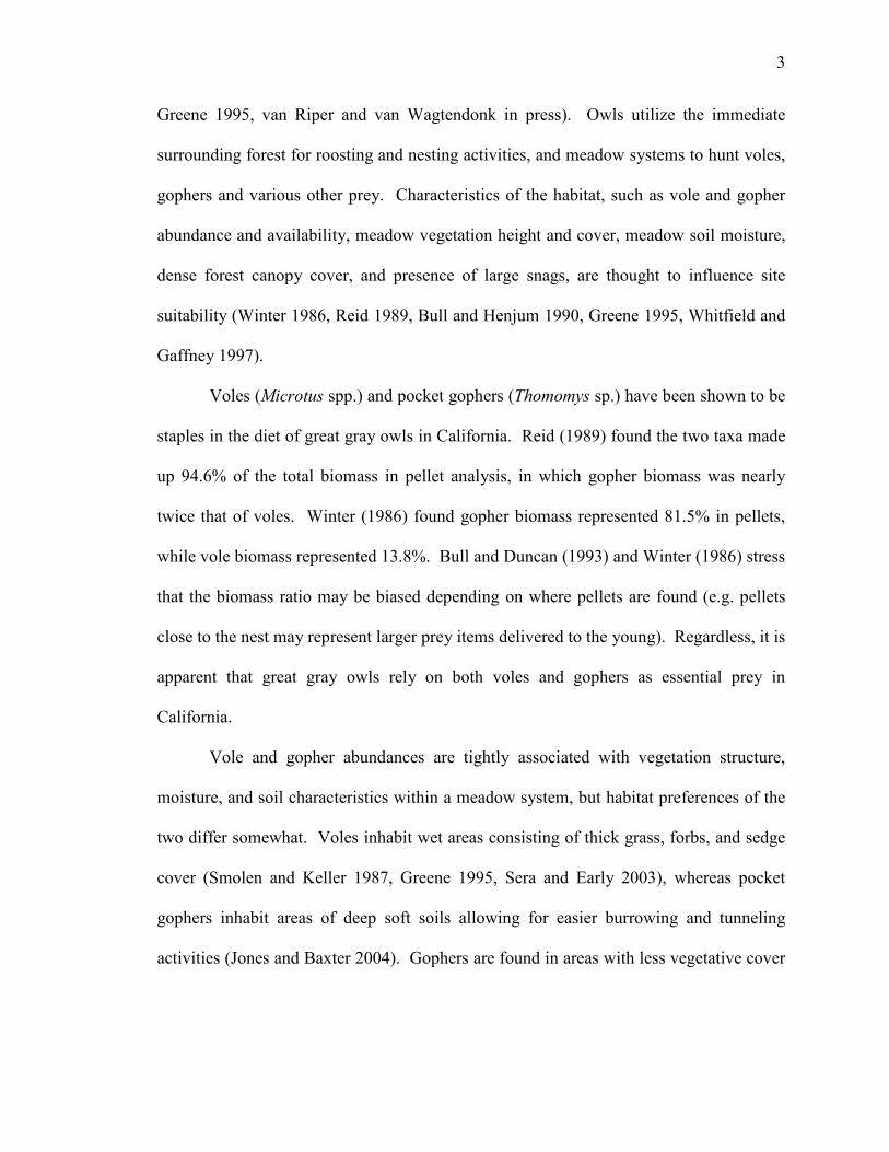
Greene 1995, van Riper and van Wagtendonk in press). Owls utilize the immediate
surrounding forest for roosting and nesting activities, and meadow systems to hunt voles,
gophers and various other prey. Characteristics of the habitat, such as vole and gopher
abundance and availability, meadow vegetation height and cover, meadow soil moisture,
dense forest canopy cover, and presence of large snags, are thought to influence site
suitability (Winter 1986, Reid 1989, Bull and Henjum 1990, Greene 1995, Whitfield and
Gaffney 1997).
Voles (Microtus spp.) and pocket gophers (Thomomys sp.) have been shown to be
staples in the diet of great gray owls in California. Reid (1989) found the two taxa made
up 94.6% of the total biomass in pellet analysis, in which gopher biomass was nearly
twice that of voles. Winter (1986) found gopher biomass represented 81.5% in pellets,
while vole biomass represented 13.8%. Bull and Duncan (1993) and Winter (1986) stress
that the biomass ratio may be biased depending on where pellets are found (e.g. pellets
close to the nest may represent larger prey items delivered to the young). Regardless, it is
apparent that great gray owls rely on both voles and gophers as essential prey in
California.
Vole and gopher abundances are tightly associated with vegetation structure,
moisture, and soil characteristics within a meadow system, but habitat preferences of the
two differ somewhat. Voles inhabit wet areas consisting of thick grass, forbs, and sedge
cover (Smolen and Keller 1987, Greene 1995, Sera and Early 2003), whereas pocket
gophers inhabit areas of deep soft soils allowing for easier burrowing and tunneling
activities (Jones and Baxter 2004). Gophers are found in areas with less vegetative cover
4
than voles, and they also tend to avoid saturated soils due to burrow flooding (Greene
1995, Ingles 1952).
The forest surrounding the meadow system is a critical component because it
offers essential shade for roosting, and structures for nesting. The forest within 200-300
m of the meadow is used for nesting, forest within 10-100 m is used for roosting, and
broken-top snags large enough to support nests are an important factor to facilitate
breeding (Winter 1980, 1986). Greene (1995) also found owl presence to be positively
correlated with montane meadows and high forest canopy closure within the 200 meter
forest buffer surrounding the meadow. Studies outside of California in Oregon and
Canada report similar findings, with the exception of nest type (Bryan and Forsman 1987,
Bull et al. 1988, 1989, Bull and Henjum 1990, Hayward and Verner 1994, Whitfield and
Gaffney 1997). In great gray owl populations outside of California there is preference for
abandoned raptor nests, whereas in California owls mainly use large broken-top snags for
nesting structures (Winter 1980, 1986).
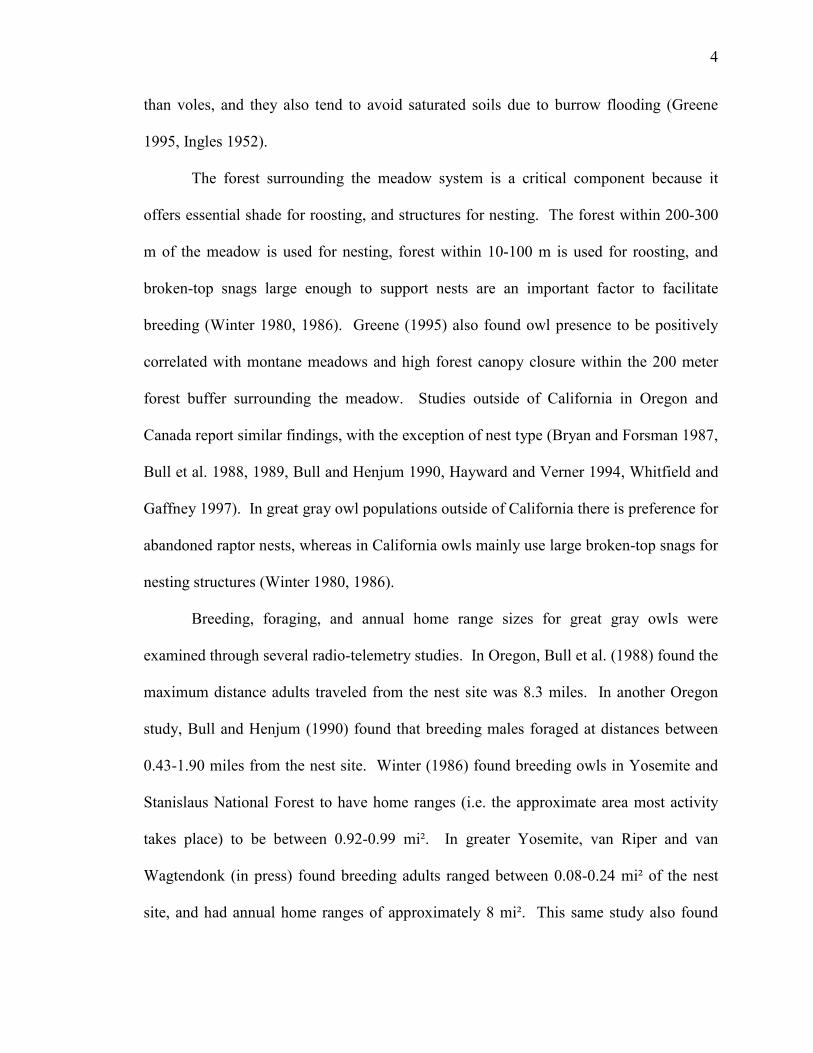
Breeding, foraging, and annual home range sizes for great gray owls were
examined through several radio-telemetry studies. In Oregon, Bull et al. (1988) found the
maximum distance adults traveled from the nest site was 8.3 miles. In another Oregon
study, Bull and Henjum (1990) found that breeding males foraged at distances between
0.43-1.90 miles from the nest site. Winter (1986) found breeding owls in Yosemite and
Stanislaus National Forest to have home ranges (i.e. the approximate area most activity
takes place) to be between 0.92-0.99 mi². In greater Yosemite, van Riper and van
Wagtendonk (in press) found breeding adults ranged between 0.08-0.24 mi² of the nest
site, and had annual home ranges of approximately 8 mi². This same study also found

5
over 60% of all relocations occurred within the 100m forested buffer around meadows,
and 80% occurred within the 200m buffer. These results suggest that ranges vary in
different geographic regions (Oregon vs. California) and different times (breeding vs.
winter). Based on the studies in California, breeding home ranges average between 0.16-
0.99 mi², and most of the owl's time is spent in the 200m forested buffer zone.
The objective of this paper is provide further information on the current
distribution of great gray owls. In addition, this study addresses several objectives of the
California Department of Fish and Game, Resource Assessment Program (RAP). Five
specific RAP goals relate to this work: (1) Acquire baseline information for species and
habitat elements currently not addressed through other monitoring efforts; (2) integrate
monitoring plans across the various biological disciplines; (3) identify important
biological data gaps; (4) investigate how abundance and distribution of species change
due to natural and human-caused factors; and (5) implement an adaptive management
strategy (CDFG). Through promoting an ongoing monitoring for great gray owls within
the Sierra Nevada and extending focused survey efforts outside of the core range, this
study achieves or addresses each of the objectives listed above.
6
2. Methods
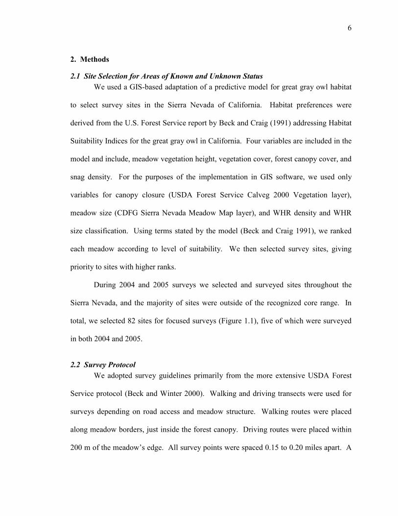
2.1 Site Selection for Areas of Known and Unknown Status
We used a GIS-based adaptation of a predictive model for great gray owl habitat
to select survey sites in the Sierra Nevada of California. Habitat preferences were
derived from the U.S. Forest Service report by Beck and Craig (1991) addressing Habitat
Suitability Indices for the great gray owl in California. Four variables are included in the
model and include, meadow vegetation height, vegetation cover, forest canopy cover, and
snag density. For the purposes of the implementation in GIS software, we used only
variables for canopy closure (USDA Forest Service Calveg 2000 Vegetation layer),
meadow size (CDFG Sierra Nevada Meadow Map layer), and WHR density and WHR
size classification. Using terms stated by the model (Beck and Craig 1991), we ranked
each meadow according to level of suitability. We then selected survey sites, giving
priority to sites with higher ranks.
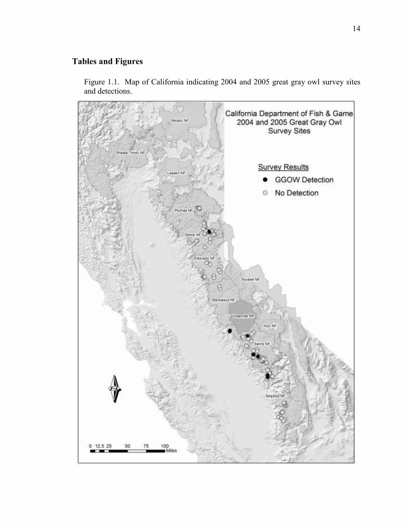
During 2004 and 2005 surveys we selected and surveyed sites throughout the
Sierra Nevada, and the majority of sites were outside of the recognized core range. In
total, we selected 82 sites for focused surveys (Figure 1.1), five of which were surveyed
in both 2004 and 2005.
2.2 Survey Protocol
We adopted survey guidelines primarily from the more extensive USDA Forest
Service protocol (Beck and Winter 2000). Walking and driving transects were used for
surveys depending on road access and meadow structure. Walking routes were placed
along meadow borders, just inside the forest canopy. Driving routes were placed within
200 m of the meadow’s edge. All survey points were spaced 0.15 to 0.20 miles apart. A

7
calling device was used to generate broadcast calls played at each survey point. The
calling sequence at each survey station lasted eight minutes followed by 2 minutes of
quiet listening time.
We conducted two to six visits at each site per year, generally in March to
September. According to Beck and Winter (2000) the most valuable visit is thought to be
during courtship, due to territoriality of the males. Therefore, we made concerted efforts
to conduct two to three nighttime visits during the early nesting season (courtship and
incubation periods), occurring from sunset to 1 or 2 am. Generally, one to two nighttime
visits took place within the late nesting season (brooding and post-fledge periods),
occurring 2 hours before sunset lasting through 2-4 hours past sunset. At most sites we
conducted a final visit during the day as a meadow search. During this time the
surveyor(s) searched for molted feathers, regurgitated pellets, whitewash on snags and
under roost sites, foraging perches within or near the meadow, and visual or auditory
detection of an owl. A positive identification was confirmed only by visual or audio
detection, or the presence of feathers.
If an owl vocally responded at any point, the surveyors recorded a compass
bearing and estimated the distance to source. A follow-up visit was then performed
during daylight hours near the estimated source to investigate further occupancy status
within 48 hours of the original response. During the follow-up visit, the surveyors looked
for molted feathers, regurgitated pellets, whitewash on snags and under roost sites, or
visual/audio detection of an owl. The search continued in this manner for 2 hours or until
owl(s) were located and/or occupancy status confirmed.

8
In 2004 we attempted to make six visits per site, and in 2005 the goal was to make
at least four visits per site. Both years had an unusually high snow-load and late melt-off
date making access problematic, particularly so in 2005. Ultimately, limited access to
sites decreased the number of surveys conducted over both years. Sites received on
average four to six visits per year (2-6 visits/site/year) with a higher concentration of
visits later in the season.
9
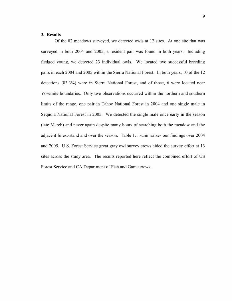
3. Results
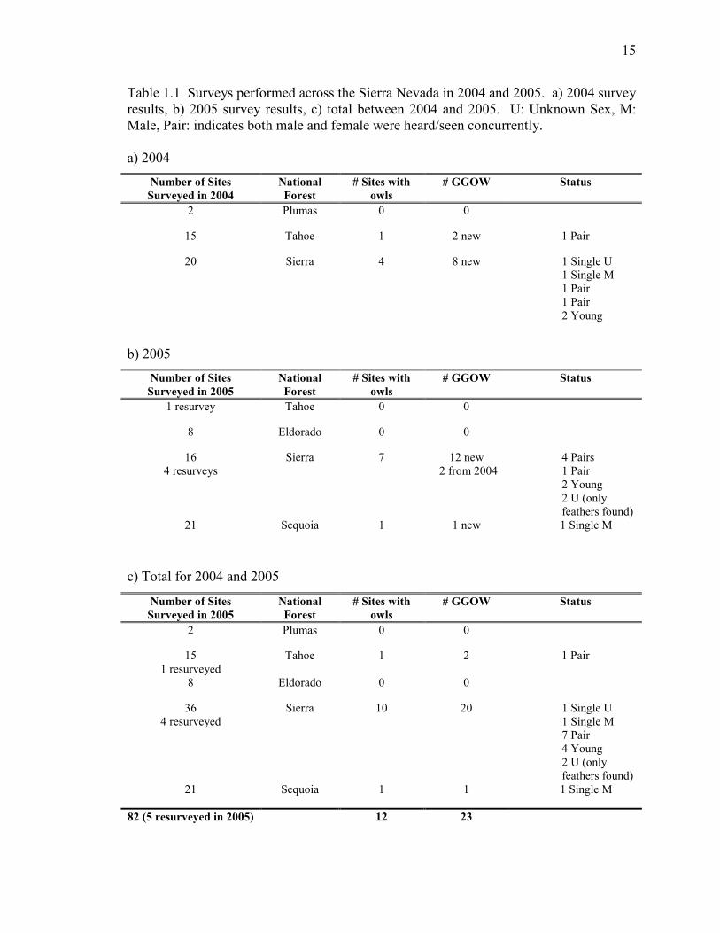
Of the 82 meadows surveyed, we detected owls at 12 sites. At one site that was
surveyed in both 2004 and 2005, a resident pair was found in both years. Including
fledged young, we detected 23 individual owls. We located two successful breeding
pairs in each 2004 and 2005 within the Sierra National Forest. In both years, 10 of the 12
detections (83.3%) were in Sierra National Forest, and of those, 6 were located near
Yosemite boundaries. Only two observations occurred within the northern and southern
limits of the range, one pair in Tahoe National Forest in 2004 and one single male in
Sequoia National Forest in 2005. We detected the single male once early in the season
(late March) and never again despite many hours of searching both the meadow and the
adjacent forest-stand and over the season. Table 1.1 summarizes our findings over 2004
and 2005. U.S. Forest Service great gray owl survey crews aided the survey effort at 13
sites across the study area. The results reported here reflect the combined effort of US
Forest Service and CA Department of Fish and Game crews.

10
4. Discussion
One goal of this study was to shed light on great gray owl distribution throughout
California. Detections dropped considerably in areas farther from the greater Yosemite
region. Most of the detections were in Sierra National Forest; although this area
represents a greater proportion of total sites surveyed in both 2004 and 2005 (41 out of 82
sites surveyed were in Sierra National Forest). Sections of Sierra National Forest that
border Yosemite are considered in the core area for the species. There is a small
population near Shaver Lake and Dinkey Creek area in Sierra National Forest, located
approximately 90 to100 miles south-southeast of Yosemite. Survey records for this area
are consistent since 1989, suggesting a relatively stable population.
Survey records for the southern Sierra Nevada show great gray owl territories
centered near Sequoia National Park dating between 1988 and 2001. Our surveys in this
area were unsuccessful at locating any owls. However, we did not survey inside of
Sequoia National Park and it is likely that occupied sites are still dispersed in that area. A
focused survey effort is needed to confirm population status within Sequoia National
Park and the surrounding areas.
Only two detections were obtained in the extremities of the northern and southern
Sierra: a pair in Tahoe National Forest detected several times in 2004 but not in 2005,
and a single male in southern Sequoia National Forest detected once in 2005. The site in
Sequoia National Forest was at low elevation (4500 ft.) and early in the season (March);
therefore it is probable the single male was a floater awaiting access to higher elevation
sites, or a disperser seeking a suitable territory. Floaters are typical for great gray owls in
the winter as they tend to move down-slope when high snow load prevents foraging and
11
as young search for suitable unoccupied territories (Bull and Duncan 1993). Moreover, a
large herd of cattle (over 100 head) grazed this site in April, which quickly degraded
meadow structure and made it unsuitable for both owls and prey. In addition to our
surveys, a private consulting firm conducting surveys in Plumas National Forest
(northern Sierra) found a great gray owl pair at a site in both 2004 and 2005. These
detections are the most recent confirmed record for great gray owls in the northern region
of California.
The second objective of this study was to explore current population numbers of
great gray owls throughout the Sierra. Our survey results, in combination with the pair
detected in Plumas National Forest, add to earlier estimates by establishing presence at 12
additional sites across the Sierra Nevada, totaling 23 individuals (Table 1.1). This
increases the estimate to approximately 123 individuals across the Sierra Nevada,
assuming earlier estimates are relatively static. However, many sites throughout the
Sierra still remain unsurveyed making reasonable inferences about great gray owl
numbers in California difficult. In addition, the Habitat Suitability Model used to select
sites is not completely accurate, as shown in the following chapter, and therefore sites
occupied by great gray owls may not have been captured in this study.
Several factors may have affected owl occupancy during this study. Both years
produced high snow loads, although the snow-load in 2005 was particularly long lasting.
Access to high elevation sites was difficult because of snow cover, and some sites
remained under snow through late-June. Late-season snow conditions in the Sierras are
usually icy and hard-packed, making foraging difficult for owls. In addition, it is
possible that vole populations were experiencing a natural cyclic low during this study,
12
which can perpetuate low occupancy and reproductive rates at sites otherwise suitable.
To overcome such complexities, a long-term monitoring effort to determine occupancy
and examine demography for the species is clearly needed for the California population.
Our surveys suggest that great gray owl populations are somewhat constrained to
the greater Yosemite area, although the reasons for this remain unclear. It is possible
northern and southern areas have consistently experienced low or irregular great gray owl
numbers due to large distances from core population, and/or marginal habitat unable to
sustain breeding owls. Other factors affecting north-south expansion may include habitat
degradation via human disturbance (grazing, logging, and development), differences in
regional cyclic prey abundances, and/or an overall decrease in great gray owl numbers
Sierra-wide.
We conclude that the great gray owl distribution extends throughout the Sierra
Nevada; however, greater densities occur in the central region including Stanislaus and
Sierra National Forests and Yosemite National Park. As Winter (1986) suggests, the
opportunity for range expansion exists within the Sierra, however unknown factor(s) may
limit dispersal and population stability outside of the core range. Population estimates
throughout the Sierra are steadily increasing as more surveys are conducted.
Nevertheless, numbers are still low compared to the large area of potential habitat the
Sierra Nevada offers. These small populations are extremely sensitive to disturbance,
habitat degradation, climate change, pollution, and disease and, for this reason, continued
monitoring and research is critical to ensure the sustainability of California’s great gray
owl population(s).

13
During this study we began to fill essential data gaps for this species. Information
on great gray owl distribution and population numbers was expanded by means of an
initial monitoring effort. Further research investigating key habitat components and
factors relating to site occupancy are the next steps to broaden our knowledge and
facilitate better management decisions.
14
Tables and Figures
Figure 1.1. Map of California indicating 2004 and 2005 great gray owl survey sites
and detections.
15
Table 1.1 Surveys performed across the Sierra Nevada in 2004 and 2005. a) 2004 survey
results, b) 2005 survey results, c) total between 2004 and 2005. U: Unknown Sex, M:
Male, Pair: indicates both male and female were heard/seen concurrently.
a) 2004
Number of Sites
Surveyed in 2004
National
Forest
# Sites with
owls
# GGOW Status
2 Plumas 0 0
15 Tahoe 1 2 new 1 Pair
20 Sierra 4 8 new 1 Single U
1 Single M
1 Pair
1 Pair
2 Young
b) 2005
Number of Sites
Surveyed in 2005
National
Forest
# Sites with
owls
# GGOW Status
1 resurvey Tahoe 0 0
8 Eldorado 0 0
16
4 resurveys
Sierra 7 12 new
2 from 2004
4 Pairs
1 Pair
2 Young
2 U (only
feathers found)
21 Sequoia 1 1 new 1 Single M
c) Total for 2004 and 2005
Number of Sites
Surveyed in 2005
National
Forest
# Sites with
owls
# GGOW Status
2 Plumas 0 0
15
1 resurveyed
Tahoe 1 2 1 Pair
8 Eldorado 0 0
36
4 resurveyed
Sierra 10 20 1 Single U
1 Single M
7 Pair
4 Young
2 U (only
feathers found)
21 Sequoia 1 1 1 Single M
82 (5 resurveyed in 2005) 12 23
16
Literature Cited
Beck, T.W., D.L. Craig. 1991. Habitat Suitability Index and Management
Prescription for the Great Gray Owl in California. USDA Forest Service,
Technical Report (Draft).
Beck, T.W., and J. Winter. 2000. Survey Protocol for the Great Gray Owl in
the Sierra Nevada of California. USDA Forest Service, Pacific Southwest
Region, Vallejo, CA.
Bryan, T, and E.D. Forsman. 1987. Distribution, Abundance, and Habitat of Great Gray
Owls in Southcentral Oregon. The Murrelet. 68: 45-49.
Bull, E.L., and J.R. Duncan. 1993. Great Gray Owl (Strix nebulosa). The Birds of
North America. 41:1-15.
Bull, E.L, and M.G. Henjum. 1990. Ecology of the great gray owl. Gen. Tech Rep.
PNW-GTR-265. Portland, OR: U.S. Department of Agriculture, Forest Service,
Pacific Northwest Research Station. 39 p.
Bull, E.L., M.G. Henjum, R.S. Rohweder. 1988. Nesting and Foraging Habitat of Great
Gray Owls. Journal of Raptor Research. 22: 107-115
Bull, E.L., M.G. Henjum, and R.S. Rohweder. 1989. Diet and Optimal Foraging of
Great Gray Owls. Journal of Wildlife Management. 53: 47-50.
Greene, C. 1995. Habitat Requirements of Great Gray Owls in the Central
Sierra Nevada. M.S. Thesis. University of Michigan, MI.
Hayward, G.D. ed., and J. Verner ed. 1994. Flammulated, Boreal, and Great Gray Owls
in the United States: A Technical Conservation Assessment. USDA GTR-RM-
253.
Ingles, L.G. 1952. The ecology of the mountain pocket gopher, Thomomys monticola.
Ecology. 88: 87-95.
Jones, C.A., and C.N. Baxter. 2004. Thomomys bottae. Mammalian Species. 742: 1-14
Reid, M.E.. 1989. The Predator-Prey Relationship of the Great Gray Owl in Yosemite
National Park. Cooperative National Park Resources Studies Unit, Technical
Report No. 34.
Sera, W.E., and C.N. Early. 2003. Mircrotus montanus. Mammalian Species. No.716,
pp.1-10.
17
Smolen, M.J., and B.L. Keller. 1987. Microtus longicaudus. Mammalian Species. 271:
1-7
van Riper, C., and J.W. van Wagtendonk. Home Range characteristics of great gray
owls in Yosemite National Park. (in press).
Whitfield, M.B., and M. Gaffney. 1997. Great Gray Owl (Strix nebulosa) Breeding
Habitat Use Within Altered Forest Landscapes. Biology and Conservation of
Owls of the Northern Hemisphere. USDA GTR-NC-190. p498-505
Winter, J. 1980. Status and Distribution of the Great Gray Owl in California. State
of California Resources Agency, Department of Fish and Game.
Winter, J. 1986. Status, distribution and ecology of the Great Gray Owl (Strix nebulosa)
in California. M.S. Thesis, San Francisco State University, CA.

18
Chapter 2
Assessing Habitat Suitability and Site Occupancy of Great Gray Owls
(Strix nebulosa) in California
19
1. Introduction
The great gray owl (Strix nebulosa) is one of the most elusive owls found within
the Sierra Nevada mountain range. The distribution of the great gray owl is circumpolar,
and the Sierran population represents the most southern in its range. The Californian
population was listed as endangered in 1980 due to population declines (Winter 1980).
Since then, studies on the California population have focused on the greater Yosemite
region (inclusive of areas outside the park in Stanislaus and Sierra National Forests),
although numerous observational and systematic studies have been conducted across the
entire distribution.
As reported in Chapter 1, studies in California’s Sierra Nevada range over the last
25+ years indicate that great gray owls require two distinct habitat components: 1) a
meadow system that supports voles (Microtus spp.) and gophers (Thomomys sp.), the
preferred prey for great gray owls (Winter 1980, 1986, Greene 1995), and 2) an adjacent
forest system to provide adequate roosting cover and nesting structures (Winter 1980,
1986, Greene 1995, van Riper and van Wagtendonk in press). Since owls utilize the
forest for roosting and nesting activities and meadow systems to hunt prey, characteristics
of this habitat become important in assessing suitability, use, and long-term occupancy.
Studies performed across North America have shown certain key characteristics, such as
vole and gopher abundance and availability, meadow vegetation height and cover,
meadow soil moisture, forest canopy cover, and presence of large snags, influence site
suitability (Winter 1986, Reid 1989, Bull and Henjum 1990, Greene 1995, Whitfield and
Gaffney 1997).
One of the more traditional methods to predict habitat is through Habitat
Suitability Index (HSI) models. These models are developed to aid in management of
20
species through synthesis of information on specific habitat requirements and subsequent
prediction of suitable habitat based on these attributes (Piorecky et al. 1999). The USDA
Forest service developed such a model for great gray owls in California (Beck and Craig
1991). The model is based on a small sample of sites in prime habitat of Yosemite and
integrates known habitat attributes to create a method to predict suitable habitat for great
gray owls throughout the Sierra Nevada. Information on great gray owl requirements for
areas outside the core range was sparse at the time of HSI model development.
Accordingly, Beck and Craig (1991) state “this model is based on limited information for
the Sierra Nevada and should be regarded as preliminary.” Given the historic and
somewhat restrictive nature of the present model, representation of suitable habitat may
be unreliable for the species throughout the entire Sierra Nevada.
A number of approaches have been used to assess the effects of false negative
errors (i.e. recording a species as absent when it is actually present) on wildlife-habitat
relationships, parameter estimates, site occupancy, and population estimates and trends,
including logistic regression, discriminant function analysis, zero-inflated binomial
models, and General Linear Models (Azuma et al. 1990, Stauffer et al. 2002, Tyre et al.
2003, Gu and Swihart 2004, Defos du Rau et al. 2005, Field et al. 2005).
Recently, considerable effort has been directed at ways of estimating abundance
and distribution while accounting for imperfect detection rates among species through the
use of occupancy modeling. Mackenzie et al. (2002) developed a formalized method to
estimate the proportion of sites occupied by a species while accounting for imperfect
detection probabilities (e.g. the probability of detecting a species, if present, is less than
one). These methods utilize maximum likelihood functions to estimate occupancy and

21
detection probability. The model can incorporate covariates to assess the effects of
habitat variables on both occupancy and detection probability. Such a model can provide
important insight into the distribution, proportion of area occupied (e.g. abundance), and
habitat requirements of a species (e.g. suitability), and can help to refine survey protocols
and allocation of effort.
Several recent studies have illustrated the utility of this approach. Ball et al.
(2005) used occupancy models to determine the distribution and habitat requirements of
the Palm Springs ground squirrel (Spermophilus tereticaudus chlorus), and assess the
effectiveness of current management plans. Finley et al. (2005) used occupancy models
to evaluate the importance short grass prairie on occupancy and detection probabilities
for the threatened swift fox (Vulpes velox). Another study on foxes (V. vulpes) used the
model to estimate detection probabilities, and thus maximize survey efficiency (Field et
al. 2005). Wintle et al. (2005) estimated detection probability to evaluate survey effort
allocation for two species of forest owls and four species of marsupials. The effect of
barred owl (Strix varia) presence on northern spotted owl (S. occidentalis caurina)
occupancy and detection probability was assessed by Olson et al. (2005). Occupancy
models were also used for various anuran species to assess the effects of habitat variables
and abundance on occupancy rates and detection probabilities, effectiveness of survey
protocol, and species distribution (Schmidt and Pellet 2005, Pellet and Schmidt 2005).
Bailey et al. (2004) similarly explored the effects of survey method and effort, sampling
variables (i.e. duration of survey), and habitat variables on occupancy and detection
probabilities for terrestrial salamanders.

22
In the present study we evaluate the ability of several analytical approaches to
designate key habitat components related to great gray owl presence across the Sierra
Nevada of California. We also develop functional site occupancy models to estimate the
proportion of suitable area occupied by great gray owls in the Sierra. The long-term
benefits of this project will include a refined understanding of great gray owl habitat
requirements throughout its entire California range, demonstrate an application of a
current modeling approach, and help to refine management efforts for the species.

23
2. Methods
2.1 Study Area
We collected survey and habitat data in the Sierra Nevada mountain range in
California in areas across its entire expanse, including sites in Plumas, Tahoe, Eldorado,
Sierra, and Sequoia National Forests, and Yosemite National Park. All sites were
surveyed by CDFG crews with the exception of those within Yosemite National Park.
Yosemite sites were surveyed by a NPS biologist and Forest Service crew in 2005. All
surveys followed the same protocol and are therefore comparable in nature.
2.2 Survey Protocol
Survey guidelines were adopted from the more extensive USDA Forest Service
protocol (Beck and Winter 2000). All survey points were spaced 240-320 m (0.15 to
0.20 mi) apart at the meadows edge or within the 200 meter forested buffer zone
surrounding each meadow. A calling device was used to generate broadcast calls played
at each survey point. The calling sequence at each survey station lasted eight minutes
followed by two minutes of quiet listening time.
Each site was visited up to six times per year. Visits were timed to the breeding
season which generally lasted March through September depending on region and
elevation. According to Beck and Winter (2000) the most essential visit is thought to be
during courtship, when males are most territorial. Therefore, we undertook strong efforts
to conduct two to three nighttime visits during the early nesting season (courtship and
incubation periods). In addition, we conducted one to two nighttime visits within the late
nesting season (brooding and post-fledge periods). Our final visit was conducted during
the day to search for molted feathers, regurgitated pellets, whitewash on snags and under

24
roost sites, foraging perches within or near the meadow, or visual detection of an owl. A
positive detection was confirmed only by visual or audio detection, or the presence of
feathers.
2.3 Site Sampling
Previous studies to monitor great gray owls have been limited to portions of
Stanislaus and Sierra National Forests, and Yosemite National Park. We surveyed both
sites with historical use by great gray owls and sites where use by great gray owls was
unknown. In total, 60 sites were surveyed for owls and sampled for habitat components
in 2004 and 2005. Sixteen sites were sampled within the core range, and 44 were
sampled outside of that range (including known and unknown occupancy status) (Figure
1). We selected 26 sites with historic use across the Sierra Nevada, of which 10 were
outside the core and 16 were inside the core. Thirty-four sites were selected with
unknown status, of which all were outside the core range.
We utilized knowledge of great gray owl habitat preferences to produce a GIS-
based habitat suitability model, which was then used to select survey sites in the Sierra
Nevada of California outside the owl’s core range. Habitat preferences were derived
partially from the Habitat Suitability Index (HSI) model and management prescription for
the Great Gray Owl in California (Beck and Craig 1991), and partially on habitat
requirements known from the past research in California (Winter 1986, Greene 1995).
The HSI model was designed to predict habitat that is “comprised of mature or old-
growth conifer forests with dense canopy and numerous snags in close proximity to large
meadows or meadow systems” (Beck and Craig 1991). Based on a portion of the HSI
model criteria and known habitat preferences, we used variables for canopy closure
25
(USDA Forest Service Calveg 2000 Vegetation layer), meadow size (CDFG Sierra
Nevada Meadow Map layer), and Wildlife Habitat Relationship System (WHR) density
and size classification in GIS software to rank each meadow according to level of
suitability. We then selected sites representative of all status types for owls (i.e. known,
unknown, and historic), giving priority to sites with higher suitability ranks.
It was necessary to compare areas outside the core to those inside, and to increase
the sample size. Therefore we targeted 11 additional sites inside the core range in 2005
to include in the analysis. Sites within the core range have been monitored extensively
over time and there is either a historic (i.e. records show owl detections at some point in
the past) or current (i.e. owls have been currently detected at site) record for all the sites
selected at the start of the surveys in 2005. When we selected the 11 sites in the core
range, 8 were known to have current great gray owl presence and 3 were known to have
historic records but presence was not currently noted for that year. By the end of the
season, all but one of the 11 sites had documented owl presence.
2.4 Habitat Variable Sampling
Previous analyses have shown strong positive relationships between several
habitat components and great gray owl presence. These include prey abundance, mainly
voles (Microtus spp.) and pocket gophers (Thomomys sp.), and meadow characteristics
that influence the presence of these prey species, such as medium-tall vegetation height,
high vegetation cover, and high soil moisture (Ingles 1952, Rhodes and Richmond 1985,
Winter 1986, Smolen and Keller 1987, Reid 1989, Greene 1995, and Sera and Early
2003). The forest within 100-200 m of the meadows edge is used for nesting and
roosting activities (Winter 1980, 1986, van Riper and van Wagtendonk in press). Within

26
this buffer, forest stand components such as dense forest canopy cover used for shade,
amount of fir (Pseudotsuga spp.), presence of large snags suitable for nesting structures,
are important factors for assessing suitability (Winter 1986, Bryan and Forsman 1987,
Bull et al. 1988, Bull et al. 1989, Reid 1989, Bull and Henjum 1990, Hayward and Verner
1994, Greene 1995, Whitfield and Gaffney 1997, and Fetz et al. 2003).
During the 2004 and 2005 field seasons, we measured variables representing these
documented habitat requirements (Table 2). We placed random transects both in the
meadow and adjacent forest at each site to measure related habitat values such as prey
sign, meadow vegetation traits, forest stand structure, and snag density (Figure 2). To
ensure consistency of data collection we followed methods used by Greene (1995),
Winter (1986), and CNPS Releve Protocol (2003).
Based on these data, we collected habitat data on key meadow components such
as average vegetation height, percent ground cover, meadow moisture, and dominant
vegetation type. In addition, we calculated snag density and percent forest cover within
the 200 meter forested buffer zone surrounding each meadow.
We used randomly placed line transects to measure meadow components at
equally spaced points (10 m) along the transect using a 1x1 m frame with 16 intersections
of 8 crosshairs (four by two). Each transect started at the edge of the meadow and
followed an arbitrary bearing. The frame’s right-hand corner was positioned at each data
point along the transect where we estimated vegetation height, percent ground cover, and
dominant vegetation. We estimated vegetation height by measuring the height of the
tallest vegetation at each crosshair intersection in 2004, and measuring the height of the
tallest vegetation at each corner of the frame in 2005. We estimated percent ground

27
cover by counting the number of crosshairs directly over live or dead-rooted vegetation.
We estimated meadow moisture at each point by labeling as dry, moist, saturated, or
standing water after a visual inspection and depression of the soil within the 1x1 m frame.
Lastly, we classified dominant vegetation as grass, sedge, rush, forbs, shrub, or unknown
within the 1x1 m frame at each data point. We continued in this manner until 50 data
points were collected at each site.
Prey signs were also noted along the same random line transects at equally spaced
points (30 m in 2004 and 20 m in 2005) within the meadow. At these data plots we noted
number of vole runways, gopher mounds, and gopher plugs, and the presence of clippings
and feces, within a 1 m radius of right hand corner of 1x1 m frame. We continued in this
manner until 20 (2004) or 25 (2005) data points were collected at each site.
Some sites consisted of several small meadows in close proximity to each other.
In these cases a portion of the vegetation and prey plots were assigned to each. For
example, if a site contained 3 meadow of size ratio 10:9:5 acres, then 20:20:10 vegetation
plots and 10:10:5 prey plots were performed in each one respectively.
We placed three to five random belt transects within the 200 m forested buffer
running perpendicular to and starting at the meadow’s edge, where the number of
transects depended on meadow size (Figure 2). The belt transects were 210 m in length
and 20 m wide, and five data points were spaced every 40 m along the transect.
We measured forest canopy closure using a spherical densiometer at each of the
five data points within each transect. Four readings, one in each cardinal direction, were
taken and then averaged to obtain a final reading for that point. We measured tree
species and tree diameter at breast height (DBH) using DBH -tape on live trees within a

28
10 m radius of every 40 m data point. In 2004 we measured all trees greater or equal to 5
in DBH, and in 2005 we reduced measurements to all trees greater or equal to 18 in DBH
for the sake of time.
Great gray owls in California mainly use large broken-top snags for nesting
structures (Winter 1980, 1986), therefore we measured snags over 5 in DBH within a 10
m radius of every 40 m data point (species noted if possible). We calculated the area
where snags were measured to obtain a snag density index value (snags per hectare) for
each site.
Meadow size was obtained from a digital polygon meadow layer provided by
California Department of Fish and Game (CDFG). During a general meadow assessment
in accordance with the CDFG Sierra Meadow Project, we performed a visual inspection
for evidence or presence of cattle at each site in both 2004 and 2005.
2.5 Data Analysis
We first implemented the Habitat Suitability Index model (Beck and Craig 1991)
to provide a means of field-validation. We used correlation matrices to examine
relationships among habitat variables. We also used Principle Components Analysis to
reduce the number of variables to a manageable size for further analyses. Finally, we
used site occupancy modeling to estimate occupancy and to assess the influence of
habitat components. We constructed 3 sets of occupancy models using: (1) Individual a
priori habitat variables for 52 sites inside and outside the core; (2) PC factors for 52 sites
inside and outside the core; (3) HSI values for 52 sites inside and outside the core; and 4)
comparative occupancy models using covariates from the top models produced by each
29
of the above analyses. The final results of these models were then used to compare
techniques related to HSI, PCA, and Occupancy modeling.
2.6 Habitat Suitability Index Field Validation
Beck and Craig’s (1991) HSI model is based on four variables representing a
cover/reproductive component (i.e. factors relating to reproductive suitability, such as
snags greater or equal to 24 inch DBH and percent tree canopy closure) and a food
component (i.e. factors relating to prey presence, such as herbaceous height between 13-
38 cm and percent herbaceous cover). These values are then combined to produce an
overall HSI value for each site (Figure 3). HSI values range between zero and one, where
values closer to 1 are considered more suitable then values closer to 0.
To evaluate the predictive ability of Beck and Craig’s (1991) model we used the
model structure to calculate habitat suitability values for our sites. We formatted our
habitat data to fit the variable criteria of the model. For example, V1 is defined as snags
per hectare greater or equal to 24 in DBH. In the habitat dataset, we included the number
of snags meeting this criterion and excluded all snags that did not. We then calculated
the value for each site based on slope of the suitability index curves of the model (Figure
4). Descriptions for each variable, limits, and equations used to calculate values, and the
actions taken to integrate the habitat dataset are shown in Table 1. Sites were then
evaluated based on predicted suitability by comparing the survey results with the HSI
value, where high values equate to high suitability.
2.7 Site Occupancy Model Design and Selection
Using the 2004 and 2005 survey data, we developed a single-season, single-
species site occupancy model for great gray owls in California. The model was designed
30
to estimate the proportion of sites occupied in an area of interest, Ψ, while accounting for
detection probability, p (Mackenzie et al. 2002, 2006). These estimates account for a
species with detection probabilities less than one (e.g. present but not detected; false-
negative surveys).
Briefly, the occupancy model is fashioned after mark-recapture closed population
models, as it assigns encounter histories based on survey visits (MacKenzie et al. 2002).
For example, if a site has six survey visits over a season, and has detections during the 2nd
and 5th visits, the encounter history is written as h = 010010. The model likelihood
equation for this history would then be,
L(Ψ, p) = Ψ(1-p1)p2(1-p3)(1-p4)p5(1-p6) (1)
In this manner, when a species is detected at least once during an encounter history it is
possible to calculate estimations for Ψ and p. The model requires at least two surveys per
site during a survey season, where a species is known to be using a defined area, often
during a breeding season.
Occupancy models are effective at integrating covariate information that may
influence Ψ and p. These parameters can be described as varying or constant over time.
Covariates for Ψ are those that remain constant throughout the survey season, such as
elevation or forest structure. Covariates for p can also be constant over time, but
typically vary over the survey season (e.g. temperature during each visit or duration of
visit). Each covariate can be incorporated into the model through use of logistic
regression, and can then be assessed for covariate effects on occupancy and detection.
31
Due to logistic and fiscal constraints, six visits were not possible at all sites over
the two-year monitoring period. However, the occupancy model is able to accommodate
missing observations. In this case, the missing observation is omitted from the model
likelihood equation and bears no weight in parameter estimation.
For interpretation of the resulting models to be valid it is important to assess how
the model of interest fits the observed data (Cooch and White 2005, MacKenzie et al.
2006). As recommended by MacKenzie et al. (2004) we assessed goodness-of-fit to the
global model (most complex model with the greatest number of parameters) using
bootstrapped chi-square.
There are several assumptions of the model: (1) occupancy at each site should not
change over the survey period; that is sites are closed to changes in occupancy over the
season; (2) probability of occupancy should be constant across sites, or the differences in
occupancy are accounted for by including measured covariates in the model; (3) the
probability of detection should be constant across all sites and surveys unless accounted
for by measured covariates; that is. there is no unmodeled heterogeneity in detection
probability; (4) detection of the species should be independent across all sites; and (5)
there are no false-positive detections of the species. In particular, assumptions 1 and 4
become important when considering the species of interest and when defining study
design.
We addressed each assumption by considering what is currently known about
great gray owl ecology. The survey “season” took place during the breeding season of
great gray owls and was identified according to predefined guidelines set by the survey
protocol (Beck and Winter 2000). The season began when owls were setting up
32
territories and actively courting, and ended near the time owls were likely to migrate
down-slope. The season spanned from approximately February to September depending
on region and elevation. This strategy meets the seasonal closure assumption of the
model (Assumption 1).
Great gray owl territories vary widely between seasons, but commonly are within
the bounds of 0.08-0.99 mi² during the breeding season (Winter 1986, van Riper and van
Wagtendonk in press). The probability of occupancy, probability of detection, and site
independency assumptions (Assumptions 2-4) were reasonably met by ensuring all sites
were located at least 1 mile from any other site, or had some geographical barrier
separating them, such as a ridge. If sites were closer than 1 mile or had no barrier, they
were grouped into meadow complexes and surveyed during the same visit.
Individual surveyors were trained in-depth to recognize great gray owls by both
visual and auditory means. Consequently, false-positive detections (Assumption 5) were
unlikely. If a detection was unconfirmed, that record was entered as “negative” in the
survey dataset.
Variables considered in the model building process were attained from habitat
data collected at selected sites including, tree size and type, forest canopy closure, snag
density index, meadow moisture, meadow vegetation type, height, and cover, relative
vole and gopher abundances, meadow size, elevation, and grazing disturbance (Table 2).
The dataset used in the model included sites having at least 2 surveys and where
measured habitat variables were collected. One site had survey and habitat data for both
2004 and 2005. In this case we randomly excluded one year’s data for this site to meet
independence assumed in the model. Six more sites were excluded due to missing survey
33
histories. The total sample size of sites with survey and habitat data was 52, 15 of which
had owl detections.
Data transformation using Box-Cox transformations was used to normalize data
(Krebs 2003). The basic transformation equations for cases when λ ≠ 0 and when λ = 0
are represented by:
X′ = (X^ λ – 1)/ λ λ ≠ 0 (2)
X′ = log(X) λ = 0 (3)
where λ is the power of transformation estimator. To choose the best transformation for
respective data we tested values for λ that maximized the log-likelihood function:
L = -(v/2)logeS²T + (λ – 1)(v/n) ∑ (loge X) (4)
where, L = value of the log-likelihood function
v = degrees of freedom (n – 1)
S²T = variance of transformed X values (from 3 or 4)
X = original data values
Zero values cannot be solved using log functions, therefore we added the constant 0.5 to
the original data types where 0’s were present, following Krebs (2003). Once a proper
transformation was decided, we used the z-transformation so all variables had
comparable standard errors.
We considered no more than two covariates per model due to our small sample
sizes (Anderson and Burnham 2002). The models were run using the program
PRESENCE 2.0, and thereafter ranked using Akaike’s Information Criterion (AIC)
(Burnham and Anderson 2002). We corrected AIC values for over or under dispersion
using c-hat (quasi-likelihood parameter) and small sample size according to Burnham and
Anderson (2002), hereafter referred to as QAICc. A c-hat >1 represents data over-
dispersion, while a c-hat <1 represents under-dispersion. We calculated ∆QAICc for
34
each model to represent the difference in QAICc between all models, where all ∆QAICc
values sum to one across candidate models (Burnham and Anderson 2002). We only
considered models with ∆QAICc values <2 as those best explaining the data (Burnham
and Anderson 2002). We calculated Akaike weights to indicate the support of each
model relative to one another (Burnham and Anderson 2002). To account for uncertainty
in model selection procedures, we calculated parameter estimates (Ψ and p) based on
model-averaged Akaike weights across the set of models (Burnham and Anderson 2002).
We reduced the number of habitat variables by considering previous knowledge
on habitat requirement and correlations among the 20 habitat variables measured.
Correlation analysis indicated strong relationships among several continuous variables
(Appendix A). In view of these results, we chose nine a priori variables to use as
covariates in occupancy models; eight continuous variables based on current knowledge
of great gray owl and prey habitat requirements (ELEV, FCOV, SNAGD18, HGHT, PTSED,
PTFORB, MO, and GOVO), plus one categorical variable (GRAZ).
We first ran two simple models using the 52-site dataset for inside and outside the
core range, where Ψ was held constant over time and p was either held constant or varied
over time (Ψ(.)p(.) and Ψ(.)p(t)). Between these simple models, time dependence was
better supported. However, after exploratory model development we found all
Ψ(covariate)p(t) models lacked numerical convergence in parameter estimations. This
was most likely due to the large number of parameters for models with time-dependence,
in addition to the effects of small sample sizes. Therefore, we focused subsequent model
development on time constant detection probability (Ψ(covariate)p(.)). Although this
35
study does not address specific issues relating to detection probability estimates,
preliminary research can be reviewed in Appendix D.
We then included each of the nine a priori variables as single site covariates for
Ψ. We also considered combinations of covariates that represented meaningful models
based on our current knowledge on habitat requirements. For example,
Ψ(FCOV+SNAG18)p(.) indicates the role of a forest component on owl occupancy,
Ψ(GOVO+MO)p(.) indicates the role prey component, and Ψ(ELEV+FCOV)p(.) indicates
the role of elevation and forest canopy cover. In total, 21 models in the form
Ψ(covariate)p(.) were developed for this analysis.
In our second set of models, we used Principle Components Analysis (PCA) to
reduce the number of variables considered in the models. PCA identifies a smaller subset
of variables that retained much of the variation in the original data. We used the resulting
PC factors as covariates in the site occupancy model to evaluate how this method
compared to reducing the variables based on current knowledge (a priori). The results
were used solely to compare between strategies and to compare predictive ability
concerning critical habitat variables. We did not use these models for parameter
estimation.
Our purpose in utilizing the HSI model was two-fold; (1) to perform field
validation of the model, and (2) to provide a means of comparing modeling techniques.
To address the second purpose, we evaluated the Beck and Craig model (1991) by
including individual HSI variables (V1, V2, V3, V4) and overall HSI value for each
meadow as covariates in the site occupancy model. Again, we did not use these models
for parameter estimation, but instead, only as a means of comparison between strategies.
36
It is important to note that site selection was partially based on habitat preferences
mentioned in the Beck and Craig (1991) HSI model. Therefore, it is plausible that results
of the occupancy models that incorporate variables at these sites reflect biases of the HSI
model performance and may contain some amount of circularity. That is, if the HSI
model performed poorly then we would expect some sites occupied by owls were
overlooked. Consequently, variables sampled at these sites would show a bias away from
suitable habitat. However, habitat preferences were not only derived from the HSI
model, but also on habitat requirements known from the past research. Thus these types
of biases are not expected to play a major role in occupancy model results.
Finally, using the occupancy model framework, we ran models incorporating
covariates included in the top models (∆QAICc<1) from each analytical approach to
effectively compare and contrast which is better able to represent the data and predict
suitable habitat.
37
3. Results
3.1 Habitat Suitability Index Field Validation
We evaluated the reliability of the HSI model by contrasting the suitability value
assigned to each site with actual survey results. The lowest ranked site with owl presence
was 0.41, therefore we assigned this value as the lower boundary designating suitable
habitat. Sites above 0.41 were interpreted as more suitable, sites below this value were
less suitable, and sites with values of zero were not suitable. Discrepancies in the model
results are evident (Appendix B). Variables V1 (snag density), V2 (tree cover), and V3
(vegetation height) tend to reduce the HSI value to zero in some instances where owls
were actually present. Overall, 56% percent of the sites were correctly predicted by the
HSI model, with 25% of sites with birds labeled “suitable”, and 31% without birds
labeled “unsuitable” (Table 3). Seven out of 59 sites (12%) were labeled “unsuitable” yet
had owl presence. Furthermore, 32% of the sites were labeled suitable, but had no
detections. Conflicting results can be categorized into “unsuitable but occupied” (12% of
sites) or “suitable and unoccupied” (32% of sites).
3.2 Site Occupancy Model
The global model showed slight over-dispersion (c-hat of 1.33). Great gray owls
were detected at 15 of the 52 sites, thus the naïve proportion of sites occupied was 0.2885
(15/52).
In examining the set of a priori variables, the top models were
Ψ(ELEV+SNAGD18)p(.) (QAICc weight = 0.3546) and (ELEV+MO)p(.) (QAICc weight =
0.3192) (Table 4). The weighted average for Ψ was 0.301, indicating approximately 30%
of suitable sites were occupied by owls. It is important to note that Ψ varies with each
38
site according to the covariates included, meaning there is an individual estimate of Ψ for
every site within the model. Therefore the weighted average given for Ψ represents an
overall average for all sites combined.
3.3 Modeling Habitat Variables using Principle Component
Seven factors with eigenvalues >1 retained 75.1% of the variance seen in the
original data (Table 5). Factor 1 loaded high in vegetation type (% grass, and % sedge),
meadow moisture, and vole and gopher abundance. Factor 2 loaded high in elevation, %
sedge, gopher and vole abundance, forest cover, and % fir. Factor 3 loaded high in
herbaceous cover and height, and % moist soil. Factor 4 loaded high in vegetation type
(% grass, % forb, and % rush), forest cover, and snag density. Factor 5 loaded high in
meadow size (acres) and % forb. Factor 6 had no high loadings and so was not included
in further analysis.
Models using PCA factors 1 through 5 were developed to examine variable
subsets that retain most of the variation of the dataset. Goodness-of-fit was assessed
using the global model, where c-hat was 1.33, indicating slight overdispersion. The
model including PC factors 1 and 2 (Ψ(PC1+PC2)p(.); QAICc weight = 0.3546) was the
top model (Table 6). Variables that loaded high in factors 1 and 2 included % grass, %
sedge, meadow moisture, prey abundance, elevation, forest cover, and % fir. When
comparing these models to the top two occupancy models with individual a priori
covariates (Ψ(ELEV+SNAGD18)p(.) and Ψ(ELEV+MO)p(.)), the QAICc weight of the top
model using PC factors decreased to 0.0771 (Table 8).
39
3.4 Modeling HSI Values
As an alternative method to evaluate the Beck and Craig (1991) model and to
compare modeling techniques, we used the calculated HS values (V1, V2, V3, and V4)
and the overall HSI value as covariates in another set of occupancy models. Goodness-
of-fit was assessed using the global model, where c-hat was 1.18, indicating slight
overdispersion.
The HSI covariates (V1, V2, V3, V4, and Overall HSI) showed similar QAICc
weights, however all models had very low the QAICc weights (Table 7). Habitat
suitability variables representing snags (V1), vegetation height (V3), and vegetation
cover (V4), rated above the overall HSI Value. However, when compared to the top two
a priori occupancy models, the QAICc weights for the top model decreased to 0.0046
(Table 8).
3.5 Contrasting Top Models
To compare different analytical approaches we used six covariates (ELEV,
SNAGD18, MO, PC1, PC2, and V3) from the top two a priori models and the top models
from PC and HSI analysis in the occupancy model framework. We also included both
simple models in the analysis. The c-hat of the global model was 1.19 indicating slight
overdispersion. We found the models using a priori variables had better support over
models incorporating PC factors or HSI values (Table 8).
40
4. Discussion
4.1 Habitat Suitability Index Field Validation
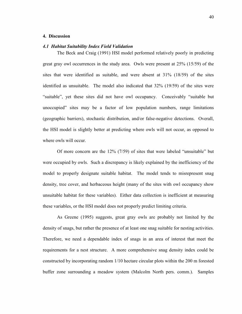
The Beck and Craig (1991) HSI model performed relatively poorly in predicting
great gray owl occurrences in the study area. Owls were present at 25% (15/59) of the
sites that were identified as suitable, and were absent at 31% (18/59) of the sites
identified as unsuitable. The model also indicated that 32% (19/59) of the sites were
“suitable”, yet these sites did not have owl occupancy. Conceivably “suitable but
unoccupied” sites may be a factor of low population numbers, range limitations
(geographic barriers), stochastic distribution, and/or false-negative detections. Overall,
the HSI model is slightly better at predicting where owls will not occur, as opposed to
where owls will occur.
Of more concern are the 12% (7/59) of sites that were labeled “unsuitable” but
were occupied by owls. Such a discrepancy is likely explained by the inefficiency of the
model to properly designate suitable habitat. The model tends to misrepresent snag
density, tree cover, and herbaceous height (many of the sites with owl occupancy show
unsuitable habitat for these variables). Either data collection is inefficient at measuring
these variables, or the HSI model does not properly predict limiting criteria.
As Greene (1995) suggests, great gray owls are probably not limited by the
density of snags, but rather the presence of at least one snag suitable for nesting activities.
Therefore, we need a dependable index of snags in an area of interest that meet the
requirements for a nest structure. A more comprehensive snag density index could be
constructed by incorporating random 1/10 hectare circular plots within the 200 m forested
buffer zone surrounding a meadow system (Malcolm North pers. comm.). Samples
41
would be stratified among different forest types (e.g. disturbed, undisturbed, late-seral,
mid-seral, etc.), with five plots per type.
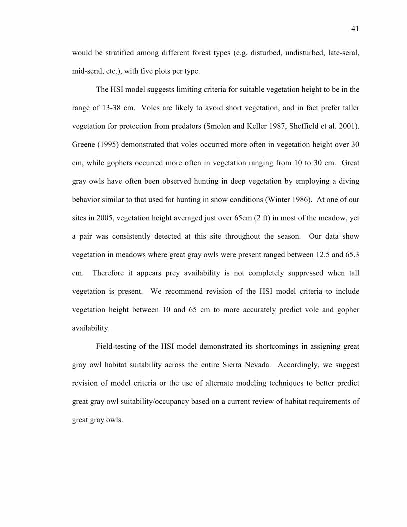
The HSI model suggests limiting criteria for suitable vegetation height to be in the
range of 13-38 cm. Voles are likely to avoid short vegetation, and in fact prefer taller
vegetation for protection from predators (Smolen and Keller 1987, Sheffield et al. 2001).
Greene (1995) demonstrated that voles occurred more often in vegetation height over 30
cm, while gophers occurred more often in vegetation ranging from 10 to 30 cm. Great
gray owls have often been observed hunting in deep vegetation by employing a diving
behavior similar to that used for hunting in snow conditions (Winter 1986). At one of our
sites in 2005, vegetation height averaged just over 65cm (2 ft) in most of the meadow, yet
a pair was consistently detected at this site throughout the season. Our data show
vegetation in meadows where great gray owls were present ranged between 12.5 and 65.3
cm. Therefore it appears prey availability is not completely suppressed when tall
vegetation is present. We recommend revision of the HSI model criteria to include
vegetation height between 10 and 65 cm to more accurately predict vole and gopher
availability.
Field-testing of the HSI model demonstrated its shortcomings in assigning great
gray owl habitat suitability across the entire Sierra Nevada. Accordingly, we suggest
revision of model criteria or the use of alternate modeling techniques to better predict
great gray owl suitability/occupancy based on a current review of habitat requirements of
great gray owls.
42
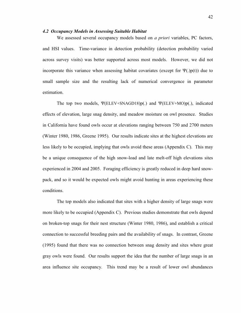
4.2 Occupancy Models in Assessing Suitable Habitat
We assessed several occupancy models based on a priori variables, PC factors,
and HSI values. Time-variance in detection probability (detection probability varied
across survey visits) was better supported across most models. However, we did not
incorporate this variance when assessing habitat covariates (except for Ψ(.)p(t)) due to
small sample size and the resulting lack of numerical convergence in parameter
estimation.
The top two models, Ψ(ELEV+SNAGD18)p(.) and Ψ(ELEV+MO)p(.), indicated
effects of elevation, large snag density, and meadow moisture on owl presence. Studies
in California have found owls occur at elevations ranging between 750 and 2700 meters
(Winter 1980, 1986, Greene 1995). Our results indicate sites at the highest elevations are
less likely to be occupied, implying that owls avoid these areas (Appendix C). This may
be a unique consequence of the high snow-load and late melt-off high elevations sites
experienced in 2004 and 2005. Foraging efficiency is greatly reduced in deep hard snow-
pack, and so it would be expected owls might avoid hunting in areas experiencing these
conditions.
The top models also indicated that sites with a higher density of large snags were
more likely to be occupied (Appendix C). Previous studies demonstrate that owls depend
on broken-top snags for their nest structure (Winter 1980, 1986), and establish a critical
connection to successful breeding pairs and the availability of snags. In contrast, Greene
(1995) found that there was no connection between snag density and sites where great
gray owls were found. Our results support the idea that the number of large snags in an
area influence site occupancy. This trend may be a result of lower owl abundances
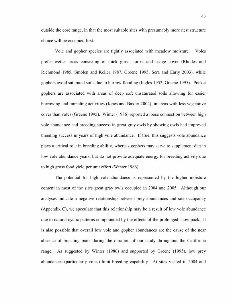
43
outside the core range, in that the most suitable sites with presumably more nest structure
choice will be occupied first.
Vole and gopher species are tightly associated with meadow moisture. Voles
prefer wetter areas consisting of thick grass, forbs, and sedge cover (Rhodes and
Richmond 1985, Smolen and Keller 1987, Greene 1995, Sera and Early 2003), while
gophers avoid saturated soils due to burrow flooding (Ingles 1952, Greene 1995). Pocket
gophers are associated with areas of deep soft unsaturated soils allowing for easier
burrowing and tunneling activities (Jones and Baxter 2004), in areas with less vegetative
cover than voles (Greene 1995). Winter (1986) reported a loose connection between high
vole abundance and breeding success in great gray owls by showing owls had improved
breeding success in years of high vole abundance. If true, this suggests vole abundance
plays a critical role in breeding ability, whereas gophers may serve to supplement diet in
low vole abundance years, but do not provide adequate energy for breeding activity due
to high gross food yield per unit effort (Winter 1986).
The potential for high vole abundance is represented by the higher moisture
content in most of the sites great gray owls occupied in 2004 and 2005. Although our
analyses indicate a negative relationship between prey abundances and site occupancy
(Appendix C), we speculate that this relationship may be a result of low vole abundance
due to natural cyclic patterns compounded by the effects of the prolonged snow pack. It
is also possible that overall low vole and gopher abundances are the cause of the near
absence of breeding pairs during the duration of our study throughout the California
range. As suggested by Winter (1986) and supported by Greene (1995), low prey
abundances (particularly voles) limit breeding capability. At sites visited in 2004 and

44
2005, prey abundances may have sustained daily activity of individual owls but did not
allow for breeding to occur. In addition, the low prey abundance may have facilitated
more of a migratory response in the foraging behavior of the great gray owl population.
Some habitat features, such as meadow moisture, herbaceous height, and
herbaceous cover, are variable over the course of the year. For example, moisture is at its
highest and vegetation height at its lowest during May and June due to recent snow cover
and continuous source of water from melting snow packs. Likewise, later months (e.g.
the Fall months of August and September) experience dry meadow and vegetation
conditions which directly relate to prey availability. Therefore depending on the time of
the season certain parameters will vary across time at a site. For this reason time constant
variables, such as elevation and snag density, may provide more robust predictors of site
occupancy.
When contrasting occupancy models incorporating PC factors and HSI values as
covariates with models incorporating a priori variables, models did not adequately
compare. The PCA analysis produced six factors, of which five largely overlapped a
priori variables. All six factors accounted for 75.1% of the variation in the data,
however, models that were developed containing these factors held almost no weight
compared to the top individual variable models. PCA can be valuable to reduce the
number of variables one considers in the modeling process, yet such an approach was not
useful in our study. Selecting variables that were believed to be useful predictors based
on current knowledge of great gray owl habitat requirements, proved to be more effective
in our study.
45
To provide a larger base of comparison between analytical approaches, we built
several models based on HSI variables and overall value. We found individual HS
variables representing herbaceous height, herbaceous cover, and snag presence had better
strength than the overall HSI value, however, when compared to top a priori models,
HSI models also show almost no weight. Contrasts between PC, HSI, and a priori
models suggest that selecting individual a priori covariates was better method to assess
of key habitat components related to great gray owl presence.
4.3 Occupancy Models in Estimating Ψ
For models incorporating a priori variables, the weighted model average for site
occupancy (Ψ) was 0.301, indicating that approximately 30% of sites with suitable
habitat were occupied by great gray owls across the study area. This was only marginally
better than the naïve estimate of 0.289, indicating the naïve estimate slightly under-
represents the actual proportion of site occupied across the study area. According to
MacKenzie et al. (2002), estimates of Ψ tend to be positively biased with small number
visits per site, which may be the case in our study with an average of 4.6 visits per site
per year. Regardless, the low proportion of sites occupied suggests that suitable habitat is
not being filled by great gray owls. We believe this is mainly due to low population
numbers, however site availability may add to the issue. Site availability may be affected
by barriers to dispersal (i.e. site connectivity) such as isolation of suitable sites by large
distances or impassable geography, however, these questions were not addressed within
the scope of this study.
46
4.4 Implications of Study
It is important to note that inclusion of sites within the core range represents a
fundamental difference in the sampling scheme throughout the regional scope of the
project. Site selection inside the core range was not uniquely based off of GIS mapping
as were areas outside of the core. Undoubtedly this could lead to parameter estimation
bias and surveyor bias (i.e. surveyors may anticipate owl detections at historic sites or
know specific locations of historic detections thus positively biasing survey results).
However, we felt justified in using a pooled dataset containing sites both inside and
outside the core range due to similar distributions of key habitat variables for all sites
visited in 2004 and 2005 (Appendix C), and we believe overall results can prove useful in
assessing parameter estimations, survey effectiveness, and important habitat
characteristic differences inside and outside the core range.
In this study we have been successful in evaluating Beck and Craig’s (1991) HSI
model using sites located throughout the entire Sierra Nevada and at recommending
improvements to the model to better represent suitable habitat. We were able to assess
the application of several modeling techniques and found using a priori variables in the
occupancy model better supported the available data. We were also able to estimate
proportion of sites occupied by great gray owls throughout the Sierra, and to designate
important habitat components related to site occupancy.
We recognize the shortcomings of our study mainly due to small sample sizes and
differences in sampling scheme. Obtaining a large sample size is difficult when working
with a rare species outside its core range, but such an effort will be necessary for over the
long term to fully comprehend factors that relate to the sustainability of great gray owls.
A uniform sampling scheme for all sites would be recommended for future studies.
47
We consider this study as part of a working base for further study in California.
Areas in need of additional research include: (1) continued monitoring in potentially
suitable habitat across the entire Sierra Nevada to further understand great gray owl
distribution; (2) banding and radio tracking to understand winter/summer foraging habits
and source/sink dynamics; (3) concentrated habitat sampling of sites to understand
possible habitat preference differences and similarities inside and outside of the core
range; (4) development of dependable indices to assess important habitat components
such as food availability and snag density; (5) small mammal trapping to understand how
prey abundance relates to occupancy and breeding success; (6) genetic sampling of
individuals across the range to assess differences/similarities of genetic relatedness
between the isolated populations in California to other populations within the continent,
and (7) revision of survey protocol.

48
Figures and Tables
Figure 1. Map of California indicating 2004 and 2005 habitat assessment sites.

49
Figure 2. Diagram of habitat sampling scheme showing meadow and forest transects.
Image adopted from Greene (1995).
200 meters
forest transect
= prey data point
= veg data point
meadow forest
meadow transect
in 2005
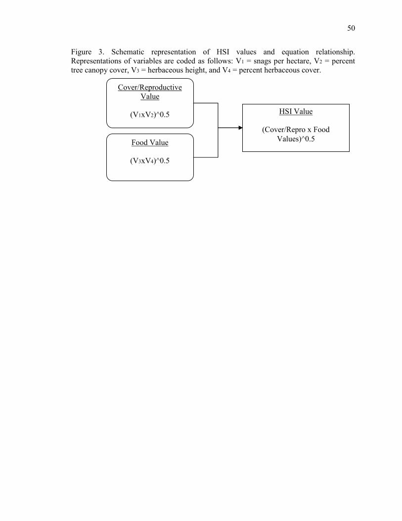
50
Figure 3. Schematic representation of HSI values and equation relationship.
Representations of variables are coded as follows: V1 = snags per hectare, V2 = percent
tree canopy cover, V3 = herbaceous height, and V4 = percent herbaceous cover.
Cover/Reproductive
Value
(V1xV2)^0.5
Food Value
(V3xV4)^0.5
HSI Value
(Cover/Repro x Food
Values)^0.5
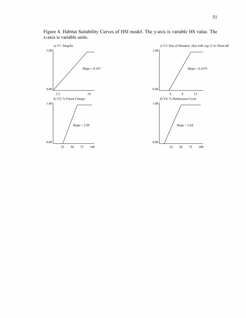
51
Figure 4. Habitat Suitability Curves of HSI model. The y-axis is variable HS value. The
x-axis is variable units.
1.00
0.00
a) V1: Snag/ha
b) V2: % Forest Canopy
1.00
0.00
1.00
0.00
1.00
0.00
c) V3: Size of Meadow (ha) with veg 13 to 38cm tall
d) V4: % Herbaceous Cover
2.5 10
Slope = 0.107
25 50 75 100 25 50 75 100
4 8 12
Slope = 2.64 Slope = 2.50
Slope = 0.1675
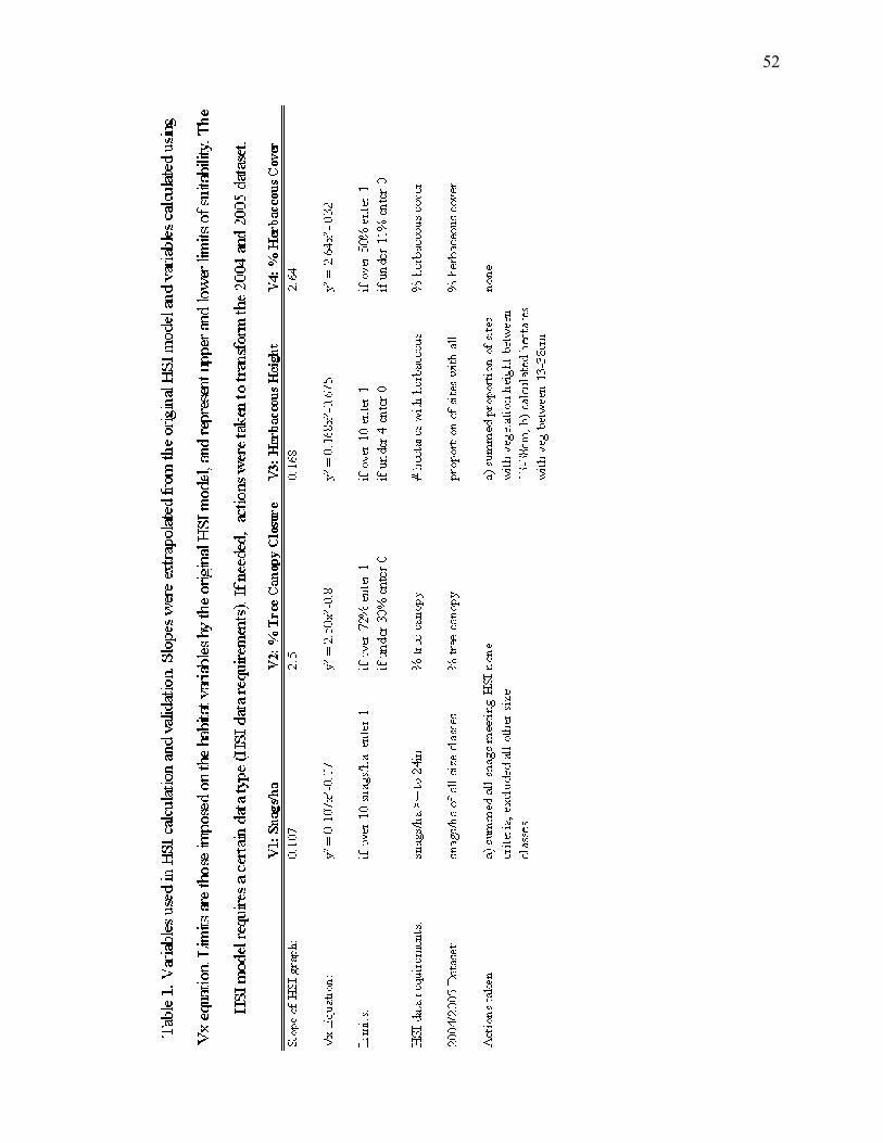
52

53
Table 2. Abbreviations and definitions for continuous and categorical habitat variables
collected at 52 sites across the Sierra Nevada in 2004 and 2005.
Abreviation: Definition:
ELEV Elevation of site (feet)
ACRES Size of meadow (acres)
HCOV % herbaceous cover in meadow
PTGRASS % grass in meadow
PTFORB % forbs in meadow
PTRUSH % rush in meadow
PTSEDGE % sedge in meadow
HGHT Average herbaceous height in meadow (cm)
PTDRY % dry soil in meadow
PTMOIST % moist soil in meadow
PTSAT % saturated soil in meadow
PTSTW % standing water in meadow
MO Moisture index in meadow (1 to 4 = dry to standing water)
GO Gopher abundance index in meadow
VO Vole abundance index in meadow
GOVO Combined gopher and vole abundance index in meadow
FCOV % forest canopy cover
SNAGD Total snag density index (snags/hectare)
SNAGD18 Snag >= 18in dbh density index (snags/hectare)
PTFIR % fir species in 200m forested buffer surrounding meadow
GRAZ (categorical variable) Current grazing activity (1=grazed, 2=not grazed)
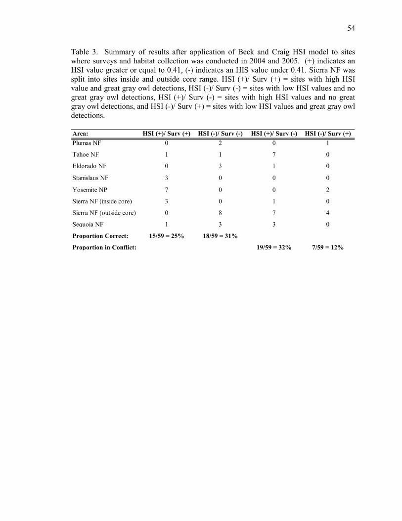
54
Table 3. Summary of results after application of Beck and Craig HSI model to sites
where surveys and habitat collection was conducted in 2004 and 2005. (+) indicates an
HSI value greater or equal to 0.41, (-) indicates an HIS value under 0.41. Sierra NF was
split into sites inside and outside core range. HSI (+)/ Surv (+) = sites with high HSI
value and great gray owl detections, HSI (-)/ Surv (-) = sites with low HSI values and no
great gray owl detections, HSI (+)/ Surv (-) = sites with high HSI values and no great
gray owl detections, and HSI (-)/ Surv (+) = sites with low HSI values and great gray owl
detections.
Area: HSI (+)/ Surv (+) HSI (-)/ Surv (-) HSI (+)/ Surv (-) HSI (-)/ Surv (+)
Plumas NF 0 2 0 1
Tahoe NF 1 1 7 0
Eldorado NF 0 3 1 0
Stanislaus NF 3 0 0 0
Yosemite NP 7 0 0 2
Sierra NF (inside core) 3 0 1 0
Sierra NF (outside core) 0 8 7 4
Sequoia NF 1 3 3 0
Proportion Correct: 15/59 = 25% 18/59 = 31%
Proportion in Conflict: 19/59 = 32% 7/59 = 12%
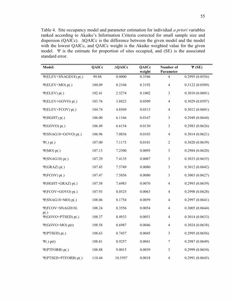
55
Table 4. Site occupancy model and parameter estimation for individual a priori variables
ranked according to Akaike’s Information Criteria corrected for small sample size and
dispersion (QAICc). ∆QAICc is the difference between the given model and the model
with the lowest QAICc, and QAICc weight is the Akaike weighted value for the given
model. Ψ is the estimate for proportion of sites occupied, and (SE) is the associated
standard error.
Model: QAICc ∆QAICc QAICc
weight
Number of
Parameter
Ψ (SE)
Ψ(ELEV+SNAGD18) p(.) 99.88 0.0000 0.3546 4 0.2995 (0.0556)
Ψ(ELEV+MO) p(.) 100.09 0.2104 0.3192 4 0.3122 (0.0589)
Ψ(ELEV) p(.) 102.41 2.5274 0.1002 3 0.3010 (0.0601)
Ψ(ELEV+GOVO) p(.) 103.76 3.8823 0.0509 4 0.3029 (0.0597)
Ψ(ELEV+FCOV) p(.) 104.74 4.8569 0.0313 4 0.3012 (0.0601)
Ψ(HGHT) p(.) 106.00 6.1166 0.0167 3 0.2949 (0.0644)
Ψ(GOVO) p(.) 106.49 6.6154 0.0130 3 0.2983 (0.0626)
Ψ(SNAG18+GOVO) p(.) 106.96 7.0836 0.0103 4 0.3014 (0.0621)
Ψ(.) p(.) 107.00 7.1173 0.0101 2 0.3020 (0.0639)
Ψ(MO) p(.) 107.13 7.2500 0.0095 3 0.2984 (0.0620)
Ψ(SNAG18) p(.) 107.29 7.4135 0.0087 3 0.3033 (0.0635)
Ψ(GRAZ) p(.) 107.45 7.5749 0.0080 3 0.3012 (0.0642)
Ψ(FCOV) p(.) 107.47 7.5856 0.0080 3 0.3003 (0.0627)
Ψ(HGHT+GRAZ) p(.) 107.58 7.6983 0.0076 4 0.2993 (0.0639)
Ψ(FCOV+GOVO) p(.) 107.93 8.0525 0.0063 4 0.2998 (0.0628)
Ψ(SNAG18+MO) p(.) 108.06 8.1754 0.0059 4 0.2997 (0.0641)
Ψ(FCOV+SNAGD18)
p(.)
108.24 8.3556 0.0054 4 0.3005 (0.0644)
Ψ(GOVO+PTSED) p(.) 108.37 8.4933 0.0051 4 0.3014 (0.0633)
Ψ(GOVO+MO) p(t) 108.58 8.6987 0.0046 4 0.3024 (0.0638)
Ψ(PTSED) p(.) 108.63 8.7457 0.0045 3 0.2995 (0.0656)
Ψ(.) p(t) 108.81 8.9257 0.0041 7 0.2987 (0.0649)
Ψ(PTFORB) p(.) 108.88 9.0015 0.0039 3 0.2999 (0.0654)
Ψ(PTSED+PTFORB) p(.) 110.44 10.5597 0.0018 4 0.2991 (0.0645)
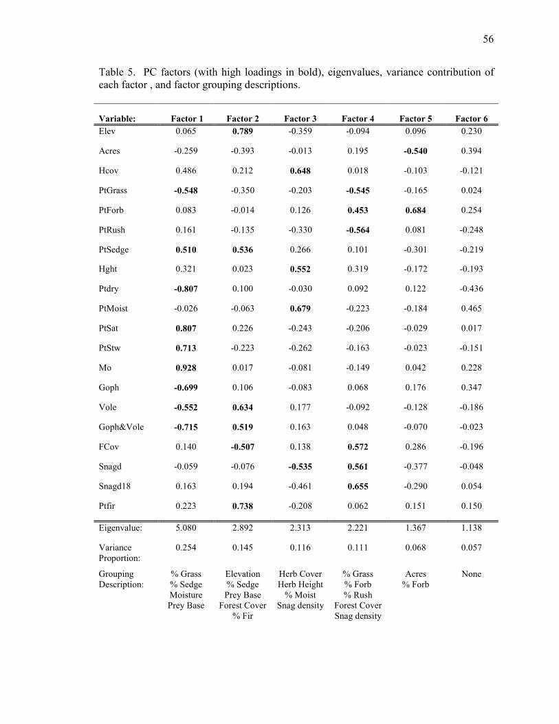
56
Table 5. PC factors (with high loadings in bold), eigenvalues, variance contribution of
each factor , and factor grouping descriptions.
Variable: Factor 1 Factor 2 Factor 3 Factor 4 Factor 5 Factor 6
Elev 0.065 0.789 -0.359 -0.094 0.096 0.230
Acres -0.259 -0.393 -0.013 0.195 -0.540 0.394
Hcov 0.486 0.212 0.648 0.018 -0.103 -0.121
PtGrass -0.548 -0.350 -0.203 -0.545 -0.165 0.024
PtForb 0.083 -0.014 0.126 0.453 0.684 0.254
PtRush 0.161 -0.135 -0.330 -0.564 0.081 -0.248
PtSedge 0.510 0.536 0.266 0.101 -0.301 -0.219
Hght 0.321 0.023 0.552 0.319 -0.172 -0.193
Ptdry -0.807 0.100 -0.030 0.092 0.122 -0.436
PtMoist -0.026 -0.063 0.679 -0.223 -0.184 0.465
PtSat 0.807 0.226 -0.243 -0.206 -0.029 0.017
PtStw 0.713 -0.223 -0.262 -0.163 -0.023 -0.151
Mo 0.928 0.017 -0.081 -0.149 0.042 0.228
Goph -0.699 0.106 -0.083 0.068 0.176 0.347
Vole -0.552 0.634 0.177 -0.092 -0.128 -0.186
Goph&Vole -0.715 0.519 0.163 0.048 -0.070 -0.023
FCov 0.140 -0.507 0.138 0.572 0.286 -0.196
Snagd -0.059 -0.076 -0.535 0.561 -0.377 -0.048
Snagd18 0.163 0.194 -0.461 0.655 -0.290 0.054
Ptfir 0.223 0.738 -0.208 0.062 0.151 0.150
Eigenvalue: 5.080 2.892 2.313 2.221 1.367 1.138
Variance
Proportion:
0.254 0.145 0.116 0.111 0.068 0.057
Grouping
Description:
% Grass
% Sedge
Moisture
Prey Base
Elevation
% Sedge
Prey Base
Forest Cover
% Fir
Herb Cover
Herb Height
% Moist
Snag density
% Grass
% Forb
% Rush
Forest Cover
Snag density
Acres
% Forb
None
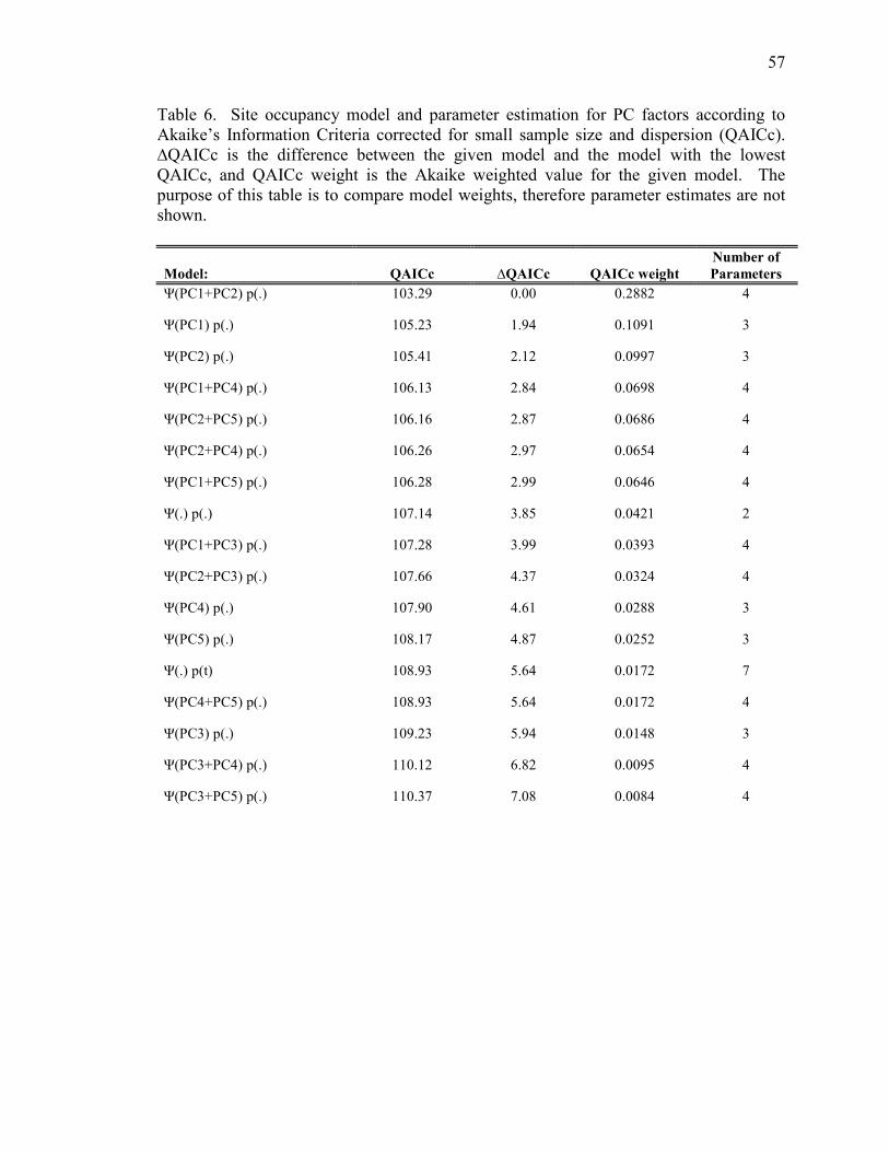
57
Table 6. Site occupancy model and parameter estimation for PC factors according to
Akaike’s Information Criteria corrected for small sample size and dispersion (QAICc).
∆QAICc is the difference between the given model and the model with the lowest
QAICc, and QAICc weight is the Akaike weighted value for the given model. The
purpose of this table is to compare model weights, therefore parameter estimates are not
shown.
Model: QAICc ∆QAICc QAICc weight
Number of
Parameters
Ψ(PC1+PC2) p(.) 103.29 0.00 0.2882 4
Ψ(PC1) p(.) 105.23 1.94 0.1091 3
Ψ(PC2) p(.) 105.41 2.12 0.0997 3
Ψ(PC1+PC4) p(.) 106.13 2.84 0.0698 4
Ψ(PC2+PC5) p(.) 106.16 2.87 0.0686 4
Ψ(PC2+PC4) p(.) 106.26 2.97 0.0654 4
Ψ(PC1+PC5) p(.) 106.28 2.99 0.0646 4
Ψ(.) p(.) 107.14 3.85 0.0421 2
Ψ(PC1+PC3) p(.) 107.28 3.99 0.0393 4
Ψ(PC2+PC3) p(.) 107.66 4.37 0.0324 4
Ψ(PC4) p(.) 107.90 4.61 0.0288 3
Ψ(PC5) p(.) 108.17 4.87 0.0252 3
Ψ(.) p(t) 108.93 5.64 0.0172 7
Ψ(PC4+PC5) p(.) 108.93 5.64 0.0172 4
Ψ(PC3) p(.) 109.23 5.94 0.0148 3
Ψ(PC3+PC4) p(.) 110.12 6.82 0.0095 4
Ψ(PC3+PC5) p(.) 110.37 7.08 0.0084 4
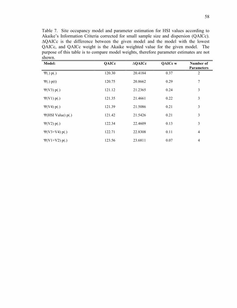
58
Table 7. Site occupancy model and parameter estimation for HSI values according to
Akaike’s Information Criteria corrected for small sample size and dispersion (QAICc).
∆QAICc is the difference between the given model and the model with the lowest
QAICc, and QAICc weight is the Akaike weighted value for the given model. The
purpose of this table is to compare model weights, therefore parameter estimates are not
shown.
Model: QAICc ∆QAICc QAICc w Number of
Parameters
Ψ(.) p(.) 120.30 20.4184 0.37 2
Ψ(.) p(t) 120.75 20.8662 0.29 7
Ψ(V3) p(.) 121.12 21.2365 0.24 3
Ψ(V1) p(.) 121.35 21.4661 0.22 3
Ψ(V4) p(.) 121.39 21.5086 0.21 3
Ψ(HSI Value) p(.) 121.42 21.5426 0.21 3
Ψ(V2) p(.) 122.34 22.4609 0.13 3
Ψ(V3+V4) p(.) 122.71 22.8308 0.11 4
Ψ(V1+V2) p(.) 123.56 23.6811 0.07 4
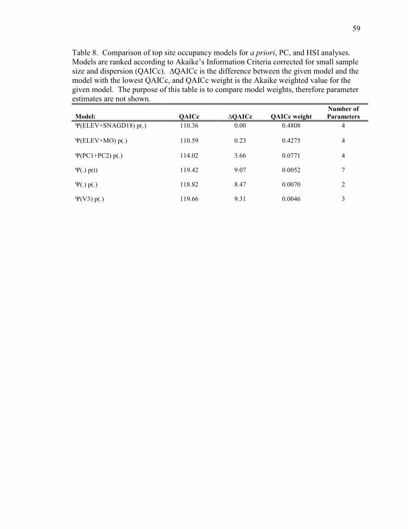
59
Table 8. Comparison of top site occupancy models for a priori, PC, and HSI analyses.
Models are ranked according to Akaike’s Information Criteria corrected for small sample
size and dispersion (QAICc). ∆QAICc is the difference between the given model and the
model with the lowest QAICc, and QAICc weight is the Akaike weighted value for the
given model. The purpose of this table is to compare model weights, therefore parameter
estimates are not shown.
Model: QAICc ∆QAICc QAICc weight
Number of
Parameters
Ψ(ELEV+SNAGD18) p(.) 110.36 0.00 0.4808 4
Ψ(ELEV+MO) p(.) 110.59 0.23 0.4275 4
Ψ(PC1+PC2) p(.) 114.02 3.66 0.0771 4
Ψ(.) p(t) 119.42 9.07 0.0052 7
Ψ(.) p(.) 118.82 8.47 0.0070 2
Ψ(V3) p(.) 119.66 9.31 0.0046 3
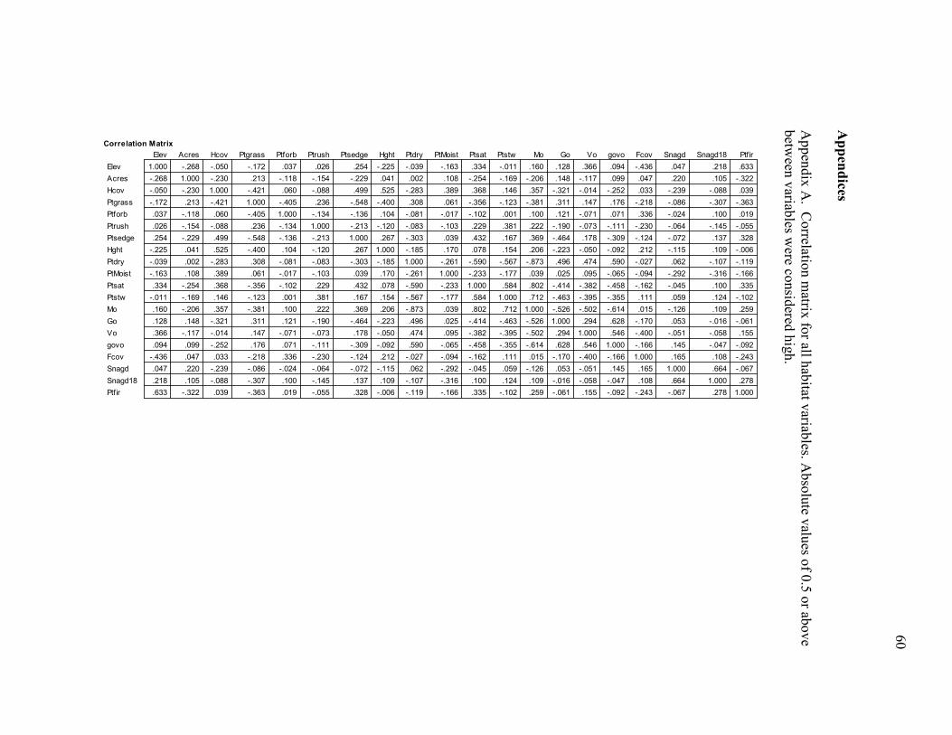
60
Appendices
Appendix A. C
orrelatio
n m
atrix fo
r all habitat v
ariables. A
bsolute v
alues o
f 0.5 or ab
ove
betw
een variab
les were co
nsid
ered high.
1.000 -.268 -.050 -.172 .037 .026 .254 -.225 -.039 -.163 .334 -.011 .160 .128 .366 .094 -.436 .047 .218 .633
-.268 1.000 -.230 .213 -.118 -.154 -.229 .041 .002 .108 -.254 -.169 -.206 .148 -.117 .099 .047 .220 .105 -.322
-.050 -.230 1.000 -.421 .060 -.088 .499 .525 -.283 .389 .368 .146 .357 -.321 -.014 -.252 .033 -.239 -.088 .039
-.172 .213 -.421 1.000 -.405 .236 -.548 -.400 .308 .061 -.356 -.123 -.381 .311 .147 .176 -.218 -.086 -.307 -.363
.037 -.118 .060 -.405 1.000 -.134 -.136 .104 -.081 -.017 -.102 .001 .100 .121 -.071 .071 .336 -.024 .100 .019
.026 -.154 -.088 .236 -.134 1.000 -.213 -.120 -.083 -.103 .229 .381 .222 -.190 -.073 -.111 -.230 -.064 -.145 -.055
.254 -.229 .499 -.548 -.136 -.213 1.000 .267 -.303 .039 .432 .167 .369 -.464 .178 -.309 -.124 -.072 .137 .328
-.225 .041 .525 -.400 .104 -.120 .267 1.000 -.185 .170 .078 .154 .206 -.223 -.050 -.092 .212 -.115 .109 -.006
-.039 .002 -.283 .308 -.081 -.083 -.303 -.185 1.000 -.261 -.590 -.567 -.873 .496 .474 .590 -.027 .062 -.107 -.119
-.163 .108 .389 .061 -.017 -.103 .039 .170 -.261 1.000 -.233 -.177 .039 .025 .095 -.065 -.094 -.292 -.316 -.166
.334 -.254 .368 -.356 -.102 .229 .432 .078 -.590 -.233 1.000 .584 .802 -.414 -.382 -.458 -.162 -.045 .100 .335
-.011 -.169 .146 -.123 .001 .381 .167 .154 -.567 -.177 .584 1.000 .712 -.463 -.395 -.355 .111 .059 .124 -.102
.160 -.206 .357 -.381 .100 .222 .369 .206 -.873 .039 .802 .712 1.000 -.526 -.502 -.614 .015 -.126 .109 .259
.128 .148 -.321 .311 .121 -.190 -.464 -.223 .496 .025 -.414 -.463 -.526 1.000 .294 .628 -.170 .053 -.016 -.061
.366 -.117 -.014 .147 -.071 -.073 .178 -.050 .474 .095 -.382 -.395 -.502 .294 1.000 .546 -.400 -.051 -.058 .155
.094 .099 -.252 .176 .071 -.111 -.309 -.092 .590 -.065 -.458 -.355 -.614 .628 .546 1.000 -.166 .145 -.047 -.092
-.436 .047 .033 -.218 .336 -.230 -.124 .212 -.027 -.094 -.162 .111 .015 -.170 -.400 -.166 1.000 .165 .108 -.243
.047 .220 -.239 -.086 -.024 -.064 -.072 -.115 .062 -.292 -.045 .059 -.126 .053 -.051 .145 .165 1.000 .664 -.067
.218 .105 -.088 -.307 .100 -.145 .137 .109 -.107 -.316 .100 .124 .109 -.016 -.058 -.047 .108 .664 1.000 .278
.633 -.322 .039 -.363 .019 -.055 .328 -.006 -.119 -.166 .335 -.102 .259 -.061 .155 -.092 -.243 -.067 .278 1.000
Elev Acres Hcov Ptgrass Ptforb Ptrush Ptsedge Hght Ptdry PtMoist Ptsat Ptstw Mo Go Vo govo Fcov Snagd Snagd18 Ptfir
Elev
Acres
Hcov
Ptgrass
Ptforb
Ptrush
Ptsedge
Hght
Ptdry
PtMoist
Ptsat
Ptstw
Mo
Go
Vo
govo
Fcov
Snagd
Snagd18
Ptfir
Correlation Matrix
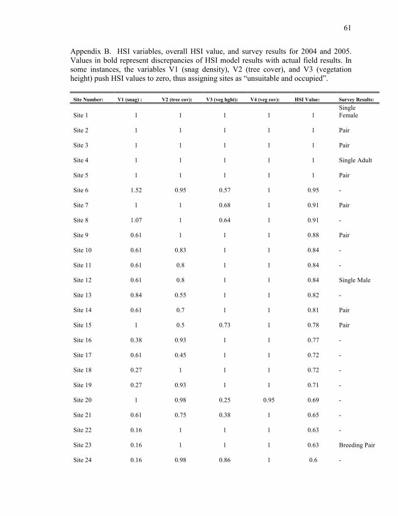
61
Appendix B. HSI variables, overall HSI value, and survey results for 2004 and 2005.
Values in bold represent discrepancies of HSI model results with actual field results. In
some instances, the variables V1 (snag density), V2 (tree cover), and V3 (vegetation
height) push HSI values to zero, thus assigning sites as “unsuitable and occupied”.
Site Number: V1 (snag) : V2 (tree cov): V3 (veg hght): V4 (veg cov): HSI Value: Survey Results:
Site 1 1 1 1 1 1
Single
Female
Site 2 1 1 1 1 1 Pair
Site 3 1 1 1 1 1 Pair
Site 4 1 1 1 1 1 Single Adult
Site 5 1 1 1 1 1 Pair
Site 6 1.52 0.95 0.57 1 0.95 -
Site 7 1 1 0.68 1 0.91 Pair
Site 8 1.07 1 0.64 1 0.91 -
Site 9 0.61 1 1 1 0.88 Pair
Site 10 0.61 0.83 1 1 0.84 -
Site 11 0.61 0.8 1 1 0.84 -
Site 12 0.61 0.8 1 1 0.84 Single Male
Site 13 0.84 0.55 1 1 0.82 -
Site 14 0.61 0.7 1 1 0.81 Pair
Site 15 1 0.5 0.73 1 0.78 Pair
Site 16 0.38 0.93 1 1 0.77 -
Site 17 0.61 0.45 1 1 0.72 -
Site 18 0.27 1 1 1 0.72 -
Site 19 0.27 0.93 1 1 0.71 -
Site 20 1 0.98 0.25 0.95 0.69 -
Site 21 0.61 0.75 0.38 1 0.65 -
Site 22 0.16 1 1 1 0.63 -
Site 23 0.16 1 1 1 0.63 Breeding Pair
Site 24 0.16 0.98 0.86 1 0.6 -
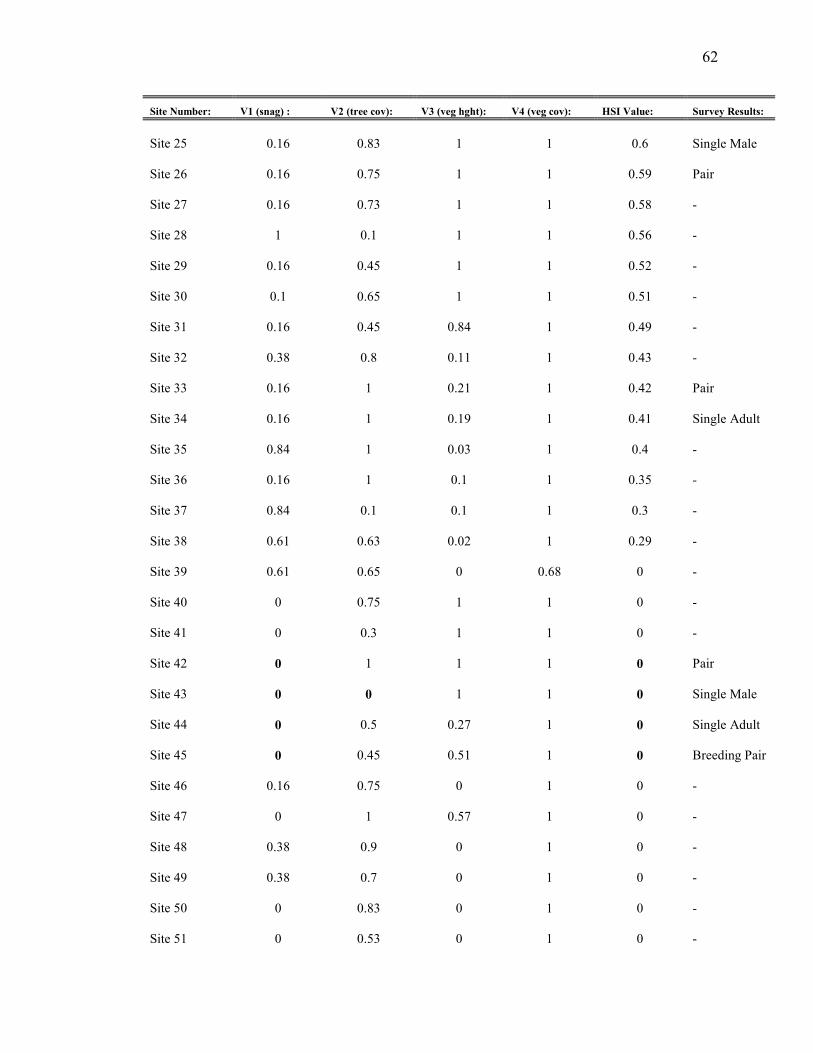
62
Site Number: V1 (snag) : V2 (tree cov): V3 (veg hght): V4 (veg cov): HSI Value: Survey Results:
Site 25 0.16 0.83 1 1 0.6 Single Male
Site 26 0.16 0.75 1 1 0.59 Pair
Site 27 0.16 0.73 1 1 0.58 -
Site 28 1 0.1 1 1 0.56 -
Site 29 0.16 0.45 1 1 0.52 -
Site 30 0.1 0.65 1 1 0.51 -
Site 31 0.16 0.45 0.84 1 0.49 -
Site 32 0.38 0.8 0.11 1 0.43 -
Site 33 0.16 1 0.21 1 0.42 Pair
Site 34 0.16 1 0.19 1 0.41 Single Adult
Site 35 0.84 1 0.03 1 0.4 -
Site 36 0.16 1 0.1 1 0.35 -
Site 37 0.84 0.1 0.1 1 0.3 -
Site 38 0.61 0.63 0.02 1 0.29 -
Site 39 0.61 0.65 0 0.68 0 -
Site 40 0 0.75 1 1 0 -
Site 41 0 0.3 1 1 0 -
Site 42 0 1 1 1 0 Pair
Site 43 0 0 1 1 0 Single Male
Site 44 0 0.5 0.27 1 0 Single Adult
Site 45 0 0.45 0.51 1 0 Breeding Pair
Site 46 0.16 0.75 0 1 0 -
Site 47 0 1 0.57 1 0 -
Site 48 0.38 0.9 0 1 0 -
Site 49 0.38 0.7 0 1 0 -
Site 50 0 0.83 0 1 0 -
Site 51 0 0.53 0 1 0 -
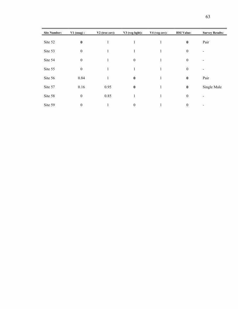
63
Site Number: V1 (snag) : V2 (tree cov): V3 (veg hght): V4 (veg cov): HSI Value: Survey Results:
Site 52 0 1 1 1 0 Pair
Site 53 0 1 1 1 0 -
Site 54 0 1 0 1 0 -
Site 55 0 1 1 1 0 -
Site 56 0.84 1 0 1 0 Pair
Site 57 0.16 0.95 0 1 0 Single Male
Site 58 0 0.85 1 1 0 -
Site 59 0 1 0 1 0 -

64
Appendix C. Stacked dot plots of 8 a priori variables showing relationships between
presence (1) and absence (0) in sites inside (closed dots) and outside (open dots) the core
range: a) elevation (ft), b) percent forbs, c) percent sedge, d) meadow vegetation height
(cm), c) moisture index, e) gopher and vole abundance, f) percent forest canopy cover,
and g) snag density >18in DBH per hectare.
a) elevation (ft)
Sit
e S
tatu
s
Elevation (ft)
7500
4500
4000
3500
7000
6500
6000
5500
5000
3000
0
1
b) percent forbs
Percent Forbs
1.00
0.30
0.20
0.10
0.80
0.70
0.60
0.50
0.40
0.00
0
1
Sit
e S
tatu
s
0.90
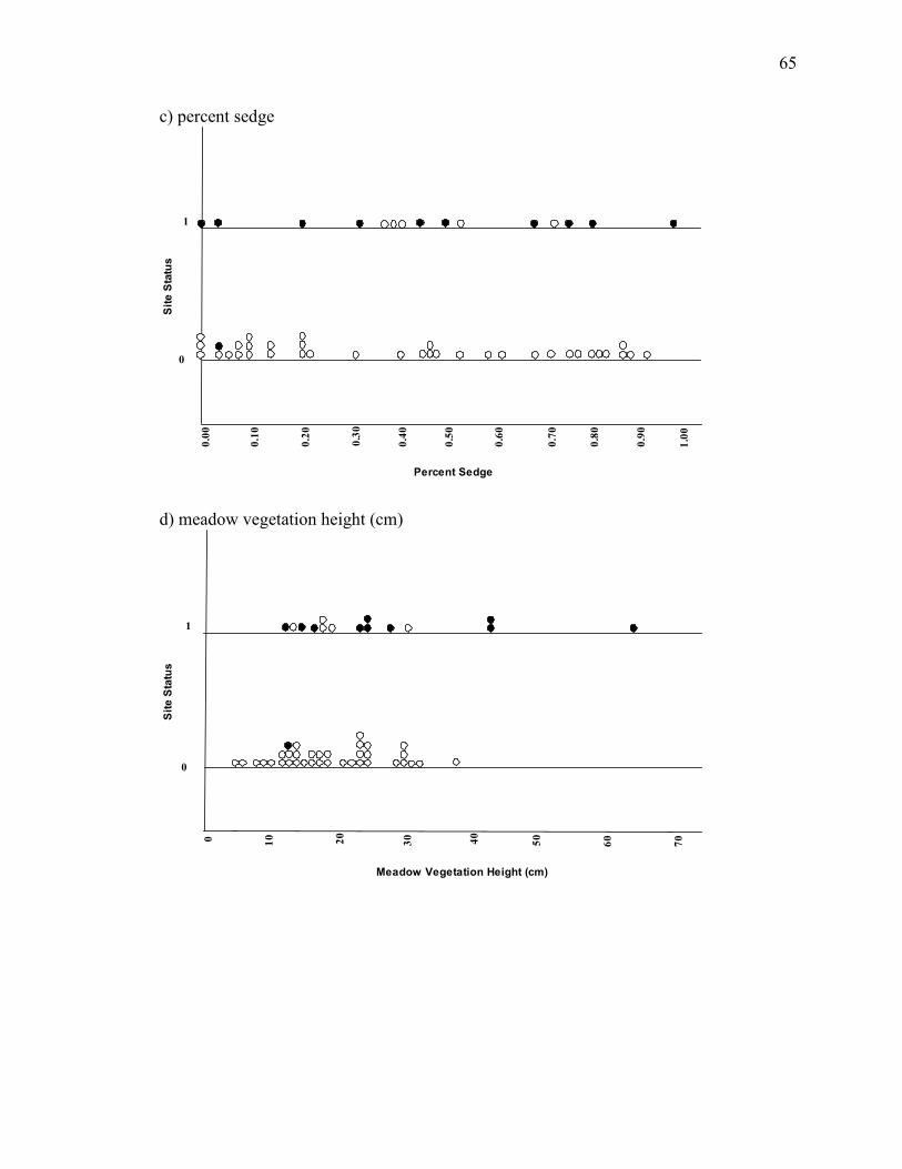
65
c) percent sedge
Sit
e S
tatu
s
Percent Sedge
1.00
0.30
0.20
0.10
0.80
0.70
0.60
0.50
0.40
0.00
0
1
0.90
d) meadow vegetation height (cm)
Meadow Vegetation Height (cm)
70
3020
10
60
50400
0
1
Sit
e S
tatu
s
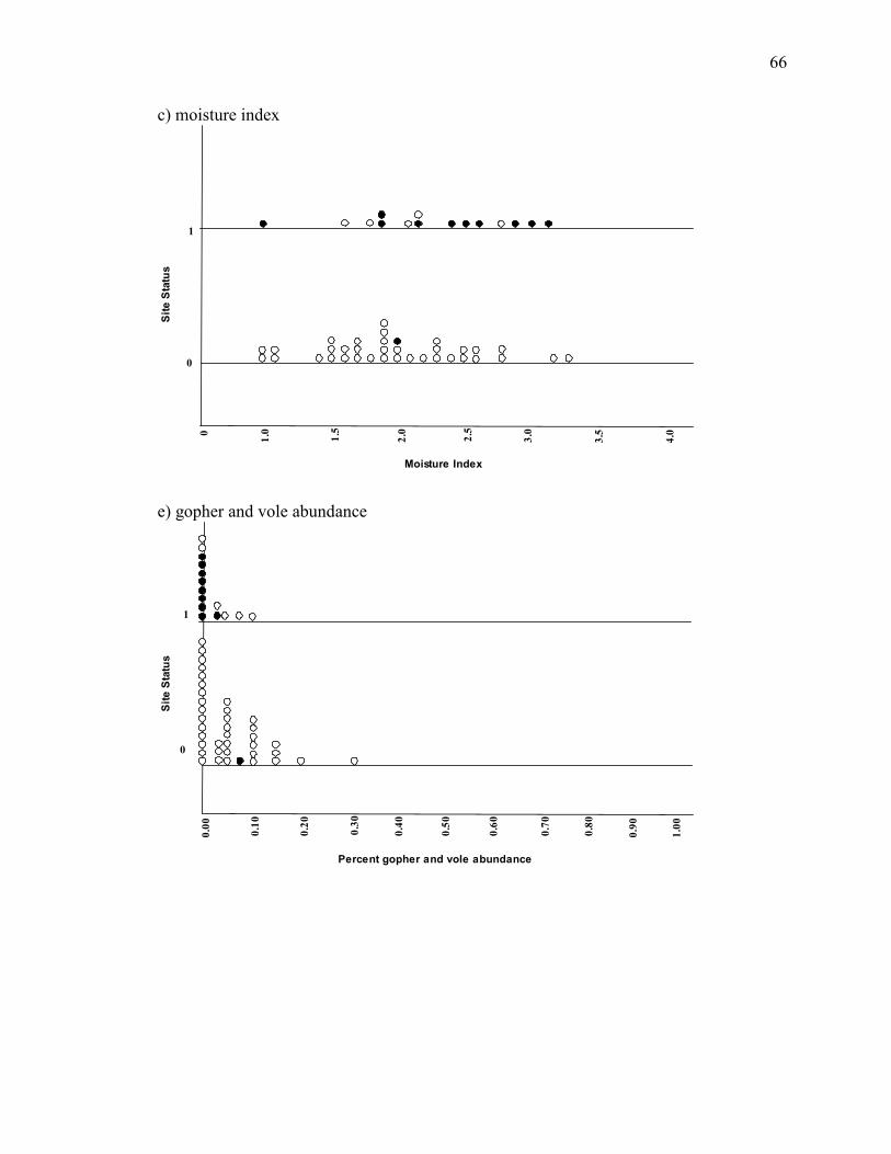
66
c) moisture index
Moisture Index
4.0
2.0
1.5
1.0
3.5
3.0
2.50
0
1
Sit
e S
tatu
s
e) gopher and vole abundance
Percent gopher and vole abundance
1.00
0.30
0.20
0.10
0.80
0.70
0.60
0.50
0.40
0.00
0
1
Sit
e S
tatu
s
0.90
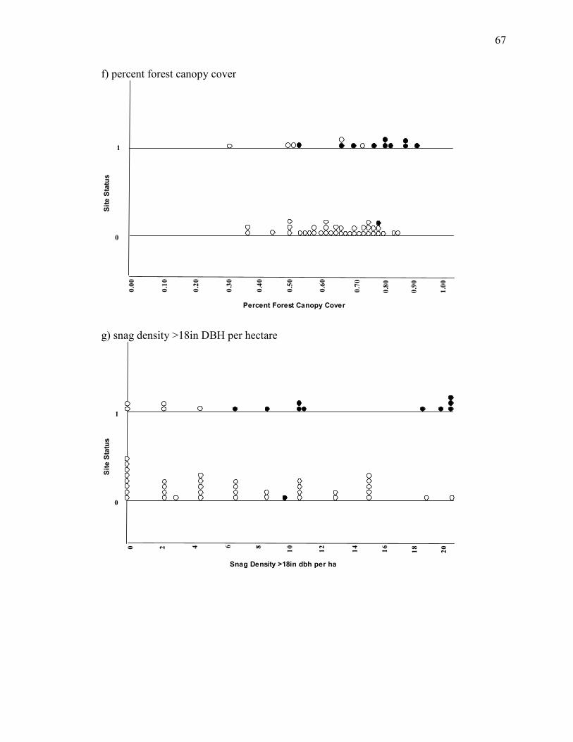
67
f) percent forest canopy cover
Percent Forest Canopy Cover
1.00
0.30
0.20
0.10
0.80
0.70
0.60
0.50
0.40
0.00
0
1
Sit
e S
tatu
s
0.90
g) snag density >18in DBH per hectare
Snag Density >18in dbh per ha
642
16
14
12
1080
0
1
Sit
e S
tatu
s
18
20
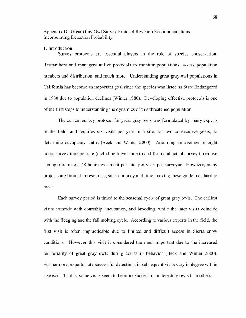
68
Appendix D. Great Gray Owl Survey Protocol Revision Recommendations
Incorporating Detection Probability.
1. Introduction
Survey protocols are essential players in the role of species conservation.
Researchers and managers utilize protocols to monitor populations, assess population
numbers and distribution, and much more. Understanding great gray owl populations in
California has become an important goal since the species was listed as State Endangered
in 1980 due to population declines (Winter 1980). Developing effective protocols is one
of the first steps to understanding the dynamics of this threatened population.
The current survey protocol for great gray owls was formulated by many experts
in the field, and requires six visits per year to a site, for two consecutive years, to
determine occupancy status (Beck and Winter 2000). Assuming an average of eight
hours survey time per site (including travel time to and from and actual survey time), we
can approximate a 48 hour investment per site, per year, per surveyor. However, many
projects are limited in resources, such a money and time, making these guidelines hard to
meet.
Each survey period is timed to the seasonal cycle of great gray owls. The earliest
visits coincide with courtship, incubation, and brooding, while the later visits coincide
with the fledging and the fall molting cycle. According to various experts in the field, the
first visit is often impracticable due to limited and difficult access in Sierra snow
conditions. However this visit is considered the most important due to the increased
territoriality of great gray owls during courtship behavior (Beck and Winter 2000).
Furthermore, experts note successful detections in subsequent visits vary in degree within
a season. That is, some visits seem to be more successful at detecting owls than others.
69
Assuming these statements are accurate, survey protocol should be examined to
assess success at detecting owls and feasibility of performing surveys. An effective
protocol not only saves valuable resources, but will allow wildlife managers and
conservation biologists to more successfully monitor the Sierra population of great gray
owls, and ultimately protect them from further decline.
McArdle (1990) developed a method to determine the number of visits required at
a site by incorporating error estimates into the assumption of a species’ absence with a
specified confidence. That is, the study developed a method to address questions relating
to the number of surveys needed with negative results to be confident a species is actually
absent from a site and not merely overlooked. For example, if we want a 95% confidence
level to determine if a site is unoccupied, we set ά = 0.05 and use the equation:
Nmin = log ά / log (1-p) (1)
Where p is the estimated detection probability, and Nmin is the resulting minimum
number of visits to attain the specified confidence level.
Kery (2002) applies this method on several snake species that have low detection
rates. However the study goes one step further by using a generalized linear mixed
model able to assess the relationship between detection probability and variables such as
habitat type, size of site, population size, and time of visit.
Our main objective in this study is to examine overall survey protocol for
effectiveness and variability in survey visit detection rates. To achieve this goal we will:
(1) use simple occupancy models to obtain an estimate on the detection probability (p);
and (2) determine the number of visits required to a site to establish occupancy status.
Original objectives incorporated survey specific covariates, such as temperature and

70
survey initiation time, to evaluate detection probability estimates and variables affecting
survey visit success. However, due to an absence of temperature and initiation time data
for all sites included in the dataset, we were unable to evaluate variables that may affect
detection probability at this time.
2. Methods
2.1 Study Area
We collected survey and habitat data in the Sierra Nevada mountain range in
California in areas across its entire expanse, including sites in Plumas, Tahoe, Eldorado,
Sierra, and Sequoia National Forests, and Yosemite National Park. All sites were
surveyed by CDFG crews with the exception of those within Yosemite National Park.
Yosemite sites were surveyed by a NPS biologist and Forest Service crew in 2005. All
surveys followed the same protocol and are therefore comparable in nature.
2.2 Survey Protocol
We adopted survey guidelines primarily from the more extensive USDA Forest
Service protocol (Beck and Winter 2000). Walking and driving transects were used for
surveys depending on road access and meadow structure. Walking routes were placed
along meadow borders, just inside the forest canopy. Driving routes were placed within
200 m of the meadow’s edge. All survey points were spaced 0.15 to 0.20 miles apart. A
calling device was used to generate broadcast calls played at each survey point. The
calling sequence at each survey station lasted eight minutes followed by 2 minutes of
quiet listening time.

71
We conducted two to six visits at each site per year, generally in March to
September. According to Beck and Winter (2000) the most valuable visit is thought to be
during courtship, due to territoriality of the males. Therefore, we made concerted efforts
to conduct two to three nighttime visits during the early nesting season (courtship and
incubation periods), occurring from sunset to 1 or 2 am. In addition, one to two
nighttime visits took place within the late nesting season (brooding and post-fledge
periods), occurring 2 hours before sunset lasting through 2-4 hours past sunset. At most
sites we conducted a final visit during the day as a meadow search. During this time the
surveyor(s) searched for molted feathers, regurgitated pellets, whitewash on snags and
under roost sites, foraging perches within or near the meadow, and visual or auditory
detection of an owl. A positive identification was confirmed only by visual or audio
detection, or the presence of feathers.
2.3 Site Sampling
We utilized knowledge of great gray owl habitat preferences to produce a GIS-
based habitat suitability model, which was then used to select survey sites in the Sierra
Nevada of California outside the owl’s core range. Habitat preferences were derived
partially from the Habitat Suitability Index (HSI) model and management prescription for
the Great Gray Owl in California (Beck and Craig 1991), and partially on habitat
requirements known from the past research in California (Winter 1986, Greene 1995).
The HSI model was designed to predict habitat that is “comprised of mature or old-
growth conifer forests with dense canopy and numerous snags in close proximity to large
meadows or meadow systems” (Beck and Craig 1991). Based on a portion of the HSI
72
model criteria and known habitat preferences, we used variables for canopy closure
(USDA Forest Service Calveg 2000 Vegetation layer), meadow size (CDFG Sierra
Nevada Meadow Map layer), and Wildlife Habitat Relationship System (WHR) density
and size classification in GIS software to rank each meadow according to level of
suitability. We then selected sites representative of all status types for owls (i.e. known,
unknown, and historic), giving priority to sites with higher suitability ranks.
We surveyed both sites with historical use by great gray owls and sites where use
by great gray owls was unknown. In total, 60 sites were surveyed for owls and sampled
for habitat components in 2004 and 2005. Sixteen sites were sampled within the core
range, and 44 were sampled outside of that range (including known and unknown
occupancy status) (Figure 1). Eight of these sites were excluded from the dataset due to
lack of partial data or duplicate surveys over multiple years. Therefore the total number
of sites used in subsequent analyses was 52. The GIS-based model was not used to select
sites inside the core, but rather were selected based on historic owl presence to increase
sample size.
2.4 Data Analysis
Following MacKenzie et al. (2002), we used site occupancy modeling to estimate
detection probabilities. We ran two simple models using the 2004 and 2005 52-site
dataset for areas inside and outside the core range, where Ψ was constant over time and p
was either constant or variable over time (Ψ(.)p(.) and Ψ(.)p(t)).
The models were run using the program PRESENCE 2.0, and thereafter ranked
using Akaike’s Information Criterion (AIC) (Burnham and Anderson 2002). We
73
corrected AIC values for over or under dispersion (using c-hat; the quasi-likelihood
parameter) and small sample size according to Burnham and Anderson (2002), hereafter
referred to as QAICc.
To examine the number of visits required to ascertain great gray owl absence at a
site, the time-constant detection probability estimate was used in equation (1). We then
calculated the minimum number of visits to a site to affirm a site is not occupied during a
survey season with a 95% confidence level by setting ά = 0.05.
3. Results
In 2004 we attempted to make six visits per site, and in 2005 the goal was to make
at least four visits per site. Both years had an unusually high snow-load and late melt-off
date making access problematic, particularly so in 2005. Ultimately, limited access to
sites decreased the number of surveys conducted over both years. Sites received on
average 4.6 visits per year (2-6 visits/site/year) with a higher concentration of visits later
in the season.
Between the simple models, time dependence (Ψ(.)p(t); QAICc weight = 0.8547)
was better supported (Table A), and had a detection probability of 0.5862 (Table B).
Using this parameter in equation (1), Nmin equaled 3.40, indicating that one must make
at least 4 survey visits per site to affirm absence with a 95% confidence. The time
dependent detection probabilities for the model Ψ(.)p(t) were 0.7454, 1.000, 0.6014,
0.2264, 0.6546, and 0.7498 for visits 1 through 6 respectively (Table B).
4. Discussion
74
Survey protocol success is important to understanding owl distribution and
abundances. Management and conservation plans depend on protocols that use resources
sparingly while maintaining a level of effectiveness. The number of visits per site and
confidence in species detection are important considerations.
Our study showed varying degrees of detection probability among visits; the 1st,
2nd, and 6
th visits had higher detection probability, the 3
rd and 5
th had moderate detection
probability, and the 4th visit had the lowest detection probability. These visits correspond
to seasonal life cycles of breeding great gray owls (Table C). It is reasonable the first and
second visit (courtship/incubation) and last visit (post-molt) show high detection
probability. Male owls tend to be more territorial during the courtship period and readily
respond to playback calls (Beck and Winter 2000). The last visit consists of a daytime
search to look for signs of owl presence. If owls have been using the site regularly it is
relatively easy to find molted feathers in the vicinity.
Moderate detection probabilities were found for the post-fledge period (visit 5),
which denotes the time after which the young fledge from the nest but remain dependent
on the parents for food. Visit 5 is a highly vocal period for the young as begging for food
is regular. Broadcast calls played during this time include begging calls of the young and
female nest chatter. It is thought that playing these calls will readily instigate
vocalizations from the young, if in fact young are present. Young were only found at two
sites during 2004 and 2005 surveys, however, they did respond to the broadcast calls
through immediate and intense begging calls.
The brooding period (visit 4) shows a much lower detection probability. If
breeding, during this time the owls have settled into caring for the young. Females rarely
75
leave the nest at this point, and males are busy finding for the female, young, and himself
(Bull and Duncan 1993). It is possible during this period responses are further reduced
due to predator evasion, as the young and mother are more susceptible to attacks from
great horned owls, ravens, and various other raptors. The number of successful breeding
sites was low during the length of the study, therefore some other undetected factor must
have been acting to reduce detection probabilities during this period.
We would expect visit 3 (incubation) to also have a low detection probability
similar to visit 4, however this was not the case. If adults were tending an active nest, we
would expect a lower detection probability, especially from the nest area. However, the
seemingly low breeding activity and success would generate a higher detection rate than
expected under high breeding activity.
Current protocol calls for six visits per site per year to determine residency of
great gray owls. This equates to twelve visits, averaging 48 hours investment per site per
year (approximately 8 hours/visit counting survey time and travel time). Taking into
account the time-constant detection probability (0.5862), our results indicate number of
surveys can be reduced from 6 to 4 while maintaining a 95% confidence the species is
absent if recorded absent for all surveys. We recommend limiting surveys to include
visits 2, 3, 5, and 6. This would decrease resource investment by approximately 33%
while assuring a certain degree of confidence. If however early season access is granted,
visit 1 is preferable to visit 3.
By reducing number of surveys required we can reduce the number of hours spent
at a site, and ultimately reduce resource expenditures. In addition, by decreasing the
number of surveys to a site we can allocate more effort into increasing survey coverage

76
across the entire Sierra Nevada. This will allow information gaps, such as an
understanding of complete distribution and population numbers, to be bridged. And
lastly, the consequences of an effective survey protocol will aid efforts of wildlife
managers and conservation biologist to develop management plans that will sustain the
great gray owl population throughout the entire Sierra.
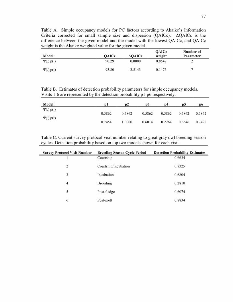
77
Table A. Simple occupancy models for PC factors according to Akaike’s Information
Criteria corrected for small sample size and dispersion (QAICc). ∆QAICc is the
difference between the given model and the model with the lowest QAICc, and QAICc
weight is the Akaike weighted value for the given model.
Model: QAICc ∆QAICc
QAICc
weight
Number of
Parameter
Ψ(.) p(.) 90.29 0.0000 0.8547 2
Ψ(.) p(t) 93.80 3.5143 0.1475 7
Table B. Estimates of detection probability parameters for simple occupancy models.
Visits 1-6 are represented by the detection probability p1-p6 respectively.
Model: p1 p2 p3 p4 p5 p6
Ψ(.) p(.) 0.5862 0.5862 0.5862 0.5862 0.5862 0.5862
Ψ(.) p(t) 0.7454 1.0000 0.6014 0.2264 0.6546 0.7498
Table C. Current survey protocol visit number relating to great gray owl breeding season
cycles. Detection probability based on top two models shown for each visit.
Survey Protocol Visit Number Breeding Season Cycle Period Detection Probability Estimates
1 Courtship 0.6634
2 Courtship/Incubation 0.8325
3 Incubation 0.6804
4 Brooding 0.2810
5 Post-fledge 0.6074
6 Post-molt 0.8834
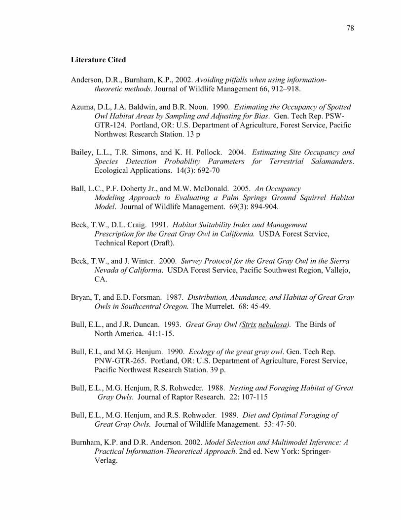
78
Literature Cited
Anderson, D.R., Burnham, K.P., 2002. Avoiding pitfalls when using information-
theoretic methods. Journal of Wildlife Management 66, 912–918.
Azuma, D.L, J.A. Baldwin, and B.R. Noon. 1990. Estimating the Occupancy of Spotted
Owl Habitat Areas by Sampling and Adjusting for Bias. Gen. Tech Rep. PSW-
GTR-124. Portland, OR: U.S. Department of Agriculture, Forest Service, Pacific
Northwest Research Station. 13 p
Bailey, L.L., T.R. Simons, and K. H. Pollock. 2004. Estimating Site Occupancy and
Species Detection Probability Parameters for Terrestrial Salamanders.
Ecological Applications. 14(3): 692-70
Ball, L.C., P.F. Doherty Jr., and M.W. McDonald. 2005. An Occupancy
Modeling Approach to Evaluating a Palm Springs Ground Squirrel Habitat
Model. Journal of Wildlife Management. 69(3): 894-904.
Beck, T.W., D.L. Craig. 1991. Habitat Suitability Index and Management
Prescription for the Great Gray Owl in California. USDA Forest Service,
Technical Report (Draft).
Beck, T.W., and J. Winter. 2000. Survey Protocol for the Great Gray Owl in the Sierra
Nevada of California. USDA Forest Service, Pacific Southwest Region, Vallejo,
CA.
Bryan, T, and E.D. Forsman. 1987. Distribution, Abundance, and Habitat of Great Gray
Owls in Southcentral Oregon. The Murrelet. 68: 45-49.
Bull, E.L., and J.R. Duncan. 1993. Great Gray Owl (Strix nebulosa). The Birds of
North America. 41:1-15.
Bull, E.L, and M.G. Henjum. 1990. Ecology of the great gray owl. Gen. Tech Rep.
PNW-GTR-265. Portland, OR: U.S. Department of Agriculture, Forest Service,
Pacific Northwest Research Station. 39 p.
Bull, E.L., M.G. Henjum, R.S. Rohweder. 1988. Nesting and Foraging Habitat of Great
Gray Owls. Journal of Raptor Research. 22: 107-115
Bull, E.L., M.G. Henjum, and R.S. Rohweder. 1989. Diet and Optimal Foraging of
Great Gray Owls. Journal of Wildlife Management. 53: 47-50.
Burnham, K.P. and D.R. Anderson. 2002. Model Selection and Multimodel Inference: A
Practical Information-Theoretical Approach. 2nd ed. New York: Springer-
Verlag.

79
California Native Plant Society Vegetation Committee. 2003. CNPS Releve Protocol.
Cooch, E., and G. White. 2005. Program MARK: A Gentle Introduction. 4th ed.
www.phidot.org/software/mark/docs/book
Defos du Rau, P., C. Barbraud, and J. Mondain-Monval. 2005. Incorporating
uncertainty into analysis of red-crested pochard habitat selection. Biological
Conservation. 125: 355-367.
Fetz, T.W., S.W. Janes, and H. Lauchstedt. 2003. Habitat Characteristics of Great Gray
Owl Sites in the Siskiyou Mountiansof Southwestern Oregon. The Journal of
Raptor Research. 37(4): 315-322.
Field, S.A., A.J. Tyre, K. H. Thorn, P.J. O'Connor, and H.P. Possingham. 2005.
Improving the efficiency of wildlife monitoring by estimating detectability: a case
study of foxes (Vulpes vulpes) on the Eyre Peninsula, South Australia. Wildlife
Research. 32: 253-258.
Finley, D.J., G.C. White, and J.P. Fitzgerald. 2005. Estimation of Swift Fox Population
Size and Occupancy Rates in Eastern Colorado. Journal of Wildlife Management.
69(3): 861-873
Greene, C. 1995. Habitat Requirements of Great Gray Owls in the Central Sierra
Nevada. M.S. Thesis. University of Michigan, MI.
Gu, W., and R.K. Swihart. 2004. Absent or undetected? Effects of non-detection of
species occurrence on wildlife-habitat models. Biological Conservation.
116:195-203.
Hayward, G.D. ed., and J. Verner ed. 1994. Flammulated, Boreal, and Great Gray Owls
in the United States: A Technical Conservation Assessment. USDA GTR-RM-
253.
Ingles, L.G. 1952. The ecology of the mountain pocket gopher, Thomomys monticola.
Ecology. 88: 87-95.
Jones, C.A., and C.N. Baxter. 2004. Thomomys bottae. Mammalian Species. 742: 1-14.
Krebs, C.J. 2003. Ecological Methodology. 2nd edition. Benjamin Cummings
Publishers, New York, 554p.
Kery, M. 2002. Inferring the absence of a species: a case study of snakes. Journal of
Wildlife Management. 66(2): 330-338.
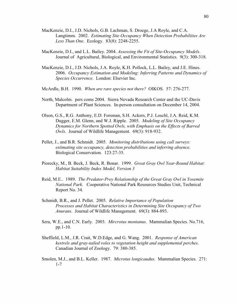
80
MacKenzie, D.I., J.D. Nichols, G.B. Lachman, S. Droege, J.A Royle, and C.A.
Langtimm. 2002. Estimating Site Occupancy When Detection Probabilities Are
Less Than One. Ecology. 83(8): 2248-2255.
MacKenzie, D.I., and L.L. Bailey. 2004. Assessing the Fit of Site-Occupancy Models.
Journal of Agricultural, Biological, and Environmental Statistics. 9(3): 300-318.
MacKenzie, D.I., J.D. Nichols, J.A. Royle, K.H. Pollock, L.L. Bailey, and J.E. Hines.
2006. Occupancy Estimation and Modeling: Inferring Patterns and Dynamics of
Species Occurrence. London: Elsevier Inc.
McArdle, B.H. 1990. When are rare species not there? OIKOS. 57: 276-277.
North, Malcolm. pers coms 2004. Sierra Nevada Research Center and the UC-Davis
Department of Plant Sciences. In-person consultation on December 14, 2004.
Olson, G.S., R.G. Anthony, E.D. Forsman, S.H. Ackers, P.J. Loschl, J.A. Reid, K.M.
Dugger, E.M. Glenn, and W.J. Ripple. 2005. Modeling of Site Occupancy
Dynamics for Northern Spotted Owls, with Emphasis on the Effects of Barred
Owls. Journal of Wildlife Management. 69(3): 918-932.
Pellet, J., and B.R. Schmidt. 2005. Monitoring distributions using call surveys:
estimating site occupancy, detection probabilities and inferring absence.
Biological Conservation. 123:27-35.
Piorecky, M., B. Beck, J. Beck, R. Bonar. 1999. Great Gray Owl Year-Round Habitat:
Habitat Suitability Index Model, Version 3
Reid, M.E.. 1989. The Predator-Prey Relationship of the Great Gray Owl in Yosemite
National Park. Cooperative National Park Resources Studies Unit, Technical
Report No. 34.
Schmidt, B.R., and J. Pellet. 2005. Relative Importance of Population
Processes and Habitat Characteristics in Determining Site Occupancy of Two
Anurans. Journal of Wildlife Management. 69(3): 884-893.
Sera, W.E., and C.N. Early. 2003. Mircrotus montanus. Mammalian Species. No.716,
pp.1-10.
Sheffield, L.M., J.R. Crait, W.D.Edge, and G. Wang. 2001. Response of American
kestrels and gray-tailed voles to vegetation height and supplemental perches.
Canadian Journal of Zoology. 79: 380-385.
Smolen, M.J., and B.L. Keller. 1987. Microtus longicaudus. Mammalian Species. 271:
1-7
81
Stauffer, H.B, C. J. Ralph, and S.L. Miller. 2002 . Incorporating detection uncertainty
into presence–absence surveys for marbled murrelet. Predicting species
occurrences: Ch 29, 357–365, Island Press, Washington, District of Columbia,
U.S.A.
Tyre, A.J., B. Tenhumberg, S.A. Field, D. Niejalke, K. Parris, H.P. Possingham. 2003.
Improving Precision and Reducing Bias in Biological Surveys: Estimating False-
Negative Error Rates. Ecological Applications. 13(6): 1790-1801.
van Riper, C., and J.W. van Wagtendonk. Home Range characteristics of great gray
owls in Yosemite National Park. (in press).
Whitfield, M.B., and M. Gaffney. 1997. Great Gray Owl (Strix nebulosa) Breeding
Habitat Use Within Altered Forest Landscapes. Biology and Conservation of
Owls of the Northern Hemisphere. USDA GTR-NC-190. p498-505
Winter, J.. 1980. Status and Distribution of the Great Gray Owl in California. State of
California Resources Agency, Department of Fish and Game.
Winter, J.. 1986. Status, distribution and ecology of the Great Gray Owl (Strix
nebulosa) in California. M.S. Thesis, San Francisco State University, CA.
Wintle, B.A., R.P. Kavanagh, M.A. McCarthy, and M.A. Burgman. 2005. Estimating
and Dealing with Delectability in Occupancy Surveys for Forest Owls and
Arboreal Marsupials. Journal of Wildlife Management. 69(3): 905-917.
Zaniewski, A.E., A. Lehmann, and J.M. Overton. 2002. Predicting species spatial
distributions using presence-only data: a case study of native New Zealand ferns.
Ecological Modelling. 157: 261-280.