aspects on wind turbine protections and induction machine

Aspects on Wind Turbine Protections

and Induction Machine Fault Current

Prediction

Marcus Helmer

Department of Electric Power Engineering

CHALMERS UNIVERSITY OF TECHNOLOGY

Goteborg, Sweden 2004

THESIS FOR THE DEGREE OF LICENTIATE OF ENGINEERING

Aspects on Wind Turbine Protectionsand Induction Machine Fault Current

Prediction

Marcus Helmer

Department of Electric Power Engineering



Aspects on Wind Turbine Protections and Induction

Machine Fault Current Prediction

Marcus Helmer

c© Marcus Helmer, 2004.

Technical Report No. 516L

ISSN 1651-4998

Department of Power Electronics and Motion Control

School of Electrical Engineering


SE-412 96 Goteborg

Sweden

Telephone + 46 (0)31 772 1000

Chalmers bibliotek, Reproservice


Abstract

This thesis presents detailed modelling of the induction machine with the main ob-

jective being accurate fault current prediction. The thesis focuses mainly on mains

connected induction machines and the response due to severe disturbances in the sup-

ply voltage, such as three-phase short circuit faults. Both the squirrel-cage induction

machine as well as the doubly-fed induction machine are treated.

In order to accomplish accurate results, dynamic parameters of the induction ma-

chine is needed, and accordingly, extensive measurement series has been accomplished

in order to identify these. A large number of locked-rotor tests and no-load tests with

varying voltages and frequencies have been performed to find out the varying nature

of the parameters due to skin effect and saturation of the leakage flux path.

To incorporate for the skin effect and the effect of leakage flux path saturation in

the calculations, a conventional dynamic mathematical description of the induction

machine (5th order Park model) is modified, which makes it applicable for various

operating conditions. The fault current prediction of the detailed model is compared

with the prediction of the conventional fifth order model and a dynamically equivalent

three-phase model, and also with measurements of symmetrical and asymmetrical short

circuit faults, starts and locked-rotor tests.

The proposed model show excellent agreement, and also indicates the essentiality

to incorporate for the saturation of the leakage flux path and the skin effect as the

response due to severe faults is to be determined and if a high accuracy result is the

objective. Incorporation of the main flux saturation however, is of little importance

for the short-circuit fault currents.

Regarding the selection of a two- or three phase model, the most appropriate model

as well as the more simple model, is generally the two-axis model. The disadvantage

is the inability to account for a zero sequence component. The possible choice of using

a three phase model is however only an issue if the generator is wye connected and if

the neutral point of the generator is connected. Wind turbine generators are mainly

connected in delta which imply no neutral point and if they are connected in wye, the

neural point is however not connected.

In the thesis the fault current determination for the doubly-fed induction generator

system and the fixed-speed system are treated. The fault current determination for the

full power converter system is however not dealt with since this type of system have

full control of the fault currents and can control these to a desired level.

iii

Acknowledgement

This work has been carried out at the Department of Electric Power Engineering at

Chalmers University of Technology. The financial support provided by Energimyn-

digheten (Vindforsk) och ELFORSK is gratefully acknowledged.

Assoc. Prof. Torbjorn Thiringer, thank you for your help, encouragement and

engagement. Without his encouraging and inspiring attitude I believe that it would

have been impossible to finish this work. Moreover, thanks to Docent Ola Carlson,

who introduced me to field of electric power engineering and to my supervisor of that

time, Dr. Ake Larsson. I also would like to send a special thanks to my examiner Prof.

Tore Underland for inspiring me to complete this thesis.

Finally, I would like to thank all my colleges at the department of Electric Power

Engineering.

v

To my Family

Contents

Abstract iii

Acknowledgement v

Contents x

1 Introduction 1

1.1 Review of Related Research . . . . . . . . . . . . . . . . . . . . . . . . 2

1.2 The Aim of the Thesis . . . . . . . . . . . . . . . . . . . . . . . . . . . 3

2 Wind Turbine Operation 5

2.1 Wind Energy Conversion Systems - WECS . . . . . . . . . . . . . . . . 5

2.1.1 Fixed Speed System . . . . . . . . . . . . . . . . . . . . . . . . 5

2.1.2 Variable Speed System . . . . . . . . . . . . . . . . . . . . . . . 6

2.1.3 Aerodynamic Power Control . . . . . . . . . . . . . . . . . . . . 7

2.1.4 Fault Current Contribution . . . . . . . . . . . . . . . . . . . . 9

3 Protection Aspects 13

3.1 Specification of Protections and Settings . . . . . . . . . . . . . . . . . 13

3.1.1 Protection in Accordance with the Swedish Regulations for Es-

tablishments (A) . . . . . . . . . . . . . . . . . . . . . . . . . . 14

3.1.2 Protection of the Wind Turbine (B) . . . . . . . . . . . . . . . . 14

3.1.3 Protection of the Utility Grid - AMP Regulations (C) . . . . . . 15

3.2 Coming Demand on Wind Turbine Immunity Levels . . . . . . . . . . . 17

4 Short Circuit Calculations, IEC 909 19

4.1 Short Circuit Currents in a Three-Phase AC Grid . . . . . . . . . . . . 19

4.2 Short-Circuit Current Calculations for the Induction Machine . . . . . 22

5 Induction Machine Modelling 25

5.1 Space Vectors . . . . . . . . . . . . . . . . . . . . . . . . . . . . . . . . 25

5.1.1 Voltage, Current and Flux . . . . . . . . . . . . . . . . . . . . . 26

5.1.2 Instantaneous Power and Torque . . . . . . . . . . . . . . . . . 29

5.2 The Two Axis Model . . . . . . . . . . . . . . . . . . . . . . . . . . . . 31

ix

5.3 A More Detailed Model for Transient Conditions . . . . . . . . . . . . . 33

5.3.1 Incorporating Skin Effect and Leakage Flux Saturation . . . . . 34

5.3.2 An Advanced Induction Machine Model . . . . . . . . . . . . . 37

5.3.3 Slip-Ringed Induction Machine . . . . . . . . . . . . . . . . . . 41

5.4 Three Phase Model of the Induction Machine . . . . . . . . . . . . . . 43

6 Experimental set-up and Parameter Identification 49

6.1 Steady State Measurements . . . . . . . . . . . . . . . . . . . . . . . . 49

6.1.1 No Load Test . . . . . . . . . . . . . . . . . . . . . . . . . . . . 55

6.1.2 Locked Rotor Test . . . . . . . . . . . . . . . . . . . . . . . . . 57

6.1.3 Rotor Parameter determination . . . . . . . . . . . . . . . . . . 59

6.2 Dynamic measurement I - Grid Connection . . . . . . . . . . . . . . . . 63

6.3 Dynamic Measurement II - Crow-bar operation . . . . . . . . . . . . . 65

7 Model Verification 67

7.1 Three Phase Locked Rotor Test . . . . . . . . . . . . . . . . . . . . . . 68

7.2 Start . . . . . . . . . . . . . . . . . . . . . . . . . . . . . . . . . . . . . 69

7.3 Three Phase Short Circuit Fault . . . . . . . . . . . . . . . . . . . . . . 71

7.3.1 IEC 909 Comparison . . . . . . . . . . . . . . . . . . . . . . . . 73

7.4 DFIG-System . . . . . . . . . . . . . . . . . . . . . . . . . . . . . . . . 73

7.4.1 Short circuit parameters . . . . . . . . . . . . . . . . . . . . . . 74

7.4.2 Crow-bar Operation . . . . . . . . . . . . . . . . . . . . . . . . 74

7.4.3 Field measurements . . . . . . . . . . . . . . . . . . . . . . . . . 76

7.5 Unsymmetrical Faults . . . . . . . . . . . . . . . . . . . . . . . . . . . 76

7.5.1 One Phase to Ground Fault . . . . . . . . . . . . . . . . . . . . 77

7.5.2 Two Phase to Ground Fault . . . . . . . . . . . . . . . . . . . . 78

7.5.3 Two Phase Short Circuit . . . . . . . . . . . . . . . . . . . . . . 78

8 Conclusion 79

References 81

A Nomenclature 85

B Publications 89

x

Chapter 1

Introduction

The wind energy area is developing rapidly and questions are raised regarding the

effects of a high level of penetration of wind power into the electrical system. Not

only are the wind turbines becoming larger but are also often put up in groups, wind

farms. The interference with the electrical grid is thus becoming more important,

compared to the interference of one single wind turbine. Wind farms can in some

cases provide the electrical grid with a significant part of the total energy production,

with respect to other energy production units within a certain area. It is therefore

important to consider the energy balance both locally, regionally and globally. For

instance, a disconnection of an entire wind farm due to a disturbance may lead to a

local power deficit, overloading of adjacent lines and a chain-reaction of production and

lines being taken out of operation. It is thus of great importance that disconnection of

wind turbines only take place if it is absolutely necessary.

Network disturbances are often related to faults to some extent. The most com-

mon faults are single phase earth faults [12], but a three-phase short circuit fault are

however considered to be the most severe fault condition and are therefore the dimen-

sioning case, both thermally and mechanically. Since the generator is one of the key

components in a wind energy conversion system (WECS), it is accordingly important

to be aware of the generator and its behavior with respect to different types of faults

or disturbances.

Demands by the utilities of additional external protections for wind turbines are

becoming more and more common. The reason is, that control centers desires the

possibility to take the wind turbines out of operation in case that is a necessity, i.e.

to ensure that the wind turbines are disconnected from the main electrical grid due

to severe faults (to ensure proper selectivity) but also to provide protection against

secondary faults and for personal safety reasons.

A large amount of wind power connected to a point in the electrical grid, may af-

fect the direction and the magnitude of the fault currents, having consequences on

the settings of the existing electrical protections, which is one reason to consider the

1

dynamic behavior of the wind turbine generators. Another reason is the design of sub-

stations, in which the peak short circuit currents are an important factor. The peak

short-circuit current is the mechanically dimensioning parameter and must of course

be considered as new installations of wind turbines are made.

1.1 Review of Related Research

There are two different subjects which has been considered for the review of the related

research, wind turbine protection and induction machine modelling, where the area of

wind turbine protection is secondary.

The area of wind turbine protection is rather uninvestigated in the contrary to the

area of dynamic modelling of the induction machine, which is very well covered. There

exist numerous papers, and thus a review of relevant published material within the area

of induction machine modelling is of great interest. The area of wind turbine protection

has been investigated by [7] to some extent, but deals mainly with the protection of

entire wind farms. In this thesis however, the protection system of wind turbines are

used as a perspective when it comes to generator modelling.

The induction machine is widely used in various electrical drives. According to

[22], about 70 % of the industrial load is represented by induction machines. In [4] a

figure of 40-60 % is mentioned, but it is also stated that the induction machine load,

in some cases, could be up to 90 % of the total load. Hence, the need for high accuracy

induction machine models, in order to predict the fault current contribution in to the

grid, is great [15].

When short circuit calculations are performed, the fault current contribution from

induction machines is often neglected [4]. However, the author presents calculations

of the short circuit current using the standard Park model [17] and a comparison with

the result from simple analytical calculations and finally comes to the conclusion, that

the Park model should be used for short circuit calculations if there is a significant

amount of induction machines present. In [22] calculations of short circuit currents

using the traditional Park model are compared with measurements. The comparison

is done for one phase current and a discrepancy + 20 % and - 20 % between the two

cases presented is found.

The Park model is a useful tool, but one has have to use various sets of parameters

for accurate prediction of the currents, with respect to different operating conditions.

The importance of a correct set of parameter is stressed further as transient processes

are analyzed. It is not very convenient to shift model parameters and a more convenient

solution would be to use one model, which can be used for steady state operation as well

as when the machine is subjected to severe disturbances. In [15] a method to achieve

this is presented. The parameters are determined as a function of the slip. However,

2

this is basically a steady state adjustment, and is not quite correct for transient analysis,

since the current and speed in reality changes with different time scales.

There are several theoretical papers on the subject of advanced dynamic modelling

of the induction machine. More advanced models of the induction machine has been

developed by [16] and [18], where models including the skin effect and the saturation

of the main- and leakage flux path is presented. The incorporation of the main flux

saturation was first proposed in [21], but for dynamic analysis of grid connected induc-

tion machines this is claimed to be of minor importance [20], especially for transient

conditions [16].

The saturation of the leakage flux path and the skin effect in the rotor conductors

are however, of greater importance for transient analysis. The skin effect phenomenon

in transient analysis is emphasized in [8] and in [2] a double cage rotor configuration

in order to account for the skin effect is suggested.

However, a paper comparing the results of short circuit measurements with calcu-

lations, using a model taking the skin effect in the rotor conductors and the saturation

of the leakage flux path into account, has not been found by the author.

1.2 The Aim of the Thesis

The purpose of this thesis is on one hand to enlighten the reader on different aspects

of protection of the wind power establishment, WPE, and to investigate the model

requirement for fault current prediction. The protection system of a wind farm is an

interesting issue and is discussed to some extent. However, the thesis deals mainly

with the response of the short circuited induction generator due to abnormal operating

conditions, i.e. heavy electrical fault conditions such as short circuit faults, where both

symmetrical and unsymmetrical conditions are considered.

The thesis considers the fixed speed system and the doubly-fed induction generator

system, while the full power converter system is left out. The reason is that the

response of the electrical generating system for the full power converter system is

fully controllable, while the response of the fixed-speed generating system is not at all

controllable. For the doubly-fed induction generator system they are only controllable

for minor grid disturbances.

3

Chapter 2

Wind Turbine Operation

2.1 Wind Energy Conversion Systems - WECS

From an electrical point of view, the wind turbines are often divided into either fixed-

speed wind turbines or variable-speed wind turbines. The generally used systems of

the latter consists of either a synchronous generator, where a converter is connected

to the generator stator side or a doubly-fed induction generator (DFIG), which imply

that the converter is connected to the rotor circuit of the generator and that the stator

is connected directly to the electrical grid. In the fixed speed system, the generator is

connected directly to the electrical grid. The variable speed system is becoming the

more common type nowadays, since it comprise a greater possibility in controlling the

output active power as well as the reactive power flow. And today (2004) all turbines

larger than 2.5 MW are of variable speed type. The main advantage of the variable

speed system is the lower stresses on the mechanical construction, which follows due

to the possibility to control the shaft torque of the turbine. The fixed-speed wind

turbines however, represent a large part of the existing wind turbines and are today

still successfully produced up to a size of 2MW.

2.1.1 Fixed Speed System

The electrical system in a fixed-speed wind turbine consists of a generator connected

directly to the electrical grid. This system has until recently been dominating com-

pletely. The speed of the turbine is determined by the electrical grid frequency, the

number of pole pairs of the generator, the slip of the machine and the ratio of the

gearbox. A change in wind speed will not affect the speed of the turbine to a large

extent, but it will alter the mechanical torque on the shaft, which has effects on the

electromagnetic torque and hence, also on the electrical output power. In this way,

electric power pulsations will be produced by this type of turbine to a higher extent

than by a variable speed turbine. The consequence of the mechanical pulsations, is

mechanical stress on the drive train, especially on the gearbox, which is a very expen-

5

sive component and has a tendency to break down quite often. This turbine type is

however rather cheap and robust. In Fig. 2.1 a schematic picture of the fixed speed

generator system is shown.

Gear box IG

Soft starter

Grid

Figure 2.1: The figure show a fixed-speed generator system with the gear box, the short

circuited induction generator and a soft starter.

The system either uses two generators or a doubly wounded machine (doubly-

wounded means two separate stator windings). At lower wind speeds, a generator with

a lower rating and higher number of pole pairs (higher number of pole-pairs means

lower rotor speed) is used, which gives aero-dynamic as well as electric loss gainings.

In fact it is showed in [1], that this is the most energy efficient turbine available on

the market, based on a given blade profile, rotor diameter and maximum mean shaft

torque.

2.1.2 Variable Speed System

The variable-speed wind turbine systems are today (2004) continuously increasing their

market share. The system utilizes the possibility to store the varying incoming wind

power as rotational energy, by changing the speed of the wind turbine. In this way

the stress on the mechanical structure is reduced, which also leads to that the electri-

cal power output becomes smoother. The two variable speed systems, the doubly-fed

induction generator system (DFIG) and the stator-fed generator system (SFGS), thus

have a great degree of freedom in controlling the turbine as well as the grid current.

As long as the current levels in the machine or the converter are not violated, reactive

power can either be produced or consumed. The generator of the SFGS can either be

a conventional synchronous generator (EMSM - Electrically Magnetized Synchronous

Machine), a permanent magnet synchronous generator (PMSM) or a conventional in-

duction generator. In case of a multi-pole design there is no need for a gearbox and the

6

problem with expensive gearbox breakdowns is eliminated. In Fig. 2.2 an illustration

of the SFGS multi-pole design is presented, where it can be noted that no gearbox is

used.

Figure 2.2: Variable-speed multi-pole synchronous generator system, where there is no

need for a gearbox.

The DFIG variable speed system utilizes a converter connected, via slip rings, to

the rotor circuit of a wounded-rotor induction generator. This system also give a

great degree of freedom in controlling the turbine and the grid current, but have one

additional advantage, the system only needs a converter that can handle 30% of the

rated power of the generator, which imply less losses in addition to the cost reduction

[1]. This type of wind energy conversion systems was the most commonly used system

produced by the wind turbine manufacturers 2004. In Fig. 2.3 a DFIG-system is

presented.

Figure 2.3: Variable-speed doubly-fed induction generator system, where the inverter i

connected to the rotor windings.

2.1.3 Aerodynamic Power Control

Stall regulation

The fixed speed system uses an aerodynamical power control method, based on the

design of the rotor blades, to limit the upper power level. The method is called stall

7

regulation and imply that the power is limited at high wind speeds due to that turbu-

lence occur at the lee side of the wind turbine blades and thereby limiting the maximum

power to a desired level. The disadvantage is the peak average power that occur at

wind speeds around rated wind speed and the power level at the highest wind speeds.

This phenomenon is presented in Fig. 2.4, where the effect of different blade angles

is shown. In the figure 1 p.u. corresponds to 200kW. It is evident that a great deal

of power is lost at higher wind speeds if a blade angle is chosen to limit the maxi-

mum power to the rated power at rated wind speed. This can be compensated for,

by changing the angle of attack with respect to the wind, at the expense of a even

higher power production around rated wind speed. The figure shows different power

out-put characteristics at the angles, 0, 1, 3, 5, 7, 9, 11 and 25 degrees for a 180kW

wind turbine.

0 5 10 15 20 25−200

0

200

400

600

Wind speed (m/s)

Pow

er (k

W)

Rated power

Figure 2.4: The output power of a wind generator system equipped with stall regulation

at different pitch angles, where the lowest curve represents 25 degrees and the top one

represents 0 degrees.

Active stall control

Multi MW fixed-speed wind turbines use active stall control, which in principle is the

same as pitch control. The difference is that the blades are only slightly pitched in

order to adjust the power level. The objectives are, in the very low wind-speed region,

to pitch the blades in order to control the starting torque and in the high wind speed

region, where the power of a conventional stall-regulated wind turbine would either

over-shoot or produce to low power, to pitch the blades in order to obtain the rated

output power. It is also possible to slightly adjust the pitching angle within the low

wind speed areas to optimize the capture of the wind. In addition to the advantageous

power control, also for this system the blades can be used as brakes.

Pitch control

In contrary to the fixed speed system, the variable systems use an active aerodynamic

power control method. In Fig. 2.5 the wind-speed/power characteristics is shown for

8

such a system. This method imply that the power is controlled by pitching (turning)

the wind turbine blades at higher wind speeds. By pitching the wind turbine blades,

the output power can be limited to a desired maximum value at rated wind speeds

and above. The drawback of such a system is the pitching mechanism, which leads

to additional costs. However, the increased cost due to the pitching mechanism is

compensated by the fact that the blades can be used as brakes. Instead of having

a large break on the primary side of the shaft, a small one can be used due to the

turnable blades.

0 5 10 15 200

0.2

0.4

0.6

0.8

1

Wind speed (m/s)

Pow

er (p

.u.)

Figure 2.5: The output power of a wind turbine equipped with pitch-control.

2.1.4 Fault Current Contribution

The integration of wind farms into the electrical distribution network is associated

with different problems. Earlier, voltage variations (flicker) and harmonics were the

main issues, but nowadays utilities and the transmission system operators (TSO’s) are

mainly interested in the response of wind turbine due to network disturbances. With

respect to the power balance in the electrical grid, it is of great importance to maintain

power production as long as possible. The contribution of fault current depends on the

type of wind turbines used. This has to be taken into consideration in the mechanical

dimensioning of the substations and in the protection system configuration of the elec-

trical network with respect to the settings.

Many of the installed wind turbines are fixed speed wind turbines, where the gen-

erators are conventional short-circuited induction generators, which contribute to the

initial fault current. The peak fault current occurs after 10ms and can be very high.

The fault current contribution then continues until the generator is de-magnetized or

disconnected from the grid.

The ratio between the number of directly connected generator systems and the

number of DFIG systems is changing and as been mentioned before the share of DFIG

systems is increasing. The DFIG system has a more controllable fault response, at least

for minor disturbances. However, the DFIG turbine installed today have a substantial

fault current contribution for larger disturbances and they need approximately 40ms

9

to disconnect from the grid once a large disturbance occur. So for the mechanical

dimensioning of substations, the fault current prediction is still of importance for these

systems.

The DFIG system uses a crow-bar to short circuit the the rotor circuit immediately

when a large network disturbance occur in order to protect the rotor windings against

over voltage, implying that the generator in principle is a short-circuited induction

generator during the 40ms, and will therefore behave in a similar manner as directly

connected squirrel-cage induction generator. An important point in this discussion is

that the DFIG-system may operate at super synchronous or sub-synchronous speed

at the time instant of the crow-bar operation. The turbine will therefor slow down

or accelerate in order to reach the torque-speed characteristic of the ”short-circuited”

induction generator if the crow-bar action is initiated. In Fig. 2.6 to Fig. 2.9 the active

and reactive power at a crow-bar operation during a low and a high wind speed case

are presented. As can be noted the DFIG-system produces/consumes a lot of active

and reactive power during the 40ms it takes for the circuit breaker to disconnect the

machine.

0 0.05 0.1 0.15−2

0

2

4

6

8

Time (s)

Act

ive

pow

er (p

.u.)

Figure 2.6: The picture show the active effect for a DFIG-system (solid) and for a fixed

speed system (dashed) during a 80% voltage dip and when the crow-bar operates, at

low wind speed operation.

10

0 0.05 0.1 0.15−8

−6

−4

−2

0

2

Time (s)A

ctiv

e po

wer

(p.u

.)

Figure 2.7: The picture show the active effect for a DFIG-system (solid) and for a fixed

speed system (dashed) during a 80% voltage dip and when the crow-bar operates, at

high wind speed operation.

0 0.05 0.1 0.15−2

0

2

4

6

8

Time (s)

Rea

ctiv

e po

wer

(p.u

.)

Figure 2.8: The picture show the reactive effect for a DFIG-system (solid) and for a

fixed speed system (dashed) during a 80% voltage dip and when the crow-bar operates,

at low wind speed operation.

0 0.05 0.1 0.15−2

0

2

4

6

8

Time (s)

Rea

ctiv

e po

wer

(p.u

.)

Figure 2.9: The picture show the reactive effect for a DFIG-system (solid) and for a

fixed speed system (dashed) during a 80% voltage dip and when the crow-bar operates,

at high wind speed operation.

From the figures it is obvious why the DFIG wind turbine must be disconnected

11

from the grid, once a crow-bar action is initiated.

If the grid disturbances are minor and the voltage and current limitations of the

rotor winding and converter are not violated, the system can control the response and

the crow-bar does not go into operation. [1].

The variable speed SFGS, where a power converter is mounted between the gener-

ator stator and the grid, has a great flexibility in the way it can be set to respond to

grid disturbances. Usually the converter is disconnected almost immediately by block-

ing the pulses to the converter, and accordingly, the fault current contribution can be

considered to be negligible.

12

Chapter 3

Protection Aspects

Distribution networks have originally been designed to transport energy form a high

voltage level to a low voltage level and not to accommodate for a significant amount of

dispersed generation [5]. The aim to produce approximately 10 TWh of wind energy

in about 10-15 years (in Sweden), will however most certainly lead to a change towards

more distributed generation.

A large amount of wind power will affect the power flow, the fault currents and the

settings of existing protections in the utility grid. This section focuses on the integra-

tion of wind power with respect to fault currents and the protective system of the wind

turbine.

The protective system configuration is on one hand dependent on the wind turbine

manufacturers, and on the other hand on the utilities, who are responsible for the

operation of grid. The protective system which is implemented in the wind turbine

control system by the manufacturers, protects the wind turbine generator, but must,

or at least should, also meet the demands of the utilities and the specified EMC-levels.

EMC stands for Electromagnetic Compatibility and is a state at which electrical equip-

ment works satisfactorily in the electromagnetic environment without interfering with

other equipment. The EMC-level gives a certain threshold value for which EMC is

expected, e.g., the voltage level should be held within 207 - 244 V [23].

3.1 Specification of Protections and Settings

Three different categories of protection related to wind turbines and the connection of

wind turbines can be identified (A, B and C). The three categories are compared in

the following sections with respect to the protection settings.

13

3.1.1 Protection in Accordance with the Swedish Regulations

for Establishments (A)

The categories of protection for wind turbines in Sweden, are specified in Swedish

regulations for establishments, which are associated with high current levels that could

cause injury or damage to people, animals or property [24]. The regulations specify

that protection should be provided for; over-current (over load and short circuit),

earth-fault, over-voltage and under-voltage. However, the regulations do not provide

any information about settings, but recommend that any situation unsafe for people,

animals or property should be eliminated as quickly as possible.

3.1.2 Protection of the Wind Turbine (B)

The wind turbine protection system shall protect the wind turbine from external faults,

i.e. faults on the utility grid. According to the protection scheme for a 600kW wind

turbine from a known wind turbine manufacturer, the protective system includes:

• Over current protection, i.e. over-load protection and short-circuit protection.

• Over- and under-voltage protection

• Surge arrester

• Over- and under-frequency protection

• Reversed-power protection

In the technical specifications for the 600 kW wind turbine, the over- and the under

voltage protection as well as the frequency protection has the following settings, see

Table 3.1

Table 3.1: Settings for voltage and frequency protection for a 600 kW wind turbine.

Protection High/Low Levels Time settings

Voltage High 1 424 V 60 s

Low 1 360 V 60 s

High 2 434 V 0.3 s

Low 2 337 V 0.5 s

Frequency High 50.5 Hz 0.2 s

Low 49.5 Hz 0.2 s

14

3.1.3 Protection of the Utility Grid - AMP Regulations (C)

In [25] recommendations of protections for wind turbines is presented. The report spec-

ifies the different protections that the utilities probably will demand, for the electrical

grid to have adequate protection against faults in the wind turbine. The instructions

concern smaller wind turbines - max. 1500kW. However, the instructions are valid also

for wind farms, since it is the power of a separate wind turbine that sets the standard.

The AMP (Anslutning av Mindre Produktionsanlaggningar till Elnatet) is summarized

below, with respect to the protection requirements.

• Three phase over- and under voltage protection. Slow voltage variations +6%,

-10%, disconnection within 10 seconds, ±20% disconnection within 0.2 seconds.

• Reversed power protection. If the generator runs as a motor, disconnection within

5 seconds.

• Short circuit protection. Fuses or circuit breakers, depending on the size of the

generator or/and the grid impedance.

• Protection against island operation

If the generator is equipped with reactive power compensation, exceeding the re-

active power consumption in no load operation, there is a risk for self-magnetization

of the induction generator in case that the turbine and the local grid is disconnected

from the main electrical grid. If the capacitors is not disconnected or controlled within

0.1 seconds, the generator shall be protected against uncontrolled island operation,

which shall disconnect the generator within 0.2 seconds. The protection may consist

of voltage- and frequency protection.

It is recommended that the generator system is equipped with earth fault protection,

which disconnects the generator if there is an earth fault in the distribution network.

If only over- and under voltage protection together with over- and under frequency

protection are used, earth faults are detected by a NUS, (Natunderspanningsskydd),

which is placed on the secondary side of the step-up transformer in case the neutral

point of the transformer primary (high-voltage) side is not connected, see Fig. 3.1.

The grid under-voltage protection should operate if the voltage drop is between 20

- 30%. Over-voltage protection and frequency protection are used as a redundancy

if self-magnetizing occurs. Over voltage protection should disconnect the generator if

the voltage exceeds the rated value by 20% and frequency protection disconnects the

generator as quickly as possible if the frequency falls below 47 Hz or exceeds 51 Hz.

The protection settings according to category B and C, are sometimes contradic-

tory, but should be identical. Due to this uncertainty, the utilities sometimes demand

external protections, which imply additional costs. Different opinions of the wind tur-

bine manufacturers/wind turbine owners, who are interested in protecting the wind

15

Figure 3.1: The incorporation of a NUS

turbine and maintaining power production as far as possible, and the utilities, who are

interested in protecting the grid, may arise. Especially today, where there is a demand

from the TSO’s that wind turbines should disconnect themselves only when it is ab-

solutely necessary. The differences in voltage and frequency settings can be seen by

comparing Table 3.1 and the recommendations according to AMP and are presented

in Table 3.2.

Desirable would be if the settings according to B and C were in accordance with

each other. Most of the utilities and the entrepreneurs are following AMP and as

the protection settings of the wind turbines differs, this could cause problems. An

investigation at Gotland showed that 12 out of 16 wind turbines did not fulfil the

demands on the settings for the protective systems [10]. The Gotland utility nowadays

demand the possibility to test and change the settings of the wind turbine protection

system. In view of this fact it is not difficult to see why external protections sometimes

are demanded.

Table 3.2: Different settings according to protection category B and C.

Protection category B C B C

Voltage setting High 1 +6% +6% High 2 +8.5% +20%

Time setting High 1 60 s 10 s High 2 0.3 s 0.2 s

Voltage setting Low 1 −10% −10% Low 2 −16% −20%

Time setting Low 1 60 s 10 s Low 2 0.5 s 0.2 s

Frequency setting High 50.5 Hz 51 Hz

Time Setting High 0.2 s 0.2 s

Frequency setting Low 49.5 Hz 47 Hz

Time setting Low 0.2 s 0.2 s

In England and France, utilities responsible for the operation of the electrical grid

demand to have full control of the protective equipment and its operating functions,

which is why they demand external protective equipment. As mentioned earlier, this is

becoming a standard procedure even in Sweden and the additional equipment of course

leads to increased installation costs.

16

3.2 Coming Demand on Wind Turbine Immunity

Levels

As the amount of wind power increases the need for accurate protective systems in-

crease. The significance of the wind energy production is no longer negligible and

disconnection of large groups of wind turbines can not be accepted, unless it is ab-

solutely necessary. A massive disconnection of wind power production may lead to a

power system collapse. This has lead to that utilities and TSO’s have started to put

up regulations for when a wind turbine is allowed to be disconnected.

In Sweden, demands on larger wind turbine installations to withstand a reference

voltage dip has been proposed by Svenska Kraftnat. The proposed voltage dip is

presented in Fig. 3.2.

−0.2 0 0.2 0.4 0.6 0.8 10

0.2

0.4

0.6

0.8

1

Time (s)

Gri

d vo

ltage

(p.u

.)

0.75 0.25

Figure 3.2: Reference voltage dip for larger wind turbine installations.

From Fig. 3.2 it can be noted that the wind turbine installation shall withstand a

100% voltage dip during 250 ms, then rising to 90% of the nominal grid voltage during

the next 500 ms. For any less severe voltage dips the wind turbine must stay connected

to the grid.

17

Chapter 4

Short Circuit Calculations, IEC 909

Currents due to electrical faults can have a very high magnitude, compared to the

currents at normal operation. In this section, the IEC 909 standard, for short circuit

calculations is presented. The calculations are made for three phase short circuit

faults, since a three-phase fault represent the worst case scenario and is mechanically

dimensioning of e.g. substations. The IEC 909 standard also provides methods to

calculate the steady state short-circuit current, but since severe faults and the transient

behavior of the induction machine are the objectives, the following chapter will focus

on calculating the peak short-circuit current.

4.1 Short Circuit Currents in a Three-Phase AC

Grid

AC networks can be represented, according to Thevenin’s theorem, by a voltage source

and an impedance. The voltage corresponds to the voltage before a fault occurs (nor-

mally the nominal voltage)and the impedance is represented by a resistance and an

inductance. In reality, the AC network also contains line capacitances, but they are of

little significance in short circuit calculations and are usually neglected [9]. The circuit

presented in Fig. 4.1 is a sufficient representation of the electrical grid for short circuit

calculations.

Figure 4.1: Electrical grid representation for short circuit calculations

19

There are also a few more basic assumptions made in order to simplify the short

circuit calculation procedure. Theses assumptions are

• The impedance of the short circuit is assumed to be zero.

• Load currents are neglected.

• Nominal values of voltages are assumed.

• Motors are assumed to be working at rated power.

• If the R/X ratio is unknown, a low value is assumed, since this will give a high

peak current factor.

• The impedance of the busbars in the switch gears are neglected.

It is however recommended that, any of these assumptions are eliminated and replaced

with more accurate values if possible.

Suppose that a short circuit occurs at t = 0, and that the voltage varies according

to

u = u sin(ωt+ α) (4.1)

where α is an arbitrary angle, representing the voltage phase angle at the time

instant of the short circuit. According to Kirchoff’s voltage law, the circuit equation

can be written as,

Ldisc(t)

dt+Risc(t) = u sin(ωt+ α) (4.2)

which has the solution

isc(t) = idc(t) + iac(t) (4.3)

where iac is the stationary alternative short circuit current, leading the voltage by

an angle ϕ and idc is a direct current component, decaying exponentially with time.

The AC component can be written according to

iac(t) =u

√

(ωL)2 +R2sin(ωt+ α− ϕ) (4.4)

where

20

ϕ = arctanωL

R(4.5)

and

√

(ωL)2 +R2 = |Z| (4.6)

The exponentially decaying direct current component can be written according to

idc(t) = Ae−

t

T (4.7)

where T = L/R. Hence, the total short circuit current can be expressed as

isc(t) = iac(t) + idc(t) =u

√

(ωL)2 +R2sin(ωt+ α− ϕ) + Ae

−

t

T (4.8)

The constant A is determined by the conditions that, isc(t) = 0 at t = 0. Inserting this

in (4.8), the equation can be rewritten as

A = − u√

(ωL)2 +R2sin(α− ϕ) (4.9)

and the complete solution can be expressed as

isc(t) =u

√

(ωL)2 +R2[sin(ω + α− ϕ) − e

−

t

T sin(α− ϕ)] (4.10)

Further, (4.10) can be rewritten as

isc(t) =√

2I ′′sc[sin(ω + α− ϕ) − e−

t

T sin(α− ϕ)] (4.11)

where the initial short circuit current, i′′sc, is defined as the RMS value of the a.c.

symmetrical component of a prospective short circuit current (prospective short circuit

current means the current that would flow if the short circuit were replaced by an ideal

connection of negligible impedance without any change in supply).

I ′′sc =u√2|Z|

(4.12)

21

0 0.02 0.04 0.06 0.08 0.1−50

0

50

100

Time (s)

Shor

t cir

cuit

curr

ent (

A)

Figure 4.2: The components originated from a short circuit.

In Fig. 4.2, the different components which originate from a short circuit are shown.

The peak short circuit current is the sum of the AC and the DC component at 10

ms after the instant of the short circuit and represents the highest value of the short

circuit current.

The peak current is mechanically dimensioning of e.g. substations and can be

calculated according to

Ip = κ√

2I ′′sc (4.13)

where κ is the peak current factor and represents the relationship between the

peak current and the peak value of the stationary short circuit current, iac(t). The

value of the peak current varies with the angle α, i.e. the voltage phase angle at the

time instant of the short circuit and the ratio, R/X. The peak current factor can be

calculated according to

κ = 1, 02 + 0, 98e−3 R

X (4.14)

4.2 Short-Circuit Current Calculations for the In-

duction Machine

When the initial symmetrical short circuit current is calculated, the absolute value

of the induction machine’s locked rotor impedance, ZLR is used. ZLR represents the

impedance of the induction machine corresponding to the highest symmetrical RMS

current of an induction machine with a locked rotor, and fed with rated voltage at rated

frequency. Since the sub-transient impedance is not always stated by the manufacturer,

the locked rotor impedance is often used, which can be calculated according to

ZLR =1

ILR/In· Un√

3In(4.15)

22

where ILR is the locked rotor current at rated voltage. In and Un is the rated

current and the rated voltage of the machine.

The initial short circuit current, which corresponds to the RMS value of the AC

component of the short circuit current in (4.10), is calculated according to

I′′

sc =cUn√3ZLR

(4.16)

where Un is the nominal voltage of the network and c is a voltage factor. The value

of c depends on many factors, for example operational voltage of cables or overhead

lines and location of short circuit. In Table 4.1 the specified values are presented.

Table 4.1: Voltage factor c

Nominal voltage Max. short circuit current

cmax

Low voltage (100V-1kV) 1.00 (230V/400V)

1.05 (other voltages)

Medium voltage (>1kV-35kV) 1,10

High voltage (>35kV-230kV) 1,10

Note: cUn should not exceed the highest value for equipment in the power system.

Finally, the peak short circuit current can be calculated according to (4.13).

The operational data of the 15 kW squirrel-cage induction machine, used for mea-

surement in the thesis, are presented in table 4.2

Table 4.2: The data plate information of the 15 kW induction machine

Un 380V

In 32

Pn 15 kW

cosφ 0,81

n 970 r/min

f 50 Hz

An unknown parameter in this case is however ILR, which can be found in a more

detailed data sheet that sometimes can be provided by the manufacturer. Such a de-

tailed data sheet was available for the 15 kW machine and the ratio LLR/In was found

to be 6,81.

23

Performing the calculations according to (4.15) and (4.16), using the values accord-

ing to the data plate, will in the end provide us with an estimate of the initial short

circuit current. The peak value of the current is according to (4.13) dependent on the

peak current factor, κ and according to (4.14) this factor is dependent on the R/X

ratio of the induction machine. The manufacturer data sheet provides us with the

information of interest, R = 0, 37Ω and X = 1, 42Ω (The parameters in this case can

be derived using the information in table 6.1).

The κ can now be calculated according to (4.14)

κ = 1, 02 + 0, 98e−3 R

X = 1, 47 (4.17)

The locked rotor impedance is calculated according to (4.15)

ZLR =1

6, 81· 380√

3In= 1, 01Ω (4.18)

and the initial short circuit current according to

I′′

sc =380√

3 · 1, 01= 217A (4.19)

where the voltage factor, c, has been set to one. Ip can finally be determined

according to (4.14)

Ip = κ√

2I′′

sc = 1, 48 ·√

2 · 217 = 451A (4.20)

This result will be compared with the three-phase short circuit measurements of

the squirrel-cage induction machine in chapter 5.

24

Chapter 5

Induction Machine Modelling

In this section the fundamental theory behind dynamic modelling of the induction ma-

chine is presented. The concept of using space vectors, associated with the conventional

induction machines models is presented. Furthermore, a detailed two axis model and

a three-phase model, for analysis of symmetrical and asymmetrical fault conditions

respectively are derived. Both models take the skin effect and the saturation of the

leakage-flux paths into consideration.

5.1 Space Vectors

The three phase windings of the stator in a three phase induction machine, as voltage

is applied, carries a current which will cause a magnetic flux to appear. The related

current vector is parallel with the magnetic axis of one phase. Each phase current can

be represented by a current vector and if the three instantaneous current vectors are

added vectorially, a resultant current vector is formed, ~ires, see Fig. 5.1.

Figure 5.1: Current vector representation.

The mathematical expression of this current vector is

~ires = 2/3(ia + aib + a2ic) (5.1)

25

where the operator a is equal to ej2π/3.

In a three phase induction machine, the three windings interact with each other. The

flux created by the current in one of the phase windings affects the other two windings

in such a way that, the resultant flux, affecting each one of the three phase windings,

is 3/2 times the flux created by the current running through the phase winding itself.

Hence, multiplying the resultant current vector by 2/3 give us the phase current mag-

nitude. This will be treated further later in this section.

The conventional model of the induction machine described by space vectors are

associated with a few simplifications:

• The distribution of the flux linkage wave is sinusoidal

• The magnetization characteristic of the machine is linear

• The iron losses are neglected

• The leakage inductances and resistances are independent of temperature, fre-

quency and current.

5.1.1 Voltage, Current and Flux

The stator voltages of a three-phase induction machine can be described by the follow-

ing voltage equations

usa = Rsisa +dψsa

dt(5.2)

usb = Rsisb +dψsb

dt(5.3)

usc = Rsisc +dψsc

dt. (5.4)

where Rs is the stator resistance, us the stator voltage, is the stator and ψs the stator

flux. Due to the given physical orientation of the windings in the machine (120 apart),

quantities such as flux and voltage can be expressed by means of space vectors,

~us =2

3K

(

usa + usbej2π/3 + usce

j4π/3)

(5.5)

~ψs =2

3K

(

ψsa + ψsbej2π/3 + ψsce

j4π/3)

. (5.6)

The factor K in (5.5) and (5.6) can vary depending on if a peak-value scaling, a

RMS-value scaling or if a power invariant scaling is desired. K equal to 1 corresponds

to a peak value scaling, i.e. the magnitude of the space vector has the same magni-

tude as the peak value of the phase quantities, which can be an advantage since phase

26

quantities often are used. If a RMS-value scaling is desired K is chosen as 1/√

2 and

if a power invariant scaling is to be used, the factor K is chosen to be√

3/2. In this

work, a peak value scaling has been chosen, i.e. K = 1.

using complex notation, (5.5) can be expressed as

~us = Rs~is +

d~ψs

dt(5.7)

which can be separated into a real and a imaginary part, i.e. a two axis representation,

Fig. 5.2.

Figure 5.2: Two axis representation of a voltage vector.

The stator-voltage equation (5.7) is referred to the stator frame, i.e. a station-

ary reference frame. This reference frame is referred to as the αβ-system, where α

represents the real axis and β the imaginary axis. A common form to express the

transformation from a three phase system into a two axis system is in matrix-form,

where the elements in the transformation matrix can be identified from (5.5), if the

equation is written on rectangular form (x+ jb).

U =

uα

uβ

u0

=

2

3

1 −1

2−1

2

0

√3

2−√

3

21/2 1/2 1/2

×

usa

usb

usc

For a two-axis model it is an advantage to refer all equations to the same reference

frame, also the rotor quantities. For a specific purpose, the stator reference frame

may be the most suitable, but in an other case a rotating reference frame is preferable.

Fig. 5.3 show a stationary reference frame (s) and an arbitrary rotating reference frame

(k) in the same coordinate system, and the following equations show how to transform,

for instance a voltage vector, from one reference frame to another.

The voltage vector in a stationary reference frame can be defined by a magnitude

and a phase angle δ.

27

Figure 5.3: Stationary (s) and a arbitrary (k) reference frame in the same coordinate

system.

~us = uejδ (5.8)

The voltage vector referred to an arbitrary reference frame can be expressed as

~uk = uej(δ−νk) = ~use−jνk (5.9)

which gives

~us = ~ukejνk . (5.10)

If the stator voltage according to (5.7) is transformed to an arbitrary reference

frame, the voltage vector can be written according to (5.10)

~uss = ~uk

sejνk . (5.11)

In the same way, the flux and the current can be written as

~ψss = ~ψk

s ejνk (5.12)

~iss =~iksejνk . (5.13)

Inserting the voltage, flux and current expressed in the arbitrary reference frame

into (5.7), yields

~ukse

jνk = Rs~ikse

jνk +d(~ψk

s ejνk)

dt(5.14)

which by performing the derivation of the product (~ψks e

jνk) can be written as

~ukse

jνk = Rs~ikse

jνk +d~ψk

s

dtejνk + j

dνk

dt~ψk

s ejνk . (5.15)

28

The term dνk/dt is the same as the angular velocity of the rotating reference frame,

ωk and the term ejνk can be eliminated. The final expression of the complex voltage

equation can be expressed according to

~uks = Rs

~iks +d~ψk

s

dt+ jωk

~ψks . (5.16)

In the same way, the rotor equation for an arbitrary rotating reference frame can

be derived. The rotor equation can accordingly be expressed as

~ukr = Rr

~ikr +d~ψk

r

dt+ j(ωk − ωr)~ψ

kr (5.17)

where the angular velocity, ω multiplied by the flux linkage, ψ corresponds to the

back emf (electro-motive force). Rr is the rotor resistance and Ur the rotor voltage.

5.1.2 Instantaneous Power and Torque

The active and the reactive power of any electrical circuit are defined as [11]

P = Re[~uks(~i

ks)

∗] (5.18)

Q = Im[~uks(~i

ks)

∗] (5.19)

If the expressions for the voltage vectors and the current vectors are introduced,

this yields

S = [~uks(~i

ks)

∗] =(2K

3

)2)(ua + aub + a2uc)(ia + aib + a2ic)

∗ (5.20)

where a = ej2π/3. As a2 = ej4π/3 is equal to e−j2π/3, the expression can be written

according to

S =(2K

3

)2(ua + ube

j2π/3 + uce−j2π/3)(ia + ibe

−j2π/3 + icej2π/3) (5.21)

Further, rewriting of the expression yields

S =(2K

3

)2(uaia + uaibe

−j2π/3 + uaicej2π/3 + ubiae

j2π/3 + ubib + ubice−j2π/3

+ uciae−j2π/3 + ucibe

2π/3 + ucic) =(2K

3

)2(uaia + ubib + ucic + (uaib + ubic + ucib)e

−j2π/3

+ (uaic + ubia + ucib)ej2π/3) =

(2K

3

)2(uaia + ubib + ucic + (uaic + ubia + ucib)e

j2π/3

− (ua(ia + ic) + ub(ib + ia) + uc(ib + ic))e−j2π/3) =

(2K

3

)2[3

2(uaia + ubib + ucic) + j

√3

2(ua(ic − ib) + ub(ia − ic) + uc(ib − ia))]

29

According to (5.18) and (5.19) P and Q are defined as

P =(2K

3

)2(uaia + ubib + ucic) (5.22)

Q =(2K

3

)2

√3

2(ua(ic − ib) + ub(ia − ic) + uc(ib − ia) (5.23)

and if a the power is to be calculated the power invariant scaling is chosen, i.e. K

equal to√

3/2, which give us

P = (uaia + ubib + ucic) (5.24)

Q =1√3(ua(ic − ib) + ub(ia − ic) + uc(ib − ia). (5.25)

In a generator, mechanical power is converted to electrical power. Parts of the active

electrical power is related to losses in the stator and the rotor resistance and stored

magnetic energy in the inductances. The total electrical power from the generator can

be expressed as

Pe = Re[~uks(~i

ks)

∗] = Re[(~iksRs +d~ψk

s

dt+ jωk

~ψks )( ~iks)

∗]

= Rs|~iks |2 +Re[(d~ψk

s

dt+ jωk

~ψks )(~iks)

∗]

= Rs|~iks |2 +Re[(d~ψk

s

dt(~iks)

∗] +Re[jωk~ψk

s (~iks)∗].

From the expression above, one can identify three different parts, related to resistive

losses, stored magnetic energy (power) and the mechanical power. The electromechan-

ical power also can be expressed as torque multiplied by a angular displacement, i.e.

the angular velocity

Pe = Teωk (5.26)

where the electromechanical torque can be identified as

Te = Im[~ψks (~iks)

∗]. (5.27)

The expression of the electromechanical torque is general, and holds for any of the

models described in the following sections. The equation of motion for the induction

machine can be expressed according to

Te − Tm = JdΩm

dt(5.28)

where Tm is the mechanical torque, Ωm the mechanical angular speed in mechanical

rad/s and J the inertia of the induction machine.

30

5.2 The Two Axis Model

From the previous section, one can derive the dynamic equivalent circuit of the in-

duction machine. The induction machine consist of the rotor and the stator windings,

which is separated by the air gap. The connection between the two sides (the rotor

and the stator) is electromagnetic, where iron in the stator and the rotor facilitate the

path of the flux and helps strengthen the interconnection between the two windings.

Equations (5.16) and (5.17) helps us to identify the different parameters of the induc-

tion machine. The first part in (5.16) and (5.17) represents the resistive losses in the

stator and the rotor winding and the second part can be written according to

d~ψks

dt= (Lsλ + Lm)

d~iksdt

+ Lmd~ikrdt

(5.29)

d~ψkr

dt= (Lrλ + Lm)

d~ikrdt

+ Lmd~iksdt

(5.30)

and are dependent on current changes during the operation of an induction machine.

The leakage inductances Lsλ and Lrλ are related to the stator and the rotor side re-

spectively, whereas the magnetizing inductance is related to both sides, since both the

stator and the rotor are affected by the (main) magnetizing flux. The third part in

(5.16) and (5.17) represents the speed voltage or the induced voltage (back emf) in the

machine.

The most common way of representing the induction machine is the T-model, also

known as the Park-model [17], which is presented in Fig. 5.4.

Figure 5.4: The equivalent T-model of the induction machine, also known as the Park-

model.

The parameters necessary to describe the induction machine by the fifth-order T-

model, can be obtained from the manufacturer, by performing FEM (Finite Element

Method) computations [18] or by means of experiments [20]. If the parameters are

to be determined by means of measurements, a locked rotor test, a no load test and

31

measurement of the stator resistance are needed.

The T-model is physically relevant, but it is less good from an analysis and control

standpoints of view, since it is over-parameterized [14]. As a consequence there is

a difficulty in determining the distribution between the stator and the rotor leakage

inductances from measured data. This is reflected by the ways of finding the values

of the stator and the rotor leakage inductances, which are assumed to be equally

distributed. An other way is to use an empirical splitting factor. In [13] the following

distribution, for motors in general, is suggested

Lsλ =2

3Lrλ. (5.31)

The difficulty in determining the parameters of the T-model can be avoided by

using the Γ-model presented in Fig. 5.5, where both of the leakage inductances are

referred to the rotor side. The Γ-model has been derived by, e.g. [6] and [19] and

predicts identical results compared with the T-model. Using this model, the problem

with the over-parametrization is eliminated and in the same way as for the T-model,

the parameters can be determined from the conventional measurements, i.e. a no-load

test and a locked-rotor test together with measurement of the stator resistance.

Figure 5.5: A Γ-model representation of the induction machine.

The induction machine parameters for the T-model are usually given by the manu-

facturer, but the parameters of the Γ-model can easily be calculated by using equation

(5.32)-(5.34).

Rrg =

(

Ls

Lm

)2

Rr (5.32)

Lσ =Ls

Lm

(

Lsλ +Ls

Lm

Lrλ

)

(5.33)

LM = Lsλ + Lm. (5.34)

where Ls = Lsλ + Lm.

32

From measurements, the Γ-model parameters can be determined directly according

to (5.35) and (5.36):

Xσ =−X2

MXLR +XMX2LR +R′2

LRXM

2XLRXM −X2M −X2

LR −R′2LR

(5.35)

Rrg = R′

LR

XM +Xσ

XM −XLR

(5.36)

where

R′

LR = RLR −Rs (5.37)

XM = Xsλ +Xm = X0 (5.38)

(5.39)

and X0 is the no-load reactance, Rs is the measured DC resistance of the stator

winding and the subscript LR indicates locked rotor parameters.

5.3 A More Detailed Model for Transient Condi-

tions

A starting point for the derivation of a more detailed induction machine model is the

fundamental equations of the traditional induction machine model. In this subsec-

tion the electrical equations of the Γ-model are presented as well as derivation of the

equations for rotation, i.e. the torque equation. The equations are presented for an

arbitrary rotating reference frame for the two axis model.

According to the previous section, the equations for the stator and the rotor voltage

can be expressed as

~uks = Rs

~iks +d~ψk

s

dt+ jωk

~ψks (5.40)

~ukr = Rs

~ikr +d~ψk

r


kr (5.41)

where the stator- and the rotor flux can be written as

~ψks = LM

~iks + LM~ikr (5.42)

~ψkr = Lr

~ikr + LM~iks . (5.43)

Further, the rotor inductance Lr is defined as

33

Lr = Lσ + LM (5.44)

(5.45)

where Lσ is the ”rotor” leakage inductance and LM is the magnetizing inductance

of the induction machine, both referred to the Γ-model.

5.3.1 Incorporating Skin Effect and Leakage Flux Saturation

The conventional models presented in the previous section are not sufficient to describe

the induction machine dynamics when severe disturbances in the voltage supply occur.

A more extensive model is needed, i.e. a model taking phenomena, such as skin effect

in the rotor conductors and saturation of the leakage flux path into account. In this

section it is described how these two important phenomena are incorporated in the in-

duction machine model. There are of course other phenomena which occur at abnormal

operating conditions, e.g. increased temperature and saturation of the magnetizing in-

ductance and the magnetizing resistance, Lm and Rm, but the two previous mentioned

aspects are the most important when fault current prediction of mains-connected in-

duction machines are the objective.

Implementation of the Skin Effect

Electromagnetic waves are attenuated as it propagates in a conductor. The distance δ

at which the amplitude of a travelling plane wave decreases by a factor of e−1 or 0.368

is called the skin depth. The penetration depth of the magnetic field, into the current

carrying conductors is reciprocally proportional to the frequency and can be written

as

δ =1√πfµσ

(5.46)

where µ is the permeability of the material and σ is the conductivity.

In slip-ringed induction machines, used in DFIG systems, the rotor is wounded

and the relatively thin wires, compared to the rotor bars in a squirrel-cage induction

machine, are not affected by the skin effect to the same extent.

To represent the skin effect phenomenon in a induction machine model, the rotor

circuit can be divided into several π-links [16] according to Fig. 5.6.

However, for analysis of transient conditions, in grid connected applications, the rotor

circuit impedance presented in Fig. 5.7 is completely satisfactory, as will be demon-

strated later on.

34

Figure 5.6: Equivalent rotor circuit to take the skin effect into account

Figure 5.7: Equivalent rotor circuit to take the skin effect into account

In Fig. 5.8 the impedance of the rotor circuit according to Fig. 5.7 and the impedance

of the rotor circuit according to Fig. 5.5 (the traditional representation), for different

frequencies are shown as well as the measured rotor impedance of the 15kW squirrel-

cage induction machine.

0.2 0.3 0.4 0.5 0.6 0.7 0.80

0.5

1

1.5

2

2.5

3

Rotor resistance (Ω)

Lea

kage

reac

tanc

e (Ω

)

←10 Hz←15 Hz

←20 Hz←30 Hz

←40 Hz←50 Hz

60 Hz→

←80 Hz

←100 Hz

Figure 5.8: Rotor circuit impedance, Circles = measurements, Dots = rotor configura-

tion acc. to Fig. 5.5 and Solid line = rotor circuit configuration acc. to Fig. 5.7.

It can be noted that the agreement is excellent when using the rotor winding rep-

resentation presented in Fig. 5.7. The parameters in the parallel branch in the rotor

circuit can be determined by using a curve fitting method (e.g. Least square method).

Incorporation of the Effect of Saturation

At high currents, the leakage flux paths are affected by saturation. In Fig. 5.9 and in

Fig. 5.10 the short circuit inductance (same as the leakage inductance of the Γ-model)

and the short-circuit rotor resistance is presented as a function of frequency for three

35

different current levels. It can be noted that the characteristic of the short circuit

inductance is rather independent of the frequency, whereas the effect of saturation of

the short circuit inductance is evident. The values decrease quickly as the current level

changes from 60 to 90 to 120A. The resistance however, is rather independent of the

current level, but changes a lot due to the skin effect.

20 40 60 80 1002.8

3

3.2

3.4

3.6

3.8

4

x 10−3

Frequency (Hz)

Lσ (m

H)

Figure 5.9: The short circuit inductance as a function of frequency at different current

levels.

20 40 60 80 100

0.2

0.3

0.4

0.5

0.6

Frequency (Hz)

Rrg

(Ω)

Figure 5.10: The short circuit resistance as a function of frequency at different current

levels.

The current dependency of the rotor parameters is here represented by a variable

inductance, Lrσ0, and a variable resistance, Rrg0, placed in the equivalent circuit of the

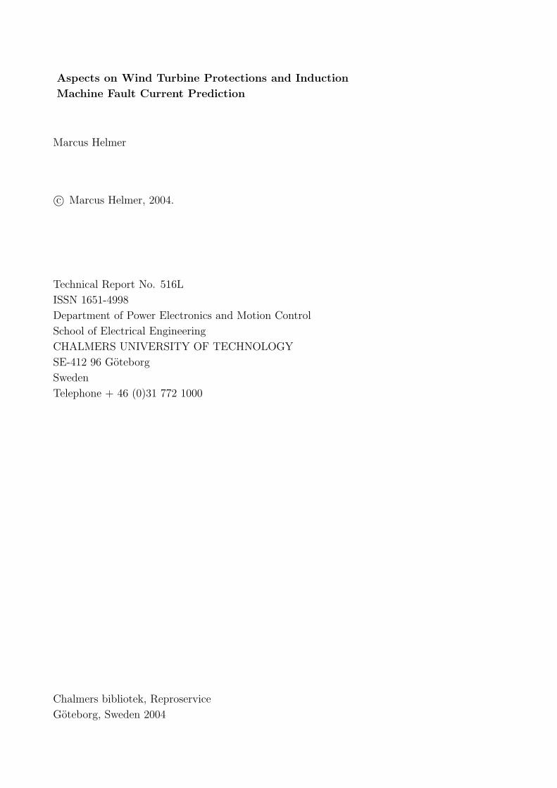
rotor. This is shown in Fig. 5.11.

36

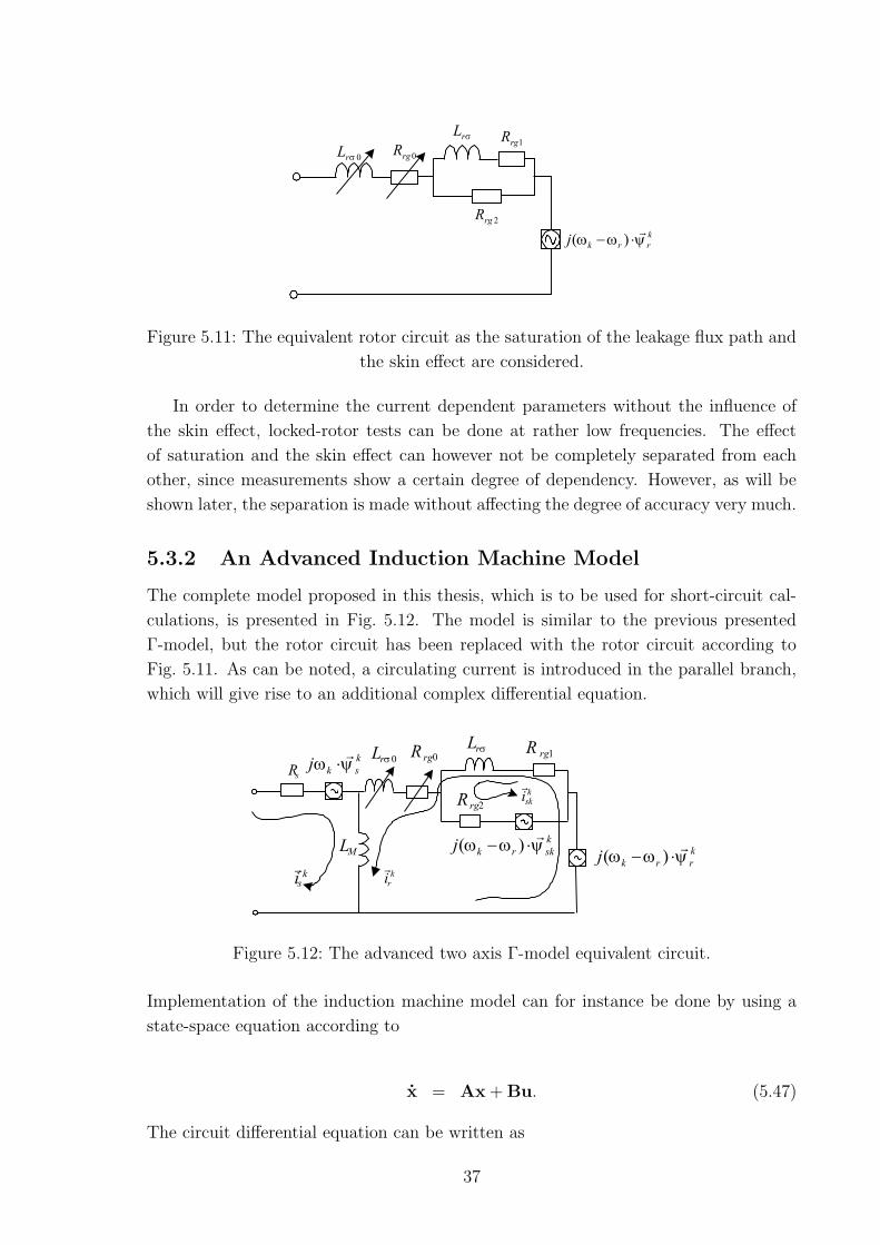
Figure 5.11: The equivalent rotor circuit as the saturation of the leakage flux path and

the skin effect are considered.

In order to determine the current dependent parameters without the influence of

the skin effect, locked-rotor tests can be done at rather low frequencies. The effect

of saturation and the skin effect can however not be completely separated from each

other, since measurements show a certain degree of dependency. However, as will be

shown later, the separation is made without affecting the degree of accuracy very much.

5.3.2 An Advanced Induction Machine Model

The complete model proposed in this thesis, which is to be used for short-circuit cal-

culations, is presented in Fig. 5.12. The model is similar to the previous presented

Γ-model, but the rotor circuit has been replaced with the rotor circuit according to

Fig. 5.11. As can be noted, a circulating current is introduced in the parallel branch,

which will give rise to an additional complex differential equation.

Figure 5.12: The advanced two axis Γ-model equivalent circuit.

Implementation of the induction machine model can for instance be done by using a

state-space equation according to

x = Ax + Bu. (5.47)

The circuit differential equation can be written as

37

U = Rx + Ldx

dt(5.48)

or put in the state-space form

dx

dt= UL−1 − RL−1x (5.49)

where U is a column vector containing input signals, R is the resistance matrix, L is

the inductance matrix and x is a column vector vector representing the continuously

changing variables referred to as states. The vector of input signals, the state vector

and the state vector derivatives can, for the model in Fig. 5.12, be expressed as

U =

uxs

uys

uxr

uyr

uxsk

uysk

Tm

x =

ixsiysixriyrixskiyskωr

dx

dt=

dixsdt

diysdt

dixrdt

diyrdt

dixskdt

diyskdt

dωr

dt

where u represents voltage, i current and Tm the mechanical torque. The superscripts,

x and y, denotes the real and the imaginary part of the two axis vector model respec-

tively. Further, the subscripts s, r and sk denote the stator, the rotor and the skin

effect branch respectively, see Fig. 5.12. The identification of the matrix R and L can

easily be accomplished by means of the fundamental equations, derived and described

in the following.

For an arbitrary reference frame, the stator voltage can according to (5.16) be

expressed as

~uks = Rs

~iks +d~ψk

s

dt+ jωk

~ψks (5.50)

38

Moreover, the rotor voltage can be expressed as

~ukr = (Rrg0 +Rrg1)~i

kr +Rrg1

~iksk +d~ψk

r


kr (5.51)

which looks a bit more complicated than (5.17) due to the incorporation of the skin-

effect phenomenon.

Finally, the additional equation of the skin effect branch is expressed according

~uksk = (Rrg1 +Rrg2)~i

ksk +Rrg1

~ikr +d~ψk

sk


ksk. (5.52)

Further, the flux linkages can be expressed as

~ψks = LM

~iks + LM~ikr (5.53)

~ψkr = LM

~iks + (Lrσ + LM + Lrσ0)~ikr + Lrσ ·~iksk (5.54)

~ψksk = Lrσ

~iksk + Lrσ~ikr (5.55)

and by deriving these three equations we obtain

d~ψks

dt= LM

d~iksdt

+ LMd~ikrdt

(5.56)

d~ψkr

dt= LM

d~iksdt

+ (Lrσ + LM)d~ikrdt

+d(Lrσ0 ·~ikr)

dt+ Lrσ

d~ikskdt

(5.57)

d~ψksk

dt= Lrσ

d~ikskdt

+ Lrσd~ikrdt. (5.58)

As can be noted (5.57) contains the time derivative of the leakage inductance (dLrσ0/dt).

d(Lrσ0 ·~ikr)dt

=dLrσ0

dt~ikr + Lrσ0

d~ikrdt

(5.59)

but by introducing d|ir|/d|ir|, (5.59) can be rewritten as

d(Lrσ0 ·~ikr)dt

= Lrσ0d~ikrdt

+~ikrdLrσ0

d|ir|d|ir|dt

(5.60)

Further, d|ir|/dt can be written as

d|ir|dt

=d

dt

√

(ixr )2 + (iyr)2 (5.61)

39

and if the derivation is performed, the following expression is obtained

d|ir|dt

=ixrdixrdt

+ iyrdiyrdt

|ir|(5.62)

Hence, equation (5.59) can written according to

d(Lrσ0 ·~ikr)dt

= Lrσ0d~ikrdt

+~ikrdLrσ0

d|ir|

[ ixrdixrdt

+ iyrdiyrdt

|ir|

]

(5.63)

which, by separating the equation (5.63) into a real and a imaginary part, can be

expressed in the following way

Lxrσ0 = Lrσ0 +

(ixr )2

|ir|dLrσ0

d|ir|(5.64)

Lyrσ0 = Lrσ0 +

(iyr)2

|ir|dLrσ0

d|ir|(5.65)

Lxyrσ0 =

ixr iyr

|ir|· dLrσ0

d|ir|(5.66)

Finally, the speed equation of the induction machine, which can be expressed ac-

cording to (5.67), where Te is the electromagnetic torque.

Tm = Te −J

p

dωr

dt(5.67)

Te can further be expressed as

Te = p(~ψks (~iks)

∗) (5.68)

where p is number of pole-pairs. ωr is the angular speed expressed in electrical rad/s.

The resistance matrix, R, and the inductance matrix, L, for the advanced two axis

induction machine can finally be identified and expressed according to the following

R =

(Rs −ωkLM 0

ωkLM Rs ωkLM

0 −(ωk − ωr)LM Rrg0 +Rrg1

(ωk − ωr)LM 0 (ωk − ωr)(Lrσ + Lrσ0 + LM)

0 0 Rrg1

0 0 (ωk − ωr)Lrσ

−3

2pLM iry

3

2pLM irx 0

40

−ωkLM 0 0 0

0 0 0 0

−(ωk − ωr)(Lrσ + Lrσ0 + LM) Rrg1 −(ωk − ωr)Lrσ 0

Rrg0 +Rrg1 (ωk − ωr)Lrσ Rrg1 0

−(ωk − ωr)Lrσ Rrg1 +Rrg2 −(ωk − ωr)Lrσ 0

Rrg1 (ωk − ωr)Lrσ Rrg1 +Rrg2 0

0 0 0 0

L =

LM 0 LM 0 0 0 0

0 LM 0 LM 0 0 0

LM 0 Lrσ + LM + Lxrσ0 Lxy

rσ0 Lrσ 0 0

0 LM Lxyrσ0 Lrσ + LM + Ly

rσ0 0 Lrσ 0

0 0 Lrσ 0 Lrσ 0 0

0 0 0 Lrσ 0 Lrσ 0

0 0 0 0 0 0 −Jp

5.3.3 Slip-Ringed Induction Machine

The slip-ringed induction machine is used in the DIFG wind turbine system, Fig. 5.13.

The generator has a wounded rotor supplied by a power electronic converter, which

implies that the rotor voltage can be controlled.

Figure 5.13: Variable-speed doubly-fed induction generator system.

The equations describing the slip-ringed induction machine, is identical with the

general equations describing the squirrel-cage induction machine. The only difference

is that ~ukr 6= 0.

~uks = Rs

~iks +d~ψk

s

dt+ jωk

~ψks (5.69)

~ukr = Rr

~ikr +d~ψk

r


kr . (5.70)

For the slip-ringed induction machine the rotor voltage is adjusted to achieve a

desired slip or torque and the following simplified expressions describes the relationship

41

between the rotor and the stator voltage (~us, ~ur), the slip, s and the torque, Te [1].

The slip can be described according to (5.71)

s =ω − ωr

ω≈ |~ur

~us

| (5.71)

and the torque according to (5.72)

Te = Pmp

(1 − s)ω(5.72)

where p is the number of pole pairs, Pm the mechanical power and ω the synchronous

angular frequency. ωr is the angular frequency of the rotor.

The objective of this thesis is to study the response of severe network fault conditions,

but as the slip-ringed induction machine is considered, even disturbances are of great

interest and importance.

For severe faults, the inverter is protected from over voltages by a crow-bar that

short circuits the rotor windings. The behavior of the slip-ringed induction machine

can therefor be considered similar to that of the squirrel-cage induction machine and

the equations presented in previous section may be used. In Fig. 7.12 a schematic figure

of the DFIG system is presented, indicating the placement of the crowbar short-circuit

device.

Figure 5.14: DFIG system including the crowbar short-circuit device.

However, the crowbar short-circuit device may operate even if the supply voltage

only deviates partly from the rated voltage. Depending on the operating conditions

of the DFIG system, the generator can either be running at super-synchronous or

sub-synchronous speed. If the crowbar operation is initiated, it may lead to a large

consumption of reactive power and high currents due to the acceleration/deacceleration

of the induction generator. This fact has led to that the DFIG is disconnected as soon

as possible, after a crowbar operation has been initiated and the rotor windings have

been short circuited. It should be pointed out that this is a very important problem,

and that the manufacturers are working with a solution which will make at least a

short-term voltage drop ride through possible.

42

5.4 Three Phase Model of the Induction Machine

A three-phase model is more useful then the two-axis representation of the induction

machine when it comes to unsymmetrical operating conditions. Each phase winding

in both stator and rotor are represented separately where the angle displacement be-

tween the windings in both the stator and the rotor are 120 in similarity to the real

machine, see Fig. 5.15. In the two axis representation the angle between the two fictive

perpendicular windings is 90.

Figure 5.15: The three phase representation of a induction machine windings.

The effect of saturation is included in the same way as for the advanced xy-model,

i.e. the saturation in the three different phases are considered to be equal. The sim-

plification imply the possibility to calculate the parameters in the same way as for the

two-axis model, where the derivative, dLrλ/di, is calculated exactly in the same way as

in equation 5.62, implying that a transformation from the three phase system to the

two-axis system is done, using the real and the imaginary components to identify the

accurate parameters. This is however accurate as long as the machine is exposed to

symmetrical operating condition or disturbances.

The skin effect is taken into consideration exactly in the same way as for the two-axis

model, in which a parallel branch of a resistance and two inductances are incorporated

in the rotor circuit, Fig. 5.11.

Each winding has a main inductance, Lh. The mutual inductance between two

phase windings is

M = Lh cos(ϑ) (5.73)

where ϑ is the angle between two windings. Between phase winding a and phase

winding b, ϑ is equal to 2π/3, and between phase winding a and c, the angle is equal

43

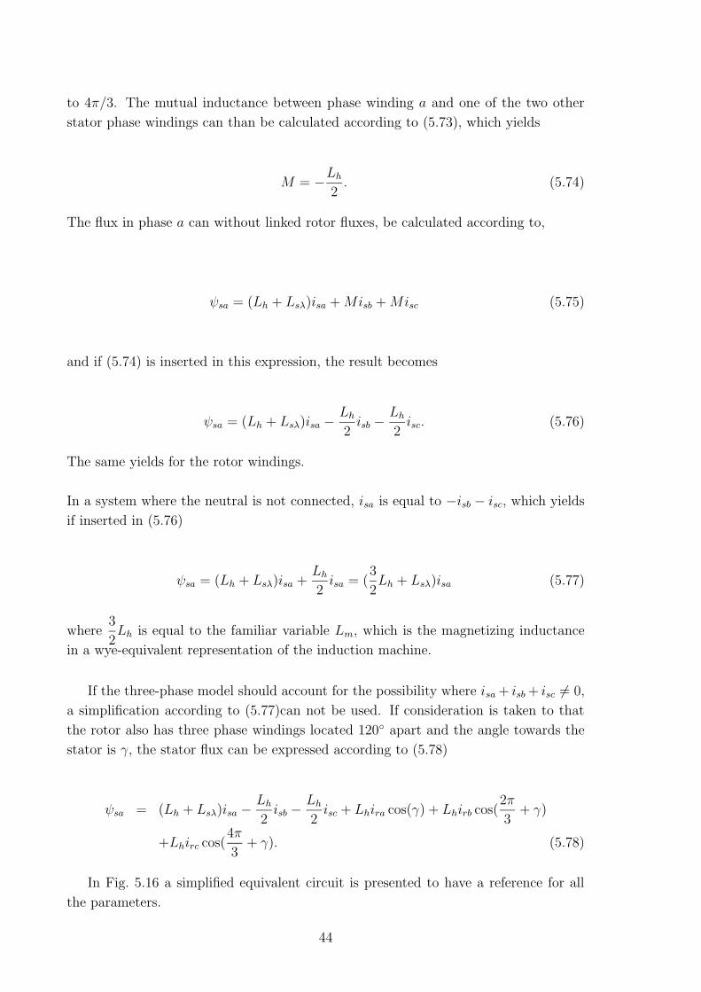
to 4π/3. The mutual inductance between phase winding a and one of the two other

stator phase windings can than be calculated according to (5.73), which yields

M = −Lh

2. (5.74)

The flux in phase a can without linked rotor fluxes, be calculated according to,

ψsa = (Lh + Lsλ)isa +Misb +Misc (5.75)

and if (5.74) is inserted in this expression, the result becomes

ψsa = (Lh + Lsλ)isa −Lh

2isb −

Lh

2isc. (5.76)

The same yields for the rotor windings.

In a system where the neutral is not connected, isa is equal to −isb − isc, which yields

if inserted in (5.76)

ψsa = (Lh + Lsλ)isa +Lh

2isa = (

3

2Lh + Lsλ)isa (5.77)

where3

2Lh is equal to the familiar variable Lm, which is the magnetizing inductance

in a wye-equivalent representation of the induction machine.

If the three-phase model should account for the possibility where isa + isb + isc 6= 0,

a simplification according to (5.77)can not be used. If consideration is taken to that

the rotor also has three phase windings located 120 apart and the angle towards the

stator is γ, the stator flux can be expressed according to (5.78)

ψsa = (Lh + Lsλ)isa −Lh

2isb −

Lh

2isc + Lhira cos(γ) + Lhirb cos(

2π

3+ γ)

+Lhirc cos(4π

3+ γ). (5.78)

In Fig. 5.16 a simplified equivalent circuit is presented to have a reference for all

the parameters.

44

Figure 5.16: Equivalent circuit for the three phase representation, valid for all three

phase quantities.

The stator voltage of phase a, which is familiar from previous chapters, can be

written according to

usa = Rsisa +dψsa

dt. (5.79)

The time derivative of (5.78) can further be expressed as

dψsa

dt= (Lh + Lsλ)

disadt

− Lh

2

disbdt

− discdt

Lh

2− Lhira

dγ

dtsin(γ)

+Lhdira

dtcos γ − Lhirb

dγ

dtsin(

2π

3+ γ) + Lh

dirb

dtcos(

2π

3+ γ)

−Lhircdγ

dtsin(

4π

3+ γ) + Lh

dirc

dtcos(

4π

3+ γ) (5.80)

where dγ/dt = wr. For simplicity, the following variables are now introduced

B1 = sin(γ) A1 = cos(γ)

B2 = sin(2π/3 + γ) A2 = cos(2π/3 + γ)

B3 = sin(4π/3 + γ) A3 = cos(4π/3 + γ)

and finally, the stator and rotor equations can then be expressed according to

usa = Rsisa −XhB1ira −XhB2irb −XhB3irc + (Lsλ + Lh)disadt

− Lh

2

disbdt

−Lh

2

discdt

+ A1Lhdira

dt+ A2Lh

dirb

dt+ A3Lh

dirc

dt(5.81)

usb = Rsisb −XhB3ira −XhB1irb −XhB2irc + (Lsλ + Lh)disbdt

− Lh

2

disadt

−Lh

2

discdt

+ A3Lhdira

dt+ A1Lh

dirb

dt+ A2Lh

dirc

dt(5.82)

usc = Rsisc −XhB2ira −XhB3irb −XhB1irc + (Lsλ + Lh)discdt

− Lh

2

disadt

−Lh

2

disbdt

+ A2Lhdira

dt+ A3Lh

dirb

dt+ A1Lh

dirc

dt(5.83)

45

ura = −XhB1isa −XhB3isb −XhB2isb + (Rrg0 +Rrg1)ira +Rrg1iska + A1Lhdisadt

+A3Lhdisbdt

+ A2Lhdiscdt

+ (Lrσ + Lh)dira

dt+d(Lrσ0 · ira)

dt− Lh

2

dirb

dt

−Lh

2

dirc

dt+ Lrσ

diska

dt(5.84)

urb = −XhB2isa −XhB1isb −XhB3isb + (Rrg0 +Rrg1)irb +Rrg1iskb + A2Lhdisadt

+A1Lhdisbdt

+ A3Lhdiscdt

+ (Lrσ + Lh)dirb

dt+d(Lrσ0 · irb)

dt− Lh

2

dira

dt

−Lh

2

dirc

dt+ Lrσ

diskb

dt(5.85)

urc = −XhB3isa −XhB2isb −XhB1isb + (Rrg0 +Rrg1)irc +Rrg1iskc + A3Lhdisadt

+A2Lhdisbdt

+ A1Lhdiscdt

+ (Lrσ + Lh)dirc

dt+d(Lrσ0 · irc)

dt− Lh

2

dira

dt

−Lh

2

dirb

dt+ Lrσ

diskc

dt(5.86)

Further, the equations for representing the skin effect branch can be expressed as

uska = Rrg1ira + (Rrg1 +Rrg2)iska + Lrσdira

dt+ Lrσ

diiska

dt

uskb = Rrg1irb + (Rrg1 +Rrg2)iskb + Lrσdirb

dt+ Lrσ

diiskb

dt(5.87)

uskc = Rrg1irc + (Rrg1 +Rrg2)iskc + Lrσdirc

dt+ Lrσ

diiskc

dt(5.88)

(5.89)

The electromagnetic torque for the three-phase induction machine model can be

written as

Te = −pLh

(

(B1ira +B2irb +B3irc) + (B1irb +B2irc +B3ira) +

(B1irc +B2ira +B3irb))

(5.90)

All these equations presented above results in the following resistance matrix

46

Rs 0 0

0 Rs 0

0 0 Rs

−XhB1 −XhB3 −XhB2



0 0 0

0 0 0

0 0 0

−pLh(B1ira +B2irb +B3irc) −pLh(B1irb +B2irc +B3ira) −pLh(B1irc +B2ira +B3irb)

0 0 0

−XhB1 −XhB2 −XhB3 0 0 0 0 0

−XhB3 −XhB1 −XhB2 0 0 0 0 0

−XhB2 −XhB3 −XhB1 0 0 0 0 0

Rrg1 +Rrg0 0 0 Rrg1 0 0 0 0

0 Rrg1 +Rrg0 0 0 Rrg1 0 0 0

0 0 Rrg1 +Rrg0 0 0 Rrg1 0 0

Rrg1 0 0 (Rrg1 +Rrg2) 0 0 0 0

0 Rrg1 0 0 (Rrg1 +Rrg2) 0 0 0

0 0 Rrg1 0 0 (Rrg1 +Rrg2) 0 0

0 0 0 0 0 0 0 0

0 0 0 0 0 0 −1 0

and the following inductance matrix

(Lsλ + Lh) −Lh/2 −Lh/2 A1Lh A2Lh

−Lh/2 (Lsλ + Lh) −Lh/2 A3Lh A1Lh

−Lh/2 −Lh/2 (Lsλ + Lh) A2Lh A3Lh

A1Lh A3Lh A2Lh (Lrσ0 + Lh + Lrσ + LσAira) LσBira − Lh/2

A2Lh A1Lh A3Lh LσAirb − Lh/2 (Lrσ + Lh + Lrσ0 + LσBirb)

A3Lh A2Lh A1Lh LσAirc − Lh/2 LσBirc − Lh/2

0 0 0 Lrσ 0

0 0 0 0 Lrσ

0 0 0 0 0

0 0 0 0 0

0 0 0 0 0

47

A3Lh 0 0 0 0 0

A2Lh 0 0 0 0 0

A1Lh 0 0 0 0 0

LσCira − Lh/2Lrσ 0 0 0 0

LσCirb − Lh/2 0 Lrσ 0 0 0

(Lrσ + Lh + Lrσ0 + LσCirc) 0 0 Lrσ 0 0

0 Lrσ 0 0 0 0

0 0 Lrσ 0 0 0

Lrσ 0 0 Lrσ 0 0

0 0 0 0 −J/p 0

0 0 0 0 0 1

where LσA, LσB and LσC are the results from the derivation of the terms d(Lσ0·dira)/dt,d(Lσ0 · dirb)/dt and d(Lσ0 · dirc)/dt in (5.84), (5.85) and (5.86). All according to the

same procedure as in (5.59) - (5.66), which is again is presented below.

d(Lrσira)

dt= Lrσ · dira

dt+ ira ·

dLrσ

dt(5.91)

dLrσ

dt=

dLrσ

d|ir| ·d|ir|dt

(5.92)

where d|ir|/dt can be described according to (in accordance with (5.8)

d|ir|dt

=d

dt

√

i2ra +1

3

(

irb − irc

)2(5.93)

=d

dt

√

i2ra +1

3

(

i2rb − 2irbirc + i2rc

)

=1

2|ir|·[

2iradira

dt+

2

3irbdirb

dt− 2

3

(

irbdirc

dt+ irc

dirb

dt

)

+2

3ircdirc

dt]

=ira

|ir|dira

dt+

1

3

(irb − irc)

|ir|dirb

dt+

1

3

(irc − irb)

|ir|dirc

dt.

Finally, LσA, LσA and LσA, can be written according to

LσA = [Lrσ +i2ra

|ir|dLrσ

d|ir|] (5.94)

LσB = [1

3

(irb − irc)ira

|ir|dLrσ

d|ir|] (5.95)

LσC = [1

3

(irc − irb)ira

|ir|dLrσ

d|ir|]. (5.96)

48

Chapter 6

Experimental set-up and Parameter

Identification

In the previous chapter was described how the machine parameters vary due to skin

effect and leakage flux saturation and how these two phenomena could be incorporated

into the models, in order predict the dynamic behavior and the fault current response.

Unfortunately there is no shortcut when it comes to determining the parameters and

how the parameters vary due to changing current and frequency. As mentioned earlier,

one has to either accomplish advanced FEM computations, with respect to the geo-

metrical design of the generator, or perform extensive measurements, which have been

done in this thesis.

There are mainly three different experimental set-ups that have been used. One

for steady-state measurements, which has been used for the parameter identification

of the induction machine and one for dynamic measurements which was used in order

to apply disturbances to the induction machine. Finally, an experimental set-up for

the investigation of the response of the slip-ringed induction machine, due to network

disturbances and resulting crow-bar action, has been used.

Since the objective of the thesis is to predict the currents arising from severe fault

conditions, the rotor and stator resistances and the leakage inductances are of great

interest. To account for phenomena, such as skin effect and saturation of the leakage

flux path, the tests have to be done for different frequencies and voltage (current) levels

respectively.

6.1 Steady State Measurements

To identify the steady state parameters of an induction machine, a no-load test, a

locked-rotor test and measurement of the stator resistance have to be made. For many

cases where an induction machine model is needed, one set of parameters valid for

50Hz and rated current are satisfactory. However, for advanced calculations a more

detailed model, such as the model presented in chapter 5 can be required and as already

49

been mentioned, the identification measurements become more extensive. In Fig. 6.1

the connection used for the parameter identification is presented. The connection

is used for symmetrical three phase measurements (besides three phase short circuit

measurements), such as starts, locked rotor tests and no-load tests.

Fuse box

Resistances

Measurement box

Auto-transformers

PC

Induction machine

Voltage Source,

10-100Hz, 0-400V

Figure 6.1: The measurement setup for steady state measurements.

The voltage sources have been of different types. To start with, the strong 50Hz

230V and 400V grid, were used. These two different voltage levels are obtained by

transformation from the 10kV distribution network, with no other separate objects

connected, apart from the induction machine. Resistors connected in series were in

this case used to provide the possibility to adjust the voltage level. For some cases

auto-transformers were used to obtain various voltages at the fixed frequency of 50Hz.

An electrically magnetized speed controlled synchronous machine was used at some

occasions, which had the advantage that a voltage with a very low harmonic distortion

could be delivered and it could also provide us with the possibility to change the

frequency as well as the voltage magnitude in a broad range. A drawback however,

was the inability of the synchronous machine to maintain a constant voltage magnitude

during transient fault conditions and it was thus only useful for steady state parameter

50

identification measurements.

The measurement interface consist of voltage and current transducers, AD210 BN

and LEM-modules with a bandwidth of several kHz. The sampling frequency was set

to 5 kHZ.

In Fig. 6.2 - Fig. 6.5 pictures of the different components in the measurement set-up

are shown.

Figure 6.2: Three phase resistances that sometimes were used to limit the applied

voltage.

Figure 6.3: The photo show the auto-transformers. The 200A input connections can

be noted on the short side of the auto-transformers and the different levels of out-put

voltage can be noted on the front side on the autotransformer in the middle of the

picture.

51

Figure 6.4: Fuse box used to protect the bigger more expensive fuses that protects the

voltage sources.

Figure 6.5: Measurement box with the LEM modules for current measurement. The

box also includes the voltage measurement cards (not shown in the picture).

Steady-state measurements have been performed on a 15kW squirrel -cage induction

machine and on a 22kW slip-ringed induction machine, where the 15kW induction

machine has been used as the main object. The manufacturer data of the 15kW

machine is presented in Table 6.1 and the machine is shown in Fig. 6.6.

52

Table 6.1: General parameter values given by the manufacturer for the 15kW squirrel-

cage induction machine.

Rs Stator resistance 0, 18Ω

Rr Rotor resistance 0, 19Ω

Lm Magnetizing inductance 42, 6mH

Lsλ Stator leakage inductance 2, 55mH

Lrλ Rotor leakage inductance 2, 07mH

J Inertia 0, 205kgm2

Un Rated voltage 380V

f Frequency 50Hz

p Number pole pairs 3

n Nominal speed 970rpm

Figure 6.6: A picture of the 15kW squirrel-cage induction machine.

The same parameters for the 22kW slip-ringed induction machine is presented in

Table 6.2 and a photo of the 22kW slip-ringed induction machine is presented in Fig. 6.7

53

Table 6.2: General parameter values given by the manufacturer for the 22kW slip-ringed

induction machine.

Rs Stator resistance 0, 115Ω

Rr Rotor resistance 0, 184Ω

Lm Magnetizing inductance 46, 6mH

Lsλ Stator leakage inductance 1, 65mH

Lrλ Rotor leakage inductance 1, 68mH

J Inertia 0, 534kgm2

Un Rated voltage 400V

f Frequency 50Hz

p Number of pole pairs 2

n Nominal speed 1440rpm

Figure 6.7: A picture of the 22kW slip-ringed induction machine also showing the DC

machine.

The parameters presented in the tables above are related to the conventional T-

model or the Park model. A simple equivalent circuit is presented in Fig. 6.8, where

all the parameters given by the manufacturer are shown.

54

Figure 6.8: Classical equivalent circuit of the induction machine.

6.1.1 No Load Test

The no-load test is accomplished by applying voltage to the induction machine, which

will start to rotate. When the machine has reached the final speed, the voltages and the

currents are measured in each phase. From this kind of measurement the magnetizing

inductance can be determined as a function of the no-load voltage (its variation has

however a little influence on the dynamic behavior of the induction machine). In Table

6.3 LM is presented together with the no-load voltage, the no-load current and the flux

in p.u.. Note that the measurement is made at 40Hz, which was done to reach a higher

flux level without exceeding the nominal voltage of the machine too much. In Fig. 6.9

the magnetizing inductance is presented as a function of the applied stator flux.

Table 6.3: No load test of MK171012-AA at 40Hz.

Voltage (V ) Current (A) Flux (p.u.) LM (H)

95,5 5,26 0.3140 0,04119

142,8 7,85 0.4695 0,0415

189,6 10,67 0.6234 0,0406

236,5 13,77 0.7776 0,0393

283,5 17,93 0.9321 0,0362

302,5 20,16 0.9946 0,0343

321,4 22,95 1.0567 0,0321

340,2 26,41 1.1185 0,0295

359,5 30,85 1.1820 0,0267

368,8 33,40 1.2126 0,0253

378,3 36,30 1.2438 0,0239

387,8 39,50 1.2750 0,0225

397,3 43,19 1.3063 0,0211

406,6 47,34 1.3369 0,0197

55

0.4 0.6 0.8 1 1.20.015

0.02

0.025

0.03

0.035

0.04

0.045

Flux (p.u.)

Indu

ctan

ce (H

)

Figure 6.9: The magnetizing inductance as a function of the flux.

It can be noted in the table above that the magnetizing inductance varies with the

applied stator flux. However, as a severe fault occurs, a very small amount of the short

circuit current will run through the magnetizing inductance. In Fig. 6.10 and Fig. 6.11

the short circuit parameters of the Γ-model are presented using measurement where a

fixed (nominal) and a variable magnetizing inductance has been used.

0 50 100 150 200 2502.5

3

3.5

4

4.5

5x 10

−3

Stator current magnitude (A)

Lσ (H

)

Figure 6.10: The rotor inductance of the Γ-model at a fixed magnetizing inductance

according to Table 6.1 (solid) and a varying magnetizing inductance according to Table

6.3 (dashed).

56

0 50 100 150 200 2500.25

0.3

0.35

0.4

Stator current magnitude (A)R

rg (Ω

)

Figure 6.11: The rotor resistance of the Γ-model at a fixed magnetizing inductance

according to Table 6.1 (solid) and a varying magnetizing inductance according to Table

6.3 (dashed).

From Fig. 6.10 and Fig. 6.11 it can be observed that the importance of accounting

for a variable magnetizing inductance when determining the short circuit parameters

of the induction machine is very low.

6.1.2 Locked Rotor Test

The manufacturer general parameters do not imply any consideration to the varying

character of the rotor parameters with respect to the frequency or the current. A

detailed data sheet from the manufacturer may be available sometimes, which opens

up the possibility to at least roughly incorporate for saturation of the leakage flux path

and skin effect without performing extensive measurements. In this thesis however,

locked-rotor tests at both different frequencies and voltage levels have been performed.

Skin Effect

Considering the skin effect, the influence on the stator parameters are not as large as

the influence on the rotor parameters. The stator conductors are relatively thin (ap-

proximately 1.9 mm2 for the 15kW induction machine), and the stator resistance is not

affected by the skin effect around 50 Hz and below. This is related to the penetration

depth of the magnetic field, into the current carrying conductors and accordingly the

stator resistance is kept constant.

The skin depth can be calculated according to [3]

δ =1√πfµσ

(6.1)

where f is the frequency, µ the permeability (µ = µ0µr, where µ0 = 4π−7) and σ the

conductivity of the conductor material. The permeability and the conductivity for the

two most common conductor materials and iron are presented in Table 6.4.

57

Table 6.4: Skin depths (mm) of various materials.

Material µr σ

Copper ∼1 59,6·106 mΩ

Aluminum ∼1 37, 7·106 mΩ

Iron ∼103 10,3·106 mΩ

In Table 6.5 the different skin depths of copper, aluminium and iron is presented

calculations are made using (6.1) and the values according to the table above.

Table 6.5: Skin depths (mm) of various materials.

Material 10Hz 50Hz 100Hz

Aluminum 25,9 11,6 8,2

Copper 20,6 9,2 6,5

Iron 1,57 0,70 0,49

Saturation

A good way to illustrate saturation is the B-H curve, Fig. 6.12, which shows the effect

of applying a magnetic field to un-magnetized iron. The magnetizing curve starts at

the origin (0,0) and increases linearly as the magnetic field magnetizes the iron (observe

that the hysteresis has been neglected in the figure).

Figure 6.12: B-H curve illustrating the phenomena of saturation.

Eventually, however, all the magnetic domains align with the applied field, and the

curve flattens out as the iron becomes magnetically saturated. This is what happens

as the current running through the conductors increase. The increasing magnetic field

around the conductors saturates the iron around the rotor slots of the machine.

58

6.1.3 Rotor Parameter determination

With the knowledge of the stator resistance, the magnetizing inductance and the no-

load inductance, the leakage inductance as well as the rotor resistance for the Γ-model

can be determined using equations (5.35) and (5.36). Table 6.6 and 6.7 presents the

leakage inductance (which is the same as the rotor leakage-inductance for the Γ-model),

(Lσ) and the rotor resistance (Rrg), from the locked rotor tests at different current and

frequency levels. It can be noted that the parameters vary with frequency as well as

with current magnitude.

Table 6.6: Lσ(mH) for different frequencies and stator currents (RMS-values).

Hz 60 A 90 A 120 A

10 4.17 3.70 3.36

15 4.16 3.67 3.31

20 4.14 3.66 3.30

30 4.09 3.627 3.27

40 4.06 3.59 3.23

50 4.01 3.55 3.19

60 3.96 3.50 3.13

80 3.83 3.36 3.03

100 3.66 3.18 2.92

Table 6.7: Rrg(Ω) for different frequencies and stator currents(RMS-values).

Hz 60 A 90 A 120 A

10 0.210 0.202 0.197

15 0.218 0.209 0.208

20 0.229 0.229 0.212

30 0.250 0.246 0.231

40 0.295 0.278 0.254

50 0.337 0.312 0.303

60 0.384 0.359 0.370

80 0.500 0.505 0.471

100 0.642 0.602 0.596

In Fig. 6.13 and in Fig. 6.14 the values from the tables above are presented in two

graphs. It is now easy to identify the changes due to different current levels as well as

due to varying frequencies.

59

20 40 60 80 1002.8

3

3.2

3.4

3.6

3.8

4

x 10−3

Frequency (Hz)

Lσ (m

H)

Figure 6.13: The short circuit inductance as a function of frequency at different current

levels. The current level is increasing going from the top in the figure to the bottom,

∗ = 60A,× = 90A and + = 120A.

20 40 60 80 100

0.2

0.3

0.4

0.5

0.6

Frequency (Hz)

Rrg

(Ω)

Figure 6.14: The short circuit resistance as a function of frequency at different current

levels, ∗ = 60A,× = 90A and + = 120A.

As can be noted in Fig. 6.13, the short circuit inductance does not depend on the

frequency very much, whereas the short circuit resistance is highly dependent as can

be noted in Fig. 6.14. The current level affects the leakage inductance while it has a

very little effect on the resistance.

In Table 6.8 the measured leakage inductance, Lσ, and the rotor resistance, Rrg, of

the Γ-model is presented as a function of the current magnitude at a fixed frequency

of 50Hz, where the effect of saturation is evident.

60

Table 6.8: Locked rotor test at 50Hz. Voltage source IR and T12

Stator current (A) Lσ (mH) Rrg (Ω)

6.6 4.433 0.381

13.5 4.520 0.381

17.1 4.542 0.381

23.6 4.554 0.381

30.2 4.534 0.377

37.1 4.477 0.372

44.4 4.386 0.365

59.4 4.017 0.337

90.6 3.551 0.312

120.2 3.194 0.303

197.7 2.831 0.295

244.1 2.616 0.287

280.0 2.498 0.280

301.5 2.433 0.283

310.6 2.411 0.282

395.9 2.248 0.282

429.0 2.164 0.262

To separate the stator and the rotor leakage inductances is practically impossible

for a squirrel-cage induction machine, but the distribution between the rotor- and the

stator leakage inductance is of minor importance for the dynamic performance of the

machine, as long as the total leakage inductance is correct. This emphasizes the use

of the Γ-model, which only contains one leakage inductance. The Γ-model equivalent

circuit is presented in Fig. 6.15.

Figure 6.15: Simple equivalent circuit of the Γ-model.

The rotor resistance and the rotor leakage inductance can be calculated for differ-

ent frequencies resulting in a relationship between those two, which is represents in

Fig. 6.16.

61

0.2 0.3 0.4 0.5 0.6 0.7 0.80

0.5

1

1.5

2

2.5

3

Rotor resistance (Ω)

Lea

kage

reac

tanc

e (Ω

)←10 Hz

←15 Hz←20 Hz

←30 Hz

←40 Hz←50 Hz

60 Hz→

←80 Hz

←100 Hz

Figure 6.16: Rotor circuit impedance where circles indicate measurements, dots rep-

resents the rotor configuration according to Fig. 5.5 and Solid line represents a rotor

circuit configuration according to Fig. 5.7.

Both the leakage flux path saturation and the skin effect are both rather simple to

account for separately.

To make a rotor equivalent circuit that accounts for both these effects simultane-

ously seems to be very difficult and perhaps not worthwhile if ”cost” is considered with

respect to the calculation of the parameters and simulation time when the model is

used. In this thesis the following more simple approach has been used and is believed

to be adequate.

As these two effects shall be combined one current level for which the skin effect

shall be represented has been chosen. In our case a medium current level ( 90A) has

been chosen. One advantage, is that the characteristics of the frequency dependent

inductance more or less follow the same pattern, regardless of the current level. The

total rotor impedance has after the selection of current level been divided into two

paths, one that accounts for the leakage flux path saturation and one that accounts for

the skin effect.

Fig. 6.17 show the parameters of the rotor circuit, where the two parts, the skin

effect representation (to the right) and the representation of the leakage flux path

saturation is shown.

Figure 6.17: The equivalent rotor circuit as the saturation of the leakage flux path and

the skin effect are considered.

62

The resistances are also dependent on the temperature. This factor was eliminated

by measurements of the temperature in one of the rotor and the stator windings. By

leaving the machine to cool down between the tests the temperature could be held

constant. The measured temperature was in this way kept within in a range of 22-27

degrees Celsius.

6.2 Dynamic measurement I - Grid Connection

The measurement set-up for the dynamic measurements were slightly different com-

pared to the previous set-up. It consists of resistances, auto-transformers and the

measurement interface, which are the same as for the steady-state measurement set-

up. The voltage source however, is only the 50Hz, fixed voltage connections, since the

synchronous generator was unable to provide a stable supply voltage during the applied

fault conditions. In Fig. 6.18 the measurement set-up for short circuit measurements

is presented. As can be noted a short circuit device has been added, which has the

possibility to short circuit two or three phases. In Fig. 6.19 a photo of the short circuit

device is presented. The different faults were created on the secondary side of the

contactor, so for a three phase short circuit fault all three phases were short circuited.

The purpose of the dynamic measurements are to create realistic faults, applied to

the terminals of the machine, in order to verify the mathematical models presented in

the previous chapters. The primarily applied faults are three phase short circuit faults,

which are considered the most severe, and will expose the machine to very high current

levels. In the following chapters measurements and simulations will be compared.

63

Fuse box

Resistances

Measurement box

Auto-transformers

PC

Induction machine

Voltage Source,

50Hz, 230/400V

Short circuit

device

Figure 6.18: The experimental set-up for short circuit measurements.

64

Figure 6.19: The short circuit contactor which is used to short circuit the three phases

feeding the induction machine.

6.3 Dynamic Measurement II - Crow-bar operation

Crow-bar operation is related to DFIG systems, which are a bit more sensitive than a

fixed speed generator system, since it embraces a converter between the rotor windings

and the grid. During fault conditions, the current limitations of the converters can be

exceeded. The rotor circuit is then short circuited by means of a crow-bar, in order

to protect the converter. At this point of operation the slip-ringed induction machine

can be described in the exact same way as the squirrel-cage induction machine, but

with a non-natural operating point, initially. The measurements have in this case been

performed on a 22kW slip-ringed induction machine.

The experimental set-up for this case, is rather complicated and includes a DC

machine with a thyristor rectifier/inverter controlling the torque, a slip-ringed induction

machine with resistors emulating the rotor converter and the short circuiting crow-bar.

Moreover, a thyristor converter that could generate voltage dips and maintain a stable

voltage, regardless of the current level, is used. In this set-up, the current levels had

to be kept to a moderate level in contradiction to the previous one, where more brutal

tests could be conducted. In Fig. 6.20 the connection is presented and in Fig. 7.15 a

picture of the crow-bar set-up is shown.

65

crow-bar

Resistors

DC Machine 22kW Ind. Machine

Toruqe controller

Converter with dip generating

function

Torque transducerDC Source

Figure 6.20: A picture of the measurement set-up for measurements of crow-bar oper-

ation.

Figure 6.21: The picture shows the crow-bar which short circuits the rotor windings in

case of a voltage dip.

The crow-bar consisted of a three-phase diode rectifier with a large IGBT transistor

on the dc side. When the rotor current level reached a triggering level, the IGBT was

turned on which lead to a short-circuit of the rotor windings.

66

Chapter 7

Model Verification

All models presented in this thesis can be used for analysis of symmetrical disturbances

or faults, although the accuracy of the result varies due to the complexity of the model

used. The experimental verification of the models is made comparing simulations and

measurements, from locked rotor tests, starts and three-phase short-circuits. The com-

parisons are made with results from simulations using the traditional fifth order Park

model and measured parameters according to the standard locked-rotor and no-load

test. Comparisons are also made using the manufacturer general parameters and finally

comparisons using the advanced model are presented.

In the following sections, the magnitude of the absolute value of the stator current is

usually presented, in order to facilitate the comparisons. The advantage of presenting

the stator current magnitude, is that different cases can be compared more easily. The

reason for this is that the peak current level, looking at one stator phase current, can

differ around 10%, depending on the voltage angle at the time instant of the three-

phase short circuit, while the total stator current magnitude is independent of the

voltage angle at the time the fault occurs. In Fig. 7.1 the phase current magnitude as

a function of the voltage angle, α, is presented.

0 10 20 30 40 50 600

0.2

0.4

0.6

0.8

1

Voltage phase angle, α

Max

. sta

tor p

hase

cur

rent

mag

.

Figure 7.1: The maximum stator phase current magnitude as a function of the voltage

angle.

67

A voltage angle, α, equal to zero corresponds to a three phase short circuit occurring

at the time when one of the phase voltages is crossing zero.

7.1 Three Phase Locked Rotor Test

In Fig. 7.2 a locked rotor test at 230 V is presented. The figure shows the stator cur-

rent magnitude originating from the measurement, the simulation results from using

the advanced induction machine model and the same results from using the conven-

tional T -model, when the manufacturer general parameters are used as well as when

the parameters are tuned for the specific case. As can be noted, the proposed model

predicts excellent result. Worth noticing is the poorly predicted result by the conven-

tional T-model using the manufacturer’s parameters, even as the steady-state condition

is reached at the end of the time series. An improvement can be made by tuning the pa-

rameters of the T-model with respect to the specific current level, i.e. using calculated

parameters from a conventional no-load and a specific locked-rotor test made at the

specific current level. However, the initial transient processes is still poorly predicted

with this method.

0.6 0.61 0.62 0.63 0.64 0.650

50

100

150

200

250

Time (s)

Cur

rent

(A)

Figure 7.2: Locked-rotor test at 230 V. Solid line show the measurement, dashed line

show the advanced model, dashed-dotted line show the T-model with tuned param-

eters and dotted line show the T-model with the parameters according to standrd

manufacturer data.

Fig. 7.3 shows the three-phase currents from the previous case and as can be noted the

prediction of the advanced model is as in the previous case very good.

In Fig. 7.4 a locked-rotor test at rated voltage is presented. The same comments

that are made for Fig. 7.3, can be made also for this case, but as can be noted the

prediction fails slightly as the current raises above 500 A. This is due to limitations of

the experimental setup, which made it impossible to have 500A for a time long enough

to identify the short circuit parameters. To try to identify the parameters over 500

A, could very well have destroyed the machine as well as other equipment. Higher

current levels could perhaps have been obtained by blocking the protection systems

68

0.6 0.61 0.62 0.63 0.64 0.65

−200

−100

0

100

200

Time (s)Ph

ase

curr

ent (

A)

Figure 7.3: Locked-rotor test at 230 V. Solid line show the advanced model and dashed

line show the measurement.

and changing to larger fuses in the internal power supply of the laboratory, but was

not considered necessary since the modelling strategy proved to work extremely well

for the 230V case.

0.16 0.18 0.2 0.22 0.24 0.260

100

200

300

400

500

600

Time (s)

Phas

or m

agni

tude

(A)

Figure 7.4: Locked-rotor test at 400 V. Solid line show the measurement, dashed line

show the advanced model, dashed-dotted line show the T-model with tuned parameters

and dotted line show the T-model with the parameters according to manufacturer data.

7.2 Start

Starting the induction machine by connecting it directly to the grid imply that the

machine is subjected to a quit high current initially due to the magnetization and

acceleration of the rotor. This current has a magnitude in the range of approximately

7 - 10 times rated current. As the machine in this case is started without load, the

starting time is quite short and the high current decays rather quickly.

Fig. 7.5 shows the absolute value of the current from a start at 230 V and Fig. 7.6

shows the three-phase currents.

69

0.45 0.5 0.550

50

100

150

200

250

Time (s)

Cur

rent

(A)

Figure 7.5: A start at 230 V. Solid line show the measurement, dashed line show the

advanced model, dashed-dotted line show the T-model with tuned parameters and

dotted line show the T-model with the parameters according to manufacturer data.

0.45 0.5 0.55

−200

−100

0

100

200

Time (s)

Phas

e cu

rren

t (A

)

Figure 7.6: A start at 230 V. Solid line show the advanced model and dashed line show

the measurement.

In Fig. 7.7 a comparison between the measurements, the conventional T-model,

with the manufacturers general parameters and with tuned parameters, as well as the

advanced model is presented. It is again evident that an advanced model predicts the

currents very well compared to the prediction by the traditional T-model, which does

not predict a very good result.

70

0.15 0.2 0.25 0.30

100

200

300

400

500

600

Time (s)St

ator

cur

rent

mag

nitu

de (A

)

Figure 7.7: Start of the induction machine at rated voltage (400 V). Solid line show

the measurement, dashed line show the advanced model, dashed-dotted line show the

T-model with tuned parameters and dotted line show the T-model with the parameters

according to manufacturer data.

7.3 Three Phase Short Circuit Fault

During a three-phase short circuit the machine is de-energized and subjected to currents

with a magnitude in the same range, as the machine is subjected to at a start (direct

start).

In Fig. 7.8 a three-phase short circuit is presented at 230 V. It shows the predic-

tion by the advanced model and the T-model with the parameters according to the

manufacturer and as well as the parameters adjusted for the specific case.

0.16 0.18 0.2 0.22 0.24 0.260

50

100

150

200

250

Time (s)

Cur

rent

(A)

Figure 7.8: A three phase short circuit test at 230 V. Solid line show the measurement,

dashed line show the advanced model, dashed-dotted line show the T-model with tuned

parameters and dotted line show the T-model with the parameters according to man-

ufacturer data.

Fig. 7.9 shows the same case, but presents the three-phase currents.

71

0.16 0.18 0.2 0.22 0.24 0.26

−200

−100

0

100

200

Time (s)

Phas

e cu

rren

t (A

)

Figure 7.9: Short circuit at 230 V. Solid line show the advanced model and dashed line

show the measurement.

To really verify the model presented in this thesis, the machine has been subjected

to full or rated voltage short circuits. In Fig. 7.10 the absolute value of the current

predicted by the advanced model and the T-model. For the T-model, two sets of pa-

rameters have been used; The manufacturer general parameters and a set of parameters

adjusted to fit this specific case (The parameters given from a full-voltage locked-rotor

test).

0.88 0.9 0.92 0.94 0.96 0.98 10

100

200

300

400

500

Time (s)

Stat

or c

urre

nt m

agni

tude

(A)

Figure 7.10: Short circuit fault applied on the 15kW squirrel-cage induction machine

at 400 V. Solid line show the measurement, dashed line show the advanced model,

dashed-dotted line show the T-model with tuned parameters and dotted line show the

T-model with the parameters according to manufacturer data.

In Fig. 7.11 the three-phase currents are presented for the same case.

72

0.88 0.9 0.92 0.94 0.96 0.98 1−400

−200

0

200

400

Time (s)Ph

ase

curr

ents

(A)

Figure 7.11: Short circuit fault applied on the 15kW squirrel-cage induction machine

at 400 V. Solid line shows the advanced model and dashed line the measurement.

As can be noted in the above presented comparisons, the agreement between mea-

surements and the advanced model is excellent.

7.3.1 IEC 909 Comparison

In Chapter 4 the short circuit calculation procedure for induction machine was pre-

sented. The parameters according to the manufacturer was used and the initial short

circuit current as well as the peak short circuit current were calculated. The peak

short current which is the highest current level during a short circuit and the absolute

highest value can be seen during three phase short circuits.

For the 15kW squirrel-cage induction machine the peak short circuit current was

calculated to 451A, which is to be compared with peak current value according to the

measurement and the simulation in Fig. 7.11. The measurement and the simulation

shows a result of approximately 370A, so the IEC standard provides a somewhat high

result. This is of course better than if the result would be to low, but as large generators

and wind farms are put up and used for calculating the fault currents, this can be

associated with high costs. The dimensioning of substations are dependent on the

short circuit currents and going from one short circuit level to a higher one can be very

expensive. Circuit breakers, fuses, busbars and all other equipment must be able to

withstand the forces due to a three phase short circuit.

7.4 DFIG-System

When severe disturbances are considered, the fault response of a doubly-fed induction

machine is similar to the response of the short-circuited induction machine, but it also

be worse, depending on the point of operation at the time before the fault and the crow

bar operation. If the current limitation of the inverter connected to the rotor circuit of

a slip-ringed induction machine is exceeded, the rotor windings are short circuited by a

crow-bar device, which protects the rotor inverter from over voltages. For smaller grid

73

disturbances however, the response of the DFIG-system is to high extent determined

by the control system and its ability to counteract smaller voltage dips [1]. Fig. 7.12

presents a scheme of the DFIG system.

Figure 7.12: Setup of the experimental DFIG system for disturbance analysis.

7.4.1 Short circuit parameters

The parameter variation due to skin effect and the leakage flux path saturation of

the 22kW slip-ringed induction machine have not been taken into consideration in the

simulations presented in this section. However, the parameters vary in the same way

as for the squirrel-cage induction machine. A difference is however that the skin effect

is much less dominant in the slip-ringed induction machine due to the wounded rotor.

Fig. 7.13 presents the resistances as a function of frequency for the two different

machines.

20 40 60 80 1001

1.5

2

2.5

3

Frequency (Hz)

Rel

ativ

e re

sist

ance

(p.u

.)

Figure 7.13: The resistances as a function of frequency for the slip-ringed induction

machine (dashed) and the squirrel-cage induction machine (solid).

7.4.2 Crow-bar Operation

During severe fault conditions or disturbances, where the limitations of the rotor con-

verter are exceeded, a protective circuit is activated and a crow-bar short circuits the

rotor conductors. The operation of the crow-bar imply that the slip-ringed induction

74

machine temporarily is changed into a short circuited induction machine.

In Fig. 7.14 the three phase voltages during a voltage drop of approximately 37%,

which forces the crow-bar to operate, is presented.

1.46 1.48 1.5 1.52 1.54 1.56−200

−100

0

100

200

Time (s)

Stat

or v

olta

ge m

agni

tude

(V)

Figure 7.14: Three phase voltages during a crow-bar operation of the 22kW slip-ringed

induction machine.

In Fig. 7.15 simulations and measurements of the currents for the same case is

presented.

6.1 6.12 6.14 6.16 6.18 6.2−150

−100

−50

0

50

100

150

Time (s)

Stat

or c

urre

nt (A

)

Figure 7.15: Three phase currents during a crow-bar operation of the 22kW slip-ringed

induction machine. Solid lines presents measurements and dashed lines presents simu-

lations.

The resemblance between measurement and simulations are during ”steady state”

operation quite satisfactory, but during the most transient period, the model fails

to predict the stator currents accurately. However, in this case the manufacturers

parameters have been used and the skin effect as well as the effect of leakage flux path

saturation have been neglected, which more or less explains the difference between

measurements and simulations in Fig. 7.15.

75

7.4.3 Field measurements

In Fig. 7.16 a measurement of a short circuit on a doubly-fed induction generator

wind turbine is presented. The grid disturbance is so large that the crow-bar has to

operate. After the crow-bar operation, the slip-ringed induction generator behaves in

the same way as a squirrel-cage induction generator and after 40ms the wind turbine

is disconnected from the grid.

0 0.01 0.02 0.03 0.04 0.05 0.06 0.07 0.08 0.09 0.10

0.5

1

1.5

Stat

or v

olta

ge (p

.u.)

0 0.01 0.02 0.03 0.04 0.05 0.06 0.07 0.08 0.09 0.1

0

2

4

6

Stat

or c

urre

nt d

−axi

s (p

.u.)

0 0.01 0.02 0.03 0.04 0.05 0.06 0.07 0.08 0.09 0.1

0

2

4

6

Time (s)

Stat

or c

urre

nt q

−axi

s (p

.u.)

Figure 7.16: A three phase short circuit of a 850kW wind turbine doubly-fed induction

generator. Solid lines show measurements and dashed lines show simulations.

The parameters of this generator was not known, but have been approximated

by using parameters from a generator with the same rated power as the generator

in question. The varying character of the short circuit parameters due saturation,

have been taken into account by considering the variations according to the prior

measurements on the 15kW induction machine. The skin effect has been ignored since

the DFIG-system has a wounded rotor. It can be noted that the agreement is quite

good.

7.5 Unsymmetrical Faults

As been mention in the previous chapters, a suitable model for fault current prediction

depends on the specific application of the generator. For wind turbine applications,

76

the generator is normally connected in delta, which imply a nonexistent neutral point

and that any of the presented models can be used for fault current prediction. In

case the generators are connected in wye and the star point is connected to the neutral

conductor, this may imply that there is a possibility of having a current running through

the neutral conductor (zero sequence component).

In this section, the measurements have been done at rather low voltage levels in

order to avoid leakage flux saturation, which already has been investigated in the

previous chapter.

7.5.1 One Phase to Ground Fault

A one phase to ground fault imply that one of the three phase conductors is connected

to ground, most likely via an impedance. The impedance of the short-circuit as well as

the impedance of the neutral conductor has in the following simulations been neglected.

This type of fault would not occur in a wind turbine, since the neutral point would

not be connected to the generator. Moreover, the result would also be affected by how

the electrical grid supplying the wind turbine is grounded. If the fault occurred on the

high voltage side of the feeding transformer, nothing would probably happen, since the

network usually is grounded through a rather high impedance.

However, this case is shown to demonstrate the response due to asymmetrical faults.

In order to focus on the positive and the negative sequence, the zero-sequence current

has been removed from the plot.

In Fig. 7.17 the results from a one-phase to neutral short circuit together with the

result obtained form the three-phase model are presented, as the zero sequence current

component has been subtracted from the calculated as well as the measured result.

The agreement is fairly good.

1.52 1.54 1.56 1.58 1.6 1.62−10

−5

0

5

10

Time (s)

Thr

ee p

hase

cur

rent

(A)

Figure 7.17: A one phase to ground short circuit. Measurements (Solid) and simulations

(Dashed) using the three-phase model are presented, as the zero seq. component is

neglected.

77

7.5.2 Two Phase to Ground Fault

This case imply that two phases are short circuited and connected to ground. The

same comments as for the previous case can be made. The measurements and the

simulations are presented in Fig. 7.18.

The zero sequence component is once again neglected and it can be observed from

the figure that the agreement between the measurement and the simulations is very

good.

1.68 1.69 1.7 1.71 1.72 1.73 1.74 1.75−30

−20

−10

0

10

20

30

Time (s)

Thr

ee p

hase

cur

rent

(A)

Figure 7.18: A two phase to ground short circuit. Measurement (Solid) and simulation

(Dashed) are presented using the three-phase model, as the zero seq. component is

neglected.

7.5.3 Two Phase Short Circuit

The two phase short circuit does not imply any interconnection between the ground or

the neutral conductor and does accordingly not involve any zero sequence components.

The three-phase model presents an accurate result as can be observed in Fig. 7.19

1.5 1.52 1.54 1.56 1.58 1.6−20

−10

0

10

20

Time (s)

Thr

ee p

hase

cur

rent

(A)

Figure 7.19: A two phase short circuit. Measurements (Solid) and simulations (Dashed)

using the three-phase model.

78

Chapter 8

Conclusion

The thesis has focused on creating a general model of the induction machine, the

squirrel cage as well as the slip-ringed induction machine. The main objective for

use of the model is fault current prediction during severe fault conditions. The thesis

presents how the skin effect and the effect of saturation of the leakage flux path can

be accounted for. Extensive measurement series have been made in order to determine

the needed parameters.

Comparisons between the measurements and different more or less advanced mod-

els, for prediction of the fault currents due to symmetrical faults is presented. The

advanced model, that takes the skin effect and the saturation of the leakage flux path

into saturation shows excellent results. A comparison between measurement and sim-

ulation, when the rotor windings are short circuited by a crow-bar, is made for the

slip-ringed induction machine, which also show a rather good agreement. The result

is not excellent due to that the saturation of the leakage flux path was not known and

thus not incorporated in this case. Further, unsymmetrical fault conditions are treated

to some extent and are presented together with simulations. The resemblance in these

cases are very good.

The short circuited induction machine and the slip-ringed induction machine be-

have in a similar manner, when heavy fault conditions are considered, since the rotor

windings of the slip-ringed induction machine are short circuited almost immediately

after the fault has occurred. In fact, if a crowbar action has been initiated for the

DFIG wind turbine system, it takes a lot of reactive power from the grid and it must

be disconnected as soon as possible, which occurs after about 40ms. The slip-ringed

induction machine can then be described in the exact same way as the squirrel-cage

induction machine. For short-circuit fault current prediction, the same mathematical

models can be used to represent the squirrel cage as well as the slip-ringed induction

machine.

79

References

[1] Petersson Andreas. Analyis, modeling and control of doubly-fed induction gen-

erators for wind turbines. Department of Electric Power Engineering, Chalmers

University of Thechnology, Goteborg, Sweden, 2003.

[2] Adkins B. and Harley R. The general theory of alternating current machines:

Application to practical problems. Chapman and Hall, London, 1975.

[3] K. Cheng David. Field and Wave Electromagnetics. Addison-Wesley Publishing

Company, second edition, 1998.

[4] Stojanovic Dobivoje, Vaselinovic Miroslav, Mitrovic Nebojsa, and Korunovic

Lidja. Calculations and analysis of induction motors impact on short-circuit cur-

rent. 10 th Medeterranean Electromechanicl Conference, MEIeCon 2000, Vol.

III:1076–1079, 2000.

[5] Cortinas D. and Juston P. Assessing the impact of dispersed generation on medium

voltage networks: Analysis methods. IEEE Power Tech ’99 Conference, Aug.,

1999.

[6] Slemon G.R. Modelling of induction machines for electric drives. IEEE Transac-

tion on Industry Application, Vol. 25(No. 6), 1989. Finns inte i artikelparmen.

[7] Crossley P.A. Jenkins N. Haslam, S.J. Design and evaluation of a wind farm pro-

tection relay. IEE Proc.-Gener. Transmis. Distrib., 146(1):37–44, January 1999.

[8] Lorenzen H.W. Der einfluss der stromfordrengung auf die erzwungenen pendulen-

gen von asynchronmachinen. ETZ-A, 88(18):445–451, 1967.

[9] IEC 909 International Electrotechnical Comminssion. Short-circuit current calcu-

laion in three-phase a.c. systems. Publication 909:1988, First edition, 1988.

[10] interviews.

[11] Luomi Jorma. Transient Phenomena in Electrical Machines. Department of Elec-

tric Power Engineering, Chalmers University of Technology, Goteborg, Sweden

1997.

81

[12] Bollen Mathias. On Travelling-Wave-Bassed Protection of High-Voltage Networks.

PhD thesis, Eindhoven University of Technology, Faculty of Electrical Engineering,

1989.

[13] Mohan Ned. Electric Drives, An Integrative Approach. MNPERE, Minneapolis,

the 2003 edition edition.

[14] Harnefors L. Nee, H.P. Control of variable-speed drives. Electrical Machines

and Power Electronics, Department of Electrical Engineering, Stockholm, Sweden,

2000.

[15] Fountas N. A. and Hatziargyriou N. D. Estimation of induction motor parameters

for dynamic analysis. In Proceedings of the 7th Mediterranean Electrotechnical

Conference - MELECON. Part 3 (of 3), Mediterranean Electrotechnical Confer-

ence - MELECON, pages 1263–1266, Antalya Turkey, 1994. IEEE Piscataway NJ

USA. 9 Refs. IEEE; Middle East Technical University; Bilkent University; Cham-

ber of Electrical Engineers of Turkey.

[16] Thorsen O. V. and Dalva M. Model for simulation of induction motors with pa-

rameter determination and examples of application. In Proceedings of the 1997

IEEE International Electric Machines and Drives Conference, IEMDC, IEEE In-

ternational Electric Machines and Drives Conference Record, IEMDC, pages MB1

3.1–3.3, Milwaukee Wi USA, 1997. IEEE Piscataway NJ USA. 7 Refs. IEEE.

[17] Kovacs P.K. Transient phenomena in electrical machines. Elsavier, Budapest,

1984.

[18] Healey Russell C., Williamson Stephen, and Smith Alexander C. Improved cage

rotor models for vector controlled induction motors. IEEE Transactions on In-

dustry Applications, 31(4):812–822, 1995.

[19] Yamamura S. AC Motors for High-Performance Applications. Analysis and Con-

trol. Marcel Dekker, Inc. New York, 1986.

[20] Thiringer Torbjorn. Measurements and modelling of low-frequency disturbances in

electricl machines. Technical report, Chalmers University of Technology, Sweden,

1996.

[21] Deleroi W. Berucksichtigung der eisensattigung fur dynamische betriebszustande.

Archiv fur Electrotechnik, 54:31–42, 1970.

[22] Maljkovic Zlatko, Cettolo Mirko, and Pavlica Milutin. Induction motor’s contri-

bution to short-circuit current. pages 354–356, 1999.

[23] SS 4211811. Swedish Standard, 1989. edition 3.

[24] Starkstromsforeskrifterna, (swedish). ELSAK-FS, 1994:7.

82

[25] Anslutning av mindre produktions-anlaggningar till elnatet, (swedish). Sveriges

Elleveratorer.

83

Appendix A

Nomenclature

WESC Wind energy conversion system

DFIG Doubly-fed induction genertor

SFIG Singly-fed generator system

EMSM Electric magnetized synchronous machine

PMSM Permanent magnet synchronous machine

IG Induction generator

SG Synchronous generator

T Time constant

Te Electromechanical torque

Tm Mechanical torque

t Time

j Imaginary part

Pn Rated power

Pe Electrical power

Pm Mechanical power

P Active power

Q Reactive power

S Apparent power

B Flux density

H Magnetic field

f frequency

cosφ Power factor

n speed

a Operator equal to e2π/3

K Transformation factor

k Arbitrary reference frame

J Inertia

p Number of pole pairs

s slip, stationary reference frame, stationary reference frame

Re Real part

85

Im Imaginary part

ωk Angular speed of an arbitrary reference frame

ωr Angular speed of the rotor reference frame

Ωm Angular mechanical speed of the generator shaft

Un Rated voltage

UDC DC voltage

u Peak voltage value

urs,st Stator Line to line voltages

uα Real part of the voltage vector for the two-axis model

uβ Imaginary part of the voltage vector for the two-axis model

u0 Zero sequence voltage component

usa,a Stator voltage in phase a

usb,b Stator voltage in phase b

usc,c Stator voltage in phase c

~us Voltage vector in a stationary reference frame

~uk Voltage vector in a arbitrary reference frame

~uks Stator voltage vector of an arbitrary reference frame

~uss Stator voltage vector in a stationary reference frame

uxs Real part of the stator voltage vector in a arbitrary reference frame

uys Imaginary part of the stator voltage vector in a arbitrary reference frame

ura Rotor voltage in phase a

urb Rotor voltage in phase b

urc Rotor voltage in phase c

uab,bc Rotor Line to line voltages

~ukr Rotor voltage vector of an arbitrary reference frame

uxr Real part of the rotor voltage vector in a arbitrary reference frame

uyr Imaginary part of the rotor voltage vector in a arbitrary reference frame

~uksk Voltage vector of the skin effect branch of an arbitrary reference frame

uxsk Real part of the skin effect branch voltage vector in a arbitrary reference frame

uysk Imaginary part of the skin effect branch voltage vector in a arbitrary reference

frame

In Rated current

IDC DC current

ix,y,z Phase currents for either the stator or the rotor

isc Total short circuit current

idc Direct current

iac Alternative current

Ip peak short circuit current

I′′

sc Initial short circuit current

isa,a Stator current in phase a

isb,b Stator current in phase b

86

isc,c Stator current in phase c~ires Resultant current vector

ILR Locked rotor current~iks Stator current vector of an arbitrary reference frame~iss Stator current vector in a stationary reference frame

ixs Real part of the stator current vector in a arbitrary reference frame

iys Imaginary part of the stator current vector in a arbitrary reference frame

ira Rotor current in phase a

irb Rotor current in phase b

irc Rotor current in phase c~ikr Rotor current vector of an arbitrary reference frame

ixr Real part of the rotor current vector in a arbitrary reference frame

iyr Imaginary part of the rotor current vector in a arbitrary reference frame~iksk Current vector of the skin effect branch of an arbitrary reference frame

ixsk Real part of the skin effect branch current vector in a arbitrary reference frame

iysk Imaginary part of the skin effect branch current vector in a arbitrary reference frame

ψsa,a Stator flux in phase a

ψsb Stator flux in phase b

ψsc Stator flux in phase c~ψk

s Stator flux linkage for an arbitrary reference frame~ψs

s Stator flux linkage vector in a stationary reference frame~ψk

r Rotor flux linkage for an arbitrary reference frame~ψk

sk Flux linkage in the skin effect branch for an arbitrary reference frame

L inductance

Lsλ Stator leakage inductance of the T-model

Lrλ Rotor leakage inductance of the T-model

Lm Magnetizing inductance of the T-model

Ls Stator inductance

Lr Rotor inductance

Lσ Leakage inductance of the Γ-model

LM Magnetizing inductance of the Γ-model

Lrσ0 Current dependent rotor inductance of the detailed model

Lrσ Inductance in the skin effect branch of the detailed model

Lh Main inductance of a winding

Lx,y,xyrσ0 Result from derivation of the product Lrσ0

~ix,yr

LA,B,Cσ0 Result from derivation of the product Lrσ0

~ia,b,cr

M Mutual inductance

X Reactance

XLR Locked rotor reactance

XM Magnetizing reactance of the Γ-model

Xσ Rotor reactance of the Γ-model

87

X0 No load reactance

Xsλ Stator leakage reactance of the T-model

Xm Magnetizing reactance of the T-model

R Resistance

Rs Stator resistance

Rr Rotor resistance of the T-model

Rrg Rotor resistance of the Γ-model

Rrg0 Current dependent rotor inductance of the detailed model

Rrg1,rg2 Resistances in the skin effect branch of the detailed model

RLR Locked rotor resistance

R′

LR Locked rotor resistance subtracted by the stator resistance

Rm Magnetizing resistance

α Voltage angle at the time of a short circuit

ϕ Angle between voltage and current

ω Synchronous angular speed

κ Peak current factor

δ Angle between the real axis and a vector component, skin depth

νk Angle between the real axis in a arbitrary reference frame and a stationary reference

frame

ϑ Angle between two phase windings

γ Angle between the rotor and the stator windings

µ Permability

σ Conductivity

Z Complex impedance

ZLR Locked rotor impedance

88

Appendix B

Publications

Helmer, M., ”Optimized Size of Wind Power Plant Transformer”, NWPC, Trondheim,

13-14/3, 2000.

Larsson, A., Helmer, M., Johansson, C., ”Parallella Transformatorer for Vindkraftverk”,

Elforskrapport, nr.00:25, 2000.

Helmer, M., ”Optimized Size of Wind Power Plant Transformer and Parallell Opera-

tion”, Wind Power for the 21th Century, Kassel, 25-27/9, 2000.

Helmer, M., ”Protection and Influences of Wind Farms from Wind Turbine and Grid

Point of View”, EWEC, Kopenhamn, 2-6/7, 2001

Carlson, O., Helmer, M., Liljegren, C., ”Analys av havererade asynkrongeneratorer”,

Elforsk informerar, VINDKRAFT-4 / 01.

Helmer, M., ”Vindkraftparker - Skydds och natintegreringsaspekter”, Elforsk informerar,

VINDKRAFT-3 / 01.

Helmer, M., Thiringer, T., ”An Improved Model of Induction Machines for Accurate

Predictions of Wind Generator Line Short Circuit Currents”, EPE 2003, 10th European

Conference on Power Electronics and Applications, Toulouse, France.

89

aspects on wind turbine protections and induction machine

Documents