aspects of an adaptive finite element method for the ... · pointwise integer-order derivatives are...

$: Aspects of an adaptive finite element method for the ... · pointwise integer-order derivatives are replaced with fractional order, non-local, derivatives. Fractional equations are$
Available online at www.sciencedirect.com

ScienceDirect

Comput. Methods Appl. Mech. Engrg. 327 (2017) 4–35www.elsevier.com/locate/cma

Aspects of an adaptive finite element method for the fractionalLaplacian: A priori and a posteriori error estimates, efficient

implementation and multigrid solver,

Mark Ainswortha,b,∗, Christian Glusaa

a Division of Applied Mathematics, Brown University, 182 George St, Providence, RI 02912, USAb Computer Science and Mathematics Division, Oak Ridge National Laboratory, Oak Ridge, TN 37831, USA

Available online 23 August 2017

Highlights

• Construct an adaptive finite element code that can be used to approximate fractional partial differential equations, on non-trivialdomains in d ≥ 1 dimensions.

• Improved a priori error estimates are derived for the case of quasi-uniform meshes.• Development of an a posteriori error estimate and error indicators which are suitable for driving an adaptive refinement

procedure.• Develop efficient methods for the assembly of the resulting linear algebraic systems and their solution using iterative methods,

including the multigrid method.• The storage of the dense matrices along with efficient techniques for computing the dense matrix–vector products needed for the

iterative solution is also considered.

Abstract

We develop all of the components needed to construct an adaptive finite element code that can be used to approximate fractionalpartial differential equations, on non-trivial domains in d ≥ 1 dimensions. Our main approach consists of taking tools that havebeen shown to be effective for adaptive boundary element methods and, where necessary, modifying them so that they can beapplied to the fractional PDE case. Improved a priori error estimates are derived for the case of quasi-uniform meshes which areseen to deliver sub-optimal rates of convergence owing to the presence of singularities. Attention is then turned to the developmentof an a posteriori error estimate and error indicators which are suitable for driving an adaptive refinement procedure. We assumethat the resulting refined meshes are locally quasi-uniform and develop efficient methods for the assembly of the resulting linearalgebraic systems and their solution using iterative methods, including the multigrid method. The storage of the dense matrices

This paper is dedicated to Professor John Tinsley Oden on the occasion of his 80th birthday. This work was supported by the MURI/ARO on “Fractional PDEs for Conservation Laws and Beyond: Theory, Numerics and Applications”(W911NF-15-1-0562).

∗ Corresponding author at: Division of Applied Mathematics, Brown University, 182 George St, Providence, RI 02912, USA.E-mail addresses: mark [email protected] (M. Ainsworth), christian [email protected] (C. Glusa).

http://dx.doi.org/10.1016/j.cma.2017.08.0190045-7825/ c⃝ 2017 Elsevier B.V. All rights reserved.

http://crossmark.crossref.org/dialog/?doi=10.1016/j.cma.2017.08.019&domain=pdf

http://www.elsevier.com/locate/cma

http://dx.doi.org/10.1016/j.cma.2017.08.019

http://www.elsevier.com/locate/cma

mailto:[email protected]

mailto:[email protected]

http://dx.doi.org/10.1016/j.cma.2017.08.019

M. Ainsworth, C. Glusa / Comput. Methods Appl. Mech. Engrg. 327 (2017) 4–35 5

along with efficient techniques for computing the dense matrix–vector products needed for the iterative solution is also considered.The performance and efficiency of the resulting algorithm is illustrated for a variety of examples.c⃝ 2017 Elsevier B.V. All rights reserved.

MSC: 65N22; 65N30; 65N38; 65N55

Keywords: Non-local equations; Fractional Laplacian; Adaptive refinement

1. Introduction

Although the earliest works of J.T. Oden on finite element analysis date back to the 1960s, they feature theapplication of what was, at the time, a relatively poorly understood numerical method to problems that are regardedas challenging even by today’s standards including: large deformation elasticity [1,2], pneumatic structures [3],thermoelasticity [4], fluid flow [5] and incompressible elasticity [6]. The analysis and application of the finite elementmethod has come a long way in the intervening 50 years, but plus ca change, plus c’est la meme chose and one stillfinds the name of J.T. Oden at the cutting edge of finite element analysis with applications to tumour growth, atomisticmodelling of solids and problems with multiple scales.

Oden and coworkers [7,8] also promoted the use of adaptive finite element methods incorporating a posteriorierror estimation and error control [9], automatic mesh refinement and adaptivity [7] and efficient solvers for theresult algebraic systems [10]. The efficiency and flexibility of adaptive finite element methods, and other current daycomputational techniques, opens up the possibility for the practical utilization of ever more sophisticated mathematicalmodels.

Recent years have witnessed a rapid increase in the use of non-local and fractional order models in which classicalpointwise integer-order derivatives are replaced with fractional order, non-local, derivatives. Fractional equations areused to describe phenomena in anomalous diffusion, material science, image processing, finance and electromagneticfluids [11]. Partial differential equations involving fractional order operators also arise naturally as the limit of discretediffusion governed by stochastic processes [12], in the same way as standard diffusion equations arise from Brownianrandom walks.

Computational methods available for the numerical resolution of models involving fractional derivatives in two ormore dimensions are relatively scarce, and the efficient solution of fractional equations posed on complex domains isa problem of considerable practical interest.

Our objective in the present work is to develop all of the components needed to construct an adaptive finite elementcode that can be used to approximate fractional partial differential equations, or, more precisely the integral fractionalLaplacian, on non-trivial domains in d ≥ 1 dimensions. There are a number of important differences in applying thefinite element method to fractional equations as opposed to equations involving only integer-order derivatives owingto the fact that operators are non-local and involve singular integrals. This means that (a) the computation of the entriesin the stiffness matrix is non-trivial and (b) the stiffness matrix will be dense in addition to suffering from the samekind of ill-conditioning seen in the integer-order case. Moreover, the solutions of fractional equations are inherentlysingular. The solution has singularities even in the case when the domain is smooth (e.g. a disc) and the data is constant.The non-smooth nature of the solutions mandates the use of adaptive solution algorithms. Adaptive mesh refinementprocedures require appropriate a posteriori error estimators which is also rather less straightforward than for theinteger-order case. The present work tackles each of these issues including the efficient solution of the resulting linearalgebraic equations. Fortunately, our task is alleviated considerably by realizing that many of the issues describedabove which apply to the fractional order PDEs are similar to issues that arise in the use adaptive boundary elementmethods. Our main approach consists of taking tools that have been shown to be effective for adaptive boundaryelement methods and, where necessary, modifying them so that they can be applied to the fractional PDE case.

In the present work, we refer to the integral fractional Laplacian (introduced in Section 2) simply as the fractionalLaplacian. It is noteworthy though that this is not the only possible definition of a fractional order Laplacian on abounded domain. The reader is referred to [13] for an introduction to the alternative spectral definition and a finiteelement discretization of the corresponding extension problem in d + 1 spatial dimensions. It has been shown in [14]that the two fractional operators are in fact not the same.

6 M. Ainsworth, C. Glusa / Comput. Methods Appl. Mech. Engrg. 327 (2017) 4–35

The remainder of this article is structured as follows: In Section 2, we introduce the required Sobolev spacesand the weak form of the fractional Laplacian. Regularity of solutions to the fractional Poisson problem and finiteelement discretization are discussed in Section 3. We improve upon previous a priori error estimates given in [15]and determine the rate of convergence on quasi-uniform meshes. As expected, the resulting rates are sub-optimalowing to the presence of singularities and we therefore turn our attention in Section 4 to the development of suitable aposteriori error estimate and error indicators. This leads us to consider the case of non-quasi-uniform, locally refinedmeshes that arise from an adaptive mesh refinement procedure. The assembly of the resulting linear algebraic systemsand their solution using iterative methods, including conjugate gradient and the multigrid method, is discussed inSection 5. We show that, similar to the integer-order case, multigrid outperforms conjugate gradient as a solver for thefractional Poisson problem, but, under some conditions on the size of the time-step, CG can be used effectively fortime-dependent problems. In Section 6, we discuss the computation of the matrix entries using variable-order Gauss-type quadrature rules and the storage of the dense matrices along with efficient techniques for computing the densematrix–vector products needed for the iterative solution. We outline the use of a cluster panelling method applied tothe discretized fractional operator, and describe the efficient evaluation of the proposed residual-based error indicators.Finally, in Section 7, we give a variety of numerical examples in one and two dimensions to illustrate that assembly ofthe stiffness matrix, solution of the system and computation of the error indicators can be achieved in quasi-optimalcomplexity. The optimal rates of convergence are shown to be attained in a series of examples involving a variety ofdomains and as well as right-hand sides with varying regularity. We illustrate how symmetries or periodicity in theshape of the domain and right-hand side can be exploited to reduce the size of the linear system, and demonstrate theeffect of non-locality for a domain consisting of two disconnected components.

The current work extends our previous work presented in [16] in which we considered the case of uniformly refinedmeshes.

2. Definition of the fractional Laplacian and Notation

The fractional Laplacian of a function u : Rd↦→ R is defined as

(−∆)su (x) = C(d, s) p. v.∫Rd

d yu(x) − u(y)

|x − y|d+2s

where

C(d, s) =22ssΓ

(s +

d2

)πd/2Γ (1 − s)

is a normalization constant and p. v. denotes the Cauchy principal value of the integral [17, Chapter 5]. The expression

for the fractional Laplacian can directly be derived from the Fourier representation (−∆)s = F−1ξ 2s

F . In the casewhere s = 1 the operator coincides with the usual Laplacian. If Ω ⊂ Rd is a bounded Lipschitz domain, we define theintegral fractional Laplacian (−∆)s to be the restriction of the full-space operator to functions with compact supportin Ω . The fractional Poisson problem is then given by

(−∆)su = f in Ω , (1)u = 0 in Ω c.

This generalizes the homogeneous integer order Poisson problem from the case s = 1 to the case s ∈ (0, 1).A related operator on Ω is the regional fractional Laplacian [18,19]

(−∆)sRu (x) = C(d, s) p. v.∫Ω

d yu(x) − u(y)

|x − y|d+2s ,

which generalizes the Laplacian with homogeneous Neumann boundary condition to the fractional order case. It willbe seen that the techniques developed below for the integral fractional Laplacian also apply for the regional fractionalLaplacian.

In practice, we are usually interested in dynamic behaviour rather than steady state problems. The archetype of atime-dependent problem is the fractional heat equation

∂t u + (−∆)su = f in [0, T ] × Ω , (2)u = u0 in 0 × Ω .


Equally well, we might consider the fractional heat equation with the regional fractional Laplacian instead of theintegral one, if a Neumann boundary condition is more appropriate.

Define the usual fractional Sobolev space H s(Rd

)via the Fourier transform. If Ω is a sub-domain as above, then

we define the Sobolev space H s (Ω) to be [17]

H s (Ω) :=u ∈ L2 (Ω) | ||u||H s (Ω) < ∞

,

equipped with the norm

||u||2H s (Ω) = ||u||

2L2(Ω)

+

∫Ω

dx∫Ω

d y(u(x) − u(y))2

|x − y|d+2s .

The space

H s (Ω) :=u ∈ H s (

Rd)| u = 0 in Ω c

can be equipped with the energy norm

||u||H s (Ω) := a(u, u)1/2 =

√C(d, s)

2|u|H s(Rd),

which coincides with the usual fractional Sobolev norm apart from the non-standard factor√

C(d, s)/2. For s > 1/2,H s (Ω) coincides with the space H s

0 (Ω) which is the closure of C∞

0 (Ω) with respect to the H s (Ω)-norm, whilst fors < 1/2, H s (Ω) is identical to H s (Ω). In the critical case s = 1/2, H s (Ω) ⊂ H s

0 (Ω), and the inclusion is strict.(See for example [17, Chapter 3].)

The fractional Poisson problem takes the variational form [16]

Find u ∈ H s (Ω) : a (u, v) = ⟨ f, v⟩ ∀v ∈ H s (Ω) , (3)

where

a(u, v) =C(d, s)

2

∫Ω

dx∫Ω

d y(u (x)− u (y)) (v (x)− v (y))

|x − y|d+2s

+C(d, s)

2s

∫Ω

dx∫∂Ω

d yu (x) v (x) n y · (x − y)

|x − y|d+2s

and where ny is the inward normal to ∂Ω at y. The bilinear form associated with the regional fractional Laplacianonly differs from a (·, ·) in that the boundary term is missing.

The approximation of the integral fractional Laplacian using finite elements was considered by D’Elia andGunzburger [20]. The important work of Grubb [21] gave regularity results for the analytic solution of the fractionalPoisson problem and Acosta and Borthagaray [15] obtained convergence rates for the finite element approximationsupported by numerical examples computed using techniques described in [22].

3. Regularity and finite element discretization

The existence of a unique solution to the fractional Poisson problem Eq. (3) (and its subsequent finite elementapproximation) follows from the Lax–Milgram Lemma. The regularity of the solution was recorded in [22] as aspecial case of a result by Grubb [21]:

Theorem 1 ([21,22]). Let ∂Ω ∈ C∞, f ∈ H r (Ω) for r ≥ −s and u ∈ H s (Ω) be the solution of the fractionalPoisson problem (3). Then the following regularity estimate holds:

u ∈

H 2s+r (Ω) if 0 < s + r < 1/2,H s+1/2−ε (Ω) ∀ε > 0 if 1/2 ≤ s + r.

The result shows that increasing the regularity of the right-hand side only results in a corresponding increase ofthe regularity of the solution, as long as r < 1/2 − s. We contrast the result with the standard “lifting property” ofthe integer order Laplacian [23, Theorem 3.10], whereby on smooth domains the solution u ∈ H r+2 (Ω) wheneverf ∈ H r (Ω) for all r . Examining a simple case reveals why the lifting property does not extend to fractional order. TakeΩ = B(0, 1) ⊂ R2, with constant right-hand side f = 22sΓ (1 + s)2, so that the true solution is u (x) =

(1 − |x |

2)s

+

,


Fig. 1. Solutions u corresponding to the constant right-hand side for s = 0.25 and for s = 0.75.

where y+ = max (y, 0) [24,25]. Observe that u is non-smooth in the neighbourhood of the boundary, owing to thepresence of a term corresponding to the fractional power of the distance to the boundary. (See Fig. 1.) Solutions ofthe fractional Poisson problem typically contain a term of the form δ(x)s ∈ H s+1/2−ε, where δ (x) is the distance froma point x to the boundary ∂Ω , which is not smooth when s is fractional. Of course, for polygonal domains, the infinitelifting property does not hold in the integer order case either [23, Theorem 3.11].

Henceforth, let Ω be a polygon, and let Ph be a family of shape-regular and locally quasi-uniform triangulationsof Ω [23], and let

∂Ph = edge e | ∃K ∈ Ph : e ⊂ ∂K ∩ ∂Ω

be the “trace” of the interior mesh. Let Nh be the set of vertices of Ph , hK be the diameter of the element K ∈ Ph ,and he be the diameter of e ∈ ∂Ph . Moreover, let

h := maxK∈Ph

hK ,

hmin := minK∈Ph

hK ,

h∂ := maxe∈∂Ph

he.

Let φi be the usual piecewise linear Lagrange basis function associated with a node zi ∈ Nh , satisfying φi(z j

)= δi j

for z j ∈ Nh , and let Xh := span φi | zi ∈ Nh. The finite element subspace Vh ⊂ H s (Ω) is given by Vh = Xh whens < 1/2 and by

Vh = vh ∈ Xh | vh = 0 on ∂Ω = span φi | zi ∈ ∂Ω

when s ≥ 1/2. The corresponding set of degrees of freedom Ih for Vh is given by Ih = Nh when s < 1/2 andotherwise consists of nodes in the interior of Ω . In both cases we denote the cardinality of Ih by n. The set of degreesof freedom on an element K ∈ Ph is denoted by IK .

The stiffness matrix associated with the fractional Laplacian is defined to be As=

a

(φi , φ j

)i, j , where

a(φi , φ j

)=

C(d, s)2

∫Ω

dx∫Ω

d y(φi (x)− φi (y))

(φ j (x)− φ j (y)

)|x − y|

d+2s

+C(d, s)

2s

∫Ω

dx∫∂Ω

d yφi (x) φ j (x) n y · (x − y)

|x − y|d+2s .

Let uh ∈ Vh be the finite element solution. Using Cea’s Lemma and the compactness of the embedding H s (Ω) →H s (Ω) (see [15]), we deduce that

||u − uh ||H s (Ω) ≤ C infvh∈Vh

||u − vh ||H s (Ω) ≤ C infvh∈Vh

||u − vh ||H s (Ω), (4)


which can be used to obtain an a priori error estimate by making a suitable choice of vh ∈ Vh . To this end, we considerthe Scott–Zhang interpolation operator with respect to the fractional ||·||H s (Ω)-norm. For u ∈ H ℓ (Ω), ℓ > 1/2, theScott–Zhang interpolation operator [26] is defined by

Πhu =

∑i

(∫Ki

ψi (y) u (y) d y)φi .

Here, Ki is either a simplex or sub-simplex containing the node zi , and ψi i is an L2 (Ki )-dual basis chosen such that∫Kiψi (y) φ j (y) d y = δi j . (For more details on the choice of Ki and properties of Πh , see [26].)

Acosta and Borthagaray [15] showed that if u ∈ H ℓ (SK ), where SK =⋃

K s.t. K∩K =∅K is the patch of an element

K ∈ Ph , then the local approximation property∫K

dx∫

SK

d y|(u − Πhu) (x)− (u − Πhu) (y)|2

|x − y|d+2s ≤ Ch2ℓ−2s

K |u|2Hℓ(SK )

holds for 0 < s < ℓ < 1 and for 1/2 < s < 1 and 1 < ℓ < 2. Below, we extend this result to include the caseof 0 < s < 1/2 and 1 ≤ ℓ ≤ 2 as well. These extra cases are needed to take advantage of higher regularity of thesolution in the interior of the domain.

Lemma 2. If u ∈ H ℓ (SK ), for ℓ ∈ (1/2, 2] and 0 < s ≤ ℓ, then∫K

dx∫

SK

d y|Πhu (x)− Πhu (y)|2

|x − y|d+2s ≤ C

[h−2s

K ||u||2L2(SK )

+ h2t−2sK |u|

2H t (SK )

], (5)∫

Kdx

∫SK

d y|(u − Πhu) (x)− (u − Πhu) (y)|2

|x − y|d+2s ≤ Ch2ℓ−2s

K |u|2Hℓ(SK )

. (6)

Proof. Similar to the proof in [27], for t ∈ (1/2,min 1, ℓ], we obtain∫K

dx∫

SK

d y|Πhu (x)− Πhu (y)|2

|x − y|d+2s ≤ C

∑i∈IK

||ψi ||2L∞(Ki )

||u||2L1(Ki )|φi |

2H s (SK )

. (7)

From [28, Theorem 4.8], we obtain

|φi |2H s (SK )

≤ Chd−2sK , (8)

while using [26, Lemma 3.1] we have that

||ψi ||2L∞(Ki ) ≤ Ch−2 dim Ki

K . (9)

In the case of Ki being a simplex of Ph , we find

||u||2L1(Ki ) ≤ hd

K ||u||2L2(SK ). (10)

The case of Ki being a sub-simplex is more involved and covered in [26,27]. The resulting estimate in this case is

||u||2L1(Ki ) ≤ C

(hd−2

K ||u||2L2(SK ) + hd−2+2t

K |u|2H t (SK )

). (11)

Inserting the estimates in Eqs. (8)–(11) into (7) gives the stability estimate (5).


Now, let p be an affine function on SK . Then, by Πh p = p and the above stability result we have∫K

dx∫

SK

d y|(u − Πhu) (x)− (u − Πhu) (y)|2

|x − y|d+2s

≤C

[∫K

dx∫

SK

d y|(u − p) (x)− (u − p) (y)|2

|x − y|d+2s

+

∫K

dx∫

SK

d y|(Πh p − Πhu) (x)− (Πh p − Πhu) (y)|2

|x − y|d+2s

]≤C

[|u − p|

2H s (SK )

+ h−2sK ||u − p||

2L2(SK )

+ h2t−2sK |u − p|

2H t (SK )

].

We distinguish two cases. In the first case, assume that ℓ < 1 and take t = ℓ. By the Bramble–Hilbert Lemma,there exists a constant p such that ||u − p||L2(SK )

≤ ChℓK |u|Hℓ(SK ). Moreover |u − p|Hℓ(SK )

= |u|Hℓ(SK )and hence

||u − p||Hℓ(SK )≤ C |u|Hℓ(SK )

. Let us define an operator T , mapping u ∈ H ℓ (SK ) to u − p. The above estimates ensurethat

||T ||Hℓ(SK )→L2(SK )≤ ChℓK |u|Hℓ(SK )

,

and

||T ||Hℓ(SK )→Hℓ(SK )≤ C |u|Hℓ(SK )

and we obtain by interpolation of operators [29, Proposition 14.1.5] that ||T ||Hℓ(SK )→H s (SK )≤ Chℓ−s

K |u|Hℓ(SK ). This

means that |u − p|H s (SK )≤ Chℓ−s

K |u|Hℓ(SK ). Therefore, we have obtain that for ℓ < 1 it holds that∫

Kdx

∫SK

d y|(u − Πhu) (x)− (u − Πhu) (y)|2

|x − y|d+2s ≤ Ch2ℓ−2s

K |u|2Hℓ(SK )

. (12)

In the second case, assume that ℓ ∈ [1, 2], and take t = 1. Again, by the Bramble–Hilbert Lemma, a polynomialp of degree one can be found such that ||u − p||L2(SK )

≤ ChℓK |u|Hℓ(SK )and |u − p|H1(SK )

≤ Chℓ−1K |u|H1(SK )

. Byinterpolation of operators, its is obtained that |u − p|H s (SK )

≤ Chℓ−sK |u|H s (SK ), and therefore the local approximability

result (12) holds in this case as well.

The proof of the rate of convergence of the finite element solution is now an immediate consequence of Lemma 2.

Lemma 3. If u ∈ H t (Ω) ∩ H ℓloc (Ω), for t, ℓ ∈ (1/2, 2] and 0 < s ≤ t ≤ ℓ, i.e. if u has Sobolev regularity t and

interior regularity ℓ, then

||u − uh ||H s (Ω) ≤ C(

hℓ−s|u|Hℓ

loc(Ω)+ ht−s

∂ |u|H t (Ω)

), (13)

where h∂ is the maximum size of all elements K whose patch SK touches the boundary. In particular, if the family oftriangulations Ph is globally quasi-uniform, and u ∈ H t (Ω), for t ∈ (1/2, 2] and 0 < s ≤ t , then

||u − uh ||H s (Ω) ≤ Cht−s|u|H t (Ω). (14)

Proof. Assume that u ∈ H t (Ω) ∩ H ℓloc (Ω), for t, ℓ ∈ (1/2, 2] and 0 < s ≤ t ≤ ℓ. By a localization result of

Faermann [30,31], we can estimate

||u − Πhu||2H s (Ω)

≤C∑

K

[∫K

dx∫

SK

d y|(u − Πhu) (x)− (u − Πhu) (y)|2

|x − y|d+2s

+ h−2sK ||u − Πhu||

2L2(K )

]. (15)


The local approximability of the Scott–Zhang Interpolation (6) then gives

||u − Πhu||2H s (Ω) ≤ C

⎧⎪⎨⎪⎩∑

KSK ∩∂Ω=∅

h2ℓ−2sK |u|

2Hℓ(SK )

+

∑K

SK ∩∂Ω =∅

h2t−2sK |u|

2H t (SK )

⎫⎪⎬⎪⎭≤ C

(h2ℓ−2s

|u|2Hℓ

loc(Ω)+ h2t−2s

∂ |u|2H t (Ω)

),

so that we can conclude using Eq. (4).

Estimate (14) implies that if u ∈ H 2 (Ω), then the expected rate of convergence on a globally quasi-uniform meshis h2−s

= O(n(s−2)/d

). However, the solutions of (1) generally have limited regularity as described in Theorem 1,

owing to the lack of regularity in the neighbourhood of the boundary. This suggests one should use a more finelygraded mesh near the boundary so that h∂ ≪ h. The estimate (13) distinguishes between elements in the interiorof the domain Ω and elements touching the boundary ∂Ω . Generally, one would hope to restore the optimal rate ofconvergence O

(n(s−2)/d

)observed for smooth solutions by using appropriately graded meshes.

To this end, we choose h∂ = O(h(ℓ−s)/(1−2ε)

), where h denotes the maximum element size in the interior. Applying

estimate (13) with t = s + 1/2 − ε we obtain

||u − uh ||H s (Ω) ≤ Chℓ−s(|u|Hℓ

loc(Ω)+ |u|H1/2+s−ε(Ω)

). (16)

In the one-dimensional case, d = 1, it is a simple matter to construct meshes for which hK = h for all elementsK such that SK ∩ ∂Ω = ∅, and hK = h(ℓ−s)/(1−2ε) for the four elements whose patches touch the boundary. Then thenumber of unknowns n = O

(h−1

)and therefore

||u − uh ||H s (Ω) ≤ Cns−ℓ(|u|Hℓ


). (17)

This means that, provided u ∈ H 2loc (Ω), the optimal rate of convergence is indeed restored by the use of appropriately

graded elements near the boundary to ameliorate the effect of the singularity.The situation in the two-dimensional case is less clear-cut owing to the fact that one is constrained in the

construction of the meshes if (as we do here) one prohibits the use of hanging nodes. This raises the possibilityof the optimal rate of convergence of O

(n(s−2)/d

)not being achievable in practice. Acosta and Borthagaray [15]

proposed a graded mesh for the unit disc domain for approximating the solution obtained with a constant right-handside, in which a grading parameter µ ≥ 1 is selected and elements are distributed in M concentric layers of radiiri = 1 −

(1 −

iM

)µ, i = 1, . . . ,M , so that the element sizes are hi = ri − ri−1. The dimension of the associated finite

element space is n = O(M2

)if µ ≤ 2, and n = O (Mµ) if µ > 2. By following the arguments in [15] it is shown

that

||u − uh ||H s (Ω) ≤ Cn(maxs−ℓ,−1+ε)/2(|u|Hℓ


). (18)

This suggests that the optimal rate in d = 2 dimensions is n−1/2+ε, which can be achieved if u has interior regularityof at least order 1 + s − ε. We note that, contrary to the result stated in [15], this conclusion holds for all s ∈ (0, 1),provided that the solution u enjoys sufficient interior regularity.

A priori mesh grading of the type discussed above can be beneficial but does rely on the availability of a prioriknowledge of the regularity which, unfortunately, is not always the case for practical problems on complicateddomains. Therefore, we explore a posteriori error indicators for the fractional Laplacian in Section 4.

4. Adaptive mesh refinement

The fractional Laplacian (−∆)s : H s (Ω) → H−s (Ω) is continuous with continuous inverse. Hence, thediscretization error

e = u − uh

can be bounded from above and below in terms of the residual r = f − (−∆)suh as

c||r ||H−s (Ω) ≤ ||e||H s (Ω) ≤ C ||r ||H−s (Ω),


where c and C are positive constants depending on the norm of (−∆)s and its inverse. It was shown in [30,31] thatthe Babuska–Rheinboldt type error indicators

ηi := supv∈Hs (Ω)vφi =0

|a (e, vφi )|

||vφi ||H s (Ω)

are reliable and efficient for non-negative order differential operators. Unfortunately, the estimators are not computableowing to the presence of the supremum. However, ηi can be estimated up to a generic (unknown) factor, independentof the solution and the mesh-size, by

ηi :=

√∑K∈Si

h2sK ||r ||

2L2(K ), (19)

where Si is the patch formed by the elements which contain the node zi . Therefore, the following a posteriori estimateholds:

||e||2H s (Ω)≤ η :=

∑i

η2i .

The estimator (19) involves only the local L2-norms of the residual and can easily be evaluated using quadrature, butthen one requires pointwise values for (−∆)suh . A direct evaluation using quadrature rules is unattractive due to thepresence of the singularity of the kernel |x − y|

−d−2s as well as the fact that the domain of integration is unbounded.The next result gives a method which reduces the evaluation of the strong form of the fractional Laplacian to regularintegrals over bounded domains, thus circumventing the aforementioned issues.

Lemma 4. For u ∈ Vh and x ∈ K0 for an element K0 ∈ Ph , the fractional Laplacian (−∆)su can be evaluated as

(−∆)su (x)C (d, s)

=1

d + 2s − 2

∫∂K0

∇u|K0· n y

|x − y|d+2s−2 d y −

u (x)2s

∫∂K0

n y · (x − y)

|x − y|d+2s d y

+

∑K =K0

1

2s(d + 2s − 2)

∫∂K

∇u|K · n y1

|x − y|d+2s−2 d y

−12s

∫∂K

u (y)n y · (x − y)

|x − y|d+2s d y

(20)

if s = 1 − d/2, and as

(−∆)su (x)C (d, s)

=

∫∂K0

∇u|K0· n y log

1 x − y d y −

u (x)2s

∫∂K0

n y · (x − y)

|x − y|d+2s d y

+

∑K =K0

12s

∫∂K

∇u|K · n y log1

|x − y|d y

−12s

∫∂K

u (y)n y · (x − y)

|x − y|2 d y

, (21)

when s = 1 − d/2.

The derivation of the above expressions is given in Appendix A. The integrals over the element surface in Eqs. (20)and (21) can be evaluated using standard quadrature rules since the integrals in Eqs. (20) and (21) are regular. Althoughwe are primarily concerned here with the case of piecewise linear basis functions, the above expression can easily begeneralized to higher order finite elements.

5. Computation of matrix entries and solution of systems arising from the discretization of the fractionalLaplacian

The fractional Poisson equation (1) leads to a dense linear algebraic system

As u = b, (22)


in which the entries in the matrix As=

a

(φi , φ j

)i j involve singular integrals over Ω × Ω . In order to compute

these entries, we decompose the integrals over Ω × Ω into contributions between pairs of elements K , K ∈ Ph andbetween pairs consisting of elements K ∈ Ph and external edges e ∈ ∂Ph as follows:

a(φi , φi ) =

∑K

∑K

aK×K (φi , φ j ) +

∑K

∑e

aK×e(φi , φ j ).

The individual contributions aK×K and aK×e are given by:

aK×K (φi , φ j ) =C(d, s)

2

∫K

dx∫

Kd y(φi (x) − φi (y))

(φ j (x) − φ j (y)

)|x − y|

d+2s , (23)

aK×e(φi , φ j ) =C(d, s)

2s

∫K

dx∫

ed yφi (x) φ j (x) ne · (x − y)

|x − y|d+2s . (24)

Contributions from non-disjoint pairs of elements are not amenable to numerical quadrature. Fortunately, these canbe treated by adapting techniques used in the boundary element method literature to address similar issues arisingfrom singular kernels [32]. However, the fractional Laplacian does pose new difficulties beyond those addressed bythe BEM literature, but which can be treated as described in [16,22]. In particular, in [16] we develop non-uniformorder Gauss-type quadrature rules applicable to the case of globally quasi-uniform meshes. The extension of thesetechniques to the non-quasi-uniform case needed here is described in Appendix B. Alternatively, an approach proposedby Chernov et al. [33] could be taken. The algorithm put forward in [33–35] allows to transform quadrature rulesgiven on the unit hypercube [0, 1]2d to any pair of elements K × K . Here, the singularity is taken into account throughthe choice of the weight of the quadrature rules.

The solution of the dense matrix equation (22) also poses problems. For instance, using matrix factorization tosolve the resulting system has complexity O

(n3

), where n is the number of degrees of freedom.

Alternatively, if conjugate gradient iteration is used, the number of iterations necessary to converge to a given errortolerance scales as the square root of the condition number of the matrix. The condition numbers of the fractionalLaplacian grow with the number of unknowns n, as shown by Theorem 5.

Theorem 5 ([28]). For s < d/2, and a family of shape regular triangulations Ph with minimal and maximal elementsize hmin and h, the spectrum of the stiffness matrix satisfies

cn−2s/d hd−2smin I ≤ As

≤ Chd−2sI,

cn−2s/dI ≤(Ds)−1/2As(Ds)−1/2

≤ CI,

where Ds is the diagonal part of As . The condition number of the stiffness matrix satisfies

κ(As)

= C(

hhmin

)d−2s

n2s/d , (25)

κ((

Ds)−1As)

= Cn2s/d . (26)

The exponent of the growth of the condition number depends on the fractional order s. For small s, the growthis slower. For large s, the growth of the condition number approaches that of the usual integer order Laplacian.Moreover, (25) shows that the ill-conditioning becomes increasingly severe on non-uniform meshes. Fortunately,estimate (26) shows that the simple expedient of using diagonal scaling as a preconditioner removes the effects ofthe non-uniformity of the triangulation. The conjugate gradient method applied to Eq. (22) is therefore expected toconverge in

√κ

((Ds)−1As

)= O

(ns/d

)iterations. Alternatively, a geometric multigrid solver can be used. In the

integer order case, multigrid iterations are used to good effect for solving systems involving both the mass matrix andthe stiffness matrix which arises from the discretization of the regular Laplacian. It is known that multigrid convergeswith a rate that is independent of the problem size for pseudo-differential operators of positive order in general, whichin particular includes the fractional Laplacian [32,36–38]. Although a single multigrid iteration is more expensivethan a single iteration of conjugate gradient, a multigrid solver is more efficient, especially for larger fractional orders that are troublesome for the conjugate gradient method.

As mentioned earlier, the transient problem (2) is often of more interest than the steady state problem (1). We firstobserve that using explicit schemes for the time discretization will lead to a CFL condition on the time-step size ∆t


of the form ∆t ≤ Ch2s . The discretization using an implicit integration scheme in the time variable leads to systemsof the form(

M + ∆tAs) u = b, (27)

where M is the mass matrix. In typical examples, the time-step will be chosen so that the error from the approximationin time matches the spatial order, and hence ∆t depends on the spatial discretization. The following theorem showsthat if the time-step size ∆t = O

(h2s

), then the condition number of the system is bounded by a constant and a simple

conjugate gradient iteration can be used as an effective solver.

Lemma 6. For a shape regular and globally quasi-uniform family of triangulations Ph and time-step ∆t ≤ 1,

κ(M + ∆tAs)

≤ C(

1 +∆th2s

).

More generally, for a family of triangulations that is only locally quasi-uniform and ∆t ≤ h2sminn2s/d , it holds that

κ(M + ∆tAs)

≤ C(

hhmin

)d (1 +

∆th2s

). (28)

If D0 is taken to be the diagonal part of the mass matrix and ∆t ≤ h2sn2s/d , then

κ((

D0)−1 (M + ∆tAs))

≤ C(

1 +∆t

h2smin

). (29)

Proof. Since chdminI ≤ M ≤ ChdI, this also permits us to deduce that

c(hd

min + ∆t n−2s/d hd−2smin

)I ≤ M + ∆tAs

≤ C(hd

+ ∆t hd−2s) I

and so

κ(M + ∆tAs)

≤ Chd

+ ∆t hd−2s

hdmin + ∆t n−2s/d hd−2s

min

= C(

hhmin

)d 1 + ∆t h−2s

1 + ∆t n−2s/d h−2smin

≤ C(

hhmin

)d (1 +

∆th2s

).

For globally quasi-uniform meshes, h/hmin = O (1) and h2sminn2s/d

= O (1).Since ||φi ||

2L2 = O

(hd

i

)and ||φi ||

2H s = O

(hd−2s

i

)[28] and cI ≤

(D0

)−1/2M(D0

)−1/2≤ CI, we find

c(1 + ∆t n−2s/d h−2s) I ≤

(D0)−1/2 (

M + ∆tAs) (D0)−1/2

≤ C(1 + ∆t h−2s

min

)I,

and hence

κ((

D0)−1 (M + ∆tAs))

≤ C1 + ∆t h−2s

min

1 + ∆t n−2s/d h−2s≤ C

(1 +

∆th2s

min

).

Lemma 6 shows that if the time step ∆t is chosen to be ∆t = O(h2s

min

), then using the conjugate gradient method to

solve the diagonally preconditioned system (27) gives a uniform bound on the number of iterations. However, if largertime steps are chosen, e.g. independent of hmin , then (29) shows that the simple diagonal scaling becomes inefficientresulting in a number of iterations growing as O

(∆t/h2s

min

). Nevertheless, by applying a multigrid solver (as in the

steady state case), one can restore a uniform bound on the number of iterations [32,36–38].In this section we have concerned ourselves with the effect the non-uniformity of the mesh and the fractional order

have on the rate of convergence of iterative solvers. This, of course, ignores the cost of carrying out the iteration. Thecomplexity of both multigrid and conjugate gradient iterations depends on how efficiently the matrix–vector productAs x can be computed. (The mass matrix in Eq. (27) has O (n) entries, so its matrix–vector product scales linearlyin the number of unknowns.) Since all the basis functions φi interact with each other, the matrix As is dense and


Fig. 2. Cluster tree for a one-dimensional problem. The mesh with its nodal degrees of freedom is plotted at the bottom. The leaf clusters arecoloured in blue. (For interpretation of the references to colour in this figure legend, the reader is referred to the web version of this article.)

its matrix–vector product has complexity n2. In the following section, we discuss a sparse approximation that willpreserve the order of the approximation error of the fractional Laplacian, but display significantly better scaling inmemory and operations for both assembly and matrix–vector product.

6. Sparse approximation of the stiffness matrix and of the strong form of the fractional Laplacian

The presence of a factor |x − y|−d−2s in the integrand in the expression for the entries of the stiffness matrix means

that the contribution of pairs of elements that are well separated is significantly smaller than the contribution arisingfrom pairs of elements that are close to one another. The evaluation of the strong form of the fractional Laplacian asgiven in Eqs. (21) and (20) involves integration over all edges of the mesh weighted by the same kernel. This suggeststhe use of the cluster method from the boundary element literature, whereby such far field contributions are replacedby less expensive low-rank blocks rather than computing and storing the all individual entries from the original matrix.Conversely, the near-field contributions are more significant but involve only local couplings and hence the cost ofstoring the individual entries is a practical proposition. A full discussion of the clustering method is beyond the scopeof the present work but can be found in [32, Chapter 7]. Here, we confine ourselves to stating only the necessarydefinitions and steps needed to describe our approach.

Definition 7 ([32]). A cluster is a union of one or more indices from the set of degrees of freedom I. The nodes of ahierarchical cluster tree T are clusters. The set of all nodes is denoted by T and satisfies

1. I is a node of T .2. The set of leaves Leaves(T ) ⊂ T corresponds to the degrees of freedom i ∈ I and is given by

Leaves(T ) := i : i ∈ I .

3. For every σ ∈ T \ Leaves (T ) there exists a minimal set Σ (σ ) of nodes in T \ σ that satisfies

σ =

⋃τ∈Σ (σ )

τ.

The set Σ (σ ) is called the sons of σ . The edges of the cluster tree T are the pairs of nodes (σ, τ ) ∈ T × T suchthat τ ∈ Σ (σ ).

An example of a cluster tree for a one-dimensional problem is given in Fig. 2.

Definition 8 ([32]). The cluster box Qσ of a cluster σ ∈ T is the minimal hyper-cube which contains⋃

i∈σ suppφi .The diameter of a cluster is the diameter of its cluster box diam (σ ) := supx,y∈Qσ |x − y|. The distance of two clustersσ and τ is dist (σ, τ ) := infx∈Qσ ,y∈Qτ |x − y|. The subspace Vσ of Vh is defined as Vσ := span φi | i ∈ σ .


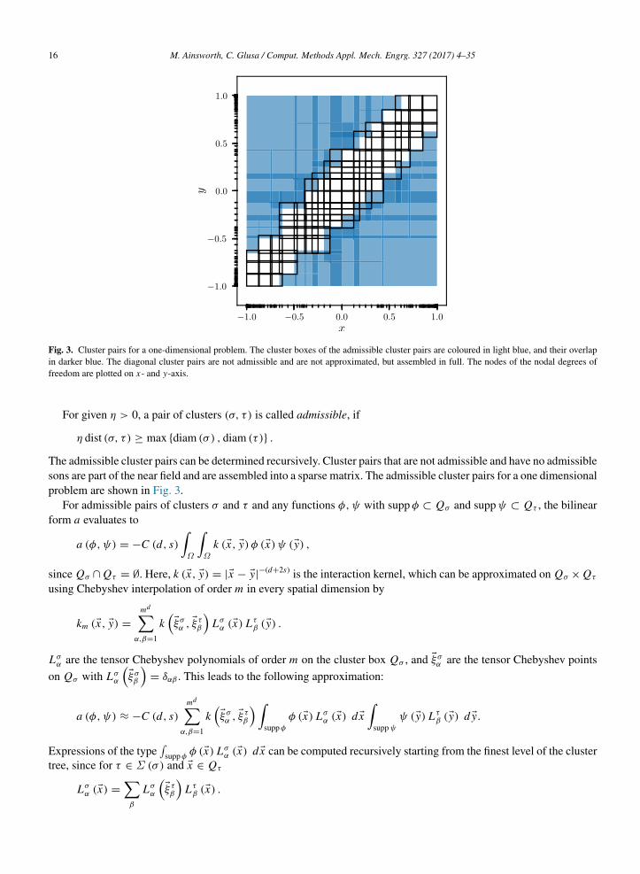
Fig. 3. Cluster pairs for a one-dimensional problem. The cluster boxes of the admissible cluster pairs are coloured in light blue, and their overlapin darker blue. The diagonal cluster pairs are not admissible and are not approximated, but assembled in full. The nodes of the nodal degrees offreedom are plotted on x- and y-axis.

For given η > 0, a pair of clusters (σ, τ ) is called admissible, if

η dist (σ, τ ) ≥ max diam (σ ) , diam (τ ) .

The admissible cluster pairs can be determined recursively. Cluster pairs that are not admissible and have no admissiblesons are part of the near field and are assembled into a sparse matrix. The admissible cluster pairs for a one dimensionalproblem are shown in Fig. 3.

For admissible pairs of clusters σ and τ and any functions φ,ψ with suppφ ⊂ Qσ and suppψ ⊂ Qτ , the bilinearform a evaluates to

a (φ, ψ) = −C (d, s)∫Ω

∫Ω

k (x, y) φ (x) ψ (y) ,

since Qσ ∩ Qτ = ∅. Here, k (x, y) = |x − y|−(d+2s) is the interaction kernel, which can be approximated on Qσ × Qτ

using Chebyshev interpolation of order m in every spatial dimension by

km (x, y) =

md∑α,β=1

k(ξσα , ξ

τβ

)Lσα (x) Lτβ (y) .

Lσα are the tensor Chebyshev polynomials of order m on the cluster box Qσ , and ξσα are the tensor Chebyshev pointson Qσ with Lσα

(ξσβ

)= δαβ . This leads to the following approximation:

a (φ, ψ) ≈ −C (d, s)md∑

α,β=1

k(ξσα , ξ

τβ

) ∫suppφ

φ (x) Lσα (x) dx∫

suppψψ (y) Lτβ (y) d y.

Expressions of the type∫

suppφ φ (x) Lσα (x) dx can be computed recursively starting from the finest level of the clustertree, since for τ ∈ Σ (σ ) and x ∈ Qτ

Lσα (x) =

∑β

Lσα(ξ τβ

)Lτβ (x) .


This means that for all leaves σ = i, and all 1 ≤ α ≤ md , the basis far-field coefficients∫suppφ∩Qσ

φ (x) Lσα (x) dx

need to be evaluated (e.g. by m + 1th order Gaussian quadrature). Moreover, the shift coefficients

Lσα(ξ τβ

)for τ ∈ Σ (σ ) must be computed, as well as the kernel approximations

k(ξσα , ξ

τβ

)for every admissible pair of clusters (σ, τ ). We refer the reader to [32] for further details.

In order for the consistency error of the cluster method to be dominated by the discretization error of the method,the interpolation order m essentially needs to grow with |log hmin|. For further details, we refer to [16,32].

By following the arguments in [32], it can be shown that the number of near field entries scales linearly in n.The same conclusion holds for the number of far field cluster pairs. Since the four dimensional integral contributionsaK×K are evaluated using Gaussian quadrature rules with at most k = O (log n) quadrature nodes per dimension,the assembly of the near field contributions scales with nlog2dn. The far field kernel approximations and the shiftcoefficients have size m2d

= O(log2dn

), and are also calculated in log2dn complexity. This means that all the kernel

approximations and shift coefficients are obtained in nlog2dn time. Finally, the nmd basis far-field coefficients requirethe evaluation of integrals using m + 1th order Gaussian quadrature, leading to a complexity of nlog2dn as well. Theoverall complexity of the cluster method is therefore O

(nlog2dn

), and the sparse approximation requires O

(nlog2dn

)memory. In practice, this means that the assembly of the near-field matrix dominates the other steps but involves onlylocal computations.

The computation of the matrix–vector product involving upward and downward recursion in the cluster tree andmultiplication by the kernel approximations can also be shown to scale with O

(nlog2dn

).

The same principle can be used to evaluate the strong form in all the quadrature nodes necessary for the computationof the BR error indicators. According to Eqs. (20) and (21), a naive implementation scales as O

(n2

). Many of the

components that are used for the cluster method in the matrix–vector product can be reused. Let u =∑

i∈Ihuiφi ∈ Vh ,

and let x0 ∈ K0 be a quadrature node in the evaluation of the local L2-norms in (19). Moreover, let i0 ∈ Ih be theclosest degree of freedom to x0 on K0.

Let (σ, τ ) be an admissible cluster pair such that i0 ∈ σ , and set uτ =∑

j∈τu jφ j , so that supp uτ ⊂ Qτ . Thecontribution to the fractional Laplacian is approximated by

−

∫Qτ

k (x, y) uτ (y) d y = −

∫Qσ

∫Qτ

k (x, y) δ (x − x0) uτ (y) d y d x

≈

md∑α,β=1

k(ξσα , ξ

τβ

) ∫Qσ

Lσα (x) δ (x − x0) dx∫

QτLτβ (y) uτ (y) d y

=

md∑α,β=1

k(ξσα , ξ

τβ

)Lσα (x0)

∫Qτ

Lτβ (y) uτ (y) d y.

The integrals∫

QτLτβ (y) uτ (y) d y already appeared in the computation of the matrix–vector product, and can be

recursively computed. The same holds for the factors Lσα (x0).On the other hand, if the cluster pair (σ, τ ) is not admissible and therefore in the near-field, then formulas Eqs. (20)

and (21) with Ω set to Qσ can be used to evaluate the fractional Laplacian.This shows that the evaluation of the strong form of the fractional Laplacian on all the quadrature nodes

x j

j can be seen as an application of the cluster method with respect to the sets of functionsδ(· − x j

)j

and φi i .


7. Numerical examples

For s ∈ (0, 1), we consider the fractional Poisson problem

(−∆)su = f in Ω = B(0, 1),u = 0 in Ω c

in d ∈ 1, 2 dimensions. Closed-form solutions to the problem posed on a disc are available. In d = 1 dimensions,the solution when the right-hand side is

f 1Dn,0 = 22sΓ (1 + s)2

(s + n − 1/2

s

)(s + n

s

)P (s,−1/2)

n

(2x2

− 1), n ≥ 0

is given by

u1Dn,0 = P (s,−1/2)

n

(2x2

− 1) (

1 − x2)s+,

where(x

y

)=

Γ (x+1)Γ (y+1)Γ (x−y+1) are generalized binomial coefficients, P (α,β)

n are the Jacobi polynomials, and x+ =

max0, x. Moreover, when the right-hand side is given by

f 1Dn,1 = 22sΓ (1 + s)2

(s + n + 1/2

s

)(s + n

s

)x P (s,1/2)

n

(2x2

− 1), n ≥ 0

then the solution is

u1Dn,1 = x P (s,1/2)

n

(2x2

− 1) (

1 − x2)s+

as shown in [25]. Turning to d = 2 dimensions, the solution when the right-hand side is

f 2Dn,ℓ = 22sΓ (1 + s)2

(s + n + ℓ

s

)(s + n

s

)r ℓ cos (ℓθ) P (s,ℓ)

n

(2r2

− 1), ℓ, n ≥ 0

is given by

u2Dn,ℓ = r ℓ cos (ℓθ) P (s,ℓ)

n

(2r2

− 1) (

1 − r2)s+.

For more details on how these analytical solutions are determined, see [25]. Observe that in both the one-dimensionaland the two-dimensional cases, the solutions contain a term which behaves like δ(x)s , where δ (x) is the distance fromx ∈ Ω to the boundary.

7.1. One-dimensional examples

We first solve the fractional Poisson problem with constant right-hand side f = f 1D0,0 and solution u = u1D

0,0 fors = 0.25 and s = 0.75. According to the regularity results in Theorem 1, u is in H s+1/2−ε (Ω), so that we expectessentially h1/2

= O(n−1/2

)convergence if a globally quasi-uniform mesh is used. Using graded meshes, the expected

rate in d = 1 dimensions is ns−2, as shown in Eq. (17).We adaptively refine the mesh based on the BR error indicators and a maximum marking strategy with threshold

0.8. The cluster method is used both for the stiffness matrix and for the evaluation of the strong form of the fractionalLaplacian. The error plots in Fig. 4 clearly display ns−2 convergence in H s-norm, both for s = 0.25 and for s = 0.75,as compared to the n−1/2 convergence obtained by uniform mesh refinement. This means that the optimal rate ofconvergence for d = 1 is achieved. The measured L2-convergence is of order n−1/2−s for uniform refinement and n−2

for adaptive refinement for both values of s.In Fig. 5, we plot the number of degrees of freedom n against timing results for the assembly of the stiffness matrix,

the solution of the linear system, and the computation of the error indicators (19). It can be observed that all threescale with n(log n)2.

Next, we consider the solution of the problem with right-hand side f (x) = sign x ∈ H 1/2−ε (Ω). Based ondecomposition of f with respect to f 1D

n,ℓ , the analytic solution u is found to be

u = 2−2s∑n≥0

(−1)n 2n + s + 3/2n + 1/2

(n+s+1/2−1/2

)(n+s+1/2s

)(n+ss

) x Pn(2x2

− 1) (

1 − x2)s+


Fig. 4. H s - and Ls -error for the one-dimensional problem with constant right-hand side f = f 1D0,0 and for uniform and adaptive refinement.

s = 0.25 at the top, s = 0.75 at the bottom. It can be seen that while uniform refinement results in convergence in H s -norm with rate n−1/2,adaptive refinement achieves the optimal rate of ns−2. The convergence in L2-norm is of order n−1/2−s for uniform refinement, and of order n−2

for adaptive refinement.

so that the discretization error can be calculated as

||u − uh ||2H s (Ω)

= a (u − uh, u − uh) = ( f, u)− ( f, uh) , (30)

with

( f, u) =21−2s

(2s + 1)Γ (1 + s)2

Solutions for s = i/10, i = 1, . . . , 9 are plotted in Fig. 6. For smaller values of s, the transition at the boundaryand at x = 0 is more pronounced, whereas for larger values of s the solutions resemble the solution of the standardinteger-order Poisson problem.

The error plots in Fig. 7 show that ns−2-convergence in H s-norm is also achieved for the discontinuous right-handside f (x) = sign x .


Fig. 5. Timings for assembly of the stiffness matrix, solution of linear system and computation of the error indicators for the one-dimensionalproblem with constant right-hand side f = f 1D

0,0 . s = 0.25 on the left, s = 0.75 on the right. All steps can be seen to scale quasi-linearly with thenumber of unknowns n.

7.2. Two-dimensional examples on the unit disc

We consider the two-dimensional fractional Poisson problem on a disc with constant right-hand side f = f 2D0,0 .

The solutions u for s = 0.25 and s = 0.75 are shown in Fig. 1.Using a globally quasi-uniform mesh, we would obtain h1/2

= O(n−1/4

)convergence. Using a graded mesh,

n−1/2 convergence was predicted, owing to the fact that the mesh is required to be locally quasi-uniform. Again, weadaptively refine the mesh, based on the error indicators (19). The obtained meshes (Fig. 8) are highly refined inregions close to the boundary, where the solution is singular.

We plot the H s (Ω)-error in Fig. 9. It can be observed that n−1/2 convergence is obtained, thus matching the optimalrate obtained using a graded mesh for a constant right-hand side in (18). As in the one-dimensional case, the rate inL2-norm is s orders higher than the rate in H s-norm. By considering the timing results shown in Fig. 10, we see thatall phases of the adaptive refinement loop scale with n(log n)4. The computation of the error indicators is cheaper thanthe assembly of the system matrix, and the solution of the linear system is significantly cheaper than both. Relative to


Fig. 6. Solutions to the one-dimensional fractional Poisson problem with right-hand side f (x) = sign x for s = i/10, i = 1, . . . , 9. For smallervalues of s, the transition at the boundary and at x = 0 is more pronounced, whereas for larger values of s the solutions resemble the solution ofthe standard integer-order Poisson problem.

the matrix assembly, the computation of the error indicators is more expensive than for the one dimensional problem,since it involves numerical quadrature over element edges instead of pointwise evaluations.

We now consider the solution of the problem with right-hand side f (r, θ) = 1|θ |<π/2 ∈ H 1/2−ε (Ω). Based ondecomposition of f with respect to f 2D

n,ℓ , the analytic solution u is found to be

u = 2−2s

(1 − r2

)s+

Γ (1 + s)2

12

+

∑n≥0, ℓ≥1 and odd

(−1)(ℓ+1)/2+n(2n + s + l + 1)π (n + l/2)(s + 1)

cos (ℓθ) r ℓP (s,ℓ)n

(2r2

− 1)(n+s+l/2+1

n+l/2

)(s+nn

)⎫⎬⎭ ,

so that the discretization error can be calculated as

||u − uh ||2H s (Ω)

= a (u − uh, u − uh) = ( f, u)− ( f, uh) ,

with

( f, u) = 2−2s

π

4(s + 1)Γ (s + 1)2

−1π

G3,24,4

(1, 1 + s/2, 5/2 + s, 5/2 + s2, 1/2, 1/2, 2 + s/2

− 1)

,

where G is the Meijer G-function [39].The solutions u for s = 0.25 and s = 0.75 are shown in Fig. 11. The obtained meshes (Fig. 12) are highly refined

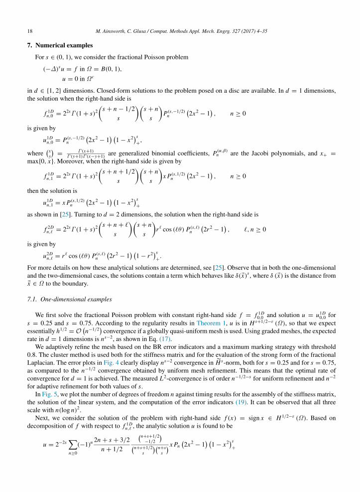
in regions close to the boundary and along the discontinuity θ = ±π/2. We plot the H s-error in Fig. 13, and observethat the optimal rate of convergence of n−1/2 is achieved by adaptive refinement.

7.3. L-shaped domain

We propose to solve the fractional Poisson problem on the L-shaped domain Ω = [0, 2]2\ [1, 2]2 with constant

right-hand side. Since no analytic solution is available, we solve the problem on a highly refined mesh and use thisreference solution uh to approximate the error. In Fig. 16, we show H s- and L2 error, as well as the a posteriorierror estimate η =

(∑i η

2i

)1/2, which is based on the local a posteriori error estimators ηi given in (19). It can be


Fig. 7. H s -error for the one-dimensional problem with discontinuous right-hand side f (x) = sign x and for uniform and adaptive refinement.s = 0.25 at the top, s = 0.75 at the bottom. It can be seen that while uniform refinement results in convergence in H s -norm with rate n−1/2,adaptive refinement achieves the optimal rate of ns−2.

Fig. 8. Adaptively refines meshes for the two-dimensional problem with constant right-hand side. s = 0.25 on the left, s = 0.75 on the right.


Fig. 9. H s - and Ls -error for the two-dimensional problem with constant right-hand side f = f 2D0,0 and for uniform and adaptive refinement.

s = 0.25 at the top, s = 0.75 at the bottom. It can be seen that while uniform refinement results in convergence in H s -norm with rate n−1/4,adaptive refinement achieves the optimal rate of n−1/2. The convergence in L2-norm is of order n−1/4−s/2 for uniform refinement, and of ordern−1/2−s/2 for adaptive refinement.

observed thatuh − uh

H s and the a posteriori error estimate η converge with optimal rate n−1/2, and that

uh − uh

L2

converges with rate n−1/2−s/2. The apparent speed-up of convergence in H s- and L2-norm for larger number ofunknowns is due to the fact that the reference solution uh is used in their computation instead of the true solutionu. The a posteriori error estimate is obviously not suffer this deficiency, because it does not involve the referencesolution uh . This example demonstrates that more complicated domains can easily be considered in the presentedframework, and that convergence of optimal order can equally well be achieved (see Figs. 14 and 15).

7.4. A domain with disconnected components

So far, all the considered domains Ω were simply connected. In fact, this is not a necessary requirement. TakeΩ =

(x, y) ∈ [0, 1]2

| 0.05 ≤ |y − 1/2|

to be a square domain with a strip removed in the middle. Then Ω has twodisconnected components. We take the right-hand side f to be one in the upper part of the domain, and zero in thelower part. Under these conditions, the solution of the regular, integer order Poisson problem is non-zero only on the


Fig. 10. Timings for assembly of the stiffness matrix, solution of linear system and computation of the error indicators for the two-dimensionalproblem with constant right-hand side f = f 2D

0,0 . s = 0.25 on the left, s = 0.75 on the right. All steps can be seen to scale quasi-linearly with thenumber of unknowns n.

Fig. 11. Solutions u corresponding to the discontinuous right-hand side f (r, θ) = 1|θ |<π/2 for s = 0.25 and for s = 0.75.


Fig. 12. Adaptively refined meshes for the discontinuous right-hand side. s = 0.25 on the left, s = 0.75 on the right.

Fig. 13. H s -error for the two-dimensional problem with discontinuous right-hand side f (r, θ) = 1|θ |<π/2 and for uniform and adaptive refinement.s = 0.25 at the top, s = 0.75 at the bottom. Uniform refinement results in convergence in H s -norm with rate n−1/4, adaptive refinement achievesthe optimal rate of n−1/2.


Fig. 14. Solutions u on the L-shaped domain corresponding to a constant right-hand side for s = 0.25 (left) and for s = 0.75 (right).

Fig. 15. Adaptively refined meshes for the L-shaped domain. s = 0.25 on the left, s = 0.75 on the right.

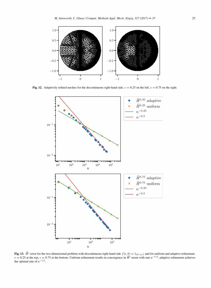
upper part. In the fractional case, however, due to the non-locality of the fractional Laplacian, the solution is positivein the interior of the whole domain, as can be seen in Fig. 17. The corresponding adaptively refined meshes are shownin Fig. 18.

7.5. Exploiting symmetry

The examples of the previous sections displayed symmetries and periodicity in the shape of the domain and theright-hand side and therefore in the solution. In particular, the solution shown in Fig. 11 suggests that one should beable to exploit symmetry to halve the number of degrees of freedom required.

Let B be an orthogonal transformation such that for some K , BK= Id, BΩ = Ω , and let ω ⊂ ω ⊂ Rd be

representative domains such that Rd=

⋃K−1i=0 Bi ω and Ω =

⋃K−1i=0 Biω. Moreover, assume that u

(Bi x

)= u (x)

and f(Bi x

)= f (x). Examples of such transformations for Ω = B(0, 1) include the reflection B = − Id

with ω and ω being the half-space and the half disc, or the rotation by angle θ =2πK and the domains ω =

(r cosφ, r sinφ) ∈ R2| r ≥ 0, φ ∈ [0, 2π/K ]

and ω = ω ∩ r ≤ 1.

The variational formulation of the fractional Poisson problem (3) then reduces to

a (u, v) =C(d, s)

2

∫ω

∫ω

K∑i, j=0

(u

(Bi x

)− u

(B j y

)) (v

(Bi x

)− v

(B j y

))Bi x − B j yd+2s

+ C(d, s)∫ω

∫ω\ω

K∑i, j=0

u(Bi x

)v

(Bi x

)Bi x − B j yd+2s


Fig. 16. H s -, L2-error and estimated error η for the L-shaped domain. s = 0.25 at the top, s = 0.75 at the bottom. Adaptive refinement results inconvergence in H s -norm with optimal rate of n−1/2, and the same holds for the a posteriori error η. In L2-norm, the rate n−1/2−s/2 is observed.

= KC(d, s)

2

∫ω

∫ω

(u (x)− u (y)) (v (x)− v (y)) keff (x, y)

+ K C(d, s)∫ω

∫ω\ω

u (x) v (x) keff (x, y)

and

⟨ f, v⟩ =

K−1∑i=0

∫ω

f(Bi x

)v

(Bi x

)= K

∫ω

f v

with the effective kernel

keff (x, y) =

K−1∑i=0

x − Bi y−d−2s

,


Fig. 17. Solutions u on the two component domain corresponding to a constant right-hand side for s = 0.25 (top) and for s = 0.75 (bottom).

Fig. 18. Adaptively refined meshes for the two component domain. s = 0.25 on the left, s = 0.75 on the right.

that accounts for the interaction with mirror images. Effectively, the computational effort for the assembly and solutionof systems involving the dense stiffness matrix is divided by a factor of K , since only the sub-domain ω needs to bediscretized. The complexity of the cluster method is expected to decrease from O

(n(log n)2d) to O

(n/K (log n)2d)

since the assembly of the near-field contributions constitutes the bulk of the work.To illustrate the approach, we solve the fractional Poisson problem with right-hand side f2,8 on the unit

disc. By leveraging the periodicity in the angular direction (and neglecting the mirror symmetry), we reduce


Fig. 19. Periodic solution u = u2D2,8. Only the circular sector on the right is discretized, with periodic images taken into account through the effective

kernel keff.

to a problem on the circular sector ω =(r cosφ, r sinφ) ∈ R2

| r ≥ 0, φ ∈ [0, π/4]

and ω = ω ∩ r ≤ 1.For simplicity, we employ a uniform mesh and assemble the dense system matrix. The solution is shown inFig. 19.

8. Conclusion

In this work, we have extended the numerical approximation of the fractional Laplacian operator from the caseof globally quasi-uniform meshes to locally refined meshes. In order to overcome slow convergence due to theinherent singularity of the solution close to the boundary, we introduced a posteriori error indicators and adaptivemesh refinement. The non-locality of the problem leads to dense matrices and solution complexity of O

(n3

)using direct solvers and at best O

(n2

)using an optimal iterative method. We showed that by employing a cluster

method, assembly, matrix–vector product and computation of the error estimators scale quasi-linear in the numberof unknowns. This means that the solution of the fractional Poisson problem (1) and the fractional Heat Eq. (2) canbe performed in the same complexity and with equal (or even better) rate of convergence as of the standard integerorder equivalents. Through several one- and two-dimensional examples, we illustrated that the predicted optimal ratesof convergence are obtained. We demonstrated how symmetries and periodicity in the problem can be leveraged toreduce the problem size even further.

Appendix A. Proof of Lemma 4

Lemma 4. For u ∈ Vh and x ∈ K0 for an element K0 ∈ Ph , the fractional Laplacian (−∆)su can be evaluatedas

(−∆)su (x)C (d, s)

=1

d + 2s − 2

∫∂K0

∇u|K0· n y

|x − y|d+2s−2 d y −

u (x)2s

∫∂K0

n y · (x − y)

|x − y|d+2s d y

+

∑K =K0

1

2s(d + 2s − 2)

∫∂K

∇u|K · n y1

|x − y|d+2s−2 d y

−12s

∫∂K

u (y)n y · (x − y)

|x − y|d+2s d y

(20)


if s = 1 − d/2, and as(−∆)su (x)

C (d, s)=

∫∂K0

∇u|K0· n y log

1 x − y d y −

u (x)2s

∫∂K0

n y · (x − y)

|x − y|d+2s d y

+

∑K =K0

12s

∫∂K

∇u|K · n y log1

|x − y|d y

−12s

∫∂K

u (y)n y · (x − y)

|x − y|2 d y

, (21)

when s = 1 − d/2.

Proof. Let u ∈ Vh and x ∈ K0, for some K0 ∈ Ph . Then(−∆)su (x)

C (d, s)= p. v.

∫Rd

u (x)− u (y)

|x − y|d+2s d y

= p. v.∫

K0

u (x)− u (y)

|x − y|d+2s d y + u (x)

∫Rd\K0

1

|x − y|d+2s d y

−

∑K =K0

∫K

u (y)

|x − y|d+2s d y. (A.1)

We have the following helpful identities:

x − y

|x − y|d+2s =

⎧⎪⎪⎨⎪⎪⎩1

d + 2s − 2∇y

1

|x − y|d+2s−2 , s = 1 − d/2,

∇y log1

|x − y|, s = 1 − d/2,

(A.2)

1

|x − y|d+2s =

12s

∇y ·x − y

|x − y|d+2s , (A.3)

1

|x − y|d+2s =

⎧⎪⎪⎨⎪⎪⎩1

2s(d + 2s − 2)∆y

1

|x − y|d+2s−2 , s = 1 − d/2,

1d − 2

∆y log1

|x − y|, s = 1 − d/2.

(A.4)

For x, y ∈ K0,

u (x)− u (y) = ∇u|K0· (x − y)

since u|K0is linear. Hence, the first term of (A.1) can be rewritten using (A.2) as

p. v.∫

K0

u (x)− u (y)

|x − y|d+2s d y = lim

ε→0∇u|K0

·

∫K0\B(x,ε)

x − y

|x − y|d+2s d y

= limε→0

[∇u|K0

·1

d + 2s − 2

∫∂K0

n y

|x − y|d+2s−2 d y

+ ∇u|K0·

1d + 2s − 2

∫∂B(x,ε)

n y

|x − y|d+2s−2 d y

=0

⎤⎥⎥⎥⎦=

1d + 2s − 2

∫∂K0

∇u|K0· n y

|x − y|d+2s−2 d y.

Here, n y is the outward normal at y. When s = 1 − d/2, we obtain instead that

p. v.∫

K0

u (x)− u (y)

|x − y|2 d y =

∫∂K0

∇u|K0· n y log

1 x − y d y.


The second term of (A.1) can be rewritten using (A.3) as∫Rd\K0

1

|x − y|d+2s d y =

12s

∫Rd\K0

∇yx − y

|x − y|d+2s d y

= −12s

∫∂K0

n y · (x − y)

|x − y|d+2s d y.

Finally, for every K ∈ Ph , K = K0, it follows from (A.4), Green’s second identity and (A.2) that∫K

u (y)

|x − y|d+2s d y =

12s(d + 2s − 2)

∫K

u (y)∆y1

|x − y|d+2s−2 d y

=1

2s(d + 2s − 2)

∫K

(∆yu (y)

) =0

1

|x − y|d+2s−2 d y

+1

2s(d + 2s − 2)

∫∂K

u (y) (d + 2s − 2)

n y · (x − y)

|x − y|d+2s

− ∇u|K · n y1

|x − y|d+2s−2

d y

=12s

∫∂K

u (y)n y · (x − y)

|x − y|d+2s d y −

12s(d + 2s − 2)

∫∂K

∇u|K · n y1

|x − y|d+2s−2 d y.

When s = 1 − d/2, we obtain instead that∫K

u (y)

|x − y|d+2s d y =

12s

∫∂K

u (y)n y · (x − y)

|x − y|2 d y −

12s

∫∂K

∇u|K · n y log1

|x − y|d y.

In conclusion, we find that

(−∆)su (x)C (d, s)

=1

d + 2s − 2

∫∂K0

∇u|K0· n y

|x − y|d+2s−2 d y −

u (x)2s

∫∂K0

n y · (x − y)

|x − y|d+2s d y

+

∑K =K0

1

2s(d + 2s − 2)

∫∂K

∇u|K · n y1

|x − y|d+2s−2 d y −

12s

∫∂K

u (y)n y · (x − y)

|x − y|d+2s d y

and when s = 1 − d/2 then

(−∆)su (x)C (d, s)

=

∫∂K0

∇u|K0· n y log

1 x − y d y −

u (x)2s

∫∂K0

n y · (x − y)

|x − y|d+2s d y

+

∑K =K0

12s

∫∂K

∇u|K · n y log1

|x − y|d y −

12s

∫∂K

u (y)n y · (x − y)

|x − y|2 d y

.

Appendix B. Determination of quadrature orders

Theorem 9 ([32], Theorems 5.3.23 and 5.3.24). If K and K (K and e) are touching elements, thenE i, jK×K

≤ Ch2−2sK ρ

−2kT1 ,E i, j

K×e

≤ Ch2−2sK ρ

−2kT,∂3 ,

where ρ1, ρ3 > 1 and kT , kT,∂ are the quadrature orders in every dimension of Eqs. (23) and (24) (afterregularization).

If K and K (K and e) are not touching, thenE i, jK×K

≤ C(hK h K

)2d−2−2sK ,K

(dK ,K

hK

)2

ρ2

(K , K

)−2kN T+

(dK ,K

h K

)2

ρ2

(K , K

)−2kN T

,

32 M. Ainsworth, C. Glusa / Comput. Methods Appl. Mech. Engrg. 327 (2017) 4–35E i, jK×e

≤ C(hK he)2d−2−2s

K ,e

(dK ,e

hK

)2

ρ4(K , e)−2kN T +

(dK ,e

he

)2

ρ4(e, K )−2kN T

,

where dK ,K := dist(K , K ), dK ,e := dist(K , e), ρ2(K , K ) := ρ2 max dK ,K

hK, 1

, ρ4(K , e) := ρ4 max

dK ,ehK, 1

and

ρ2, ρ4 > 1, and kN T , kN T,∂ are the quadrature order in every dimension of Eqs. (23) and (24).

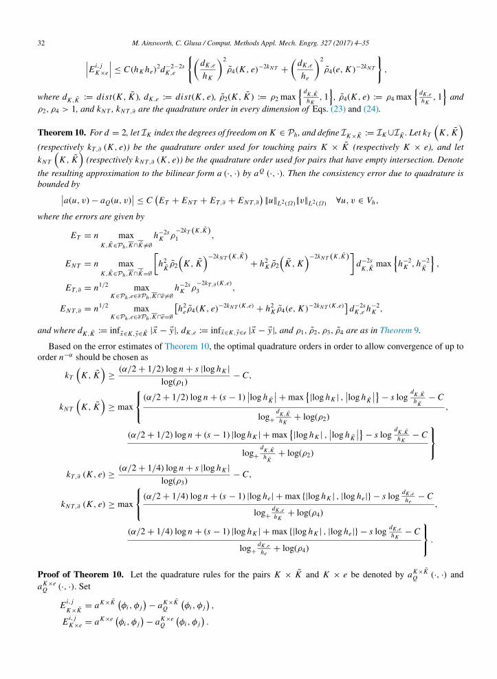
Theorem 10. For d = 2, let IK index the degrees of freedom on K ∈ Ph , and define IK×K := IK ∪IK . Let kT

(K , K

)(respectively kT,∂ (K , e)) be the quadrature order used for touching pairs K × K (respectively K × e), and letkN T

(K , K

)(respectively kN T,∂ (K , e)) be the quadrature order used for pairs that have empty intersection. Denote

the resulting approximation to the bilinear form a (·, ·) by aQ (·, ·). Then the consistency error due to quadrature isbounded bya(u, v) − aQ(u, v)

≤ C(ET + EN T + ET,∂ + EN T,∂

)||u||L2(Ω)||v||L2(Ω) ∀u, v ∈ Vh,

where the errors are given by

ET = n maxK ,K∈Ph ,K∩K =∅

h−2sK ρ

−2kT (K ,K)1 ,

EN T = n maxK ,K∈Ph ,K∩K=∅

[h2

Kρ2

(K , K

)−2kN T (K ,K)+ h2

K ρ2

(K , K

)−2kN T (K ,K)]

d−2sK ,K

max

h−2K , h−2

K

,

ET,∂ = n1/2 maxK∈Ph ,e∈∂Ph ,K∩e =∅

h−2sK ρ

−2kT,∂ (K ,e)3 ,

EN T,∂ = n1/2 maxK∈Ph ,e∈∂Ph ,K∩e=∅

[h2

e ρ4(K , e)−2kN T (K ,e) + h2K ρ4(e, K )−2kN T (K ,e)

]d−2s

K ,e h−2K ,

and where dK ,K := infx∈K ,y∈K |x − y|, dK ,e := infx∈K ,y∈e |x − y|, and ρ1, ρ2, ρ3, ρ4 are as in Theorem 9.

Based on the error estimates of Theorem 10, the optimal quadrature orders in order to allow convergence of up toorder n−α should be chosen as

kT

(K , K

)≥(α/2 + 1/2) log n + s |log hK |

log(ρ1)− C,

kN T

(K , K

)≥ max

⎧⎨⎩ (α/2 + 1/2) log n + (s − 1)log h K

+ max|log hK | ,

log h K

− s logdK ,Kh K

− C

log+

dK ,KhK

+ log(ρ2),

(α/2 + 1/2) log n + (s − 1) |log hK | + max|log hK | ,

log h K

− s logdK ,KhK

− C

log+

dK ,Kh K

+ log(ρ2)

⎫⎬⎭kT,∂ (K , e) ≥

(α/2 + 1/4) log n + s |log hK |

log(ρ3)− C,

kN T,∂ (K , e) ≥ max

⎧⎨⎩ (α/2 + 1/4) log n + (s − 1) |log he| + max |log hK | , |log he| − s log dK ,ehe

− C

log+

dK ,ehK

+ log(ρ4),

(α/2 + 1/4) log n + (s − 1) |log hK | + max |log hK | , |log he| − s log dK ,ehK

− C

log+

dK ,ehe

+ log(ρ4)

⎫⎬⎭ .Proof of Theorem 10. Let the quadrature rules for the pairs K × K and K × e be denoted by aK×K

Q (·, ·) andaK×e

Q (·, ·). Set

E i, jK×K

= aK×K (φi , φ j

)− aK×K

Q

(φi , φ j

),

E i, jK×e = aK×e (

φi , φ j)− aK×e

Q

(φi , φ j

).


For u, v ∈ Vh , we set

EK×K (u, v) =

∑i∈IK×K

∑j∈IK×K

uiv j E i, jK×K

,

EK×e(u, v) =

∑i∈IK

∑j∈IK

uiv j E i, jK×e

so thatEK×K (u, v) ≤

(max

i, j

E i, jK×K

) ∑i∈IK×K

|ui |∑

j∈IK×K

v j

≤

(max

i, j

E i, jK×K

) IK×K

√ ∑i∈IK×K

|ui |2√ ∑

j∈IK×K

v j2,

|EK×e(u, v)| ≤

(max

i, j

E i, jK ,e

) ∑i∈IK

|ui |∑j∈IK

v j

≤

(max

i, j

E i, jK ,e

) |IK |

√∑i∈IK

|ui |2√ ∑

j∈IK

v j2

Since ∑i∈IK×K

|ui |2

≤ C[

h−dK

∫K

u2+ h−d

K

∫K

u2],

∑i∈IK

|ui |2

≤ Ch−dK

∫K

u2,

we finda(u, v) − aQ(u, v) ≤

∑K

∑K

EK×K (u, v) +

∑K

∑e

|EK×e(u, v)|

≤ C∑

K

∑K

(max

i, j

E i, jK×K

) max

h−dK , h−d

K

[||u||

2L2(K ) + ||u||

2L2(K )

]1/2

[||v||2L2(K ) + ||v||2

L2(K )

]1/2

+ C∑

K

∑e

(max

i, j

E i, jK×e

) h−dK ||u||L2(K )||v||L2(K )

≤ C(

maxK ,K

maxi, j

E i, jK×K

max

h−dK , h−d

K

) ∑K

∑K

||u||L2(K∪K )||v||L2(K∪K )

+ C(

maxK ,e

maxi, j

E i, jK×e

h−dK

) ∑K

∑e

||u||L2(K )||v||L2(K ).

Because∑K

∑K

||u||L2(K∪K )||v||L2(K∪K ) ≤

√∑K

∑K

||u||2L2(K∪K )

√∑K

∑K

||v||2L2(K∪K )

≤ 2 |Ph | ||u||L2(Ω)||v||L2(Ω)

≤ Cn||u||L2(Ω)||v||L2(Ω)


and ∑K

∑e

||u||L2(K )||v||L2(K ) ≤ |∂Ph | ||u||L2(Ω)||v||L2(Ω)

≤ Cn(d−1)/d||u||L2(Ω)||v||L2(Ω),

we obtaina(u, v) − aQ(u, v) ≤ C

[n

(maxK ,K

maxi, j

E i, jK×K

max

h−dK , h−d

K

)+ n(d−1)/d

(maxK ,e

maxi, j

E i, jK×e

h−dK

)]||u||L2(Ω)||v||L2(Ω).

For d = 2, using Theorem 9 stated below permits to conclude.

References

[1] J.T. Oden, T. Sato, Finite strains and displacements of elastic membranes by the finite element method, Int. J. Solids Struct. 3 (4) (1967)471–488.

[2] J.T. Oden, Analysis of large deformations of elastic membranes by the finite element method, in: Proc. IASS Int. Congress of Large-SpanShells, 1966, Leningrad.

[3] J.T. Oden, W. Kubitza, Numerical Analysis of Nonlinear Pneumatic Structures, Clearinghouse, 1967.[4] J.T. Oden, Finite element analysis of nonlinear problems in the dynamical theory of coupled thermoelasticity, Nucl. Eng. Des. 10 (4) (1969)

465–475.[5] J.T. Oden, Finite-element analogue of Navier-Stokes equation, J. Eng. Mech. Div. 96 (4) (1970) 529–534.[6] J.T. Oden, J. Key, Numerical analysis of finite axisymmetric deformations of incompressible elastic solids of revolution, Int. J. Solids Struct.

6 (5) (1970) 497–518.[7] L. Demkowicz, J.T. Oden, W. Rachowicz, O. Hardy, Toward a universal hp adaptive finite element strategy, Part 1. Constrained approximation

and data structure, Comput. Methods Appl. Mech. Engrg. 77 (1–2) (1989) 79–112.[8] J.T. Oden, L. Demkowicz, W. Rachowicz, T. Westermann, Toward a universal hp adaptive finite element strategy, Part 2. A posteriori error

estimation, Comput. Methods Appl. Mech. Engrg. 77 (1–2) (1989) 113–180.[9] M. Ainsworth, J.T. Oden, A Posteriori Error Estimation in Finite Element Analysis, Vol. 37, John Wiley & Sons, 2011.

[10] A. Toselli, O. Widlund, Domain Decomposition Methods: Algorithms and Theory, Vol. 3, Springer, 2005.[11] B.J. West, Fractional Calculus View of Complexity: Tomorrow’s Science, CRC Press, 2016.[12] M.M. Meerschaert, A. Sikorskii, Stochastic models for fractional calculus, in: de Gruyter Studies in Mathematics, vol. 43, Walter de Gruyter

& Co., Berlin, 2012, p. x+291.[13] R.H. Nochetto, E. Otárola, A.J. Salgado, A PDE approach to fractional diffusion in general domains: a priori error analysis, Found. Comput.

Math. 15 (3) (2015) 733–791.[14] R. Servadei, E. Valdinoci, On the spectrum of two different fractional operators, Proc. Roy. Soc. Edinburgh Sect. A 144 (04) (2014) 831–855.[15] G. Acosta, J.P. Borthagaray, A fractional Laplace equation: regularity of solutions and Finite element approximations, 2015. ArXiv e-prints

arXiv:1507.08970.[16] M. Ainsworth, C. Glusa, Towards an efficient finite element method for the integral fractional laplacian on polygonal domains, TBD (2017).[17] W.C.H. McLean, Strongly Elliptic Systems and Boundary Integral Equations, Cambridge University Press, 2000.[18] K. Bogdan, K. Burdzy, Z.-Q. Chen, Censored stable processes, Probab. Theory Related Fields 127 (1) (2003) 89–152.[19] Z.-Q. Chen, P. Kim, Green function estimate for censored stable processes, Probab. Theory Related Fields 124 (4) (2002) 595–610.[20] M. D’Elia, M. Gunzburger, The fractional Laplacian operator on bounded domains as a special case of the nonlocal diffusion operator,

Comput. Math. Appl. 66 (7) (2013) 1245–1260.[21] G. Grubb, Fractional laplacians on domains, a development of Hörmander’s theory ofµ-transmission pseudodifferential operators, Adv. Math.

268 (2015) 478–528.[22] G. Acosta, F.M. Bersetche, J.-P. Borthagaray, A short FE implementation for a 2d homogeneous Dirichlet problem of a fractional Laplacian,

2016. ArXiv e-prints arXiv:1610.05558.[23] A. Ern, J.-L. Guermond, Theory and Practice of Finite Elements. Applied Mathematical Sciences, Vol. 159, Springer, New York, NY, 2004.[24] R.K. Getoor, First passage times for symmetric stable processes in space, Trans. Amer. Math. Soc. 101 (1) (1961) 75–90.[25] B. Dyda, A. Kuznetsov, M. Kwasnicki, Fractional Laplace operator and Meijer g-function, Constr. Approx. (2016) 1–22.[26] L.R. Scott, S. Zhang, Finite element interpolation of nonsmooth functions satisfying boundary conditions, Math. Comp. 54 (190) (1990)

483–493.[27] P. Ciarlet, Analysis of the Scott–Zhang interpolation in the fractional order Sobolev spaces, J. Numer. Math. 21 (3) (2013) 173–180.[28] M. Ainsworth, W. McLean, T. Tran, The conditioning of boundary element equations on locally refined meshes and preconditioning by

diagonal scaling, SIAM J. Numer. Anal. 36 (6) (1999) 1901–1932.[29] S.C. Brenner, L. Scott, The Mathematical Theory of Finite Element Methods, second ed., Springer, Berlin, 2002.

http://refhub.elsevier.com/S0045-7825(17)30599-6/sb1



























http://arxiv.org/abs/1507.08970






















































[30] B. Faermann, Localization of the Aronszajn-Slobodeckij norm and application to adaptive boundary elements methods. Part I. The two-dimensional case, IMA J. Numer. Anal. 20 (2) (2000) 203–234.

[31] B. Faermann, Localization of the Aronszajn-Slobodeckij norm and application to adaptive boundary element methods Part II. The three-dimensional case, Numer. Math. 92 (3) (2002) 467–499.

[32] S.A. Sauter, C. Schwab, Boundary Element Methods, Springer, 2010, pp. 183–287.[33] A. Chernov, T. von Petersdorff, C. Schwab, Exponential convergence of hp quadrature for integral operators with Gevrey kernels, ESAIM

Math. Model. Numer. Anal. 45 (3) (2011) 387–422.[34] A. Chernov, C. Schwab, Exponential convergence of Gauss–Jacobi quadratures for singular integrals over simplices in arbitrary dimension,

SIAM J. Numer. Anal. 50 (3) (2012) 1433–1455.[35] A. Chernov, T. von Petersdorff, C. Schwab, Quadrature algorithms for high dimensional singular integrands on simplices, Numer. Algorithms

70 (4) (2015) 847–874.[36] W. Hackbusch, Multi-Grid Methods and Applications, Vol. 4, Springer-Verlag, Berlin, 1985.[37] W. Hackbusch, Iterative solution of large sparse systems of equations, in: Applied Mathematical Sciences, vol. 95, Springer-Verlag, New

York, 1994, p. xxii+429.[38] M. Ainsworth, W. McLean, Multilevel diagonal scaling preconditioners for boundary element equations on locally refined meshes, Numer.

Math. 93 (3) (2003) 387–413.[39] E.W. Weisstein, Meijer G-Function. From MathWorld—A Wolfram Web Resource. Last visited on 2/23/2017, 2017. URL http://mathworld.

wolfram.com/MeijerG-Function.html.
























http://mathworld.wolfram.com/MeijerG-Function.html


















































aspects of an adaptive finite element method for the ... · pointwise integer-order derivatives are...

Documents