asiaphoria meets regression to the mean · asiaphoria meets regression to the mean ... rates over...
TRANSCRIPT

33
Asiaphoria Meets Regression to the MeanLant Pritchett and Lawrence Summers
Consensus forecasts for the global economy over the medium and long term call for a substantial shift of economic gravity towards Asia and especially towards the Asian giants, China and India. While such forecasts may pan out, there are substantial reasons to expect that growth in China and India will be much less rapid than is currently anticipated. Most importantly history teaches that while economic forecasts invariably extrapolate recent growth, abnormally rapid growth is rarely persistent. Indeed regression to the mean is the empirically most salient feature of economic growth, showing far more robustness in the data than, say, the much-discussed middle-income trap. Furthermore, statistical analysis of growth reveals that in developing countries, episodes of rapid growth are frequently punctuated by discontinuous drop-offs in growth. Such discontinuities account for a large fraction of the variation in growth rates. We suggest that salient characteristics of China—high levels of state control and corruption along with low measures of authoritarian rule—make a discontinuous decline in growth even more likely than general experience would suggest. China’s growth record in the past 35 years has been remarkable, and nothing in our analysis suggests that a sharp slowdown is inevitable. Still, our analysis suggests that forecasters and planners looking at China would do well to contemplate a much wider range of outcomes than is typically considered.
1. introductionThe rise of Asia is a story in at least four parts, with the fourth yet to be writ-ten. The first is the dramatic rise of Japan before and after World War II, ulti-mately to a prosperous and productive economy and global leader by the late 1980s. The second is the rise beginning in the 1960s of the East Asian Drag-ons—led by the four “Asian Tigers” of Korea, Taiwan, Singapore, and Hong Kong and followed by the three larger economies of Southeast Asia, Malaysia, Indonesia, and Thailand. The third is the rise of the Asian giants with popula-tions of over one billion. China and India each have more than twice the popula-tion of the other eight East Asian economies combined.
authors’note: We would like to thank David Yang for his able assistance and discussants ChangTai Hseih and Robert Feenstra and participants at the 2013 Asian Economic Policy Conference for helpful comments and insights.

34 ASIA EC ONOMIC P OLICY C ONFERENCE PROSPEC T S FOR ASIA AND THE GLOBAL EC ONOM Y
At least since the 1980s, economic growth accelerated in both China and India and then, surprisingly given usual historical patterns, accelerated again in both countries in the 1990s. That was followed by another acceleration in India in the mid-2000s (Kar et al. 2013). The power of compound interest over long periods at high rates plus their sheer scale in population have led both economies to become global economic powerhouses. In purchasing power par-ity data (PPP) from the Penn World Tables (PWT) 8.0 (Feenstra, Inklar and Timmer 2013), the three largest economies in the world in 2011 are the United States, China, and India. China’s economy is now, again at PPP, roughly three times Japan’s and four times Germany’s.1
The fourth stage of this Asian story, the future, is unknown. Extrapolat-ing a decade or two into the future—based on recent growth rate differentials between China and India, the modest post-crisis growth of the United States, and the even more modest recent growth in Europe—produces an Asiaphoria, the view that the global economy will increasingly be shaped and lifted by the trajectory of the giants. Combined with continued growth in the other large Asian economies that still have low to middle incomes—for example, Vietnam, Indonesia, and Thailand—the vision of the global economic center of gravity shifting even more decisively to Asia becomes destiny.
Asiaphoria has become almost conventional wisdom. Looking to 2060: LongTerm Global Growth Prospects (OECD 2012) forecasts per capita growth from 2011 to 2030 for China of 6.6 percent and for India, 6.7 percent. In China 2030 the World Bank (2012) and the Development Research Center of the State Council of China project output per worker growth rates of 8.3 percent from 2011 to 2015, 7.1 percent from 2016 to 2020, and 6.2 percent from 2021 to 2025. In its official National Intelligence Estimates projected out to 2030, the U.S. intelligence community presents scenarios implying China’s share of the world economy will grow from 6.4 percent in 2010 to between 17 and 23 percent in 2030; for India the estimates for the same periods are growth building from 1.8 percent of the world economy to between 6.5 and 7.9 percent. And these are cautious contrasted with Fogel’s (2010) prediction that China’s GDP will reach US$123 trillion by 2040.
Our principle contribution is a rigorous quantitative demonstration that with respect to economic growth—just as investment firms warn is true about returns—past performance is no guarantee of future performance. Regression to the mean is perhaps the single most robust and empirical relevant fact about cross-national growth rates. The lack of persistence in country growth rates over medium- to long-run horizons implies current growth has very lit-tle predictive power for future growth. Hence, while it might be the case that

PRITCHE T T & SUMMERS | ASIAPHORIA MEE T S REGRES SION TO THE ME AN 35
China will continue for another two decades at 9 (or even 7 or 6) percent per capita growth, given the regression to the mean present in the cross-national data, where historically the distribution of growth has been an average of 2 per-cent with a standard deviation of 2 percent, this would be an extraordinary tail event. Similarly, while it might be the case that Indian growth continues at 6 percent, this would require India’s extended growth, already rare, to persist even longer and become rarer still.
Many of the great economic forecasting errors of the past half-century came from excessive extrapolation of performance in the recent past and treat-ing a country’s growth rate as a permanent characteristic rather than a tran-sient condition. Paul Samuelson’s textbook predicted in 1961 that there was a substantial chance that the USSR would overtake the United States economi-cally by the 1980s. There was a widespread view right up until the end of the 1980s that Japan would continue to outcompete the world. Or in the opposite direction, consider the pervasive pessimism of a decade ago regarding Africa. Since then, African countries emerged as a majority of the world’s most rapidly growing nations.
In addition to demonstrating that past growth performance is of very little value for forecasting the central tendency of future growth, we also show that in developing countries the growth process is marked by sharp discontinuities, with very large accelerations or decelerations of growth being quite common. This implies that the explicit (or implicit) confidence intervals in typical fore-casts or the range of growth that scenarios consider might dramatically under-estimate the actual range of outcomes. The recent crisis has again alerted us to the fact that risks of downside scenarios are often vastly underestimated,2 just as the fragility in systems is underestimated. Moreover it appears that particu-lar aspects of China’s situation—a high degree of government discretion vis-à-vis businesses and an authoritarian regime—add to the likelihood of a growth slowdown.
Our paper is organized as follows. Section 1 presents the basic evidence on regression to the mean in country growth rates and shows how taking account of this evidence leads to forecasts for Chinese and Indian growth that are much more pessimistic than consensus views. Section 2 demonstrates the robustness of the conclusion to a variety of specifications. Section 3 draws on recent work by Kar et al. (2013) that extends work on “stop-start” growth (e.g., Rodrik 1999 and Jones and Olken 2008) and shows the extent to which the growth process is marked by changes in “growth regimes” with large accelerations and decelera-tions. This is a very different view than the standard trend-cycle model used in industrial country macroeconomics, but it appears to be much more descriptive

36 ASIA EC ONOMIC P OLICY C ONFERENCE PROSPEC T S FOR ASIA AND THE GLOBAL EC ONOM Y
of developing countries where “the cycle is the trend” (Aguiar and Gopinath 2007). We show that rapidly growing countries are substantially more likely to suffer a downward discontinuity in growth than an upward movement. Our analysis also suggests that growth declines are more likely to be sudden and large than gradual and small. Section 3 also demonstrates that, in consider-ing China’s prospects for continued rapid growth, the much-discussed middle income trap is less a fundamental empirical issue than a simple regression to the mean (if, properly measured, it even exists). Finally, Section 4 considers two qualitative aspects of the Chinese situation—China’s high degree of depen-dence on discretionary policies towards business and its authoritarian char-acter. We show that both make sharp declines in growth more likely. A final section concludes and discusses some implications of the results.
2. The $42 Trillion Question: Will Rapid growth in China and india persist?
2.1. Regression to the Mean: The Single Most Robust Fact about Growth
The 1990s saw an explosion of “growth regressions” which placed the growth of gross domestic product per capita (GDPPC) over some period on the left-hand side and everything but the kitchen sink on the right (Wacziarg 2002 and Rodri-guez and Shelton 2013).3 We are not going to characterize what was “learned,” as the methodological sensitivity of growth regression findings about particular variables was an issue raised early (Levine and Renelt 1992) and often: Nearly every assertion about correlates (or causes) of growth emerging in any study has been challenged as not robust in a later study.
However, one fact about growth that emerged early—including a paper of ours with Bill Easterly and Michael Kremer (Easterly et al. 1993)—has stood the test of time and new data: There is strong regression to the mean in the growth process, hence very little persistence in country growth rate differ-ences over time, and consequently current growth has a low predictive power for future growth. Although one might have thought that most of the long hori-zon growth differences were due to the existence of fast and slow growing coun-tries (e.g., Argentina grows slow and Japan grows fast)—the opposite is true and nearly all growth variation is due to differences within countries over time.
Table 1 presents four measures of persistence: the correlation, the rank cor-relation (to reduce the influence of outliers), the regression coefficient of cur-rent growth on lagged growth, and the R-squared of the regression (which is of course the square of the correlation coefficient). We use the PWT8.0 (Feen-stra, Inklar, and Timmer 2013) data on local currency real GDP from national

PRITCHE T T & SUMMERS | ASIAPHORIA MEE T S REGRES SION TO THE ME AN 37
accounts (since we are not yet comparing levels) and population to compute real GDPPC. We compute least-squares growth rates of natural log GDPPC for 10 and 20 year periods for all countries with sufficient data.4 The results show that the low persistence of growth has been a consistent and robust characteristic across all decades—if anything there is less persistence in the recent decadal growth rates (1990–2000 to 2000–10) than in previous decades.5 Not surpris-ingly, the persistence declines over longer periods so that using current growth rates to predict two decades ahead has even less predictive power than predict-ing one decade ahead.
The results in Table 2 using growth rates over 20 year periods—which smooth even more over “cyclical” fluctuations—are similar in showing strong regression to the mean, low persistence, and low predictive power of current growth for future growth.
For the question at hand—Will the rapid growth rates of the Asian giants continue into coming decades as an engine of global growth?—the most relevant summary statistics are the regressions.
First, knowing the current growth rate only modestly improves the pre-diction of future growth rates over just guessing it will be the (future realized) world average. The R-squared of decade-ahead predictions of decade growth varies from 0.056 (for the most recent decade) to 0.13. Past growth is just not that informative about future growth and its predictive ability is generally even lower over longer horizons.
TA b l e 1
little persistence in Cross-national growth Rates across Decades
Period1 Period2 Correlation Rank Regression R-squared N Correlation Coefficient
Adjacent decades1950–60 1960–70 0.363 0.381 0.378 0.132 661960–70 1970–80 0.339 0.342 0.382 0.115 1081970–80 1980–90 0.337 0.321 0.323 0.114 1421980–90 1990–2000 0.361 0.413 0.288 0.130 1421990–2000 2000–10 0.237 0.289 0.205 0.056 142One decade apart1950–60 1970–80 0.079 0.192 0.095 0.006 661960–70 1980–90 0.279 0.312 0.306 0.078 1081970–80 1990–2000 0.214 0.214 0.163 0.046 1421980–90 2000–10 0.206 0.137 0.143 0.043 142Two decades apart1960–70 1990–2000 0.152 0.177 0.152 0.023 1081970–80 2000–10 –0.022 0.005 –0.015 0.001 142Source: Author’s calculations with Penn World Tables (PWT8.0) data (Feenstra, Inklaar, and Timmer 2013).

38 ASIA EC ONOMIC P OLICY C ONFERENCE PROSPEC T S FOR ASIA AND THE GLOBAL EC ONOM Y
Second, if all we knew was a country’s current growth rate then what would be the best prediction of the future? The extremes are extrapolation, a coef-ficient of 1, and exclusion, a coefficient of zero. Our estimates imply that the coefficients are around 0.3 for decade-ahead predictions and lower if current decades are used to predict further ahead, 0.2 or less.
Essentially what is being asserted here is the equivalent of the Time mag-azine cover curse. It has been observed that public figures who appear on the cover of Time often suffer a career reversal soon afterwards. This is just what one would expect with mean reversion and extrapolative expectations. Those who perform best in period t will on average perform much worse than expected in period t 1+ .
At a deeper level, the finding of high mean reversion in growth rates has profound implications for the study of economic growth. If it were the case as many models suggest that some relatively constant feature of countries—their climate, their culture, the quality of their institutions, or their openness to the world as examples—influenced growth, importantly one would expect since these variables persist that growth rates would persist. That growth rates do not persist suggests that factors of this kind should be analyzed as affecting the level but not the long-run growth of incomes. This suggests that, unless a country can either continually improve its policy environment or its governance, even the most favorable conditions will ultimately have diminishing impacts on growth.
2.2. Forecasting the Future level of GDP in the Giants
What are the mechanical implications for the predicted growth of dollar GDP of China and India of “extrapolation of current growth” versus regression to the mean? By “mechanical” we just mean, what we would expect to happen if we did not know anything about China or India and just treated them as if they would follow the statistical regularities that apply to other countries?
TA b l e 2
Twenty-Year periods show modest persistence; Hence Current growth Has little Value for predicting Future growth
Period1 Period2 Correlation Rankcorrelation Regressioncoefficient R-squared N
Adjacent two decade periods1950–70 1970–90 0.258 0.318 0.343 0.067 701960–80 1980–2000 0.459 0.454 0.494 0.211 1081970–90 1990–2010 0.327 0.325 0.215 0.107 142Gap of two decades1950–70 1990–2010 0.047 0.015 0.047 0.002 70Source: Authors’ calculations with PWT8.0 data (Feenstra, Inklaar, and Timmer 2013).

PRITCHE T T & SUMMERS | ASIAPHORIA MEE T S REGRES SION TO THE ME AN 39
We create predictions of growth rates in future decades using regressions that predict countries’ growth rates based on their past decades’ growth (and their initial levels of income in PPP to allow for convergence). Predictions then just plug China’s and India’s current growth rates and levels of income into that equation and roll these predictions forward for two decades. The basic idea (on which we experiment with many variants) is to estimate equation (1):
(1) 10 00 ln( )g g y00 90 00i i i i) )a b c f= + + +- - ,
and then predict growth ahead for two decades using the estimated coefficients and the actual values for China and India for the first decade and the predicted growth (and consequent level) for the first decade in predicting the second:
10 ln( )gp g y13 23 00 2010China China China) )a b c= + +- -t t t
ln( )gp gp yp23 33 13 33 2023China China China) )a b c= + +- -t t t .
Table 3 shows the results of a variety of simple “regression to the mean” regressions, with and without convergence terms, with and without two decades of lags, and for 10 versus 20 year time periods. Not surprisingly given the robust-ness of weak persistence as a feature of growth rates demonstrated above, all regressions produce coefficients on lagged growth between 0.20 and 0.32.
Because our primary interest is the impact on the global economy, we pre-dict total GDP in dollars (not PPP adjusted) for China and India over the next two decades.6 To predict population we use the United Nations Medium Fertil-ity projections, which show China’s population growth near zero while India’s continues to grow about 1 percent per year over the next decade and then slows.
We start the scenarios using the International Monetary Fund (IMF) World Economic Outlook 2013 U.S. dollar GDP (which is somewhat a forecast, but, for instance, already includes the depreciation of the rupee in 2013). We compute total dollar GDP for 2023 and 2033 by simply using an assumed growth rate of GDP per capita and then multiplying by population.
The results are at the same time obvious and striking. If one assumes a con-tinuation of current growth rates, the 20 year gain in GDP from 2013 to 2033 in China would be $51.1 trillion (from $8.9 to $60 trillion), which would be a gain in GDP more than three times as large as the current U.S. economy. The continu-ation of current growth rates would make China far and away the world’s dom-inant economy. The gain in India would be smaller (as it begins from a lower base and at a lower growth rate, of 6 percent) but still rises to a substantial $6.8 trillion for a gain of $5.1 trillion (the current size of France and Italy combined).

40 ASIA EC ONOMIC P OLICY C ONFERENCE PROSPEC T S FOR ASIA AND THE GLOBAL EC ONOM Y
Even if one assumes growth slows in China to 7 percent its total GDP grows to $36 trillion—more than twice the current U.S. level.
However, it is also obvious that regression to the mean of the ordinary type would reduce these gains massively. Under any of the empirical estimates for “regression to the mean,” the level of China’s GDP in 2033 would fall to around $20 trillion—which still implies a 20 year increase in GDP of around $11 trillion. Similarly, the gains in India fall from $5 trillion to between $2.4 and $3.3 tril-lion. It is noteworthy that the forecasts based on past growth and levels predict growth that is closer to the naive expectation that China and India will grow like average countries than to extrapolations of their past growth.
There is some consensus that China will not maintain 9 to 10 percent growth rates, but even the view that China’s growth will slow to something like 7 per-cent assumes substantial persistence (Table 4). The predicted growth over the next two decades using regressions is 3.89 percent (with a coefficient on past growth of 0.24), and the regression standard error of estimation is 1.6 percent, so a continuation of even 7 percent is two standard deviations in the tail, and a continuation of a growth rate of 9 percent is three standard deviations.
Table 5 shows that whether or not China and India will maintain their cur-rent growth or be subject to regression to the global mean growth rate is a 42 trillion dollar question. The difference between the “continuation” scenario in 2033, in which the GDP of China plus India gains $56 trillion, and the average of the “regression to the mean” scenarios (which are all quite similar, with total China plus India 2033 GDP between $12 and $15.5 trillion) is $42 trillion dol-lars. The 7 percent scenario shows a gain of $33 trillion versus $13 trillion of the average of the regression to the mean scenarios.
TA b l e 3
Regressions of Decade growth Rates on past Decade growth Rates, allowing for lagged level of income
Dependentvariable Constant Lagged Secondlag InitialLevel R2 N growth ofgrowth ofGDPPC
Growth 2000–10 Coefficient 0.023 0.205 0.056 142 t-stat 10.758 2.887 Growth 2000–10 Coefficient 0.068 0.329 –0.006 0.177 142 t-stat 6.632 4.572 –4.519 Growth 2000–10 Coefficient 0.074 0.274 0.161 –0.006 0.222 142 t-stat 7.227 3.749 2.812 –5.135 Growth 1990–2000 Coefficient –0.009 0.240 0.045 0.003 0.157 142 t-stat –0.665 3.561 0.683 1.679 Growth 1990–2010 Coefficient 0.031 0.241 –0.001 0.117 142 t-stat 3.164 4.272 –1.243 Source: Authors’ calculations with PWT8.0 data.

PRITCHE T T & SUMMERS | ASIAPHORIA MEE T S REGRES SION TO THE ME AN 41
This obviously affects the world growth rate substantially—even in the absence of any feedback effects on the rest of the world’s economies. Table 6 shows the evolution of the world total GDP assuming the rest of the world grows steadily at 2 percent, reaching $93 trillion in 2033. If China and India continued at their current rate, they would reach over $66 trillion and hence just mechan-ically the annual growth rate of world GDP is 3.5 percent and then 4.45 percent in the next two decades (accelerating just because India and China mechani-cally have a larger share of the total). Conversely, with regression to the mean scenarios for China and India, the global growth rate is 2.48 percent and 2.27 percent.
TA b l e 4
scenarios predicting Future growth Rates using Regressions allowing for Regression to the mean and Convergence at 10- or 20-year Horizons
China India
Scenarios (2013GDP=$8,939bn) (2013GDP=$1,758bn) 2023 2033 2023 2033
Continuation of Growth GDPPC 9.74% 9.74% 6.01% 6.01%2000–10 growth GDP (billions) $23,592 $60,034 $3,508 $6,804Growth at 7 percent Growth GDPPC 7.00% 7.00% 7.00% 7.00% GDP (billions) $18,329 $36,238 $3,849 $8,188Falls to 2 percent Growth GDPPC 2.00% 2.00% 2.00% 2.00%(full regression to mean) GDP (billions) $11,358 $13,915 $2,385 $3,144Predicted growth, Growth GDPPC 5.01% 3.28% 4.24% 3.92%10 years, one lag, GDP (billions) $15,198 $21,100 $2,963 $4,708 convergence termPredicted growth, Growth GDPPC 3.89% 3.00%20 years, GDP (billions) $20,077 $3,820 convergence termSource: IMF WEO dollar GDP for 2013 base case, PWT8.0 for 2000–10 growth for China and India, UN Medium variant for population in 2023 and 2033, authors’ regressions in Table 4 for predicted growth rates 2013–23 and 2023–33 (or 2013–33).
TA b l e 5
The Difference in Cumulative gDp gains over 20 Years is $42 Trillion between the “Continuation of Current growth” and estimated “Regression to the mean”
Gainin2033over2013Scenarios China India Total
Continuation of current rates (zero regression to mean) $51,095 $5,046 $56,140Growth at 7 percent $27,299 $6,429 $33,728Regression to 2 percent per year $ 4,976 $1,386 $ 6,362Predicted regression to the mean 10 years, no convergence $10,382 $2,591 $12,973Predicted regression to the mean, 10 years, with convergence $12,160 $3,304 $15,464Predicted regression to the mean, 20 years, with convergence $11,137 $2,416 $13,553Average of three predicted “regression to mean” scenarios $11,227 $2,770 $13,997Difference in gains to dollar GDP of China and India between $39,868 $2,275 $42,144 the “continuation” and “regression to mean” scenarios

42 ASIA EC ONOMIC P OLICY C ONFERENCE PROSPEC T S FOR ASIA AND THE GLOBAL EC ONOM Y
Of course this mechanical calculation underestimates the role of China and India as growth engines by assuming that other country growth rates are not raised by faster growth in the giants. To the extent there are positive link-ages, then this mechanical calculation underestimates (perhaps substantially) the impact on global growth of regression to the mean.
We are trying to reverse the default assumptions often made in forecasting GDP, which is that, in the absence of any reason to think otherwise, the current growth rate persists. In this view what has to be justified with argumentation is why the growth rate would decelerate. However, this mode of forecasting or projection or even formulation of scenarios is counterfactual to the single most robust fact about growth rates, which is strong reversion to the mean.
Our argument is that the default prediction/projection/forecast should be that a country’s growth rate will be subject to regression to the mean. What has to be justified is why the growth rate would persist at rates higher (or lower) than the world mean growth rate.
For instance, in addressing the current question of whether Asia—and nec-essarily China and India as part of that—will be an engine of global growth over the future (not the short run of one to three years but the longer run of five to twenty years) our guess is that growth will slow, substantially, in those coun-tries. Why will growth slow? Mainly, because that is what rapid growth does. Our confidence in the prediction that growth will slow is much larger than our confidence in being able to specify why or how or when exactly it will slow.
But this is like all other regression to the mean phenomena. If a hitter has a hot streak with a batting average up 50 points over the past 20 at bats, then we would forecast a return to the average batting average over the next 20 at bats
TA b l e 6
mechanically, if the World grows 2 percent per Year and China and india Continue They are a larger and larger share
of global gDp and growth of global gDp is HigherGrowth 2013 2023 2033
World GDP in Dollars 73,454.49 Less India and China, 2 percent growth $62,757 $ 76,500 $93,254China and India GDP at current growth rates $ 27,100 $66,838World with China and India at current growth rates $103,601 $160,091Growth rate of global GDP 3.50% 4.45%China and India level of output with growth rates $ 17,325 $ 24,224 that show typical regression to the meanWorld with slower China and India (no linkages) $ 93,825 $117,478Growth 2.48% 2.27%

PRITCHE T T & SUMMERS | ASIAPHORIA MEE T S REGRES SION TO THE ME AN 43
(perhaps not exactly to the mean, but substantial regression). If pressed to say why the batting average would be lower, one could speculate about why it cur-rently is so high and predict those factors will diminish or predict future events will causally explain the lowering, but mainly, that is just what happens.
One might, at this stage, suspect us of attacking a straw man on two lev-els. First, no one really ignores regression to the mean in making forecasts. Second, the bullish views of growth in China and India have already softened considerably.
While few agencies explicitly engage in very long-run forecasting, the Octo-ber 2013 IMF World Economic Outlook (WEO) provides forecasts of GDP per capita in constant prices out to 2018 (Table 7). These forecasts reflect the cur-rent view that China’s growth rate will soften but will remain more than two standard deviations above the historical cross-national averages. Compared with the regression to the mean in the data, this is still substantially higher. In the case of India, the IMF WEO forecast shows almost no regression to the mean.
Of course these are not long-run forecasts as they are only five calendar years ahead, but they reflect substantially more regression to the mean and predictability than actual outturns. Figure 1 shows all of the 185 countries in the IMF WEO data plotted as the geometric average of their reported 2014–18 growth rates and their prior actual growth rates. The lines show no regression to the mean, the actual in the forecasts, and the historical actual regression to the mean. Not at all surprisingly, the forecasts tend to show substantially more persistence and predictability of growth than the historical data over similar periods. The regression of actual growth 2004–08 on actual growth 1993–2002 gives a coefficient of 0.255 (standard error of 0.128) and R-squared of 0.04 (sim-ilar to the results above, just adjusted to comparable periods of the forecast for comparison). The forecasts 2014–18 on growth 2003–12 has a slope of 0.481 (standard error of 0.072) and R-squared of 0.263.
TA b l e 7
imF October 2013 WeO Forecasts of gDppC growth for asian Countries predict the Continuation of Rapid growth until the end of the Forecast period
2000–11 2014–18
China 9.76% 6.47%India 5.93% 5.14%Indonesia 3.87% 4.51%Vietnam 5.58% 4.38%Source: Download of data from http://www.imf.org/external/pubs/ft/weo/2013/02/weodata/ of GDP per capita con-stant prices, national currency. Calculation of geometric growth rate over the periods.

44 ASIA EC ONOMIC P OLICY C ONFERENCE PROSPEC T S FOR ASIA AND THE GLOBAL EC ONOM Y
One argument against the predictability of long-run growth is that it has in fact been possible to predict the per capita level of GDP far ahead. Suppose all you knew was that Denmark’s GDPPC measured in 1990 Geary-Khanis dollars was in 1910 GK$3,891 and that its per capita annual rate of growth during the pre-World War I period of 1890–1916 was 1.90 percent, and someone asked you to forecast GDPPC in Denmark almost 100 years ahead to 2010 using only pre-World War I information. While this might seem pointless, you could venture a guess that it was the simple extrapolation of exponential growth at GK$23,302.7 Turns out, you would be right, exactly right. Actual GDPPC was GK$23,513. The 94-year-ahead forecast of GDPPC was off by about $200—less than 1 per-cent. The long-run stability of growth in OECD countries is well-known8 to all economists, so well-known that it may cause misleading habits of thought. The leading countries have very stable growth rates (averaged over long periods) for a very long time.9 The high levels of income in the United States and others are the power of compound interest of a modest growth rate sustained over a very long time. However, the apparently reliable prediction of the future is an arti-fact of growing near the mean growth rate so that extrapolations into the future
F i G u R e 1
imF Forecasts show substantially more persistence in growth Rates than Historical Data
Source: Authors’ calculations using data from http://www.imf.org/external/pubs/ft/weo/2013/02/weodata/ on Octo-ber 30, 2013.
20
15
10
5
0
–5
Percent
–10 –5 0 5 10 15 20
Percent Change
Forecast Avg.Growth, 2014–2018
(dots)
Slope = 1
Fitted Values
Historical Slope

PRITCHE T T & SUMMERS | ASIAPHORIA MEE T S REGRES SION TO THE ME AN 45
and regression to the mean worked together. But in extrapolating growth rates, regression to the mean almost always wins.
3. Robustness of predicting Future growth: Years, levels, previous growth, Country size
The first section has the virtue of simplicity: We compare forecasts with extrap-olation to historically observed degrees of regression to the mean in a way that the simple framing of full persistence (extrapolation) is a coefficient of one and no persistence is zero. However, we want to reassure readers that the simple results are robust. In this section we address four issues: (a) whether country predictability either increases with the use of longer past lags in growth as they may produce better estimates of long-run growth, (b) whether predictability has become better over time, (c) whether regression to the mean is asymmetric such that growth booms are more likely to be sustained than growth busts, and (d) whether growth is more predictable in large than in small countries.
3.1. Variation in Growth Predictability over lags, leads, and Time
We generalize equation 1 to allow the window of past data )(Nb and the length of the forecast )(Nf to vary.10 This tests whether the low persistence is an arti-fact of some particular phase of global growth dynamics or a truly robust fea-ture of the data:
(2) ln(y) )bfg gt t Ni
t t t t Ni
t ti)a b c= + ++ -, , .
The results of estimating this equation across all available countries (con-strained so that the country sample is the same for all lags of bN ) are shown in Figure 2. Averaged over all years and across lags of 10, 15, and 20 years, the regression coefficient for predicting growth 10 years ahead is 0.333. Hence the value of 0.329 for the 10-year-ahead prediction with convergence term in Table 3 is neither atypically high nor low. The predictive power of this simple regres-sion is low, averaging 0.141 and is consistently less than 0.25 so that knowing the present is not that informative about the future.
There is some time variation as growth became less predictable based on previous growth in the first half of the 1990s with some recovery in predictabil-ity in the late 1990s/early 2000s. Longer lags (perhaps capturing more perma-nent features of a country’s growth) have more predictive power than 10-year lags in the 1980s but with the opposite result more recently. As detailed in the opening section, regression to the mean or lack of persistence is a robust find-ing over time and, while it varies, there has been no secular trend to greater
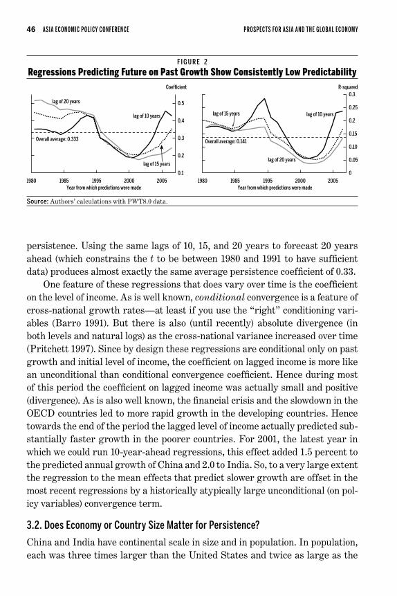
46 ASIA EC ONOMIC P OLICY C ONFERENCE PROSPEC T S FOR ASIA AND THE GLOBAL EC ONOM Y
persistence. Using the same lags of 10, 15, and 20 years to forecast 20 years ahead (which constrains the t to be between 1980 and 1991 to have sufficient data) produces almost exactly the same average persistence coefficient of 0.33.
One feature of these regressions that does vary over time is the coefficient on the level of income. As is well known, conditional convergence is a feature of cross-national growth rates—at least if you use the “right” conditioning vari-ables (Barro 1991). But there is also (until recently) absolute divergence (in both levels and natural logs) as the cross-national variance increased over time (Pritchett 1997). Since by design these regressions are conditional only on past growth and initial level of income, the coefficient on lagged income is more like an unconditional than conditional convergence coefficient. Hence during most of this period the coefficient on lagged income was actually small and positive (divergence). As is also well known, the financial crisis and the slowdown in the OECD countries led to more rapid growth in the developing countries. Hence towards the end of the period the lagged level of income actually predicted sub-stantially faster growth in the poorer countries. For 2001, the latest year in which we could run 10-year-ahead regressions, this effect added 1.5 percent to the predicted annual growth of China and 2.0 to India. So, to a very large extent the regression to the mean effects that predict slower growth are offset in the most recent regressions by a historically atypically large unconditional (on pol-icy variables) convergence term.
3.2. Does economy or Country Size Matter for Persistence?
China and India have continental scale in size and in population. In population, each was three times larger than the United States and twice as large as the
F i G u R e 2
Regressions predicting Future on past growth show Consistently low predictability
Source: Authors’ calculations with PWT8.0 data.
Coefficient
1980 1985 1995 2000 2005Year from which predictions were made
lag of 15 years
lag of 10 years
lag of 20 years
Overall average: 0.333
0.5
0.4
0.3
0.2
0.1
0.3
0.25
0.2
0.15
0.10
0.05
0
R-squared
1980 1985 1995 2000 2005Year from which predictions were made
lag of 15 years lag of 10 years
lag of 20 years
Overall average: 0.141

PRITCHE T T & SUMMERS | ASIAPHORIA MEE T S REGRES SION TO THE ME AN 47
European Union. This leads many to be skeptical as to whether their growth dynamics will be well predicted from cross-national regressions which, even when excluding the tiny economies, contain countries with an average popu-lation less than a typical Indian or Chinese province. However, it is far from obvious that rapid growth episodes are more stable in larger economies mea-sured by either total GDP or population; for example Brazil in 1980 and Japan in 1991, both very large countries, had massive decelerations from rapid growth to extended stagnation, not to mention the recent crisis in the United States.
This empirical question is difficult to address because the usual approach of allowing for interaction terms in size has one of two limitations. Either China and India are included in the regressions, in which case they are often influ-ential data points, or they are excluded, which means that predictions from interactions of size have to extrapolate well out of sample. We choose the latter approach and extend our simple equation to allow for an interaction of persis-tence with size, now pooling across time.
(3) bf bln( ln( ln(g g y S S gt t Ni
t t Ni
ti
ti
ti
t t Ni i) ) ) ) )a b c d { e= + + + + ++ - -, , ,) ) ) .
As a proxy for size we use either total GDP in PPP or population. From sam-ples excluding India and China, the estimated coefficient { is negative and sta-tistically significant, implying that large countries have less persistence. Using either proxy for size, the predicted annual growth rates for the coming decade for both China and India are in the 3 to 4 percent range (Table 8).
3.3. Asymmetry of Persistence: Do booms last while busts Revert?
The question for China and India is primarily the persistence of an already extended episode of rapid growth. It is possible that the reversion to the mean on average is that countries with busts—that is, episodes of low growth—tend to recover to the mean while episodes of rapid growth are more extended. We explore this possibility with the simple exercise of allowing the regression in
TA b l e 8
predicting growth Rates allowing for interactions of growth persistence and Country size
Proxyforsizeinequation(3)(ln) China India 10yrsahead 20yrsahead 10yrsahead 20yrsahead
Total PPP GDP 2.78 3.36 3.02 3.07Population 3.34 4.18 3.68 3.87Source: Authors’ regressions using PWT8.0 data and coefficients from pooled estimates of equation (3) for years 1990–2001 (for 10 year ahead) and 1990–91 (for 20 year ahead).

48 ASIA EC ONOMIC P OLICY C ONFERENCE PROSPEC T S FOR ASIA AND THE GLOBAL EC ONOM Y
each year to have a different coefficient for predicting future growth depend-ing on whether the country’s past growth is above or below the mean of past growth. Since China and India obviously have extended booms, we estimate these regressions without those two countries. The results, presented graph-ically in Figure 3, provide some support for asymmetry. On average for the period 1980–2011 the persistence coefficient was 0.442 for growth above the mean and 0.065 when country growth was below the mean. This suggests that busts were even less persistent than booms—for an extended period the coeffi-cient on past growth was even modestly negative for countries with slow growth, suggesting full regression to the mean.
It is not at all clear how this applies to predicting China’s future growth as, using either growth lagged 10 or 20 years, the very most recent results suggest, if anything, the same or even less persistence of a boom. In any case, the high-est persistence coefficient one could justify using is the period average of 0.44 for growth rates above the mean, which would still imply, all else equal and with 2 percent world growth, decade-ahead growth predictions of roughly 5 percent for China and 3.8 percent for India—still well below the conventional forecasts.
F i G u R e 3
Busts more Rapidly mean-Reverting than Booms on average
Source: Authors’ calculations with PWT8.0 data.
–0.8
–0.7
–0.6
–0.5
–0.4
–0.3
–0.2
–0.1
–0
–0.1
–0.2
Coefficient
1980 1982 1984 1986 1988 1990 1992 1994 1996 1998 2000Year from which predictions are made
growth above mean, lag 20 years
growth above mean, lag 10 years
growth below mean, lag 10 years
growth below mean, lag 20 yearsAverage belowmean: 0.065
Average abovemean: 0.442
PRITCHE T T & SUMMERS | ASIAPHORIA MEE T S REGRES SION TO THE ME AN 49
4. How long Do episodes of Rapid growth usually last? How Do They end?
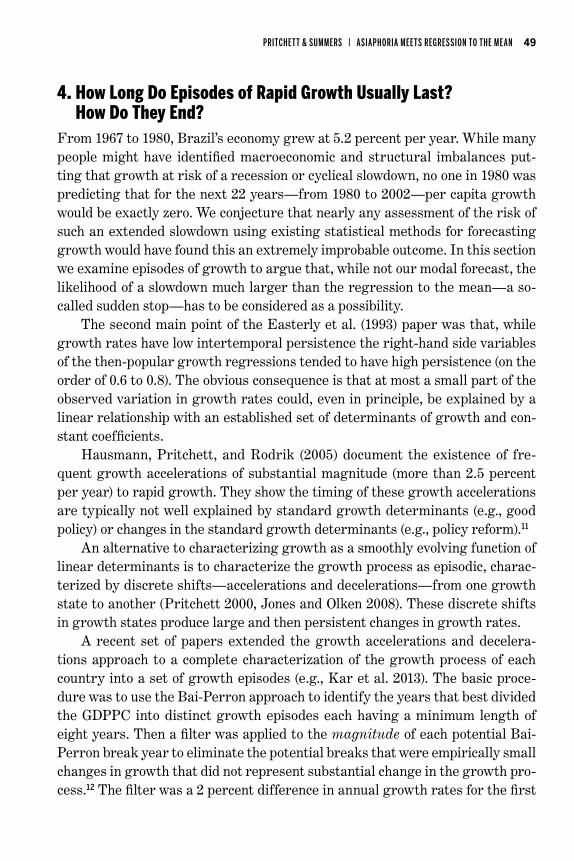
From 1967 to 1980, Brazil’s economy grew at 5.2 percent per year. While many people might have identified macroeconomic and structural imbalances put-ting that growth at risk of a recession or cyclical slowdown, no one in 1980 was predicting that for the next 22 years—from 1980 to 2002—per capita growth would be exactly zero. We conjecture that nearly any assessment of the risk of such an extended slowdown using existing statistical methods for forecasting growth would have found this an extremely improbable outcome. In this section we examine episodes of growth to argue that, while not our modal forecast, the likelihood of a slowdown much larger than the regression to the mean—a so-called sudden stop—has to be considered as a possibility.
The second main point of the Easterly et al. (1993) paper was that, while growth rates have low intertemporal persistence the right-hand side variables of the then-popular growth regressions tended to have high persistence (on the order of 0.6 to 0.8). The obvious consequence is that at most a small part of the observed variation in growth rates could, even in principle, be explained by a linear relationship with an established set of determinants of growth and con-stant coefficients.
Hausmann, Pritchett, and Rodrik (2005) document the existence of fre-quent growth accelerations of substantial magnitude (more than 2.5 percent per year) to rapid growth. They show the timing of these growth accelerations are typically not well explained by standard growth determinants (e.g., good policy) or changes in the standard growth determinants (e.g., policy reform).11
An alternative to characterizing growth as a smoothly evolving function of linear determinants is to characterize the growth process as episodic, charac-terized by discrete shifts—accelerations and decelerations—from one growth state to another (Pritchett 2000, Jones and Olken 2008). These discrete shifts in growth states produce large and then persistent changes in growth rates.
A recent set of papers extended the growth accelerations and decelera-tions approach to a complete characterization of the growth process of each country into a set of growth episodes (e.g., Kar et al. 2013). The basic proce-dure was to use the Bai-Perron approach to identify the years that best divided the GDPPC into distinct growth episodes each having a minimum length of eight years. Then a filter was applied to the magnitude of each potential Bai- Perron break year to eliminate the potential breaks that were empirically small changes in growth that did not represent substantial change in the growth pro-cess.12 The filter was a 2 percent difference in annual growth rates for the first

50 ASIA EC ONOMIC P OLICY C ONFERENCE PROSPEC T S FOR ASIA AND THE GLOBAL EC ONOM Y
potential break; for each subsequent break, if an acceleration followed an accel-eration or if a deceleration followed a deceleration then 1 percent was deemed a break, and if an acceleration followed a deceleration (or vice versa) then a 3 per-cent change was deemed a break. This procedure divides each country’s growth experience into a set of episodes from as few as zero (if the country experiences no growth breaks, as is the case for several OECD countries such as France and the United States) to as many as five, if all four possible Bai-Perron breaks pass the filter (as it does for, say, Argentina).
Figure 4 summarizes growth of India’s real GDP per capita according to PWT7.1 data.13 This characterization of India’s growth regime is an annual growth rate of 2.09 percent from 1950 to 1993, quite near the world average of 2.15 percent. This is followed by an acceleration of growth to 4.23 percent from 1993 to 2002, then a second acceleration of growth from 4.23 to 6.29 from 2002 to 2010. In this set of episodes India has experienced a period of accelerated growth for 17 years (1993 to 2010) at a pace of 4 percent or higher.14
F i G u R e 4
Decomposing india’s growth experiences into Discrete episodes
A GDPPCandCounterfactualUsingEpisodePredicted
B GDPPCandCounterfactualofWorldAverageGrowth
c TotalChangeinIncomeLevelsbyGrowthEpisode(UsingPredicted)
D TotalChangeinIncomeLevelsbyGrowthEpisode(UsingWorldAverage)
Trend (splined)ActualCounterfactual
Ln(GDPPC)
1950 1960 1970 1980 1990 2000 2010
8.4
8.1
7.8
7.5
7.2
6.9
6.6
6.3
Trend (splined)ActualCounterfactual
Ln(GDPPC)
1950 1960 1970 1980 1990 2000 2010
8.4
8.1
7.8
7.5
7.2
6.9
6.6
6.3
Cumulative Change in Ln(GDPPC)
1950 1993 2002 1950–2010
–0.8
–0.7
–0.6
–0.5
–0.4
–0.3
–0.2
–0.1
–0
0.75
0.180.25
0.62
Cumulative Change in Ln(GDPPC)
1950 1993 2002 1950–2010
–0.6
–0.5
–0.4
–0.3
–0.2
–0.1
–0
–0.1–0.03
0.310.28
0.56
Source: Kar et al. (2013).

PRITCHE T T & SUMMERS | ASIAPHORIA MEE T S REGRES SION TO THE ME AN 51
In the graphs the solid black line is the actual data, the dashed line is the predicted growth allowing for splines at each of the identified growth episode transitions, and the gray line is the growth if the country had grown at the pre-dicted rate over each episode. In panel A the predicted growth is from a country/episode-specific regression that allows for regression to the mean and (uncondi-tional) convergence. For example, India’s growth 1993–2002 is predicted from a regression of growth in all other countries from 2002 to 1993 regressed on their growth over the previous episode of 1950 to 1993 and the level of GDPPC in 1993 and then plugging India’s values of growth and level of GDPPC into that regression. This allows for shifts in global growth, duration, and period-specific regression to the mean and convergence (unconditional on anything except past growth). Panel B just uses unweighted world average growth over the episode period as the “predicted” growth.
The same procedure applied to China in Figure 5 produces three accelera-tions in a row. Growth from 1968 to 1977 was 4.33 percent per year, accelerating
F i G u R e 5
Decomposing China’s growth experience into Discrete episodes
A GDPPCandCounterfactualUsingEpisodePredicted
B GDPPCandCounterfactualofWorldAverageGrowth
c TotalChangeinIncomeLevelbyGrowthEpisode(UsingPredicted)
D TotalChangeinIncomeLevelbyGrowthEpisode(UsingWorldAverage)
Source: Kar et al. (2013).
ln(GDPPC)ln(smoothed/spline GDPPC)counterfactual
Ln(GDPPC)
1952 1962 1972 1982 1992 2002
7.4
7.1
6.8
6.5
6.2
5.9
5.6
5.3
ln(GDPPC)ln(smoothed/spline GDPPC)world average(smoothedfrom kinks)
Ln(GDPPC)
1952 1962 1972 1982 1992 2002
7.4
7.1
6.8
6.5
6.2
5.9
5.6
5.3
Cumulative Change in Ln(GDPPC)
1952 1960 1968 1977 1991 1950–2010
–1.6
–1.4
–1.2
–1
–0.8
–0.6
–0.4
–0.2
–0
–0.2
–0.4
0.34
–0.27
0.14
0.81
0.58
1.48
Cumulative Change in Ln(GDPPC)
1952 1960 1968 1977 1991 1950–2010
–2.5
–2
–1.5
–1
–0.5
–0
–0.5
0.09
–0.21
0.13
0.921.21
2.22

52 ASIA EC ONOMIC P OLICY C ONFERENCE PROSPEC T S FOR ASIA AND THE GLOBAL EC ONOM Y
to 7.61 percent from 1977 to 1991 and accelerating yet again in 1991 to 8.63 per-cent until 2010. (The graph goes off the top scale as these figures are produced for a large number of countries with a common vertical axis range in order to allow visual comparability). China has had growth rates of over 6 percent for 33 years starting in 1977, and this data set ends in 2010.
Speculation about how much longer China’s and India’s current episodes of rapid growth might last and what might happen after those episodes, a compar-ison with all other experiences of country accelerations into rapid growth is not dispositive, but it is informative. Table 9 shows all 28 growth recorded accelera-tions that resulted in episodes of growth higher than 6 percent per year (which is roughly two standard deviations above the cross-national mean). This table reveals how unusual China’s (and to a lesser extent India’s) current growth experience is, in three ways.
First, episodes of super-rapid growth (>6 percent) tend to be extremely short-lived. The Kar et al. (2013) method of dating growth episodes mechani-cally does not allow episodes of less than eight years. The median duration of a super-rapid growth episode is nine years, only one year longer than its possi-ble minimum. There are essentially only two countries with episodes even close to China’s current duration. Taiwan had a growth episode from 1962 to 1994 of 6.8 percent (decelerating to growth of 3.5 percent from 1994 to 2010). Korea had an episode from 1962 to 1982 followed by another acceleration in 1982 until 1991 when growth decelerated to 4.48 percent—a total of 29 years of super-rapid growth (>6 percent)—followed by still rapid (>4 percent) growth. So Chi-na’s experience from 1977 to 2010 already holds the distinction of being the only country, quite possibly in the history of mankind, but certainly in the data, to have sustained an episode of super-rapid growth for more than 32 years.
Second, the end of an episode of super-rapid growth is nearly always a growth deceleration. Of the 28 episodes of super-rapid growth, only two ended with a shift to higher growth: Korea in 1982 and China in 1991. So again, China is remarkable in that its acceleration to super-rapid growth in 1977 was fol-lowed by another acceleration in 1991.
Third, the typical (median) end of an episode of super-rapid growth is near complete regression to the world mean growth rate. The median growth of the growth episode that follows an episode of super-rapid growth is 2.1 percent per year. So the “unconditional” expectation (or central tendency) of what will happen following an episode of rapid growth, conditional on a shift in growth, is a reversion to not just somewhat slower growth but massive deceleration of 4.65 percentage points. Such a slowdown is more than twice the cross-national standard deviation of growth rates of roughly 2 percent. A deceleration of that

PRITCHE T T & SUMMERS | ASIAPHORIA MEE T S REGRES SION TO THE ME AN 53
magnitude would take India’s current growth episode of 6.29 to 1.64 percent and China’s from 8.63 (in the episode since 1991) to 3.98 percent.
The results in Table 9 are not an artifact of classifying just super-rapid (>6 percent) growth. If we look at all episodes of growth greater than 4 percent (one standard deviation above mean) we would find many more episodes but similar results about duration and deceleration in all three regards. The 70 episodes of growth above 4 percent (inclusive of those above 6 percent) also have a median
TA b l e 9 all growth episodes above 6 percent per Year,
with Their Duration and growth in the episode Following Yearof Deceleration accelerationto Yearofend Durationof Growthduring Growthafter (negative)/
Country highgrowth ofepisode episode(sofar) highgrowth endof Acceleration episode(>6) episode(sorted) episode (positive)to nextepisode
Trinidad and 2002 Continuing 8 9.80% Continuing TobagoGabon 1968 1976 8 9.26% –2.66% –11.92%Angola 2001 Continuing 9 9.24% ContinuingJapan 1959 1970 11 8.99% –3.40% –5.59%China 1991 Continuing 19 8.63% ContinuingKorea 1982 1991 9 8.40% –4.42% –3.99%Jordan 1974 1982 8 8.18% –4.35% –12.54%Singapore 1968 1980 12 7.94% –4.17% –3.78%Malaysia 1970 1979 9 7.66% –1.52% –6.14%China 1977 1991 14 7.61% –8.63% 1.01%Laos 2002 Continuing 8 7.59% ContinuingMorocco 1960 1968 8 7.25% –3.85% –3.40%Portugal 1964 1973 9 7.10% –1.73% –5.36%Greece 1960 1973 13 6.98% –1.50% –5.48%Taiwan 1962 1994 32 6.77% –3.48% –3.29%Malaysia 1987 1996 9 6.69% –2.10% –4.59%Botswana 1982 1990 8 6.65% –2.80% –3.85%Ecuador 1970 1978 8 6.55% –0.39% –6.94%Thailand 1987 1995 8 6.51% –1.85% –4.65%Ireland 1987 2002 15 6.40% –0.37% –6.03%Cambodia 1998 Continuing 12 6.35% ContinuingIndia 2002 Continuing 8 6.29% ContinuingDominican 1968 1976 8 6.29% –1.01% –5.28% RepublicKorea 1962 1982 20 6.27% –8.40% 2.14%Chile 1986 1997 11 6.16% –2.79% –3.37%Paraguay 1971 1980 9 6.16% –0.66% –5.50%Sierra Leone 1999 Continuing 11 6.11% ContinuingCyprus 1975 1984 9 6.04% –3.81% –2.24%Median 9 6.87% –2.10% –4.65%Source: Pritchett et al. (2013).

54 ASIA EC ONOMIC P OLICY C ONFERENCE PROSPEC T S FOR ASIA AND THE GLOBAL EC ONOM Y
duration of nine years. One does find more examples of extended rapid growth at greater than 4 percent—Singapore with 30 years at 4.17 percent from 1980 to 2010, Indonesia with 29 years at 4.71 percent from 1967 to 1996, Thailand with 29 years at 4.91 percent from 1958 to 1987 (followed by an acceleration), and Vietnam with 21 years (and ongoing) at 5.54 percent. But still, other than the combination of Thailand’s episodes (the first of which was at much lower rates than China’s and the end of which precipitated the East Asian crisis of 1997), none of the episodes of even rapid growth (>4 percent) is of longer dura-tion than China’s. In the 70 episodes of rapid growth (>4 percent) there are only four cases in which the episode ended with a growth shift that was an acceler-ation (China in 1991, Korea in 1982, Thailand in 1987, and Botswana in 1982). Finally, the median growth in the episode following the rapid growth episodes is 1.85 percent. Again, the growth following an episode of rapid growth is, on average, full regression to the mean.
4.1. Are Asian Giant Growth Dynamics Driven by a Middle income Trap?
In a set of influential papers, Eichengreen, Park, and Shin (2012, 2013) have argued for the existence of a middle-income trap. Their analysis identifies epi-sodes of slowdown in middle-income countries as countries with an episode of growth greater than 3.5 percent followed by a growth deceleration of 2 percent or more, which were also defined as middle income by a level of PPP income of 10,000. Their 2012 paper suggested a mode in the distributions of slowdown around PPP15,000–16,000. Their 2013 update using the new PWT7.1 data with more observations altered both their identifications of the growth breaks, modified some conclusions, and added some insights. First, they find less evi-dence of a single mode and more suggestion of two modes of slowdowns, one at PPP10,000–11,000 and another at PPP15,000–16,000. Second, they examine the correlates of slowdowns and find that education of secondary and higher levels (conditional on GDP per capita) and high technology exports mitigate the risks of slowdown.
The Eichengreen, Park, and Shin analysis focuses only on those decelera-tions among countries that are middle income and hence limit their sample to decelerations among countries that are already near middle income. The mid-dle-income trap conjecture almost certainly has no bearing on India, which is and will remain for the foreseeable future a poor country. The PWT8.0 estimate of real GDP (expenditure) per capita is $3755—which is only 8.4 percent of the U.S. level.
We replicate a version of the middle-income trap analysis by taking all structural breaks identified by Kar et al. (2013) and identifying those that are
PRITCHE T T & SUMMERS | ASIAPHORIA MEE T S REGRES SION TO THE ME AN 55
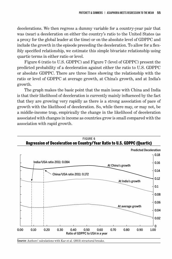
decelerations. We then regress a dummy variable for a country-year pair that was (near) a deceleration on either the country’s ratio to the United States (as a proxy for the global leader at the time) or on the absolute level of GDPPC and include the growth in the episode preceding the deceleration. To allow for a flex-ibly specified relationship, we estimate this simple bivariate relationship using quartic terms in either ratio or level.
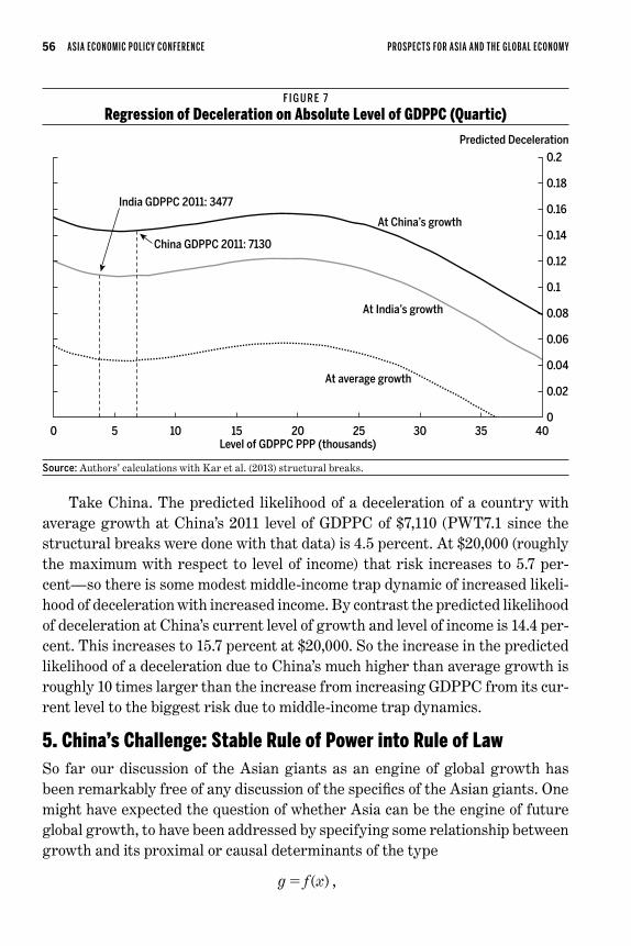
Figure 6 (ratio to U.S. GDPPC) and Figure 7 (level of GDPPC) present the predicted probability of a deceleration against either the ratio to U.S. GDPPC or absolute GDPPC. There are three lines showing the relationship with the ratio or level of GDPPC at average growth, at China’s growth, and at India’s growth.
The graph makes the basic point that the main issue with China and India is that their likelihood of deceleration is currently mainly influenced by the fact that they are growing very rapidly as there is a strong association of pace of growth with the likelihood of deceleration. So, while there may, or may not, be a middle-income trap, empirically the change in the likelihood of deceleration associated with changes in income as countries grow is small compared with the association with rapid growth.
F i G u R e 6
Regression of Deceleration on Country/Year Ratio to u.s. gDppC (Quartic)
Source: Authors’ calculations with Kar et al. (2013) structural breaks.
0.18
0.16
0.14
0.12
0.1
0.08
0.06
0.04
0.02
0
Predicted Deceleration
0.00 0.10 0.20 0.30 0.40 0.50 0.60 0.70 0.80 0.90 1.00Ratio of GDPPC to USA in a year
At China’s growth
At India’s growth
At average growth
China/USA ratio 2011: 0.172
India/USA ratio 2011: 0.084
56 ASIA EC ONOMIC P OLICY C ONFERENCE PROSPEC T S FOR ASIA AND THE GLOBAL EC ONOM Y
Take China. The predicted likelihood of a deceleration of a country with average growth at China’s 2011 level of GDPPC of $7,110 (PWT7.1 since the structural breaks were done with that data) is 4.5 percent. At $20,000 (roughly the maximum with respect to level of income) that risk increases to 5.7 per-cent—so there is some modest middle-income trap dynamic of increased likeli-hood of deceleration with increased income. By contrast the predicted likelihood of deceleration at China’s current level of growth and level of income is 14.4 per-cent. This increases to 15.7 percent at $20,000. So the increase in the predicted likelihood of a deceleration due to China’s much higher than average growth is roughly 10 times larger than the increase from increasing GDPPC from its cur-rent level to the biggest risk due to middle-income trap dynamics.
5. China’s Challenge: stable Rule of power into Rule of lawSo far our discussion of the Asian giants as an engine of global growth has been remarkably free of any discussion of the specifics of the Asian giants. One might have expected the question of whether Asia can be the engine of future global growth, to have been addressed by specifying some relationship between growth and its proximal or causal determinants of the type
( )g f x= ,
F i G u R e 7
Regression of Deceleration on absolute level of gDppC (Quartic)
Source: Authors’ calculations with Kar et al. (2013) structural breaks.
0.2
0.18
0.16
0.14
0.12
0.1
0.08
0.06
0.04
0.02
0
Predicted Deceleration
0 5 10 15 20 25 30 35 40Level of GDPPC PPP (thousands)
At China’s growth
At India’s growth
At average growth
China GDPPC 2011: 7130
India GDPPC 2011: 3477

PRITCHE T T & SUMMERS | ASIAPHORIA MEE T S REGRES SION TO THE ME AN 57
and then making the case for continued rapid growth or deceleration based on that model and the likely trajectories of the x variables. While we will engage in some country-specific discussion along those lines below, we deliberately choose not to go that direction for three reasons.
First, conditional forecasting of this type is only as good as the forecasts of the conditioning variables. Imagine dividing the potential x’s into two types: those easy to forecast because they have high persistence (e.g., size of the coun-try, geography, latitude, nearness to ports) and those with low persistence. Obvi-ously the former are quite easy to forecast, but also cannot be the usual causes of super-rapid growth. Hence they would only be good at predicting the mean that super-rapid growth is likely to regress to, but because they are highly per-sistent they would have fairly low explanatory power for changes in growth as these variables must, by definition as high persistence variables, have fairly low explanatory power for changes in growth. That is, econometrically, if serial correlation of growth is low then constant determinants of growth cannot have high explanatory power.
The growth determinants with low persistence may be good at forecasting growth but are themselves harder to forecast. Again, by construction, extrapo-lation of those variables is a bad forecast of x, making a forecast conditional on x a bad forecast. To use this forecast continued rapid growth would then require that we somehow have a good forecast that some important growth determinant is going to change in such a way that growth that otherwise would have decel-erated remains rapid. We cannot think of such a thing and, as we argue below, there are several prominent possibilities of just the opposite dynamic.
Second, even if we could reliably forecast the x’s we would also have to imag-ine we had identified a reasonably accurate and long-term stable empirical rela-tionship. This just has not been true to any extent in the domain of economic growth, nor is this unique to economic growth. We have lived through a series of major political, social, and economic events in our lifetime, none of which were widely predicted by experts in the appropriate domain.
A salient recent example is that we are still living in the shadow of the finan-cial crisis in the United States and elsewhere. It is worth pointing out that the depth and severity of the crisis was not only not predicted by academic econ-omists on the sidelines nor, in their assessments of the riskiness of classes of assets, by raters (Silver 2012) nor by policymakers. People who had incredibly high stakes on correct forecasts by having most of their financial wealth at risk (and, unfortunately, leveraged) misforecast the outcomes in the housing mar-ket badly—for them. This is not because there was ignorance of a housing bub-ble; some mainstream economists (particularly Robert Shiller among others)

58 ASIA EC ONOMIC P OLICY C ONFERENCE PROSPEC T S FOR ASIA AND THE GLOBAL EC ONOM Y
pointed out the magnitude of the deviation of housing prices from their long-run trends early (at least by 2005) and often. But what was missed was how this would translate into the financial sector and the economy as a whole. Leamer’s (2010) demonstration of how the evolution of prices and quantities in the Los Angeles housing market produced enormously different dynamics in different periods, such that the confidence intervals based on past data for future predic-tions substantially understated the true range of possibility is just one example of the instability of models.
Third, super-rapid growth is due in part to a large residual or unexplained component, which we rarely admit as we overexplain the current reality. While perhaps too much can be made of Taleb’s (2007) “Black Swan” arguments that we overpredict reality—that is, we concoct reasons ex post to make it seem as if we understand what happened when we really didn’t—conventionally too lit-tle is made of it. Taleb’s obvious and poignant example that, while Lebanon remained an oasis of multireligious peaceful coexistence and institutional suc-cess (aka “the Switzerland of the Middle East”) there were many powerful the-ories why Lebanon’s success was overdetermined by observable factors. After Lebanon was engulfed by the general regional instability, it quickly became equally obvious that Lebanon was doomed to instability.
Dramatic changes in perceptions of the Japanese economic system provide another example. During the late 1980s, it was widely believed that Japanese-style industrial policy, Japanese emphasis on corporate linkages through keiretsu, and high levels of investment supported by financial repression were keys to rapid growth. A decade later all of these conclusions had been abandoned to be replaced by nearly opposite views in the conventional wisdom.
At an even broader level, it was widely believed in the early 1960s that the Soviet Union would quite likely outstrip the United States economically based on an extrapolation of its recent growth performance. Justifications were even developed for the apparently rapid growth of central Europe as late as 1979, as illustrated by the famous World Bank report of that year on the Romanian eco-nomic miracle.
The point can be demonstrated for countries as well. We believe that in the United States there are no known examples since 1950 when the consensus forecast called for recession one year out, even though recessions have occurred on average every five or six years since then and even though they appear to have a permanent rather than a temporary impact on output.
Imagine that in a conference in 2023 we know ex post that in 2014 Chi-na’s GDPPC growth was 8 percent for the calendar year 2014. However, we also know that in March 2015 China experienced a sudden sharp slowdown in

PRITCHE T T & SUMMERS | ASIAPHORIA MEE T S REGRES SION TO THE ME AN 59
economic growth that persisted and caused growth to be only 2 percent from 2015 to 2023. Here is the question: In that scenario, what do we think the fore-cast of growth 2015–23 was in the IMF World Economic Outlook for China in October 2014, six months before the slowdown? Our guess is that the 2014 forecast was 8 percent growth and was expressed with substantial confidence.
All that said, we suspect that the reasons slowdowns will come in China and India are similar but will manifest differently given the very different politics. That is, in neither country does investor confidence rely on rule of law. In both countries there are plausible scenarios in which the current political settlement that provides a climate for ordered deals (Hallward-Driemeier and Pritchett 2011) will be disrupted. This disruption of the arrangements that provide set-tled expectations of investors can easily create processes with nonlinear sud-den stops.
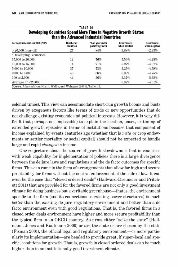
As North, Wallis, and Weingast (2009) show, the reason for the low growth on average of developing versus developed countries is not the lack of rapid growth—it is the lack of the persistence of that growth and the very low growth rates during their periods of negative growth. As we saw with Denmark, the rich industrial countries are rich because they grew at modest rates for very long periods, with little variation and few disastrous downturns—e.g., 84 per-cent of years in positive growth, and negative growth only falling to –2.33 percent per year. By contrast, current poor countries have failed to converge because they grow much faster when they are growing (e.g., 5.39 percent per year for those in the 2,000 to 5,000 range) then a third of their time have sizable negative growth (averaging –4.75 percent for the same grouping).
Take for example the comparison of the rich countries with those countries with a per capita income between $2,000 and $5,000. Average growth is equal to the average growth when positive times the probability that growth is posi-tive plus average growth when negative times the probability of growth being negative. For both groups, average growth when positive contributes just about 3.6 percent to the weighted average. But for poorer countries, average growth when negative contributes –1.6 percent rather than –0.4 percent, accounting for all the difference in growth (Table 10).
Powerful evidence suggests that high levels of output per capita are asso-ciated with high levels of institutional quality (e.g., Hall and Jones 1999, Ace-moglu, Johnson, and Robinson 2001, and North, Wallis, and Weingast 2009) and that, over very long periods, this association is sustained so that institutional arrangements can have very long-lasting effects (including regional evidence within countries as in Dell (2010) showing the persistence on levels of income and well-being today in Peru and Bolivia of the mita arrangements in Spanish
60 ASIA EC ONOMIC P OLICY C ONFERENCE PROSPEC T S FOR ASIA AND THE GLOBAL EC ONOM Y
colonial times). This view can accommodate short-run growth booms and busts driven by exogenous factors like terms of trade or new opportunities that do not challenge existing economic and political interests. However, it is very dif-ficult (but perhaps not impossible) to explain the location, onset, or timing of extended growth episodes in terms of institutions because that component of income explained by events centuries ago (whether that is mita or crop endow-ments or settler mortality or social capital) should not be expected to handle large and rapid changes in income.
One conjecture about the source of growth slowdowns is that in countries with weak capability for implementation of policies there is a large divergence between the de jure laws and regulations and the de facto outcomes for specific firms. This can come in the form of arrangements that allow for high and secure profitability for firms without the neutral enforcement of the rule of law. It can even be the case that “closed ordered deals” (Hallward-Dreimeier and Pritch-ett 2011) that are provided for the favored firms are not only a good investment climate for doing business but a veritable greenhouse—that is, the environment specific to the firm (and its connections to existing power structures) is much better than the existing de jure regulatory environment and better than a de facto environment even with good regulations. That is, the favored firms in a closed order deals environment have higher and more secure profitability than the typical firm in an OECD country. As firms either “seize the state” (Hell-mann, Jones and Kaufmann 2000) or are the state or are chosen by the state (Fisman 2001), the official legal and regulatory environment—or more partic-ularly its implementation—are bended to provide great, if super-local and spe-cific, conditions for growth. That is, growth in closed ordered deals can be much higher than in an institutionally good investment climate.
TA b l e 1 0
Developing Countries spend more Time in negative growth states than the advanced industrial Countries
Percapitaincomein2000(PPP) Numberof %ofyearswith Growthrate, Growthrate, countries positivegrowth whenpositive whennegative
>20,000 (non–oil) 27 84% 3.88% –2.33%“Developing” countries15,000 to 20,000 12 76% 5.59% –4.25%10,000 to 15,000 14 71% 5.27% –4.07%5,000 to 10,000 37 73% 5.25% –4.59%2,000 to 5,000 46 66% 5.39% –4.75%300 to 2,000 44 56% 5.37% –5.38%Average of <20,000 5.37% –4.61%Source: Adapted from North, Wallis, and Weingast (2009), Table 1.2.

PRITCHE T T & SUMMERS | ASIAPHORIA MEE T S REGRES SION TO THE ME AN 61
But, the difficulty is the transition. Since investor expectations (both domes-tic and foreign) are grounded in specific relationships to specific power bases, shifts in power can occasion very sudden stops as investor expectations have to realign to new realities. This can create sudden stops that then can resume as new conditions are established or can persist for a very long time if new institu-tions have to emerge and have credibility.
This can lead measures of institutions—like those that measure political institutions—to be associated with the range of growth outcomes, not neces-sarily the level of growth over medium-run periods. Figure 8 shows the largest difference in growth rates over 10-year periods of countries at various levels of the Polity score (which measures autocracy/democracy on a –10 to +10 scale). While autocracies can maintain very high growth rates—even over extended periods—they also tend to have much larger ranges of growth outcomes—with booms and busts—than stable democracies.
There is a strong cross-national relationship between the extent to which a country is (or is rated as) a democracy and GDP per capita. This relationship reveals nothing about cause and effect, and certainly we are not going to assert some strong, monocausal, linear dynamic whereby richer countries naturally
F i G u R e 8
lower polity scores associated with larger Changes in growth over Time
Source: Pritchett and Werker (2012).
AFG
AGOALB
ARG
AUS
AUT
BDI
BELBEN
BFABGD
BGRBHR
BOL
BRABTN
BWA
CAFCANCHE
CHLCHN
CIV
CMR COG
COL
COMCRI
CUB
CYP
DJI
DNK
DOMDZA
ECU
EGY ESP
ETHFIN
FJI
FRA
GAB
GBR
GHA
GIN
GMB
GNB
GRCGTM
GUY
HND
HTIHUNIDN
IND
IRL
IRNIRQ
ISRITA
JAM
JOR
JPN
KEN
KHM
KOR
KWT
LAO
LBN
LBY
LKALSO
MAR
MDGMEXMLI
MNG
MOZ
MRT
MUS
MWIMYS NAMNER
NGANIC
NLDNORNPL
NZL
OMN
PAKPAN
PER
PHL
PNG
POL PRTPRY
QATROM
RWA
SAU
SDN
SEN
SGP
SLB
SLE
SLVSOM
SVK
SWE
SWZSYR
TCDTGO
THA
TTO
TUN TUR
TWNTZA
UGA
URY
USA
VEN
VNM ZAF
ZARZMB
ZWE
0.25
0.2
0.15
0.1
0.05
0
Biggest Change in Growth, 10 year periods
–10 –5 0 5 10Average Polity
Autocracies Muddle Democracy

62 ASIA EC ONOMIC P OLICY C ONFERENCE PROSPEC T S FOR ASIA AND THE GLOBAL EC ONOM Y
become more democratic. That said, Figure 9 shows the relationship between a stock-like measure of democratic capital index that cumulates the Polity score into a stock (to smooth the transitory fluctuations) which then scales most dem-ocratic countries as 100 and least democratic countries as 0.
The obvious point is that there are extremely few exceptions to the ten-dency for all countries with high levels of GDP per capita (expressed here as an index from 0 to 100) to also have high levels of (measured) democracy. The only two exceptions for a country with GDPPC more than a third of the leader (33 on the index) not having a democracy capital score above 80 are Oman (an oil producer)15 and Singapore. For countries in China’s current range of output (between 10 and 25 on scale of 0 to 100), the complete range of democracy out-comes exist. However, the average for this group is a democracy capital index of 71 with a standard deviation of 25. Already at a score of 14, China is much less democratic than the typical country with its level of output.
For China to continue to have rapid economic growth while maintaining its current level of democracy (as proxied by its Polity score)—a trajectory moving rapidly due east in Figure 9—would make it more and more anomalous. Which is not to say it isn’t possible. Singapore (granted, a small city-state of only 5
F i G u R e 9
Relationship between gDp per Capita and a stock of Democracy Capital index, 2008 (both normalized 0 to 100)
Source: Kenny and Pritchett (2013).
AFG
AGO
ALB
ARG
AUSAUT
BDI
BEL
BEN
BFA
BGD
BGRBOL
BRABWA
CAF
CAN CHE
CHL
CHNCIV
CMRCOG
COL
CRI
CUB
CYP DEUDNK
DOM
DZA
ECU
EGY
ESP
ETH
FIN
FJI
FRA
GAB
GBR
GHA
GINGMB
GNB
GRC
GTM
GUY
HND
HTI
HUN
IDN
INDIRL
IRN
IRQ
ISR ITAJAM
JOR
JPN
KEN
KHM
KOR
LAO
LBNLBR
LKA
LSO
MAR
MDG MEXMLI
MNG
MOZ
MRT
MUS
MWIMYS
NAM
NER
NGA
NIC
RONDLN
NPL
NZL
OMN
PAK
PAN
PERPHL
PNG
POL
PRT
PRYROM
RWASDN
SEN
SGP
SLE
SLV
SOM
SWE
SWZ
SYR
TCDTGO
THA
TTO
TUN
TUR TWN
TZAUGA
URYUSA
VEN
VNM
ZAF
ZAR
ZMB
ZWE
100
90
80
70
60
50
40
30
20
10
0
Polity Capital
0 10 20 30 40 50 60 70 80 90 100GDPPC

PRITCHE T T & SUMMERS | ASIAPHORIA MEE T S REGRES SION TO THE ME AN 63
million people) has managed to be nearly the richest country in the world while only having a Polity democracy capital index of 40. But even 40 is more than twice China’s current level of 14.
An empirical question is, What, if any, impact might we expect a democra-tizing period to have on China’s growth?
A huge literature examines the association between democracy and growth, and generally finds only a weak and non-robust association between the level of democracy and the pace of growth but that less-democratic countries tend to have much higher volatility of growth. However, a simple analysis of whether democracies grow faster or slower than non-democracies does not capture the possibility that large political transitions may themselves have impacts. In this case, while democracies may be capable of sustaining rapid growth in the long run, the transition itself may create an adjustment period of slow growth. To examine this question, we need to compare countries’ growth rates before and after large, rapid political transitions from autocracy to democracy. For this, we need to define what qualifies as “large” democratizing transitions.
Pritchett (2011) searched the Polity data to identify all instances in which a country’s index had increased by more than five units in a single year towards less autocracy or more democracy. These were the candidates for a large dem-ocratic transition. He then used a decision tree to classify and date these potential transitions, addressing in particular the treatment of countries with multiple transitions. This classification scheme resulted in 52 episodes of large democratic transition. Once large democratic transitions had been identified, the next step was to calculate growth rates before and after the transition.16 To capture the medium- to long-run dynamics term, he calculated the growth rate for the 10-year period ending three years before the transition and that for the 10-year period beginning one year after the transition (or, if 10 years of data were not available, until the data ended). For instance, in the case of Indonesia, the two 10-year periods would be 1986–96 (the period ending three years before the democratic transition in 1999) and 2000–07 (the period beginning one year after the transition and ending when the PWT6.3 data stop in 2007).17
The first result evident in Table 11 is that nearly every country that expe-rienced a large democratic transition after a period of above-average growth (more than the cross-country average of 2 percent) experienced a sharp decel-eration in growth in the 10 years following the democratizing transition. Among 22 countries in which episodes of large democratic transition coincided with above-average growth, all but one (Korea in 1987 with an acceleration of only 0.22 percent) experienced a growth deceleration. The combination of high ini-tial growth and democratic transition seems to make some deceleration all but

64 ASIA EC ONOMIC P OLICY C ONFERENCE PROSPEC T S FOR ASIA AND THE GLOBAL EC ONOM Y
inevitable. The magnitude of the decelerations was very large: The median deceleration across the 22 countries was 2.99 percent, and the average deceler-ation was 3.53 percent.
At least one mechanism that could cause democratizing transitions to decel-erate growth has been explored in the case of Indonesia. As Fisman (2001) has shown, the stock market value of firms connected to President Suharto was associated with news about his health, implying that a substantial amount of their value was related to his personal control of the levers or power. While power in China is obviously controlled by much larger and broader regionally competing forces, it nevertheless is not exercised in what one would typically call a democratic fashion nor according to the rule of law, nor are tradition-ally conceived human rights protected. That said, the fact that China is rated by most indicators as having very low control over corruption and not having
TA b l e 1 1 Countries with large Democratic Transitions starting from above average
(2 percent per Year) growth in gDp per Capita 10-yeargrowth 10-yeargrowth Changeinpre-/
Country Yearof Magnitudeof ending3years beginning1year post-transition transition Polityincrease beforedemocratizing aftertransition(%) growthrates(%) transition(%)
Greece 1975 7 7.19 0.02 –7.17Iran 1979 10 7.11 0.11 –7.01Portugal 1976 6 7.11 1.48 –5.63Taiwan 1992 8 6.47 3.95 –2.52Taiwan 1987 6 6.42 5.78 –0.64Nigeria 1979 7 5.81 –2.44 –8.25Ecuador 1979 14 5.69 –1.66 –7.36Congo 1992 6 5.68 0.57 –5.11Indonesia 1999 11 5.54 3.28 –2.26Dominican Rep. 1978 9 5.50 1.35 –4.14South Korea 1987 6 5.36 5.57 0.22Thailand 1992 10 4.67 0.82 –3.85Mongolia 1990 9 4.39 2.09 –2.30Bulgaria 1990 15 4.02 –0.10 –4.12Panama 1989 16 3.91 1.68 –2.23Benin 1990 7 3.62 1.30 –2.32Pakistan 1988 12 3.50 1.32 –2.18Uruguay 1985 16 3.44 3.16 –0.27Brazil 1985 10 3.31 –0.34 –3.65Paraguay 1989 10 2.70 –0.75 –3.45Bolivia 1982 15 2.37 0.27 –2.09Romania 1989 6 2.14 0.85 –1.28Median 5.01 1.08 –2.99Average 4.82 1.29 –3.53Source: Pritchett (2011).
PRITCHE T T & SUMMERS | ASIAPHORIA MEE T S REGRES SION TO THE ME AN 65
improved over the previous decade has obviously not been an obstacle to rapid growth. This is not surprising as Shleifer and Vishny (1993) have long argued that organized corruption need not be inimical to growth. However it is difficult for corruption to remain organized during a transition in political power.
We are not forecasting that China will move towards democracy nor that this will be what causes China’s growth to slow. But we are pointing out the very dangerous shoals through which the Chinese economy is currently sailing very rapidly. While it is possible to envision the transition not happening for some extended time, and while it is possible to envision the transition being made smoothly, neither of these are the outcomes typically observed in the data.
6. ConclusionMuch analysis and forecasting regarding economic growth treats a country’s history as the principle information for thinking about its future. It is an empir-ical question whether this is right or wrong. Someone looking to predict the future health status of a 60-year-old would give some weight to her health his-tory but probably much more weight to the available information on the past populations of 60-year-olds. In the same way, our findings suggest that in fore-casting growth rates over the long term, forecasters should give heavy weight to the growth rate of all countries. We believe that most economic forecasting errors historically have come from neglecting this principle and placing exces-sive weight on a country’s recent past in making forecasts. Perhaps this is why official forecasts usually miss discontinuities.
The recovery in the United States is currently slow relative to expectations, and the recovery in Europe is even weaker. Yet, the post-crisis fallout for the global economy has been much less than feared. This has certainly been due in large part to sustained growth in China and India that likely has positive spill-overs (e.g., through high commodity prices and trade linkages) to other econo-mies. The hopeful and in many quarters prevailing view is that this represents a decisive shift and that rapid global growth will continue—and perhaps even OECD growth will recover—with Asia as the engine, via the Asian giants and others.
This is certainly one scenario.However, those around the age of the authors or older remember well at
least two previous periods of Asiaphoria. Japan’s rapid growth from the 1960s (though decelerated already by the 1970s) led to popular and academic litera-ture explaining why Japan succeeded and would continue to succeed. Although there were some concerns about a bubble in Japanese real estate, almost no one predicted in 1991 that Japan’s real GDP per capita would be only 12 percent

66 ASIA EC ONOMIC P OLICY C ONFERENCE PROSPEC T S FOR ASIA AND THE GLOBAL EC ONOM Y
higher in 2011 than 20 years earlier (an annual growth rate of only 0.6 percent) and that total factor productivity in Japan, which had doubled from 1961 to 1991 would be 6 percent lower in 2011 than in 1991 (data and calculations from PWT8.0).
The second Asiaphoria was the growth in the 1990s when Southeast Asian countries—Indonesia, Malaysia, and Thailand—appeared to be booming along with the Four Dragons. A financial and economic crisis spread across East Asia in the late 1990s with sharp contractions in nearly all the booming economies. While most recovered quickly, the annual growth rates for the most recent epi-sode of growth have been only 1.42 percent for Indonesia, 2.1 percent for Malay-sia, and 1.85 percent for Thailand, which is a relatively rapid growth from a quite steep contraction. Korea and Taiwan had shorter crises and quicker recoveries, but their growth rates in the more recent growth episode are 3.48 and 3.29 per-cent, respectively, which is rapid but nothing like the current growth of China or India.
Regression to the mean is the single most robust finding of the growth liter-ature, and the typical degrees of regression to the mean imply substantial slow-downs in China and India relative even to the currently more cautious and less bullish forecasts.
India and, even more so, China are experiencing historically unprecedented episodes of growth. China’s super-rapid growth has already lasted three times longer than a typical episode and is the longest ever recorded. The ends of epi-sodes tend to see full regression to the mean, abruptly.
It is impossible to argue that either China or India have the kinds of qual-ity institutions that have been associated with the steady dynamic of growth in the currently high productivity countries. The risks of sudden stops are much higher with weak institutions and organizations for policy implementation. China and India have very different modalities of this risk, but both have tricky paths to continued prosperity.
We would suggest several implications of these conclusions. First, there will be a strong tendency to assume that, if growth slows substantially in China or India, it will represent an important policy failure. This is not right. Regression to the mean in a decade or so is the rule, not the exception. What would require much more explanation would be continued rapid growth, which would be very much outside the general run of experience. Second, those making global pro-jections should allow a very wide confidence interval with respect to growth for countries whose current growth rates are far from the mean. Given the sensitiv-ity of commodity demands in particular to growth rates in Asia, this suggests substantial uncertainty about the medium-term path of commodity prices. In
PRITCHE T T & SUMMERS | ASIAPHORIA MEE T S REGRES SION TO THE ME AN 67
the same way, forecasts of global energy use and climate change impacts should also recognize the possibility of discontinuities in Asia. Third, much geopolitical analysis has focused on the implications of a rising China, and certainly Chinese international relations theorists have extensively studied past rising powers. Contingency planning should also embrace scenarios in which Chinese growth slows dramatically, presumably bringing with it a range of domestic and inter-national political implications.
RefeRences
Acemoglu, Daron, Simon Johnson, and James Robinson. 2001. “The Colonial Origins of Comparative Development: An Empirical Investigation.” American Economic Review 91(5), pp. 1,369–1,401.
Aguiar, Mark, and Gita Gopinath. 2007. “Emerging Markets Business Cycles: The Cycle Is the Trend.” Journal of Political Economy 115, pp. 69–102.
Barro, Robert. 1991. “Economic Growth in a Cross Section of Countries.” Quarterly Journal of Economics 102(2), pp. 407–443.
Breuer, Janice Boucher, and John McDermott. 2013. “Economic Depression in the World.” Journal of Macroeconomics 38(PB), pp. 227–242.
Dell, Melissa. 2010. “The Persistent Effects of Peru’s Mining Mita.” Econometrica 78(6), pp. 1,863–1,903.
Easterly, William, Michael Kremer, Lant Pritchett, and Lawrence Summers. 1993. “Good Policy or Good Luck: Country Growth Performance and Temporary Shocks.” Journal of Monetary Economics 32(3), pp. 459–483.
Eichengreen, Barry, Donghyun Park, and Kwanho Shin. 2012. “When Fast Growing Econo-mies Slow Down: International Evidence and Implications for China.” Asian Economic Papers 11, pp. 42–87.
Eichengreen, Barry, Donghyun Park, and Kwanho Shin. 2013. “Growth Slowdown Redux: New Evidence on the Middle Income Trap.” NBER Working Paper 18673.
Feenstra, Robert C., Robert Inklaar, and Marcel Timmer. 2013. “The Next Generation of the Penn World Table.” NBER Working Paper 19255.
Fisman, Raymond. 2001. “Estimating the Value of Political Connections.” American Economic Review 91(4), pp. 1,095–1,102.
Fogel, Robert. 2010. “123,000,000,000,000.” Foreign Policy, December 20.
Greenspan, Alan. 2013. The Map and the Territory: Risk, Human Nature, and the Future of Forecasting. New York: Penguin Press.
Hall, Robert, and Charles I. Jones. 1999. “Why Do Some Countries Produce So Much More Output Per Capita Than Others?” Quarterly Journal of Economics 114(1), pp. 83–116.

68 ASIA EC ONOMIC P OLICY C ONFERENCE PROSPEC T S FOR ASIA AND THE GLOBAL EC ONOM Y
Hallward-Driemeier, Mary, and Lant Pritchett. 2011. “How Business Is Done and the ‘Doing Business’ Indicators: The Investment Climate When Firms Have Climate Con-trol.” World Bank Policy Research Working Paper 5563.
Hausmann, Ricardo, Lant Pritchett, and Dani Rodrik. 2005. “Growth Accelerations.” Journal of Economic Growth 10(5), pp. 303–329.
Hellman, Joel, Geraint Jones, and Daniel Kaufmann. 2000. “Seize the State, Seize the Day: State Capture, Corruption, and Influence in the Transition.” World Bank Policy Research Working Paper 2444.
Jones, Benjamin, and Benjamin Olken. 2008. “The Anatomy of Start-Stop Growth.” Review of Economics and Statistics 90(3), pp. 582–587.
Kar, Sabyasachi, Lant Pritchett, Selim Raihan, and Kunal Sen. 2013. “Looking for a Break: Identifying Transitions in Growth Regimes.” Journal of Macroeconomics 38(PB), pp. 151–166.
Kenny, Charles, and Lant Pritchett. 2013. “Promoting Millennium Development Ideals: The Risks of Defining Development Down.” Center for Global Development Working Paper 338.
Leamer, Edward. 2010. “Tantalus on the Road to Asymptopia.” Journal of Economic Perspectives 24(2), pp. 31–46.
Levine, Ross, and David Renelt. 1992. “A Sensitivity Analysis of Cross-Country Growth Regressions.” American Economic Review 82(4), pp. 942–963.
North, Douglas, John Wallis, and Barry Weingast. 2009. Social Order: A Conceptual Framework for Interpreting Recorded Human History. Cambridge: Cambridge Uni-versity Press.
Organisation for Economic Co-Operation (OECD). 2012. Looking to 2060: LongTerm Global Growth Prospects. OECD Economic Policy Paper 03.
Pritchett, Lant. 1997. “Divergence, Big Time.” Journal of Economic Perspectives 11(3), pp. 3–17.
Pritchett, Lant. 2011. “How Good Are Good Transitions? Indonesia after Suharto, for Instance.” Working paper, Harvard University.
Pritchett, Lant. 2000. “Understanding Patterns of Economic Growth: Searching for Hills among Mountains, Plateaus, and Plains.” World Bank Economic Review 14(2), pp. 221–250.
Pritchett, Lant, and Eric Werker. 2012. “Developing the Guts of a Gut (Grand Unified The-ory): Elite Commitment and Inclusive Growth.” Effective States and Inclusive Develop-ment Research Centre (ESID) Working Paper 16/12.
Rodríguez, Francisco, and Cameron A. Shelton. 2013. “Cleaning Up the Kitchen Sink: Spec-ification Tests and Average Derivative Estimators for Growth Econometrics.” Journal of Macroeconomics 38, pp. 260–273.
Rodrik, Dani. 1999. “Where Did All the Growth Go? External Shocks, Social Conflict, and Growth Collapses.” Journal of Economic Growth 4(December), pp. 358–412.

PRITCHE T T & SUMMERS | ASIAPHORIA MEE T S REGRES SION TO THE ME AN 69
Rodrik, Dani, and Arvind Subramanian. 2004. “From ‘Hindu Growth’ to Productivity Surge: The Mystery of the Indian Growth Transition.” NBER Working Paper 10376 (March).
Rodrik, Dani, and Romain Wacziarg. 2005. “Do Democratic Transitions Produce Bad Eco-nomic Outcomes?” American Economic Review 95(2), pp. 50–55.
Sala-i-Martin, Xavier. 1997. “I Just Ran Four Million Regressions.” NBER Working Paper 6252.
Shleifer, Andrei, and Robert Vishny. 1993. “Corruption.” Quarterly Journal of Economics 108(3), pp. 599–614.
Silver, Nate. 2012. The Signal and the Noise: Why So Many Predictions Fail—but Some Don’t. New York: Penguin Press.
Taleb, Nassim Nicolas. 2007. The Black Swan: The Impact of the Highly Improbable. New York: Random House.
Wacziarg, Romain. 2002. “Review of Easterly’s ‘The Elusive Quest for Growth.’” Journal of Economic Literature 40(3, September), pp. 907–918.
World Bank. 2012. China 2030: Building a Modern, Harmonious, and Creative Society. Washington, DC: World Bank.
nOTes
1 This, for now, begs the question of whether PPP, which is appropriate for comparisons of living standards, is the right metric for global influence, as international trade obviously happens at actual, not PPP, exchange rates.
2 The recent crisis has again reminded researchers of the distinction between risk and Knightian uncertainty (see, e.g., Greenspan 2013). Silver (2012) argues the models being used by the risk-rating agencies underpredicted the default risk of some bonds not by per-centage points or even a single order of magnitude, but by a factor of 200.
3 Barro’s (1991) paper has over 10,000 citations in Google Scholar, and Xavier Sala-i-Martin (1997) takes personal credit for four million growth regressions. One suspects the exclusion of the kitchen sink was more a lack of easily downloadable cross-national kitchen sink data than reluctance to use such data in a growth regression.
4 We calculate a growth rate if there is more than 7 years of data for the 10-year growth rates and 14 years of data for the 20-year period (e.g., we include a 10-year growth rate for the 1950s for countries with data starting in 1953). We exclude countries with less than 25 years of data—which removes all of the successor nation-states of the former Soviet Union from calculations in this paper. We also exclude Equatorial Guinea because it has a small population and is frequently a massive outlier.
5 The basic findings in Easterly et al. (1993) Table 1 was a correlation of 0.313 for 100 coun-tries from the 1970s to 1980s (compare 0.337 in the current results) and 0.212 from the 1960s to 1970s (compare 0.339 for 108 countries in the current results).

70 ASIA EC ONOMIC P OLICY C ONFERENCE PROSPEC T S FOR ASIA AND THE GLOBAL EC ONOM Y
6 On one level this choice of official versus PPP is inconsequential for our basic point as the proportionate changes would be the same whatever base we use, since we are not assum-ing any changes in exchange rates. Obviously by using the base of official exchange rates we make the Chinese and Indian economies look relatively smaller to the U.S. (or OECD) economies, and hence PPP calculations would make the relative sizes even more dramatic. However, to do PPP we would have to do something about the relationship between level of income and PPP prices over time, which complicates our calculations in a not useful way.
7 GK$23,302=exp(ln(3891.25)+(.0190*(2010–1916)).
8 A figure showing the long-run stability of growth for the United States has been the cover of Charles Jones’s textbook on economic growth.
9 Of course, as also known at least since DeLong’s critique of Baumol’s assertions of conver-gence, the argument is somewhat circular that what it means to be a leading country is that it maintained a high growth rate. Argentina’s GDPPC in 1890 was about the same as Aus-tria, France, or Germany and much higher than Italy, Norway, Sweden, or Spain.
10 One additional difference in this section is that we eliminate from all (a) one small coun-try (Equatorial Guinea) that has unusual growth dynamics driven by oil, (b) five countries whose growth dynamics are driven by conflict (Liberia, Sierra Leone, Iraq, Democratic Republic of Congo, and Kuwait), and (c) all countries with population less than 600,000. We think a reasonable case can be made that the parameters used in predicting growth in the giants of China and India should not be overly influenced by the growth dynamics of small or atypical outliers.
11 Although Rodrik (1999) does a better job of explaining growth decelerations as a product of negative shocks and weak social ability to cope with shocks. Breuer and McDermott (2013) recently argue that the onset and timing of depressions are better empirically explained by bad policies than growth accelerations are by good. This is consistent with the argument of Easterly that many of the robust findings of the first generation of growth regressions were actually due to nonlinearities of sufficiently bad policy (e.g., high black market premium) producing very bad growth outcomes.
12 That is, we did not use the Bai-Perron tests of statistical significance to identify which potential breaks were true breaks as the statistical power varies so widely from country to country.
13 The PWT8.0 was only recently available and the entire procedure has not been repeated with the new data, either using national accounts or PPP-adjusted data.
14 There has been a great deal of debate over the dating of India’s growth acceleration, and the results are sensitive to the data and method used. In particular, the choice of the length of an episode determines how a recent growth acceleration will affect the dates as no acceleration can be near than the fixed length from the end of the coverage of the data. While many date the acceleration near the adoption of the liberalizing reforms during and after the incipient macroeconomic crisis of 1990–91, Rodrik and Subramanian (2004) date the growth acceleration to the early 1980s—well before the onset of those reforms. For our purposes the question is whether the recent acceleration to super-high growth rates, which clearly took place in the 2000s—will persist.
PRITCHE T T & SUMMERS | ASIAPHORIA MEE T S REGRES SION TO THE ME AN 71
15 The nature of the data selection process used also excluded most other oil countries that would have had high income but low democratic capital because they lacked sufficient data.
16 The comparative data on PPP-adjusted real GDP per capita are taken from PWT6.3 com-piled by the Center for International Comparisons at the University of Pennsylvania. See http://pwt.econ.upenn.edu/php_site/pwt63/pwt63_form.php.
17 These timing assumptions are not innocuous. Often a political transition is preceded by a large fall in GDP per capita, sometimes as the result of the chaos surrounding the transition itself. If one then calculated the growth before the transition to include this fall (which could be the result of the transition itself), then it would look as though the political transition had accelerated growth. That is why we go back some years before the transition, so that the pure disruption effects are not counted as part of the pre-democratic period. Rodrik and Wacziarg (2005) obtain similar results overall: Of the nine countries they identify with democratizing transitions begun from above 2 percent growth, the average deceleration is 3.53 percent, which is exactly what we find in Table 9. But in some countries timing differ-ences produce different results.