1

BASICS OF CHANNEL DEPOSITION/SILTATION

by Leo C. van Rijn, www.leovanrijn-sediment.com

1. Introduction

An optimum channel design (alignment, depth, side slopes, curve radius values) should be based on an

integrated approach combining channel design, hydrodynamic and siltation modelling, ship manoeuvring

simulations and channel/port operation simulations (Silveira et al., 2017).

An integrated approach consists of (Figure 1.1):

• analysis of all commercial vessels calling at the port of interest; vessels (width, length, draft) should be

grouped into draft classes;

• determination of dredging depth for safe navigation (sufficient keel clearance) for each draft class;

• determination of various alternative channel alignments for each draft class;

• determination of initial/capital dredging volumes for each design alternative;

• determination of tidal velocities (along-channel and cross-channel) based on numerical modelling;

• check of each design for safe navigation based on ship-manoeuvring simulations (for each draft class);

determination of channel sailing times and operational limits;

• determination of channel deposition/siltation rates based on numerical modelling for the most promising

channel designs (various draft classes and channel depths);

• determination of required maintenance dredging volumes and intervals for each channel section of the

most promising designs;

• determination of maximum vessel draft for minimum dredging costs making use of the optimum tidal

window for navigation (entering at high tide).

Figure 1.1 Integrated method (Silveira et al. 2017)

2

2. Channel deposition processes

The deposition of a navigation channel in coastal flow (with/without waves) over a sand bed is caused by:

• reduction of sediment transport capacity in the channel due to smaller velocities (most effective in channels perpendicular to the flow),

• gravitational effects inducing a downward force on bed-load particles on the side slopes of a channel (most effective in channels parallel with the flow),

• shifting shoals and banks.

Figure 2.1 Channel deposition and erosion

Top: Migration in unidirectional flow perpendicular to main axis

Middle: Deposition and erosion in tidal flow perpendicular to main axis

Bottom: Flattening of slopes in tidal flow parallel to main axis

The orientation of the channel to the flow appears to be a dominant parameter. The following three cases are herein distinguished (Figure 2.1): a) Unidirectional flow perpendicular or oblique to the main channel axis: deposition at the upstream slopes

and erosion at the downstream slopes of the channel resulting in migration of the channel in the direction of the dominant flow (mainly bed-load transport); deposition in the channel by reduction of the sand transport capacity (mainly suspended load transport); in dominantly bed-load transport conditions the channel migrates (invariant shape) through migration of the side slopes, whereas in dominantly suspended load transport conditions the initial channel shape is gradually transformed and smoothed out;

b) Tidal flow perpendicular or oblique to the main channel axis: erosion at both side slopes due to bi-directional flow; deposition in the channel by reduction of the sand transport capacity (mainly suspended load transport);

c) Tidal flow parallel to the main channel axis: flattening of the slopes by transport of sediment from the slopes into the channel by gravitational slope effects (mainly bed-load transport in parallel flow).

UNIDIRECTIONAL FLOW

TIDAL FLOW

Bed level at time T

PARALLEL TIDAL FLOWparticle path

on slope

3

When a current crosses the channel, the current velocities decrease due to the increase of the water depths in the channel and hence the sediment transport capacity decreases. As a result the bed-load particles and a certain amount of the suspended sediment particles will be deposited in the channel. The settling of sediment particles is the dominant process in the downsloping (deceleration) and in the middle section of the channel. In the case of a steep-sided channel with flow separation and associated extra turbulence energy, the settling process may be reduced considerably. In the upsloping (downstream) section of the channel the dominant process is sediment pick-up from the bed into the accelerating flow, resulting in an increase of the suspended sediment concentrations.

Figure 2.2 Sediment transport processes in a channel perpendicular to the flow

The most relevant processes in the deposition and erosion zones of the channel are: advection of sediment particles by the horizontal and vertical fluid velocities, mixing of sediment particles by turbulent and orbital motions, settling of the particles due to gravity and pick-up of the particles from the bed by current and wave-induced bed-shear stresses. The effect of the waves is that of an intensified stirring action in the near-bed layers resulting in larger sediment concentrations, while the current is responsible for the transportation of the sediment. These processes are schematically shown for cross flow over a long, narrow channel in Figure 2.2. In case of oblique flow over the channel, the sediment transport in longitudinal direction may increase considerably with respect to the undisturbed longitudinal transport outside the channel. In case of flow parallel to the axis of the channel, the side slopes of the channel are flattened/smoothed due to gravitational effects. When a sediment particle resting on the side slope is set into motion by waves or currents, the resulting movement of the particle will, due to gravity, have a component in downward direction. By this mechanism sediment material will always be transported to the deeper part of the channel yielding reduced depths and smoothed side slopes. In the absence of tidal flow conditions the sedimentation processes are dominated by oscillatory flow processes during storm events. This type of flow over a movable bed generates a thin bed-load layer (say 0.01 m) and relatively thin (say 0.1 m) suspension layer as turbulence is confined to the wave boundary layer. The sediment can be transported to the channel by the (asymmetric) oscillatory flow and by the wave-induced streaming near the bed (Longuet-Higgins streaming). The trapping efficiency of a perpendicular channel or trench will be relatively large because the transport layer is close to the bed. Suspension lag effects will be negligible small. Considering the above-mentioned processes, the prediction of channel sedimentation basically involves two main elements:

a) the sediment transport carried by the approaching flow to the channel, depending on flow, wave and sediment properties;

b) the trapping efficiency of the channel, depending on channel geometry, dimensions, orientation and

sediment characteristics.

4

3. Hydrodynamic processes 3.1 Currents The influence of the channel on the local current pattern (tide and wind driven) is determined by the: 1. channel dimensions (length, width, depth), 2. angle between the main axis and direction of approaching current, 3. strength of local current, 4. bathymetry of local area (shoals near channel). Generally, the dimensions of the channel are so small that there is no significant influence of the channel on the macro-scale current pattern. In most cases the current pattern is only changed in the direct vicinity of the area concerned. Basically, three situations can be distinguished (see Van Rijn, 1990, 2011):

A. Main channel axis parallel to current

When the channel is situated parallel to the local current, the velocities in the deeper zone may increase considerably due to the decrease of the bottom friction, depending on the length and width of the deeper zone. Just upstream of the channel, flow contraction will occur over a short distance yielding a local increase and decrease of the flow velocity (order of 10% to 20%, depending on channel width W and upstream flow depth ho). Flow contraction will be minimum for W>>ho.

Figure 3.1 Main channel axis parallel to current

COAST

Velocity Ux

channel or pit

Flow lines

U1Uo

Length L

width W

5

B. Main channel axis perpendicular to current

When the channel is situated perpendicular to the local current, the velocities in the deeper zone of the channel are reduced due to the increased water depth (Figure 3.2). This influence is most significant in the near-bed layer of the deceleration zone where adverse pressure gradients are acting, causing a strong reduction of the flow. In case steep side slopes (1:5 and steeper) flow separation and reversal will occur introducing a rather complicated flow pattern. The velocities in the recirculation zone are small compared with those in the main flow. The flow velocities in the near-water surface layers are hardly influenced by the presence of the channel (inertial effect).

Figure 3.2 Channel perpendicular to current; flow velocity profiles in channel C. Main channel/pit axis oblique to current

When the channel is situated oblique to the local current, the effects of parallel and perpendicular flow patterns are occuring simultaneously. The velocity component perpendicular to the channel is inversely proportional to the local water depth, while the velocity component parallel to the channel may increase due to a reduction of bottom friction. As a result, the streamlines show a refraction-type pattern in the channel (see Figure 3.3). This effect is more pronounced in the bottom region where the velocities are relatively small. Usually, there is an

overall increase of the velocities in the channel when the angle o between the approaching current and the channel axis is smaller than about 20o to 30o, depending on channel dimensions and bottom roughness.

Figure 3.3 Channel parallel to current; deflection of streamlines

6

Deltares/Delft Hydraulics (1985) has shown that the depth-averaged velocity vector in an oblique channel of infinite length can be computed by the following relatively simple mathematical model.

Continuity: (hux)/x=0 (3.1)

Motion: uxux/x + b,x/(wh) + g(h+zb)/x=0 (3.2)

uxuy/x + b,y/(wh) + g(h+zb)/y=0 (3.3) with:

ux, uy= depth-averaged velocities in x, y directions,

h= water depth,

zb= bed level to datum,

b= bed-shear stress,

x= coordinate normal to channel axis,

y= coordinate parallel to channel axis,

w= fluid density.

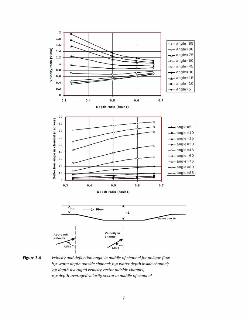
Based on a numerical solution of this set of equations, Delft Hydraulics has presented design graphs for the

current velocity vector v=(ux2+uy

2)0.5 and deflection angle in the middle of a channel oblique to the flow (Figure

3.4). The water depth outside the channel is in the range between 2.5 and 10 m. The channel depth with respect

to the surrounding bottom is 5 m. The side slopes of the channels are 1 to 10. The bottom width is 200 m. The

approach velocity is 2 m/s. The bed roughness is ks= 0.1 m.

Figure 3.4 shows that the velocity vector v1>v0 for approach angles < 15o. The velocity vector ratio v1/vo can be reasonably well (error of 10% to 20% for approach angles between 10o and

90o) represented by: v1/vo=[(ho/h1)(sino/sin1)].

The deflection angle 1 can be reasonably well (error of 10% to 20% for approach angles between 10o and 90o)

represented by: 1= atan[(ho/h1)tan(o)].

7

Figure 3.4 Velocity and deflection angle in middle of channel for oblique flow

h0= water depth outside channel; h1= water depth inside channel;

v0= depth-averaged velocity vector outside channel;

v1= depth-averaged velocity vector in middle of channel

0

0.2

0.4

0.6

0.8

1

1.2

1.4

1.6

1.8

2

0.3 0.4 0.5 0.6 0.7

Depth ratio (ho/h1)

Ve

loc

ity

ra

tio

(v

1/v

o)

angle=85

angle=80

angle=75

angle=60

angle=45

angle=30

angle=15

angle=10

angle=5

0

10

20

30

40

50

60

70

80

90

0.3 0.4 0.5 0.6 0.7

Depth ratio (ho/h1)

De

fle

cti

on

an

gle

in

ch

an

ne

l (d

eg

ree

s)

angle=5

angle=10

angle=15

angle=30

angle=45

angle=60

angle=75

angle=80

angle=85

h1ho

slopes 1 to 10

Flow

AlfaoAlfa1

Approach

Velocity

Velocity in

channel

8

3.2 Waves

Waves are important for the sediment transport processes due to the stirring action of the orbital fluid motions on the sediment particles. This effect is most pronounced in shallow depths where the wave motion feels the seabottom. Wave motion in the nearshore zone is influenced by refraction, diffraction, shoaling and energy dissipation by wave breaking and bottom friction. Wave breaking in the nearshore zone may result into the generation of additional currents. Wave breaking outside the channel results in a wave-induced set-up on both sides of the channel generating a flow towardss the channel. Due to the presence of the coast the flow in the channel will be deflected in offshore direction (similar to rip currents, see Figure 3.5). Three situations of wave propagation over the channel are herein distinguished:

A. Main channel axis parallel to waves

When the waves are propagating parallel to the main axis of the channel, the wave height in the channel will be reduced somewhat due to the increased water depth. The wave celerity will increase in the channel yielding curved wave crests. Wave energy on the side slopes will be reduced by diffractional effects. Waves with a very small approach angle entering the channel will be refracted out of the area, see Figure 3.5 resulting in reduced wave heights in the channel area near the shore. Furthermore, diffractional effects will occur in the channel for waves running parallel to the channel axis due to differences in depth inside and outside the channel resulting in phase differences and eventually the waves will break up into waves with individual crests inside and outside the channel and the average wave height will be reduced considerably (up to about 40% ; Zwamborn and Grieve, 1964).

B. Main channel axis perpendicular to waves

When the waves are propagating perpendicular to the main axis of the channel, the wave height in the channel

will reduce due to the increased depth. Secondary effects are reflection phenomena at the edges of the side

slopes.

C. Main channel axis oblique waves

When the waves are propagating oblique to the main axis of the channel, shoaling and refraction effects will occur and a rather disturbed wave patttern may be generated in the channel depending on the depth and wave approach angle. In case of a relatively small approach angle, the incoming waves may be trapped (refracted/reflected backwards) on the slope of the deepened area resulting in a significantly smaller wave height in the channel, see Figure 3.5. A cross wave pattern consisting of incoming and outgoing waves will be generated outside the channel. The critical wave approach angle (with respect to the channel axis) is about 25o to 30o for a depth of 15 to 20 m, side slopes of 1 to 7 and channel depth of 5 to 10 m. Incoming waves with an approach angle larger than the critical value will cross the channel; the wave direction of the waves leaving the channel will more or less the same as that of the incoming waves due to compensating refractional effects on both side slopes (in case of a relatively narrow channel, Fig. 3.5). Large vessels require longer, deeper and wider approach channels. These channels cause considerable changes in the wave field due to refaction and diffraction which affect the wave conditions in the channel. Wave trapping will occur for waves making a small critical angle (about 25o) with the channel axis resulting in concentration of relatively large waves in the harbour entrance area during storm events (see Figure 3.6). Wave trapping implies that the waves will refract just enough to remain on the side slopes of the channel causing a large increase in wave height until a state of instability is reached and the waves move sideway across the channel. Based on laboratory scale tests with longcrested regular waves, Zwamborn and Grieve (1974) report a wave height increase up to 30% with respect to the incident wave height on a channel slope of 1 to 20. This may cause damage to the breakwater heads and may lead to severe sedimentation in the harbour entrance area and scour in front of the breakwater heads.

9

Figure 3.5 Effect of channel on wave propagation

Waves with an angle larger than the critical angle (>25o) will just pass the channel and waves with an angle smaller than the critical angle will be refracted away from the channel leading to reduced wave heights in the entrance area. Wave trapping effects on the side slope will only occur for a small wave direction sector, but it may lead to serious problems if this direction is close to the dominant wave direction. The problems can be solved by reducing the side slope of the channel facing the critical wave direction. Zwamborn and Grieve (1974) found that the wave trapping effect could be reduced significantly by the following measures:

• side slope of 1 to 100 (instead of 1 to 20), but this will lead to a relatively large increase of the capital dredging;

• V-shape of the channel cross-section to refract the wave energy to the channel slope from where the wave energy can move out of the channel;

• short breakwater running parallel to the channel axis over a short distance (about 100 m). Laboratory tests with directional irregular waves showed, however, that the wave trapping and wave concentration phenomena are much less critical than in tests with longcrested regular waves. The measured wave heights in the entrance area was significantly larger in the test series with regular waves.

Crossing waves

Reflecting waves

Waves refracting

from channel

COAST

Channel

cr. angle

Wave breaking

Offshore

currents

10

Figure 3.6 Wave trapping at channel slope resulting wave height increase in harbour entrance area 4. Mathematical description and simplifications

4.1 Introduction The most general description of the transport processes and associated morphological bed evolution (deposition, erosion and migration) can be obtained by a three-dimensional approach based on numerical solution of the advection-diffusion equation, which reads as (Van Rijn, 1993, 2012; Lesser, 2000):

c/t+(uc)/x+(vc)/y+((w-ws)c)/z-(s,xc/x)/x-(s,yc/y)/y-(s,zc/z)/z=0 (4.1) with: c=suspended sediment concentration, u,v,w= fluid velocities in x, y and z-directions, z= vertical direction,

ws= settling velocity, s,x, s,y, s,z= sediment mixing coefficients in x, y and z-directions. The depth-integrated (from the top of the bed-load layer to the water surface) suspended transport rates in x and y-directions are defined by:

qs,x=(uc-s,xc/x)dz and qs,y=(vc-s,yc/y)dz (4.2) The bed level evolution follows from:

zb/t + [(1-p)s]-1 [(qt,x)/x+(qt,y)/y]/ =0 (4.3)

with zb= bed level to horizontal reference plane, s= sediment density, p= porosity of bed material, qt,x=total depth-integrated sediment transport (bed load plus suspended load transport, in kg/s/m) in x-direction, qt,y= total depth-integrated sediment transport (bed load plus suspended load transport, in kg/s/m) in y-direction. These equations can be solved for given flow velocities, sediment mixing coefficients, settling velocity, sediment concentrations at all boundaries and at initial time (t=0).

Simple engineering methods are available for schematized conditions. Herein, two methods are presented.

Channel

Waves

Slope

Entrance

11

4.2 Simple engineering rules for channels perpendicular, oblique or parallel to flow

4.2.1 Volume of cut method The dredging volumes in the proposed channel layouts can be roughly estimated by a simple “rule of thumb”, known as the “volume of cut” method (Trawle and Herbich, 1980; Van Rijn, 2006, 2012). The deposition in the channel is related to the volume of cut, which is the volume of material required to be removed beyond the natural depth to achieve the desired channel dimensions fo a given channel reach. The formula reads as:

Vd= Vcut

with: Vd= deposition volume of channel section considered and Vcut= volume of cut below natural bed, = proportionality factor. Trawle and Herbich showed that this method can be used to determine the increase of maintenance dredging volume due to the enlargement of a channel (increase of volume of cut). They compared channel sedimentation values (dredging volumes) for the old and the new situation. The new situation refers to the channel enlargement (wider, deeper and/or longer channel). The maintenance dredging volumes (per year) and the volumes of cut for the enlarged channel and for the old channel were compared and expressed as a percentage of increase (Vnew-Vold/Voldx100%). Data from six harbour sites in the USA are given in Table 4.1. Information of the sediments at these sites is not given, but most channels are situated in fine sandy offshore conditions (0.1 to 0.3 mm sand). The percentage of increase of the maintenance dredging volume (Idredge) is roughly equal to the percentage of increase of the volume of cut (Icut), confirming the validity of this method. Thus, the maintenace dredging volume (Vmd) in the new situation due to channel enlargement can be determined from the maintenance dredging volume in the old situation and the increase of the volume of cut, as:

Vnew, md= Vold, md + Icut Vold,md with: Icut = (Vnew,cut-Vold,cut)/Vold,cut

Except for the Yaquina site, the -values are in the range of 0.07 to 0.18 with an average value of:

= 0.120.06 (variation of 50%). This means that the maintenance dredging volume per year for an offshore channel between the port and deep water (at 10 to 12 m depth contour) is approximately equal to 10% of the volume of cut.

The -value for the Yaquina site is considerably larger (about 0.25 to 0.30), which may related to the type of sediments (unknown) and the type of channel (interior channel; over 70% of length inside Bay). Data of some other approach channels are given in Tables 4.1 and 4.2.

The -value of the offshore EURO-MAAS Channel to the Port of Rotterdam (Netherlands) is about 4% (dredging volume of about 1.6 million m3/year, consisting of mud, silt and fine sand; tidal currents of 0.5 to 0.7 m/s; wave heights up to 5 m).

The -value for the sedimentation of mud and silt in the offshore navigation channel to the Port of Bintulu, Indonesia varies between 7% and 10%. The sea bed mainly consists of soft mud. The tidal range is about 1 m. The flood velocities crossing the channel are in the range of 0.1 to 0.15 m/s and the ebb velocities are in the range of 0.05 to 0.1 m/s.

12

Harbour site Channel length old (m)

Channel length new (m)

Channel width old (m)

Channel width new (m)

Water depth in channel old (m)

Water depth in channel new (m)

Wilmington, Atlantic ocean (offshore channel, partly in lee of headland)

8200 8800 120 150 10.5 12.1

Pascagoula, Gulf of Mexico (offshore channel)

6700 8500 100 105 11.5 12.1

Calcasieu, Gulf of Mexico (offshore channel)

21000 38000 75 120 11.2 12.7

Sabine-Neches, Gulf of Mexico (offshore channel, over about 30% of length between jetties)

12500 34000 240 240 11.2 12.7

Galveston, Gulf of Mexico (offshore channel, over about 50% of length between jetties)

14000 16000 240 240 11.5 12.7

Yaquina, Pacific Ocean (mainly interior channel in Bay)

5200 5500 90 120 7.9 12.1

Harbour site

Vcut old (106 m3)

Vcut new (106 m3)

Vdredge old (106 m3)

Vdredge new (106 m3)

I cut

(%)

I dredge

(%)

Acut old (m2)

Acut new (m2)

Ad old (m2)

Ad new (m2)

Wilmington

3.2 5.9 0.41 0.65 60 85 390 670 50 74

Pascagoula 2.9 3.5 0.3 0.51 25 45 430 410 45 60

Calcasieu 7.0 24.3 0.98 4.4 350 250 330 640 47 115

Sabine-Neches

12.1 26.2 1.81 3.8 105 115 970 770 145 110

Galveston 11.5 21.5 0.85 1.5 70 80 820 1340 60 80

Yaquina 0.53 2.3 0.16 0.6 270 370 100 420 30 110

Vcut = volume of cut below natural bed of channel section considered Vdredge = volume of maintenance dredging per year Icut=[volume of cut (new)-volume of cut (old)]/ volume of cut (old)x100% Idredge=[volume of dredge (new)-volume of dredge (old)]/ volume of dredge (old)x100% Acut = volume of cut/channel length= average area of cut below natural bed Ad = volume of dredge/channel length= average sedimentation area in channel Table 4.1 Dredging volumes in USA Channels (Trawle and Herbich, 1980)

13

Harbour site Depth outside channel (m)

Channel depth below bed (m)

Channel width, bottom, top (m)

Channel length (m)

Vcut (106 m3)

Vdredge or Vd (106 m3)

(-)

Type of sedi ment

Rotterdam Port EURO-MAAS Channel

15 to 20 12 to 7 600 1000

5000 38 1.6 0.04 mud, silt, fine sand

Bintulu Port Channel M2

11 4.5 240 330

2000 3 0.2 0.07 mud, silt

Bintulu Port Channel M1+M7

7 8.75 610 785

2500 16 1.6 0.10 mud, silt

Mangalore Port Section BB 1975

8.5 2 200 400

1000 0.6 0.5 0.8 mud, silt

Mangalore Port Section BB 1984-1990

8.5 5.3 200 420

1000 1.65 1.0 0.6 mud, silt

Mangalore Port Section BB 1990-1997

8.5 7 240 450

1000 2.4 1.0 0.4 mud, silt

Suez Canal Channel, zone 2

10 7 250 500

3000 7.9 2.1 0.27 mud, silt

Suez Canal Channel, zone 3

12 to 14 5 400 700

3500 9.6 2.5 0.26 mud, silt

Suez Canal Channel, zone 4

14 to 17 4 450 1100

6500 21.5 1.6 0.08 mud, silt

Damietta channel, Egypt

6 to 12 9 to 3 250 (mean)

4000 6 0.8 0.13 silt, fine sand

Port of Santander channel

9 3 100 300

1500 0.9 0.2 0.2 fine sand

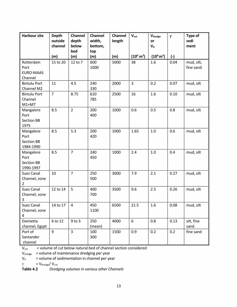
Vcut = volume of cut below natural bed of channel section considered Vdredge = volume of maintenance dredging per year Vd = volume of sedimentation in channel per year

= Vdredge/ Vcut Table 4.2 Dredging volumes in various other Channels

14

The -value for the sedimentation of mud and silt in the offshore navigation channel to the Port of New Mangalore, India varies between 40% and 80%, see Table 4.2. The sediment concentrations in the Mangalore area are relatively large during the monsoon period (wave stirring effect), resulting in rather large sedimentation

values (large -values).

The -value for the sedimentation of mud and silt in the offshore navigation channel to the Suez Canal (near Port

Said) in Egypt varies between 8% and 27%; the -value is smallest in the most offshore zone. The bed material consists of silty sediments in the range of 0.01 to 0.03 mm. The tidal range is not more than about 0.2 m. The flow pattern is mainly wind-driven (0.1 m/s in summer and 0.4 m/s in winter). Deep water waves are larger than 3 m for about 5% of the time (winter storms).

The -value for the sedimentation of fine sand and silt in the inlet channel to the Port of Damietta (Egypt) situated along the Nile-delta coast facing the Mediterranean Sea is about 13%, see Table 4.2. The bed material near the channel consists of sandy sediments of about 0.08 to 0.2 mm. The tidal range is about 0.2 m. The maximum wave height is about 4 m at a depth of 12 m. The maximum longshore currents inside and outside the surf zone are about 0.5 m/s on both sides of the channel. The littoral drift is estimated to be about 0.5 106 m3/yr on both sides of the breakwaters.

The -value for the sedimentation of fine sand in the inlet channel to the Port of Santander (Spain) is about 20%, see Table 4.2. The bed material consists of sandy sediments of about 0.25 mm. The tidal range varies between 1.5 and 3 m (neap-spring). The peak tidal flows are bout 1 m/s. Based on all information, the deposition volume of a dredged channel can be estimated to be about:

• 25% to 75% of the capital dredging volume in muddy inland conditions,

• 10% to 15% of the capital dredging volume in silty/sandy nearshore conditions,

• 5% to 10% of the capital dredging volume in silty/sandy offshore conditions. 4.2.2 SED-PIT model An EXCEL programme (SED-PIT) based on the trapping efficiency method can be used to compute the deposition in a channel, trench or pit for given flow, wave and sediment characteristics at the upstream boundary (x=0 m), (Van Rijn, 2006, 2012). The channel or pit is schematized (see Figure 4.1) into a rectangular cross-section with width B (normal to main channel axis) and depth

15

Figure 4.1 Definition sketch Schematization of sediment transport across channel Assuming a rectangular cross-section with effective length L (see Figure A.1) and using Qs=bqs (and Qs,o=boqs,o; Qs,1=b1qs,1; o refers to upstream; 1 refers to channel), the reduction of the suspended sediment transport per unit channel length (qs,x) after distance x is: qs,x=(bo/b1)qs,o - [(bo/b1)qs,o - qs,1](1-e-Ax) = (bo/b1)qs,o (e-Ax) + qs,1(1-e-Ax) with: bo= streamtube width of approaching flow; b1= streamtube width in channel, qs,o= suspended transport capacity of approaching flow (per unit channel length), qs,1= suspended transport capacity in channel (per unit channel length), x= coordinate along streamtube, A= coefficient. d=h1-ho=depth below upstream bed level, h1=flow depth in channel, ho=flow depth outside channel, L=length of channel (parallel to main channel axis).

16

This approach has been frequently used to estimate the backfilling of relatively narrow navigation channels and pipeline trenches. The trapezoidal cross-section is schematized to a rectangular cross-section making intersections halfway the side slopes. The effective deposition length is the length between the intersection

points, yielding L= B/(sin1). The empirical coefficients can be improved by use of results from trial dredges or from observed deposition rates in existing channels, trenches or pits. Trapping efficiency according to Eysink-Vermaas (1983) The suspended sediment transport in the channel after distance x is expressed as: qs,x=(bo/b1)qs,o - [(bo/b1)qs,o - qs,1)] [1 - exp(-Aevx/h1)] with: Aev= 0.015(2ws/u*,1) [1+(2ws/u*,1)] [1+4.1(ks/h1)0.25]= coefficient ks= bed roughness, ws= settling velocity, u*= bed-shear velocity.

Using x= B/sin1, the backfilling rate (s) per unit channel length is (see Figure 3.1):

s= [(bo/b1)qs,o - qs,1] [1 - exp(-AevB/(h1sin1))] sin1 Trapping efficiency according to Van Rijn (1987) Van Rijn (1987) has introduced two graphs, which can be used to determine the trapping efficiency of suspended sediments from oblique and cross flows over an infinitely long channel. The graphs are based on simulations using the sophisticated SUTRENCH-model (Van Rijn, 1987). The definition sketch is shown in Figure 4.1. The trapping efficiency (es) is defined as the relative difference of the incoming suspended load transport (qs,o) and the minimum suspended load transport in the channel (qs,1,minimum), as follows: es= (boqs,o-b1qs,1,minimum)/(boqs,o) The basic parameters determining the trapping efficiency of a channel, are: approach velocity (vo), approach angle

(o), approach depth (ho), approach bed-shear velocity (u*,o), particle fall velocity (ws), wave height (Hs), channel

depth (d), channel width (B), channel side slopes (tan) and bed roughness (ks). In all, 300 computations have been made using: - approach velocity vo= 1 m/s and approach water depth ho= 5 m,

- approach angles o = 15o to 90o, - channel depths d= 2 to 10 m, - channel width (normal to axis) B= 50 to 500 m, - particle fall velocity ws= 0.0021 to 0.036 m/s, - bed roughness ks= 0.2 m. The influence of the relative wave height (Hs/h) and relative bed roughness (ks/h) on the trapping efficiency (es) is relatively small and has therefore been neglected. The error of the es-parameter is about 25% for an error of the approach velocity of 20% (with Hs/h in the range of 0 to 0.3 and ks/h in the range of 0.02 to 0.06).

17

The trapping efficiency for o = 90o (cross flow) can be roughly represented by:

es= 1-exp(-AvrLd/h12)

es= 0 for very fine sediment if Hs/h1>0.3 for fine sediments (clay, mud) with:

Avr= 0.25[ws/u*,1] [1+(2ws/u*,1)]= coefficient, L= effective settling length, d= h1-ho=channel depth, h1= flow depth in channel,

=1+Hs/h1= enhancement factor related to waves for fine sediment (clay, mud); =1 for silt and sand. If the relative wave height inside the channel is larger than 0.3 (Hs/h1>0.3), it is assumed that very fine sediments cannot be trapped. The trapping efficiency es approaches zero for d approaching zero (no channel).

The sedimentation rate (S) per unit channel length immediately after dredging can be determined from:

S= (es qs,o + eb qb,o) sino with: es= trapping efficiency for suspended load, eb= trapping efficiency (about 1) for bed load, qs,o = incoming suspended load transport per unit channel length, qb,o = incoming bed load transport per unit channel length. SEDPIT-model Three sediment fractions are considered: - clay with settling velocity ws,clay (input value), - silt with settling velocity ws,silt (input value), - sand with settling velocity ws,sand (input value). The parameters L, B, h1 and ho are input values. The width B is determined by the two mid-slope locations (Figure 4.1). The representative tidal period is schematized into 6 blocks of 1 hour for flood and 6 blocks of 1 hour for ebb. Computation over time is established by multiplying with the number of tides (input value; 2 tides per day) considered. The upstream transport rates are defined as: - qs,o,clay= cclay,o vo ho, - qs,o,silt= csilt,o vo ho, - qs,o,sand based on approximation functions, with: vo= tidal flow velocity outside channel (input value in m/s),

ho= flow depth outside channel=hMSL+h, hMSL=water depth to MSL (input value),

h=tidal water level to MSL (input value), co= depth-mean concentration upstream of channel (input values in kg/m3).

18

Calibration factors (input values) can be used to adjust the upstream sand transport.

The deposition S (in kg) per fraction is computed as: s= [(bo/b1)qs,o - qs,1] es t L sin1 with: qs,o= equilibrium sediment transport at upstream boundary based on Van Rijn 2007, 2012, qs,1= (v1/vo)3qs,o=equilibrium transport in channel/pit, bo= width of streamtube at upstream boundary, b1= width of streamtube in channel/pit, es= trapping efficiency according to the methods of Van Rijn (2006, 2012) and Eysink-Vermaas (1983).

The effective deposition length is computed as: Leff= B/sin(1)

The velocity vector v1 is described by: v1 = vo[(ho/h1)(sino/sin1)]

The deflection angle 1 is described by: 1= atan[(ho/h1)tan(o)] The streamtube width in the channel/pit follows from: b1= vohobo/u1h1

The total deposition mass is: Stot= Sclay+Ssilt+Ssand.

The total deposition volume is: Stot, volume= Stot/bulk. The bulk density (ton/m3) is represented by: - constant input value (in range of 0.4 to 1.5 ton/m3); or by

- formula bulk= (Sclay/Stot)(0.415+0.43x0.255) + (Ssilt/Stot)(1.12+0.43x0.09) +(Ssand/Stot)(1.55),

with: = [{(T/(T-1))ln(T)}-1]= consolidation factor (T in years; =0 for period<1 year).

The deposition layer thickness is: hs= Stot, volume/(L B).

The new flow depth in the channel/pit at time t+t is: h1,t+t= h1,t-hs,t; the total deposition thickness can not be larger than the maximum deposition thickness (d= h1-ho). The deposition thickness values should be spread evenly over all tidal blocks, otherwise the number of tides should be reduced. In the latter case the total computation period should be split into several runs.

Example case The SED-PIT model has been applied to determine the sedimentation volume in a trial pipeline trench dredged

in the bed of the Dutch Sector (near harbour of Scheveningen) of the North Sea (sand between 0.2 and 0.3 mm)

in March 1964. The trial trench was dredged perpendicular to the shoreline between 1 km (local depth of about

7 m below MSL) and 1.7 km (local depth of 10.5 m) from the RSP-baseline on the beach. The length of the

trench along the main axis of the trench was about 700 m; the bottom width of the trench was about 10 m; the

side slopes of the trench were about 1 to 7 and the trench depth below the surrounding sea bed was about 2

m. In all, about 30,000 m3 was dredged. The local peak flood and ebb currents are estimated to be in the range

19

of 0.6 to 0.5 m/s parallel to the shoreline (perpendicular to the trench axis). The trench was sounded regularly

in the period between 7 March and 27 August 1964. The measured sedimentation volumes are about 12 m3/m

after 48 days and about 35 m3/m after 173 days (7 March-27 Aug. 1964) at Line 2 with a depth of 8 m (below

MSL), see Figure 4.2.

The input values are, as follows:

Trench: L= 1000 m, B= 20 m (see Figure 3.2), h1= 11 m, d=h1-ho,MSL= 3 m, o= 90o, bo= 1 m,

Sediment: d50= 0.0002 m, d90= 0.0003 m, w= 1020 kg/m3, s= 2650 kg/m3, = 0.000001 m2/s, ws,clay= 0.0001 m/s, ws,silt= 0.001 m/s, ws,sand= 0.018 m/s, cclay,o= 0 kg/m3, csilt,o= 0 kg/m3, ks= 0.05 m, bulk density of sand bed=1550 kg/m3,

Tide: hflood= 0.5 m, hebb= -0.5 m, ho,MSL= 8m vo,flood= 0.3, 0.3, 0.6, 0.6, 0.3, 0.3 m/s, vo,ebb= 0.25, 0.25, 0.5 ,0.5, 0.25, 025 m/s, Waves: Hs= 1 m, Tp= 7 s (representative wave height of 1m over full period),

Sand transport: Calibration factor with =0.5, Total sedimentation period: 173 days or 346 tides (2 tides per day). Based on one run with 346 tides, the computed total sedimentation thickness after 173 days (=346 tides) is: 2.48 m. The computed total sedimentation volume per m is: 49.6 m3/m. The overall trapping efficiency is about 11%. The effect of a clay concentration of 0.05 kg/m3 on the sedimentation volume is marginal (<<1%). A silt concentration of 0.05 kg/m3 results in an increase of 2% of the sedimentation volume. The computed and measured results are shown in Figure 4.3. The computed sedimentation volume is in good agreement with measured values for a calibration factor (on upstream sand transport) of 0.5. Most probably, the representative wave height of 1 m over the full period of 173 days is somewhat too large and hence the computed sand transport rates at the upstream boundary are somewhat too large (using a default calibration factor of 1).

Figure 4.2 Measured bed profiles of trial trench near Scheveningen(North Sea) and schematized cross-section

for SED-PIT mode

-16

-15

-14

-13

-12

-11

-10

-9

-8

-7

-6

0 20 40 60 80 100 120

Cross-shore distance (m)

Dep

th t

o N

AP

(m

)

Line 2; Measured 9 March 1964Line 2; Measured 27 August 1964

South North

20

Figure 4.3 Measured and computed sedimentation volumes for trench near Scheveningen, North Sea The SED-PIT model has also been used to determine the effects of the most important sedimentation parameters on the sedimentation thickness for a channel with depth of 20 m and a depth of 10 m outside the channel. The base case is, as follows:

Trench: L= 1000 m, B= 200 m, h1= 20 m, d=h1-ho,MSL= 10 m, o= 90o, bo= 1 m,

Sediment: d50= 0.0002 m, d90= 0.0003 m, w= 1020 kg/m3, s= 2650 kg/m3, = 0.000001 m2/s, ws,clay= 0.0001 m/s, ws,silt= 0.001 m/s, ws,sand= 0.02 m/s, cclay,o= 0 kg/m3, csilt,o= 0 kg/m3, ks= 0.05 m, bulk density of sand bed=1550 kg/m3,

Tide: hflood= 1 m, hebb= -1 m, ho,MSL= 10 m vo,flood= 0.8 m/s (6 blocks), vo,ebb= 0.8 m/s (6 blocks), Waves: Hs= 0 m, Tp= 7 s,

Sand transport: Calibration factor =1.0, Total sedimentation period: 30 days or 60 tides (2 tides per day). The approach velocity has been varied in the range of 0.6 to 1 m/s. The results are shown in Figure 4.4. The approach velocity has a large effect on the incoming sand transport and hence on the sedimentation layer thickness.

0

5

10

15

20

25

30

35

40

45

50

0 50 100 150 200

Number of days

Sed

imen

tati

on

vo

lum

e (

m3)

Measured sed. volume

Computed sed. volume (calibration factor sand tr.=1.0)

Computed sed. Volume (calibration factor sand tr.=0.5)

21

Figure 4.4 Effect of approach velocity on sedimentation layer thickness

Figure 4.5 Effect of wave height on sedimentation layer thickness

Figure 4.6 Effect of fall velocity on sedimentation layer thickness

0

1

2

3

4

5

6

0 5 10 15 20 25

Sed

imen

tati

on

th

ickn

ess

(m/m

on

th)

Channel/pit depth (m)

Approach velocity= 0.6 m/s

Approach velocity= 0.8 m/s

Approach velocity= 1 m/s

0

3

6

9

12

15

0 5 10 15 20 25

Sed

imen

tati

on

th

ickn

ess

(m/m

on

th)

Channel/pit depth (m)

Hs= 0 m

Hs= 1 m

Hs= 2 m

Hs= 3 m

0

0.4

0.8

1.2

1.6

2

0 5 10 15 20 25

Sed

imen

tati

on

th

ickn

ess

(m/m

on

th)

Channel/pit depth (m)

Fall velocity Ws=0.015 m/s

Fall velocity Ws= 0.02 m/s

Fall velocity Ws=0.025 m/s

22

Figure 4.7 Effect of channel width on sedimentation volume and layer thickness

Figure 4.8 Effect of flow approach angle on sedimentation layer thickness The significant wave height has been varied in the range of 0 to 3 m (peak wave period of 7 s.). The results are shown in Figure 4.5. The wave height has a large effect on the incoming sand transport and hence on the sedimentation thickness in the channel. The fall velocity has been varied in the range of 0.015 to 0.025 m/s (see Figure 4.6). The fall velocity has a minor effect on the sedimentation process for channel depths < 10 m and almost no effect for depths>10 m. The channel width has been varied in the range of 150 to 250 m. The effects on the sedimentation volume and thickness are shown in Figure 4.7. The sedimentation volume increases with increasing channel width due to the

0

0.5

1

1.5

2

2.5

3

3.5

4

0

50

100

150

200

250

300

350

400

0 5 10 15 20 25

Sed

imen

tati

on

th

ickn

ess (

m/m

on

th)

Sed

imen

tati

on

vo

lum

e (

m3/m

/mo

nth

)

Channel/pit depth (m)

Width= 150 m

Width= 200 m

Width= 250 m

Sedimentation volume

Sedimentation thickness

0

0.2

0.4

0.6

0.8

1

1.2

1.4

1.6

1.8

2

0 5 10 15 20 25

Se

dim

en

tati

on

th

ick

ne

ss

(m

/mo

nth

)

Channel/pit depth (m)

Angle= 90

Angle= 70

Angle= 50

Angle= 30

Angle= 10

23

increase of the trapping efficiency. The sedimentation thickness decreases with increasing channel width, because the increase of the trapping efficiency is less effective than the increase of the width. The flow approach angle has been varied in the range of 90 to 10 degrees. The results are shown in Figure 4.8. The sedimentation thickness is maximum for a flow approach angle of 90 degrees and decreases with decreasing flow approach angle due to the effect of increasing velocities in the channel (flow refraction effect). Based on this, it is favourable to align the channel axis as much as possible with the flow direction. Cross flows should be avoided as much as possible. 4.3 Effect of flow approach angle on deposition The computed deposition strongly depends on the angle between the main tidal flow and the channel axis in each channel section. In most channel sections this angle is small (< 5o), but its exact value is not very well known as detailed flow measurements or numerical flow model computations are not available. When the flow vector crosses the channel, the flow vector is refracted at the upstream slope of the channel resulting in a smaller angle between the flow vector and the axis. At the downstream slope, the flow vector is refracted back to its orignal direction in the case of a symmetrical channel cross-section. When the tidal flow is fully parallel to the channel axis, the flow velocities increase due to reduced bed friction (larger depth). As a result, the mud deposition may reduce to zero. The channel bed may even be eroded slightly due to increasing flow velocities (larger depth and thus reduced bed friction). 4.3.1 SEDPIT-model The SEDPIT-model has been used to compute the deposition volumes in a schematic channel section for flow approach angles in the range of 1o (almost parallel flow) to 90o (cross-flow). The flow assumed to be is stationnary (no tidal flow). The water depth outside the channel is 9 m. The channel depth below the surrounding bed is 3 m. The channel width is 155 m. The approach flow velocity is 1 m/s. The upstream mud concentration is 300 mg/l. The mud settling velocity is 0.7 mm/s. The bed roughness is 5 mm. The dry bulk density is 600 kg/m³. The results are plotted in Figure 4.3.1. The deposition is maximum for cross flow and 0 for parallel flow, see Table 4.3.1. As the SEDPIT-model is a simplified model which cannot compute the deposition volume with sufficient accuracy for small angles, the DELFT2DH/3D-model has also been used. The results of the DELFT2DH/3D-models (see Section 3.5.2) are also shown in Table 4.3.1. Figure 4.3.1 shows the relative deposition D/D90, with D90=deposition in channel for approach angle of 90o, producing the highest deposition volume. The DELFT-model yields much smaller deposition rates for small approach angles than the SEDPIT-model. The flow velocities in the channel computed by the DELFT-model are relatively high (reduced friction due to larger depth) compared to those of the SEDPIT-model. The SEDPIT-model underestimates the velocities in the channel resulting in more deposition (upper estimate).

24

Case Approach angle

Deposition SEDPIT-model (m3/month)

Deposition DELFT2DH-model (m3/month)

Deposition DELFT3D-model (m3/month)

0o 0 16500 9500

1o 33300

3o 45500

5o 49000 20700 13800

10o 52800 25800 18000

15o 57000 30600 23000

20o 60000

30o 68500 48000 54300

40o 79000

50o 90000

60o 100000 115000 142400

70o 107000

80o 112000

90o 114000 152500 189200

Table 4.3.1 Computed deposition volumes

Water depth to MSL= 9 m; channel width= 155 m; channel depth = 3 m; approach velocity = 1 m/s, cmud= 300 mg/l; ws,mud=0.7 mm/s; dry bulk density= 600 kg/m3; bed roughness ks= 5 mm Figure 4.3.1 Effect of flow approach angle on dimensionless deposition in schematic channel section

D= mud deposition volume in channel at angle ; D90= deposition in channel at angle=90o

0

0.1

0.2

0.3

0.4

0.5

0.6

0.7

0.8

0.9

1

0 5 10 15 20 25 30 35 40 45 50 55 60 65 70 75 80 85 90

Dim

en

sio

nle

ss d

ep

osit

ion

D/D

90

Angle between tidal flow vector and channel axis (degrees)

SEDPIT-model

DELFT2DH-model

DELFT3D-model

Channel

Approach angle

Flow vector

25

4.3.2 DELFT2DH/3D-model Similar computations have been made using the DELFT2DH-model and the DELFT3D-model (10 layers). The channel length is 2000 m. The channel width is 150 m at the bottom and 160 m at the surrounding bed. The other data are similar to those used in the SEDPIT-model. Figures 4.3.2A,B show computed flow velocity patterns and values for stationary flow. The results are:

• angle=0o, 5o, 10o: slight velocity decrease in upstream channel part and increase in downstream part;

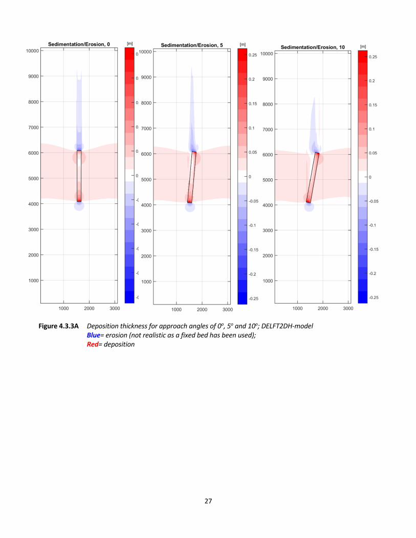
• angle=30o, 60o, 90o: velocity decrease in channel. Figures 4.3.3A,B show computed deposition patterns. The results are:

• angle=0o, 5o, 10o: deposition in upstream and downstream part of channel; less deposition in middle;

• angle=30o, 60o, 90o: deposition in all channel parts. The relative deposition as function of the approach angle is shown in Figure 4.3.1. The computed erosion patterns are not realistic as a fixed bed has been used in the computational domain. The erosion patterns refer to erosion of mud which is deposited at the fixed bed during the numerical startup period. Figure 4.3.2A Flow velocity pattern (depth-averaged) for approach angles of 0o, 5o, 10o; DELFT2DH-model Undisturbed approach velocity= 1 m/s; Blue= velocity <1 m/s; Red= velocity > 1 m/s

Flow velocity= 1 m/s

26

Figure 4.3.2B Flow velocity pattern (depth-averaged) for approach angles 30o, 60o, 90o; DELFT2DH-model Undisturbed approach velocity= 1 m/s; Blue= velocity <1 m/s; Red= velocity > 1 m/s

Flow velocity= 1 m/s

27

Figure 4.3.3A Deposition thickness for approach angles of 0o, 5o and 10o; DELFT2DH-model Blue= erosion (not realistic as a fixed bed has been used); Red= deposition

28

Figure 4.3.3B Deposition thickness for approach angles of 30o, 60o and 90o; DELFT2DH-model Blue= erosion (not realistic as a fixed bed has been used); Red= deposition

29

5. References

Deltares/Delft Hydraulics, 1985. The flow across trenches at oblique angle to the flow. Report S490. Delft Hydraulics, Delft, The Netherlands

Deltares/Delf Hydraulics, 1991. Design of the access channel to Barrow in Furness. Task 5: Detailed currents

and sedimentation. Report H1208. Delft, The Netherlands Eysink, W. and Vermaas, H., 1983. Computational method to estimate the sedimentation in dredged channels

and harbour basins in estuarine environments. Int. Conf. on Coastal and Ports Engineering in Developing Countries, Colombo, Sri Lanka

Lesser, G., 2000. On-line sediment transport within Delft3D-Flow.Report Z3899, Delft Hydraulics, Delft, The Netherlands

Silveira, L. et al., 2017. Integrated method for optimal channel dredging design. Terra et Aqua, No. 146, March

2017 Trawle, M.J. and Herbich, J.B., 1980. Prediction of shoaling rates in offshore navigation channels. Center for

Dredging Studies, Department of Civil Engineering, Texas Engineering Experiment Station, COE report No. 232, USA.

Van Rijn, L.C., 1987. Mathematical modelling of morphological processes in the case of suspended sediment

transport. Doc. Thesis, Delft University of Technology, Delft, The Netherlands Van Rijn, L.C., 1990, 2011. Principles of fluid flow and surface waves in rivers, estuaries, seas and oceans. Aqua

Publications, The Netherlands (www.aquapublications.nl) Van Rijn, L.C., 1993, 2012. Principles of sediment transport in rivers, estuaries, seas and oceans. Aqua

Publications, The Netherlands (www.aquapublications.nl

Van Rijn, L.C., 2007. Unified view of sediment transport by currents and waves, I, II, III. ASCE, Journal of

Hydraulic Engineering, Vol. 133, No. 6, 649-667, 668-689, No. 7, 761-775

Van Rijn , L.C., 2006, 2012. Principles of sedimentation and erosion engineering in rivers, estuaries and coastal

seas. www.aquapublications.nl Zwamborn, J.A. and Grieve, G., 1974. Wave attenuation and concentration associated with harbour approach

channels, p. 2068-2085. 14th ICCE, Copenhagen, Denmark