Stochastic programming and natural gasA modelling perspective

Asgeir TomasgardKjetil T. Midthun

Norwegian University of Science and Technology

The Åsgard field

Outline

The natural gas value chain– Background– Different roles– Physics

Why stochastic programming– Flexibility and bottlenecks– Modelling uncertainty

Model examples– A portfolio optimization model

• Stochastic mixed integer

– A capacity booking model• Stochastic complementarity program

Background

EU natural gas directive– Company based sales– Neutral operator and 3rd party

access to transportation network– Standardized markets

Statoil, our industrial partner– Norway’s largest oil and gas

producer– Operates and sells 70% of

Norwegian gas– Norwegian gas covers 14% of

European consumption

Close cooperation with SINTEF:– F. Rømo, M. Fodstad, M. Nowak,

L. HellemoFunded by

– Statoil, Gassco, Research Council

The natural gas value chain and different roles

Physical modelProduction

Gastransportation

Processingplants

Componentmarket

Financialmarket

ContractmarketSpotmarket

Upstreammarket

Gas storage

The physics: Production,Transportation and Processing

Quality and componentsTransportation

– Gas flows as a consequence of pressure difference

– Physical laws

– Steady state

Qualities and components– Different fields have different

production characteristics and different qualities

Natural gas is a multi commodity flow Fields characterized by composition of gas

Gas fraction GCV [MJ/Sm3] Market value [NOK/Sm3]1 Methane(CH4) 37,70613 0,622 Ethane(C2H6) 66,0665 1,163 Propane(C3H8) 93,93543 1,494 I-Butane(iC4) 121,40344 1,975 N-Butane(nC4) 121,79168 1,976 iC5 149,36288 2,447 nC5 149,65554 2,558 nC6 177,55324 3,029 C7 219,353045 3,5110 H2S 23,78435 0,0011 CO2 0 -0,7012 Nitrogen 0 0,00

Handling the gas qualityMotivation for modeling quality and components

– Gross calorific value (GCV) - Contractual characteristics (Min/max)– The CO2-content is critical for corrosion in the pipelines, and is

generally not wanted– H2S is not wanted due to corrosion– Components necessary to give a relevant description of the processing

terminals - extraction of ethane etc.

Kårstø, Rogaland

The model have 12 gas componentsGas quality is primarily a property relevant to the exit terminals in the network.The Gas quality (GCV) is linear in the gas components: Challenge is to model equal relative split for all 12 components in split nodes:

Gas Quality restrictions

{ }∑

∈

⋅=nethanemethanec

ecce molpergcvGCV,...,,

,

Gas quality and components

Figure 2.3 Preprocessing of split-nodes in the model

A

BC

D E

d2

d1

1 2

1 2ij ij

ik ik

c c

c c

f ff f

=

The relative split to the downstream nodes MUST be equal in all the gas fractionsif 20 % of the gas is routed to j then 20% of the Ethane (c1) and Propane (c2) must go to the downstream node j.

i

j k

Experience: Finds good solutions very quickly, but does not confirm optimality rapidly

, ,

, ,

1 ( 1),

, ,

, ,

c ciA g ig

g

cig ig

c

ìgg

c c cig iA iB

g

c c ciA iB ji

j

f S s i c

s NodeCap i g

S i

s f f i c

f f f i c

λ

λ

= ∀

≤ ∀

= ∀

= + ∀

+ = ∀

∑

∑

∑

∑

∑

Split volume to node A

Total volume through node i

Ordered set of type 1

Volume goes either to A or B

Mass balance

Modelling the split

The physics: steady state modelling

Empirical function - Weymouth equation

ZLTGpp

PTEDQ ui

s

s

⋅⋅⋅−

⋅⋅=22

67,22,137

40

45

50

5560

65

70

75

80

70 80 90 100 110 120

Pressure out [bar]

Flow

cap

acity

[MS

m3/

døgn

]

Pi=160 bar

Pi=130 barPi=140 bar

Pi=150 bar

Pi=120 bar

Weymouth equation

80100

120140

160180

200

50

100

1500

50

100

150

200

Pressure inPressure out

Flo

w

ZLTGpp

PTEDQ ui

s

s

⋅⋅⋅−

⋅⋅=22

67,22,137

ui pPUPI

PUkpPUPI

PIkQ2222 −

−−

≤

Handling pressure

We do a general series expansion round PI and PU:

( ) ( ) ( ) ( ) ( ) ( )PUpPUPIpQPIpPUPI

pQPUPIQppQ u

ui

iui −⋅

∂∂

+−⋅∂∂

+≤ ,,,,

And this is expressed as a linear restriction:

ui pPUPI

PUkpPUPI

PIkQ2222 −

−−

≤

Quality of approximation depends on:• selection of PI-PU pairs• the number of pairs selected

One restriction will be active for each pipeline

Why stochastic programming?

Uncertainty in the markets

Prices from December 2003 to December 2005 (NOK/Sm3)– Prices provided by Heren Energy Ltd.

Three different market hubs: NBP, Zeebrugge and TTF

0

1

2

3

4

5

6

Dat

e

02/0

1/20

04

05/0

2/20

04

10/0

3/20

04

13/0

4/20

04

17/0

5/20

04

19/0

6/20

04

23/0

7/20

04

26/0

8/20

04

29/0

9/20

04

02/1

1/20

04

06/1

2/20

04

08/0

1/20

05

11/0

2/20

05

17/0

3/20

05

20/0

4/20

05

24/0

5/20

05

27/0

6/20

05

30/0

7/20

05

02/0

9/20

05

06/1

0/20

05

09/1

1/20

05

13/1

2/20

05

TTFZeebruggeNBP

Short term uncertainty in Gas prices

Illustration of prices from September 2004 – a period of two weeks

1

1.1

1.2

1.3

1.4

1.5

1.6

Date

13/09

/2004

14/09

/2004

15/09

/2004

16/09

/2004

17/09

/2004

18/09

/2004

20/09

/2004

21/09

/2004

22/09

/2004

23/09

/2004

24/09

/2004

TTFZeebruggeNBP

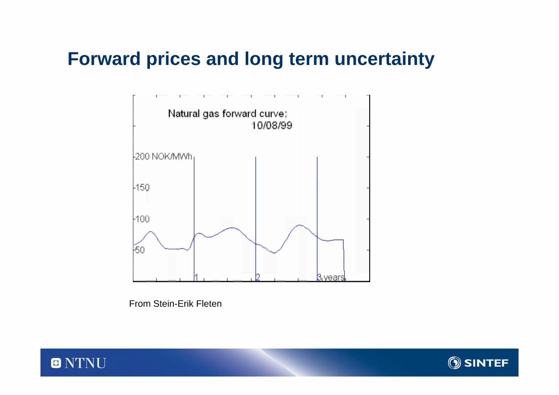
Forward prices and long term uncertainty

From Stein-Erik Fleten

Example on price model for the short runWhen constructing our price model we focus on the winterseason– High seasonality in the price data– Largest variation in prices in the winter season

We remove outliers from the model– Defined as large deviation from the average value in the the week

before and after the observation

We then construct Autoregressive Models of order 2 (AR(2))

Scenario generation

The residuals from the price model is used to createscenarios– We find the first four moments of the residual distribution– We then use a moment matching algorithm to construct our

scenarios

The AR(2) price model is used on the scenario tree– The value in a given event node is equal to the price predicted by

the price model plus the residual from the scenario generation

Example

0

1

2

3

4

5

6

-10 -8 -6 -4 -2 0

NBP Zeebrugge hd NBP hd Zeebrugge

Modeling of TOP volume

Large customerCan not buy all needed gas in the spot marketAssume that demand in customers portfolio is correlated with the spot price

Smaller customerIf spot price is higher than TOP – takes maximum deliveryIf it is lower than TOP – takes minimum delivery

40 %

110 %

PTOP = PSpot Spotprice

40 %

110 %

PTOP=PSpot

Flexibility: Modelling system effects of the pressure

2 alternative model choices– Node pressure

• The pressure is equal on the outlet side of all pipelines going into a junction node in the network

• And the inlet pressure on all outgoing pipelines is also equal to this

• Non-convex feasible region

– More advanced junction nodes with valves

• The inlet pressure on all outgoing pipelines is lower than the smallest outlet pressure on incoming pipelines

• Convex feasible region

Of course in nodes with compressors, the pressure may be lifted

Flexibility and bottlenecks – system effects

Assume we would like to increase flow AE to 41

Supply functions: Demand functions:Node A: cA = qA Node D: pE = 200 – 2 qD

Node B: cB = 3qB Node E: pF = 200 – 3 qE

Using the pipelines as storage:Flexibility and bottlenecks- storage

Use of storage in pipelines

Sell when price is high, build storage when price is low

Example I: Portfolio optimization

The producers perspective

Strategic (3-20 years)Field and pipeline investmentsLong term contractsProduction profilesLifting agreements

Time Horizon 1-7 daysShort term production plans based on market possibilities, transportation capacity, contractsMarket balancing (mixing physical production, spot trades and bilateral trades) Transportation booking (secondary market)Storage utilization

years months Weeks / days

Operational planningmodel output

Tactical (1 m -3 y)Production plansTransportation plans and bookingBilateral contracts, forward and spot allocationStorage profiles

Decision space for a single production field

Time

Vol

ume

Forward contract, spot contract, bilteral contractUpper and lower limits for lifting gas from the fieldForecasted demand for bilateral conracts

Actual demand faced in scenario s for the bilateral contracts

Liberalized market

Field A

Emden

Field B supplies Emden

Field B

Zeebrugge

Field A supplies EmdenField B sells spot in Zeebrugge

Buy spot in EmdenField B sells spot in Zeebrugge

Geographical swaps

Buy spot in EmdenField B sells spot upstream

Supply Emden from storageField B sells spot somewhere

Field B needs to produceBilateral contract in Emden

Liberalized market - time swaps

Field A

Emden

Field B

Zeebrugge

Field B needs to produce in period 1, Bilateral contract in Emden in period 2

Field A

Emden

Field B

Zeebrugge

Field B supplies Storage Storage supplies EmdenField B sells spot in Zeebrugge Buy spot in Emden

T=1 T=2

Production, trading and risk managementTraditional production planning (first level)

– Balancing of production portfolio with contract portfolio

Production and market optimization (second level)– Moving gas in time or geographically– Using forwards or options (or in case of efficient spot market futures or

spot)– Purpose is to maximize profit from production and contract obligations

Trading (third level)– Trade contracts and financial instruments independently from production

and contract obligations

Risk management– Integrated with production planning and trading– Separate risk management

• Can production portfolio and market give you hedges or possibilities that markets cannot give you?

• Differences between a price maker and a price taker?

Two stage tactical modelFirst stage decision variables– short term spot and contract

allocation (monthly)– short term /long term storage– long term bilateral contracts– production allocation– transportation planning

• short and long term contract

– capacity booking– uncertain prices and volumes

Second stage – secondary transportation market– production allocation– transportation planning– spot sales and contracts

36 monthsT=0

T=1

T=2

T=3

Uncertainty and decision flexibility

Modelling uncertainty is important– To calculate the expected value– To model decision flexibility and option values– To find the risk profile you want on your portfolio– Handle forward markets

Deterministic models will– choose sub optimal solutions– choose static solutions– disregard flexibility– have no attitude towards risk

Typical model sizesMonthly model

– Order of a few hundred scenarios (would like more…)– 2 stages– 120.000constraints– 82.000 variables– 640 sos

– Solution time: 10-20 hours

Weekly model:– Order of 4000 scenarios– 3 stages– 1 million constraints, 100000 variables– Solves relatively fast (minutes)– What do we expect from the model?

• Hope to achieve on average a higher price than in the deterministic model• Find the effect of better utilization of the pipeline flexibility• 1% better price on average (in the spot market) will correspond to an added income of 40 mill euro per

year• 1 % added volume corresponds to 150 mill euro per year

Example II:

Equilibrium with several producers and a system operator

Transportation network with a neutral system operator

Field 1 Field 2 Field 3

Market 1 Market 3Market 2

J1 J2

• Price takers in the spot market for gas• Imperfect competition in the transport network

Field 1 Field 2 Field 3

Market 1 Market 3Market 2

Transportationnetwork

Several large producers and a competitive fringe in each fieldPrice takers in the spot market for gasA competitive fringe in the transport networkImperfect competition between large producers in in the transport network

Time and decision structure

Alternative 1:– Large producers make booking decisions and contingent production decisions at

time 0. – This means that production decisions depend on stochastic outcome, but not on

other players booking or production decisions!– Each players problem is a two-stage stochastic program– The problem is in equilibrium when all the players KKT conditions are satisfied

simultaneously.– The resulting problem is a Stochastic complementarity program

Alternative 2:– A large producer first make booking decisions, then observe outcomes AND other

players booking decisions.– Each players problem is a stochastic program with equilibrium constraints (the KKT

conditions from the second stage)– This resulting total problem is a stochastic EPEC– Each players problem is highly non-convex

The decision structure

The complementarity program

Large producer nTime 0

– Booking capacity– Price in spot market is

unknown– (contingent production and

capacity decisions)–

Time 1– Price in spot market is

known– Production decison

imlemented– Sell surplus capacity– Buy addtional capacity

KKT- conditions for n two-stagestochastic programs (now or never)

ISOTime 0

– No decision

Time 1– Routing decision– Sell spare capacity

KKT - conditions for s deterministicoptimization problems (this is a wait and seeproblem)

Competitive fringeTime 0

– No decision

Time 1– Production decision– Buy capacity from ISO

and/or large producers

KKT - conditions for s deterministic optimizationproblems (this is a wait and see problem)

– Existence and uniqueness of solution: • As for Nash equilibrium or Generalized Nash equilibrium

– (Variational inequalities or quasi variational inequalities)

– Solve using AMPL and Path for a Nash-equilibrium– Handles hundreds of scenarios and tens of players– Solution times: minutes to hours

– Intro : http://www.ampl.com/NEW/complement.html

Related work

Klaus Ehrhardt, Marc C. Steinbach. KKT Systems in Operative Planning for Gas Distribution Networks. PAMM, 4(1):606-607, 2004.

Klaus Ehrhardt, Marc C. Steinbach. Nonlinear Optimization in Gas Networks. Modeling, Simulation and Optimization of Complex Processes, p. 139-148, 2005.

Van der Hoeven, T. (2004) Math in Gas and the art of linearization, Ph.D thesis Energy Delta Institute, 10th March 2004, International business school and research centre for natural gas, Groningen, The Netherlands.

Wolf, D. and Smeers, Y. (2000) The Gas Transmission Problem Solved by an Extension of the Simplex Algorithm, Management Science, Vol. 46, No 11, pp 1454-1465.

Martin, Alexander; Möller, Markus; Moritz, Susanne Mixed integer models for the stationary case of gas network optimization. Math. Program. 105 (2006), no. 2-3, Ser. B, 563--582.

Selot, A, Kuok, L.K, Robinson, M., Mason, T.L., Barton, P., , A short-term operational planning model for upstream natural gas production systems, to appear in AiChE journal.

Westphalen, M., Anwendungen der Stochastischen Optimierung im Stromhandel und Gas Transport, PhD thesis, Unvierity Duisburg-Essen, Germany, 2004.

Available papers:

– Dahl, H.J., Rømo, F. and Tomasgard, A. (2003) An optimisation model for rationing-efficient allocation of capacity in a natural gas transportation network, Conference proceedings: IAEE Praha, June, 2003.

– A. Tomasgard, F. Rømo, M. Fodstad, K. Midthun, , Optimization models for liberalized natural has markets, in G. Hasle, K.-A. Lie, E. Quak (editors), Geometric Modelling, Numerical Simulation, and Optimization: Applied Mathematics at SINTEF, Springer, 2007.

– Nowak, M. and Westphalen, M. (2003) A linear model for transient gas flow, Proceedings of ECOS 2003 Vol III, 1751-1758.

Available in August (included in Kjetil Midthun’s PhD thesis): – K. Midthun, A. Tomasgard, M. Bjørndal, Y. Smeers :Capacity booking in a Transportation Network with

Stochastic Demand and a Secondary Market for Transportation Capacity

– Mette Bjørndal, Kjetil Midthun, Asgeir Tomasgard: Modeling optimal economic dispatch and flow externalities in natural gas networks

– K. Midthun, M. Nowak, A. Tomasgard: An operational portfolio optimization model for a natural gas producer

Ongoing work:– L. Hellemo, F. Rømo, A. Tomasgard, M. Nowak, M. Fodstad :An Optimization System Using Steady State

Model for Optimal Gas Transportation on the Norwegian Continental Shelf

– Long-term infrastructure planning /decision dependent uncertainty: with P. Barton , E Armagan (MIT) and L. Hellemo, NTNU

Post doc positions available!Asgeir.tomasgard@iot.ntnu.no