ASEN6517 Computational Methods in

Dynamics (Spring 2014)

Lecture 8: Analysis of Wave Propaga-tion in Solids

8.1 Why study wave propagation algorithms?

There are three categories of dynamics problems:

1. Vibration problems which focus on the resonant frequenciesand their vibration mode shapes (eigenvalues and eigenvec-tors);

2. Transient response analysis of structural, fluid and thermalsystems which are characterized by low-frequency responsecomponents;

3. Wave propagation which is dominated by high-frequencyresponse components and often characterized by discontin-uous response fields such as stress and/or velocity discon-tinuity.

As for the vibration analysis, there are a host of eigenvaluepackages available (see, e.g., http://www.netlib.org/linpack/). Asfor transient analysis of mechanical systems, perhaps, the mostwidely used method for structural dynamics problems is theNewmark method ( Newmark, N. M. (1959) A method of com-putation for structural dynamics. Journal of Engineering Me-chanics, ASCE, 85 (EM3) 67-94.) for implicit integration:

un+1 = un + (1− γ)4tun + γ4tun+1

un+1 = un +4tun +1− 2β

21− γ)4t2un + β4t2un+1

(8.1)

and the central difference method for explicit integration:

un+1/2 = un−1/2 +4t un for n ≥ 1

u1/2 = u0 + 124t u0 for n = 0

un+1 = un +4t un+1/2

(8.2)

1

0 10 20 30 40 50 60 70 80 90 100−0.4

−0.2

0

0.2

0.4

0.6

0.8

1

1.2

1.4

Bar Coordinate

VElocity Profile

Box Wave Propagation along Homogeneous Bar(Courant Number = 0.5)

Exact Solution

Solution byCentral DifferenceMethod

Direction of

Wave Front

Fig. 1. Post-shock spurious oscillations of a box wave passing througha homogeneous bar with step size of Cr = c∆t/∆x = 1/2.

The central difference method is used to trace the wave fronts.

In the above equations 4t is the integration step size, and thesubscript refers to the discrete time tn = n4t.

The central difference method(8.2) is also a favorite explicitscheme for wave propagation analysis in solids for homogeneousand uniform regular mesh models. For one-dimensional prob-lems and uniform meshes, the central difference method workswell if the step size is chosen for the so-called Courant number(Cr) to be unity:

Cr = c4tc/4x = 1 (8.3)

where 4x is the mesh length and c is the one-dimensional speedof the sound of the material at hand.

However, for solids with heterogeneous materials and two andthree-dimensional problems, there are two reasons the use ofthe central difference may lead to unacceptable analysis results.First, for heterogeneous solids the wave speeds are different fromone location to another. This means that the integration stepsize 4tc chosen for the stiff materials such that the Courantnumber to be unity, gives rise to the Courant number muchsmaller than unity, which is known to engender spurious oscilla-tions. To see this, let us integrate wave propagation along a barof uniform materials with different Courant number as shown inFigs. 1 and 2.

2

0.01m/sV =

100mm

X

Elastic Stress Waves in one-dimensional bar

Central Difference Method Cr=0.5

Present Time Integration Cr=0.5

Fig. 2. Wave propagation with dispersion due to disparity ofwave speed and the time step size (shown on the left withCr = c∆t/∆x = 1/2) and without dispersion ( shown on the rightwith Cr = c∆t/∆x = 1). The central difference method and a newmethod (which we will describe shortly) are used to trace the wavefronts.

Second, in two or three dimensional solid problems, unlike influid whose waves propagate with uniform volumetric speed,due to different deviatoric and volumetric wave speeds as wellas special waves such as Lamb and Rayleigh waves that prop-agate along the surface of plates or in the solid layers. Whilewave speed differences in transient wave propagation computa-tions by direct time integration methods, it engenders spuriousoscillations due to the mismatch in wave speeds. Specifically,because of the Courant stability limit of all explicit time in-tegration methods, we have the step size mismatch as shownbelow:

For Longitudinal Wave:

∆tL = `max/cL, cL =

√E

ρ(1− ν2), `max = max(`x, `y)

3

(a)

0 0.2 0.4 0.60.70.8 1−1.5

−1

−0.5

0

0.5

x / L

stra

in (s

tress

)

0 0.2 0.4 0.60.70.8 1−0.2

0

0.2

0.4

0.6

0.8

x / L

disp

lace

men

t

0 0.2 0.4 0.60.70.8 1−0.5

0

0.5

1

1.5

x / L

velo

city

0 0.2 0.4 0.60.70.8 1−60

−30

0

30

60

x / L

acce

lera

tion

(b)

0 0.2 0.4 0.60.70.8 1−1.5

−1

−0.5

0

0.5

x / L

stra

in (s

tress

)

0 0.2 0.4 0.60.70.8 1−0.2

0

0.2

0.4

0.6

0.8

x / L

disp

lace

men

t

0 0.2 0.4 0.60.70.8 1−0.5

0

0.5

1

1.5

x / L

velo

city

0 0.2 0.4 0.60.70.8 1−60

−30

0

30

60

x / L

acce

lera

tion

(c)

0 0.2 0.4 0.60.70.8 1−1.5

−1

−0.5

0

0.5

x / L

stra

in (s

tress

)0 0.2 0.4 0.60.70.8 1

−0.2

0

0.2

0.4

0.6

0.8

x / L

disp

lace

men

t

0 0.2 0.4 0.60.70.8 1−0.5

0

0.5

1

1.5

x / L

velo

city

0 0.2 0.4 0.60.70.8 1−60

−30

0

30

60

x / Lac

cele

ratio

n

(d)

Fig. 3. An one-dimensional discontinuous wave propagation problem:(a) scheme of shock loading of an elastic bar, (b) the pushforwardintegration, (c) the pullback integration, (d) the presented time in-tegration with the averaging parameter θ = 0.5. Time step size is∆t = 0.54x/c.

For Shear Wave:

∆tS = `max/cS, cS =√G/ρ, G =

E

2(1 + ν)< E

Hence, we have the following relation:

cL > cS ⇒ ∆tL < ∆tS

In the preceding equations (∆t, E,G, ν, `x, `y) are time step size,Young’s modulus, shear modulus, Poisson’s ratio (ν > 0 exceptsome engineered materials), and (`x, `y) are elemental mesh sizealong the x and y-directions, respectively.

Ideally, if the longitudinal component and shear component areintegrated by different time step sizes, each with its Courantstability limit, the resulting computations would trace the wavefronts as accurately as they can be. It is this observation thathas been exploited in the development of a new method aimedat achieving this stated goal.

4

8.2 Construction of an algorithm for inducing front-shock os-cillations

It is well-known that wave fronts advance one discrete node pereach time step no matter how small the step size is relative tothe ideal time step size, viz., Cr = c∆tc/∆x = 1. It is recalledthat when the step size is less than the ideal one, ∆t < ∆x/c,the coupling term for the j-th equation, forces part of the waveenergy to be allocated at the (j+1)-node. This happens in spiteof the fact that the wave front is impossible to reach from the j-thnode to the (j+1)-node within one step whenever, ∆t < ∆x/c.Thus the coupling terms in effect play the role of artificiallystretching the wave speed to

cartificial = c∆tc∆t

, ∆tc = 4x/c (8.4)

where ∆tc corresponds to the ideal step size that makes theCourant number to be unity.

It is emphasized that this artificially stretched wave speed (cartificial)gives rise to the post-shock spurious oscillations. This observa-tion suggests that if one artificially increase the step size thatis larger than the actual step size, then perhaps the spuriousoscillations may exhibit in front of the discontinuities instead ofbehind the discontinuities. To this end, we explore the followingcombination of extrapolation and interpolation.

First, we begin with the following semi-discrete equations ofmotion

Mw(t) + Kw(t) = f(t), w(0) = w0, w(0) = w0 (8.5)

where (M,K) are the mass and stiffness matrices; (w, f) are thedisplacement and applied force vectors; and, the superscript dotdesignates time differentiation.

Second, assuming that the displacement (w) and the velocity(w) at time t = n∆t are available, we obtain by an extrapolation(or by an explicit integration formula) the displacement at timetn+c = tn + ∆tc as shown in Figure 4.

wn+c = wn + ∆tc wn +

∆t2c2

wn (8.6)

Here, for simplicity, we have employed the standard central dif-ference method.

5

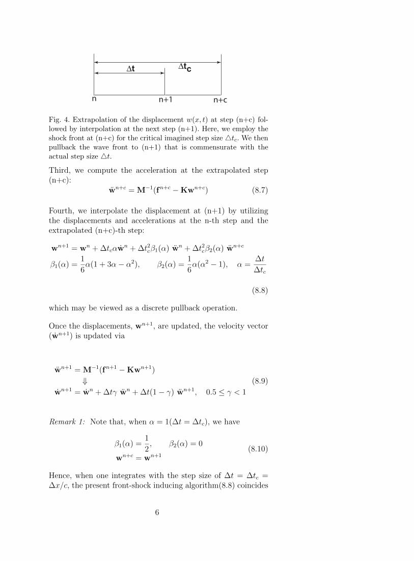
Fig. 4. Extrapolation of the displacement w(x, t) at step (n+c) fol-lowed by interpolation at the next step (n+1). Here, we employ theshock front at (n+c) for the critical imagined step size 4tc. We thenpullback the wave front to (n+1) that is commensurate with theactual step size 4t.

Third, we compute the acceleration at the extrapolated step(n+c):

wn+c = M−1(fn+c −Kwn+c) (8.7)

Fourth, we interpolate the displacement at (n+1) by utilizingthe displacements and accelerations at the n-th step and theextrapolated (n+c)-th step:

wn+1 = wn + ∆tcαwn + ∆t2cβ1(α) wn + ∆t2cβ2(α) wn+c

β1(α) =1

6α(1 + 3α− α2), β2(α) =

1

6α(α2 − 1), α =

∆t

∆tc

(8.8)

which may be viewed as a discrete pullback operation.

Once the displacements, wn+1, are updated, the velocity vector(wn+1) is updated via

wn+1 = M−1(fn+1 −Kwn+1)

⇓wn+1 = wn + ∆tγ wn + ∆t(1− γ) wn+1, 0.5 ≤ γ < 1

(8.9)

Remark 1: Note that, when α = 1(∆t = ∆tc), we have

β1(α) =1

2, β2(α) = 0

wn+c = wn+1(8.10)

Hence, when one integrates with the step size of ∆t = ∆tc =∆x/c, the present front-shock inducing algorithm(8.8) coincides

6

0 20 40 60 80 100 120 140 160 180 200−0.2

0

0.2

0.4

0.6

0.8

1

1.2

Bar Coordinate

Ve

locity P

rofile

Box Wave Propagation along Homogeneous Bar(Cr = 0.5)

Reference Solution

Attempted Front−ShockInducing Algorithmwith one functionevaluation per step

Front−ShockInducing Algorithmwith two functionevaluations per step

Direction of Wavepropagation

Fig. 5. Comparison of formulas(8.9) and (8.11) for inducing fron-t-shock oscillations with γ = 0.5. With one function evaluation,formula (8.9) fails to induce front-shock oscillations. Two functionevaluations per step given by formula(8.11)successfully induces fron-t-shock oscillations.

with the central difference method. For this special case, stresswaves and/or discontinuous forcing functions do not trigger spu-rious oscillations.

Remark 2: The algorithm presented in (8.6)-(8.9) requires twofunction evaluations to compute wn+c(8.7) and wn+1(8.9). Hence,one is tempted to obtain wn+1 by interpolating wn and wn+c:

wn+1 = (1− α)wn + αwn+c

⇓

wn+1 = wn +1

2∆t (wn + wn+1)

(8.11)

to reduce function evaluations per step from two to one. As illus-trated in Figure 5, (8.9) induces front-shock oscillations whereas(8.11) does not.

8.3 Development of Present Shock Capturing Algorithmin Solids

So far almost all of the existing explicit algorithms trigger post-shock oscillations. To this end, we illustrate box-wave propaga-tion along a one-dimensional bar obtained by two widely used

7

0 20 40 60 80 100 120 140 160 180 200−0.4

−0.2

0

0.2

0.4

0.6

0.8

1

1.2

1.4

Bar Coordinate

Velocity Profile

Box Wave Propagation along Bar(Cr = 0.5)

reference solutionRunge−Kutta method

Central Difference MethodDirection of WavePropagation

Fig. 6. Post-shock spurious oscillations by the Runge-Kuttafourth-order method and the central difference method when inte-grated with ∆t = 0.5∆x/c.

0 20 40 60 80 100 120 140 160 180 200−0.2

0

0.2

0.4

0.6

0.8

1

1.2

Bar Coordinate

Vel

ocity

Pro

file

Propagation of Box Wave along Bar(Cr = 0.5)

reference solutionfront−shock inducing algorithmCentral Difference Method

Direction of wave propagation

Fig. 7. Responses to box wave by the central difference method (8.2)or (8.12) that triggers post-shock oscillations and the front-shockoscillation method (8.13) when integrated with ∆t = 0.5∆x/c.

integrators: the explicit fourth-order Runge-Kutta method andthe central difference method when ∆tc < ∆x/c shown in Fig-ure 6. It should be noted that the trapezoidal rule (known alsoas the mid-point implicit method and the Newmark algorithm(γ = 0.5, β = 0.25)) is shown to be incapable to treat momen-tum discontinuity. Hence, we would not explore the usage ofimplicit methods any further.

8

0 20 40 60 80 100 120 140 160 180 200−0.2

0

0.2

0.4

0.6

0.8

1

1.2

Bar Coordinate

Vel

ocity

Pro

file

Response to Box Wave along Bar(Cr = 0.5, θ = 0.5)

reference solutionnew shock capturing method

Fig. 8. Responses to box wave by the new method (8.14) with∆t = 0.5∆x/c and θ = 0.5.

We now focus on the exploitation of two explicit methods: thefront-shock inducing method described in the preceding sectionas described in (8.6) - (8.9) and a version of the standard centraldifference method given by

wn+1cd = wn + ∆twn +

∆t2

2wn

wn+1cd = M−1(fn+1 −Kwn+1)

wn+1cd = wn +

1

2∆t (wn+1 + wn)

(8.12)

For convenience we summarize the front-shock inducing methodpresented in the preceding section below:

wn+c = wn + ∆tc wn +

∆t2c2

wn

wn+c = M−1(fn+c −Kwn+c)

wn+1fs = wn + ∆tcαw

n + ∆t2cβ1(α) wn + ∆t2cβ2(α) wn+c

wn+1fs = M−1(fn+1 −Kwn+1)

wn+1fs = wn +

1

2∆t{wn + wn+1}

β1(α) =1

6α(1 + 3α− α2), β2(α) =

1

6α(α2 − 1), α =

∆t

∆tc

(8.13)

9

Let us now combine the two methods (8.12) and (8.13) to obtain

wn+1 = θwn+1fs + (1− θ)wn+1

cd , 0 ≤ θ ≤ 1

wn+1 = θwn+1fs + (1− θ)wn+1

cd

wn+1 = θwn+1fs + (1− θ)wn+1

cd

(8.14)

Figure 8 shows the box-wave tracing by the new method(8.14),which, when compared with either that by the post-shock os-cillating central difference method(8.12) alone or by the front-shock inducing method(8.13) alone as shown in Figure 7, ex-hibits a dramatic improvement. Although not reported herein,we have performed additional numerical experiments for all rangesof the Courant numbers, viz., 0 < c∆t/∆x ≤ 1.0, which provedthat the new method consistently improves shock capturing abil-ity compared with existing explicit methods.

It is shown that the new method summarized in equations(8.12),(8.13) and (8.14) alleviates spurious oscillations for one-dimensionalwave propagation problems. However, for wave propagation intwo and three-dimensional solids, the problem is compoundedin that waves with different speeds propagate. This means that,ideally, one must follow the wave fronts with differing wavespeeds must be tracked so that each of the wave componentswouldn’t engender spurious oscillations. This is described in thenext section.

8.4 Partitioned treatment of extensional and shear waves fortwo-dimensional problems

We will employ a four-noded quadrilateral element as shown inFig. 9, whose isoparametric shape functions are given by

{u(x, t), v(x, t)} =4∑

i=1

Ni(ξ, η){ui(t), vi(t)}

N1 =1

4(1− ξ)(1− η), N2 =

1

4(1 + ξ)(1− η)

N3 =1

4(1 + ξ)(1 + η), N4 =

1

4(1− ξ)(1 + η)

(8.15)

where (u, v) are x and y-directional displacements, (−1 ≤ (ξ, η) ≤1) are isoparametric interpolation parameters(see, e.g., [?] fordetails). By expanding the continuum displacement in terms of

10

the four discrete displacements(8.15), one recognizes that the in-terpolation shape functions consist of four displacement modes:two translational rigid-body motions, one rotational rigid anddeformational motion, two longitudinal deformations and thetwo so-called hourglass modes.

This observation allows us to modally partition the displacementinterpolations in terms of the longitudinal and shear components(labelled by subscripts L and S, respectively) as given below:

Fig. 9. Quadrilateral element nodal designation

u(x, t) = u(x, t)L + u(x, t)S

u(x, t)L =1

4(u1 + u2 + u3 + u4)︸ ︷︷ ︸

x-directional rigid-body mode

+1

4(−u1 + u2 + u3 − u4)ξ︸ ︷︷ ︸

uniform x-directional extension mode

+1

4(u1 − u2 + u3 − u4)ξη︸ ︷︷ ︸x-directional hourglass mode

u(x, t)S =1

4(−u1 − u2 + u3 + u4)η︸ ︷︷ ︸

uniform shear

(8.16)

v(x, t) = v(x, t)L + v(x, t)S

v(x, t)L =1

4(v1 + v2 + v3 + v4)︸ ︷︷ ︸

y-directional rigid-body mode

+1

4(−v1 − v2 + v3 + v4)η︸ ︷︷ ︸

uniform y-directional extension mode

+1

4(v1 − v2 + v3 − v4)ξη︸ ︷︷ ︸

y-directional hourglass mode

v(x, t)S =1

4(−v1 + v2 + v3 − v4)ξ︸ ︷︷ ︸

uniform shear

(8.17)

11

Hence, the discrete longtudinal and shear displacements, (uL,uS),can be related to the total discrete displacement by the followingformulas:

u = uL + uS

uL = DLu

uS = DSu

uT ={u1 v1 u2 v2 u3 v3 u4 v4

} (8.18)

where (DL,DS) are given by

DL =1

4

3 0 −1 0 1 0 1 0

0 3 0 1 0 1 0 −1

−1 0 3 0 1 0 1 0

0 1 0 3 0 −1 0 1

1 0 1 0 3 0 −1 0

0 1 0 −1 0 3 0 1

1 0 1 0 −1 0 3 0

0 −1 0 1 0 1 0 3

(8.19)

DS =1

4

1 0 1 0 −1 0 −1 0

0 1 0 −1 0 −1 0 1

1 0 1 0 −1 0 −1 0

0 −1 0 1 0 1 0 −1

−1 0 −1 0 1 0 1 0

0 −1 0 1 0 1 0 −1

−1 0 −1 0 1 0 1 0

0 1 0 −1 0 −1 0 1

(8.20)

It can be shown that the component-wise partitioning matrices

12

(DL,DS) possess the following properties:

Partition of unity: DL + DS = I,

Projector property: DTSDS = DS, DT

LDL = DL

Symmetry: DTL = DL, DT

S = DS

Orthogonality: DL DS = DS DL = 0

Element mass commutability: DTLM = MDL, DT

SM = MDS

Element mass orthogonality: DTLMDS = MDLDS = 0

Element stiffness orthogonality: DTLKDS = DT

SKDL = 0

Element stiffness decomposition: K = KL + KS,

KL = DTLKDL, KS = DT

SKDS

(8.21)

which have been rigorously validated by symbolic computationsas long as the element is rectangular.

We will now utilize the properties of the component-wise parti-tioning operators (DS,DL) to derive component-wise (modally)partitioned equations of motion.

8.5 Component-wise partitioned equations of motion for two-dimensional wave propagation analysis

The virtual work for a generic element may be written as

δΠ(u) = δuT (f −Ku−Mu) (8.22)

A first step to effect component-wise partitioning of the aboveelemental virtual work is to insert the partition of unity relation(see the first relation of equation(8.21)) to obtain

δΠ(u) = δuT (DTL + DT

S )2 (f −K (DL + DS)2u −M (DL + DS)2u)︸ ︷︷ ︸Insert the partition of unity relation(8.21)

⇓= (δuT

L + δuTS )(DT

L + DTS ) [f −K (DL + DS)(uL + uS)︸ ︷︷ ︸

−M (DL + DS)(uL + uS) ]︸ ︷︷ ︸Employ component-wise decomposition(8.18)

(8.23)

Now employing the element mass commutability, element massand stiffness orthogonality relations provided in equation (8.21),

13

the above virtual work can be decomposed into the followingpartitioned virtual work:

δΠ(uL,uS) = δuTL (fL −KLuL −MuL)︸ ︷︷ ︸

Longitudinal component equation

+ δuTS (fS −KSuS −MuS)︸ ︷︷ ︸Shear component equation

fL = DTLf , fS = DT

S f

KL = DTLKDL, KS = DT

SKDS

(8.24)

Since (uL,uS) are independent each other, we obtain the follow-ing element-by-element component-wise partitioned equation setfrom the stationarity of (8.24):

Longitudinal component equation: MuL = fL −KLuL

Shear component equation: MuS = fS −KSuS

(8.25)

which is a key theoretical foundation of the present paper.

In order to utilize the preceding component-wise partitionedequations of motion for two-dimensional wave propagation anal-ysis, first, we need to express (8.25) in terms of the total elemen-tal displacement (u) while leaving the component-wise acceler-ations (uL, uS) as given by

Longitudinal equation: MuL = fL −KLDLu = fL −KLu

Shear equation: MuS = fS −KSDSu = fS −KSu

since KLDL = KL, KSDS = KS

(8.26)

Finally, the element total displacement (u) needs to be relatedto the assembled global displacement (w) via the following as-sembly operator:

u = Lw ⇒ w = [LTL)−1LTu (8.27)

where L is the assembly Boolean matrix that is readily availablein most finite element analysis codes.

8.6 Time integration of component-wise partitioned equations

In order for us to adapt the shock-capturing algorithm presentedin (8.14) to the present component-wise partitioned equations of

14

motion(8.26), several adaptations need to be introduced, will bediscussed below. First, the shock capturing algorithm as sum-merized in equations(8.12), (8.13) and (8.14) directly integratesthe assembled global equations of motion (8.5), whereas thepresent component-wise partitioned equations of motion (8.26)is an element-by-element equations of motion.

In doing so, we preserve the component-wise accelerations (uL, uS)whereas the component-wise displacements (uL,uS) relations(8.18) are replaced by the assembled global displacement wgiven in (8.27) to arrive at

Longitudinal equation: MuL = fL −KLu = fL −KLLw

Shear equation: MuS = fS −KSu = fL −KLLw

since u = Lw︸ ︷︷ ︸via (8.27)

(8.28)

n n+1 n+S!

!"

n+L

!#

Fig. 10. Component-wise integration using two different extrapola-tions

As for the push-forward integration, we adopt the central differ-ence method as described in (8.12) to integrate the assembledequations of motion(8.5). It is in the pullback integration stage,we develop a new strategy. We now state a step-by-step presentalgorithm.

(1) Perform the push-forward integration via

wn+1cd = wn + ∆twn +

∆t2

2wn,

∆t ≤ ∆tc, ∆tc = `max/c, c2 = E/ρ

wn+1cd = M−1

g (fn+1g −Kgw

n+1)

wn+1cd = wn +

1

2∆t (wn+1 + wn)

(8.29)

(2) Assuming we have (wn, wn, wn) at time t = n∆t, obtainthe component-wise displacements at the two critical steps

15

(see Fig. 10 for extensional and shear component step sizes):

un+L = Lwn+L ⇐ wn+L = wn + ∆tLwn +

∆t2L2

wn

un+S = Lwn+S ⇐ wn+S = wn + ∆tSwn +

∆t2S2

wn

(8.30)

where (4tL,4tS) are given by

4tL = `/cL, cL =√E/ρ(1− ν2)

4tS = `/cS, cL =√E/2ρ(1 + ν)

(8.31)

for the plane stress case with isotropic materials when auniform square element of its size ` is considered.

(3) Obtain the accelerations at the two critical step sizes:

un+LL = M−1(fn+L

L −KLun+L)

un+SS = M−1(fn+S

S −KSun+S)

(8.32)

for all the elements in the model.

(4) Compute the component-wise displacements:

Longitudinal component:

(un+1fs )L = un

L + ∆tunL + ∆t2Lβ1(αL) un

L + ∆t2Lβ2(αL) un+LL

β1(αL) =1

6αL(1 + 3αL − α2

L), β2(αL) =1

6αL(α2

L − 1),

αL =∆t

∆tL(8.33)

Shear component:

(un+1fs )S = un

S + ∆tunS + ∆t2Sβ1(αS) un

S + ∆t2Sβ2(αS) un+LS

β1(αS) =1

6αS(1 + 3αS − α2

S), β2(αS) =1

6αS(α2

S − 1),

αS =∆t

∆tS(8.34)

(5) Obtain the total elemental displacement for pullback inte-gration:

un+1fs = (un+1

fs )L + (un+1fs )S (8.35)

16

(6) Obtain the assembled displacement (wn+1):

wn+1fs = [LTL]−1LT un+1

fs (8.36)

(7) Obtain the updated acceleration and velocity:

wn+1 = M−1g (f g −Kgw

n+1)

wn+1 = wn+1 + ∆t{(1− γ)wn + γwn+1}, γ ≥ 0.5

(8.37)

(8) Obtain the averaging quantities via

wn+1 = θwn+1fs + (1− θ)wn+1

cd , 0 ≤ θ ≤ 1

wn+1 = θwn+1fs + (1− θ)wn+1

cd

wn+1 = θwn+1fs + (1− θ)wn+1

cd

(8.38)

8.7 Two-Dimensional wave propagation example: Crack tip atthe plate center subject to mode-II type incident wave

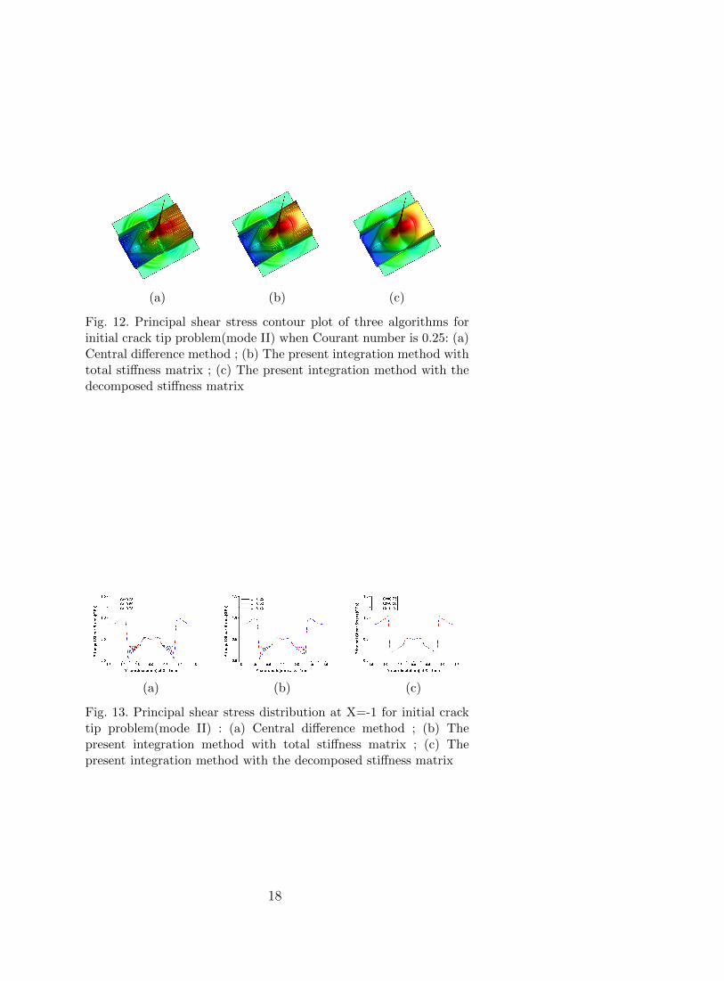
A plane strain problem with crack as shown in Fig. 11 is sub-jected to a mode-II type incident wave. Figure 12 shows a con-tour plot of principal shear stress after the wave is reflected fromthe crack tip. Notice that the stress distribution computed bythe central difference method and the integration method withtotal stiffness matrix yield a saw-tooth pattern which indicatesconsiderable spurious oscillations as shown in the left of Fig.12. On the other hand, the stress contour plot by the presentmethod with the decomposed equation does not exhibit suchsaw-tooth oscillations as shown in Fig. 13.

(a) (b)

Fig. 11. Plane strain rectangular model problem(mode II) with initialcrack tip subjected to a Heaviside initial velocity input: (a) Geometryand boundary conditions; (b) Analytical solution

17

(a) (b) (c)

Fig. 12. Principal shear stress contour plot of three algorithms forinitial crack tip problem(mode II) when Courant number is 0.25: (a)Central difference method ; (b) The present integration method withtotal stiffness matrix ; (c) The present integration method with thedecomposed stiffness matrix

(a) (b) (c)

Fig. 13. Principal shear stress distribution at X=-1 for initial cracktip problem(mode II) : (a) Central difference method ; (b) Thepresent integration method with total stiffness matrix ; (c) Thepresent integration method with the decomposed stiffness matrix

18