ascat l2 winds data record validation reportprojects.knmi.nl/scatterometer/publications/pdf/... ·...

Ocean and Sea Ice SAF

Technical Note SAF/OSI/CDOP2/KNMI/TEC/RP/239

ASCAT L2 winds Data Record validation report

25 km and 12.5 km coastal wind products (OSI-150-a and OSI-150-b) DOI: 10.15770/EUM_SAF_OSI_0006, 10.15770/EUM_SAF_OSI_0007

Anton Verhoef, Jur Vogelzang and Ad Stoffelen KNMI

Version 1.2

July 2016

SAF/OSI/CDOP2/KNMI/TEC/RP/239 ASCAT L2 winds Data Record validation report

of 20

DOCUMENTATION CHANGE RECORD

Issue / Revision Date Change Description

Version 1.0 Nov 2015 Draft version

Version 1.1 Jan 2016 Minor Changes according to comments from DRR

Version 1.2 Jul 2016 Minor Final version for release.

KNMI, De Bilt, the Netherlands Reference: SAF/OSI/CDOP2/KNMI/TEC/RP/239


of 20

Contents 1 Introduction .............................................................................................................................. 4

2 Backscatter data stability ........................................................................................................ 5

3 Quality Control characteristics ............................................................................................... 6

4 Comparison of winds with NWP model and buoys .............................................................. 7

4.1 NWP model wind comparisons .................................................................................................. 7 4.2 Buoy wind comparisons ............................................................................................................. 9

5 Triple collocation results .......................................................................................................14

6 Conclusions ............................................................................................................................16

7 References ..............................................................................................................................17

8 Abbreviations and acronyms ................................................................................................19

9 Appendix A: List of used buoys ...........................................................................................20


of 20

1 Introduction The EUMETSAT Ocean and Sea Ice Satellite Application Facility (OSI SAF) produces a range of air-sea interface products, namely: wind, sea ice characteristics, Sea Surface Temperatures (SST) and radiative fluxes, Surface Solar Irradiance (SSI) and Downward Long wave Irradiance (DLI). The Product Requirements Document [1] provides an overview of the committed products and their characteristics in the current OSI SAF project phase, the Service Specification Document [2] provides specifications and detailed information on the services committed towards the users by the OSI SAF in a given stage of the project. This report contains validation information about the Metop-A/ASCAT wind Climate Data Record (CDR), produced in the OSI SAF. The reprocessed level 1b data record, spanning the period of 1 January 2007 to 31 March 2014 was obtained from the EUMETSAT Data Centre. The data have been processed using the ASCAT Wind Data Processor (AWDP) software version 2.4, as available in the Numerical Weather Prediction (NWP) SAF [3]. More information about the processing and the products can be obtained from the Product User Manual [4]. The quality and stability of the ASCAT wind CDR has been assessed by looking both at backscatter and wind data. Section 2 describes the checks on the backscatter stability over time. Section 3 assesses the Quality Control applied in the products. In section 4, the winds are compared with NWP model data and with wind data from in situ buoys. Section 5 describes triple collocation experiments to assess the quality of winds from scatterometer, NWP model and buoys separately. Section 6 summarises the main conclusions.

Acknowledgement We are grateful to Jean Bidlot of ECMWF for helping us with the buoy data retrieval and quality control.


of 20

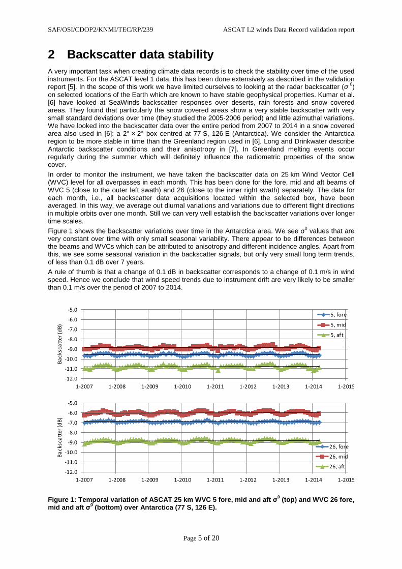
2 Backscatter data stability A very important task when creating climate data records is to check the stability over time of the used instruments. For the ASCAT level 1 data, this has been done extensively as described in the validation report [5]. In the scope of this work we have limited ourselves to looking at the radar backscatter (σ 0) on selected locations of the Earth which are known to have stable geophysical properties. Kumar et al. [6] have looked at SeaWinds backscatter responses over deserts, rain forests and snow covered areas. They found that particularly the snow covered areas show a very stable backscatter with very small standard deviations over time (they studied the 2005-2006 period) and little azimuthal variations. We have looked into the backscatter data over the entire period from 2007 to 2014 in a snow covered area also used in [6]: a 2° × 2° box centred at 77 S, 126 E (Antarctica). We consider the Antarctica region to be more stable in time than the Greenland region used in [6]. Long and Drinkwater describe Antarctic backscatter conditions and their anisotropy in [7]. In Greenland melting events occur regularly during the summer which will definitely influence the radiometric properties of the snow cover. In order to monitor the instrument, we have taken the backscatter data on 25 km Wind Vector Cell (WVC) level for all overpasses in each month. This has been done for the fore, mid and aft beams of WVC 5 (close to the outer left swath) and 26 (close to the inner right swath) separately. The data for each month, i.e., all backscatter data acquisitions located within the selected box, have been averaged. In this way, we average out diurnal variations and variations due to different flight directions in multiple orbits over one month. Still we can very well establish the backscatter variations over longer time scales. Figure 1 shows the backscatter variations over time in the Antarctica area. We see σ0 values that are very constant over time with only small seasonal variability. There appear to be differences between the beams and WVCs which can be attributed to anisotropy and different incidence angles. Apart from this, we see some seasonal variation in the backscatter signals, but only very small long term trends, of less than 0.1 dB over 7 years. A rule of thumb is that a change of 0.1 dB in backscatter corresponds to a change of 0.1 m/s in wind speed. Hence we conclude that wind speed trends due to instrument drift are very likely to be smaller than 0.1 m/s over the period of 2007 to 2014.

Figure 1: Temporal variation of ASCAT 25 km WVC 5 fore, mid and aft σ0 (top) and WVC 26 fore, mid and aft σ0 (bottom) over Antarctica (77 S, 126 E).

-12.0

-11.0

-10.0

-9.0

-8.0

-7.0

-6.0

-5.0

1-2007 1-2008 1-2009 1-2010 1-2011 1-2012 1-2013 1-2014 1-2015

Back

scat

ter (

dB)

5, fore

5, mid

5, aft

-12.0

-11.0

-10.0

-9.0

-8.0

-7.0

-6.0

-5.0

1-2007 1-2008 1-2009 1-2010 1-2011 1-2012 1-2013 1-2014 1-2015

Back

scat

ter (

dB)

26, fore

26, mid

26, aft


of 20

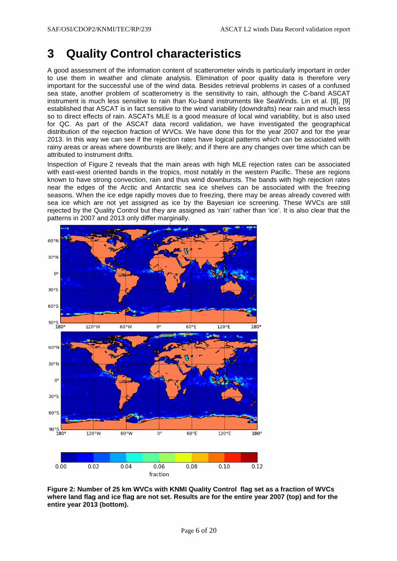
3 Quality Control characteristics A good assessment of the information content of scatterometer winds is particularly important in order to use them in weather and climate analysis. Elimination of poor quality data is therefore very important for the successful use of the wind data. Besides retrieval problems in cases of a confused sea state, another problem of scatterometry is the sensitivity to rain, although the C-band ASCAT instrument is much less sensitive to rain than Ku-band instruments like SeaWinds. Lin et al. [8], [9] established that ASCAT is in fact sensitive to the wind variability (downdrafts) near rain and much less so to direct effects of rain. ASCATs MLE is a good measure of local wind variability, but is also used for QC. As part of the ASCAT data record validation, we have investigated the geographical distribution of the rejection fraction of WVCs. We have done this for the year 2007 and for the year 2013. In this way we can see if the rejection rates have logical patterns which can be associated with rainy areas or areas where downbursts are likely; and if there are any changes over time which can be attributed to instrument drifts. Inspection of Figure 2 reveals that the main areas with high MLE rejection rates can be associated with east-west oriented bands in the tropics, most notably in the western Pacific. These are regions known to have strong convection, rain and thus wind downbursts. The bands with high rejection rates near the edges of the Arctic and Antarctic sea ice shelves can be associated with the freezing seasons. When the ice edge rapidly moves due to freezing, there may be areas already covered with sea ice which are not yet assigned as ice by the Bayesian ice screening. These WVCs are still rejected by the Quality Control but they are assigned as ‘rain’ rather than ‘ice’. It is also clear that the patterns in 2007 and 2013 only differ marginally.

Figure 2: Number of 25 km WVCs with KNMI Quality Control flag set as a fraction of WVCs where land flag and ice flag are not set. Results are for the entire year 2007 (top) and for the entire year 2013 (bottom).


of 20

4 Comparison of winds with NWP model and buoys 4.1 NWP model wind comparisons

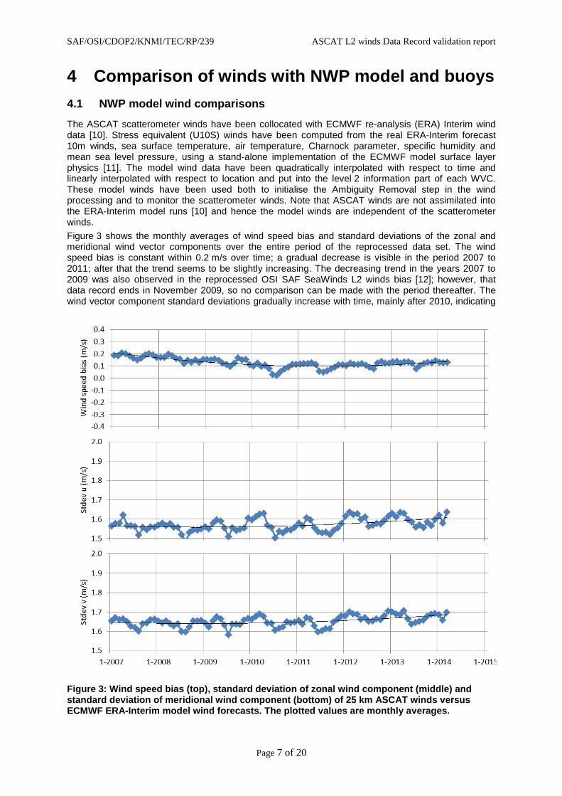
The ASCAT scatterometer winds have been collocated with ECMWF re-analysis (ERA) Interim wind data [10]. Stress equivalent (U10S) winds have been computed from the real ERA-Interim forecast 10m winds, sea surface temperature, air temperature, Charnock parameter, specific humidity and mean sea level pressure, using a stand-alone implementation of the ECMWF model surface layer physics [11]. The model wind data have been quadratically interpolated with respect to time and linearly interpolated with respect to location and put into the level 2 information part of each WVC. These model winds have been used both to initialise the Ambiguity Removal step in the wind processing and to monitor the scatterometer winds. Note that ASCAT winds are not assimilated into the ERA-Interim model runs [10] and hence the model winds are independent of the scatterometer winds. Figure 3 shows the monthly averages of wind speed bias and standard deviations of the zonal and meridional wind vector components over the entire period of the reprocessed data set. The wind speed bias is constant within 0.2 m/s over time; a gradual decrease is visible in the period 2007 to 2011; after that the trend seems to be slightly increasing. The decreasing trend in the years 2007 to 2009 was also observed in the reprocessed OSI SAF SeaWinds L2 winds bias [12]; however, that data record ends in November 2009, so no comparison can be made with the period thereafter. The wind vector component standard deviations gradually increase with time, mainly after 2010, indicating

Figure 3: Wind speed bias (top), standard deviation of zonal wind component (middle) and standard deviation of meridional wind component (bottom) of 25 km ASCAT winds versus ECMWF ERA-Interim model wind forecasts. The plotted values are monthly averages.


of 20

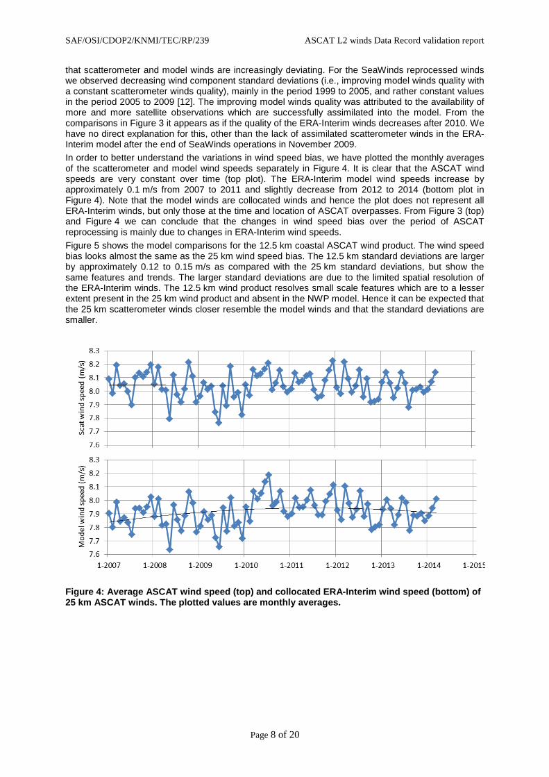
that scatterometer and model winds are increasingly deviating. For the SeaWinds reprocessed winds we observed decreasing wind component standard deviations (i.e., improving model winds quality with a constant scatterometer winds quality), mainly in the period 1999 to 2005, and rather constant values in the period 2005 to 2009 [12]. The improving model winds quality was attributed to the availability of more and more satellite observations which are successfully assimilated into the model. From the comparisons in Figure 3 it appears as if the quality of the ERA-Interim winds decreases after 2010. We have no direct explanation for this, other than the lack of assimilated scatterometer winds in the ERA-Interim model after the end of SeaWinds operations in November 2009. In order to better understand the variations in wind speed bias, we have plotted the monthly averages of the scatterometer and model wind speeds separately in Figure 4. It is clear that the ASCAT wind speeds are very constant over time (top plot). The ERA-Interim model wind speeds increase by approximately 0.1 m/s from 2007 to 2011 and slightly decrease from 2012 to 2014 (bottom plot in Figure 4). Note that the model winds are collocated winds and hence the plot does not represent all ERA-Interim winds, but only those at the time and location of ASCAT overpasses. From Figure 3 (top) and Figure 4 we can conclude that the changes in wind speed bias over the period of ASCAT reprocessing is mainly due to changes in ERA-Interim wind speeds. Figure 5 shows the model comparisons for the 12.5 km coastal ASCAT wind product. The wind speed bias looks almost the same as the 25 km wind speed bias. The 12.5 km standard deviations are larger by approximately 0.12 to 0.15 m/s as compared with the 25 km standard deviations, but show the same features and trends. The larger standard deviations are due to the limited spatial resolution of the ERA-Interim winds. The 12.5 km wind product resolves small scale features which are to a lesser extent present in the 25 km wind product and absent in the NWP model. Hence it can be expected that the 25 km scatterometer winds closer resemble the model winds and that the standard deviations are smaller.

Figure 4: Average ASCAT wind speed (top) and collocated ERA-Interim wind speed (bottom) of 25 km ASCAT winds. The plotted values are monthly averages.


of 20

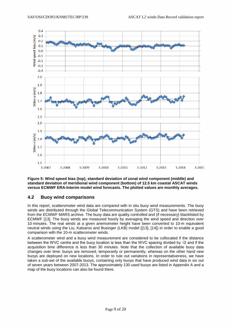
Figure 5: Wind speed bias (top), standard deviation of zonal wind component (middle) and standard deviation of meridional wind component (bottom) of 12.5 km coastal ASCAT winds versus ECMWF ERA-Interim model wind forecasts. The plotted values are monthly averages.

4.2 Buoy wind comparisons

In this report, scatterometer wind data are compared with in situ buoy wind measurements. The buoy winds are distributed through the Global Telecommunication System (GTS) and have been retrieved from the ECMWF MARS archive. The buoy data are quality controlled and (if necessary) blacklisted by ECMWF [13]. The buoy winds are measured hourly by averaging the wind speed and direction over 10 minutes. The real winds at a given anemometer height have been converted to 10-m equivalent neutral winds using the Liu, Katsaros and Businger (LKB) model ([13], [14]) in order to enable a good comparison with the 10-m scatterometer winds. A scatterometer wind and a buoy wind measurement are considered to be collocated if the distance between the WVC centre and the buoy location is less than the WVC spacing divided by √2 and if the acquisition time difference is less than 30 minutes. Note that the collection of available buoy data changes over time: buoys are removed, temporarily or permanently, whereas on the other hand new buoys are deployed on new locations. In order to rule out variations in representativeness, we have taken a sub-set of the available buoys, containing only buoys that have produced wind data in six out of seven years between 2007-2013. The approximately 130 used buoys are listed in Appendix A and a map of the buoy locations can also be found there.


of 20

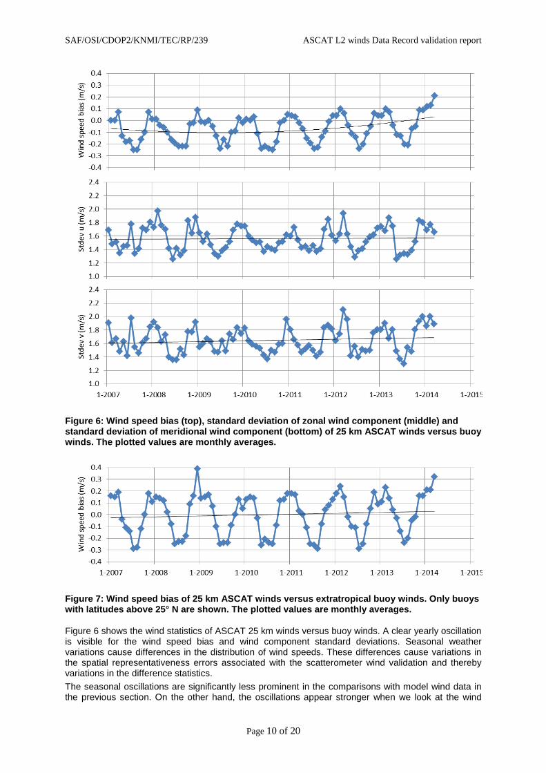
Figure 6: Wind speed bias (top), standard deviation of zonal wind component (middle) and standard deviation of meridional wind component (bottom) of 25 km ASCAT winds versus buoy winds. The plotted values are monthly averages.

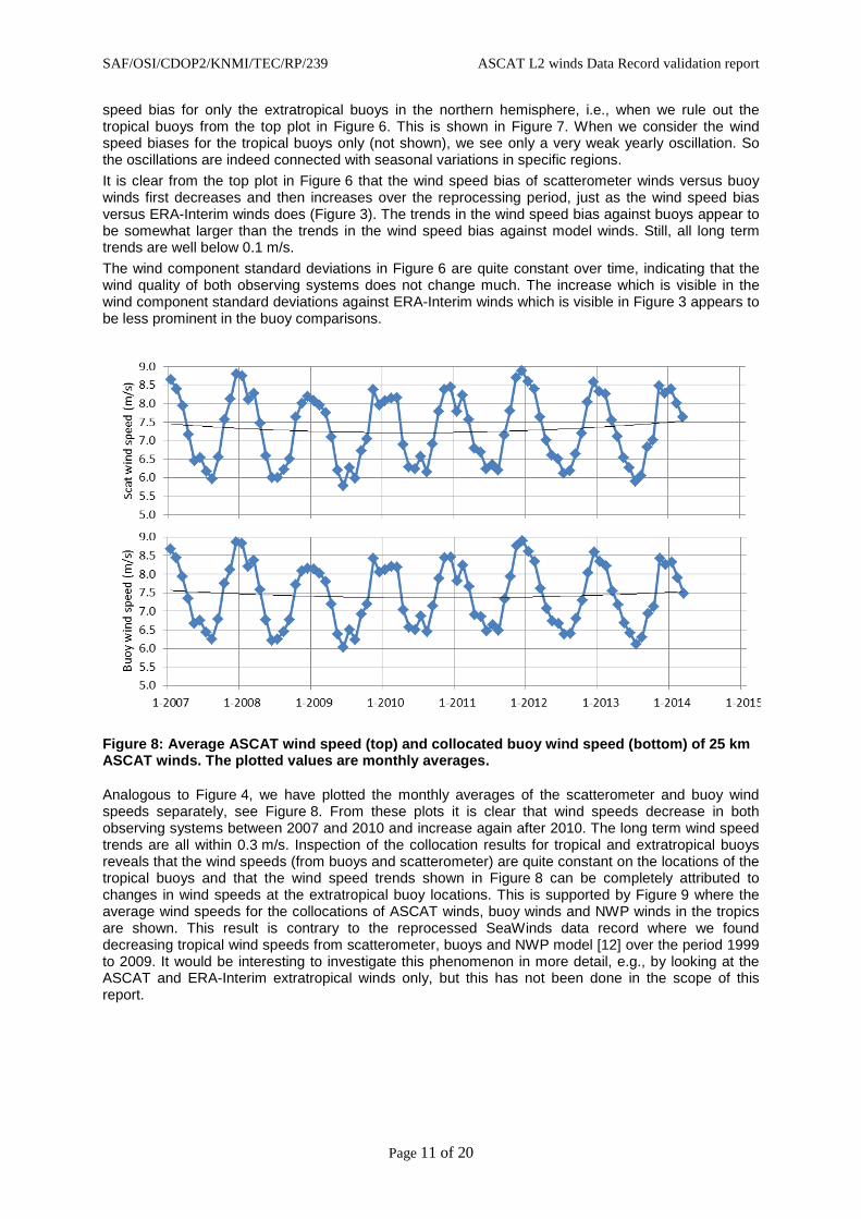
Figure 7: Wind speed bias of 25 km ASCAT winds versus extratropical buoy winds. Only buoys with latitudes above 25° N are shown. The plotted values are monthly averages.

Figure 6 shows the wind statistics of ASCAT 25 km winds versus buoy winds. A clear yearly oscillation is visible for the wind speed bias and wind component standard deviations. Seasonal weather variations cause differences in the distribution of wind speeds. These differences cause variations in the spatial representativeness errors associated with the scatterometer wind validation and thereby variations in the difference statistics. The seasonal oscillations are significantly less prominent in the comparisons with model wind data in the previous section. On the other hand, the oscillations appear stronger when we look at the wind


of 20

speed bias for only the extratropical buoys in the northern hemisphere, i.e., when we rule out the tropical buoys from the top plot in Figure 6. This is shown in Figure 7. When we consider the wind speed biases for the tropical buoys only (not shown), we see only a very weak yearly oscillation. So the oscillations are indeed connected with seasonal variations in specific regions. It is clear from the top plot in Figure 6 that the wind speed bias of scatterometer winds versus buoy winds first decreases and then increases over the reprocessing period, just as the wind speed bias versus ERA-Interim winds does (Figure 3). The trends in the wind speed bias against buoys appear to be somewhat larger than the trends in the wind speed bias against model winds. Still, all long term trends are well below 0.1 m/s. The wind component standard deviations in Figure 6 are quite constant over time, indicating that the wind quality of both observing systems does not change much. The increase which is visible in the wind component standard deviations against ERA-Interim winds which is visible in Figure 3 appears to be less prominent in the buoy comparisons.

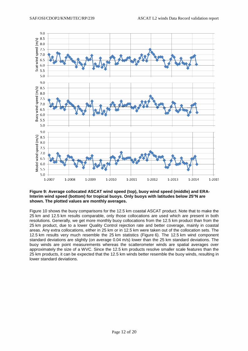
Figure 8: Average ASCAT wind speed (top) and collocated buoy wind speed (bottom) of 25 km ASCAT winds. The plotted values are monthly averages.

Analogous to Figure 4, we have plotted the monthly averages of the scatterometer and buoy wind speeds separately, see Figure 8. From these plots it is clear that wind speeds decrease in both observing systems between 2007 and 2010 and increase again after 2010. The long term wind speed trends are all within 0.3 m/s. Inspection of the collocation results for tropical and extratropical buoys reveals that the wind speeds (from buoys and scatterometer) are quite constant on the locations of the tropical buoys and that the wind speed trends shown in Figure 8 can be completely attributed to changes in wind speeds at the extratropical buoy locations. This is supported by Figure 9 where the average wind speeds for the collocations of ASCAT winds, buoy winds and NWP winds in the tropics are shown. This result is contrary to the reprocessed SeaWinds data record where we found decreasing tropical wind speeds from scatterometer, buoys and NWP model [12] over the period 1999 to 2009. It would be interesting to investigate this phenomenon in more detail, e.g., by looking at the ASCAT and ERA-Interim extratropical winds only, but this has not been done in the scope of this report.


of 20

Figure 9: Average collocated ASCAT wind speed (top), buoy wind speed (middle) and ERA-Interim wind speed (bottom) for tropical buoys. Only buoys with latitudes below 25°N are shown. The plotted values are monthly averages.

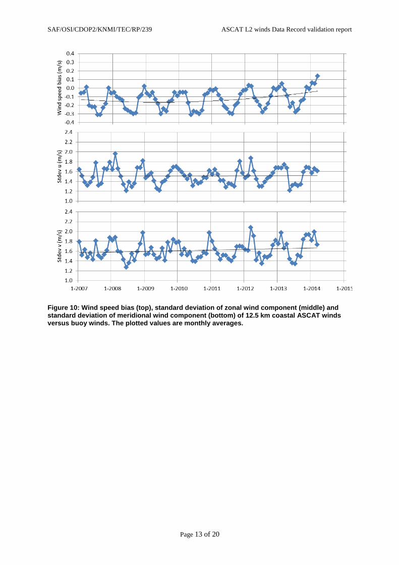
Figure 10 shows the buoy comparisons for the 12.5 km coastal ASCAT product. Note that to make the 25 km and 12.5 km results comparable, only those collocations are used which are present in both resolutions. Generally, we get more monthly buoy collocations from the 12.5 km product than from the 25 km product, due to a lower Quality Control rejection rate and better coverage, mainly in coastal areas. Any extra collocations, either in 25 km or in 12.5 km were taken out of the collocation sets. The 12.5 km results very much resemble the 25 km statistics (Figure 6). The 12.5 km wind component standard deviations are slightly (on average 0.04 m/s) lower than the 25 km standard deviations. The buoy winds are point measurements whereas the scatterometer winds are spatial averages over approximately the size of a WVC. Since the 12.5 km products resolve smaller scale features than the 25 km products, it can be expected that the 12.5 km winds better resemble the buoy winds, resulting in lower standard deviations.


of 20

Figure 10: Wind speed bias (top), standard deviation of zonal wind component (middle) and standard deviation of meridional wind component (bottom) of 12.5 km coastal ASCAT winds versus buoy winds. The plotted values are monthly averages.


of 20

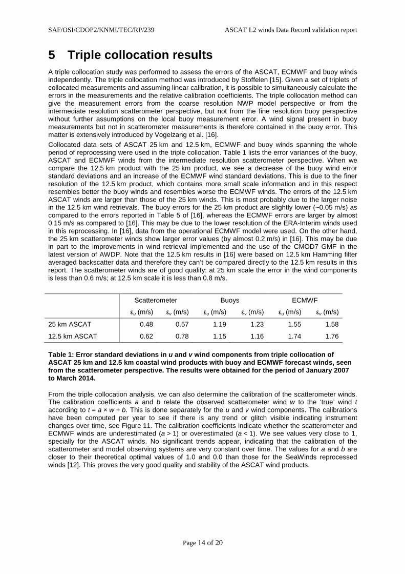
5 Triple collocation results A triple collocation study was performed to assess the errors of the ASCAT, ECMWF and buoy winds independently. The triple collocation method was introduced by Stoffelen [15]. Given a set of triplets of collocated measurements and assuming linear calibration, it is possible to simultaneously calculate the errors in the measurements and the relative calibration coefficients. The triple collocation method can give the measurement errors from the coarse resolution NWP model perspective or from the intermediate resolution scatterometer perspective, but not from the fine resolution buoy perspective without further assumptions on the local buoy measurement error. A wind signal present in buoy measurements but not in scatterometer measurements is therefore contained in the buoy error. This matter is extensively introduced by Vogelzang et al. [16]. Collocated data sets of ASCAT 25 km and 12.5 km, ECMWF and buoy winds spanning the whole period of reprocessing were used in the triple collocation. Table 1 lists the error variances of the buoy, ASCAT and ECMWF winds from the intermediate resolution scatterometer perspective. When we compare the 12.5 km product with the 25 km product, we see a decrease of the buoy wind error standard deviations and an increase of the ECMWF wind standard deviations. This is due to the finer resolution of the 12.5 km product, which contains more small scale information and in this respect resembles better the buoy winds and resembles worse the ECMWF winds. The errors of the 12.5 km ASCAT winds are larger than those of the 25 km winds. This is most probably due to the larger noise in the 12.5 km wind retrievals. The buoy errors for the 25 km product are slightly lower (~0.05 m/s) as compared to the errors reported in Table 5 of [16], whereas the ECMWF errors are larger by almost 0.15 m/s as compared to [16]. This may be due to the lower resolution of the ERA-Interim winds used in this reprocessing. In [16], data from the operational ECMWF model were used. On the other hand, the 25 km scatterometer winds show larger error values (by almost 0.2 m/s) in [16]. This may be due in part to the improvements in wind retrieval implemented and the use of the CMOD7 GMF in the latest version of AWDP. Note that the 12.5 km results in [16] were based on 12.5 km Hamming filter averaged backscatter data and therefore they can’t be compared directly to the 12.5 km results in this report. The scatterometer winds are of good quality: at 25 km scale the error in the wind components is less than 0.6 m/s; at 12.5 km scale it is less than 0.8 m/s.

Scatterometer Buoys ECMWF

εu (m/s) εv (m/s) εu (m/s) εv (m/s) εu (m/s) εv (m/s)

25 km ASCAT 0.48 0.57 1.19 1.23 1.55 1.58

12.5 km ASCAT 0.62 0.78 1.15 1.16 1.74 1.76

Table 1: Error standard deviations in u and v wind components from triple collocation of ASCAT 25 km and 12.5 km coastal wind products with buoy and ECMWF forecast winds, seen from the scatterometer perspective. The results were obtained for the period of January 2007 to March 2014.

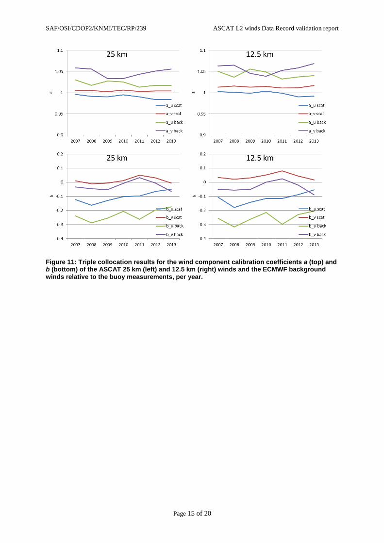
From the triple collocation analysis, we can also determine the calibration of the scatterometer winds. The calibration coefficients a and b relate the observed scatterometer wind w to the ‘true’ wind t according to t = a × w + b. This is done separately for the u and v wind components. The calibrations have been computed per year to see if there is any trend or glitch visible indicating instrument changes over time, see Figure 11. The calibration coefficients indicate whether the scatterometer and ECMWF winds are underestimated (a > 1) or overestimated (a < 1). We see values very close to 1, specially for the ASCAT winds. No significant trends appear, indicating that the calibration of the scatterometer and model observing systems are very constant over time. The values for a and b are closer to their theoretical optimal values of 1.0 and 0.0 than those for the SeaWinds reprocessed winds [12]. This proves the very good quality and stability of the ASCAT wind products.


of 20

Figure 11: Triple collocation results for the wind component calibration coefficients a (top) and b (bottom) of the ASCAT 25 km (left) and 12.5 km (right) winds and the ECMWF background winds relative to the buoy measurements, per year.


of 20

6 Conclusions The quality and stability of the ASCAT CDR has been assessed by looking both at backscatter and wind data. The backscatter values appear to be very constant in time over a selected area on Antarctica. For different swath locations (WVC numbers), we obtain time series with long term trends of less than 0.1 dB. From these very stable results, we conclude that the observed ASCAT backscatter drifts appear negligible. The scatterometer wind biases against ERA-Interim and buoy winds show some long term trends, a gradual decrease followed by some increase but those trends appear to be within 0.1 m/s over a period of more than 7 years. Inspection of the data in different regions on the Earth reveals that there is a relatively large variability in bias results depending on season and climatological region. Nevertheless, the analysed ASCAT backscatter and wind changes suggest variations in instrumental bias of well less than 0.1 dB (equivalent to 0.1 m/s) in seven years. As such, the produced ASCAT wind data record meets the requirements set by the World Climate Research Programme (WCRP) [17]: accuracy better than 0.5 m/s, stability better than 0.1 m/s per decade. From the figures in section 4, we conclude that the OSI SAF product requirements ([1], better than 2 m/s in wind component standard deviation with a bias of less than 0.5 m/s in wind speed on a monthly basis) are also well met. The triple collocation results show that the scatterometer winds are of good quality, well calibrated and very stable over time. In the scope of this validation report, no attempt was made to connect the bias and standard deviation changes over time to decadal and inter-annual climate oscillations, such as the Madden–Julian oscillation (MJO), the Pacific Decadal Oscillation (PDO), the El Niño–Southern Oscillation (ENSO), and the North Atlantic Oscillation (NAO). We hope that climate scientists will use the CDR to better understand and explain these phenomena.


of 20

7 References [1] OSI SAF,

Product Requirements Document SAF/OSI/CDOP2/M-F/MGT/PL/2-001, 2015

[2] OSI SAF, Service Specification Document SAF/OSI/CDOP2/M-F/MGT/PL/2-003, 2015

[3] Vogelzang, J., A. Verhoef, J. Verspeek, J. de Kloe and A. Stoffelen, AWDP User Manual and Reference Guide NWPSAF-KN-UD-005, 2015

[4] OSI SAF, ASCAT L2 winds Data Record Product User Manual SAF/OSI/CDOP2/KNMI/TEC/MA/238, 2015

[5] EUMETSAT, Metop-A ASCAT L1 Data Record (CF-003) Release 2: Validation Report EUM/OPS-EPS/REP/14/753112, 2014

[6] Kumar, R., S.A. Bhowmick, K. N. Babu, R. Nigam, and A. Sarkar, Relative Calibration Using Natural Terrestrial Targets: A Preparation Towards Oceansat-2 Scatterometer IEEE Transactions on Geoscience and Remote Sensing, 49, 6, 2268-2273, 2011, doi:10.1109/TGRS.2010.2094196

[7] Long, D. and M. Drinkwater, Azimuth variation in microwave scatterometer and radiometer data over Antarctica IEEE Transactions on Geoscience and Remote Sensing, 38, 4, 1857-1870, 2000, doi:10.1109/36.851769

[8] Lin, W., M. Portabella, A. Stoffelen, A. Verhoef en A. Turiel, ASCAT Wind Quality Control Near Rain IEEE Transactions on Geoscience and Remote Sensing, 53, 8, 2015, 4165-4177, doi:10.1109/TGRS.2015.2392372

[9] Lin, W., M. Portabella, A. Stoffelen, J. Vogelzang en A. Verhoef, ASCAT wind quality under high subcell wind variability conditions J. Geophys. Res. Oceans, 120, 8, 2015, 5804-5819, doi:10.1002/2015JC010861

[10] Dee, D. et al., The ERA-Interim reanalysis: configuration and performance of the data assimilation system Quarterly Journal of the Royal Meteorological Society, 137: 553–597, 2011, doi:10.1002/qj.828

[11] Hersbach, H., Assimilation of scatterometer data as equivalent-neutral wind ECMWF Technical Memorandum 629, 2010

[12] Verhoef, A., J. Vogelzang and A. Stoffelen, Reprocessed SeaWinds L2 winds validation report SAF/OSI/CDOP2/KNMI/TEC/RP/221, 2015

[13] Bidlot J., D. Holmes, P. Wittmann, R. Lalbeharry, and H. Chen Intercomparison of the performance of operational ocean wave forecasting systems with buoy data Wea. Forecasting, vol. 17, 287-310, 2002

[14] Liu, W.T., K.B. Katsaros, and J.A. Businger Bulk parameterization of air-sea exchanges of heat and water vapor including the molecular constraints in the interface J. Atmos. Sci., vol. 36, 1979

[15] Stoffelen, A. Toward the true near-surface wind speed: error modeling and calibration using triple collocation J. Geophys. Res. 103, C4, 7755-7766, 1998, doi:10.1029/97JC03180

[16] Vogelzang, J., A. Stoffelen, A. Verhoef and J. Figa-Saldana On the quality of high-resolution scatterometer winds J. Geophys. Res., 116, C10033, 2011, doi:10.1029/2010JC006640


of 20

[17] Global Climate Observing System, Systematic Observation Requirements for Satellite-based Products for Climate Supplemental details to the satellite-based component of the Implementation Plan for the Global Observing System for Climate in Support of the UNFCCC - 2011 Update, December 2011, GCOS Report 154, http://www.wmo.int/pages/prog/gcos/Publications/gcos-154.pdf

http://www.wmo.int/pages/prog/gcos/Publications/gcos-154.pdf


of 20

8 Abbreviations and acronyms 2DVAR Two-dimensional Variational Ambiguity Removal ASCAT Advanced Scatterometer AWDP ASCAT Wind Data Processor CDR Climate Data Record ECMWF European Centre for Medium-Range Weather Forecasts ERA ECMWF re-analysis EUMETSAT European Organisation for the Exploitation of Meteorological Satellites GTS Global Telecommunication System KNMI Royal Netherlands Meteorological Institute LKB Liu, Katsaros and Businger NOAA National Oceanic and Atmospheric Administration NWP Numerical Weather Prediction OSI Ocean and Sea Ice QC Quality Control QuikSCAT US Quick Scatterometer mission carrying the SeaWinds scatterometer SAF Satellite Application Facility u West-to-east (zonal) wind component v South-to-north (meridional) wind component WCRP World Climate Research Programme WVC Wind Vector Cell


of 20

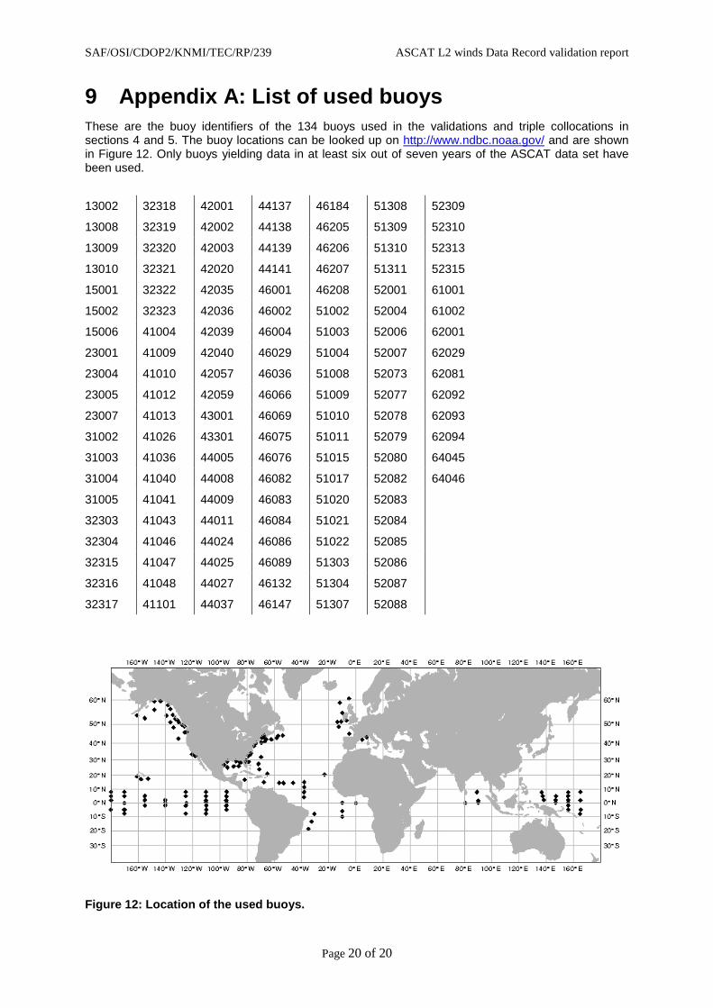
9 Appendix A: List of used buoys These are the buoy identifiers of the 134 buoys used in the validations and triple collocations in sections 4 and 5. The buoy locations can be looked up on http://www.ndbc.noaa.gov/ and are shown in Figure 12. Only buoys yielding data in at least six out of seven years of the ASCAT data set have been used.

13002 32318 42001 44137 46184 51308 52309

13008 32319 42002 44138 46205 51309 52310

13009 32320 42003 44139 46206 51310 52313

13010 32321 42020 44141 46207 51311 52315

15001 32322 42035 46001 46208 52001 61001

15002 32323 42036 46002 51002 52004 61002

15006 41004 42039 46004 51003 52006 62001

23001 41009 42040 46029 51004 52007 62029

23004 41010 42057 46036 51008 52073 62081

23005 41012 42059 46066 51009 52077 62092

23007 41013 43001 46069 51010 52078 62093

31002 41026 43301 46075 51011 52079 62094

31003 41036 44005 46076 51015 52080 64045

31004 41040 44008 46082 51017 52082 64046

31005 41041 44009 46083 51020 52083

32303 41043 44011 46084 51021 52084

32304 41046 44024 46086 51022 52085

32315 41047 44025 46089 51303 52086

32316 41048 44027 46132 51304 52087

32317 41101 44037 46147 51307 52088

Figure 12: Location of the used buoys.

http://www.ndbc.noaa.gov/

ascat l2 winds data record validation reportprojects.knmi.nl/scatterometer/publications/pdf/... ·...

Documents