asap3: a batch means procedure for steady-state simulation
TRANSCRIPT

ASAP3: A Batch Means Procedure forSteady-State Simulation Analysis
NATALIE M. STEIGERUniversity of MaineEMILY K. LADAStatistical and Applied Mathematical Sciences InstituteJAMES R. WILSON and JEFFREY A. JOINESNorth Carolina State UniversityandCHRISTOS ALEXOPOULOS and DAVID GOLDSMANGeorgia Institute of Technology
We introduce ASAP3, a refinement of the batch means algorithms ASAP and ASAP2, that deliverspoint and confidence-interval estimators for the expected response of a steady-state simulation.ASAP3 is a sequential procedure designed to produce a confidence-interval estimator that satis-fies user-specified requirements on absolute or relative precision as well as coverage probability.ASAP3 operates as follows: the batch size is progressively increased until the batch means passthe Shapiro-Wilk test for multivariate normality; and then ASAP3 fits a first-order autoregressive(AR(1)) time series model to the batch means. If necessary, the batch size is further increased untilthe autoregressive parameter in the AR(1) model does not significantly exceed 0.8. Next, ASAP3computes the terms of an inverse Cornish-Fisher expansion for the classical batch means t-ratiobased on the AR(1) parameter estimates; and finally ASAP3 delivers a correlation-adjusted con-fidence interval based on this expansion. Regarding not only conformance to the precision andcoverage-probability requirements but also the mean and variance of the half-length of the de-livered confidence interval, ASAP3 compared favorably to other batch means procedures (namely,ABATCH, ASAP, ASAP2, and LBATCH) in an extensive experimental performance evaluation.
This work was partially supported by the National Science Foundation under grant number DMI-9900164.This article was submitted and reviewed under the editorship of David Nicol.Authors’ addresses: N. M. Steiger, Maine Business School, University of Maine, Orono, ME 04469-5723; email: [email protected]; E. K. Lada, Statistical and Applied Mathematical Sciences Insti-tute, Research Triangle Park, NC 27709-4006; email: [email protected]; J. R. Wilson, Departmentof Industrial Engineering, Box 7906, North Carolina State University, Raleigh, NC 27695-7906;email: [email protected]; J. A. Joines, Department of Textile Engineering, Chemistry, and Science,Box 8301, North Carolina State University, Raleigh, NC 27695-8301; email: [email protected];C. Alexopoulos and D. Goldsman, School of Industrial and Systems Engineering, Georgia Instituteof Technology, Atlanta, GA 30332; email: {christos,sman}@isye.gatech.edu.Permission to make digital or hard copies of part or all of this work for personal or classroom use isgranted without fee provided that copies are not made or distributed for profit or direct commercialadvantage and that copies show this notice on the first page or initial screen of a display alongwith the full citation. Copyrights for components of this work owned by others than ACM must behonored. Abstracting with credit is permitted. To copy otherwise, to republish, to post on servers,to redistribute to lists, or to use any component of this work in other works requires prior specificpermission and/or a fee. Permissions may be requested from Publications Dept., ACM, Inc., 1515Broadway, New York, NY 10036 USA, fax: +1 (212) 869-0481, or [email protected]© 2005 ACM 1049-3301/05/0100-0039 $5.00
ACM Transactions on Modeling and Computer Simulation, Vol. 15, No. 1, January 2005, Pages 39–73.
40 • N. M. Steiger et al.
Categories and Subject Descriptors: G.3 [Mathematics of Computing]: Probability and Statis-tics—Time series analysis; I.6.6 [Simulation and Modeling]: Simulation output analysis
General Terms: Experimentation, Measurement, Performance, Theory
Additional Key Words and Phrases: Batch means, confidence interval estimation, inverse Cornish-Fisher expansion, sequential analysis, simulation start-up problem, steady-state simulation
1. INTRODUCTION
In discrete-event simulation, we are often interested in estimating the steady-state mean µX of a stochastic output process {X j : j = 1, 2, . . .} generated bya single, prolonged simulation run. Assuming the target process is stationary,and given a time series of length n that is part of a single realization of thisprocess, we see that a natural point estimator of µX is the sample mean, givenby X (n) = n−1 ∑n
j=1 X j . We also require some indication of the precision ofthis point estimator; and typically we construct a confidence interval (CI) forµX with a user-specified probability 1 − α of covering the point µX , where0 < α < 1. The CI for µX should satisfy two criteria: (i) it is approximatelyvalid—that is, its coverage probability is sufficiently close to the nominal level1 − α; and (ii) it has sufficient precision—that is, it is narrow enough—to bemeaningful in the context of the application at hand.
In the simulation analysis method of nonoverlapping batch means (NOBM),the sequence of simulation-generated outputs {X j : j = 1, . . . , n} is divided intok adjacent nonoverlapping batches, each of size m. For simplicity, we assumethat n is a multiple of m so that n = km. The sample mean for the j th batch is
Y j (m) = 1m
mj∑i=m( j−1)+1
X i for j = 1, . . . , k; (1)
and the grand mean of the individual batch means,
Y = Y (m, k) = 1k
k∑j=1
Y j (m), (2)
is used as a point estimator for µX (note that Y (m, k) = X (n)). We construct a CIestimator for µX that is centered on a point estimator like (2), where, in practice,we may exclude some initial batches to eliminate the effects of start-up bias.
If the batch size m is sufficiently large so that the batch means {Y j (m) :j = 1, . . . , k} are approximately independent and identically distributed (i.i.d.)normal random variables with mean µX , then we can apply classical results con-cerning Student’s t-distribution (see, for example, Alexopoulos and Goldsman[2004]) to compute a CI for µX from the batch means. For this purpose, wecompute the sample variance of the k batch means for batches of size m,
S2m,k = 1
k − 1
k∑j=1
[Y j(m) − Y(m, k)]2.
If the original simulation-generated process {X j : j = 1, . . . , n} is stationaryand weakly dependent as specified, for example, in Theorem 1 of Steiger and
ACM Transactions on Modeling and Computer Simulation, Vol. 15, No. 1, January 2005.

ASAP3: A Batch Means Procedure for Steady-State Simulation Analysis • 41
Wilson [2001], then it follows that as m → ∞ with k fixed so that n → ∞, anasymptotically valid 100(1 − α)% CI for µX is
Y(m, k) ± t1−α/2,k−1Sm,k√
k, (3)
where t1−α/2,k−1 denotes the 1 − α/2 quantile of Student’s t-distribution withk − 1 degrees of freedom.
Conventional NOBM procedures such as ABATCH and LBATCH [Fishman1996; Fishman and Yarberry 1997; Fishman 1998] are based on (3); and they aredesigned to determine the batch size, m, and the number of batches, k, that arerequired to satisfy approximately the assumption of i.i.d. normal batch means.If this assumption is satisfied exactly, then we will obtain a CI whose actualcoverage probability is exactly equal to the nominal level 1−α. By contrast, themore recent NOBM procedures ASAP [Steiger 1999; Steiger and Wilson 1999,2000, 2002a, 2002b] and ASAP2 [Steiger et al. 2002] are designed to deter-mine a batch size and an initial start-up period sufficient to ensure that batchmeans computed beyond the start-up period are approximately multivariatenormal with identically distributed marginals (that is, they constitute a sta-tionary Gaussian process) but are not necessarily independent. If the resultingbatch means are correlated, then the classical NOBM t-ratio underlying (3)does not possess Student’s t-distribution with k − 1 degrees of freedom so thatan appropriate modification of (3) is required to yield an approximately validCI for µX .
Both ASAP and ASAP2 are designed to adjust (3) so as to account for anycorrelations among the batch means that those procedures finally deliver, andthe required correlation adjustment is based on an inverse Cornish-Fisher ex-pansion for the classical NOBM t-ratio. There is substantial experimental ev-idence that when ASAP or ASAP2 is applied with a user-specified absolute-or relative-precision requirement for the final delivered CI, either procedureoutperforms conventional NOBM procedures, such as ABATCH and LBATCH,in a large class of steady-state simulation models [Steiger and Wilson 2002a;Steiger et al. 2002]. However, when either ASAP or ASAP2 is applied withouta precision requirement, the delivered CIs may exhibit excessive variabilityin some applications—that is, the variance and coefficient of variation of theCI half-lengths may be unacceptably large [Steiger and Wilson 2002a; Steigeret al. 2002; Lada et al. 2003].
In this article, we introduce ASAP3, a refinement of ASAP and ASAP2 thatretains the advantages of its predecessors but is specifically designed to pre-vent excessive CI variability even in the absence of a precision requirement.We detail the theoretical basis for ASAP3, and we summarize the results of acomprehensive experimental performance evaluation of ASAP3 in comparisonwith other procedures for steady-state simulation output analysis. Steiger et al.[2002] and Steiger and Wilson [2002a] provide clear evidence that ABATCHand ASAP2 outperform their related NOBM procedures LBATCH and ASAP,respectively. Moreover, Alexopoulos and Seila [1998] provide further evidencethat ABATCH outperforms LBATCH with respect to CI coverage. Therefore toconserve space and focus the discussion on relevant competing procedures, in
ACM Transactions on Modeling and Computer Simulation, Vol. 15, No. 1, January 2005.

42 • N. M. Steiger et al.
Fig. 1. High-level flow chart of ASAP3.
this article we limit the experimental performance evaluation to a comparisonof ABATCH, ASAP2, and ASAP3.
The rest of this article is organized as follows. A brief overview of ASAP3 isgiven in Section 2, and a complete development of the steps of ASAP3 is given inSection 3. The results of our experimental performance evaluation of ABATCH,ASAP2, and ASAP3 are summarized in Section 4. Finally in Section 5, we reca-pitulate the main findings of this research, and we make recommendations forfuture work. Appendices A–C contain detailed analyses justifying key theoret-ical results on which ASAP3 is based. Some of the experimental results on theperformance of ASAP3 that are presented in this article are also summarizedin Steiger et al. [2004] and Lada et al. [2004a, 2004b].
2. OVERVIEW OF ASAP3
Figure 1 displays a high-level flow chart of ASAP3. The procedure operatesas follows. The series of simulation outputs is divided initially into k = 256batches, each of a user-specified size m (where the default initial batch sizem = 16); and the corresponding batch means are computed as in (1). Thefirst four batches are ignored to reduce the potential effects of start-up bias,and the remaining k′ = k − 4 = 252 batch means are organized into ad-jacent nonoverlapping groups, where each group consists of four consecutivebatch means. We select every other group of four consecutive batch means toform a sample of 32 four-dimensional vectors that we will test for stationary
ACM Transactions on Modeling and Computer Simulation, Vol. 15, No. 1, January 2005.

ASAP3: A Batch Means Procedure for Steady-State Simulation Analysis • 43
multivariate normality. If this test is failed, then the batch size m is increasedby the factor
√2; additional data are obtained; 256 batch means are computed
from all the data accumulated so far using the new batch size; the first fourbatch means are skipped; and from the truncated set of 252 batch means, al-ternate groups of four consecutive batch means are tested again for station-ary multivariate normality. ASAP3 iteratively performs this sequence of steps,systematically decreasing the significance level δ for the test on successive it-erations until the test for stationary multivariate normality is finally passed.(As detailed in Section 3.1, this method for controlling δ is designed to avoidexcessive variability in the final sample size in applications with no precisionrequirement.)
Upon accepting the hypothesis of stationary multivariate normality of thebatch means, we fit a first-order autoregressive (that is, AR(1)) time series modelto the 252 batch means that remain after skipping the first group of four batchmeans. Adapting the notation of Box et al. [1994] to the nomenclature used here,we let {Y j−4 ≡ Y j (m) − µX : j = 5, . . . , k} denote the corresponding reindexeddeviations of the truncated batch means from the unknown steady-state meanµX . The �th observation of such an AR(1) process can be expressed as
Y� = ϕY�−1 + a� for � = 1, 2, . . . , (4)
where ϕ ∈ (−1, 1) is the autoregressive parameter and the a�’s are i.i.d. normallydistributed residuals with mean zero and variance σ 2
a .After fitting the AR(1) model (4) to the truncated batch means {Y j (m) : j =
5, . . . , k}, we apply a normalizing arc sine transformation to the autoregressiveparameter estimator ϕ so as to test the null hypothesis that the correlationbetween adjacent batch means (that is, ϕ) is at most 0.8, versus the alterna-tive hypothesis that ϕ > 0.8, a condition that we have found to be associatedwith excessive variability in the CIs delivered by ASAP and ASAP2. If the nullhypothesis is rejected, then we perform the following operations: (i) increasethe batch size m by a multiplier projected to reduce the lag-one correlation be-tween batch means to a level somewhat below the threshold 0.8 as explained inSection 3.2 and Appendix B; (ii) obtain additional data; (iii) compute 256 batchmeans from all the data accumulated so far using the new batch size; (iv) skipthe first four batch means; (v) fit an AR(1) model to the remaining 252 batchmeans to obtain a new autoregressive parameter estimator ϕ; and finally, (vi)retest the null hypothesis that ϕ ≤ 0.8 with the new batch size. ASAP3 itera-tively performs the sequence of steps (i)–(vi) outlined in this paragraph untilwe finally obtain a batch size m for which we accept the null hypothesis ofnonexcessive correlation between adjacent batch means.
Next, ASAP3 constructs a CI for µX that has been adjusted to account for theremaining (nonexcessive) correlations between the k′ batch means for batches ofthe current size m. The correlation adjustment uses an inverse Cornish-Fisherexpansion [Stuart and Ord 1994] for the classical NOBM t-ratio
t = Y (m, k′) − µX√S2
m,k′/
k′; (5)
ACM Transactions on Modeling and Computer Simulation, Vol. 15, No. 1, January 2005.

44 • N. M. Steiger et al.
and the terms of this expansion are computed from the parameter estimatesϕ and σ 2
a that are obtained by fitting the AR(1) model (4) to the current setof k′ truncated batch means. Based on this approach, a correlation-adjusted100(1 − α)% CI for µX is
Y (m, k′) ±(
12
+ 12
κ2 − 18
κ4 + 124
κ4z21−α/2
)z1−α/2
√Var[Y (m)]/k′, (6)
where: z1−α/2 denotes the 1 −α/2 quantile of the standard normal distribution;κ2 and κ4 respectively denote estimators of the second and fourth cumulantsof the t-ratio (5); Var[Y (m)] denotes an estimator of the variance of the batchmeans; and the statistics κ2, κ4, and Var[Y (m)] are computed from ϕ and σ 2
a asdetailed in Sections 3.2–3.3.
If additional observations of the target process must be generated by theuser’s simulation model before a CI can be delivered that has the form (6) andthe required precision, then ASAP3 estimates a new, larger sample size basedon the ratio of the current iteration’s CI half-length to the desired CI half-lengthas detailed in Section 3.4. Then ASAP3 must be called again with the additionaldata, and this cycle of simulation followed by analysis may be repeated severaltimes before ASAP3 finally delivers a CI with the required precision.
Subsequent iterations of ASAP3 that are performed to satisfy the user-specified precision requirement do not repeat the test of the overall set of batchmeans for stationary multivariate normality; but on every iteration of ASAP3,we fit an AR(1) process to the latest set of batch means and test the hypothe-sis that ϕ ≤ 0.8, if necessary increasing the batch size by the updated multi-plier that is currently projected to reduce the lag-one correlation between batchmeans to a level somewhat below the threshold 0.8. Thus each additional itera-tion of ASAP3 that is performed solely to satisfy the precision requirement willinvolve the following operations: (i) obtaining additional simulation-generateddata; (ii) recomputing the batch means with a new batch size, or computing ad-ditional batch means of the same batch size; (iii) retesting the hypothesis thatϕ ≤ 0.8 with progressively larger batch sizes until that hypothesis is accepted;and (iv) reconstructing the CI for µX and retesting that CI for conformance tothe user’s precision requirement, if necessary computing the total sample sizerequired for the next iteration of ASAP3. Successive iterations of ASAP3 involv-ing operations (i)–(iv) are performed until the precision requirement is met. Inthe next section, we provide complete details on the steps in the operation ofASAP3.
3. DETAILED OPERATIONAL STEPS OF ASAP3
A formal algorithmic statement of ASAP3 is displayed in Figure 2. Note that inFigure 2 and throughout the rest of the article, if a and b are given constantswith a < b, then for any real number x, we take
mid(a, x, b) ≡
a, if x < a,x, if a ≤ x ≤ b,b, if x > b;
and x+ ≡ max{0, x}
ACM Transactions on Modeling and Computer Simulation, Vol. 15, No. 1, January 2005.

ASAP3: A Batch Means Procedure for Steady-State Simulation Analysis • 45
[0] Set iteration index i ← 1, m1 ← user-specified initial batch size (default = 16),initial batch count k1 ← 256, initial sample size n1 ← k1m1 with n0 ← 0,truncated initial batch count k′
1 ← k1 − 4,1 − α ← user-specified CI coverage probability (default = 0.90),size of test for autoregressive parameter αarp ← 0.01,initial size of test for stationary multivariate normality δ1 ← 0.1 with parameter
ω ← 0.18421 controlling the test size (13) on subsequent iterations,and indicator that multivariate normality test was passed MVTestPassed ← ‘no’;
if a relative precision requirement is given, then set RelPrec ← ‘yes’ andr∗ ← the user-specified fraction of the magnitude of the CI midpoint that
defines the maximum acceptable CI half-length;
if an absolute precision requirement is given, then set RelPrec ← ‘no’ andH∗ ← the user-specified maximum acceptable CI half-length;
if no precision level is specified then set RelPrec ← ‘no’, r∗ ← 0, and H∗ ← 0.
[1] Start (or restart) the simulation to generate the data {X j : j = ni−1 + 1, . . . , ni}required for the current iteration i;
Compute the ki batch means {Y j (mi) : j = 1, . . . , ki}; and after skipping the initialspacer {Y1(mi), Y2(mi), Y3(mi), Y4(mi)}, compute the truncated grand mean,
Y (mi , k′i) ← 1
k′imi
ni∑�=4mi+1
X � = 1k′
i
ki∑j=5
Y j (mi); (7)
if MVTestPassed=‘yes’, then goto [3].
[2] From the truncated batch means {Y j (mi) : j = 5, . . . , ki}, select every other groupof four successive batch means to build the 4 × 1 vectors
{y� = [Y5+(�−1)8(mi), Y6+(�−1)8(mi), Y7+(�−1)8(mi), Y8+(�−1)8(mi)]T : � = 1, . . . , 32}as depicted in (9);
To test the hypothesis
Hmvn : {y� : � = 1, . . . , 32} are i.i.d. four-dimensional normal random vectors,
evaluate δi = δ1 exp[−ω(i −1)2], the significance level (13) for the test, and W ∗i , the
multivariate Shapiro-Wilk statistic computed from the {y�} according to (10)–(12);
if W ∗i < w∗
δiso that Hmvn is rejected at significance level δi , then
set i ← i + 1, ki ← 256, k′i ← ki − 4, mi ← �√2mi−1�, and ni ← kimi ;
goto [1];else
set MVTestPassed ← ‘yes’;goto [3].
Fig. 2. Algorithmic statement of ASAP3.
ACM Transactions on Modeling and Computer Simulation, Vol. 15, No. 1, January 2005.

46 • N. M. Steiger et al.
[3] Fit an AR(1) model (4) to the truncated batch means {Y j (mi) : j = 5, . . . , ki} so asto obtain the estimator ϕ of the autoregressive parameter ϕ;
Test the hypothesis
Harp : ϕ ≤ 0.8
at the level of significance αarp using (21);
if Harp is rejected at significance level αarp, then
set θ ← mid{√2, ln[sin(0.927 − z1−αarp/√
k′i)]/ ln(ϕ), 4},
i ← i + 1, ki ← ki−1, k′i ← ki − 4, mi ← θmi−1�, and ni ← kimi ;
goto [1];else
goto [4].
[4] Using the estimators ϕ and σ 2a for the AR(1) model (4), compute Var[Y (mi)] by
evaluating (15) for q = 0, and compute Var[Y (mi , k′i)] by evaluating (16);
For the NOBM t-ratio (5), compute the estimated effective degrees of freedom νeffby evaluating (33);
Compute κ2 and κ4, the estimators, respectively, of the 2nd and 4th cumulants ofthe t-ratio (5), by inserting Var[Y (mi)], Var[Y (mi , k′
i)], and νeff into (31) and (32);
Calculate the half-length of the correlation-adjusted CI,
H ←(
12
+ 12
κ2 − 18
κ4 + 124
κ4z21−α/2
)z1−α/2
√Var[Y (mi)]/k′
i ;
Construct the correlation-adjusted CI,
Y (mi , k′i) ± H. (8)
[5] if RelPrec=‘yes’ then set H∗ ← r∗∣∣Y (mi , k′i)∣∣;
if (H ≤ H∗) or (r∗ = 0 and H∗ = 0), thendeliver Y (mi , k′
i) ± H and stop;else
Estimate additional batches needed to satisfy the precision requirement,
k′′ = max{ (H/H∗)2k′i� − k′
i , 1};If ki + k′′ ≤ 1,504, then
set i ← i + 1, ki ← ki−1 + k′′, k′i ← ki − 4, mi ← mi−1, and ni ← miki ,
goto [1];else
Find the root θ of the equation θ (1 − ϕ θ+)2 = (H/H∗)2( 1 − ϕ+)2,
set θ ← mid(√
2, θ , 4), i ← i + 1, ki ← ki−1, k′i ← ki − 4,
mi ← θmi−1�, and ni ← miki ;
goto [1].
Fig. 2. (continued).
ACM Transactions on Modeling and Computer Simulation, Vol. 15, No. 1, January 2005.
ASAP3: A Batch Means Procedure for Steady-State Simulation Analysis • 47
so that x+ denotes the positive part of x. ASAP3 requires the following user-supplied inputs:
(a) a simulation-generated output process {X j : j = 1, . . . , n} from which thesteady-state expected response µX is to be estimated;
(b) the desired CI coverage probability 1 − α, where 0 < α < 1; and(c) an absolute or relative precision requirement specifying the final CI half-
length in terms of (i) a maximum acceptable half-length H∗ (for an absoluteprecision requirement); or (ii) a maximum acceptable fraction r∗ of the mag-nitude of the CI midpoint (for a relative precision requirement).
ASAP3 delivers the following outputs:
(a) a nominal 100(1 −α)% CI for µX that satisfies the specified absolute or rel-ative precision requirement, provided no additional simulation-generatedobservations are required; or
(b) a larger total sample size n to be supplied to ASAP3 when it is executedagain.
A complete development of the steps of the algorithm is presented inSections 3.1–3.4. A stand-alone Windows-based version of ASAP3 with a com-plete help facility is available online via Steiger et al. [2003].
3.1 Testing Batch Means for Stationary Multivariate Normality
ASAP3 begins on iteration 1 with a user-specified initial batch size m1 ≥ 1(where m1 = 16 by default), requiring data for k1 = 256 initial batches. Theresults of extensive experimentation show that ASAP3 performs well with thisinitial batch size and batch count, even for processes that are highly dependent,or whose marginal distributions exhibit marked departures from normality.While a total of n1 = k1m1 = 4,096 observations may exceed the user’s precisionrequirement or computing budget in some applications, such an initial samplesize is often easy and inexpensive to generate. In any case, the user may takethe initial batch size m1 = 1 to apply ASAP3 with a minimum initial sample ofsize n1 = k1m1 = 256 observations.
On each iteration i of ASAP3 that requires a test for stationary multivari-ate normality of the batch means, we organize ki = 256 batch means into 64adjacent nonoverlapping groups, where each group consists of four successivebatch means. To address the start-up problem (also known as the initialization-bias, or warm-up, problem), we exclude the first group of four batch means fromthe computation of all statistics. Moreover on the ith iteration of ASAP3 thatrequires testing for stationary multivariate normality, we only test alternategroups of four successive batch means so that, in effect, we are taking a spacer[Fox et al. 1991] consisting of four ignored batch means between each group tobe tested. If we let k′
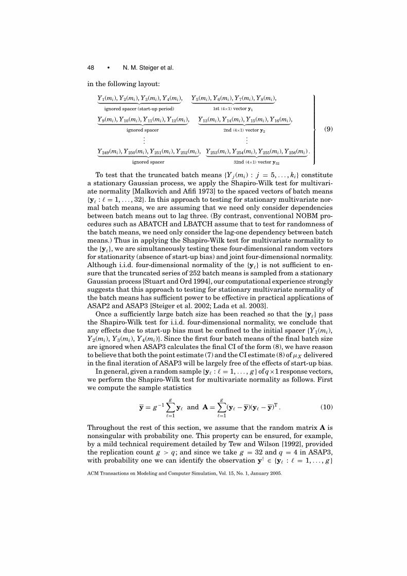
i = ki −4 = 252 denote the truncated count of batch means{Y j (mi) : j = 5, . . . , ki} that remain after skipping the first spacer, then we seethat ASAP3 builds 32 four-dimensional vectors {y� : � = 1, . . . , 32} as depicted
ACM Transactions on Modeling and Computer Simulation, Vol. 15, No. 1, January 2005.
48 • N. M. Steiger et al.
in the following layout:
Y1(mi), Y2(mi), Y3(mi), Y4(mi)︸ ︷︷ ︸ignored spacer (start-up period)
, Y5(mi), Y6(mi), Y7(mi), Y8(mi)︸ ︷︷ ︸1st (4×1) vector y1
,
Y9(mi), Y10(mi), Y11(mi), Y12(mi)︸ ︷︷ ︸ignored spacer
, Y13(mi), Y14(mi), Y15(mi), Y16(mi)︸ ︷︷ ︸2nd (4×1) vector y2
,
......
Y249(mi), Y250(mi), Y251(mi), Y252(mi)︸ ︷︷ ︸ignored spacer
, Y253(mi), Y254(mi), Y255(mi), Y256(mi)︸ ︷︷ ︸32nd (4×1) vector y32
.
(9)
To test that the truncated batch means {Y j (mi) : j = 5, . . . , ki} constitutea stationary Gaussian process, we apply the Shapiro-Wilk test for multivari-ate normality [Malkovich and Afifi 1973] to the spaced vectors of batch means{y� : � = 1, . . . , 32}. In this approach to testing for stationary multivariate nor-mal batch means, we are assuming that we need only consider dependenciesbetween batch means out to lag three. (By contrast, conventional NOBM pro-cedures such as ABATCH and LBATCH assume that to test for randomness ofthe batch means, we need only consider the lag-one dependency between batchmeans.) Thus in applying the Shapiro-Wilk test for multivariate normality tothe {y�}, we are simultaneously testing these four-dimensional random vectorsfor stationarity (absence of start-up bias) and joint four-dimensional normality.Although i.i.d. four-dimensional normality of the {y�} is not sufficient to en-sure that the truncated series of 252 batch means is sampled from a stationaryGaussian process [Stuart and Ord 1994], our computational experience stronglysuggests that this approach to testing for stationary multivariate normality ofthe batch means has sufficient power to be effective in practical applications ofASAP2 and ASAP3 [Steiger et al. 2002; Lada et al. 2003].
Once a sufficiently large batch size has been reached so that the {y�} passthe Shapiro-Wilk test for i.i.d. four-dimensional normality, we conclude thatany effects due to start-up bias must be confined to the initial spacer {Y1(mi),Y2(mi), Y3(mi), Y4(mi)}. Since the first four batch means of the final batch sizeare ignored when ASAP3 calculates the final CI of the form (8), we have reasonto believe that both the point estimate (7) and the CI estimate (8) of µX deliveredin the final iteration of ASAP3 will be largely free of the effects of start-up bias.
In general, given a random sample {y� : � = 1, . . . , g} of q×1 response vectors,we perform the Shapiro-Wilk test for multivariate normality as follows. Firstwe compute the sample statistics
y = g−1g∑
�=1
y� and A =g∑
�=1
(y� − y)(y� − y)T . (10)
Throughout the rest of this section, we assume that the random matrix A isnonsingular with probability one. This property can be ensured, for example,by a mild technical requirement detailed by Tew and Wilson [1992], providedthe replication count g > q; and since we take g = 32 and q = 4 in ASAP3,with probability one we can identify the observation y† ∈ {y� : � = 1, . . . , g}ACM Transactions on Modeling and Computer Simulation, Vol. 15, No. 1, January 2005.

ASAP3: A Batch Means Procedure for Steady-State Simulation Analysis • 49
for which
(y† − y)TA−1(y† − y) = max�=1,..., g
{(y� − y)TA−1(y� − y)}. (11)
We compute Z � ≡ (y† − y)TA−1(y� − y) for � = 1, . . . , g ; and we sort these auxil-iary quantities in ascending order to obtain the corresponding order statisticsZ (1) < · · · < Z (g ). Let {β� : � = 1, . . . , g} denote the associated coefficients ofthe univariate Shapiro-Wilk statistic for a random sample of size g as definedin Royston [1982a, 1982b]. Thus on the ith iteration of ASAP3 that requiresthe stationary multivariate normality test of step [2] as depicted in Figure 2,the null hypothesis Hmvn of i.i.d. four-dimensional normal responses {y�} is re-jected at the level of significance δi (0 < δi < 1) if the multivariate Shapiro-Wilkstatistic,
W ∗i =
[g∑
�=1
β�Z (�)
]2 /(y† − y)TA−1(y† − y), (12)
satisfies W ∗i < w∗
δi(q, g ), the δi quantile of the null distribution of W ∗
i . Thenull distribution of W ∗
i is the cumulative distribution function (c.d.f.) FW ∗ (·) of(12) when this statistic is based on a random sample of size g taken from aq-dimensional nonsingular normal distribution.
An additional iteration of ASAP3 will be required if the multivariate Shapiro-Wilk test yields a significant result (that is, the {y�} fail the test for i.i.d. four-dimensional normality) at the level of significance δi, where we take
δi = δ1 exp[−ω(i − 1)2] if i is a positive integer, (13)
with δ1 = 0.10, and ω = 0.18421. If the test statistic W ∗i computed from (12) on
iteration i corresponds to a P -value FW ∗ (W ∗i ) < δi, then in step [2] of ASAP3
as depicted in Figure 2, we update the iteration counter, the batch count, thetruncated batch count, the batch size, and the overall sample size according to
i ← i + 1, ki ← 256, k′i ← ki − 4, mi ← �√2mi−1�, and ni ← kimi, (14)
respectively. Thus on the next iteration of ASAP3 with the updated value ofthe iteration index i, the user must provide to the procedure the additionalsimulation responses {X j : j = ni−1 + 1, . . . , ni} so that ASAP3 can recomputethe ki batch means with the new batch size mi and then retest the k′
i truncatedbatch means for stationary multivariate normality.
The testing scheme described in (9)–(14) is specifically designed so that bothASAP2 and ASAP3 avoid the excessive variability in the final sample size thatwe have sometimes observed when ASAP is applied to simulation-generatedoutput processes with highly nonnormal marginals and no precision require-ment is specified. Equation (13) implies that for i = 1, . . . , 6, the significancelevel δi for the stationary multivariate normality test has the following values:0.10, 0.083, 0.048, 0.019, 0.0052, and 0.001, respectively; and on each iterationi beyond the sixth, δi declines by at least an order of magnitude. We formulatedthis testing scheme with the following objectives:
(a) We sought to compensate for the dependence between the outcomes onsuccessive iterations of the multivariate Shapiro-Wilk test in a single
ACM Transactions on Modeling and Computer Simulation, Vol. 15, No. 1, January 2005.

50 • N. M. Steiger et al.
application of ASAP3 so as to avoid an excessive overall probability of com-mitting a type I error—that is, falsely rejecting the hypothesis Hmvn thatthe batch means possess a four-dimensional normal distribution on someiteration of ASAP3 when the procedure is applied to a single simulationoutput process.
(b) We sought to impose an effective upper limit of about 20 on the number ofiterations of the multivariate Shapiro-Wilk test in a single application ofASAP3.
In routine applications of ASAP3, we have found that this testing scheme gener-ally requires 3–12 iterations of the Shapiro-Wilk test for i.i.d. four-dimensionalnormality. On the other hand, in processes with highly nonnormal marginals(such as the “AR(1)-to-Pareto,” or ARTOP, process discussed in Section 4.2.2),this scheme can require as many as 15 iterations of the multivariate Shapiro-Wilk test. Although the final batch means delivered by this testing schememay exhibit nonnegligible departures from multivariate normality, in practicewe have found a resultant degree of convergence to approximate multivariatenormality that is sufficient to yield acceptable overall performance of ASAP3 ina broad diversity of applications for which no precision requirement is specified.Clear evidence of this can be found in Section 4, especially in the experimentalresults for the M/M/1 queue waiting time process and the ARTOP process.Moreover, when a precision requirement is specified for ASAP3, in practice wehave found that the testing scheme (9)–(14) has much less impact on the per-formance of the overall procedure in terms of the final required sample size orthe properties of the final delivered CI.
3.2 Building an AR(1) Model for Stationary Multivariate Normal Batch Means
If the batch means pass the test for stationary multivariate normality on it-eration i of ASAP3, then we seek to adjust the conventional CI (3) for any re-maining correlations among the k′
i truncated batch means of the current batchsize mi by taking into account the extent to which those correlations causethe distribution of the classical NOBM t-ratio (5) to deviate from Student’st-distribution with k′
i − 1 degrees of freedom. Our adjustment is based on aninverse Cornish-Fisher expansion for the NOBM t-ratio that involves its firstfour cumulants. In the next section, we develop expressions for these cumulantsin terms of Var[Y j (mi)] and Var[ Y (mi, k′
i) ]. To compute sample estimators ofVar[Y j (mi)] and Var[ Y (mi, k′
i) ], we fit an AR(1) time series model (4) to thetruncated batch means {Y j (mi) : j = 5, . . . , ki}. For the batch means varianceestimator Var[Y j (mi)], we take the usual maximum likelihood estimator (MLE)of the variance of the fitted AR(1) process [Box et al. 1994]; and for the estimatorVar[Y (mi, k′
i)] of the variance of the truncated grand mean, we derive a similarstatistic based on the estimated covariances between all relevant batch meansexpressed in terms of the MLEs of the parameters of the fitted AR(1) process.
On the ith iteration of step [3] of ASAP3, the use of an AR(1) time seriesmodel (4) to represent the behavior of the truncated batch means is based onall our previous computational experience with ASAP and ASAP2. Although
ACM Transactions on Modeling and Computer Simulation, Vol. 15, No. 1, January 2005.

ASAP3: A Batch Means Procedure for Steady-State Simulation Analysis • 51
the original ASAP algorithm was equipped to fit more general autoregressive–moving average time series models to the batch means, for every application ofASAP in which the batch means had first passed the Shapiro-Wilk test for four-dimensional normality, the simple AR(1) model (4) fitted to the batch meansexhibited no significant lack of fit as well as the best fit of all the time se-ries models tested. We observed this behavior in all applications of ASAP in awide variety of test problems, including discrete-time Markov chains, queue-ing networks, inventory systems, and autoregressive processes. The responsesgenerated by these systems exhibited various autocorrelation structures andmarginal distributions that are encountered in practice [Steiger 1999; Steigerand Wilson 1999, 2000, 2002a]. This computational experience is the basis forthe fundamental assumption underlying the development of ASAP3—namely,that a batch size sufficient to induce approximate four-dimensional normalityin the batch means is also sufficient to ensure the adequacy of the AR(1) model(4) as an approximate representation of the stochastic behavior of the corre-sponding batch means. In general, identification and estimation of standardtime series models should be based on at least 50, and preferably 100 or moreobservations (see p. 17, Box et al. [1994]); and this is one of the reasons that step[3] of ASAP3 requires a truncated batch count of k′
i ≥ 252 on every iteration ofthe procedure.
If the truncated batch means {Y j (mi) : j = 5, . . . , ki} for batches of size miconstitute a stationary AR(1) process, then it follows from (4) that the batchmeans variance is given by Var[Y j (mi)] = Var[Y�] = σ 2
a /(1 − ϕ2), and moregenerally, the lag-q covariance between batch means for batches of size mi isgiven by
γY (mi )(q) ≡ Cov[Y j (mi), Y j+q(mi)] = ϕ|q|σ 2
a
/(1 − ϕ2) for q = 0, ±1, . . . ; (15)
see Section 3.2.3 of Box et al. [1994]. It also follows from (4) that
Var[Y (mi, k′i)] = 1
k′i
k′i−1∑
q=−k′i+1
(1 − |q|/k′i)γY (mi )
(q). (16)
Thus the batch means variance estimator Var[Y j (mi)] is obtained by insertingthe usual MLEs ϕ and σ 2
a of the respective parameters ϕ and σ 2a into (15) and
taking q = 0. The estimator Var[Y (mi, k′i)] of the variance of the truncated
grand mean is similarly obtained by inserting ϕ and σ 2a first into (15), and then
inserting the resulting estimated covariances into (16).When building an AR(1) model (4) of the truncated batch means, we have
found that we must avoid situations in which the MLE ϕ for the autoregressiveparameter ϕ is so close to one as to induce gross instability in the correlation-adjusted CI (6) based on the estimators ϕ, σ 2
a , Var[Y j (mi)], and Var[Y (mi, k′i)]. In
particular, we have found that if the lag-one correlation of the batch means (thatis, the correlation between adjacent batch means) substantially exceeds 0.8,then in the no precision case, CIs delivered by ASAP or ASAP2 can be extremelyunstable, with excessive values for the mean, variance, or coefficient of variationof the CI half-lengths. Experimental evidence of this phenomenon can be foundin Steiger and Wilson [1999, 2000, 2002a], Steiger et al. [2002], and Lada et al.
ACM Transactions on Modeling and Computer Simulation, Vol. 15, No. 1, January 2005.

52 • N. M. Steiger et al.
[2003]. A theoretical explanation for this phenomenon is detailed in AppendixA, where we also provide some evidence that ASAP3 delivers reasonably stableCIs if the batch size mi is taken sufficiently large to ensure that
Corr[Y j (mi), Y j+1(mi)] = ϕ ≤ 0.8. (17)
To test the hypothesis that ϕ meets condition (17) at the level of significanceαarp = 0.01, we seek a one-sided CI for ϕ that is based on ϕ and that, withprobability no less than 1 − αarp = 0.99, falls at or below the limit 0.8 when(17) holds. If the truncated batch means {Y j (mi) : j = 5, . . . , ki} constitute anAR(1) process (4), then it follows from Theorem 8.2.2 of Fuller [1996] that theautoregressive parameter estimator ϕ has the asymptotic distribution√
k′i (ϕ − ϕ)
D−→k′
i→∞ N(0, 1 − ϕ2). (18)
Unfortunately, it is well known that the convergence to normality in (18) canbe very slow when ϕ is close to one. In particular, Figure 8.2.1 of Fuller [1996]clearly reveals the nonnormality of ϕ for the sample size of 100 with ϕ = 0.9.
Applying the delta method [Stuart and Ord 1994] to (18), we propose usingthe arc sine transformation of ϕ,
S = sin−1(ϕ), (19)
to test for the condition (17). From (18) and Corollary A.14.17 of Bickel andDoksum [1977], we obtain the asymptotic property√
k′i[sin−1(ϕ) − sin−1(ϕ)]
D−→k′
i→∞ N (0, 1). (20)
Thus when k′i is large, sin−1(ϕ) is approximately normal with mean sin−1(ϕ) and
variance 1/k′i. In the case of an AR(1) process with mean zero (or, equivalently,
a known mean), Jenkins [1954] proposed taking the arc sine transformation ofthe circular serial correlation of lag one in which the sample mean is replacedby the known mean. Although in our situation the mean µX of the target AR(1)process (4) is unknown, and we are taking the arc sine transformation (19) ofthe maximum likelihood estimator ϕ of the autoregressive parameter ϕ, it isnot surprising that sin−1( ϕ ) and Jenkins’s statistic have similar asymptoticproperties; see p. 405 of Fuller [1996]. Jenkins recommended using the arcsine transformation when ϕ < 0.9; and this is further evidence supporting thecondition (17) required in ASAP3. Thus we chose to base step [3] of ASAP3 onthe statistic sin−1(ϕ).
Since k′i ≥ 252 on every iteration of ASAP3, we use the approximation
sin−1(ϕ)∼N [sin−1 (ϕ), 1/
k′i]
to test the hypothesis (17) at the level of significance αarp = 0.01 by checking forthe condition that the 100(1−αarp)% upper confidence limit for sin−1(ϕ) does notexceed the threshold sin−1(0.8) = 0.927. If on iteration i of step [3] of ASAP3we find
sin−1(ϕ) + z1−αarp /√
k′i ≤ sin−1(0.8) ⇐⇒ ϕ ≤ sin(0.927 − z1−αarp /
√k′
i) (21)
ACM Transactions on Modeling and Computer Simulation, Vol. 15, No. 1, January 2005.

ASAP3: A Batch Means Procedure for Steady-State Simulation Analysis • 53
(with z1−αarp = z0.99 = 2.33), then we conclude that the current batch size misatisfies (17) and we should proceed to the construction of a correlation-adjustedCI for µX in step [4] of ASAP3.
If the condition (21) is not satisfied, then in step [3] of ASAP3 we computethe required batch-size multiplier (inflation factor), and we update the iterationcounter, the batch count, the truncated batch count, the batch size, and theoverall sample size according to
θ ← mid{√2, ln[sin(0.927 − z1−αarp /√
k′i)]/ ln(ϕ), 4},
i ← i + 1, ki ← ki−1, k′i ← ki − 4, mi ← θmi−1�, and ni ← kimi,
}(22)
respectively. The basis for the batch-size multiplier θ in (22) is detailed inAppendix B. Thus on the next iteration of ASAP3 with the updated value of theiteration index i, the user must provide to the procedure the additional simula-tion responses {X j : j = ni−1 + 1, . . . , ni} so that ASAP3 can recompute the kibatch means with the new batch size mi, and then retest the hypothesis (17).
3.3 Confidence Interval Based on Batch Means Forming an AR(1) Process
Throughout most of this section, we suppress the iteration index i to simplifythe notation. No confusion should result from this usage since the iterationindex remains the same throughout this section. We formulate an adjustmentto the classical NOBM CI (3) that accounts for dependency between normalbatch means. The adjustment is based on the first four cumulants of the usualNOBM t-ratio,
t = Y (m, k′) − µX√S2
m,k′/k′= N
D, where
N ≡
√k′[Y (m, k′) − µX ]√
Var[Y (m)],
D ≡√
S2m,k′
Var[Y (m)],
(23)
on which the classical CI (3) is built. To simplify the discussion, we let N andD, respectively, denote the numerator and denominator of the t-ratio as in-dicated in (23). To compute the moments of (23), we make the following keyassumptions.
Assumption 1. The truncated batch means {Y j (m) : j = 5, . . . , k} have ajoint multivariate normal distribution.
Assumption 2. As defined in (23), the numerator N and denominator D ofthe NOBM t-ratio are independent.
Assumption 3. The squared denominator D2 of the t-ratio (23) is dis-tributed as χ2
νeff/νeff, where νeff = �2E2[S2
m,k′ ]/Var[S2m,k′ ]� denotes the effective
degrees of freedom associated with S2m,k′ .
Notice that if Assumption 1 holds and the batch means are independent,then Assumption 2 holds and Assumption 3 follows with νeff = k′ − 1. The
ACM Transactions on Modeling and Computer Simulation, Vol. 15, No. 1, January 2005.
54 • N. M. Steiger et al.
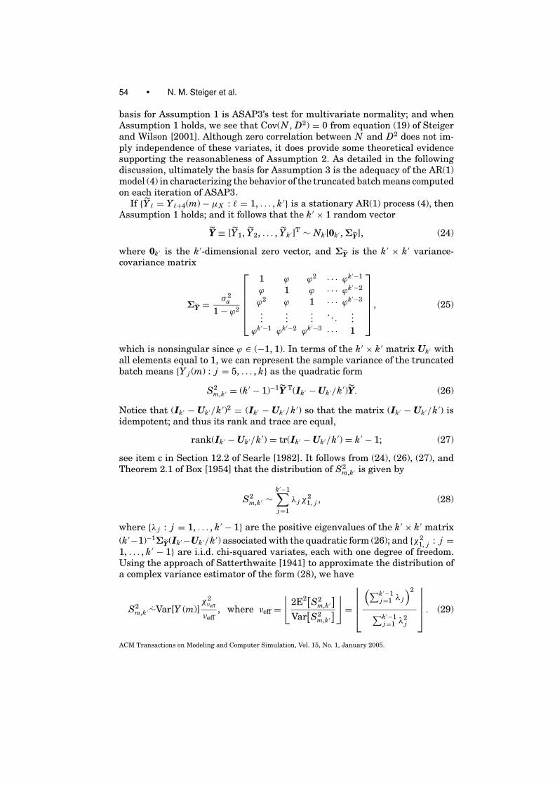
basis for Assumption 1 is ASAP3’s test for multivariate normality; and whenAssumption 1 holds, we see that Cov(N , D2) = 0 from equation (19) of Steigerand Wilson [2001]. Although zero correlation between N and D2 does not im-ply independence of these variates, it does provide some theoretical evidencesupporting the reasonableness of Assumption 2. As detailed in the followingdiscussion, ultimately the basis for Assumption 3 is the adequacy of the AR(1)model (4) in characterizing the behavior of the truncated batch means computedon each iteration of ASAP3.
If {Y� = Y�+4(m) − µX : � = 1, . . . , k′} is a stationary AR(1) process (4), thenAssumption 1 holds; and it follows that the k′ × 1 random vector
Y ≡ [Y1, Y2, . . . , Yk′ ]T ∼ Nk′[0k′ , ΣY], (24)
where 0k′ is the k′-dimensional zero vector, and ΣY is the k′ × k′ variance-covariance matrix
ΣY = σ 2a
1 − ϕ2
1 ϕ ϕ2 · · · ϕk′−1
ϕ 1 ϕ · · · ϕk′−2
ϕ2 ϕ 1 · · · ϕk′−3
......
.... . .
...ϕk′−1 ϕk′−2 ϕk′−3 · · · 1
, (25)
which is nonsingular since ϕ ∈ (−1, 1). In terms of the k′ × k′ matrix Uk′ withall elements equal to 1, we can represent the sample variance of the truncatedbatch means {Y j (m) : j = 5, . . . , k} as the quadratic form
S2m,k′ = (k′ − 1)−1Y T(Ik′ − Uk′/k′)Y. (26)
Notice that (Ik′ − Uk′/k′)2 = (Ik′ − Uk′/k′) so that the matrix (Ik′ − Uk′/k′) isidempotent; and thus its rank and trace are equal,
rank(Ik′ − Uk′/k′) = tr(Ik′ − Uk′/k′) = k′ − 1; (27)
see item c in Section 12.2 of Searle [1982]. It follows from (24), (26), (27), andTheorem 2.1 of Box [1954] that the distribution of S2
m,k′ is given by
S2m,k′ ∼
k′−1∑j=1
λ j χ21, j , (28)
where {λ j : j = 1, . . . , k′ − 1} are the positive eigenvalues of the k′ × k′ matrix(k′−1)−1ΣY(Ik′ −Uk′/k′) associated with the quadratic form (26); and {χ2
1, j : j =1, . . . , k′ − 1} are i.i.d. chi-squared variates, each with one degree of freedom.Using the approach of Satterthwaite [1941] to approximate the distribution ofa complex variance estimator of the form (28), we have
S2m,k′ ∼Var[Y (m)]
χ2νeff
νeff, where νeff =
⌊2E2[S2
m,k′]
Var[S2
m,k′]⌋
=
(∑k′−1
j=1 λ j
)2
∑k′−1j=1 λ2
j
. (29)
ACM Transactions on Modeling and Computer Simulation, Vol. 15, No. 1, January 2005.

ASAP3: A Batch Means Procedure for Steady-State Simulation Analysis • 55
Numerical evidence of the accuracy of the approximation (29) can be found inSatterthwaite [1941, 1946], Box [1954], and Welch [1956].
From Assumptions 1, 2, and 3, it follows that the first four cumulants of thet-ratio (23) are given by the following expressions:
κp = 0 for p = 1, 3 and νeff ≥ 5, (30)
κ2 = k′νeffVar[Y (m, k′)](νeff − 2)Var[Y (m)]
for νeff ≥ 4, (31)
κ4 = 6(k′)2ν2effVar2[Y (m, k′)]
(νeff − 2)2(νeff − 4)Var2[Y (m)]for νeff ≥ 6. (32)
See Steiger [1999] or Steiger and Wilson [2002a] for the details of the approachused to derive (30)–(32). In terms of these cumulants, we obtain the adjustedCI given by (6) from the inverse Cornish-Fisher expansion (6.56) of Stuart andOrd [1994] based on a standard normal density.
Remark 1. Notice that the leading coefficient in (32) is 6 rather than theleading coefficient of 2 that we find in equation (16) of Steiger et al. [2002]. Inthis respect, equation (16) of Steiger et al. [2002] is incorrect. Moreover, thesame error also occurs in equation (20) of Steiger and Wilson [2002a], whichshould actually read as follows:
κ4 = µ4 − 3µ22 = 6(k′)2(k′ − 1)2Var2[Y (m, k′)]
(k′ − 3)2(k′ − 5)Var2[Y (m)]for k′ ≥ 6.
It is also noteworthy that this error does not affect the operation of the ASAPsoftware [Steiger and Wilson 2002b], which is based on a different computa-tional formula for κ4 that is equivalent to the correct expression. Notice finallythat the correct versions of equations (15) and (16) in Steiger et al. [2002] canbe recovered if in (31) and (32) we replace every occurrence of νeff with k′ − 1.
The foregoing development suggested a modification of ASAP2 to take ex-plicit account of (29). We insert into (25) the MLEs ϕ and σ 2
a obtained by fit-ting the AR(1) model (4) to the truncated batch means, yielding the estimatorΣY, which is nonsingular with probability one, since |ϕ| < 1 with probabil-ity one. It follows that the random matrix (k′ − 1)−1ΣY (Ik′ − Uk′/k′) has rankk′ − 1 with probability one; and thus we can compute the positive eigenvalues{λ j : j = 1, . . . , k′ − 1} of this random matrix so as to obtain the estimatedeffective degrees of freedom
νeff = max
(∑k′−1j=1 λ j
)2
∑k′−1j=1 λ2
j
, 6
. (33)
Notice that in (33), we have taken 6 as the lower limit for νeff to ensure theexistence of the first four moments of the associated t-ratio (23) under theassumption that the squared denominator D2 has νeff degrees of freedom.
ACM Transactions on Modeling and Computer Simulation, Vol. 15, No. 1, January 2005.

56 • N. M. Steiger et al.
In comparison with the performance of ASAP2 for which the effective de-grees of freedom in D2 is always assumed (incorrectly) to be νeff = k′ − 1, wefound that the performance of ASAP3 was only slightly affected by (correctly)estimating νeff according to (33) rather than taking νeff = νeff = k′ − 1. Thus, weconcluded that the performance of the correlation-adjusted CI (6) is insensitiveto moderate errors in the determination of νeff. For this reason, and since nu-merical evaluation of the eigenvalues of a k′ ×k′ matrix can be computationallyintensive when 252 ≤ k′ ≤ 1,502, we use a two-dimensional array (table) ofprecalculated estimates of νeff in the production version of the ASAP3 software[Steiger et al. 2003]. We compiled this 26 × 19 table by varying k′ from 252 to1,502 in increments of 50 and by varying ϕ from −0.9 to 0.9 in increments of0.1; and then we computed the corresponding value of νeff for each of the 494combinations (k′, ϕ).
Thus, on the ith iteration of ASAP3 with truncated batch count k′i and au-
toregressive parameter estimator ϕ, the procedure searches the table of precal-culated estimates of νeff for (i) the tabled value of ϕ closest to the estimate ϕ
from the current AR(1) fit; and (ii) the tabled value of k′ closest to the truncatedbatch count k′
i for the current iteration of ASAP3. Then we take the estimatedeffective degrees of freedom νeff for the current iteration of ASAP3 to be thecorresponding value of νeff in the table; and we use this value for νeff in step [4]of ASAP3 to compute the estimates of the cumulants (30)–(32) for the t-ratio(23). Finally we insert into (6) the resulting cumulant estimators κ2 and κ4,along with the variance estimators Var [Y (m)] and Var [Y (m, k′)] described inSection 3.2, so as to obtain the approximate 100(1 − α)% CI for µX .
Remark 2. By design, we always have k′ ≥ 252; and the test condition (21)ensures that ϕ ≤ 0.80 on each iteration for which ASAP3 constructs a CI ofthe form (6). If we also have ϕ ≥ −0.80, then (33) implies νeff ≥ 55 so thatthe resulting CI is based on at least 55 effective degrees of freedom. In all ourexperimentation with ASAP3 on a wide range of types of stochastic systems, wehave found that νeff ≥ 55 for every CI constructed by ASAP3. This observationprovides another perspective on the relative stability of the final CIs deliveredby ASAP3.
3.4 Fulfilling the Precision Requirement
On the ith iteration of ASAP3, the final step [5] of the procedure is to determinewhether the constructed CI (6) with midpoint Y (mi, k′
i) and half-length H sat-isfies the user’s precision requirement. If the relevant user-specified precisionrequirement,
H ≤ H∗ (34)
=
∞, for no precision specification,r∗∣∣Y (mi, k′
i)∣∣ , for a relative precision specification,
max. acceptable CI half-length, for an absolute precision specification,
is satisfied, then ASAP3 terminates, returning a CI with midpoint Y (mi, k′i) and
half-length H. If the precision requirement (34) is not satisfied on iteration
ACM Transactions on Modeling and Computer Simulation, Vol. 15, No. 1, January 2005.

ASAP3: A Batch Means Procedure for Steady-State Simulation Analysis • 57
i of ASAP3, then the procedure estimates the number of additional batchesrequired to satisfy (34) using the current batch size mi,
k′′ = max{ (H/H∗)2k′i� − k′
i, 1}.To simplify the operation of ASAP3, we specified an admittedly arbitrary
upper limit on the number of batches that the algorithm may require. Pre-liminary experiments with ASAP3 revealed that no substantial improvementsin the performance of the procedure could be achieved by setting the upperlimit on the batch count much above 1,500. If the projected total numberof batches ki + k′′ ≤ 1,504, then we update the iteration counter, the batchcount, the truncated batch count, the batch size, and the total sample sizeaccording to
i ← i + 1, ki ← ki−1 + k′′, k′i ← ki − 4, mi ← mi−1, and ni ← miki,
respectively, so that the batch size remains unchanged, but the batch count isincreased by the multiplier (H/H∗)2. Our experiments with ASAP2 indicatedthat in those situations requiring more than 1,504 batches to achieve the de-sired precision, we could generally obtain better performance (in terms of finalrequired sample size) by increasing the batch size rather than increasing thebatch count.
If the projected total number of batches ki + k′′ > 1,504, then we leave thebatch count unchanged on the next iteration of ASAP3, and we increase thebatch size by a multiplier that is projected to satisfy the precision requirementbased on an approximation to the (complicated) way in which the half-length Hof the confidence interval (6) depends on the batch size. To achieve the desiredCI half-length H∗ on the next iteration based on the CI half-length H achievedon the current iteration, we must increase the current batch size by a multiplierθ ≥ 1 that is the root of the nonlinear equation
θ(1 − ϕ θ
+)2 = (H/H∗)2( 1 − ϕ+)2, (35)
where ϕ+ = max{0, ϕ} is the positive part of ϕ, the current estimate ofthe lag-one correlation between batch means for batches of the current size.The basis for (35) is detailed in Appendix C. Notice that when ϕ is close tozero in magnitude, or is negative, then (35) reduces to the familiar batch-sizemultiplier
θ = (H/H∗)2 (36)
that is usually recommended when the batch count is fixed and the batch sizeis already sufficiently large so that the batch means are approximately uncor-related (see, for example, Section 6.4.3 of Welch [1983]). For the same reasonsoutlined in Appendix B, we constrain θ to lie between the limits
√2 and 4 to
avoid an excessive number of iterations of ASAP3 or an excessive total samplesize.
Thus if ki + k′′ > 1,504 in step [5] of the current iteration of ASAP3, thenwe update the batch-size multiplier, the iteration counter, the batch count, the
ACM Transactions on Modeling and Computer Simulation, Vol. 15, No. 1, January 2005.

58 • N. M. Steiger et al.
truncated batch count, the batch size, and the total sample size according to
θ ← mid(√
2, θ , 4), i ← i + 1, ki ← ki−1,k′
i ← ki − 4, mi ← θmi−1� , and ni ← miki,
respectively. In any case, on the next iteration of ASAP3 with the updated it-eration index i, the batch count ki will not exceed 1,504; and the user mustprovide the additional simulation responses {X j : j = ni−1 + 1, . . . , ni} be-fore the batch means can be updated and steps [2]–[5] of ASAP3 can bereperformed.
4. EXPERIMENTAL PERFORMANCE EVALUATION
To evaluate the performance of ASAP3 with respect to the coverage proba-bility of its CIs, the mean and variance of the half-length of its CIs, and itstotal sample size, we applied ASAP3 together with ABATCH [Fishman 1996;Fishman and Yarberry 1997; Fishman 1998] and ASAP2 [Steiger et al. 2002;Lada et al. 2003] to a large suite of test problems. The experimental designincludes some problems typically used to test simulation output analysis pro-cedures and some problems more closely resembling real-world applications.To demonstrate the robustness of ASAP3, we limit our discussion here tothree problems possessing characteristics that we believe will strain any out-put analysis procedure—namely, a substantial start-up bias; a pronounced,slowly decaying correlation structure; or markedly nonnormal marginal distri-butions (or a combination of these). The steady-state mean response is avail-able analytically for each of these test problems; thus we were able to evaluatethe performance of ABATCH, ASAP2, and ASAP3 in terms of actual versusnominal coverage probabilities for the CIs delivered by each of these proce-dures. Experimental results for the remaining test problems are not presentedhere because they contribute little additional insight into the relative perfor-mance of the algorithms. In fact, the results reported in Section 4.2.1 andSection 4.2.2 that follow represent, respectively, the worst cases of CI over-coverage and undercoverage that we have experienced in all our applications ofASAP3.
For each test problem to be simulated, we performed 400 independent repli-cations of each batch means procedure to construct nominal 90% and 95% CIsthat satisfied four different precision requirements:
(a) no precision requirement—that is, we continued the simulation of each testproblem until ASAP3 delivered a CI (8) after the procedure first passed thetest (12) for stationary multivariate normality of the batch means and sub-sequently passed the test (21) for acceptable correlation between adjacentbatch means as prescribed in (17), with no precision specification in thestopping rule (34);
(b) ±15% precision—that is, we continued the simulation of each test problemuntil ASAP3 delivered a CI (8) that satisfied the relative precision require-ment (34) with r∗ = 0.15;
ACM Transactions on Modeling and Computer Simulation, Vol. 15, No. 1, January 2005.
ASAP3: A Batch Means Procedure for Steady-State Simulation Analysis • 59
(c) ±7.5% precision—that is, we continued the simulation of each test problemuntil ASAP3 delivered a CI (8) that satisfied the relative precision require-ment (34) with r∗ = 0.075; and
(d) ±3.75% precision—that is, we continued the simulation of each test prob-lem until ASAP3 delivered a CI (8) that satisfied the relative precisionrequirement (34) with r∗ = 0.0375.
In addition to the experimentation using the ASAP3 algorithm, we performed400 independent replications of the ASAP2 algorithm under the same precisionrequirements (a)–(d). Recall that unlike ASAP3, ASAP2 does not include thetest (21) for acceptable correlation between adjacent batch means.
Since ABATCH lacks a method for determining sample size, we passed to thisprocedure the same data sets used by ASAP3. Based on all our computationalexperience with ASAP2 and ASAP3, we believe that the results that follow aretypical of the performance of ASAP2 and ASAP3 that can be expected in manypractical applications. On the other hand, ABATCH is a nonsequential proce-dure whose proper operation may require direct user intervention [Fishman1998]; and thus it is not clear that the following results exemplify the perfor-mance of ABATCH in practical applications. Nevertheless, we believe that theresults given provide an arguably fair basis for comparing the performance ofABATCH, ASAP2, and ASAP3.
Since each CI was replicated 400 times, the standard error of the coverage es-timator for CIs with nominal 90% coverage probability is approximately 1.5%;and for CIs with nominal 95% coverage probability, the standard error of thecoverage estimator is approximately 1.1%. As explained in the following section,this level of precision in the estimation of coverage probabilities turns out tobe sufficient to reveal significant differences in the performance of ASAP3 com-pared with that of ASAP2 and ABATCH in the test problems presented here.
4.1 Single-Server Queue
Table I summarizes the experimental performance of the procedures ABATCH,ASAP2, and ASAP3 when they were applied to the M/M/1 queue waitingtime process for a system with an empty-and-idle initial condition, an inter-arrival rate of 0.9 customers per-time-unit, and a service rate of 1 customerper-time-unit. In this system, the steady-state server utilization is 0.9, and thesteady-state expected waiting time in the queue is µX = 9 time units. This isa particularly difficult test problem for several reasons: (i) the magnitude ofthe start-up bias is substantial and decays relatively slowly; (ii) in steady-stateoperation the autocorrelation function of the waiting time process decays veryslowly with increasing lags; and (iii) in steady-state operation the marginal dis-tribution of waiting times has an exponential tail and is, therefore, markedlynonnormal. Because of these characteristics, we can expect slow convergence tothe classical requirement that the batch means are i.i.d. normal. This test prob-lem clearly reveals one of the principal advantages of the ASAP3 algorithm—namely, that ASAP3 does not rely on any test for independence of the batchmeans.
ACM Transactions on Modeling and Computer Simulation, Vol. 15, No. 1, January 2005.

60 • N. M. Steiger et al.
Table I. Performance of Batch Means Procedures for the M/M/1 Queue Waiting Time Processwith Traffic Intensity τ = 0.9 Based on 400 Independent Replications of Nominal 90% and 95%
Confidence Intervals
Nominal 90% CIs Nominal 95% CIsPrecision
Requirement ABATCH ASAP3 ASAP2 ABATCH ASAP3 ASAP2No precisionavg. sample size 31,181 22,554 31,181 22,554coverage 76.0% 87.5% 88.0% 81.8% 91.5% 90.3%avg. rel. precision 0.161 0.239 0.579 0.193 0.290 0.730avg. CI half-length 1.388 2.072 6.440 1.669 2.521 8.300var. CI half-length 0.112 0.348 167.000 0.164 0.535 350.000±15% precisionavg. sample size 103,742 93,374 140,052 126,839coverage 80.5% 91.0% 90.0% 87.8% 95.5% 94.5%avg. rel. precision 0.098 0.134 0.135 0.104 0.136 0.136avg. CI half-length 0.865 1.182 1.184 0.921 1.206 1.204var. CI half-length 0.020 0.026 0.025 0.023 0.020 0.020±7.5% precisionavg. sample size 287,568 281,022 382,958 382,040coverage 85.8% 89.5% 92.0% 92.3% 94.3% 96.0%avg. rel. precision 0.063 0.070 0.070 0.066 0.071 0.071avg. CI half-length 0.561 0.627 0.628 0.588 0.632 0.633var. CI half-length 0.005 0.002 0.002 0.005 0.002 0.002±3.75% precisionavg. sample size 969,011 943,498 1,341,522 1,331,887coverage 88.8% 89.5% 92.0% 93.3% 93.5% 95.5%avg. rel. precision 0.035 0.036 0.036 0.036 0.036 0.036avg. CI half-length 0.318 0.320 0.323 0.323 0.321 0.322var. CI half-length 0.001 4.4E−4 3.0E−4 0.001 3.8E−4 3.0E−4
As can be seen from Table I, ASAP3 outperformed ABATCH with respectto CI coverage for the first three precision requirements. As we demand moreprecision, we are of course forced to perform more sampling. For the precisionrequirement of ±3.75%, the three algorithms gave similar results. The resultsin Table I suggest that ABATCH will give satisfactory coverage if this proce-dure is supplied with an adequate amount of data; however, ABATCH providesno mechanism for determining the amount of data that should be used. Notethat no average sample sizes are shown in the tables for the ABATCH proce-dure since the same samples that were generated for ASAP3 were also suppliedto ABATCH—that is, on each replication of ASAP3 and ABATCH, these twoprocedures used exactly the same data set, whose size was determined by thestopping rule (34) of ASAP3. Table 2 of Steiger and Wilson [2002a] shows thatsimply adding an absolute- or relative-precision stopping rule to ABATCH willnot generally yield acceptable performance for this procedure. A desirable fea-ture of ASAP3 is that it usually determines a sample size sufficient to yieldacceptable results.
In the absence of a precision requirement, ASAP2-generated CIs were highlyvariable in half-length. Imposing the requirement that the lag-one correlationbetween the batch means must not significantly exceed 0.8 greatly reducedthe variability of the half-lengths of the CIs generated by ASAP3, as shown in
ACM Transactions on Modeling and Computer Simulation, Vol. 15, No. 1, January 2005.

ASAP3: A Batch Means Procedure for Steady-State Simulation Analysis • 61
Table II. Performance of Batch-Means Procedures for the AR(1) Process with µX = 100, X 0 = 0,ρ = 0.995, and σε = 1 Based on 400 Independent Replications of Nominal 90% and 95%
Confidence Intervals
Nominal 90% CIs Nominal 95% CIsPrecision
Requirement ABATCH ASAP3 ASAP2 ABATCH ASAP3 ASAP2No precisionavg. sample size 41,076 10,305 41,076 10,305coverage 87.8% 95.5% 100.0% 93.5% 98.8% 100.0%avg. rel. precision 0.019 0.023 0.922 0.023 0.028 1.392avg. CI half-length 1.854 2.325 90.558 2.245 2.825 136.509var. CI half-length 0.113 0.170 5,159.18 0.173 0.270 14,915.200±15% precisionavg. sample size 41,076 51,908 41,076 75,677coverage 87.8% 95.5% 96.3% 93.5% 98.8% 97.5%avg. rel. precision 0.019 0.023 0.034 0.023 0.028 0.033avg. CI half-length 1.854 2.325 3.338 2.245 2.825 3.319var. CI half-length 0.113 0.170 9.836 0.173 0.270 11.050±1.875% precisionavg. sample size 68,474 395,012 101,526 584,646coverage 88% 95.5% 92.8% 93.8% 99.3% 96%avg. rel. precision 0.014 0.018 0.0075 0.014 0.018 0.0075avg. CI half-length 1.404 1.763 0.751 1.359 1.770 0.751var. CI half-length 0.058 0.013 0.217 0.056 0.012 0.228±0.9375% precisionavg. sample size 213,826 985,026 254,920 1,178,736coverage 87.5% 94.3% 93.5% 93.5% 97.3% 97%avg. rel. precision 0.0077 0.0089 0.0047 0.0083 0.0090 0.0048avg. CI half-length 0.765 0.894 0.478 0.828 0.896 0.478var. CI half-length 0.017 0.0026 0.055 0.011 0.0021 0.057
Table I. Moreover, in terms of CI coverage, ASAP3 performed as well as ASAP2in the no precision case.
4.2 Processes Based on Autoregression
4.2.1 First-Order Autoregressive (AR(1)) Process. For a second test case,we chose an AR(1) process, given by
X � = µX + ρ(X �−1 − µX ) + ε� for � = 1, 2, . . . ,
where the white noise term ε� is an independent normal residual with meanzero and variance σ 2
ε . We set the mean µX = 100, the initial condition X 0 = 0,the autoregressive parameter ρ = 0.995, and white-noise variance σ 2
ε = 1.We designed this case to be a particularly difficult one in two main respects.First, there is a pronounced initial transient in each time series of simulation-generated observations from this process since we always take X 0 = 0. Second,the extremely high correlation provides a severe test of ASAP3’s method of cal-culating the cumulants of the t-ratio (23) and then constructing the correlation-adjusted CI (6) as described in Section 3.3. The results for this test problem aresummarized in Table II.
ACM Transactions on Modeling and Computer Simulation, Vol. 15, No. 1, January 2005.

62 • N. M. Steiger et al.
The selected AR(1) process most dramatically demonstrates the improve-ment in the performance of ASAP3 compared with that of ASAP2. In the noprecision case for this test problem, ASAP2 yielded highly variable CIs thatwere so wide as to be practically meaningless. The breakdown in the perfor-mance of ASAP2 is due to the batch means passing the test for stationary mul-tivariate normality at batch sizes for which the batch means remain stronglycorrelated, with both ϕ and ϕ substantially exceeding 0.8. The proximity of ϕ toone results in the condition of gross instability that is described in Section 3.2and in Appendix A, and that we seek to avoid in ASAP3 by progressively in-creasing the batch size until the condition (21) is satisfied so that the hypothesis(17) can be accepted.
Notice that for the precision requirement of ±15%, both ASAP2 and ASAP3actually delivered an average relative precision of at most 3.4%; and thus theresults for the precision requirements of ±7.5% and ±3.75% do not involve anysubstantial additional sampling for either procedure. To provide some indica-tion of the asymptotic performance as r∗ → 0 for ABATCH, ASAP2, and ASAP3when they are applied to the selected AR(1) process, in Table II we omitted theresults for the precision requirements of ±7.5% and ±3.75% and included in-stead the results for the precision requirements of ±1.875% and ±0.9375%.
Table II shows that while ASAP3 still experienced some overcoverage, its CIswere much better behaved than those of ASAP2. In the no precision case, theaverage half-lengths of the CIs delivered by ASAP3 were one to two orders ofmagnitude smaller than those for ASAP2; and the variances of the half-lengthsfor CIs delivered by ASAP3 were three to four orders of magnitude smaller thanthe corresponding quantities for ASAP2. For relative precision requirements of±1.875% and ±0.9375%, ASAP2 and ASAP3 delivered approximately the samecoverage probabilities; however, ASAP2 required substantially larger samplesizes than ASAP3 required. Moreover, ASAP3 delivered CIs whose levels of av-erage relative precision were close to the corresponding nominal levels (that is,±1.875% or ±0.9375%). On the other hand, ASAP2 delivered CIs whose levelsof average relative precision were substantially below the corresponding nom-inal levels. We believe that the superior performance of ASAP3 in these twocases is due to the bounding scheme (51) that is imposed on the batch-size mul-tiplier θ in step [5] of ASAP3, where we estimate the new batch size needed tosatisfy the precision requirement. This bounding scheme may force ASAP3 toperform more iterations than ASAP2 would perform to satisfy the same preci-sion requirement in some situations; but in our computational experience, (51)prevents the “runaway” sample sizes that are sometimes delivered by ASAP2to satisfy the precision requirement.
4.2.2 AR(1)-to-Pareto (ARTOP) Process. The next system used to test theperformance of ASAP3 was the “AR(1)-to-Pareto,” or ARTOP, process. If {X j :j = 1, 2, . . .} is an ARTOP process with marginal c.d.f.,
FX (x) ≡ Pr{X ≤ x} ={
1 − (ξ/
x)ψ , x ≥ ξ,
0, x < ξ,(37)
ACM Transactions on Modeling and Computer Simulation, Vol. 15, No. 1, January 2005.

ASAP3: A Batch Means Procedure for Steady-State Simulation Analysis • 63
where ξ > 0 is a location parameter and ψ > 0 is a shape parameter, then we cangenerate {X j } from a “base process” {Z j : j = 1, 2, . . .} that is a stationary AR(1)process with N (0, 1) marginals and lag-one correlation ρ. First, we generate thebase process {Z j : j = 1, 2, . . .} according to
Z j = ρZ j−1 + bj , (38)
where Z0 ∼ N (0, 1), and {bj : j = 1, 2, . . .}i.i.d.˜ N (0, σ 2
b ) is a white noise processwith variance σ 2
b = σ 2Z (1 −ρ2) = 1 −ρ2. Then, we feed the base process into the
standard normal c.d.f. to obtain a sequence of correlated, uniform(0,1) randomvariables {U j = �(Z j ) : j = 1, 2, . . .}, where
�(z) =∫ z
−∞
1√2π
e−w2/2dw for all real z
denotes the N (0, 1) c.d.f. Finally, we feed the process {U j : j = 1, 2, . . .} intothe inverse of the Pareto c.d.f. (37) to generate the ARTOP process {X j : j =1, 2, . . .} as follows,
X j = F −1X (U j ) = F −1
X [�(Z j )] = ξ/[1 − �(Z j )]1/ψ , j = 1, 2, . . . . (39)
The mean and the variance of the ARTOP process (39) are given by
µX = E[X j ] = ψξ (ψ − 1)−1, for ψ > 1,
and
σ 2X = Var[X j ] = ξ2ψ(ψ − 1)−2(ψ − 2)−1, for ψ > 2,
respectively [Johnson et al. 1994].We set the parameters of the Pareto distribution (37) according to ψ = 2.1 and
ξ = 1; and we set the lag-one correlation in the base process (38) to ρ = 0.995.This yielded an ARTOP process {X j : j = 1, 2, . . .} whose marginal distributionhas mean, variance, skewness, and kurtosis, respectively, given by
µX = 1.9091, σ 2X = 17.3554, E
[(X j − µX
σX
)3]
= ∞, and E
[(X j − µX
σX
)4]
= ∞.
The most difficult aspect of this system is that the marginals are highly non-normal, and their distribution has a very heavy tail. We sampled Z0 from theN (0, 1) distribution when generating the process {X j } so that the process be-gan in steady-state operation. Therefore, there was no start-up problem forthis process. The results obtained for the ARTOP process are summarized inTable III.
We can see from Table III that ASAP3 yielded some undercoverage in thisproblem. The reason for this minor undercoverage is that, even at substantialbatch sizes, the batch means are nonnormal. In fact, the batch means mostfrequently passed the test for stationary multivariate normality on iterationi = 9 of ASAP3. At this point in the operation of ASAP3, the significance level ofthe test (13) is given by δ9 = 7.6×10⁻⁶. In practical terms, the batch means haveessentially failed to converge to normality before ASAP3 proceeds to constructa CI. In spite of the remaining deviation of the batch means from normality, the
ACM Transactions on Modeling and Computer Simulation, Vol. 15, No. 1, January 2005.

64 • N. M. Steiger et al.
Table III. Performance of Batch-Means Procedures for the ARTOP Process Based on 400Independent Replications of Nominal 90% and 95% Confidence Intervals
Nominal 90% CIs Nominal 95% CIsPrecision
Requirement ABATCH ASAP3 ASAP2 ABATCH ASAP3 ASAP2No precisionavg. sample size 114,053 113,336 114,053 113,336coverage 82.8% 85.5% 85.8% 88.0% 90.8% 90.3%avg. rel. precision 0.083 0.091 0.093 0.100 0.109 0.112avg. CI half-length 0.158 0.173 0.179 0.190 0.207 0.214var. CI half-length 0.006 0.010 0.012 0.009 0.014 0.018±15% precisionavg. sample size 117,092 117,883 120,660 121,015coverage 82.5% 85.5% 85.5% 88.00% 90.8% 90.5%avg. rel. precision 0.080 0.087 0.087 0.094 0.101 0.101avg. CI half-length 0.151 0.163 0.165 0.178 0.190 0.191var. CI half-length 0.002 0.002 0.003 0.002 0.002 0.003±7.5% precisionavg. sample size 186,517 183,534 255,512 252,741coverage 82.0% 84.0% 84.8% 90.5% 90.3% 90.3%avg. rel. precision 0.064 0.068 0.068 0.067 0.070 0.070avg. CI half-length 0.121 0.127 0.128 0.126 0.131 0.132var. CI half-length 3.0E−04 2.1E−04 2.0E−04 2.9E−04 1.2E−04 1.0E−04±3.75% precisionavg. sample size 814,486 730,168 1,057,153 1,042,711coverage 86.5% 87.3% 85.0% 93.3% 92.5% 91.3%avg. rel. precision 0.035 0.035 0.035 0.036 0.035 0.035avg. CI half-length 0.066 0.066 0.067 0.068 0.067 0.067var. CI half-length 4.5E−5 2.7E−5 2.4E−5 4.6E−5 2.6E−5 2.5E−5
correlation-adjusted CIs achieved nearly nominal coverage. We have found boththe ASAP2 and ASAP3 algorithms were relatively robust against nonnormalmarginals, and some deviation from normality did not cause the catastrophicloss of coverage with ASAP3 that we have sometimes experienced with otherNOBM procedures. The slowness of convergence to normality in this problemrequires sample sizes large enough to result in near nominal coverage fromABATCH as well.
4.3 Computational Complexity of ASAP3
The most computationally intensive portion of ASAP3 is the batching process,which runs in O(n) time and requires O(1) memory since data is passed toASAP3 via external files, and ASAP3 maintains, at most, 1,504 batch means inmemory. Moreover, since ASAP3 uses a bounded number of batches not only inthe test for normality but also in fitting an AR(1) model, the corresponding stepsof the procedure run in O(1) time and require O(1) memory. We eliminated thecomputationally intensive calculation of the effective degrees of freedom (33) byreturning this value from a table containing values corresponding to selectedAR(1) parameters and numbers of batches. It follows that each iteration ofASAP3 runs in O(n) time and requires O(1) memory.
ACM Transactions on Modeling and Computer Simulation, Vol. 15, No. 1, January 2005.

ASAP3: A Batch Means Procedure for Steady-State Simulation Analysis • 65
Beyond this characterization of the computational complexity of ASAP3, weremark that performing hundreds of replications of ASAP3 on many test prob-lems enabled us to observe the actual performance of ASAP3 in several thou-sand applications. The number of batching operations, and hence the actualcomputing time, was not onerous even in the most difficult cases. The othersteps of ASAP3—testing for normality, fitting an AR(1) model, and calculatingthe correlation-adjusted CI—require negligible computer time in practice.
5. CONCLUSIONS AND RECOMMENDATIONS
ASAP3 is based on the widely used and easily understood method of nonover-lapping batch means. Conventional application of this method requires thatthe batch size must be large enough to obtain approximately i.i.d. normal batchmeans. Prior to the introduction of ASAP, most batching schemes focused on de-termining a batch size and number of batches adequate to achieve approximateindependence of the batch means, under the assumption that such a configura-tion would be sufficient to result in approximate normality of the batch means.We designed the original ASAP algorithm on the premise that in the absenceof approximate independence of the batch means, the approximate joint mul-tivariate normality of the batch means will enable us to adjust the classicalNOBM CI for any dependence between the final batch means. Although theexperimental results for ASAP showed that this approach had promise, therewere instances of substantial undercoverage or overcoverage in some test prob-lems; and in some applications of ASAP that lacked a precision requirement,we observed excessive variability in ASAP’s required sample sizes and in thehalf-lengths of the final CIs. ASAP3 incorporates all the changes to ASAP andASAP2 that we developed to correct these performance deficiencies.
The undercoverage problem encountered with ASAP was largely eliminatedby removal of the test for independence of the batch means. Both ASAP2 andASAP3 test only for stationary multivariate normality of the batch means andalways deliver a CI adjusted for correlation, if any, among the final batch means.Excessive variabilities seen with ASAP in the final sample sizes, and to someextent in the final CI half-lengths, were partially resolved in ASAP2 by de-creasing the significance level of the test for stationary multivariate normalityon each iteration of that test. Moreover, the means and variances of the finalCI half-lengths delivered by ASAP3 were greatly reduced in comparison withthe corresponding quantities delivered by ASAP and ASAP2; and ASAP3 hasachieved this performance improvement by progressively increasing the batchsize until the estimator of the correlation between adjacent batch means doesnot exceed 0.8.
ASAP3 is primarily designed for use in conjunction with a user-specified ab-solute or relative precision requirement on the final CI; and when it is used inthis way, ASAP3 generally delivers CIs whose coverage probability is close tothe nominal level. Although ASAP3 does not provide a definitive resolution of allproblems associated with the batch means method for steady-state simulationoutput analysis, many of the undesirable behaviors of its predecessors, ASAP
ACM Transactions on Modeling and Computer Simulation, Vol. 15, No. 1, January 2005.
66 • N. M. Steiger et al.
and ASAP2, have been eliminated; and there is good evidence to show thatASAP3’s performance in practice compares favorably with other well-knownbatch means procedures. We believe the basic approach of ASAP3 has the po-tential to lead to new developments in the method of batch means.
There are several issues concerning ASAP3 that require further work. Thekey assumption underlying the development presented in this article is thatthe AR(1) process (4) provides an adequate model of the batch means after theyhave passed the multivariate Shapiro-Wilk test (9)–(14). We have substantialexperimental evidence that increasing the batch size improves the accuracyof the AR(1) fit to the corresponding batch means; and thus a possible exten-sion of ASAP3 would be to incorporate into step [3] of the procedure a formalsubprocedure to test the goodness of fit of the AR(1) model, if necessary in-creasing the batch size and repeating the goodness-of-fit test until the batchmeans finally pass that test. The results of Amemiya and Wu [1972] and Kangand Schmeiser [1987] on the effects of batching autoregressive–moving averagetime series may shed some light on the desirability of implementing such anextension of ASAP3. We are currently investigating this issue.
Because there is much less evidence for the approximate validity of Assump-tion 2 in Section 3.3 than for the approximate validity of Assumptions 1 and3 in general applications of ASAP3, another direction for future research is toundertake a careful examination of Assumption 2 and of the potential effectsof violations of this basic property on the performance of ASAP3.
The asymptotic properties of ASAP3 also require thorough examination. Atheoretical investigation should address the asymptotic validity of ASAP3’sCIs—that is, the actual coverage probability of CIs delivered by ASAP3 shouldconverge to the nominal level 1 − α as the precision specification (for example,r∗) tends to zero. We must also address the question of ASAP3’s asymptoticefficiency in the sense of Chow and Robbins [1965] and Nadas [1969]. We know,for example, that in the case of the M/M/1 queue waiting time process witharrival rate of 0.9 customers per-time-unit and service rate of 1 customer per-time-unit, the steady-state mean queueing time µX has the specific value 9time units, and the steady-state variance constant defined by
σ 2 ≡ limn→∞ nVar[X (n)] = lim
m→∞(mk)Var[Y (m, k)] (40)
has the specific value 35,901 (see, for example, Section 2 and Section 4.2 ofSteiger and Wilson [2001]). It follows from (40) that to deliver a 100(1 − α)%CI for µX with a relative precision of r∗, an efficient procedure (in the sense ofChow and Robbins [1965]) would require an expected total sample size of
n∗ = ⌈σ 2z2
1−α/2
/(r∗µX )2
⌉; (41)
and for the particular case of the given M/M/1 queue waiting time process inwhich α = 0.10 and r∗ = 0.075, we have from (41) that n∗ = 213,222. FromTable I we see that ASAP3 requires an average sample size of 287,568 for thiscase and delivers nearly nominal coverage—specifically, 89.5%. Thus to delivera nominal 90% confidence interval on the steady-state mean queueing timewith relative precision of ±7.5% in this particular system, ASAP3 appears to
ACM Transactions on Modeling and Computer Simulation, Vol. 15, No. 1, January 2005.

ASAP3: A Batch Means Procedure for Steady-State Simulation Analysis • 67
be relatively efficient. It is less clear how ASAP3 performs across a large class ofsteady-state simulation applications for values of r∗ commonly used in practiceas well as for the asymptotic case in which we let r∗ → 0.
Another area of future work includes continued testing of the ASAP3 algo-rithm on different types of stochastic systems. Suarez-Gonzalez et al. [2002]perform some testing of the original ASAP algorithm on long-range dependentprocesses. We would like to apply ASAP3 to these and other problems typicallyencountered in some telecommunications applications.
For the case of the ARTOP process in which the skewness and kurtosis ofthe marginal distribution are both infinite, the observed slippage in ASAP3’sCI coverage probabilities leads us to believe that perhaps some higher-ordermoment requirements are necessary for the proper application and function-ing of ASAP3. Future work should include investigation of possible requisitemoment conditions.
Additional experimental results, follow-up papers and revised software, willbe available on the website <www.ie.ncsu.edu/jwilson>.
APPENDIX
A. Basis for Relation (17)
If the series of batch means {Y j (m)} having length k′ constitutes a stationaryAR(1) process (4), then from (15) and (16) we have the asymptotic relation
limk′→∞
k′Var[Y (m, k′)]Var[Y (m)]
= 1 + ϕ
1 − ϕ. (42)
It follows from (42) that for k′ large, we have the following approximate expres-sions for the first four cumulants of the t-ratio (5) based on equations (30)–(32),which are derived in Section 3.3:
κp ≈ 0 for p = 1, 3; (43)
κ2 ≈ νeff
νeff − 2
(1 + ϕ
1 − ϕ
), (44)
κ4 ≈ 6ν2eff
(νeff − 4)(νeff − 2)2
(1 + ϕ
1 − ϕ
)2
= 6κ22
νeff − 4. (45)
It follows from (43)–(45) and equation (21) of Steiger and Wilson [2002a] thatfor k′ large, the ratio of the expected half-length of the correlation-adjusted CI(6) to the expected half-length of the classical NOBM CI (3) is approximatelygiven by
R ≈ 12
+ κ2
2− κ4
8+ κ4
24z2
1−α/2 (46)
= 12
+ νeff
2(νeff − 2)
(1 + ϕ
1 − ϕ
)+ 3ν2
eff
4(νeff − 4)(νeff − 2)2
(1 + ϕ
1 − ϕ
)2(
z21−α/2
3− 1
).
ACM Transactions on Modeling and Computer Simulation, Vol. 15, No. 1, January 2005.
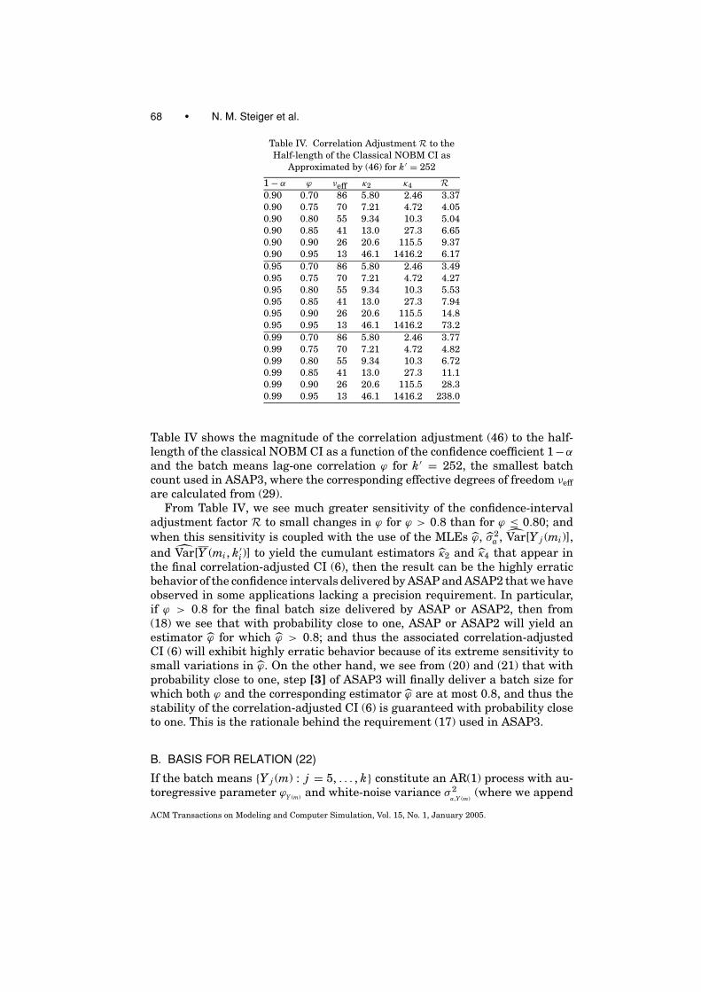
68 • N. M. Steiger et al.
Table IV. Correlation Adjustment R to theHalf-length of the Classical NOBM CI as
Approximated by (46) for k′ = 252
1 − α ϕ νeff κ2 κ4 R0.90 0.70 86 5.80 2.46 3.370.90 0.75 70 7.21 4.72 4.050.90 0.80 55 9.34 10.3 5.040.90 0.85 41 13.0 27.3 6.650.90 0.90 26 20.6 115.5 9.370.90 0.95 13 46.1 1416.2 6.170.95 0.70 86 5.80 2.46 3.490.95 0.75 70 7.21 4.72 4.270.95 0.80 55 9.34 10.3 5.530.95 0.85 41 13.0 27.3 7.940.95 0.90 26 20.6 115.5 14.80.95 0.95 13 46.1 1416.2 73.20.99 0.70 86 5.80 2.46 3.770.99 0.75 70 7.21 4.72 4.820.99 0.80 55 9.34 10.3 6.720.99 0.85 41 13.0 27.3 11.10.99 0.90 26 20.6 115.5 28.30.99 0.95 13 46.1 1416.2 238.0
Table IV shows the magnitude of the correlation adjustment (46) to the half-length of the classical NOBM CI as a function of the confidence coefficient 1−α
and the batch means lag-one correlation ϕ for k′ = 252, the smallest batchcount used in ASAP3, where the corresponding effective degrees of freedom νeffare calculated from (29).
From Table IV, we see much greater sensitivity of the confidence-intervaladjustment factor R to small changes in ϕ for ϕ > 0.8 than for ϕ ≤ 0.80; andwhen this sensitivity is coupled with the use of the MLEs ϕ, σ 2
a , Var[Y j (mi)],and Var[Y (mi, k′
i)] to yield the cumulant estimators κ2 and κ4 that appear inthe final correlation-adjusted CI (6), then the result can be the highly erraticbehavior of the confidence intervals delivered by ASAP and ASAP2 that we haveobserved in some applications lacking a precision requirement. In particular,if ϕ > 0.8 for the final batch size delivered by ASAP or ASAP2, then from(18) we see that with probability close to one, ASAP or ASAP2 will yield anestimator ϕ for which ϕ > 0.8; and thus the associated correlation-adjustedCI (6) will exhibit highly erratic behavior because of its extreme sensitivity tosmall variations in ϕ. On the other hand, we see from (20) and (21) that withprobability close to one, step [3] of ASAP3 will finally deliver a batch size forwhich both ϕ and the corresponding estimator ϕ are at most 0.8, and thus thestability of the correlation-adjusted CI (6) is guaranteed with probability closeto one. This is the rationale behind the requirement (17) used in ASAP3.
B. BASIS FOR RELATION (22)
If the batch means {Y j (m) : j = 5, . . . , k} constitute an AR(1) process with au-toregressive parameter ϕY (m) and white-noise variance σ 2
a,Y (m)(where we append
ACM Transactions on Modeling and Computer Simulation, Vol. 15, No. 1, January 2005.
ASAP3: A Batch Means Procedure for Steady-State Simulation Analysis • 69
to the symbols used in (4) the subscript Y (m) to emphasize the dependence onthe batch size m), then we seek to calculate the lag-q correlation between batchmeans for batches of size gm:
ρY (gm) (q) ≡ Corr[Y1(gm), Y1+q(gm)] for g = 1, 2, . . . , and q = 0, ±1, . . . ,
especially in the critical situation that ϕY (m) > 0.8. First we note that for eachpositive integer g and for q = 0, 1, 2, . . . , the lag-q covariance between batchmeans for batches of size gm is given by
Cov[Y1(gm), Y1+q(gm)] = Cov
[1g
g∑u=1
Yu(m),1g
g∑v=1
Y gq+v(m)
]
= 1g2
{g∑
u=1
g∑v=1
Cov[Yu(m), Y gq+v(m)]
}
= 1g2
[g∑
u=1
g∑v=1
σ 2a,Y (m)
ϕ gq+v−uY (m)
1 − ϕ2Y (m)
]by (15)
≥ 1g2
[g∑
u=1
g∑v=1
σ 2a,Y (m)
ϕ gq+|v−u|Y (m)
1 − ϕ2Y (m)
]
=σ 2
a,Y (m)ϕ gq
Y (m)
g[1 − ϕ2
Y (m)
][
1 + 2g−1∑u=1
(1 − u
g
)ϕu
Y (m)
]; (47)
and from (47), it follows immediately that
ρY (gm) (q) ≥ ϕ g |q|Y (m)
for g = 1, 2, . . . , and q = 0, ±1, . . . . (48)
Moreover, we have the following asymptotic relation as ϕY (m) tends to 1 from theleft,
ρY (gm) (q) ≈ ϕ g |q|Y (m)
for g = 1, 2, . . . , and q = 0, ±1, . . . as ϕY (m) → 1−; (49)
and, in practice, we have found that (49) provides a reasonably accurate ap-proximation in the situation that 0.8 < ϕY (m) < 1.
On the basis of (49), we postulate that the lag-one correlation between batchmeans for batches of size θm� is given approximately by
ρY ( θm�) (1) ≈ ϕθ
Y (m)for 0.8 < ϕY (m) < 1 and for all real θ ≥ 1. (50)
In practice, we have found that the approximation (50) is fairly accurate for1 ≤ θ ≤ 4 but that (50) is much less accurate for θ > 4. Moreover, we havefound that in some situations (50) yields a batch size that satisfies the constraint(21) with very little slack; and then on subsequent iterations of ASAP3, smallnoise-induced violations of (21) can result in an excessive number of relativelysmall increases in batch size that are required to restore the condition (21).To avoid not only excessive errors in the approximation (50) but also excessiveiterations of ASAP3 to adjust the batch size, we found empirically that θ shouldbe constrained to the interval √
2 ≤ θ ≤ 4. (51)
ACM Transactions on Modeling and Computer Simulation, Vol. 15, No. 1, January 2005.

70 • N. M. Steiger et al.
Combining (50) with (51) and (21), we see that if (21) is not satisfied withthe current batch size m, then we need to increase the batch size on the nextiteration of ASAP3 by the multiplier θ as specified in (22).
C. BASIS FOR RELATION (35)
It follows from (42)–(45) and equation (21) of Steiger and Wilson [2002a] thatfor k′ large, the half-length of the current CI based on k′ batches of size m isgiven by
H = z1−α/2
(12
+ κ2
2− κ4
8+ κ4
24z2
1−α/2
) √Var[Y (m)]
k′
≈ z1−α/2
[12
+ νeff
2(νeff − 2)
(1 + ϕ
1 − ϕ
)
+ 3ν2eff
4(νeff − 4)(νeff − 2)2
(1 + ϕ
1 − ϕ
)2(
z21−α/2
3− 1
) ]√σ 2
mk′ , (52)
where σ 2 ≡ mVar[Y (m)] is the current estimator of the steady-state varianceconstant σ 2 defined by (40) based on the sample variance estimator (16). Ifϕ ≤ 0, then the confidence interval (52) is no wider than the classical NOBMconfidence interval (3); and in this situation, we adopt the conservative ap-proach of assuming the current batch means are approximately independent.This is tantamount to using ϕ+ ≡ max{0, ϕ} in the following analysis of how(52) depends on the batch size.
In terms of the quantities
Q1 ≡ νeff
2(νeff − 2)
(1 + ϕ+1 − ϕ+
)and
Q2 ≡ 3ν2eff
4(νeff − 4)(νeff − 2)2
(1 + ϕ+1 − ϕ+
)2(
z21−α/2
3− 1
),
we see that
Q2
Q1= 3νeff
2(νeff − 4)(νeff − 2)
(1 + ϕ+1 − ϕ+
) (z2
1−α/2
3− 1
);
and since we always have νeff ≥ 55 and ϕ+ ≤ 0.8 in view of Remark 2, it followsthat
|Q2/Q1| ≤ 0.077 for α = 0.10, 0.05. (53)
On the basis of (53) and extensive computational experience with ASAP3 whichshows that in practice |Q2/Q1| rarely exceeds 0.02 and never exceeds 0.04, weconclude that
Q1 � Q2 (54)
in practical applications of ASAP3. Thus, we will neglect Q2 in the rest of theanalysis that follows.
ACM Transactions on Modeling and Computer Simulation, Vol. 15, No. 1, January 2005.
ASAP3: A Batch Means Procedure for Steady-State Simulation Analysis • 71
Now if we increase the batch size from m to θm� for θ ≥ 1, then from (52)and (54), we see that the resulting CI half-length will be approximately givenby
H(θ ) ≈ z1−α/2
[12
+ νeff
2(νeff − 2)
(1 + ϕ θ
+1 − ϕ θ+
)] √σ 2
θmk′ ;
and it follows that for large νeff, we have νeff/(νeff − 2) ≈ 1 and
H(θ )/H ≈ (1 − ϕ+)/[(
1 − ϕ θ+)√
θ].
Thus to achieve acceptable precision, we must set θ such that
H(θ ) = H∗ ⇐⇒ θ(1 − ϕ θ
+)2 = (H/H∗)2( 1 − ϕ+)2;
and this establishes (35).
Remark 3. It is easy to see that a lower bound on the solution to (35) isgiven by
θ ′ = (H/H∗)2(1 − ϕ+)2; (55)
and an upper bound can be obtained from (55) as follows,
θ ′′ = (H/H∗)2[(1 − ϕ+)/(
1 − ϕ θ ′+
)]2. (56)
Equations (55) and (56) can provide the starting points for standard numericalmethods of solving (35), including Newton’s method and the secant method[Forsythe et al. 1977].
ACKNOWLEDGMENTS
The authors thank Stephen D. Roberts (North Carolina State University) formany enlightening discussions on this article. The authors also thank the areaeditor and the referees for several suggestions that substantially improved thearticle.
REFERENCES
ALEXOPOULOS, C. AND GOLDSMAN, D. 2004. To batch or not to batch? ACM Trans. Model. Comput.Simul. 14, 1 (Jan.), 76–114.
ALEXOPOULOS, C. AND SEILA, A. F. 1998. Output data analysis. In Handbook of Simulation: Princi-ples, Methodology, Advances, Applications, and Practice, J. Banks, Ed. John Wiley & Sons, NewYork, NY, 225–272.
AMEMIYA, T. AND WU, R. Y. 1972. The effect of aggregation on prediction in the autoregressivemodel. J. Amer. Statist. Assoc. 67, 339 (Sept.), 628–632.
BICKEL, P. J. AND DOKSUM, K. A. 1977. Mathematical Statistics: Basic Ideas and Selected Topics.Holden-Day, San Francisco, CA.
BOX, G. E. P. 1954. Some theorems on quadratic forms applied in the study of analysis of varianceproblems, I. Effect of inequality of variance in the one-way classification. Ann. Math. Stat. 25,290–302.
BOX, G. E. P., JENKINS, G. M., AND REINSEL, G. C. 1994. Time Series Analysis: Forecasting andControl. 3rd Ed. Prentice Hall, Englewood Cliffs, NJ.
CHOW, Y. S. AND ROBBINS, H. 1965. On the asymptotic theory of fixed-width sequential confidenceintervals for the mean. Ann. Math. Stat. 36, 457–462.
ACM Transactions on Modeling and Computer Simulation, Vol. 15, No. 1, January 2005.

72 • N. M. Steiger et al.
FISHMAN, G. S. 1996. Monte Carlo: Concepts, Algorithms, and Applications. Springer-Verlag, NewYork, NY.
FISHMAN, G. S. 1998. LABATCH.2 for analyzing sample path data [online]. Department of Op-erations Research, University of North Carolina, Chapel Hill, NC. Available at <http://www.unc.edu/depts/or/downloads/tech reports/fishman/uncor97-04.ps>.
FISHMAN, G. S. AND YARBERRY, L. S. 1997. An implementation of the batch means method. IN-FORMS J. Comput. 9, 3, 296–310.
FORSYTHE, G. E., MALCOLM, M. A., AND MOLER, C. B. 1977. Computer Methods for MathematicalComputations. Prentice-Hall, Englewood Cliffs, NJ.
FOX, B. L., GOLDSMAN, D., AND SWAIN, J. J. 1991. Spaced batch means. Oper. Res. Lett. 10, 5 (July),255–263.
FULLER, W. A. 1996. Introduction to Statistical Time Series. 2nd Ed. John Wiley & Sons, NewYork, NY.
JENKINS, G. M. 1954. An angular transformation of the serial correlation coefficient. Biometrika41, 1/2, 261–265.
JOHNSON, N. L., KOTZ, S., AND BALAKRISHNAN, N. 1994. Continuous Univariate Distributions, Vol.1. 2nd Ed. John Wiley & Sons, New York, NY.
KANG, K., AND SCHMEISER, B. W. 1987. Properties of batch means from stationary ARMA timeseries. Oper. Res. Lett. 6, 1 (March), 19–24.
LADA, E. K., WILSON, J. R., AND STEIGER, N. M. 2003. A wavelet-based spectral method for steady-state simulation analysis. In Proceedings of the 2003 Winter Simulation Conference, S. Chick,P. J. Sanchez, D. Ferrin, and D. J. Morrice, Eds. Institute of Electrical and Electronics Engineers,Piscataway, NJ, 422–430. Available at <http://www.informs-cs.org/wsc03papers/052.pdf>.
LADA, E. K., WILSON, J. R., STEIGER, N. M., AND JOINES, J. A. 2004a. Performance evaluation ofa wavelet-based spectral method for steady-state simulation analysis. In Proceedings of the2004 Winter Simulation Conference, R. G. Ingalls, M. D. Rossetti, J. S. Smith, and B. A. Peters,Eds. Institute of Electrical and Electronics Engineers, Piscataway, NJ, 694–702. Available at<www.informs-sim.org/wsc04papers/084.pdf>.
LADA, E. K., WILSON, J. R., STEIGER, N. M., AND JOINES, J. A. 2004b. Performance of a wavelet-based spectral procedure for steady-state simulation analysis. INFORMS J. Comput. to appear.Available at <ftp.ncsu.edu/pub/eos/pub/jwilson/lada04joc.pdf>.
MALKOVICH, J. F. AND AFIFI, A. A. 1973. On tests for multivariate normality. J. Amer. Statist. Assoc.68, 341 (March), 176–179.
NADAS, A. 1969. An extension of a theorem of Chow and Robbins on sequential confidence inter-vals for the mean. The Ann. Math. Stat. 40, 2, 667–671.
ROYSTON, J. P. 1982a. An extension of Shapiro and Wilk’s W test for normality to large samples.Appl. Stat. 31, 2, 115–124.
ROYSTON, J. P. 1982b. Algorithm AS 181. The W test for normality. Appl. Stat. 31, 176–180.SATTERTHWAITE, F. E. 1941. Synthesis of variance. Psychometrika 6, 5, 309–316.SATTERTHWAITE, F. E. 1946. An approximate distribution of estimates of variance components.
Biometrics Bull. 2, 6, 110–114.SEARLE, S. R. 1982. Matrix Algebra Useful for Statistics. John Wiley & Sons, New York, NY.STEIGER, N. M. 1999. Improved batching for confidence interval construction in steady
state simulation. PhD thesis, Department of Industrial Engineering, North Carolina StateUniversity, Raleigh, NC. Available at <http://www.lib.ncsu.edu/etd/public/etd-19231992992670/etd.pdf>.
STEIGER, N. M. AND WILSON, J. R. 1999. Improved batching for confidence interval constructionin steady-state simulation. In Proceedings of the 1999 Winter Simulation Conference, P. A.Farrington, H. B. Nembhard, D. T. Sturrock, and G. W. Evans, Eds. Institute of Electricaland Electronics Engineers, Piscataway, NJ, 442–451. Available at <http://www.informs-cs.org/wsc99papers/061.PDF>.
STEIGER, N. M. AND WILSON, J. R. 2000. Experimental performance evaluation of batch-meansprocedures for simulation output analysis. In Proceedings of the 2000 Winter Simulation Con-ference, R. R. Barton, J. A. Joines, K. Kang, and P. A. Fishwick, Eds. Institute of Electricaland Electronics Engineers, Piscataway, NJ, 627–636. Available at <http://www.informs-cs.org/wsc00papers/084.PDF>.
ACM Transactions on Modeling and Computer Simulation, Vol. 15, No. 1, January 2005.

ASAP3: A Batch Means Procedure for Steady-State Simulation Analysis • 73
STEIGER, N. M. AND WILSON, J. R. 2001. Convergence properties of the batch means method forsimulation output analysis. INFORMS J. Comput. 13, 4, 277–293.
STEIGER, N. M. AND WILSON, J. R. 2002a. An improved batch means procedure for simulationoutput analysis. Manage. Sci. 48 12, 1569–1586.
STEIGER, N. M. AND WILSON, J. R. 2002b. ASAP software and user’s manual. Departmentof Industrial Engineering, North Carolina State University, Raleigh, NC. Available at<ftp.ncsu.edu/pub/eos/pub/jwilson/installasap.exe>.
STEIGER, N. M., LADA, E. K., WILSON, J. R., ALEXOPOULOS, C., GOLDSMAN, D., AND ZOUAOUI, F. 2002.ASAP2: An improved batch means procedure for simulation output analysis. In Proceedings of the2002 Winter Simulation Conference, E. Yucesan, C.-H. Chen, J. L. Snowdon, and J. M. Charnes,Eds. Institute of Electrical and Electronics Engineers, Piscataway, NJ, 336–344. Available at<http://www.informs-cs.org/wsc02papers/043.pdf>.
STEIGER, N. M., LADA, E. K., WILSON, J. R., JOINES, J. A., ALEXOPOULOS, C., AND GOLDSMAN, D. 2003.ASAP3 software and user’s manual. Department of Industrial Engineering, North Carolina StateUniversity, Raleigh, NC. Available at <ftp.ncsu.edu/pub/eos/pub/jwilson/installasap3.exe>.
STEIGER, N. M., LADA, E. K., WILSON, J. R., JOINES, J. A., ALEXOPOULOS, C., AND GOLDSMAN, D. 2004.Steady-state simulation analysis using ASAP3. In Proceedings of the 2004 Winter SimulationConference, R. G. Ingalls, M. D. Rossetti, J. S. Smith, and B. A. Peters, Eds. Institute of Elec-trical and Electronics Engineers, Piscataway, NJ. 672–680. Available at <www.informs-sim.org/wsc04papers/081.pdf>.
STUART, A. AND ORD, J. K. 1994. Kendall’s Advanced Theory of Statistics, Volume 1: DistributionTheory. 6th. Ed. Edward Arnold, London.
SUAREZ-GONZALEZ, A., LOPEZ-ARDAO, J. C., LOPEZ-GARCıA, C., RODRıGUEZ-PEREZ, M., FERNANDEZ-VEIGA,M., AND SOUSA-VIEIRA, M. E. 2002. A batch means procedure for mean value estimation ofprocesses exhibiting long range dependence. In Proceedings of the 2002 Winter Simulation Con-ference, E. Yucesan, C.-H. Chen, J. L. Snowdon, and J. M. Charnes, Eds. Institute of Electricaland Electronics Engineers, Piscataway, NJ, 456–464. Available at <http://www.informs-cs.org/wsc02papers/057.pdf>.
TEW, J. D. AND WILSON, J. R. 1992. Validation of simulation analysis methods for the Schruben-Margolin correlation-induction strategy. Oper. Res. 40, 1, 87–103.
WELCH, B. L. 1956. On linear combinations of several variances. J. Amer. Stat. Assoc. 51 273,132–148.
WELCH, P. D. 1983. The statistical analysis of simulation results. In Computer Performance Mod-eling Handbook, S. S. Lavenberg, Ed. Academic Press, New York NY, 268–329.
Received July 2003; revised March 2004 and May 2004; accepted May 2004
ACM Transactions on Modeling and Computer Simulation, Vol. 15, No. 1, January 2005.