AS 737Categorical Data Analysis

For MultivariateWeek 2

The Data (var00002)

Binomial Test

0

1

: .70

: .70

H p

H p

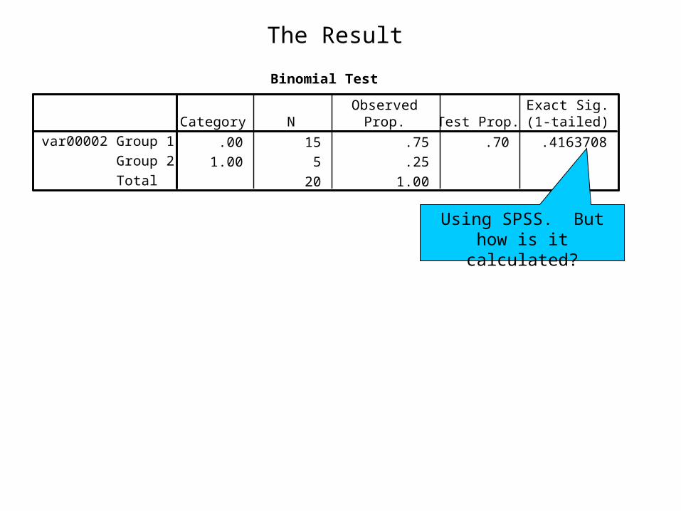
The Result

Binomial Test

.00 15 .75 .70 .4163708

1.00 5 .25

20 1.00

Group 1

Group 2

Total

var00002Category N

ObservedProp. Test Prop.

Exact Sig.(1-tailed)

Using SPSS. But how is it calculated?

How To Calculate the P-value

x P(x)0 0.000000 1 0.000000 2 0.000000 3 0.000001 4 0.000005 5 0.000037 6 0.000218 7 0.001018 8 0.003859 9 0.012007

10 0.030817 11 0.065370 12 0.114397 13 0.164262 14 0.191639 15 0.178863 16 0.130421 17 0.071604 18 0.027846 19 0.006839 20 0.000798

0

1

: .70

: .70

H p

H p

Binomial Table Made

in Excel with n=20 and p=0.70

P-value equals the sum of the probabilities 15 through 20 = .4163708

Why? P-value is the probability of observing what was observed or

more extreme under the null hypothesis. In our

example X=15 so p-value equals

P(x>=15)=.4163708

Binomial Test

Binomial Test

.00 15 .75 .70 .4163708

1.00 5 .25

20 1.00

Group 1

Group 2

Total

var00002Category N

ObservedProp. Test Prop.

Exact Sig.(1-tailed)

x=15

The way the data is analyzed it treats the “0” as a success.

There are 15 zeros.

Thus again, P-value equals the sum of the probabilities 15 through 20 =P(X>=15)= .4163708

Sampling

1. Last week we covered the Binomial distribution and Poisson distribution. 1. Count data often comes from the Binomial/Multinomial or Poisson

distribution.

2. Luckily whether the data comes from Binomial/Multinomial or Poisson distribution for most analysis of the categorical data is performed in the same manor.1. For this reason we will often not discuss which distribution the data came

from.

Two-Way Contingency Tables

Yes No/Not sure Total

Females 435 147 582

Male 375 134 509

Total 810 281 1091

Belief in AfterlifeG

ende

r

n11 n12 n1+

n21 n22 n2+

n+1 n+2 n

nrc (n, 1st row, 2nd column)

Joint, Marginal and Conditional Probabilities

sure.not areor believet don' .253 and afterlife,an is therebelieve

women of proportion .747or 147/582) (453/582, female isgender given that afterlife

in beliefon distributi lconditiona sample the,last table the Using:exampleFor

useful. very becan X|Y ofon distributi lconditiona

than theble y variaexplanatoran and varibleresponse a is If

on.distributi lconditiona theable,other vari theof leveleach given variableonefor

on distributiy probabilit separate aconstruct toeinformativ isit Often

ondistributijoint sample therepresents

:alscolumn tot and row theare onsdistributi marginal The

1 and Y and X of

on distributijoint theform tiesprobablili The

column and row cell in the falls

Y)(X,y probabilit thedenote ),(

,

,

XY

n

npnn

ji

jYiXP

ijij

jiij

iijj

jiji

jiij

ij

ij

Independence

.,...,1 and ,...,1 allfor JjIijiij

: trueholds following theceindependen lstatistica is re When theafterlife.an in believing

females ofy probabilit the toequal wasafterlifein believing males a ofy probabilit theifgender of

tindependen considered be wouldafterlifein Belief example,For X. of leveleach at identical are Y

of onsdistributi lconditiona theift independenlly statistica be tosaid are variablesTwo

Difference of Proportions

2

22

1

1121

)1()1()(ˆ

n

pp

n

pppp

96.1,05. CI, %95

)(ˆ)(

is for interval confidence The

2

212

21

21

z

ppzpp

π

When the counts in the two rows are independent binomial samples, the estimated standard error of p1-p2 is

Class take 10 minutes to do the following:

Calculate the 95% confidence interval for the difference in proportions between women and men (women-men) that believe in an afterlife.

Difference of Proportions

21 π

Now that we have calculated a 95% CI, Explain what a 95% CI is. Were we to take an infinite number of samples and create an infinite number of 95% confidence intervals 95% of those intervals created would contain the true difference of

95% CI for the difference in proportion

(can range from -1 to 1)

.010684+/-1.96*.02656

.010684+/-.052057

(-0.04137,0.062741)

Do you believe the difference is different from zero?

Difference of Proportions

Yes No Total

Placebo 189 10,845 11,034

Aspirin 104 10,933 11,037

Total 293 21,778 22,071

Myocardial Infarction (MI)G

roup

Class take 5 minutes to do the following:

Calculate a 95% for difference in proportions.

Difference in Proportions vs. Relative Risk

22

2

11

1

22

1 11log

pn

p

pn

pz

p

p

The 95% CI is (.0171-.0094)+/-1.96(0.0015)

Approx (.005,.011), appears to diminish risk of MI

Another way to compare the placebo vs. Aspirin is to look at the relative risk,

The sample relative risk is p1/p2=.0171/.0094=1.82

Thus in the sample there were 82% more cases of MI from the placebo than Aspirin. To calculate the CI for relative risk you would first calculate the CI of the log of relative risk and then take the CI limits and the taken the antilog. (Note, log will represent natural log, in Excel you must use ln, not log).

2

1

Relative Risk

The confidence interval for the relative risk is

(1.43, 2.31). From this we would the relative risk is at least 43% higher for patients taking aspirin. It can be misleading to only look at the difference in proportions, looking at this situation in terms of relative risk, clearly you would want to take Aspirin.

22

2

11

1

22

1 11log

pn

p

pn

pz

p

p

0.597628+/-1.96*0.121347=(.359787,.835469)

Exp(0.359787) and Exp(0.835469)=(1.43,2.31)

The Odds Ratio

The odds are nonnegative, when the odds are greater than one a success is more likely than a failure.

The odds ratio can equal all nonnegative numbers. When X and Y are independent then the odds ratio equals 1. An odds ratio of 4 means that the odds of success in row 1 are 4 times the odds of success in row 2. When the odds of success are higher for row 2 than row 1 the odds ratio is less than 1.

ratio. odds thecalled is This

)1(

)1(

2

1

1

2 row of odds )1(

1 row of odds )1(

2

2

1

1

2

22

1

11

odds

odds

odds

odds

odds

odds

The Odds Ratio

2112

2211

22

21

12

11

2

2

1

1n

n

)1(

)1(ˆnn

nn

nn

pp

pp

22211211

1111)ˆlog(

nnnnASE

The maximum likelihood estimator of the odds ratio is:

The asymptotic standard error for the log of the MLE is:

ˆlogˆlog

2ASEz

The confidence interval is:

Inference for Log Odds Ratios

Class take10 minutes to do the following:

Calculate the Odds ratio for MI, and then a 95% CI for the odds ratio.

Inference for Log Odds Ratios

Odds ratio=(189*10933)/(104*10845)=1.832

Log(1.832)=.605

ASE of the log = (1/189+1/10933+1/10845+1/104)1/2=.123

95% CI of the log odds ratio is (.365,.846)

Thus the 95% CI of the Odds ratio is (1.44,2.33)

Dealing with small cell counts and the

)1(

)1(Risk Relative

)1(

)1(ratioOdds

1

2

2

2

1

1

p

p

pp

pp

For when zero cell counts occur or some cell counts are very small, the following slightly amended formula is used:

)5.0)(5.0(

)5.0)(5.0(~

2112

2211

nn

nn

The Relationship Between Odds Ratio and Relative Risk

Chi-Squared Tests

ijFor calculating chi-square statistics for testing a null hypothesis with fixed values we use expected frequencies:

)1()1(

log2G

:simplifies tablescontigencyway -two

for statistic squared-chi ratio -likelihood the

log2 equals statistic test The

edunrestrict are parameters when likelihood maximum

hypothesis null under the likelihood maximum

statistic squared-chiPearson

2

2

2

JIdf

nn

nX

n

ij

ijij

ij

ijij

ijij

Chi-Squared Tests of Independence

jiijOH :

For calculating chi-square statistics for testing a null hypothesis with assuming independence:

ij

ijij

ij

ijij

jijiij

nn

nX

n

nnpnp

ˆlog2G

ˆ

ˆ

:lyrespective statistic ratio likelihood and statistic squared-chiPearson

ˆ

2

2

2

Most likely the true probabilities are unknown and the sample probabilities must be used

Chi-Squared Test of Independence

Take 15 minutes and calculate the Pearson statistic and the likelihood ratio chi-squared statistic for the null hypothesis that the probability of heads is the same for all people, assuming the true probability is unknown.

Heads Tails Total

Michael 270 230 500

Mark 260 240 500

Mary 280 220 500

Total 810 690 1500

Coin Toss

Per

son

Adjusted Residuals

jiij

ijij

pp

n

11ˆ

ˆ

When the null hypothesis is true, each adjusted residual has a large-sample standard normal distribution. An adjusted residual about 2-3 or larger in value indicates lack of fit of the null hypothesis within that cell. Take 10 minutes to calculate the adjusted residuals:

Democrat Independent Republican

Females 279 73 225

Males 165 47 191

Political Party Identification

Gen

der

Adjusted Residuals

Democrat Independent Republican

Females 279

(2.29)

73

(0.46)

225

(-2.62)

Males 165

(-2.29)

47

(-0.46)

191

(2.62)

Political Party Identification

Gen

der

From this example we can see how the adjusted residuals can add further insight beyond the chi-squared tests of independence. Such as direction.

Chi-Squared Tests of Independence with Ordinal Data

2M

,

22

2 2

1 2 3

1 2 3

2 2

scores for the rows ...

scores for the columns ...

1

1

i i j ji ji j iji j

j ji i jii i j ji j

i

i

n nn nr

nnn n

n n

M n r

df

Linear trend alternative to independence.

is chi-squared with one degree of freedom. M, its square root follows a standard normal distribution. M gives insight into direction. Note, when categories do not have scores such as education level logical scores must be assigned. E.G. High School degree =1, College degree =2, Masters degree=3

Example with Ordinal Data Alcohol and Infant Malformation

Absent Present Percentage Present

0 17,066 48 0.28

<1 14,464 38 0.26

1-2 788 5 0.63

3-5 126 1 0.79

>=6 37 1 2.63

Infant Malformation

Alc

ohol

C

onsu

mpt

ion

Take 2-3 minutes and think of logical value assignments for scores. Note: nominal binary data can be treated as ordinal.

Example with Ordinal Data Alcohol and Infant Malformation

Absent Present Percentage Present

0 17,066 48 0.28

<1 14,464 38 0.26

1-2 788 5 0.63

3-5 126 1 0.79

>=6 37 1 2.63

Infant Malformation

Alc

ohol

C

onsu

mpt

ion

1 2 3 4 5

1 2

0 0.5 1.5 4 7

0 1

Take 20 minutes using the scores given calculate r.