arxiv:quant-ph/0010034v1 9 oct 2000

arX

iv:q

uant

-ph/

0010

034v

1 9

Oct

200

0

A

LECTURE

ON

SHOR’S QUANTUM FACTORING ALGORITHM

VERSION 1.1

SAMUEL J. LOMONACO, JR.

Abstract. This paper is a written version of a one hour lecture givenon Peter Shor’s quantum factoring algorithm. It is based on [4], [6], [7],[9], and [15] .

Contents

1. Preamble to Shor’s algorithm 12. Number theoretic preliminaries 23. Overview of Shor’s algorithm 34. Preparations for the quantum part of Shor’s algorithm 55. The quantum part of Shor’s algorithm 66. Peter Shor’s stochastic source S 87. A momentary digression: Continued fractions 108. Preparation for the final part of Shor’s algorithm 119. The final part of Shor’s algorithm 1610. An example of Shor’s algorithm 17

References 21

1. Preamble to Shor’s algorithm

Date: September 20, 2000.2000 Mathematics Subject Classification. Primary: 81-01, 81P68.Key words and phrases. Shor’s algorithm, factoring, quantum computation, quantum

algorithms.This work was partially supported by ARO Grant #P-38804-PH-QC and the L-O-O-P

Fund. The author gratefully acknowledges the hospitality of the University of CambridgeIsaac Newton Institute for Mathematical Sciences, Cambridge, England, where some ofthis work was completed. I would also like to thank the other AMS Short Courselecturers, Howard Brandt, Dan Gottesman, Lou Kauffman, Alexei Kitaev, Peter Shor,Umesh Vazirani and the many Short Course participants for their support. (Copyright2000.)

1

http://arXiv.org/abs/quant-ph/0010034v1

2 SAMUEL J. LOMONACO, JR.

There are cryptographic systems (such as RSA1) that are extensivelyused today (e.g., in the banking industry) which are based on the followingquestionable assumption, i.e., conjecture:

Conjecture(Assumption). Integer factoring is computationally much

harder than integer multiplication. In other words, while there are obviously

many polynomial time algorithms for integer multiplication, there are no

polynomial time algorithms for integer factoring. I.e., integer factoring

computationally requires super-polynomial time.

This assumption is based on the fact that, in spite of the intensive effortsover many centuries of the best minds to find a polynomial time factoringalgorithm, no one has succeeded so far. As of this writing, the most asymp-totically efficient classical algorithm is the number theoretic sieve [10], [11],

which factors an integer N in time O(exp

[(lgN)1/3 (lg lgN)2/3

]). Thus,

this is a super-polynomial time algorithm in the number O (lgN) of digitsin N .

However, ... Peter Shor suddenly changed the rules of the game.

Hidden in the above conjecture is the unstated, but implicitly understood,assumption that all algorithms run on computers based on the principles ofclassical mechanics, i.e., on classical computers. But what if a computercould be built that is based not only on classical mechanics, but on quantummechanics as well? I.e., what if we could build a quantum computer?

Shor, starting from the works of Benioff, Bennett, Deutsch , Feynman,Simon, and others, created an algorithm to be run on a quantum com-puter, i.e., a quantum algorithm, that factors integers in polynomial time!

Shor’s algorithm takes asymptotically O((lgN)2 (lg lgN) (lg lg lgN)

)steps

on a quantum computer, which is polynomial time in the number of digitsO (lgN) of N .

2. Number theoretic preliminaries

Since the time of Euclid, it has been known that every positive integer Ncan be uniquely (up to order) factored into the product of primes. Moreover,

1RSA is a public key cryptographic system invented by Rivest, Shamir, Adleman.Hence the name. For more information, please refer to [17].

A LECTURE ON SHOR’S FACTORING ALGORITHM 3

it is a computationally easy (polynomial time) task to determine whether ornot N is a prime or composite number. For the primality testing algorithmof Miller-Rabin[14] makes such a determination at the cost of O (s lgN)arithmetic operations [O

(s lg3N

)bit operations] with probability of error

ProbError ≤ 2−s.

However, once an odd positive integer N is known to be composite, it doesnot appear to be an easy (polynomial time) task on a classical computer todetermine its prime factors. As mentioned earlier, so far the most asymptot-ically efficient classical algorithm known is the number theoretic sieve [10],

[11], which factors an integer N in time O(exp

[(lgN)1/3 (lg lgN)2/3

]).

Prime Factorization Problem. Given a composite odd positive integer

N , find its prime factors.

It is well known[14] that factoringN can be reduced to the task of choosingat random an integer m relatively prime to N , and then determining itsmoduloN multiplicative order P , i.e., to finding the smallest positive integerP such that

mP = 1modN .

It was precisely this approach to factoring that enabled Shor to constructhis factoring algorithm.

3. Overview of Shor’s algorithm

But what is Shor’s quantum factoring algorithm?

Let N = 0, 1, 2, 3, . . . denote the set of natural numbers.

Shor’s algorithm provides a solution to the above problem. His algorithmconsists of the five steps (steps 1 through 5), with only STEP 2 requiringthe use of a quantum computer. The remaining four other steps of thealgorithm are to be performed on a classical computer.

We begin by briefly describing all five steps. After that, we will thenfocus in on the quantum part of the algorithm, i.e., STEP 2.


Step 1. Choose a random positive integer m. Use the polynomial time Eu-

clidean algorithm2 to compute the greatest common divisor gcd (m,N)of m and N . If the greatest common divisor gcd (m,N) 6= 1, then wehave found a non-trivial factor of N , and we are done. If, on the otherhand, gcd (m,N) = 1, then proceed to STEP 2.

STEP 2. Use a quantum computer to determine the unknown period P ofthe function

NfN−→ N

a 7−→ ma modN

Step 3. If P is an odd integer, then goto Step 1. [The probability of P being

odd is (12)k, where k is the number of distinct prime factors of N .] If

P is even, then proceed to Step 4.

Step 4. Since P is even,(mP/2 − 1

) (mP/2 + 1

)= mP − 1 = 0modN .

If mP/2 + 1 = 0modN , then goto Step 1. If mP/2 + 1 6= 0modN ,then proceed to Step 5. It can be shown that the probability thatmP/2 + 1 = 0modN is less than (1

2)k−1, where k denotes the numberof distinct prime factors of N .

Step 5. Use the Euclidean algorithm to compute d = gcd(mP/2 − 1, N

). Since

mP/2+1 6= 0modN , it can easily be shown that d is a non-trivial factorof N . Exit with the answer d.

Thus, the task of factoring an odd positive integer N reduces to thefollowing problem:

Problem. Given a periodic function

f : N −→ N ,

find the period P of f .

2The Euclidean algorithm is O(lg2 N

). For a description of the Euclidean algorithm,

see for example [3] or [2].


4. Preparations for the quantum part of Shor’s algorithm

Choose a power of 2

Q = 2L

such that

N2 ≤ Q = 2L < 2N2 ,

and consider f restricted to the set

SQ = 0, 1, . . . , Q− 1which we also denote by f , i.e.,

f : SQ −→ SQ .

In preparation for a discussion of STEP 2 of Shor’s algorithm, we con-struct two L-qubit quantum registers, Register1 and Register2 to holdrespectively the arguments and the values of the function f , i.e.,

|Reg1〉 |Reg2〉 = |a〉 |f(a)〉 = |a〉 |b〉 = |a0a1 · · · aL−1〉 |b0b1 · · · bL−1〉In doing so, we have adopted the following convention for representing

integers in these registers:

Notation Convention. In a quantum computer, we represent an integer

a with radix 2 representation

a =

L−1∑

j=0

aj2j ,

as a quantum register consisting of the 2n qubits

|a〉 = |a0a1 · · · aL−1〉 =L−1⊗

j=0

|aj〉

For example, the integer 23 is represented in our quantum computer as nqubits in the state:

|23〉 = |10111000 · · · 0〉

Before continuing, we remind the reader of the classical definition of theQ-point Fourier transform.


Definition 1. Let ω be a primitive Q-th root of unity, e.g., ω = e2πi/Q.

Then the Q-point Fourier transform is the map

Map(SQ,C)F−→Map(SQ,C)

[f : SQ −→ C] 7−→[f : SQ −→ C

]

where

f (y) =1√Q

∑

x∈SQ

f(x)ωxy

We implement the Fourier transform F as a unitary transformation, whichin the standard basis

|0〉 , |1〉 , . . . , |Q− 1〉is given by the Q×Q unitary matrix

F =1√Q

(ωxy) .

This unitary transformation can be factored into the product of O(lg2Q

)=

O(lg2N

)sufficiently local unitary transformations. (See [15], [6].)

5. The quantum part of Shor’s algorithm

The quantum part of Shor’s algorithm, i.e., STEP 2, is the following:

STEP 2.0 Initialize registers 1 and 2, i.e.,

|ψ0〉 = |Reg1〉 |Reg2〉 = |0〉 |0〉 = |00 · · · 0〉 |0 · · · 0〉STEP 2.1 3Apply the Q-point Fourier transform F to Register1.

|ψ0〉 = |0〉 |0〉 F⊗I7−→ |ψ1〉 =1√Q

Q−1∑

x=0

ω0·x |x〉 |0〉 =1√Q

Q−1∑

x=0

|x〉 |0〉

Remark 1. Hence, Register1 now holds all the integers

0, 1, 2, . . . , Q− 1

in superposition.

3In this step we could have instead applied the Hadamard transform to Register1

with the same result, but at the computational cost of O (lg N) sufficiently local unitarytransformations. The term sufficiently local unitary transformationis defined in the lastpart of section 7.7 of [13].


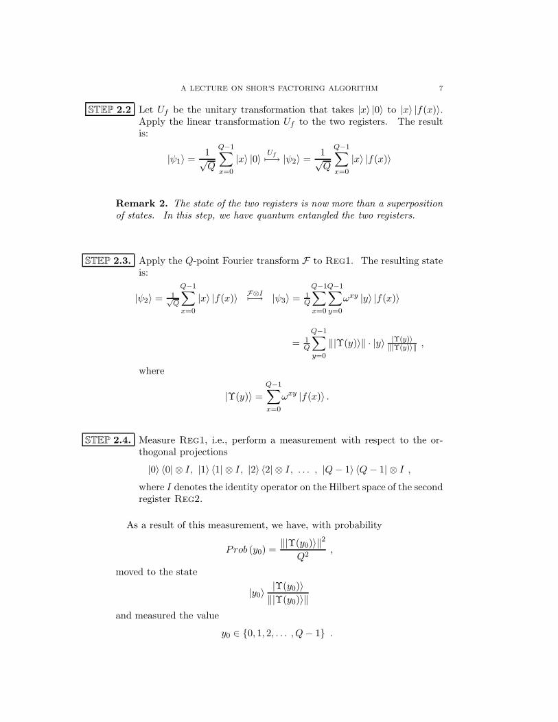
STEP 2.2 Let Uf be the unitary transformation that takes |x〉 |0〉 to |x〉 |f(x)〉.Apply the linear transformation Uf to the two registers. The resultis:

|ψ1〉 =1√Q

Q−1∑

x=0

|x〉 |0〉 Uf7−→ |ψ2〉 =1√Q

Q−1∑

x=0

|x〉 |f(x)〉

Remark 2. The state of the two registers is now more than a superposition

of states. In this step, we have quantum entangled the two registers.

STEP 2.3. Apply the Q-point Fourier transform F to Reg1. The resulting stateis:

|ψ2〉 = 1√Q

Q−1∑

x=0

|x〉 |f(x)〉 F⊗I7−→ |ψ3〉 = 1Q

Q−1∑

x=0

Q−1∑

y=0

ωxy |y〉 |f(x)〉

= 1Q

Q−1∑

y=0

‖|Υ(y)〉‖ · |y〉 |Υ(y)〉‖|Υ(y)〉‖ ,

where

|Υ(y)〉 =Q−1∑

x=0

ωxy |f(x)〉 .

STEP 2.4. Measure Reg1, i.e., perform a measurement with respect to the or-thogonal projections

|0〉〈0| ⊗ I, |1〉〈1| ⊗ I, |2〉〈2| ⊗ I, . . . , |Q− 1〉〈Q− 1| ⊗ I ,

where I denotes the identity operator on the Hilbert space of the secondregister Reg2.

As a result of this measurement, we have, with probability

Prob (y0) =‖|Υ(y0)〉‖2

Q2,

moved to the state

|y0〉|Υ(y0)〉‖|Υ(y0)〉‖

and measured the value

y0 ∈ 0, 1, 2, . . . , Q− 1 .


If after this computation, we ignore the two registers Reg1 and Reg2, wesee that what we have created is nothing more than a classical probabilitydistribution S on the sample space

0, 1, 2, . . . , Q− 1 .

In other words, the sole purpose of executing STEPS 2.1 to 2.4 is to createa classical finite memoryless stochastic source S which outputs a symboly0 ∈ 0, 1, 2, . . . , Q− 1 with the probability

Prob(y0) =‖|Υ(y0)〉‖2

Q2.

(For more details, please refer to section 8.1 of [13].)

As we shall see, the objective of the remander of Shor’s algorithm is toglean information about the period P of f from the just created stochasticsource S. The stochastic source was created exactly for that reason.

6. Peter Shor’s stochastic source S

Before continuing to the final part of Shor’s algorithm, we need to analyzethe probability distribution Prob (y) a little more carefully.

Proposition 1. Let q and r be the unique non-negative integers such that

Q = Pq + r , where 0 ≤ r < P ; and let Q0 = Pq. Then

Prob (y) =

r sin2(

πPy

Q·(

Q0P

+1))

+(P−r) sin2(

πPy

Q·Q0

P

)

Q2 sin2(

πPy

Q

) if Py 6= 0modQ

r(Q0+P )2+(P−r)Q20

Q2P 2 if Py = 0modQ


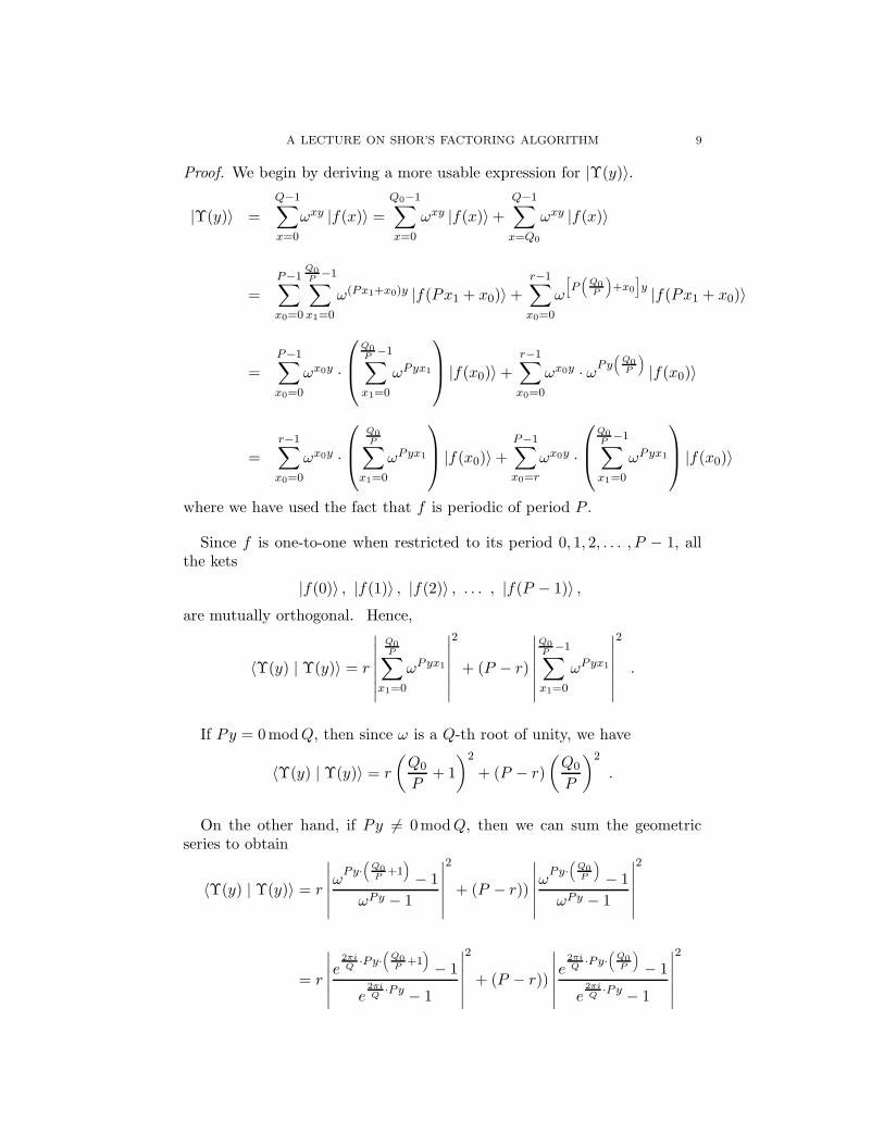
Proof. We begin by deriving a more usable expression for |Υ(y)〉.

|Υ(y)〉 =

Q−1∑

x=0

ωxy |f(x)〉 =Q0−1∑

x=0

ωxy |f(x)〉+Q−1∑

x=Q0

ωxy |f(x)〉

=

P−1∑

x0=0

Q0P

−1∑

x1=0

ω(Px1+x0)y |f(Px1 + x0)〉+r−1∑

x0=0

ω

[P

(Q0P

)+x0

]y |f(Px1 + x0)〉

=

P−1∑

x0=0

ωx0y ·

Q0P

−1∑

x1=0

ωPyx1

|f(x0)〉+r−1∑

x0=0

ωx0y · ωPy(

Q0P

)

|f(x0)〉

=

r−1∑

x0=0

ωx0y ·

Q0P∑

x1=0

ωPyx1

|f(x0)〉+P−1∑

x0=r

ωx0y ·

Q0P

−1∑

x1=0

ωPyx1

|f(x0)〉

where we have used the fact that f is periodic of period P .

Since f is one-to-one when restricted to its period 0, 1, 2, . . . , P − 1, allthe kets

|f(0)〉 , |f(1)〉 , |f(2)〉 , . . . , |f(P − 1)〉 ,are mutually orthogonal. Hence,

〈Υ(y) | Υ(y)〉 = r

∣∣∣∣∣∣∣

Q0P∑

x1=0

ωPyx1

∣∣∣∣∣∣∣

2

+ (P − r)

∣∣∣∣∣∣∣

Q0P

−1∑

x1=0

ωPyx1

∣∣∣∣∣∣∣

2

.

If Py = 0modQ, then since ω is a Q-th root of unity, we have

〈Υ(y) | Υ(y)〉 = r

(Q0

P+ 1

)2

+ (P − r)(Q0

P

)2

.

On the other hand, if Py 6= 0modQ, then we can sum the geometricseries to obtain

〈Υ(y) | Υ(y)〉 = r

∣∣∣∣∣∣ω

Py·(

Q0P

+1)

− 1

ωPy − 1

∣∣∣∣∣∣

2

+ (P − r))

∣∣∣∣∣∣ω

Py·(

Q0P

)

− 1

ωPy − 1

∣∣∣∣∣∣

2

= r

∣∣∣∣∣∣e

2πiQ

·Py·(

Q0P

+1)

− 1

e2πiQ

·Py − 1

∣∣∣∣∣∣

2

+ (P − r))

∣∣∣∣∣∣e

2πiQ

·Py·(

Q0P

)

− 1

e2πiQ

·Py − 1

∣∣∣∣∣∣

2


where we have used the fact that ω is the primitive Q-th root of unity givenby

ω = e2πi/Q .

The remaining part of the proposition is a consequence of the trigono-metric identity

∣∣∣eiθ − 1∣∣∣2

= 4 sin2

(θ

2

).

As a corollary, we have

Corollary 1. If P is an exact divisor of Q, then

Prob (y) =

0 if Py 6= 0modQ

1P if Py = 0modQ

7. A momentary digression: Continued fractions

We digress for a moment to review the theory of continued fractions. (Fora more in-depth explanation of the theory of continued fractions, please referto [5] and [12].)

Every positive rational number ξ can be written as an expression in theform

ξ = a0 +1

a1 +1

a2+1

a3+

1

···+1

aN

,

where a0 is a non-negative integer, and where a1, . . . , aN are positive inte-gers. Such an expression is called a (finite, simple) continued fraction,and is uniquely determined by ξ provided we impose the condition aN > 1.For typographical simplicity, we denote the above continued fraction by

[a0, a1, . . . , aN ] .


The continued fraction expansion of ξ can be computed with the followingrecurrence relation, which always terminates if ξ is rational:

a0 = ⌊ξ⌋

ξ0 = ξ − a0

, and if ξn 6= 0, then

an+1 = ⌊1/ξn⌋

ξn+1 = 1ξn− an+1

The n-th convergent (0 ≤ n ≤ N) of the above continued fraction isdefined as the rational number ξn given by

ξn = [a0, a1, . . . , an] .

Each convergent ξn can be written in the form, ξn = pn

qn, where pn and qn

are relatively prime integers ( gcd (pn, qn) = 1). The integers pn and qn aredetermined by the recurrence relation

p0 = a0, p1 = a1a0 + 1, pn = anpn−1 + pn−2,

q0 = 1, q1 = a1, qn = anqn−1 + qn−2 .

8. Preparation for the final part of Shor’s algorithm

Definition 2. 4For each integer a, let aQ denote the residue of a

modulo Q of smallest magnitude. In other words, aQ is the unique

integer such that

a = aQ modQ

−Q/2 < aQ ≤ Q/2.

Proposition 2. Let y be an integer lying in SQ. Then

Prob (y) ≥

4π2 · 1

P ·(1− 1

N

)2if 0 <

∣∣∣PyQ∣∣∣ ≤ P

2 ·(1− 1

N

)

1P ·

(1− 1

N

)2if PyQ = 0

4aQ

= a − Q · round(

aQ

)= a − Q ·

⌊aQ

+ 1

2

⌋.


Proof. We begin by noting that∣∣∣πPyQ

Q ·(

Q0

P + 1)∣∣∣ ≤ π

Q · P2 ·

(1− 1

N

)·(

Q0+PP

)≤ π

2 ·(1− 1

N

)·(

Q+PQ

)

≤ π2 ·

(1− 1

N

)·(1 + P

Q

)≤ π

2 ·(1− 1

N

)·(1 + N

N2

)< π

2 ,

where we have made use of the inequalities

N2 ≤ Q < 2N2 and 0 < P ≤ N .

It immediately follows that∣∣∣∣π PyQ

Q· Q0

P

∣∣∣∣ <π

2.

As a result, we can legitimately use the inequality

4π2θ2 ≤ sin2 θ ≤ θ2, for |θ| < π

2

to simplify the expression for Prob (y).

Thus,

Prob (y) =r sin2

(πPyQ

Q·(

Q0P

+1))

+(P−r) sin2

(πPyQ

Q·Q0

P

)

Q2 sin2(

πPy

Q

)

≥r· 4

π2 ·(

πPyQ

Q·(

Q0P

+1))2

+(P−r)· 4

π2 ·(

πPyQ

Q·Q0

P

)2

Q2

(πPyQ

Q

)2

≥ 4π2 ·

P ·(

Q0P

)2

Q2 = 4π2 · 1

P ·(

Q−rQ

)2

= 4π2 · 1

P ·(1− r

Q

)2≥ 4

π2 · 1P ·

(1− 1

N

)2

The remaining case, PyQ = 0 is left to the reader.

Lemma 1. Let

Y =

y ∈ SQ |

∣∣∣PyQ∣∣∣ ≤ P

2

and SP = d ∈ SQ | 0 ≤ d < P .

Then the map

Y −→ SP

y 7−→ d = d(y) = round(

PQ · y

)


is a bijection with inverse

y = y(d) = round

(Q

P· d

).

Hence, Y and SP are in one-to-one correspondence. Moreover,

PyQ = P · y −Q · d(y) .

Remark 3. Moreover, the following two sets of rationals are in one-to-one

correspondencey

Q| y ∈ Y

←→

d

P| 0 ≤ d < P

As a result of the measurement performed in STEP 2.4, we have in ourpossession an integer y ∈ Y . We now show how y can be use to determinethe unknown period P .

We now need the following theorem5 from the theory of continued frac-tions:

Theorem 1. Let ξ be a real number, and let a and b be integers with b > 0.If

∣∣∣ξ − a

b

∣∣∣ ≤ 1

2b2,

then the rational number a/b is a convergent of the continued fraction ex-

pansion of ξ.

As a corollary, we have:

Corollary 2. If

∣∣∣PyQ∣∣∣ ≤ P

2 , then the rational numberd(y)P is a convergent

of the continued fraction expansion of yQ .

Proof. Since

Py −Qd(y) = PyQ ,

we know that

|Py −Qd(y)| ≤ P

2,

which can be rewritten as ∣∣∣∣y

Q− d(y)

P

∣∣∣∣ ≤1

2Q.

5See [5, Theorem 184, Section 10.15].


But, since Q ≥ N2, it follows that∣∣∣∣y

Q− d(y)

P

∣∣∣∣ ≤1

2N2.

Finally, since P ≤ N (and hence 12N2 ≤ 1

2P 2 ), the above theorem can be

applied. Thus, d(y)P is a convergent of the continued fraction expansion of

ξ = yQ .

Since d(y)P is a convergent of the continued fraction expansion of y

Q , it

follows that, for some n,

d(y)

P=pn

qn,

where pn and qn are relatively prime positive integers given by a recurrencerelation found in the previous subsection. So it would seem that we havefound a way of deducing the period P from the output y of STEP 2.4, andso we are done.

Not quite!

We can determine P from the measured y produced by STEP 2.4, only if

pn = d(y)

qn = P,

which is true only when d(y) and P are relatively prime.

So what is the probability that the y ∈ Y produced by STEP 2.4 satisfiesthe additional condition that

gcd (P, d(y)) = 1 ?

Proposition 3. The probability that the random y produced by STEP 2.4 is

such that d(y) and P are relatively prime is bounded below by the following

expression

Prob y ∈ Y | gcd(d(y), P ) = 1 ≥ 4

π2· φ(P )

P·(

1− 1

N

)2

,

where φ(P ) denotes Euler’s totient function, i.e., φ(P ) is the number of

positive integers less than P which are relatively prime to P .

The following theorem can be found in [5, Theorem 328, Section 18.4]:


Theorem 2.

lim infφ(N)

N/ ln lnN= e−γ,

where γ denotes Euler’s constant γ = 0.57721566490153286061 . . . , and

where e−γ = 0.5614594836 . . . .

As a corollary, we have:

Corollary 3.

Prob y ∈ Y | gcd(d(y), P ) = 1 ≥ 4

π2 ln 2· e

−γ − ǫ (P )

lg lgN·(

1− 1

N

)2

,

where ǫ (P ) is a monotone decreasing sequence converging to zero. In terms

of asymptotic notation,

Prob y ∈ Y | gcd(d(y), P ) = 1 = Ω

(1

lg lgN

).

Thus, if STEP 2.4 is repeated O(lg lgN) times, then the probability of suc-

cess is Ω (1).

Proof. From the above theorem, we know that

φ(P )

P/ ln lnP≥ e−γ − ǫ (P ) .

where ǫ (P ) is a monotone decreasing sequence of positive reals convergingto zero. Thus,

φ(P )

P≥ e−γ − ǫ (P )

ln lnP≥ e−γ − ǫ (P )

ln lnN=

e−γ − ǫ (P )

ln ln 2 + ln lgN≥ e−γ − ǫ (P )

ln 2· 1

lg lgN

Remark 4. Ω( 1lg lg N ) denotes an asymptotic lower bound. Readers not

familiar with the big-oh O(∗) and big-omega Ω (∗) notation should refer to

[2, Chapter 2] or [1, Chapter 2].


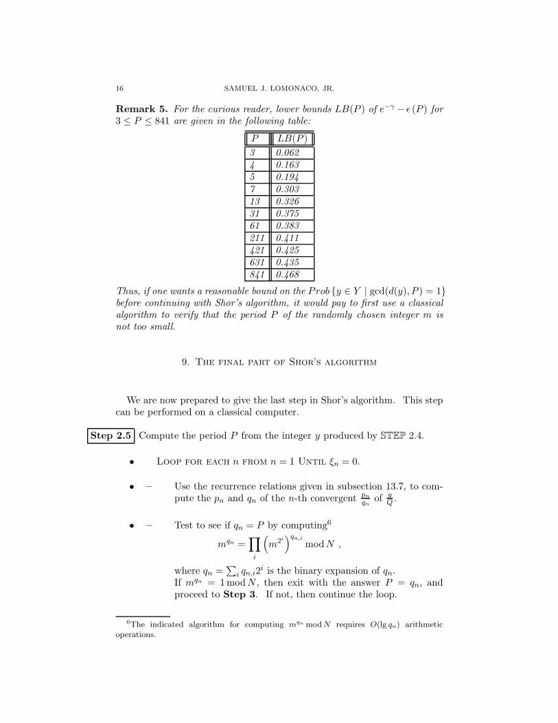
Remark 5. For the curious reader, lower bounds LB(P ) of e−γ − ǫ (P ) for

3 ≤ P ≤ 841 are given in the following table:

P LB(P )

3 0.062

4 0.163

5 0.194

7 0.303

13 0.326

31 0.375

61 0.383

211 0.411

421 0.425

631 0.435

841 0.468

Thus, if one wants a reasonable bound on the Prob y ∈ Y | gcd(d(y), P ) = 1before continuing with Shor’s algorithm, it would pay to first use a classical

algorithm to verify that the period P of the randomly chosen integer m is

not too small.

9. The final part of Shor’s algorithm

We are now prepared to give the last step in Shor’s algorithm. This stepcan be performed on a classical computer.

Step 2.5 Compute the period P from the integer y produced by STEP 2.4.

• Loop for each n from n = 1 Until ξn = 0.

• – Use the recurrence relations given in subsection 13.7, to com-pute the pn and qn of the n-th convergent pn

qnof y

Q .

• – Test to see if qn = P by computing6

mqn =∏

i

(m2i

)qn,i

modN ,

where qn =∑

i qn,i2i is the binary expansion of qn.

If mqn = 1modN , then exit with the answer P = qn, andproceed to Step 3. If not, then continue the loop.

6The indicated algorithm for computing mqn mod N requires O(lg qn) arithmeticoperations.


• End of Loop

• If you happen to reach this point, you are a very unlucky quantumcomputer scientist. You must start over by returning to STEP

2.0. But don’t give up hope! The probability that the integer yproduced by STEP 2.4 will lead to a successful completion of Step2.5 is bounded below by

4

π2 ln 2· e

−γ − ǫ (P )

lg lgN·(

1− 1

N

)2

>0.232

lg lgN·(

1− 1

N

)2

,

provided the period P is greater than 3. [ γ denotes Euler’sconstant.]

10. An example of Shor’s algorithm

Let us now show how N = 91 (= 7 · 13) can be factored using Shor’salgorithm.

We choose Q = 214 = 16384 so that N2 ≤ Q < 2N2.

Step 1 Choose a random positive integer m, say m = 3. Since gcd(91, 3) = 1,

we proceed to STEP 2 to find the period of the function f given by

f(a) = 3a mod91

Remark 6. Unknown to us, f has period P = 6. For,

a 0 1 2 3 4 5 6 7 · · ·

f(a) 1 3 9 27 81 61 1 3 · · ·∴ Unknown period P = 6

STEP 2.0 Initialize registers 1 and 2. Thus, the state of the two registers becomes:

|ψ0〉 = |0〉 |0〉


STEP 2.1 Apply the Q-point Fourier transform F to register #1, where

F |k〉 = 1√16384

16383∑

x=0

ω0·x |x〉 ,

and where ω is a primitive Q-th root of unity, e.g., ω = e2πi

16384 . Thusthe state of the two registers becomes:

|ψ1〉 =1√

16384

16383∑

x=0

|x〉 |0〉

STEP 2.2 Apply the unitary transformation Uf to registers #1 and #2, where

Uf |x〉 |ℓ〉 = |x〉 | f(x)− ℓ mod 91〉 .

(Please note that U2f = I.) Thus, the state of the two registers becomes:

|ψ2〉 = 1√16384

∑16383x=0 |x〉 |3x mod91〉

= 1√16384

( | 0〉 |1〉 + | 1〉 |3〉+ | 2〉 |9〉 + | 3〉 |27〉+ | 4〉 |81〉 + | 5〉 |61〉

+ | 6〉 |1〉 + | 7〉 |3〉+ | 8〉 |9〉 + | 9〉 |27〉 + |10〉 |81〉+ |11〉 |61〉

+ |12〉 |1〉 + |13〉 |3〉 + |14〉 |9〉 + |15〉 |27〉 + |16〉 |81〉 + |17〉 |61〉

+ . . .

+ |16380〉 |1〉+ |16381〉 |3〉+ |16382〉 |9〉+ |16383〉 |27〉)

Remark 7. The state of the two registers is now more than a superposition

of states. We have in the above step quantum entangled the two registers.

STEP 2.3 Apply the Q-point F again to register #1. Thus, the state of thesystem becomes:

|ψ3〉 = 1√16384

∑16383x=0

1√16384

∑16383y=0 ωxy |y〉 |3x mod91〉

= 116384

∑16383x=0 |y〉

∑16383x=0 ωxy |3x mod91〉

= 116384

∑16383x=0 |y〉 |Υ (y)〉 ,


where

|Υ (y)〉 =

16383∑

x=0

ωxy |3x mod91〉

Thus,

|Υ (y)〉 = |1〉 + ωy |3〉+ ω2y |9〉 + ω3y |27〉 + ω4y |81〉 + ω5y |61〉

+ ω6y |1〉 + ω7y |3〉+ ω8y |9〉 + ω9y |27〉 + ω10y |81〉 + ω11y |61〉

+ ω12y |1〉 + ω13y |3〉+ ω14y |9〉 + ω15y |27〉 + ω16y |81〉+ ω17y |61〉

+ . . .

+ ω16380y |1〉+ ω16381y |3〉+ ω16382y |9〉+ ω16383y |27〉

STEP 2.4 Measure Reg1. The result of our measurement just happens to turnout to be

y = 13453

Unknown to us, the probability of obtaining this particular y is:

0.3189335551 × 10−6 .

Moreover, unknown to us, we’re lucky! The corresponding d is relativelyprime to P , i.e.,

d = d(y) = round(P

Q· y) = 5

However, we do know that the probability of d(y) being relatively primeto P is greater than

0.232

lg lgN·(

1− 1

N

)2

≈ 8.4% (provided P > 3),

and we also know that

d(y)

P

is a convergent of the continued fraction expansion of

ξ =y

Q=

13453

16384

So with a reasonable amount of confidence, we proceed to Step 2.5.


Step 2.5 Using the recurrence relations found in subsection 13.7 of this paper,

we successively compute (beginning with n = 0) the an’s and qn’s forthe continued fraction expansion of

ξ =y

Q=

13453

16384.

For each non-trivial n in succession, we check to see if

3qn = 1mod 91.

If this is the case, then we know qn = P , and we immediately exit fromStep 2.5 and proceed to Step 3.

• In this example, n = 0 and n = 1 are trivial cases.

• For n = 2, a2 = 4 and q2 = 5 . We test q2 by computing

3q2 = 35 =(320

)1·(321

)0·(320

)1= 61 6= 1mod 91 .

Hence, q2 6= P .

• We proceed to n = 3, and compute

a3 = 1 and q3 = 6.

We then test q3 by computing

3q3 = 36 =(320

)0·(321

)1·(320

)1= 1mod 91 .

Hence, q3 = P . Since we now know the period P , there is no needto continue to compute the remaining an’s and qn’s. We proceedimmediately to Step 3.

To satisfy the reader’s curiosity we have listed in the table below all thevalues of an, pn, and qn for n = 0, 1, . . . , 14. But it should be mentionedagain that we need only to compute an and qn for n = 0, 1, 2, 3, as indicatedabove.

n 0 1 2 3 4 5 6 7 8 9 10 11 12 13 14

an 0 1 4 1 1 2 3 1 1 3 1 1 1 1 3pn 0 1 4 5 9 23 78 101 179 638 817 1455 2272 3727 13453qn 1 1 5 6 11 28 95 123 218 777 995 1772 2767 4539 16384

Step 3. Since P = 6 is even, we proceed to Step 4.

Step 4. Since

3P/2 = 33 = 27 6= −1mod91,

we goto Step 5.


Step 5. With the Euclidean algorithm, we compute

gcd(3P/2 − 1, 91

)= gcd

(33 − 1, 91

)= gcd (26, 91) = 13 .

We have succeeded in finding a non-trivial factor of N = 91, namely13. We exit Shor’s algorithm, and proceed to celebrate!

References

[1] Brassard, Gilles, and Paul Bratley, “Algorithmics: Theory and Practice,”

Printice-Hall, (1988).[2] Cormen, Thomas H., Charles E. Leiserson, and Ronald L. Rivest, “Introduction to

Algorithms,” McGraw-Hill, (1990).[3] Cox, David, John Little, and Donal O’Shea, “Ideals, Varieties, and Algorithms,”

(second edition), Springer-Verlag, (1996).[4] Ekert, Artur K.and Richard Jozsa, Quantum computation and Shor’s factoring

algorithm, Rev. Mod. Phys., 68,(1996), pp 733-753.[5] Hardy, G.H., and E.M. Wright, “An Introduction to the Theory of Numbers,”

Oxford Press, (1965).[6] Hoyer, Peter, Efficient quantum transforms, quant-ph/9702028.[7] Jozsa, Richard, Quantum algorithms and the Fourier transform, quant-ph

preprint archive 9707033 17 Jul 1997.[8] Jozsa, Richard, Proc. Roy. Soc. London Soc., Ser. A, 454, (1998), 323 - 337.[9] Kitaev, A., Quantum measurement and the abelian stabiliser problem,

(1995), quant-ph preprint archive 9511026.[10] Lenstra, A.K., and H.W. Lenstra, Jr., eds., “The Development of the Number

Field Sieve,” Lecture Notes in Mathematics, Vol. 1554, Springer-Velag, (1993).[11] Lenstra, A.K., H.W. Lenstra, Jr., M.S. Manasse, and J.M. Pollard, The number

field sieve. Proc. 22nd Annual ACM Symposium on Theory of ComputingACM,New York, (1990), pp 564 - 572. (See exanded version in Lenstra & Lenstra, (1993),pp 11 - 42.)

[12] LeVeque, William Judson, “Topics in Number Theory: Volume I,” Addison-Wesley, (1958).

[13] Lomonaco, Samuel J., Jr., A Rosetta Stone for quantum mechanics with an

introduction to quantum computation: Lecture Notes for the AMS Short

Course on Quantum Computation, Washington, DC, January 2000, in“Quantum Computation,” edited by S.J. Lomonaco, Jr., AMS PSAPM Series.(to appear)

[14] Miller, G. L., Riemann’s hypothesis and tests for primality, J. Comput. SystemSci., 13, (1976), pp 300 - 317.

[15] Shor, Peter W., Polynomial time algorithms for prime factorization and

discrete logarithms on a quantum computer, SIAM J. on Computing, 26(5)(1997), pp 1484 - 1509. (quant-ph/9508027)

[16] Shor, Peter W., Introduction to quantum algorithms, Lecture Notes for the

AMS Short Course on Quantum Computation, Washington, DC, January

2000,” to appear in “Quantum Computation,” edited by S.J. Lomonaco, AMSPSAPM Series. (To appear) (quant-ph/0005003)

[17] Stinson, Douglas R., “Cryptography: Theory and Practice,” CRC Press, BocaRaton, (1995).

http://arXiv.org/abs/quant-ph/9702028




Dept. of Comp. Sci. & Elect. Engr., University of Maryland Baltimore

County, 1000 Hilltop Circle, Baltimore, MD 21250

E-mail address: E-Mail: [email protected]

URL: WebPage: http://www.csee.umbc.edu/~lomonaco

http://www.csee.umbc.edu/~lomonaco

arxiv:quant-ph/0010034v1 9 oct 2000

Documents