arX

iv:h

ep-t

h/00

0222

2v3

31

Mar

200

0

February 1, 2008 HUTP-00/A005

hep-th/0002222

Mirror Symmetry

Kentaro Hori and Cumrun Vafa

Jefferson Physical Laboratory, Harvard University

Cambridge, MA 02138, U.S.A.

Abstract

We prove mirror symmetry for supersymmetric sigma models on Kahler

manifolds in 1+1 dimensions. The proof involves establishing the equivalence

of the gauged linear sigma model, embedded in a theory with an enlarged

gauge symmetry, with a Landau-Ginzburg theory of Toda type. Standard

R → 1/R duality and dynamical generation of superpotential by vortices are

crucial in the derivation. This provides not only a proof of mirror symmetry

in the case of (local and global) Calabi-Yau manifolds, but also for sigma

models on manifolds with positive first Chern class, including deformations of

the action by holomorphic isometries.

1 Introduction

One of the most beautiful symmetries in string theory is the radius inversion symmetry

R → 1/R of a circle, known as T-duality [1]. This is the symmetry which exchanges

winding modes on a circle with momentum modes on the dual circle. This symmetry has

been the underlying motivation for many of the subsequent dualities discovered in string

theory and in quantum field theories. In particular, over a decade ago, it was conjectured

in [2, 3] that a similar duality might exist in the context of string propagation on Calabi-

Yau manifolds, where the role of the complex deformations on one manifold get exchanged

with the Kahler deformations on the dual manifold. The pairs of manifolds satisfying this

symmetry are known as mirror pairs, and this duality is also called mirror symmetry.

There has been a lot of progress since the original formulation of this conjecture, in

its support. In particular many examples of this phenomenon were found [4, 5]. The

intermediate step in the derivation for this class of examples involved the construction

of conformal field theory for certain Calabi-Yau’s [6] and their identification with certain

Landau-Ginzburg models [7–9]. This connection was further elucidated in [10] where it

was shown that the linear sigma model is a powerful tool in the study of strings propa-

gating on a Kahler manifold.

It was shown in [11] how mirror symmetry can be used very effectively to gain in-

sight into non-perturbative effects involving worldsheet instantons. Roughly speaking

this amounts to counting the number of holomorphic curves in a Calabi-Yau manifold.

This made the subject also interesting for algebraic geometers in the context of enumera-

tive geometry. Motivated by the existing examples some general class of mirror pairs were

formulated by mathematicians using toric geometry [12]. Moreover a program to prove

the rational curve counting formula, predicted by mirror symmetry, from the view point

of localization and virtual fundamental cycles was initiated in [13–15] and was pushed

to completion in [16–19]. For reviews of various aspects of mirror symmetry see [20]; for

mathematical aspects of mirror symmetry see the excellent book [21].

The question of a proof of mirror symmetry and its relation with T-duality, which was

its original motivation, was further pursued in [22] where it was shown that for certain

toroidal orbifold models mirror symmetry reduces to T-duality. More generally, by follow-

ing the prediction of the map of D-branes under mirror symmetry, it was argued in [23]

that mirror symmetry should reduce to T-duality in a more general context. Furthermore,

it was shown in [24], how the general suggestion for construction of mirror pairs proposed

using toric geometry [12] can be intuitively related to T-duality.

1

Mirror symmetry has also been extended from the case of Calabi-Yau sigma models to

more general cases. On the one hand there are proposals as to what the mirror theories

are in the case of certain sigma models with positive first Chern class [25–29, 16]. On the

other hand there are proposals for what the mirror of non-compact Calabi-Yau manifolds

are [30–32].

The aim of this paper is to present a proof of mirror symmetry for all cases proposed

thus far. The proof depends crucially on establishing a dual description of (2, 2) super-

symmetric gauge theories in 1+1 dimensions. The dual theory is found using the idea

analogous to Polyakov’s model of confinement in quantum electrodymanics in 2 + 1 di-

mensions [33]. He considered a U(1) gauge theory which includes magnetic monopoles

playing the role of instantons. U(1) Maxwell theory of gauge coupling constant e in 2+ 1

dimensions is dual to the theory of a periodic scalar field σ ≡ σ+2π with the Lagrangian

e2|dσ|2. The gas of instantons and anti-instantons with a long range interaction between

them generates a potential term

U(σ) = µ3 cos(σ) (1.1)

in the effective Lagrangian in terms of the dual variable σ, where µ is the mass scale

determined by e and the monopole size. One sees from this that a mass gap is generated

and that an electric flux is confined into a thin tube. We note that the description in

terms of the dual variable σ was essential in this argument.

In supersymmetric field theories, instanton computation can be used to obtain exact

results for some important physical quantities. For some of the striking examples, see [34–

39]. Among these, [34] and [39] treat supersymmetric gauge theories in 2 + 1 dimensions

and the effective theory is described in terms of the dual variable as in [33]. Also, in [38],

duality between vector and vector in 3 + 1 dimensions was used to solve the problem in

an essential way.

We apply an analogous idea to study the long distance behaviour of (2, 2) gauge theo-

ries, making use of instantons which are vortices [40] in this case. We dualize the phase of

the charged fields in the sense of R → 1/R duality and describe the low energy effective

theory in terms of the dual variables. We will see that a superpotential is dynamically gen-

erated by the instanton effect, as in [33–35], and we can exactly determine the (twisted)

F-term part of the effective Lagrangian. To be specific, let us consider a (2, 2) supersym-

metric U(1) gauge theory with N chiral multiplets of charge Qi (i = 1, . . . , N). In addition

to the gauge coupling, the theory has two parameters: Fayet-Iliopoulos and Theta param-

eters. They are combined into a single complex parameter t and appear in the twisted

superpotential as −tΣ where Σ is the twisted chiral field which is the field strength of

2

the gauge multiplet (and includes the scalar, the gaugino and the field strength). Each

charged chiral field is sent by the duality on its phase to a twisted chiral field Yi which is

a neutral periodic variable Yi ≡ Yi +2πi that couples to the field strength as a dynamical

Theta angle QiYiΣ. The exact twisted superpotential we will find is given by

W = Σ

(N∑

i=1

QiYi − t

)+ µ

N∑

i=1

e−Yi, (1.2)

where µ is a scale parameter. The term proportional to Σ is the one that appears already

at the dualization process. The exponentials of Yi’s are the ones that are generated by

instanton effect. When∑

iQi 6= 0, µ is a scale required to renormalize the FI parameter

t. In this case, a combination of t and µ is a fake and only one dimensionful parameter

Λ = µe−t/∑

iQi is the real parameter of the theory. This is the standard dimensional

transmutation. In the case where∑

iQi = 0, t is the dimensionless parameter of the

theory and µ is a fake as it can be absorbed by a field redefinition.

Using the connection between U(1) gauge theories with matter and sigma models

on Kahler manifolds [10] we then relate the above result to the statement of mirror

symmetry1. In particular we find that the mirror to a sigma model is a Landau-Ginzburg

model. In the case of Calabi-Yau manifolds this can also be related to the sigma model on

another Calabi-Yau manifold by the equivalence of sigma models and Landau-Ginzburg

models. In the case of manifolds with non-zero first Chern class, however, this is not

possible (we consider only manifolds with non-negative first Chern class since otherwise

the sigma model would not be well-defined): the axial U(1) R-symmetry is borken by an

anomaly and therefore the vector U(1) R-symmetry of the mirror theory must be broken

by an inhomogenious superpotential. Likewise, since the vector U(1) R-symmetry of the

original non-linear sigma model is an exact symmetry, the mirror manifold (on which the

Landau-Ginzburge superpotential is defined) must always be Calabi-Yau so that the axial

R-symmetry is unbroken.

A typical example of manifolds of positive first Chern class is CP1. It has been

observed that the supersymmetric CP1 sigma model is mirror to the N = 2 sine-Gordon

theory which is a sigma model on a cylinder C× with a sine-Gordon superpotential [25–29].

The two theories have U(1) × Z4 vector-axial (or axial-vector) R-symmetries. Both have

two massive vacua which spontaneously breaks Z4 to Z2. Moreover, soliton spectrum and

the scattering matrix have been observed to agree [25]. Actually, this mirror symmetry

is the first non-trivial one that can be derived by our method. The linear sigma model

for CP1 is a U(1) gauge theory with two chiral multiplets of charge Q1 = Q2 = 1. By

1The idea to use the gauged linear sigma model to derive mirror symmetry was also considered in [41].

3

integrating out the Σ field from (1.2), we obtain the constraint Y1 + Y2 = t which can be

solved by Y1 = Y + t/2, Y2 = −Y + t/2. Then, the superpotential (1.2) takes the form

W (Y ) = 2Λ cosh(Y ), (1.3)

which is nothing but the sine-Gordon potential! In fact, the mirror symmetry of other

models, including the conformal field theories based on Calabi-Yau sigma models, can be

derived in a uniform way as a natural generalization of this example. Furthermore, the

mirror theory provides an effective way to classify the vacua of the theory and to identify

where they flow to in the infra-red limit. For example, for a degree d hypersurface on

CPN−1 of size t, we find the mirror to be the orbifold of the Landau-Ginzburg model with

the superpotential

W = Xd1 + · · · +Xd

N + et/dX1 · · ·XN (1.4)

by the group (Zd)N−1 which acts on the indivisual fields Xi by multiplication by d-th roots

of unity, in such a way that X1 · · ·XN is invariant. Note that the special case d = N gives

one the proposed mirror of sigma models on Calabi-Yau hypersurfaces (Greene-Plesser

construction [4]). In the case with d < N , the hypersurface has a positive first Chern class

and the sigma model is asymptotic free [42]. The mirror theory given above shows that

there are N−d massive vacua at non-zero Xi’s and another vacuum at Xi = 0. For d > 2,

the vacuum at Xi = 0 flows to a non-trivial fixed point described by the LG orbifold with

the same group (Zd)N−1 and the superpotential (1.4) with the last term being dropped as

it is irrelevant at low energies. In this example, the original linear sigma model actually

leads to the description of the low energy theory in terms of another LG orbifold [10, 43],

with the same superpotential but with a different group — a single Zd acting on Xi’s

uniformly. In fact, our result reproduces the mirror symmetry of LG orbifolds [44]. In

general, however, as the CP1 example shows, our method provide information which is

hardly available in the original model.

The organization of this paper is as follows: In section 2 we review certain aspects

of mirror symmetry with emphasis on its interplay with supersymmetry. We present

the N = 2 supersymmetric version of T-duality which plays a crucial role for us later

in the paper. In section 3 we consider dynamical aspects of N = 2 gauge theories and

establish their equivalence with the above mentioned LG theories. In section 4 we review

aspects of linear sigma model (i.e. gauge theory/sigma model connection). In section

5 we use the results in section 3 and present a proof of mirror symmetry. Also in this

section we elaborate on what we mean by “proving” mirror symmetry. In section 6 we

discuss some aspects of D-branes in the context of LG theories. This elucidates the

relation between mirror symmetry for local (non-compact) and global (i.e. compact)

4

sigma models which is discussed in section 7. Also the mirror of complete intersections

in toric varieties are discussed there. In section 8 we discuss some possible directions for

future work. In appendix A we present a conjectured generalization of our results to the

case of complete intersections in Grassmannians and flag varieties. In appendix B some

aspects of supersymmetry transformations needed in this paper are summarized.

2 Mirror Symmetry Of N = 2 Theories In Two Dimensions

In this section, we review some basic facts and fix notations on (2, 2) supersymmetric

field theories in 1+1 dimensions. We also define the notion of mirror symmetry and present

some examples. In particular, we describe in detail the standard R → 1/R duality and

show how it can be viewed as mirror symmetry in the case of complex torus.

2.1 Supersymmetry

(2, 2) Supersymmetry Algebra

(2, 2) supersymmetry algebra is generated by four supercharges Q±, Q±, space-time

translations P , H and rotation M , and the generators FV and FA of two R-symmetries

U(1)V and U(1)A. These obey the following (anti-)commutation relations:

Q2+ = Q2

− = Q2+ = Q

2− = 0, (2.1)

Q±, Q± = 2(H ∓ P ), (2.2)

Q+, Q− = 2Z, Q+, Q− = 2Z∗, (2.3)

Q−, Q+ = 2Z, Q+, Q− = 2Z∗, (2.4)

[M,Q±] = ∓Q±, [M,Q±] = ∓Q±, (2.5)

[FV , Q±] = −Q±, [FV , Q±] = Q±, (2.6)

[FA, Q±] = ∓Q±, [FA, Q±] = ±Q±. (2.7)

The hermiticity of the generators is dictated by

Q†± = Q±. (2.8)

In the above expressions, Z and Z are central charges. The algebra with Z = Z = 0

can be obtained by dimensional reduction of the four-dimensional N = 1 supersymmetry

algebra. U(1)V comes from the R-symmetry in four dimensions and U(1)A is the rotation

along the reduced directions.

5

It is not always the case that the two U(1) R-symmetries are the symmetry of a given

theory, except in superconformal field theories where they both must be the symmetry.

In the class of theories we will consider in this paper, at least one of them is a symmetry

and the other may or may not be broken to a discrete subgroup.

A central charge can be non-zero if there is a soliton that interpolates different vacua

and/or if the theory has a continuous abelian symmetry. As the name suggests, it must

commute with the R-symmetry generators as well. In particular, Z (Z) must always be

zero in a theory where U(1)V (U(1)A) is unbroken. In superconformal field theory, both

must be vanishing.

Superfields and Supersymmetric Lagrangians

Fields in a supermultiplet can be combined into a single function, a superfield, of

the superspace coordinates x0, x1, θ±, θ±. Supersymmetry generators Q±, Q± act on the

superfields as the derivatives

Q± =∂

∂θ±+ iθ

±

(∂

∂x0± ∂

∂x1

), Q± = − ∂

∂θ± − iθ±

(∂

∂x0± ∂

∂x1

). (2.9)

These commute with another set of derivatives

D± =∂

∂θ±− iθ

±

(∂

∂x0± ∂

∂x1

), D± = − ∂

∂θ± + iθ±

(∂

∂x0± ∂

∂x1

). (2.10)

R-symmetries act on a superfield F(x, θ±, θ±) as

eiαFV F(x, θ±, θ±) = eiqV αF(x, e−iαθ±, eiαθ

±), (2.11)

eiαFAF(x, θ±, θ±) = eiqAαF(x, e∓iαθ±, e±iαθ

±), (2.12)

where qV and qA are the vector and axial R-charges of F .

The basic representations of the supersymmetry algebra are chiral and twisted chiral

multiplets which both consist of a complex scalar and a Dirac fermion. These are rep-

resented by chiral (or cc) superfield and twisted chiral (or ac) superfield respectively. A

chiral superfield Φ satisfies

D±Φ = 0, (2.13)

and can be expanded as

Φ = φ+√

2θ+ψ+ +√

2θ−ψ− + 2θ+θ−F + · · · , (2.14)

6

where F is a complex auxiliary field and + · · · involves only the derivatives of φ, ψ±. The

hermitian conjugate of Φ is an anti-chiral (or aa) superfield D±Φ = 0. A twisted chiral

superfield Y satisfies [45]

D+Y = D−Y = 0, (2.15)

and can be expanded as

Y = y +√

2θ+χ+ +√

2θ−χ− + 2θ+θ

−G+ · · · . (2.16)

where G is a complex auxiliary field and + · · · involves only the derivatives of the com-

ponent fields. The hermitian conjugate of Y is a twisted anti-chiral (or ca) superfield

D+Y = D−Y = 0.

We also introduce a vector multiplet. It consists of a vector field vµ, Dirac fermions λ±,

λ± which are conjugate to each other, and a complex scalar σ in the adjoint representation

of the gauge group. It is represented in a vector superfield V which is expanded (in the

Wess-Zumino gauge) as

V = θ−θ−(v0 − v1) + θ+θ

+(v0 + v1) − θ−θ

+σ − θ+θ

−σ (2.17)

+√

2iθ−θ+(θ−λ− + θ

+λ+) +

√2iθ

+θ−(θ−λ− + θ+λ+) + 2θ−θ+θ

+θ−D

where D is a real auxiliary field. Using the gauge covariant derivatives D± = e−VD±eV ,

D± = eVD±e−V , we can define the field strength as

Σ =1

2D+,D− (2.18)

= σ + i√

2θ+λ+ − i√

2θ−λ− + 2θ+θ

−(D − iF01) + · · · ,

where F01 is the curvature of vµ. This is a twisted chiral (covariant) superfield D+Σ =

D−Σ = 0. The supersymmetry transformation of the component fields in this gauge

(based on [46, 47, 10]) is recorded for convenience in Appendix B.

Supersymmetric Lagrangian can be obtained from integrations over suitable fermionic

coordinates. There are D-term, F-term, and twisted F-term. D-term is for arbitrary

superfields Fi and is given by

∫d4θ K(F ,F) =

1

4

∫dθ+dθ−dθ

−dθ

+K(F ,F), (2.19)

where K(F ,F) is an arbitrary real function of Fi’s. This is classically R-invariant under

any assignment of R-charges. F-term is for chiral superfields Φi and is given by

∫d2θW (Φ) + c.c. =

1

2

∫dθ−dθ+W (Φ)|

θ±

=0+

1

2

∫dθ

+dθ

−W (Φ)|θ±=0 (2.20)

7

where W (Φ) is a holomorphic function of Φi’s and is called a superpotential. This is

invariant under vector and axial R-symmetries only when it is possible to assign R-charges

to Φi’s so that W (Φ) has vector and axial charge 2 and 0 respectively. Twisted F-term is

for twisted chiral superfields Yi and is given by

∫d2θ W (Y ) + c.c. =

1

2

∫dθ

−dθ+W (Y )|

θ+

=θ−=0+

1

2

∫dθ

+dθ−W (Y )|

θ+=θ−

=0(2.21)

where W (Y ) is a holomorphic function of Yi’s and is called a twisted superpotential. For

R-invariance, it is required that R-charges can be assigned to Yi’s so that W (Yi) has vector

and axial charge 0 and 2 respectively.

Non-linear Sigma Model and Potentials

Supersymmetric non-linear sigma model on a Kahler manifold X is one of the main

subjects of the present paper. It is described by a set of chiral superfields Φi (i = 1, . . . , n)

representing complex coordinates of X. Let gi = ∂2K/∂φi∂φ be the Kahler metric of

X where K(φ, φ) is a Kahler potential. The Lagrangian can be given by the D-term∫

d4θK(Φ, Φ) which is expressed in terms of the component fields as

LK = −gi∂µφi∂µφ

+ igi ψ

−(D0 +D1)ψi− + igi ψ

+(D0 −D1)ψi+

+Rikjl ψi+ψ

j−ψ

k

−ψl

+, (2.22)

after the auxiliary fields are eliminated. Here, Rikjl is the curvature tensor with respect

to the Levi-Civita connection Γilj = gik∂lgjk of X. Also,

Dµψi± = ∂µψ

i± + ∂µφ

lΓiljψ

j± (2.23)

is the covariant derivative with respect to the connection induced on the worldsheet.

If X has a holomorphic function W (φ), the non-linear sigma model can be deformed

by the F-term with superpotential W (Φ),

L =∫

d4θ K(Φ,Φ) +1

2

(∫d2θW (Φ) + c.c.

). (2.24)

Eliminating the auxiliary fields, we obtain the Lagrangian LK +LW where LK is given in

(2.22) and the deformation term is

LW = −1

4g i∂W∂iW − 1

2(Di∂jW )ψi

+ψj− − 1

2(Dı∂W )ψ

ı

−ψ

+, (2.25)

in which Di∂jW = ∂i∂jW − Γlij∂lW . Note that a non-trivial holomorphic function W (φ)

exists only when X is non-compact. In some cases, the deformation discretize the energy

8

spectrum which would be continuous without LW because of the non-compactness. The

character of the theory therefore depends largely on the asymptotic behaviour of the

superpotential.

If X has a holomorphic isometry generated by a holomorphic vector field V , the sigma

model can be deformed by another kind of potential term [48]. This is obtained by first

gauging the isometry as in [49], taking the weak coupling limit, and freezing the vector

multiplet fields at σ = m, vµ = 0, and λ± = λ± = 0. A description in (2, 2) superspace

was considered in [50]. The deformation term is

LV = −gi|m|2V iV − i

2

(giı∂jV

i − gj∂ıV) (m ψ

ı

−ψj+ + m ψ

ı

+ψj−

). (2.26)

The deformed Lagrangian is invariant under the modified (2, 2) supersymmetry where

the modification is given by ∆Q−ψı

+ = −√

2imVı, ∆Q+ψ

i− = −

√2imV i, and their

complex conjugates (the action on bosonic fields is not modified). The central charge of

the modified supersymmetry is non-vanishing and is given by

Z = i mLV (2.27)

where LV acts on the fields as LV φi = V i and LVψ

i± = ∂jV

iψj±. If the superpotential

W (φ) is invariant under the isometry V i∂iW = 0, then, the sigma model can be deformed

by LW and LV at the same time without breaking (2, 2) supersymmetry. One can also

consider the deformation by a set of commuting holomorphic isometries V1, · · · , Vn; simply

replace mV i → ∑na=1 maV

ia , mV i → ∑n

a=1 maVia (the bosonic term −|m|2|V |2 in (2.26) is

replaced by −12|∑n

a=1 maVa|2 − 12|∑n

a=1 maVa|2).

R-Symmetry

The R-symmetries U(1)V and U(1)A are not always symmetries of the theory (except

their Z2 subgroups which acts as the sign flip of spinors — 2π-rotation). It can be broken

at the classical level by potential terms or at the quantum level by anomaly. However,

superconformal field theories always possess both symmetries. We illustrate this in the

class of theories introduced above.

We first consider the non-linear sigma model on X without potentials. Both U(1)’s are

classically unbroken. U(1)V remains a symmetry of the quantum theory. U(1)A is subject

to the chiral anomaly which is proportional to the trace of the curvature of the connection

(2.23) of the tangent bundle of X. Thus, U(1)A is anomalous if and only if the first Chern

class of X is non-vanishing; c1(X) 6= 0. In particular, both U(1)’s are unbroken in the

sigma model on a CY manifold X, which is expected to flow to a superconformal field

9

theory of central charge c/3 = dimX. If∫φ∗c1(X) is always an integer multiple of some p,

U(1)A is broken to its discrete subgroup Z2p which can be further broken spontaneously.

If the theory flows to a non-trivial fixed point, U(1)A must be recovered there.

We next consider a theory with a superpotential W (φ). U(1)A is classically unbroken

but is subject to the chiral anamaly. U(1)V is unbroken if and only if W (φ) is scale

invariant in the sense that it is possible to assign the vector R-charges to Φi so that

W (Φ) has vector charge 2. The theory has a mass gap if at all the critical points of W

the Hessian is non-degenerate, det ∂i∂jW 6= 0. At a degenerate critical point, the theory

can flow to a non-trivial fixed point where U(1)V is recovered. An example where both

U(1)’s are unbroken is the LG model on CN with a quasi-homogeneous superpotential;

W (λ2qiφi) = λ2W (φi) where vector R-charge 2qi is assigned to φi. It is believed that such

a model flows in the IR to an N = 2 superconformal field theory with central charge

c/3 =∑

i(1 − 2qi) [7, 8].

Finally, if the sigma model is perturbed by a holomorphic isometry, U(1)A is explicitly

broken by the fermion mass term in (2.26). This is consistent with the non-vanishing of

the susy central charge (2.27). This is also related to the fact that the scalar component

of the vector multiplet has a canonical axial charge 2.

Supersymmetric Ground States

Let us examine the ground states of the theory. We compactify the spacial direction

on S1 and put a periodic boundary condition on all fields. We also assume Z = Z = 0. As

in any supersymmetric field theory, a state annihilated by all of Q±, Q± is a zero energy

ground state, and vice versa. Let Q be one of Q− +Q+ and Q+ +Q− or their hermitian

conjugates. Then, it follows from the algebra (2.1)-(2.4) that

Q,Q† = 2H. (2.28)

It also follows from (2.1)-(2.4) that

Q2 = 0, (2.29)

and we can consider the cohomology of states using Q as the coboundary operator. In the

theory where H has a discrete spectrum, (2.28) and (2.29) imply that the supersymmetric

ground states are in one to one correspondence with the Q-cohomology classes. The index

of the operator Q is the Witten index Tr(−1)F which is invariant under perturbation of

the theory.

If the central charge in the supersymmetry algebra is non-vanishing because of a con-

tinuous abelian global symmetry group T , say, as Z =∑n

a=1 λaSa where Sa are the gener-

10

ators of T , (2.28) still holds but (2.29) is modified as Q2 = 2∑n

a=1 λaSa. However, when

restricted to T -invariant states, Q is still nilpotent and we can consider Q-cohomology.

This is the T -equivariant cohomology. Since a continuous symmetry cannot be broken in

1+1 dimensions, the supersymmetric ground states are still in one to one correspondence

with the T -equivariant Q-cohomology classes.

For a sigma model on a compact Kahler manifold X, Q = Q− + Q+ reduces in the

zero momentum sector to the exterior derivative d = ∂ + ∂ acting on differential forms

on X. In fact, the zero momentum approximation is exact as far as vacuum counting

is concerned [51] and the supersymmetric vacua and harmonic forms are in one to one

correspondence. In particular Tr(−1)F = χ(X). The R-charge of a vacuum corresponding

to a harmonic (p, q)-form is qV = −p + q and qA = p + q − dimCX, where the shift by

dimCX is for the invariance of the spectrum under conjugation qA ↔ −qA. Of course,

if c1(X) is non-zero and U(1)A is anomalous, the axial charge qA does not make sense.

However, if Z2p ⊂ U(1)A is non anomalous, there is a Z2p grading in the space of vacua.

If X is non-compact and has a superpotential W (Φ), the spectrum is discrete at

sufficiently low energies if g i∂W∂iW ≥ c > 0 at all infinity in the field space. When

W (Φ) has only non-degenerate critical points, the supersymmetric vacua are in one to

one correspondence with the critical points. When W (Φ) can be perturbed to such a

situation, the index is the number of critical points.

If the compact sigma model is deformed by a holomorphic isometry V , the susy central

charge is non-vanishing and the nilpotency of Q = Q− +Q+ is modified as Q2 = 2imLV .

Since this is a small perturbation, the index remains the same as the m = 0 case,

Tr(−1)F = χ(X). In the zero momentum sector, Q is proportional to dm = d−√

2im iV .

If V has only non-degenerate zeroes, the supersymmetric vacua are in one to one corre-

spondence with the zeroes of V . In particular, the index is the number of zeroes (the

Hopf index theorem). See [51] for more details.

Chiral Ring

We can also consider cohomology of local operators with respect to Q = Q+ +Q− or

Q = Q− +Q+ (when the central charge is zero). We shall call a local operator commuting

with Qcc = Q+ +Q− (resp. Qac = Q+ +Q−) a chiral or cc operator (resp. a twisted chiral

or ac operator). The lowest component of a (twisted) chiral superfield is a (twisted) chiral

operator. It follows from the supersymmetry algebra that the space-time translation of

a (twisted) chiral operator is Q-exact and does not change the cohomology class of the

operator.

11

A product of two (twisted) chiral operators is annihilated by Q. They commute with

each other up to Q-exact operators since one can make them space-like separated. There-

fore, theQ-cohomology group of local operators form a commutative ring [2]. This is called

chiral or cc ring for Qcc-cohomology and twisted chiral or ac ring for Qac-cohomology. In

general cc and ac rings in a given theory are different from each other.

If the susy central charge is non-zero because of an abelian global symmetry, we can

define equivariant chiral ring in an obviuos way.

Twisting to Topological Field Theory

It is often useful to twist N = 2 theories to topological field theories [52]. This is

possible when the quantum theory possesses at least either one of U(1)V or U(1)A R-

symmetries (which we call here U(1)R, generator R) under which the R-charges are all

integral. It is standard to call it A-twist for R = FV and B-twist for R = FA.

We start with the Euclidean version of the theory (obtained by Wick rotation x0 =

−ix2 from the Minkowski theory). It has the supersymmetry with the same algebra (2.1)-

(2.7) and the same hermiticity condition (2.8). Twisting is to replace the group U(1)E

of space-time rotation generated by M by the diagonal subgroup of U(1)E × U(1)R,

considering M ′ = M + R as the new generator of the rotation group. In particular, the

twisted theory on a curved worldsheet is obtained by gauging the diagonal subgroup of

U(1)E ×U(1)R (instead of U(1)E) by the spin connection. The energy momentum tensor

on the flat worldsheet is thus modified [53–55] as T twistedµν = Tµν +(1/4)(ǫ λ

µ ∂λJRν +ǫ λ

ν ∂λJRµ )

where JRµ is the U(1)R current, and the spin of fields and conserved currents are modified.

An important aspect of the twisted theory is that some of the supercharges have

spin zero and make sense without reference to the coordinates. These are Q− and Q+

for A-twist while Q± for B-twist (see (2.5)-(2.7)). As we have seen, Qac = Q− + Q+

and Qcc = Q+ + Q− are nilpotent if the susy central charges are zero. Then, we can

consider Q = Qac or Qcc as a BRST operator that selects operators in the A-twisted or

B-twisted model respectively. In particular, ac ring elements are the physical operators

in the A-model and cc ring elements are the physical operators in the B-model. T twistedµν

is Q-exact in the class of theories we consider in this paper, and the correlation functions

of Q-invariant operators are independent of the choice of the worldsheet metric. In this

sense the twisted theory is a topological field theory. Even if the susy central charge is

non-zero because of an abelian global symmetry, the twisted theory can still be considered

as topological field theory, physical operators selected by equivariant cohomology.

12

For the non-linear sigma model possibly with a superpotential, A-twist is possible when

W (Φ) is scale invariant while B-twist is possible when c1(X) = 0. A-twist of a model with

W ≡ 0 yields topological sigma model [53] while B-model on a flat manifold X is called

topological LG [56]. The fermion path-integral of a B-model is a chiral determinant and

is made well-defined using the anomaly cancellation condition c1(X) = 0. The definition

involves the choice of a multipicative factor which can be translated to the choice of a

nowhere vanishing holomorphic n-form where n is the complex dimension of X. Indeed,

c1(X) = 0 assures the existence of such an n-form.

Spectral Flow

Let us return to the untwisted N = 2 theories (where we assume Z = Z = 0 for now).

We have seen that supersymmetric ground states of the theory on a periodic circle and

the (twisted) chiral ring are both characterized as the cohomology with respect to the

nilpotent supercharge Q. There is in fact an intimate relation between them: In a theory

which can be A-twisted (resp. B-twisted), there is a one-to-one correspondence between

supersymmetric ground states and ac ring elements (resp. cc ring elements). In a theory

where both A and B-twist are possible, the space of supersymmetric ground states, ac

ring and cc ring are all the same as a vector space (but of course ac and cc rings are

different as a ring in general).

This can be seen conveniently using the twisted theory. We consider a theory which

is A-twistable. Let us insert an ac ring element O at the tip of a long cigar-like hemi-

sphere in the A-twisted theory. The twisted theory is equivalent to the untwisted N = 2

theory on the flat cylinder region, and we obtain a state of the untwisted theory at the

boundary circle. Because of the twisting in the curved region, the fermions are periodic

on the boundary circle. Now, the supersymmetric ground state corresponding to O is

the state at the boundary circle in the limit where the cylinder region becomes infinitely

long. The state is indeed a ground state because the infinitely long cylinder plays the role

of projection to zero energy states. Various aspects of this relation and the geometry of

vacuum states and its relation to the chiral rings have been studied in [57]. In particular

this geometry is captured by what is called the tt∗ equations.

13

2.2 The Mirror Symmetry

The (2, 2) supersymmetry algebra (2.1)-(2.7) is invariant under the outer automor-

phism given by the exchange of the generators

Q− ↔ Q−, FV ↔ FA, Z ↔ Z. (2.30)

Mirror symmetry is an equivalence of two (2, 2) supersymmetric field theories under which

the generators of supersymmetry algebra are exchanged according to (2.30). A chiral

multiplet of one theory is mapped to a twisted chiral multiplet of the mirror, and vice

versa. It is of course a matter of convention which to call Q− orQ−. Here, we are assuming

the standard convention where, in the sigma model on a Kahler manifold (possibly with a

superpotential), the complex coordinates are the lowest components of chiral superfields.

If we flip the convention of one of a mirror pair, the two theories are equivalent without

the exchange of (2.30).

2.2.1 Mirror Symmetry between Tori

In the case of supersymmetric sigma model on a flat torus, it has been known that

mirror symmetry reduces to the R → 1/R duality performed on a middle dimensional

torus. Below, we review this in the simplest case of sigma model into the algebraic torus

C× = R × S1. We start with recalling the bosonic R → 1/R duality.

R → 1/R Duality

Let us consider the following action for a periodic scalar field ϕ of period 2π

Sϕ =1

4π

∫

WR2hµν∂µϕ∂νϕ

√h d2x, (2.31)

where hµν is the metric on the worldsheet W which we choose to be of Euclidean signature.

This is the action for a sigma model into a circle S1 of radius R. This action can be

obtained also from the following action for ϕ and a one-form field Bµ

S ′ =1

2π

∫

W

1

2R2hµνBµBν

√hd2x+

i

2π

∫

WB ∧ dϕ. (2.32)

Completing the square with respect to Bµ which is solved by

B = iR2 ∗ dϕ, (2.33)

and integrating it out, we obtain the action (2.31) for the sigma model.

14

If, changing the order of integration, we first integrate over the periodic scalar ϕ, we

obtain a constraint dB = 0. If the worldsheet W is a genus g surface, there is a 2g-

dimensional space of closed one-forms modulo exact forms1. One can choose a basis ωi

(i = 1, . . . , 2g) such that each element has integral periods on one-cycles on W and that∫W ωi ∧ ωj = J ij is a non-degenerate matrix of integral entry. Then, a general solution to

dB = 0 is

B = dϑ0 +2g∑

i=1

aiωi, (2.34)

where ϑ0 is a real scalar field and ai’s are real numbers. Integration over ϕ actually yields

constraints on aj ’s as well. Recall that ϕ is a periodic variable of period 2π. This means

that ϕ does not have to come back to its original value when circling along a nontrivial one-

cycles in W , but comes back to itself up to 2π shifts. For such a topologically nontrivial

configuration, dϕ has an expansion like (2.34) with non-zero coefficient ai for ωi which

is dual to the one-cycle. That the shift is only allowed to take integer multiples of 2π

means that such ai is constrained to be 2πni where ni is an integer. Thus, for a general

configuration of ϕ we have

dϕ = dϕ0 +2g∑

i=1

2πniωi, (2.35)

where ϕ0 is a single valued function on W . Now, integration over ϕ means integration

over the function ϕ0 and summation over the integers ni’s. Integration over ϕ0 yields the

constraint dB = 0 which is solved by (2.34). What about the summation over ni’s? To

see this we substitute in∫B ∧ dϕ for B from (2.34);

∫

WB ∧ dϕ = 2π

∑

i,j

aiJijnj . (2.36)

Now, noting that J ij is a non-degenerate integral matrix and using the fact that∑

n eian =

2π∑

m δ(a−2πm), we see that summation over ni constrains ai’s to be an integer multiples

of 2π;

ai = 2πmi, mi ∈ Z. (2.37)

Inserting this into (2.34), we see that B can be written as

B = dϑ, (2.38)

where now ϑ is a periodic variable of period 2π. Now, inserting this to the original action

we obtain

Sϑ =1

4π

∫

W

1

R2hµν∂µϑ∂νϑ

√hd2x (2.39)

1This can be easily extended to the case of worldsheets with boundaries.

15

which is an action for a sigma model into S1 of radius 1/R.

Thus, we have shown that the sigma model into S1 of radius R is equivalent to the

model with radius 1/R. This is the R → 1/R duality (which is called target space duality

or T-duality in string theory).

Comparing (2.33) and (2.38), we obtain the relation

R dϕ = i1

R∗ dϑ. (2.40)

Since Rdϕ and iR ∗ dϕ are the conserved currents in the original system that count

momentum and winding number respectively, the relation (2.40) means that momentum

and winding number are exchanged under the R→ 1/R duality. In particular, the vertex

operator

exp(iϑ) (2.41)

that creates a unit momentum in the dual theory must be equivalent to an operator

that creates a unit winding number in the original theory. This can be confirmed by the

following path integral manipulation. Let us consider the insertion of

exp(−i∫ q

pB)

(2.42)

in the system with the action (2.32), where the integration is along a path τ emanating

from p and ending on q. Then, using (2.38) we see that

exp(−i∫ q

pB)

= e−iϑ(q) eiϑ(p). (2.43)

On the other hand, the insertion of e−i∫ q

pB

changes the B-linear term in (2.32). We note

that∫ qp B can be expressed as

∫W B∧ω, where ω is a one-form with delta function support

along the path τ . This ω can be written as ω = dθτ where θτ is a multi-valued function

on W that jumps by one when crossing the path τ . Now, the modification of the action

(2.32) can be written as

i

2π

∫

WB ∧ dϕ −→ i

2π

∫

WB ∧ dϕ+ i

∫ q

pB =

i

2π

∫

WB ∧ d(ϕ + 2πθτ ). (2.44)

Integrating out Bµ, we obtain the action (2.31) with ϕ replaced by ϕ′ = ϕ + 2πθτ . Note

that ϕ′ jumps by 2π when crossing the path τ which starts and ends on p and q. In

particular, it has winding number 1 and −1 around p and q respectively. Thus, the

insertion of eiϑ creates the unit winding number in the original system.

16

Mirror Symmetry as R → 1/R Duality

We now proceed to a supersymmetric sigma model on the algebraic torus, or the

cylinder C× = R × S1. We show that R → 1/R duality performed on the S1 factor is

indeed a mirror symmetry. We work now in Minkowski signature.

We denote the complex coordinate of the cylinder R× S1 as

φ = + iϕ (2.45)

where is the coordinates of R and ϕ is the periodic coordinate of S1 of period 2π. The

Lagrangian of the system is

L =∫

d4θR2

2|Φ|2 =

R2

2

(−ηµν∂µφ∂νφ+ iψ−(∂0 + ∂1)ψ− + iψ+(∂0 − ∂1)ψ+

), (2.46)

where Φ is the chiral superfield whose lowest component is φ. The Kahler metric for φ is

ds2 = R2|dφ|2 = R2(d2 + dϕ2) so that S1 has radius R.2

We perform the duality transformation on ϕ. As we have seen, this yields another

periodic variable ϑ of period 2π with the Kinetic term −(1/2R2)ηµν∂µϑ∂νϑ. Thus, the

dual theory is also a sigma model into a cylinder, but with a metric

ds2 = d2 +1

R2dϑ2 =

1

R2

(R4d2 + dϑ2

). (2.47)

Thus, either R2+ iϑ or R2− iϑ is the complex coordinates of the new cylinder. What

is the superpartner of this (anti-)holomorphic variable? We note the supersymmetry

transformations δψ± = −i√

2(∂0 ± ∂1)φǫ± and δψ± = i

√2(∂0 ± ∂1)φǫ

±. From (2.40), we

see (after continuation back to Minkowski signature by x2 = ix0) that R2(∂0 ± ∂1)ϕ =

∓(∂0 ±∂1)ϑ and therefore R2(∂0 +∂1)φ = (∂0 +∂1)η and R2(∂0 −∂1)φ = (∂0 −∂1)η where

η = R2− iϑ. (2.48)

Thus, the supersymmetry transformation is expressed as

R2δψ+ = −i√

2(∂0 + ∂1)ηǫ+, R2δψ+ = i

√2(∂0 + ∂1)ηǫ

+, (2.49)

R2δψ− = −i√

2(∂0 − ∂1)ηǫ+, R2δψ− = i

√2(∂0 + ∂1)ηǫ

−. (2.50)

This is not a supersymmetry transformation for a chiral multiplet, but that for a twisted

chiral multiplet. Indeed, renaming the fermions as

R2ψ± = ±χ±, R2ψ± = ±χ±, (2.51)2In this paper, we take the convention S = 1

2π

∫d2xL as the relation of the action and the Lagrangian.

Thus, the weight factor in Path-Integral is exp( i2π

∫d2xL) (in Minkowski signature).

17

the Lagrangian for the dual theory becomes∫

d4θ(− 12R2 |Θ|2) for a twisted chiral superfield

Θ = η +√

2(θ+χ+ + θ−χ−) + · · ·. Thus, we have seen that R → 1/R duality on S1

transforms a theory of a chiral multiplet to another theory of a twisted chiral multiplet.

Thus, this is a mirror symmetry.

The above manipulation can be simplified by performing the dualization in superspace.

We follow the procedure developed in [58]. We start with the following Lagrangian for a

real superfield B and a twisted chiral superfield Θ.

L′ =∫

d4θ

(R2

4B2 − 1

2(Θ + Θ)B

)(2.52)

We first integrate over the twisted chiral field Θ, Θ. This yields the following constraint

on B

D+D−B = D+D−B = 0, (2.53)

which is solved by

B = Φ + Φ, (2.54)

where Φ is a chiral superfield. Now, inserting this into the original Lagrangian we obtain

the Lagrangian (2.46)

L =∫

d4θR2

4(Φ + Φ)2 =

∫d4θ

R2

2ΦΦ. (2.55)

for the sigma model into the cylinder with radius R on S1. Now, reversing the order of

integration, we consider integrating out B first. Then, B is solved by

B =1

R2(Θ + Θ). (2.56)

Inserting this into L′ we obtain

L =∫

d4θ(− 1

2R2ΘΘ

), (2.57)

which is again the Lagrangian for supersymmetric sigma model on the cylinder. This

time, the radius of S1 is 1/R and the complex coordinate is described by the twisted chiral

superfield Θ. From (2.54) and (2.56), we obtain R2(Φ + Φ) = Θ + Θ which reproduces

the relation between the component fields obtained above (e.g. (2.51)).

2.2.2 Examples

Here we present three classes of examples of (conjectural) mirror symmetry. They are

mirror symmetry between LG model and LG model, sigma model and sigma model, and

sigma model and LG model.

18

Minimal Models and Orbifolds

N = 2 minimal models are the simplest class of exactly solvable (2, 2) SCFTs. It has

been argued that the (d − 2)-th minimal model arises as the IR fixed point of the LG

model of chiral superfield X with the superpotential [8, 7]

W = Xd. (2.58)

If we orbifold the model by the Zd symmetry generated by X → e2πi/dX, we obtain again

the (d− 2)-th minimal model [44]

W = Xd. (2.59)

This time, however, X is a twisted chiral superfield and W is a twisted superpotential.

This means that the minimal model and its Zd-orbifold can be considered as mirror to

each other.

If a CFT C has a discrete abelian symmetry group Γ, the orbifold CFT C′ = C/Γ has

a symmetry group Γ′ isomorphic to Γ and the orbifold C′/Γ′ is identical to the original

CFT C. We apply this general fact to the sum of N copies of minimal models

W = Xd1 + · · ·+Xd

N , (2.60)

modulo its Zd symmetry group generated by Xi 7→ Xi → e2πi/dXi for all i. This LG

orbifold C =(W =

∑iX

di

)/Zd has a symmetry group Γ ∼= (Zd)

N−1 generated by Xi 7→e2πiαi/dXi. Orbifold of C by this Γ is C′ =

(W =

∑iX

di

)/(Zd)

N = ⊕i

(W = Xd

i

)/Zd. By

the mirror symmetry of (2.58) mod Zd and (2.59), this is identical to the sum of N copies

of the minimal model given by the twisted chiral superpotential

W = Xd1 + · · ·+ Xd

N . (2.61)

This indeed has a symmetry Γ′ isomorphic to (Zd)N−1 generated by Xi 7→ e2πiαi/dXi

with∑

i αi = 0 (mod d). By the general fact on the orbifold, we see that the orbifold(W =

∑i X

di

)/(Zd)

N−1 is identical to the original SCFT(W =

∑iX

di

)/Zd. In other

words, the Zd orbifold and the (Zd)N−1 orbifold of the sum of N copies of the minimal

model are mirror to each other.

Quintic

Applying the above construction of mirror pair to the orbifold minimal models [6]

corresponding to a CY sigma model (at the special point of its moduli space), Greene and

Plesser constructed pairs of CY manifold whose sigma models are mirror to each other [4].

19

The connection between Landau-Ginzburg models and Calabi-Yau sigma models was first

discussed in [9, 8]. The derivation of this connection in [9] involved a change of variables

in field space, as if one were dealing with an ordinary integral. This heuristic derivation

of the relation between LG models and Calabi-Yau sigma models was made precise by

Cecotti [59] who showed the arguments are precise in the context of computing periods

associated to special geometry of the LG model, and that the derivation of [9] can be

viewed as showing the equivalence of periods and special geometry of the Calabi-Yau

with an LG model (in modern terminology as far as the middle dimensional D-brane

masses are concerned). In fact this identification of LG models and special geometry

associated to the vacuum geometry of the sigma model is crucial in our derivation of

mirror symmetry for the case of complete intersections in toric varieties.

The connection between LG models and Calabi-Yau sigma models was further eluci-

dated in [10] using the linear sigma model description, which we will review in section 4

in this paper.

CPN−1 and Affine Toda Thoery

Less known class of mirror symmetry is between non-liner sigma models on manifolds

of positive first Chern class and LG models without scale invariance. The typical example

is the mirror symmetry of the CPN−1 sigma model and supersymmetric AN−1 affine Toda

theory. The CPN−1 model is asymptotic free and generates a dynamical scale Λ. It has N

vacua with mass gap. U(1)V is unbroken but U(1)A is anomalously broken to Z2N which

is spontaneously broken to Z2. The AN−1 affine Toda theory is an LG model of N − 1

periodic variables Xi having superpotential

W = Λ

(eX1 + · · · + eXN−1 +

N−1∏

i=1

e−Xi

). (2.62)

This theory has the same properties of the CPN−1 model mentioned above, except that

U(1)V and U(1)A are exchanged, the mass scale is explicitly introduced and U(1)V → Z2N

is an explicit breaking. This duality is in many ways anN = 2 generalization of the duality

of the (bosonic) sine-Gordon theory and the massive Thirrling model [60]. In particular,

solitons of the affine Toda theory are mapped to the fundamental fields in the CPN−1

model (in the linear sigma model realization) [61].

The equivalence of the two theories has been observed from various points of view.

The agreement of BPS soliton spectrum and their scattering matrix [25, 26], of correlation

functions of topologically twisted theories (coupled to topological gravity) [27–29]. This

example is extended to a more general class of manifolds in [26, 27, 16, 29].

20

3 The Dynamics of N = 2 Gauge Thoeries in Two Dimensions

In this section, we study the dynamics of (2, 2) supersymmetric gauge theories in 1+1

dimensions. We consider U(1) gauge theory with charged chiral multiplets and assume

that there is no superpotential for the charged fields. The theory is described by vector

superfield V with field strength Σ which is a twisted chiral superfield. We consider N

chiral superfields Φi of chargeQi. For earlier studies of this class of theories, see [61, 62, 10].

The classical theory is parametrized by the gauge coupling e, Fayet-Iliopoulos (FI) pa-

rameter r and Theta angle θ where e has dimension of mass but r and θ are dimensionless.

The Lagrangian of the theory is given by

L =∫

d4θ

(N∑

i=1

Φi e2QiV Φi −

1

2e2ΣΣ

)+

1

2

(−∫

d2θ tΣ + c.c.

), (3.1)

where t is the complex combination

t = r − iθ. (3.2)

The theory is super-renormalizable with respect to the gauge coupling e. However,

the FI parameter r is renormalized to cancell a one-loop divergence unless∑

iQi = 0.

The dependence of the bare parameter r0 on the cut-off ΛUV is

r0 =N∑

i=1

Qi log(

ΛUV

Λ

)(3.3)

where Λ is a scale parameter that replaces r as the parameter of the theory if∑

iQi 6= 0.

The classical theory is invariant under U(1)V ×U(1)A R-symmetry where Σ is assigned

an axial charge 2 and zero vector charge. U(1)V is an exact symmetry of the theory but

U(1)A is subject to the chiral anomaly. The axial rotation by eiα shifts the theta angle by

θ → θ − 2N∑

i=1

Qiα. (3.4)

Thus U(1)A is unbroken if∑

iQi = 0 but otherwise is broken to the discrete subgroup

Z2p with p =∑

iQi.

In addition, the theory has other global symmetries. There are at least N − 1 U(1)

symmetries which are the phase rotation of the N chiral superfield modulo U(1) gauge

transformations. This will be important in our study. Of course there could be larger

symmetry if some of the U(1) charges Qi coincide. These global symmetries are non-

anomalous and are the symmetries of the quantum theory.

21

In what follows, we study the dynamics of this gauge theory. We first dualize each

of the charged chiral fields Φi using the phase rotation symmetry. We then study the

effective theory described in terms of the dual variables. The goal of this section is to

show that the twisted superpotential as mentioned in the introduction of the paper is

dynamically generated.

3.1 Abelian Duality

Let us consider a complex scalar field φ which is minimally coupled to a gauge field Aµ.

In terms of the polar variables (ρ, ϕ) defined by φ = ρ eiϕ, the kinetic term −ηµνDµφ†Dνφ

is written as the sum of −(∂µρ)2 and

Lϕ = −ρ2(∂µϕ+QAµ)2, (3.5)

where Q is the charge of φ. This Lagrangian is invariant under the shift ϕ→ ϕ+constant,

and therefore we can consider dualizing ϕ as we have done when we discussed R → 1/R

duality. What is new here is that we have a gauge field coupled to ϕ as in (3.5). The

dualization procedure start with the following Lagrangian for the vector field Bµ, the

angle variable ϕ, plus the gauge field Aµ:

L′ = − 1

4ρ2(Bµ)

2 + ǫµνBµ(∂νϕ+QAν). (3.6)

Integration over B yields the Lagrangian (3.5). If, instead, we first integrate over ϕ, we

obtain the constraint Bµ = ∂µϑ where ϑ is an angle variable of period 2π. Plugging this

into L′, we obtain the new Lagrangian

Lϑ = − 1

4ρ2(∂µϑ)2 +Qǫµν∂µϑAν = − 1

4ρ2(∂µϑ)2 −Qϑ ǫµν 1

2Fµν , (3.7)

where a partial integration is used. Thus, the dual variable ϑ is coupled to the gauge field

Aµ as a dynamical Theta angle.

Supersymmetric Case

It is straightforward to repeat this dualization in the supersymmetric theory with a

chiral superfield Φ of charge Q. In fact, we only have to dualize the phase of Φ and suitably

rename other fields. As we have seen above, the dual variable couples to the gauge field

as a dynamical Theta angle. Such a variable must be in a twisted chiral multiplet Y that

couples to the field strength Σ in the twisted superpotential as

QY Σ. (3.8)

22

One can see this explicitly by performing the duality transformation in the superspace,

as we now show.

We start with the following Lagrangian for a vector superfield V , a real superfield B

and a twisted chiral superfield Y whose imaginary part is periodic with period 2π.

L′ =∫

d4θ(e2QV +B − 1

2(Y + Y )B

), (3.9)

where Q is an integer. We first integrate over Y . This yields the constraint D+D−B =

D+D−B = 0 on B which is solved by

B = Ψ + Ψ, (3.10)

where Ψ is a chiral superfield. Since the imaginary part of Y is an angular variable of

period 2π, so is the imaginary part of Ψ. Now, inserting this into the original Lagrangian

we obtain

L =∫

d4θ e2QV +Ψ+Ψ (3.11)

which is nothing but the Lagrangian for the chiral superfield Φ = eΨ of charge Q. Now,

reversing the order of integration, we consider integrating out B first. Then, B is solved

by

B = −2QV + log

(Y + Y

2

). (3.12)

Inserting this into L′ we obtain

L =∫

d4θ(QV (Y + Y ) − 1

2(Y + Y ) log(Y + Y )

)(3.13)

Using the fact that Y is a twisted chiral superfield, D+Y = D−Y = 0, the term propor-

tional to V can be written as

∫d4θ V Y = −1

4

∫dθ+dθ

−D+D−V Y (3.14)

=1

2

∫d2θΣY (3.15)

where we have used Σ = D+D−V which holds for abelian gauge group. Together with the

gauge kinetic term and the classical FI-Theta terms, we obtain the following Lagrangian1:

L =∫

d4θ− 1

2e2ΣΣ − 1

2(Y + Y ) log(Y + Y )

+

1

2

( ∫d2θ Σ(QY − t ) + c.c.

)(3.16)

1In the usual T-duality the dilaton shifts, proportional to the volume of the space. In the case at

hand, since translations in the dualizing circle is gauged this shift in dilaton does not arise.

23

We indeed see that the charged chiral superfield Φ has turned into a neutral twisted chiral

superfield Y which couples to the field strength Σ as the dynamical Theta angle.

It follows from (3.10) and (3.12) that the original chiral field Φ and the twisted chiral

field Y are related by

Y + Y = 2 Φ e2QV Φ. (3.17)

We see that the dual field Y is a gauge invariant composite of the original field Φ. Using

the expression (2.17) of V in the Wess-Zumino gauge, we can write down the relation

between the components fields y = − iϑ, χ+, χ− of Y and those φ = ρ eiϕ, ψ+, ψ− of Φ:

= ρ2, (3.18)

∂±ϑ = ±2(−ρ2(∂±ϕ+QA±) + ψ±ψ±

)(3.19)

where ∂± = ∂0 ± ∂1 etc, and

χ+ = 2φ†ψ+, χ− = −2ψ−φ, (3.20)

χ+ = 2ψ+φ, χ− = −2φ†ψ−. (3.21)

We note that the term ±2ψ±ψ± in (3.19) reflects the fact that we are dualizing on the

phase of the whole superfield Φ. The Kahler metric of the field Y is given by

ds2 =|dy|2

2(y + y)=

1

4(d2 + dϑ2) = dρ2 +

1

4ρ2dϑ2, (3.22)

as can also be seen from the bosonic treatment (e.g. (3.7)). We note that the relation

(3.18) implies a condition that the real part of y is allowed to take only non-negative

values, Re(y) ≥ 0. The boundary Re(y) = 0 corresponds to |Φ| = 0 where the circle

on which we are dualizing shrinks to zero size. With respect to the metric (3.22), the

boundary is at finite distance from any point with finite Re(y). Naively we expect a lot

of singularities coming from such end points. However, it will be argued below that the

physically relevant region is infinitely far away from such a boundary region, once the

renormalization is taken into account.

Renormalization

We recall that we had to renormalize the FI parameter of the theory as (3.3). In order

for the coupling Σ(QY − t) to be finite, we have to renormalize also the field Y . This can

be done by letting the bare dual field Y0 to depend on the UV cut-off as

Y0 = log(ΛUV /µ) + Y, (3.23)

24

where µ is the scale at which the field is renormalized.

Note that this resolves the issue of the bound Re(y) ≥ 0. In fact, the correct condition

is Re(y0) ≥ 0 and therefore it means

Re(y) ≥ − log(ΛUV /µ) (3.24)

for the renormalized variable. In particular, in the continuum limit ΛUV /µ → ∞, there

is no bound on the renormalized field. Also, we note that the Kahler metric for the

renormalized field is

ds2 =|dy|2

2(2 log(ΛUV /µ) + y + y)≃ |dy|2

4 log(ΛUV /µ)(3.25)

which becomes flat in the continuum limit.

R-Symmetry

We would like to know the transformation property of the new field Y under the

vector and axial R-symmetries. It appears from the relation (3.17) that the superfield Y

transforms as a charge zero field under both U(1)V and U(1)A. However, it cannot be

directly seen from (3.17) how the imaginary part ϑ of Y transforms. Nevertheless, one

can read the transformation of ϑ from (3.17) or (3.19) in a way similar to [34]. Let us

note that the conserved currents of the vector and axial R-symmetries are given by

JV± = ψ±ψ± + · · · , JA

± = ±ψ±ψ± + · · · , (3.26)

where + · · · are contributions from the vector multiplet fields. The operator product of

these with ∂±ϑ expressed as (3.19) has the following singularity:

JV± (x)∂±ϑ(y) ∼ ±2

(x± − y±)2, (3.27)

JA± (x)∂±ϑ(y) ∼ 2

(x± − y±)2. (3.28)

These show that ϑ is invariant under vector R-symmetry but is shifted by 2 by the axial

R-symmetry. Therefore the superfield Y transforms under U(1)V × U(1)A as

eiαFV Y (θ±, θ±)e−iαFV = Yi(e

−iαθ±, eiαθ±), (3.29)

eiαFAY (θ±, θ±)e−iαFA = Y (e∓iαθ±, e±iαθ

±) − 2iα. (3.30)

Indeed, the Lagrangian (3.16) exhibits the U(1)V invariance and the correct U(1)A anomaly

under this action.

25

Multi-Flavor Case

It is straightforward to extend the dualization considered above to the case where

there are several charged chiral fields. Dualizing each of the chiral fields Φi, we obtain

the following twisted superpotential for the twisted chiral fields Yi0

W = Σ

(N∑

i=1

QiYi0 − t0

). (3.31)

The relation between Φi and Yi0 are the same as in (3.17)-(3.21). We renormalize the

fields as

Yi0 = log(ΛUV /µ) + Yi. (3.32)

so that (3.31) is finite in the continuum limit ΛUV → ∞ in the case∑

iQi 6= 0. In the

case∑

iQi = 0, (3.31) is invariant under an i-independent shift of Yi0’s and we also do

this field redefinition (3.32). In any case, the bound Re(yi0) ≥ 0 is eliminated from yi’s.

With respect to the renormalized fields the twisted superpotential can be written as

W = Σ

(N∑

i=1

QiYi − t(µ)

). (3.33)

where t(µ) is the effective FI-Theta parameter

t(µ) =

∑Ni=1Qi log(µ/Λ) − iθ if

∑Ni=1Qi 6= 0,

r − iθ if∑N

i=1Qi = 0.(3.34)

As in the single flavor case, one can see that the R-symmetry group U(1)V × U(1)A acts

on the fields Yi as

eiαFV Yi(θ±, θ

±)e−iαFV = Yi(e

−iαθ±, eiαθ±), (3.35)

eiαFAYi(θ±, θ

±)e−iαFA = Yi(e

∓iαθ±, e±iαθ±) − 2iα. (3.36)

We see that the superpotential (3.33) is invariant under U(1)V . Note also that (3.33)

exhibits the axial anomaly (3.4) for p =∑

iQi 6= 0 and the breaking of U(1)A down to Z2p.

It may appear that there are extra symmetries Yi → Yi+ci with ci 6= cj and∑N

i=1Qici = 0

that makes the transformation (3.36) ambiguous. However, there is no corresponding

symmetry in the original system; Yi’s can be shifted only by axial symmetries and the

only axial symmetry in the system is the U(1)A with current JA± = ±∑N

i=1 ψi±ψi± + · · · as

long as Qi’s are all non-zero. Thus, there is no room for ambiguity in the R-transformation

(3.36). In fact, new terms in W that violates the invariance under the extra shifts with

ci 6= cj is generated, as we will show next.

26

3.2 Dynamical Generation Of Superpotential

The twisted superpotential (3.33) obtained from dualization is an exact expression in

perturbation theory with resepect to 1/r; it is simply impossible to write down a pertur-

bative correction that respects the R-symmetry and/or anomaly, holomorphy in t, and

periodicity of Theta angle. The D-term is of course subject to perturbative corrections.

However, the twisted superpotential is possibly corrected by non-perturbative effects.

A typical non-perturbative effect in quantum field theory is by the presence of instantons.

The bosonic part of our theory is an abelian Higgs model which can have an instanton

configuration — vortex. It has been known that in an abelian Higgs model a Theta

dependent vacuum energy density is generated by the effect of the gas of vortices and

anti-vortices [63]. As in that case, and also as in Polyakov’s model of confinement where

a bosonic potential for the dual field is generated from the gas of monopoles and anti-

monopoles, we expect that a superpotential for Yi’s can be generated by the gas of vortices

and anti-vortices.

Around the vortex for a charged scalar φi, the phase of φi has winding number one.

As we have seen in R → 1/R duality, a winding configuration is dual to the insertion of

the vertex operator eiϑi . The supersymmetric completion of this operator is the twisted

chiral superfield

e−Yi . (3.37)

These exponentials have vector R-charge 0 and axial R-charge 2, as can be seen from

(3.35) and (3.36). Thus, we can add these to the twisted superpotential without violating

the U(1)V R-symmetry, and maintaining the correct anomaly of U(1)A.

In what follows we shall show that a correction of the form (3.37) is indeed gener-

ated. In fact we will show that the correction is simply the sum of them and the exact

superpotential is given by

W = Σ

(N∑

i=1

QiYi − t(µ)

)+ µ

N∑

i=1

e−Yi . (3.38)

This is one of the main results of this paper. Note that the change of the renormalization

scale µ can be absorbed by the shift of Yi’s dictated by (3.32). The actual parameter of

the theory is still the dynamical scale Λ for∑

iQi 6= 0 and the FI-Theta parameter t for∑

iQi = 0.

Before embarking on the computation to show that e−Yi ’s are indeed generated, we

make a simple consistency check of (3.38). Let us consider integrating out Yi’s for a fixed

configuration of Σ whose lowest component of Σ is large and slowly varying. The variation

27

with respect to Yi’s yields the relation QiΣ − µ e−Yi = 0 or Yi = − log(QiΣ/µ). Inserting

this into (3.38) we obtain the effective superpotential for the Σ field

Weff (Σ) = Σ

(−

N∑

i=1

Qi

(log (QiΣ/µ) − 1

)− t(µ)

). (3.39)

This is nothing but what we would obtain when we integrate out the chiral superfield Φi’s

in the original gauge theory for a fixed configuration of Σ [64, 26, 10, 65].

3.2.1 Localization

We first establish that the validity of (3.38) for general N and Qi is a consequence

of the case with N = 1. This can be seen by considering a theory with a larger gauge

symmetry where the U(1)N−1 global symmetries are gauged and recovering the original

theory in the weak coupling limit of the extra gauge interactions. Sometimes we will refer

to this procedure as localization.

We start with the U(1)N gauge theory with a single charged matter for each U(1)

which is described by the following classical Lagrangian

L = −∑

i,j

∫d4θ

1

2e2ıjΣiΣj +

N∑

i=1

∫d4θΦie

2QiViΦi +1

2

(−∫

d2θ ti Σi + c.c.

). (3.40)

If the gauge coupling matrix is diagonal

1

e2ıj= δi,j

1

e2i, (3.41)

the N single flavor theories are decoupled from each other. In such a case, the exact

twisted superpotential is given by the sum of those for single flavor theories. If we assume

that (3.38) holds for the single flavor cases, it is

W =N∑

i=1

(Σi

(QiYi − ti(µ)

)+ µ e−Yi

), (3.42)

where we have chosen the scale µ common to all i, and ti(µ) is the effective FI-Theta

parameter at µ

ti(µ) = Qi log(Λi/µ) − i θi, (3.43)

for the i-th theory.

Now the essential point here is that the (twisted) superpotential is independent of

variation of the D-term. Thus, (3.42) is valid for all values of 1/e2ıj as long as there is

28

no singularity in going from the diagonal one (3.41). In particular, let us consider the

coupling matrix of the following form

∑

i,j

1

2e2ıjΣiΣj =

1

2e2

∣∣∣∣∣1

N

N∑

i=1

Σi

∣∣∣∣∣

2

+1

ǫe2

N−1∑

i=1

|Σi − Σi+1|2. (3.44)

In the limit

ǫ→ 0, (3.45)

the only dynamical gauge symmetry is the diagonal U(1) subgroup of U(1)N with the

field strength given by

Σ1 + Σ2 + · · ·+ ΣN =: NΣ, (3.46)

and we recover the U(1) gauge theory with N matter fields Φi with charge Qi. To be

precise, the limit (3.45) itself does not completely fix Σi − Σj , but rather sets it to be

a constant. In other words we have the choice Σi = Σ + ∆i with ∆i being a constant.

However, such a shift ∆i would yield a twisted superpotential whose perturbative part

does not match with what we have (3.33) for the single U(1) gauge theory. Therefore we

must have ∆i = 0 in the present theory. Nevertheless as we will discuss later a non-zero

∆i is indeed allowed when we consider a perturbation of the theory with “twisted masses”.

Therefore we will in general take into account the above possible deformation of the U(1)

gauge theory.

The bare FI and Theta parameter of the U(1) gauge theory is related to those of the

U(1)N theories by

t0 =N∑

i=1

(Qi log(ΛUV /Λi) − i θi). (3.47)

In particular, for the theory with∑N

i=1Qi 6= 0, the dynamical scale Λ is given by∏

i ΛQi =

∏i Λ

Qi

i , while the FI parameter of the theory with∑N

i=1Qi = 0 is r = −∑Ni=1Qi log(Λi).

Then, the effective coupling t(µ) at energy µ is simply the sum∑N

i=1 ti(µ). Thus, the

twisted superpotential (3.42) becomes (3.38) in the limit (3.45). This shows that (3.38)

for general N and Qi follows from the N = 1 case.

Thus, to show (3.38) we only have to show the single flavor case. We note also that in

the single flavor case we only have to show it in the case of unit charge Q = 1. Other cases

just follow from that case by a redefinition of the gauge field and the FI-Theta parameter;

QΣ → Σ, Qt→ t.

29

3.2.2 The Generation Of Superpotential

Now, let us consider the single flavor case with Q = 1. We first determine the

possible form of the non-perturbative correction ∆W from the general requirements [66]

— holomorphy in t, periodicity in Theta angle, R-symmetry, and asymptotic behaviour.

Let Λ = µe−t be the dynamical scale and let us put Y = Y − t. Since t and Y are periodic

with period 2πi, ∆W must be a holomorphic function of Σ, Λ and e−Y . The anomaly

(3.4) of the axial R-symmetry is absorbed by the shift of the Theta angle θ → θ + 2α, or

t→ t− 2iα. This modified U(1)A symmetry transforms the variables as

Σ → e2iαΣ, Λ → e2iαΛ, e−Y → e−Y . (3.48)

Since the twisted superpotential must have charge 2 under this transformation, ∆W must

be of the form Σf(Λ/Σ, e−Y ) which is expanded in a Laurent series as

∆W = Σ∑

n,m

cn,m(Λ/Σ)ne−mY =∑

n,m

cn,mΣ1−nµne−(n−m)t−mY . (3.49)

Now, we recall that the field Y was introduced by dualizing the circle of radius |φ|.Therefore, in the description in terms of Y and Σ, we are looking at the region φ 6= 0 of

the field space where the gauge symmetry is broken and Σ is therefore massive. Thus,

the twisted superpotential must be analytic at Σ = 0. This means that only terms of

1− n ≥ 0 is non-vanishing in (3.49). On the other hand, in the semi-classical limit where

r is very large, the correction must be small compared to the perturbative term Σ(Y − t).

This requires n ≥ m. Finally, since Y is unbounded in real positive direction (but is

bounded from below as ReY ∼ |Φ|2 ≥ 0 in the semi-classical description), m ≥ 0 is also

required for the correction to be small. To summarize, only 1 ≥ n ≥ m ≥ 0 is allowed.

n = m = 0 is of the same order as the perturbative term and is excluded. n = 1, m = 0 is

just a constant term. The final candidate n = m = 1 is a non-trivial term which is e−Y .

Thus, the twisted superpotential must be of the form

W = Σ(Y − t(µ)) + cµ e−Y , (3.50)

where c is a dimensionless constant.

The question is therefore whether the coefficient c is zero or not. We have already

observed an evidence that supports non-vanishing of c; Integration over Y yields the

correct effective superpotential for Σ, Weff (Σ) = Σ log(Σ/Λ), if c is non-zero. In what

follows we show that the term µ e−Y is indeed generated by an instanton effect.

30

The Vortex

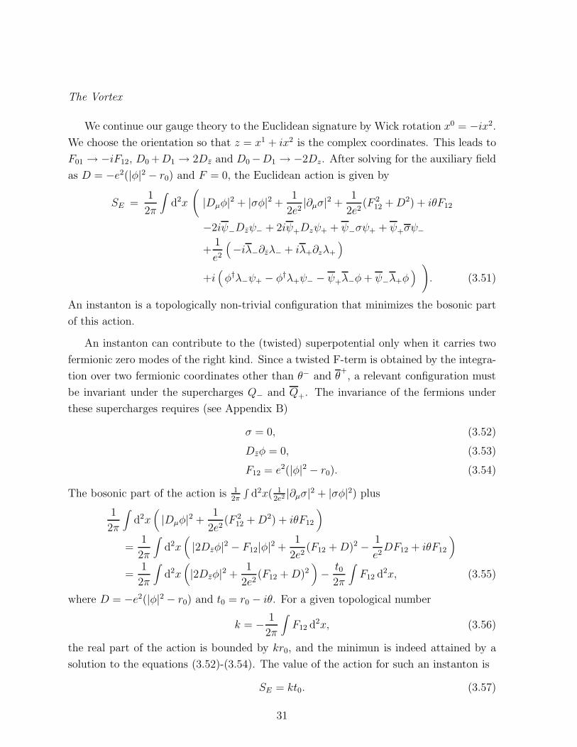
We continue our gauge theory to the Euclidean signature by Wick rotation x0 = −ix2.

We choose the orientation so that z = x1 + ix2 is the complex coordinates. This leads to

F01 → −iF12, D0 +D1 → 2Dz and D0 −D1 → −2Dz. After solving for the auxiliary field

as D = −e2(|φ|2 − r0) and F = 0, the Euclidean action is given by

SE =1

2π

∫d2x

(|Dµφ|2 + |σφ|2 +

1

2e2|∂µσ|2 +

1

2e2(F 2

12 +D2) + iθF12

−2iψ−Dzψ− + 2iψ+Dzψ+ + ψ−σψ+ + ψ+σψ−

+1

e2

(−iλ−∂zλ− + iλ+∂zλ+

)

+i(φ†λ−ψ+ − φ†λ+ψ− − ψ+λ−φ+ ψ−λ+φ

) ). (3.51)

An instanton is a topologically non-trivial configuration that minimizes the bosonic part

of this action.

An instanton can contribute to the (twisted) superpotential only when it carries two

fermionic zero modes of the right kind. Since a twisted F-term is obtained by the integra-

tion over two fermionic coordinates other than θ− and θ+, a relevant configuration must

be invariant under the supercharges Q− and Q+. The invariance of the fermions under

these supercharges requires (see Appendix B)

σ = 0, (3.52)

Dzφ = 0, (3.53)

F12 = e2(|φ|2 − r0). (3.54)

The bosonic part of the action is 12π

∫d2x( 1

2e2 |∂µσ|2 + |σφ|2) plus

1

2π

∫d2x

(|Dµφ|2 +

1

2e2(F 2

12 +D2) + iθF12

)

=1

2π

∫d2x

(|2Dzφ|2 − F12|φ|2 +

1

2e2(F12 +D)2 − 1

e2DF12 + iθF12

)

=1

2π

∫d2x

(|2Dzφ|2 +

1

2e2(F12 +D)2

)− t0

2π

∫F12 d2x, (3.55)

where D = −e2(|φ|2 − r0) and t0 = r0 − iθ. For a given topological number

k = − 1

2π

∫F12 d2x, (3.56)

the real part of the action is bounded by kr0, and the minimun is indeed attained by a

solution to the equations (3.52)-(3.54). The value of the action for such an instanton is

SE = kt0. (3.57)

31

Under the axial rotation by eiα, the path-integral measure in this topological sector

changes by the phase e2ikα. Since the twisted superpotential has axial R-charge 2, we

see that the relevant configurations are those with k = 1.

A solution to (3.53) and (3.54) is the vortex. For each vortex with k = 1, φ has a

single simple zero. The moduli space of gauge equivalence classes of k = 1 vortices is

complex one-dimensional and is parametrized by the location of the zero of φ. To see

this, we note the following well-known fact. The orbit of a solution to (3.53) under the

complexified gauge transformations contains vortex solutions in one gauge equivalence

class, and conversely, any gauge equivalence class of vortex solutions is contained in one

such orbit. Here, a complexified gauge transformation is a rotation (iAz, φ) → (iAz +

h∂zh−1, hφ) by a function h with values in C×. Thus, we only have to find solutions to

the equation Dzφ = 0 modulo the complexified gauge transformations. In other words,

we only have to find pairs of a holomorphic line bundle with a holomorphic section.

Here, it is convenient to compactify our Euclidean 2-plane to a Riemann sphere. Then,

there is a unique holomorphic line bundle of k = 1. Such a bundle has two-dimensional

space of holomorphic sections, where each section has a single simple zero. The residual

complexified gauge symmetry is a multiplication by a constant and it does not change

the location of the zero of a section. Thus, the space of equivalence classes is complex

one-dimensional and is parametrized by the zero locus of φ.

Let us examine in more detail the behaviour of a vortex solution. We consider the

vortex at z = 0. For the finiteness of the action, |φ| must approach the vacuum value

|φ|2 = r0 at infinity. By rescaling φ =√r0φ where |φ| → 1 at infinity, it becomes clear

that the equations depend only on one length parameter 1/e√r0. This characterizes the

size of the vortex. Thus, we expect that the gauge field is nearly flat on |z| ≫ 1/e√r0 and

φ is nearly covariantly constant there. Since (−1/2π)∫F12 = 1, we have Aµ = −∂µ arg(z)

and φ =√r0z/|z| at infinity. The exact solution takes the form

iA = −1 − f

2

(dz

z− dz

z

), (3.58)

φ =√r0 exp

(−∫ ∞

|z|2

dwf(w)

2w

)z

|z| , (3.59)

where f is a function of w = |z|2 which satisfies the equation wf ′′ = e2r0

2f + ff ′ and

the boundary condition f(0) = 1, f(+∞) = 0. The asymptotic behaviour of the function

f(|z|2) at |z| ≫ 1/e√r0 is

f = const√m|z| e−m|z| + · · · , (3.60)

32

where const is a numerical constant and

m = e√

2r0. (3.61)

The vortex at z = z0 is obtained from the above solution simply by the replacement

z → z − z0.

Fermionic Zero Modes

Now let us examine the fermionic zero modes in the instanton background. Since

σ = 0 in this background, the fermionic part of the action (3.51) decomposes into two

parts as

−i(ψ−, λ+)

2Dz −φ

φ† − 1e2∂z

(ψ−

λ+

)+ i(ψ+, λ−)

2Dz −φ

φ† − 1e2∂z

(ψ+

λ−

)(3.62)

Using the index theorem of [67], one can see that the operators of the first and the second

terms have index 1 and −1 respectively in our background. Furthermore, there is no

normalizable zero modes for (ψ−, λ+) nor (ψ+, λ−). To see this we note that

∫d2z

(∣∣∣2Dzψ+ − φλ−∣∣∣2+ 2e2

∣∣∣φ†ψ+ − 1

e2∂zλ−

∣∣∣2)

(3.63)

=∫

d2z(|2Dzψ+|2 + 2e2|φ|2|ψ+|2 +

2

e2|∂zλ−|2 + |φ|2|λ−|2

)(3.64)

in the vortex background, where ψ+ and λ− are considered here as commuting spinors.

The left hand side vanishes for a zero mode of (ψ+, λ−), but then vanishing of the right

hand side requires ψ+ = λ− = 0. The argument for (ψ−, λ+) is the same.

Thus, each of (ψ−, λ+) and (ψ+, λ−) has exactly one zero mode. Actually, the expres-

sion for the zero mode in terms of the vortex solution is available;

ψ

(0)−

λ(0)

−

=

Dzφ

F12

,

ψ

(0)

+

λ(0)+

=

Dzφ

†

F12

. (3.65)

It is easy to verify using the vortex equations (3.53) and (3.54) that these are indeed

the zero modes. These come from the supersymmetry transformation under the broken

supercharges Q− and Q+. The asymptotic behaviour of φ†ψ(0)− and ψ

(0)

+ φ are

φ†ψ(0)− = ∂z|φ|2 = const × r0

z

|z|

√m

|z|e−m|z| + · · · (3.66)

ψ(0)

+ φ = ∂z|φ|2 = const × r0z

|z|

√m

|z|e−m|z| + · · · , (3.67)

33

for the vortex at z = 0. These agree with the asymptotic behaviour of the propagators

for a Dirac fermion of mass m = e√

2r0;

φ†ψ(0)− ∝ r0 S

F−−(z), ψ

(0)

+ φ ∝ −r0 SF++(z). (3.68)

This is not an accident; After a suitable similarity transformation, the operators in (3.62)

near infinity (where φ =√rz/|z| and Aµ = −∂µ arg(z)) become nothing but the Dirac

operator for a free fermion of mass m = e√

2r.

The Computation

In order to prove the generation of e−Y term in the twisted superpotential, we would

like to compute a quantity that is non-vanishing only when such a term is generated. To

find out what is the appropriate object to look at, let us return to our theory of Σ and

Y . We recall that the Lagrangian is

L =∫

d4θ(− 1

2e2ΣΣ − 1

4r0Y Y

)+

1

2

( ∫d2θ

(Σ(Y − t) + cµ e−Y

)+ c.c.

), (3.69)

and we were asking whether c is zero or not. Here we have approximated the Kahler

potential for Y by the one in the continuum limit (3.25).

This theory involves a U(1) gauge field. However, there is no charged field and the

only appearance of the gauge field is in the kinetic term and in the Theta term (with the

Theta angle being ϑ−θ where ϑ = −Im(y)). As is well known [68], the effect of the gauge

field is to generate a mass term for ϑ:

U =e2

2

(˜ϑ− θ

)2, (3.70)

where (α)2 = min(α+2πn)2|n ∈ Z. Thus, we can treat Σ as an ordinary twisted chiral

superfield which has a complex auxiliary field. In particular, the theory without e−Y term

is a free theory of two twisted chiral multiplets. It is easy to diagonalize the ΣY mixing

and it turns out that the combinations X(±) = ±Σ/(2e)+(Y − t)/(2√2r0) are superfields

of mass

±m = ±e√

2r0. (3.71)

Now, it is easy to see that the fermionic components χ+ and χ− of Y has vanishing two

point function in the free theory;

〈χ+(x)χ−(y)〉 = 0, if c = 0. (3.72)

34

However, if e−Y is generated, the twisted F-term would contain a term −e−yχ+χ− in the

Lagrangian. This would contribute to the two point function as

〈χ+(x)χ−(y)〉 = cµr20

∫d2z e−t SF

++(x− z)SF−−(z − y) (3.73)

where SFαβ(x− y) is the Dirac propagator for the fermions of mass m = e

√2r0.

Now, let us compute the two point function 〈χ+(x)χ−(y)〉 in the original gauge theory.

We recall from (3.21) that

χ+ = 2ψ+φ, χ− = −2φ†ψ−. (3.74)

Since the product of these carries an axial R-charge 2, only the vortex backgrounds with

k = 1 can contribute to the two point function. The contribution is expressed as an

integration over the location z of the vortex

〈χ+(x)χ−(y)〉 = −4ΛUV

∫d2z e−t0

(ψ

(0)

+ φ(z)

)(x)

(φ†

(z)ψ(0)−

)(y), (3.75)

where φ(z) is the vortex solution at z. The factor of ΛUV comes from the measure of

bosonic zero modes (∝ Λ2UV ) and that for the fermionic zero modes (∝ Λ−1

UV ). As we have

seen, the fermionic zero mode multiplied by φ is proportional to the Dirac propagator

(3.68). Thus, we obtain

〈χ+(x)χ−(y)〉 = const × r20ΛUV

∫d2z e−t0 SF

++(x− z)SF−−(z − y), (3.76)

which agrees with (3.73) considering the relation ΛUV e−t0 = µ e−t. Thus, we have shown

that our dual theory correctly reproduces the gauge theory result if and only if c 6= 0.

3.2.3 Solitons and Dualization

In the R → 1/R duality, as reviewed before, the momentum and winding modes get

exchanged. This view provides us with another way to interpret the generation of super-

potential (3.50). Let us turn off the gauge interaction and consider Σ as a non-dynamical

parameter. Before dualization, we have a field Φ of mass Σ. In the dual description Φ

should arise as a winding mode. Indeed if we consider the superpotential

W = Σ(Y − t) + e−Y . (3.77)

Viewing Σ as non-dynamical, the vacua are labeled by ∂YW = 0 and we obtain

∂YW = 0 → e−Y = Σ (3.78)

35

and the critical points are given by

Yn = Y0 + 2nπi (3.79)

where Y0 is a special solution of (3.78). The vacua are indexed by an integer |n〉, corre-

sponding to winding number in the Y plane. This should correspond to momentum mode

in the Φ variable. In other words the Φ field should have Y -winding number charge +1

and acts on vacua

Φ : |n〉 → |n+ 1〉 (3.80)

In other words Φ should be identified with the soliton interpolating between the vacua.

The BPS mass in this sector is given by [69]

|m| =1

2π|W (Yn) −W (Yn−1)| = |Σ|, (3.81)

in agreement with the expected mass of Φ. This reasoning provides another view point

on the superpotential in the actual gauge system. Related ideas were recently discussed

in [70].

3.3 A Few Generalizations

It is straightforward to extend the description using the dual fields to more general

gauge theories. We consider here two generalizations; the case with U(1)k gauge group

and the case with twisted masses.

Many U(1) Gauge Groups

The first example is U(1)k gauge group with N matter fields. We denote the field

strength superfield for the a-th gauge group by Σa (a = 1, . . . , k), and the chiral superfield

for the i-th charged matter by Φi (i = 1, . . . , N). We denote by Qia the charge of the i-th

matter under the a-th gauge group.

The exact twisted superpotential can be obtained by the localization argument which

reduces the problem to the sum of copies of the single flavor case. This time, instead of

keeping only one gauge coupling we keep k of them. We start with the sum of N copies of

U(1) theory with charge 1 matter, and take the weak coupling limit except for the U(1)k

gauge group embedded in U(1)N according to the charge matrix Qia. This constrains the

N gauge fields as

Σi =k∑

a=1

QiaΣa. (3.82)

36

The exact superpotential for Σa’s and the dual Yi of Φi is then given by

W =k∑

a=1

Σa

(N∑

i=1

QiaYi − ta

)+ µ

N∑

i=1

e−Yi. (3.83)

Integrating over Yi’s, we obtain the following effective twisted superpotential for Σa’s:

Weff (Σa) = −k∑

a=1

Σa

(N∑

i=1

Qia

(log( k∑

b=1

QibΣb/µ)− 1

)+ ta

). (3.84)

This is the effective superpotential that we would obtain if we integrate out Φi’s in the

original gauge theory [65].

Twisted Masses

The next example is U(1)k gauge theory with N charged matter fields as above, but

the twisted masses mi for the matter fields are turned on. The twisted mass can be

considered as the lowest components of the field strength superfields of the U(1)N/U(1)k

flavor symmetry group. This is a non-trivial deformation of our gauge theory. The

(anomalous) axial R-symmetry is explicitly broken by this perturbation but is restored if

mi are rotated as mi 7→ e2iαmi.

As noted before, the dualization for this case follows from extending the U(1)k gauge

group to U(1)N and taking the suitable decoupling limit. With the twisted masses, the

constraint on the field strengths (3.82) is shifted as

Σi =k∑

a=1

QiaΣa − mi. (3.85)

The exact twisted superpotential is thus

W =k∑

a=1

Σa

(N∑

i=1

QiaYi − ta

)+ µ

N∑

i=1

e−Yi −N∑

i=1

miYi. (3.86)

Note that the net number of deformation parameters is (N − k) from the flavor group

U(1)N/U(1)k; δmi =∑k

a=1Qiaca is absorbed by a shift of the origin of Σa’s. Integration

over Yi’s yields an effective superpotential for Σ that we would obtain if we integrate out

Φi’s in the original gauge theory (as is done in [71] for k = 1 case with Qi = ±1).

4 Sigma Models From Gauge Theories

The gauge theory studied in the previous section reduces at low enough energies to

the non-linear sigma model on a certain manifold. To see this, we examine the space of

37

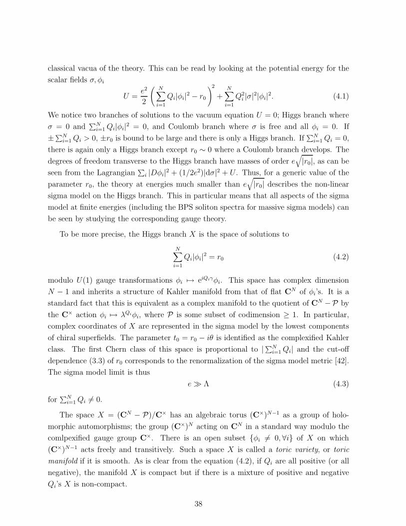
classical vacua of the theory. This can be read by looking at the potential energy for the

scalar fields σ, φi

U =e2

2

(N∑

i=1

Qi|φi|2 − r0

)2

+N∑

i=1

Q2i |σ|2|φi|2. (4.1)

We notice two branches of solutions to the vacuum equation U = 0; Higgs branch where

σ = 0 and∑N

i=1Qi|φi|2 = 0, and Coulomb branch where σ is free and all φi = 0. If

±∑Ni=1Qi > 0, ±r0 is bound to be large and there is only a Higgs branch. If

∑Ni=1Qi = 0,

there is again only a Higgs branch except r0 ∼ 0 where a Coulomb branch develops. The

degrees of freedom transverse to the Higgs branch have masses of order e√|r0|, as can be

seen from the Lagrangian∑

i |Dφi|2 + (1/2e2)|dσ|2 + U . Thus, for a generic value of the

parameter r0, the theory at energies much smaller than e√|r0| describes the non-linear

sigma model on the Higgs branch. This in particular means that all aspects of the sigma

model at finite energies (including the BPS soliton spectra for massive sigma models) can

be seen by studying the corresponding gauge theory.

To be more precise, the Higgs branch X is the space of solutions to

N∑

i=1

Qi|φi|2 = r0 (4.2)

modulo U(1) gauge transformations φi 7→ eiQiγφi. This space has complex dimension

N − 1 and inherits a structure of Kahler manifold from that of flat CN of φi’s. It is a

standard fact that this is equivalent as a complex manifold to the quotient of CN −P by

the C× action φi 7→ λQiφi, where P is some subset of codimension ≥ 1. In particular,

complex coordinates of X are represented in the sigma model by the lowest components

of chiral superfields. The parameter t0 = r0 − iθ is identified as the complexified Kahler

class. The first Chern class of this space is proportional to |∑Ni=1Qi| and the cut-off

dependence (3.3) of r0 corresponds to the renormalization of the sigma model metric [42].

The sigma model limit is thus

e≫ Λ (4.3)

for∑N

i=1Qi 6= 0.

The space X = (CN − P)/C× has an algebraic torus (C×)N−1 as a group of holo-

morphic automorphisms; the group (C×)N acting on CN in a standard way modulo the

comlpexified gauge group C×. There is an open subset φi 6= 0, ∀i of X on which

(C×)N−1 acts freely and transitively. Such a space X is called a toric variety, or toric

manifold if it is smooth. As is clear from the equation (4.2), if Qi are all positive (or all

negative), the manifold X is compact but if there is a mixture of positive and negative

Qi’s X is non-compact.

38

For∑N

i=1Qi = 0, the FI parametr r = r0 does not run and t = r−iθ is a free parameter

of the theory. At r = 0, X contains a singular point φi = 0 where the U(1) gauge group is

unbroken. A new flat direction (Coulomb branch) develops there and the sigma model on

X becomes singular. The actual singularity is determined by the vanishing of the quantum

effective potential at large values of σ. Since there is an effective superpotential Weff (σ)

(3.39) which is valid at large σ, this is equivalent to the condition that ∂σWeff (σ) = 0 at

large values of σ. Thus, singularity of the quantum theory is located at

t = −N∑

i=1

Qi log(Qi). (4.4)

Note that the theory is singular only for a particular value of θ (either 0 or π) and r. In

particular, the theories with r ≫ 0 and r ≪ 0 are smoothly connected to each other [10],

even though the space X at r ≫ 0 differs from X at r ≪ 0.

One can also consider abelian gauge theory with gauge group U(1)k and N matter

fields with N×k charge matrixQia. For a generic value of ta in a certain range, the vacuum

manifold is a Kahler manifold X of dimension N − k. X as a complex manifold is of the

type (CN − P)/(C×)k where P is a union of certain planes in CN . The algebraic torus

(C×)N−k = (C×)N/(C×)k acts on X in an obvious way as holomorphic automorphisms

andX contains an open subset on which (C×)N−k acts freely and transitively. Thus, X is a

toric variety. (In fact, any normal toric variety is obtained this way). We refer the physics

reader to [65] for more precise definition of a toric variety and its general properties. See

also [72, 73] for more detail. If∑N

i=1Qia = 0 for all a, the theory is parametrized by k

dimensionless parameters ta = ra − iθa. Otherwise, there is a single scale parameter and

k − 1 dimensionless parameters. Unlike in the single U(1) case, the theory can possibly

become singular at some locus even if∑N

i=1Qia 6= 0. Singular locus in the parameter

space is determined by finding a flat direction in the σa space; ∂σaWeff = 0 where Weff is

given in (3.84) (more precisely, we must consider all possible “mixed branches” and do the

same computation in the reduced theory). This was studied in detail in [65]. However,

as in the single U(1) case, two generic points in the parameter space can be smoothly

connected to each other without meeting a singularity.

The first Chern class c1(X) of X is not necessarily positive semi-definite. In the

present paper, we only consider X with c1(X) ≥ 0. In such a case, the running of the

FI parameter of the gauge theory matches the running of the sigma model coupling at

one-loop level, and our gauge theory indeed describes the non-linear sigma model on X

at energies well below the gauge coupling constants. To be more precise, the precise

relation of the parameters is possibly complicated when c1(X) is close to zero and the

one-loop running is not dominant. This can also be understood by comparing the size

39

of the moduli spaces of gauge theory instantons and instantons of the non-linear sigma

model (as shown in [10] in the case of projective hypersurfaces). It was also noted in [74]

that the formal parameters corresponding to irrelevant deformations are in complicated

relation even when c1 is large. The precise relation can be determined by finding the

so called flat coordinates with the expansion point at infinity. That would lead to the

natural coordinates used in the large volume expansion of the non-linear sigma model [75].

(This in particular applies to the mirror QFTs that we will obtain later in this paper in

finding the map between the parameters of the non-linear sigma model and the mirror.)

If there is a negative component in c1(X), the sigma model is not asymptotic free and is

not well-defined. In such a case, our gauge theory has little to do with the manifold X.

If c1(X) is negative definite, it is infra-red free and the sigma model (defined as a cut-off

theory) flows to a free theory of c/3 = dimX.

4.0.1 Examples of Toric Varieties

Let us consider some examples of toric varieties. If we consider a U(1) gauge theory with

N fields with charges +1, this gives a linear sigma model realization of CPN−1. More

generally, if the charges of the matter fields are positive but not necessarily equal, it gives

a realization of weighted projective space, with weights determined by the charges.

If we consider a U(1) gauge theory with N fields with charge +1 and one with charge

−d, this gives a realization of the total space of the O(−d) line bundle over CPN−1.

Hirzebruch surface Fa (a = 0, 1, . . .) is a toric manifold of dimension two which is

realized as the vacuum manifold of the U(1) × U(1) gauge theory with four chiral fields

with charges (1, 0), (1, 0), (0, 1), and (a, 1). F0 is the product CP1 × CP1 and F1 is the

blow up of CP2 at one point. The first Chern class is positive for these two cases and it is

positive-semi-definite for F2. In all these cases, the gauge theory describes the non-linear

sigma model. For a ≥ 3, however, c1(Fa) is not even positive semi-definite and the sigma

model is not well-defined.

4.0.2 Holomorphic Vector Fields and Deformations of Linear Sigma Model

The unitary subgroup U(1)N−k of the holomorphic automorphism group (C×)N−k is ac-

tually an isometry group of the Kahler manifold X. Since it is an abelian group, as

explained in section 2, we can use this to deform the sigma model on X by a potential

term like (2.26). One may be interested in whether the deformation can be realized in the

gauge theory. In fact, this U(1)N−k is a commutative subgroup of the flavor symmetry

40

group of the gauge theory, and we can consider the deformation by twisted masses. By

construction, the potential deformation of the sigma model is naturally identified as the

twisted mass deformation of the gauge group. One can also confirm this by computing

the bosonic potential in gauge theory and by checking that it agrees with the potential12|mAVA|2 + 1

2|mAVA|2 from the holomorphic isometry (where VA are the generators of

U(1)N−k). We exhibit this in the simplest case X = CP1 and leave the general case as an

exercise. The CP1 sigma model is realized by a U(1) gauge theory with two fields Φ1 and

Φ2 of unit charge. The potential of the gauge theory with the twisted mass is given by

U =e2

2(|φ1|2 + |φ2|2 − r)2 + |σ − m|2|φ1|2 + |σ|2|φ2|2. (4.5)

We now fix φ1 and φ2 to lie in the CP1 before perturbation (|φ1|2 + |φ2|2 = r) and then

extremize the potential with respect to σ. Plugging the result back into (4.5), we obtain

the potential

Um =|m|2r

|φ1|2|φ2|2. (4.6)

On the other hand, the U(1) isometry generates a holomorphic vector field with V z =

iz∂/∂z where z is the coordinate of CP1 given by z = φ1/φ2. The metric of CP1 de-

termined by the quotient is the standard Fubini-Study metric ds2 = r|dz|2/(1 + |z|2)2.

Measuring V by this, we obtain the potential

|m|2 ‖ V ‖2= |m|2 r|z|2(1 + |z|2)2

= |m|2 |φ1|2|φ2|2r

(4.7)

which is nothing but (4.6).

4.1 Hypersurfaces and Complete Intersections

The non-linear sigma models of hypersurface or complete intersections in a compact

toric manifold can also be realized as a gauge theory [10]. Let X be the compact toric

manifold realized as the vacuum manifold of U(1)k gauge theory with N matter fields Φi

of charge matrix Qia. We shall consider the submanifold M of X defined by the equations

Gβ = 0, β = 1, . . . , l, (4.8)

where Gβ are polynomials of Φi of charge dβa for the a-th U(1) gauge group. Let us add

l matter fields Pβ of charge matrix −dβa to the U(1)k gauge theory. This theory by itself

realizes a non-linear sigma model on a non-compact toric manifold V . V is the total space

of the sum of l line bundles on X; The new coordinates pβ parametrize the fibre directions

and X is embedded in V as the zero section pβ = 0. Now let us consider the gauge theory,

41

with the same gauge group and the same matter content, but having a gauge invariant

superpotential of the form

W =l∑

β=1

PβGβ(Φ). (4.9)

Then, the vacuum equation requires Gβ = 0 and∑

β pβ∂iGβ = 0. If M is a smooth

complete intersection in X, this means that pβ = 0 for all β and the vacuum manifold

is M itself. Thus, the gauge theory with the superpotential (4.9) realizes the non-linear

sigma model on the complete intersection M in X.

Thus the sigma model on the compact manifold M is closely related to the sigma

model on the non-compact toric manifold V . In fact they both have the same gauge field

and matter content. The only difference between them is that, in the compact theory,

there is an F-term involving a gauge invariant superpotential W which yields cc ring

deformation. In this sense the compact theory can be embedded in the non-compact

theory. The non-compact theory is obtained by considering W → ǫW in the limit of

setting ǫ → 0. Of course this limit changes drastically the behavior of the theory and in

particular the theory has 2l more complex dimensions in the UV.

However, we can ask if there are any quantities which are unaffected by this defor-

mation. The answer is that if we are considering quantities (such as ac ring) which are

sensitive only to the twisted F-terms such as Kahler parameters (the FI terms of the

gauge theory), then they should not depend on the F-term deformations. Thus for those

questions it should be irrelevant whether we are considering the compact theory or the

non-compact theory. All that we have to do is to find out how the states and the opera-

tors of the compact theory are embedded in that of the non-compact theory and compute

the protected quantities that way. This is in fact analogous to embedding questions of

vacuum geometry from one theory in a theory of higher central charge, discussed in [26].

It is also similar to the computation of the elliptic genus of minimal models using a free

theory with higher central charge [76].

In the present case this issue has been studied in [65] where they also obtain the

embedding of the chiral field of the sigma model on M theory with that of V . This result

is stated as follows. Let δβ (β = 1, . . . , l) be the ac ring element of the theory on V defined

by

δβ =k∑

a=1

dβaΣa, (4.10)

where Σa is the field strength of the a-th gauge group. Then, the correlation functions

〈...〉M of the A-twisted model on M are obtained from those 〈...〉V on V by

〈O1 · · ·Os〉M = 〈O1 · · ·Os(−δ21) · · · (−δ2

l )〉V . (4.11)

42

An intuitive understanding of this relation is available in the quantum mechanics obtained

by dimensional reduction. Let La be a line bundle over V defined by the equivalence rela-

tion (pβ, φi; c) ≡ (∏

a λ−dβaa pβ,

∏a λ

Qiaa φi;λac) where (λa) is the element of the complexified

gauge group (C×)k and c is the fibre coordinate. Then, one can show that the ac ring

element Σa corresponds to the first Chern class c1(La) of La. Now, let us consider the

tensor product

Lβ =k⊗

a=1

L⊗dβaa , (4.12)

whose first Chern class corresponds to the ac ring element δβ. The line bundle L−1β has

a section proportional to pβ and thus −δβ represents the divisor class of pβ = 0 in V . In

particular, the product (−δ1) · · · (−δl) represents the class X in V . On the other hand,

the bundle Lβ has a section proportional to Gβ and thus δβ represents the divisor class

of Gβ = 0. Therefore, (−δ21) · · · (−δ2

l ) represents a delta function supported on M . What

is shown in [65] is basically that this quantum mechanical interpretation remains true for

the full 2d QFT as long as topological correlators are concerned. It turns out that we need

a stronger version of the relation (4.11). We thus proceed to a physical derivation of this

relation, which uses the fact that the compact and non-compact theories are embedded

in the same underlying physical theory, and yields the stronger version that we need.

The basic idea is that with ǫ 6= 0 we have turned on a superpotential and we can

follow the states from the non-compact theory to the compact theory. In this sense the

non-compact theory flows in the IR limit (for non-vanishing ǫ) to the compact theory. We

can thus follow the states in the non-compact theory and ask which ones survive in the IR

limit. By the nature of the RG flow, we will be losing some states as we take the IR limit.

However, if we concentrate on the ground states in the Ramond sector which correspond

to normalizable states in the non-compact theory, then in the compact theory they are

bound to survive as a ground state (the same cannot be said of the non-normalizable

ground states in the non-compact theory, which might disappear from the spectrum of

the compact theory).

In the sigma model on the non-compact manifold V , the ground state corresponding

to the operator δ = δ1 · · · δl is a normalizable state which is the product of Kahler forms

that control the sizes of the compact part of the geometry. We denote this state by

|δ〉V . (4.13)

In the large volume limit, this state has the axial R-charge − dimC V + 2l = − dimCM

which is the lowest among normalizable ground states. Now, let us turn on the super-

potential ǫW where W is the one given in (4.9). The state |δ〉V which is the unique

43

normalizable ground state in the Ramond sector with axial charge − dimC V + 2l will be

deformed to a state which we denote by |δ〉ǫ. By standard supersymmetry arguments, this

state is a normalizable ground state of the Ramond sector. For large ǫ (or for any finite

ǫ in the IR limit) the theory corresponds to the sigma model on the compact manifold

M for which there is a unique ground state with axial charge − dimCM , which is also

sometimes denoted by |1〉M . Thus we can identify |δ〉ǫ = |1〉M as long as axial charge is

conserved. Thus, we have the following correspondence of states as we increase ǫ;

|δ〉V ǫ 6=0−→ |δ〉ǫ ǫ→∞−→ |1〉M . (4.14)

Here we have used the axial R-charge to identify the state to which |δ〉V is deformed.

For the more general case, where the axial R-sysmmetry is broken by an anomaly, the

result still remains true, as we will now argue. To see this, note that at large Kahler

parameters, i.e. as ta → ∞ axial R-charge is a good symmetry. So at least to leading

order it is correct. To show it is true for all ta we proceed as follows: According to [57] the

topologically twisted theory picks a section of the vacuum bundle which is holomorphic

in the sense defined by the topological twisting. In particular we can choose the pertubed

state |δ〉ǫ so that∂

∂ta|δ〉ǫ = 0. (4.15)

For infinitely large ta, since the axial charge is conserved the state |δ〉V is deformed for

finite ǫ to |1〉M . For finite but large ta the fact that we can choose a holomorphic section

of the vacuum bundle shows that the difference between |δ〉ǫ and |1〉M can only be given

by states with coefficients involving some powers of qa = e−ta . Here we note that the

axial R-charge can be made conserved by shifting the Theta angle to cancell (3.4). This

in particular means that we assign non-negative R-charges to qa as long as the first Chern

class of M is positive-semi-definite. It thus follows that qa’s would be accompanied by

states which will have too small an R-charge to correspond to a normalizable state, since

|δ〉V is the unique normalizable ground state with minimum R-charge. This establishes

the relation (4.14) in general.

The relation (4.14) can be used to yield another derivation of the relation (4.11): The

topological correlations for sigma model on M can be written as

〈O1 · · ·Os〉M = 〈1|O1 · · ·Os|1〉M = 〈δ|O1 · · ·Os|δ〉V = 〈(−δ21) · · · (−δ2

l )O1 · · ·Os〉V .(4.16)

where we have used the ǫ independence in the topologial A-model computations, as ǫW

does not affect the ac correlation functions (note that the overall proportionality factor is

not fixed, and depends on the choice of normalization of the topologically twisted theory).

44

4.1.1 Examples of Hypersurfaces

Consider a U(1) gauge theory with N fields Φi of charge +1 and one field P with charge

−d. So far this is the same as the linear sigma model description of the total space of the

line bundle O(−d) over CPN−1. However, now consider adding to the action the F-term

with superpotential

W = PG(Φi) (4.17)

where G is a polynomial of degree d in Φi. This gauge theory describes, in the infrared,

the sigma model on a hypersurface of degree d in CPN−1. The hypersurface for d = N is

a Calabi-Yau manifold of complex dimension N −2. For d < n it is a manifold of positive

c1 and the sigma model is asymptotically free. For d > n it is a manifold with negative

c1 and the sigma model is not asymptotically free.

The geometric regime corresponds to when the FI parameter is very large r ≫ 0

(which is the UV limit for d < N). If we consider the limit r → −∞ (which is the IR

limit for d < N), we end up with an LG theory [10]: P picks up an expectation value

and breaks the U(1) gauge symmetry to a discrete subgroup Zd and the effective theory

is given by the LG model with W = G(Φi) divided by a Zd action, which corresponds to

multiplying the fields Φi by a d-th root of unity. If we turn off the superpotential, i.e.,

back in the non-compact toric model corresponding to the total space of the line bundle

O(−d) over CPN−1 the limit r → −∞ would correspond to the orbifold of the free theory

of N fields Φi modded out by Zd, acting as the d-th root of unity on Φi.

The generalization of the above to the case of hypersurfaces of weighted projective

space are straightforward.

5 A Proof Of Mirror Symmetry

In this section we show how the results of section 3 on the dynamics of supersymmetric

gauge theories naturally lead to a proof of mirror symmetry. Before embarking on the

proof, we discuss what we mean by the “proof”.

5.1 What We Mean by Proof of Mirror Symmetry

As we have discussed before the action for a (2, 2) supersymmetric field theory has three

types of terms: D-terms, F-terms and twisted F-terms. In the case of a supersymmetric

sigma model, these three types of terms have the following interpretations: The D-terms

correspond to changing the metric on the target manifold without changing the Kahler or

45

complex parameters. For example for CP1 we can consider a fixed total area, but deform

the metric from the round metric to any other metric with the same total area by varying

the D-term. Variations of F-terms and twisted F-terms correspond to deformations of

complex and Kahler parameters of the target space. As discussed before, F-terms and

twisted F-terms control many important aspects of the (2, 2) theories. In particular the cc

and ac rings depend only on F-terms and twisted F-terms respectively and are independent

of D-terms. These in particular encode the instanton corrections of the sigma model to

the ac ring. Also BPS structure of the massive (2, 2) theories are completely determined

by the F-terms and twisted F-terms [57, 26, 78]. One can define the notion of D-branes

for (2, 2) theories (as is familiar in the conformal case, and can be easily extended to the

non-conformal case as we will discuss in section 6). One can also show that the overlap

of the corresponding boundary states with vacua will only depend on the F-terms (or

twisted F-terms depending on which combination of supercharge the D-brane preserves).

These indicate the importance of F-terms and twisted F-terms for the (2, 2) theories.

In fact they become even more prominent in the conformal case, for example for the

case of Calabi-Yau manifolds. Namely in that case the sigma model flows in the infrared

limit to a conformal field theory which is determined entirely by the complex and Kahler

parameters of the manifold. In other words the metric on the Calabi-Yau manifold adjusts

itself to the unique form consistent with conformal invariance for a given Kahler and

complex structure. In particular the D-terms are entirely determined by the F-terms and

twisted F-terms in this case, as far as the IR behavior is concerned. As a consequence, a

deformation of the conformal field theory corresponds to a deformation of the Kahler or

complex structure of the Calabi-Yau manifold, which in turn is realized through variations

of F-terms and twisted F-terms. From these facts, and from the fact that the cc and ac

rings are determined in terms of F-terms and twisted F-terms one wonders whether the

opposite is true (i.e. whether the cc and ac rings determine the F-terms and twisted

F-terms and thus the full theory). This is, however, not completely true; theories with

the same chiral ring can differ in the “integral structure” [77]. More precisely, in order to

completely specify the theory we need to know the structure of the allowed D-branes.

We prove mirror symmetry in two different senses: In the strong sense, we find a

dual theory, for which we prove it is equivalent to the original theory, up to deformations

involving D-terms. In the weak sense, we propose a dual theory for which we can only

show that the cc, ac, BPS structure of solitons and the D-brane structure are the same.

The weak and strong senses become equivalent if we assume that the cc and ac ring,

together with the integral structure determine the theory up to D-term variations.

We are now ready to discuss the proof for mirror symmetry. We divide the discussion

46

into several cases and indicate in each case what is the sense of the proof (strong/weak)

that we shall present.

5.2 The Proof

The cases of interest naturally divide into three different classes:

(i) X = CPN−1 or a more general compact toric manifold with c1(X) ≥ 0,

(ii) X is a non-compact Calabi-Yau or a more general non-compact toric manifold.

And finally,

(iii) Sigma models on hypersurfaces or complete intersection in X.

It turns out that the mirror for the cases (i) and (ii) are rather straightforward to

derive, using the tools we have developed so far and we shall prove them in the strong

sense. For the derivation of the case (iii) we need an additional tool, which we will discuss

in section 6, and we postpone a complete discussion of (iii) to section 7. This will lead to

a proof of case (iii) in the weak sense. In this section after deriving the general mirror for

the cases (i) and (ii) we briefly mention how it effectively gives an answer of the case (iii)

(to be more fully developed in section 7). We present some examples for cases (i) and (ii)

and how it relates to case (iii) to illustrate the meaning of the results.

We first consider the sigma model on a toric manifold which is described by a gauge

theory with a single U(1) gauge group with chiral fields of charge Qi (i = 1, . . . , N). We re-

call that the dual of the gauge theory is described by a vector multiplet with field strength

Σ and N periodic variable Yi dual to the charged matter fields. It has an approximate

Kahler potential (1/2e2)|Σ|2 +∑

i |Yi|2/4r0 and an exact twisted superpotential

W = Σ

(N∑

i=1

QiYi − t(µ)

)+ µ

N∑

i=1

e−Yi . (5.1)

The fields Σ and∑

iQiYi have mass of order e√|r0| while the mass scale for the modes

tangent to∑

iQiYi = t is of order µ√|r0| where µ ∼ Λ for

∑iQi 6= 0. In the sigma model

limit e≫ µ, these mass scales are well-separated and it becomes appropriate to integrate

out Σ. This yields the constraintN∑

i=1

QiYi = t. (5.2)

Clearly this can be solved by N −1 periodic variables. Now, the dual theory becomes the

47

theory of such N − 1 variables solving (5.2) with the twisted superpotential

W = µN∑

i=1

e−Yi. (5.3)

This can be interpreted as a sigma model on (C×)N−1 with a twisted superpotential.

Since the complex coordinates are the lowest components of twisted chiral superfields,

this theory can be identified as the mirror of the non-linear sigma model on X.

It is straightforward to extend this to the more general case where we start with k

U(1) gauge groups and N matter fields of charge Qia (i = 1, . . . , N , a = 1, . . . , k). The

target space X of the sigma model is the quotient of

N∑

i=1

Qia|φi|2 = ra (5.4)

by the U(1)k action φi 7→ eiQiaγaφi, which is a toric variety of dimension N − k. The dual

description of the gauge theory is obtained in (3.83). Integrating out the vector multiplet,

we obtain the algebraic torus (C×)N−k as the solutions to

N∑

i=1

QiaYi = ta. (5.5)

The dual theory is a sigma model on this (C×)N−k with the twisted superpotential

W = µN∑

i=1

e−Yi. (5.6)

This can be identified as the mirror of the sigma model on X. We thus have established

the mirror symmetry of the non-linear sigma model on a toric variety XN−k and the

theory on the algebraic torus (C×)N−k with a superpotential.

We can also consider deforming the sigma model using holomorphic vector fields,

as discussed in section 2. There are (N − k) such parameters corresponding to the

U(1)N/U(1)k holomorphic isometry group for the above toric variety. We parameterize

these deformations by N parameters mi (as we will see below k of them are redundant).

The corresponding gauge theory is the one with the twisted masses mi and the twisted

superpotential for the dual theory is obtained in (3.86). Adding the twisted masses does

not affect the elimination of the field strength Σa and we obtain the same constraints

(5.5). All it does is to shift the superpotential (5.6) as

W = µN∑

i=1

e−Yi −N∑

i=1

miYi. (5.7)

48

This is not a single valued function on (C×)N−k, but the multivaluedness is a constant

shift and therefore the Lagrangian itself is well-defined. It is easy to see, using (5.5) that

k of the parameters mi are redundant and do not affect the superpotential.

We will now illustrate these ideas in two concrete cases: One is in the context of

compact toric varieties which we exemplify by using the case of CPN−1. The second one

is for the case of non-compact toric varieties which we exemplify by considering the total

space of O(−d) line bundle over CPN−1. In the context of the latter example we also

explain briefly how the mirror for the hypersurface case arises. We complete the discussion

for the hypersurface case in section 7.

5.3 Compact Toric Manifold

The CPN−1 Model

The linear sigma model for X = CPN−1 is the U(1) gauge theory with N matter fields

of charge 1. The constraint∑N

i=1 Yi = t is solved by Yi = t/N −Θi (i = 1, . . . , N − 1) and

YN = t/N+∑N−1

i=1 Θi, where Θi are periodic variables of period 2πi and can be considered

as coordinates of (C×)N−1. The superpotential is

W = Λ

(eΘ1 + · · ·+ eΘN−1 +

N−1∏

i=1

e−Θi

), (5.8)

where Λ = µ e−t/N is the dynamical scale of the theory. This is the superpotential for

supersymmetric affine AN−1 Toda field theory. Thus, we have derived the mirror symme-

try of CPN−1 model and affine Toda theory which was observed in [25, 26, 16, 28, 29] from

various points of view.

Having no F-term, the theory is invariant under U(1)V R-symmetry. The twisted

superpotential (5.8) explicitly breaks U(1)A but its Z2N subgroup remains unbroken; for

Θj → Θj + 2πi/N , W → e2πi/NW . The vacua of the theory are given by the critical

points of W , ∂ΘiW = 0. It is solved by eΘ1 = · · · = eΘN−1 =: X where X = X−(N−1).

Namely, there are N vacua at eΘj = e2πiℓ/N (all j) with the critical value

W = NΛ e2πiℓ/N , (5.9)

(ℓ = 0, . . . , N − 1). Each vacuum is massive and breaks spontaneously the axial R-

symmetry Z2N to Z2. All these are indeed the properties which are possessed by the

CPN−1 model.

An advantage of LG type description is that the BPS soliton spectrum can be exactly

analyzed using the superpotential. A BPS soliton corresponds to a trajectory connecting

49

two vacua which projects onto a straight line in the W space. The mass is equal to the

absolute value of the susy central charge which is given by the difference of the two critical

values of W . From (5.9) we see that the BPS soliton connecting the 0-th and the ℓ-th

vacua has central charge

Z0ℓ = NΛ( e2πiℓ/N − 1). (5.10)

One can also see that there are(

Nℓ

)such solitons [79]. For each of them, ℓ of e−Yi are

equal to a trajectory fℓ in C× while the remaining (N−ℓ) of them to another fN−ℓ. They

both starts from e−t/N and ends at e−t/N+2πiℓ/N but fℓ has a relative winding number

(−1) compared to fN−ℓ. Since the winding in Yi is dual to the charge for phase rotation

of Φi, the soliton has the same quantum number as the product Φi1 · · ·Φiℓ . Indeed, the

soliton spectrum of the CPN−1 model has been studied in [61] and it was found that the

ℓ = 1 solitons are the elementary electrons Φi and the higher-ℓ solitons are their ℓ-th

antisymmetric products. This spectrum for the solitons was also recovered from the tt∗

geometry in [80].

We can also consider deforming the CPN−1 sigma model by the addition of a com-

bination of the holomorphic vector fields U(1)N−1. In such a case we obtain the mirror

(5.7):

W = Λ

(eΘ1 + · · ·+ eΘN−1 +

N−1∏

i=1

e−Θi

)+

N−1∑

i=1

(mi − mN)Θi, (5.11)

As has been noted, mi’s changes the central charge of the supersymmetry algebra by a

term proportional to the charges Si of the global abelian symmetry U(1)N−1,

δZ =N−1∑

i=1

(mi − mN )Si. (5.12)

The charges Si can be identified with the weights of the SU(N) global symmetry. In this

way we can recover not only the soliton spectrum, but also their quantum numbers under

the SU(N) global symmetry, and obtain the anticipated result noted above [79]. Note

also, that the above deformation, deforms the quantum cohomology ring. If we denote

by x = −dW/dt the generator of the chiral ring (corresponding to the Kahler class of

CPN−1), from the above superpotential one obtains

N∏

i=1

(x− mi) = ΛN . (5.13)

Note that the twisted masses deforms the cohomologry ring from the simple form xN = ΛN

to an arbitrary polynomial of degree N . The result for the case of CP1 was first derived

through other arguments in [81]. The general case was conjectured in [71] from brane

construction of the theory.

50

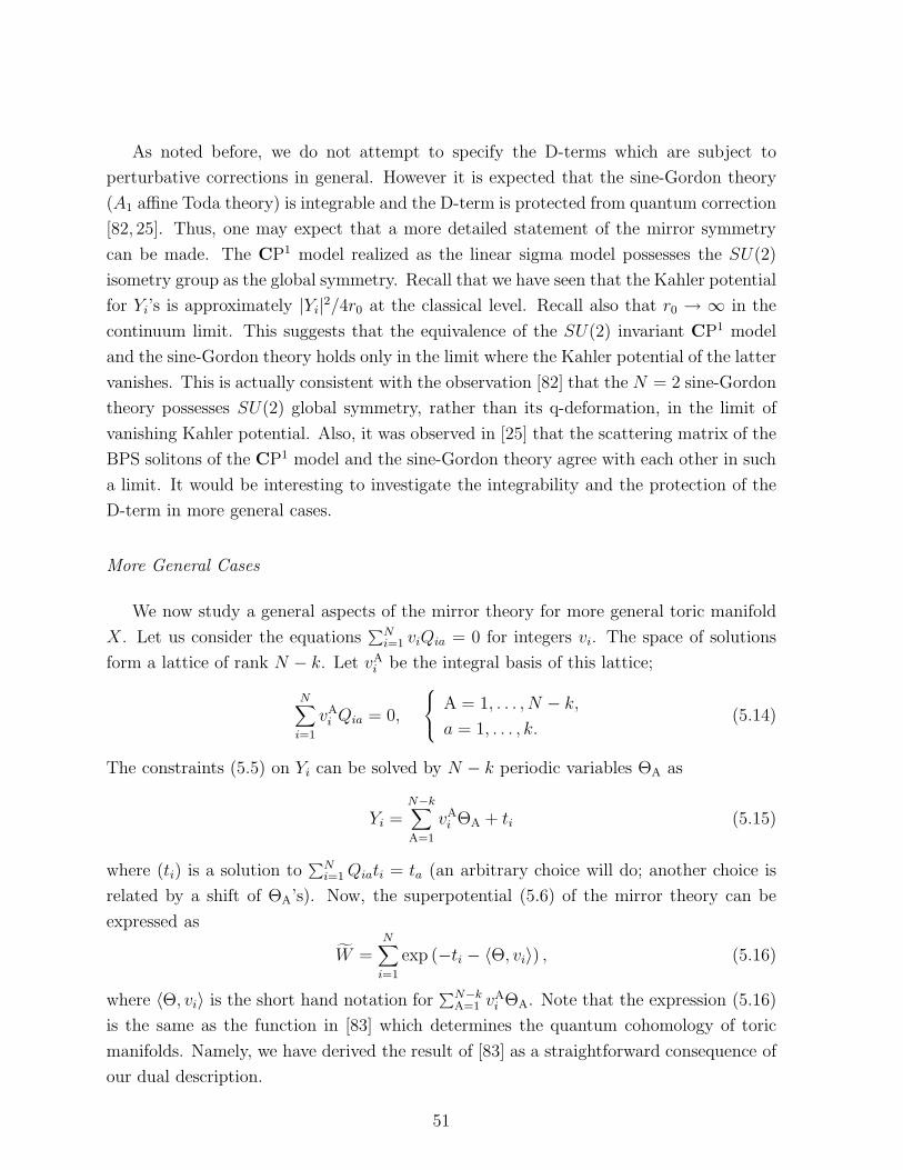
As noted before, we do not attempt to specify the D-terms which are subject to

perturbative corrections in general. However it is expected that the sine-Gordon theory

(A1 affine Toda theory) is integrable and the D-term is protected from quantum correction

[82, 25]. Thus, one may expect that a more detailed statement of the mirror symmetry

can be made. The CP1 model realized as the linear sigma model possesses the SU(2)

isometry group as the global symmetry. Recall that we have seen that the Kahler potential

for Yi’s is approximately |Yi|2/4r0 at the classical level. Recall also that r0 → ∞ in the

continuum limit. This suggests that the equivalence of the SU(2) invariant CP1 model

and the sine-Gordon theory holds only in the limit where the Kahler potential of the latter

vanishes. This is actually consistent with the observation [82] that the N = 2 sine-Gordon

theory possesses SU(2) global symmetry, rather than its q-deformation, in the limit of

vanishing Kahler potential. Also, it was observed in [25] that the scattering matrix of the

BPS solitons of the CP1 model and the sine-Gordon theory agree with each other in such

a limit. It would be interesting to investigate the integrability and the protection of the

D-term in more general cases.

More General Cases

We now study a general aspects of the mirror theory for more general toric manifold

X. Let us consider the equations∑N

i=1 viQia = 0 for integers vi. The space of solutions

form a lattice of rank N − k. Let vAi be the integral basis of this lattice;

N∑

i=1

vAi Qia = 0,

A = 1, . . . , N − k,

a = 1, . . . , k.(5.14)

The constraints (5.5) on Yi can be solved by N − k periodic variables ΘA as

Yi =N−k∑

A=1

vAi ΘA + ti (5.15)

where (ti) is a solution to∑N

i=1Qiati = ta (an arbitrary choice will do; another choice is

related by a shift of ΘA’s). Now, the superpotential (5.6) of the mirror theory can be

expressed as

W =N∑

i=1

exp (−ti − 〈Θ, vi〉) , (5.16)

where 〈Θ, vi〉 is the short hand notation for∑N−k

A=1 vAi ΘA. Note that the expression (5.16)

is the same as the function in [83] which determines the quantum cohomology of toric

manifolds. Namely, we have derived the result of [83] as a straightforward consequence of

our dual description.

51

It is useful to consider vi = (vAi ) as (generically linearly dependent) N vectors in the

lattice N = ZN−k and ΘA as the coordinates on MC = M⊗C where M is the dual lattice

of N. Then, 〈Θ, vi〉 that appears in (5.16) can be identified as the natural pairing. It is

well-known in toric geometry [72, 73] that X is compact if and only if the cone generated

by vi covers the whole NR = N ⊗ R (i.e. any element of NR is expressed as a linear

combination of vi’s with non-negative coefficients). This in particular means that there

is no value of Θ ∈ MC such that Re〈Θ, vi〉 ≥ 0 for all i. In other words, for any non-

zero ReΘ, Re〈Θ, vi〉 < 0 for some i. Thus, there is no obvious run-away direction of the

superpotential (5.16) and we generically expect a discrete spectrum. 1 This is of course

an expected property for a mirror of a compact sigma model.

Since the Witten index of the sigma model is equal to the Euler number

Tr(−1)F = χ(X), (5.17)

the number of critical points of the superpotential (5.16) must agree with χ(X). To check

this, we note another well-known fact in toric geometry: Our algebraic torus (C×)N−k

(with coordinates eΘA) is embedded as an open subset of a “dual” toric variety Y and

each term in (5.16) extends to a section of the anti-canonical bundle K−1Y of Y .2 Thus,

each partial derivative ∂AW = ∂W /∂ΘA also extends to a section sA of K−1Y . Since a

critical point is a common zero of all ∂AW ’s, the number of critical points is the number

of intersection points of the divisors ∂AW = 0 in (C×)N−k. Since there is no run-away

behaviour of the potential for generic values of ta, we do not expect a common zero of

sA’s at infinity Y − (C×)N−k. Thus, the number of critical points must be the same as

the topological intersection number of the N −k divisors sA = 0 in Y which is counted as

Trmirror(−1)F = 〈[Y ], c1(K−1Y )N−k〉. (5.18)

Therefore the number (5.18) must agree with the Euler number of X. It appears that this

is not known in general. However, this certainly holds in every example one can check as

long as c1(X) ≥ 0.

Since the sigma model is well-defined and the gauge theory agrees with it only when

the first Chern class of X is positive semi-definite, the above result makes sense only in

1There can be an accidental situation (which appears in a sublocus of the parameter space) where

there is a run-away direction. This comes from the singularity of the sigma model that is associated with

the development of the Coulomb or mixed branch, which is studied in [65].2The “dual” toric variety is constructed as follows. Take the convex hull of vi’s in NR; this makes a

convex polytope ∆ in NR. Consider the dual ∆ ⊂ MR of ∆ ⊂ NR defined as the set of points in MR

whose values at ∆ are ≥ −1. Then, the vertices uI of ∆ determines the “dual” toric variety Y .

52

such cases c1(X) ≥ 0. To illustrate this, we consider the Hirzebruch surface Fa. As noted

before, the charge matrix for Fa is Qi1 = t(1, 0, 1, a) and Qi2 = t(0, 1, 0, 1) and therefore

the vectors vAi are given by v1 = (1, 0), v2 = (0, 1), v3 = (−1, a) and v4 = (0,−1). Then

the superpotential is given by

W = e−Θ1 + e−t2e−Θ2 + e−t1eΘ1−aΘ2 + eΘ2 . (5.19)

It is easy to see that the number of critical points are 4 for a = 0, 1 and 2a for a ≥ 2.

Since the Euler number of Fa is always 4, the result is “correct” only for a = 0, 1, 2. This

is consistent because c1(Fa) is positive semi-definite only for a = 0, 1, 2.

5.4 Non-Compact Case

In the case where X is non-compact there is an obvious run-away direction of the

superpotential W . To see this, we note that X is non-compact if and only if vi’s generate

a proper convex cone in NR. This means that there is a point Θ0 in MR such that

〈Θ0, vi〉 ≥ 0 for all i. Now, consider the behaviour of the superpotential W at Θ =

tΘ0 in the limit t → +∞. In the case where 〈Θ0, vi〉 > 0 for all i, each term of the

superpotential vanishes in the limit and this is the run-away direction. If there is some i

such that 〈Θ0, vi〉 = 0 the superpotential stays finite but can be extremized by choosing

an appropriate Θ0. In any case, there is a run-away direction of the superpotential. We

thus expect a continuous spectrum, which is indeed a property of the sigma model on a

non-compact manifold.

Below, we present two basic examples of non-compact toric manifolds. The first one,

the total space of O(−d) over CPN−1, provides a starting point of the discussion of the

mirror for hypersurfaces in CPN−1 and more general toric complete intersections. The

second one, the total space of O(−1) ⊕ O(−1) over CP1, is important for the study of

phase transition in the sense of [10, 84].

O(−d) over CPN−1

The linear sigma model for the non-compact space given by the total space O(−d)over CPN−1 is given by a U(1) gauge theory with N fields with charge +1 and one field

with charge −d. As discussed before we find that the mirror for this theory is an LG

theory given by an LG theory with superpotential

W =N∑

i=1

e−Yi + e−YP

53

where

−dYP +N∑

i=1

Yi = t (5.20)

and YP is the dual field to the charge −d matter and Yi for i = 1, ..., N are dual to the

charge +1 matter fields. It is natural to use (5.20) to solve for YP . Let us define

Xi = e−Yi/d (5.21)

for i = 1, ..., N . Then we have

e−YP = et/dX1X2...XN (5.22)

and therefore

W = Xd1 +Xd

2 + ... +XdN + et/dX1X2...XN (5.23)

However, we have to note that the field redefinition (5.21) is not single valued. In fact as

we shift Yi → Yi + 2πi we transform Xi by a primitive d-th root of unity

Xi → Xie−2πi/d.

However, from (5.22) we see that the product of the Xi is well defined. Thus the LG

theory we get is given by the above superpotential W modded out by G = (Zd)N−1 where

G is the group which acts on Xi by all d-th roots of unity which preserve the product

X1X2...XN .

As we discussed in section 4, the linear sigma model for the above non-compact the-

ory and the one given by a hypersurface of degree d in CPN−1 differ by deformations

involving only the cc ring elements, which thus do not affect the ac ring, which we are

studying through mirror symmetry. Thus we expect the same LG with superpotential

(5.23) (modded out by G) to describe the mirror of hypersurface of degree d in CPN−1.

Note that for the case of Calabi-Yau manifolds d = N , and this gives the mirror con-

struction of Greene and Plesser [4]. However clearly there should be a difference between

non-compact case and the compact theory. For example their conformal central charges

(in N = 2 units) differ by 2 in the Calabi-Yau case. What we will find is that indeed

there is a difference and this is reflected in what is the appropriate field variable. In the

compact case (i.e. the hypersurface case) we will find that the fundamental fields are Xi,

whereas in the non-compact case the fundamental fields are Yi which are related to Xi as

defined in (5.21). This will be discussed after our discussion of the realization of D-branes

in LG theories and their associated “BPS masses”.

54

O(−1) + O(−1) over CP1

As a special case of interest, which has been studied in [10] let us consider the mirror

for O(−1) +O(−1) over CP1. This is given by the linear sigma model with a single U(1)

with four fields with charges (−1,−1,+1,+1). For non-vanishing t we can eliminate Σ as

before and we obtain, in the dual formulation the superpotential

W = X1 +X2 +X3 +X4

with Xi = e−Yi and

X1X2 = X3X4et.

We can eliminate, say X1 and write

W = X2 +X3 +X4 + etX3X4/X2

Later in this paper we will return to this example and show how the prepotential for this

model (i.e., the famous tri-logarithmic structure of [11, 85]) can be obtained using the

mirror potential we have found here.

6 D-branes, BPS Mass and LG Models

In the case of Calabi-Yau manifolds one can consider special n-dimensional Lagrangian

submanifolds, and they represent a class in Hn(M). We can imagine a D-brane wrapping

that class. In the sigma model we consider worldsheet with boundaries where the bound-

ary can end on these manifolds. Such boundaries preserve the A-model supercharges.

Given the fact that the neutral observables of the B model correspond to n-form (after

contraction with the holomorphic n-form) we have a natural pairing between B-model

chiral fields, and A-model boundary states. The pairing is simply given by integrating

the corresponding n-form on the corresponding n-cycle. Moreover, this integration can

also be interpreted as the inner product of the boundary state defined by the D-brane

and state defined (through topological twisting) by the B-model observable [86]. In other

words

〈γi|φα〉 =∫

γi

φα

where γi represents an n-dimensional cycle giving rise to boundary state 〈γi| and φα

represents an element of the B-model chiral field corresponding to an n-form. There is

one distinguished element for the chiral ring, the identity operator, which corresponds to

the holomorphic n-form Ω on the Calabi-Yau. In particular we have

Zi = 〈γi|1〉 =∫

γi

Ω

55

For type IIB compactifications on Calabi-Yau 3-folds, the Zi also represents central ex-

tension of supersymmetry algebra, in a sector with D-brane wrapping the γi cycle.

In the context of LG models, the natural topological theory corresponds to the B-

model one [56]. It is thus natural to ask the analog of this pairing in the context of the

LG models. This is important in our applications because we have found an equivalence

between the linear sigma models and LG models.

Consider a Landau Ginzburg theory with superpotential W (xi) where xi are chiral

fields, with i = 1, ..., n. Then it is known that the chiral ring for this theory is given by

[7, 8]:

R = C[xi]/dW

i.e., the ring generated by xi subject to setting dW = 0. It is also known [87] that there

is a corresponding homology group which is equal to the dimension of the ring, namely

consider the homology group

Hn(Cn, B)

where B denotes the asymptotic region in Cn where ReW → +∞, i.e. n-cycles in the

xi space with boundaries ending on B. Then the dimension of this space is equal to

the dimension of the ring R. In fact as we will now discuss, there is a natural pairing

between them and this identifies them as dual spaces. This is completely parallel to the

case of the Calabi-Yau case and the pairing between mid-dimensional cycles and B-model

observables (with equal left/right U(1) charge).

As is shown in [79], in fact we can construct analogs of Lagrangian submanifolds in

the context of LG models as well, representing a basis for Hn(Cn, B) and preserving the

A-combination of supercharges Qac = Q− + Q+. Moreover the image of these cycles on

the W-plane is a straight line extending from the critical values of W to infinity along

the positive real axis. Let γi represent one such cycle. We would like now to discuss the

analog of the pairing discussed above for the case of Calabi-Yau manifolds, between the

B-model observables and A-model boundary states.

Consider the pairing

Πi,a = 〈γi|φa〉

where φa denotes a B-model chiral field observable and 〈γi| denotes the boundary state

corresponding to γi. It has been shown in [57] that the Πb satisfy the flatness equation in

the context of tt∗:

∇aΠb = (Da + Ca)Πb = 0 ∇aΠb = (Da + Ca)Πb = 0

56

where Ca denotes the multiplication by the chiral field corresponding to φa on the chiral

fields and Da is a covariant derivative defined in [57]. This was formulated in [57] by

showing that the above quantity can be computed by reducing to the case of quantum

mechanics. The same result can also be derived more directly using the gymnastics leading

to tt∗ equation. In fact for the conformal case this has already been shown in [86] and

the same argument also applies to the massive cases (by considering the geometry of

semi-infinite cigar, as in the derivation of tt∗, with topological B-twisting on the tip of

the cigar, as will be discussed in [79]).

A special case of this overlap, is given by Πi,1, i.e. overlap with the state corresponding

to the identity operator of the B-model. It has been shown in [57] that in the conformal

case Πi,1 is a holomorphic function of the couplings, i.e. it is independent of the coefficients

of the superpotential W and depends only on the holomorphic couplings appearing in W .

In the non-conformal case, this is no longer true. However even in the massive case one

can obtain a holomorphic object by expanding near the conformal limit. This means

formally considering W → λW and taking the limit λ→ 0. From this point on, when we

refer to Πi,a we have in mind this limit. It has been shown in [57] that in such a case Πi,1

has a simple integral expression:

Πi,1 =∫

γi

exp(−W )dx1...dxn. (6.1)

This is the Landau-Ginzburg analog of the BPS mass for the D-brane given by γi. More-

over, with a good choice of basis for chiral fields of the B-model (called the topological or

flat coordinates) one has [57]

∂taΠi,1 = Πi,a =∫γiφa exp(−W )dx1...dxn, (6.2)

∂ta∂tbΠi,1 = ∂tbΠi,a = CcabΠi,c, (6.3)

where φa denotes the chiral field corresponding to the deformation given by ta. Note that

this implies that the periods Πi,a have the full information about the chiral ring structure

constants.

Note that in the limit W = 0 the above expression for the period is the usual integral

of the holomorphic n-form (which for Cn is Ω = dx1...dxn) on a cycle. The appearance of

e−W reflects the fact that in the presence of superpotential the supercharges get modified

and field which corresponds to D-brane boundary conditions in addition to the delta

function forcing xr’s to the subspace γi includes an additional factor e−W , i.e. e−W δ(x−γ)is needed to be Qac = Q− +Q+ invariant.

57

6.1 Picard-Fuchs Equations for Periods

Applying the previous discussion to the mirror of the non-compact toric varieties we

have discussed, we can compute the periods of the branes in the mirror LG theory. We

have the periods being given as

Π =∫ ∏

i,b

dYi

∏

b

δ(∑

i

QibYi − tb)exp(−∑

i

e−Yi), (6.4)

where we have suppressed the indices for cycles γi and the identity operator associated

with Π. Consider instead

Π(µj, tb) =∫ ∏

i,b

dYi

∏

b

δ(∑

i

QibYi − tb)exp(−∑

i

µie−Yi), (6.5)

which satisfies for each b the equations

[∏

Qib>0

(∂

∂µi)Qib]Π(µj, tb) = e−tb [

∏

Qib<0

(∂

∂µi)−Qib]Π(µj, tb). (6.6)

On the other hand by a shift in Yi by logµi we can get rid of the µi dependence above,

except for a shift in the delta function constraint. In other words we have

Π(µi, tb) = Πi,1(1, tb − log∏

i

µQib

i ), (6.7)

which is the original periods we are interested in computing. This in particular means

that (6.6) can be rewritten as differential operators involving the tb parameters. Together

with the boundary conditions for large tb’s these give an effective way of computing the

periods.

O(−3) over CP2

Just as an example of the previous equations, we can consider the equations satisfied

by the periods of the mirror of sigma model on O(−3) over CP2. This is given by a U(1)

gauge theory with 4 matter fields with charges (−3, 1, 1, 1). Using (6.6) we have

∂

∂µ2

∂

∂µ3

∂

∂µ4Π = e−t ∂

3

∂µ31

Π. (6.8)

Defining θ = −d/dt and noting that Π depends on µi in the combination t−log[µ2µ3µ4/µ31]

we obtain

θ3Π = e−t(3θ + 2)(3θ + 1)(3θ)Π. (6.9)

58

6.2 Prepotential for O(−1) + O(−1) bundle over CP1

We will now use the periods of the mirror to compute the prepotential for the non-

compact Calabi-Yau threefold given by O(−1)+O(−1) bundle over CP1. The prepotential

for this model is known to be given by trilogarithm function

F (t) = P3(t) +∑

n>0

e−nt/n3 (6.10)

where P3(t) is a polynomial of degree 3 in t (some of whose coefficients are ambiguous).

The physical meaning of F (t) as far as D-branes are concerned is as follows: Π2 = t

denotes the (complexified) volume of D2-brane wrapping CP1, whereas

Π4 =∂F

∂t, (6.11)

which is the dual period, corresponds to the complexified quantum volume of a non-

compact D4 brane intersecting the CP1 at one point. The ambiguity in the coefficients

of P3(t) reflects the infinity of the volume of this D4 brane.

From the discussion of the BPS masses of D-branes, and the mirror for this model,

which we found in the form of the LG model

W = X2 +X3 +X4 + etX3X4/X2 (6.12)

we are led to consider the appropriate periods given by integrals

Π =∫dX2dX3dX4

X2X3X4

e−W (6.13)

where the measure is obtained by noting that the correct variables are the Yi’s. It is more

convenient to consider ∂Π/∂t and integrating over X4:

∂Π

∂t= et

∫ dX2dX3dX4

X22

e−(X2+X3+X4+etX3X4/X2) = et∫ dX2dX3

X22

δ(1 + etX3

X2)e(−X2−X3)

(6.14)

performing the integral over X3 we have

∂Π

∂t=∫ dX2

X2e−X2(1−e−t) (6.15)

There are two cycle one can consider here: Integrating around the origin of X2 we ob-

tain 1. This corresponds to the D2 brane BPS mass, namely ∂Π2/∂t = 1. The other

period corresponds to integrating from 0 to ∞ on the X2 plane, which is the dual cycle

corresponding to D4 brane. To do that consider taking another derivative of Π:

∂2Π

∂t2=∂3F

∂t3= −e−t

∫dX2e

−X2(1−e−t) = − e−t

(1 − e−t)(6.16)

In agreement with the known result for F (t) (6.10).

59

6.3 Compact versus Non-Compact

As we discussed in section 4 compact complete intersections in toric varieties are

closely related to the corresponding non-compact ones. Moreover all the quantities that

are unaffected by the cc deformations in the compact theory, should be computable in the

non-compact theory. This is true at the level of embedding of twisted chiral operators of

the compact theory in the non-compact one and the example is the relation (4.11) by [65]

presented in section 4. The same should be true about the overlap of states with B-type

boundary condition with the ground state vacua, which according to [86] is independent

of cc deformations.

From the above discussion of periods, one natural state to consider is the one corre-

sponding to the identity operator in the context of the compact theory. As discussed in

section 4 this corresponds to the state |1〉Compact ↔ |δ〉Non−Compact in the non-compact

theory. We now consider the pairing between B-type boundary states and the ground

states (represented using A-model) in the sigma model. The B-type boundary states in

the non-compact theory 〈γi| will flow to some boundary states in the compact theory 〈γi|.By the ǫ independence we thus have

〈γi|...〉Compact = 〈γi|...|δ1...δk〉Non−Compact (6.17)

In particular we learn that the BPS mass (which corresponds to the overlap of the state

associated to identity operator with D-brane boundary state) for the compact theory is

given by

Πi,1 = 〈γi|1〉Compact = 〈γi|δ1...δk〉Non−Compact (6.18)

Since we have found the mirror of non-compact theory in terms of an LG model, from

our previous discussion it follows that

Πi,1 =∫

γi

δ1...δkexp(−W ) (6.19)

Note that this result, for the case of linear sigma models corresponding to degree d hy-

persurfaces in toric varieties described by a single U(1) gauge theory can also be written

as

ΠCompact = d∂

∂tΠNon−Compact (6.20)

This result is well known in the context of local mirror symmetry for Calabi-Yau manifolds

[30–32] and should be viewed as a generalization of it. The equations (6.19) and its

specialization (6.20) will be the fundamental results we need in completing our discussion

for deriving the mirror of hypersurfaces (and complete intersections) in toric varieties.

60

Note that using the fact that the periods of the non-compact theory satisfy appropriate

Picard-Fuchs equations, as derived in (6.6) we can use the above result (6.20) to write a

Picard-Fuchs equation satisfied by the periods of the mirror for the compact case.

7 Mirror Symmetry for Complete Intersections

In this section we complete our derivation of the mirror theory corresponding to com-

plete intersections in toric varieties. First we discuss the simple case of degree d hypersur-

faces in CPN−1 to illustrate how the idea works. Then we show how a subset of complete

intersection sigma models have a similar mirror in the form of a simple Landau-Ginzburg

orbifolds in flat space. We then show that the most general construction can also be

described in terms of LG theory on non-compact Calabi-Yau manifolds.

7.1 Hypersurfaces in CPN−1

Consider a degree d hypersurface in CPN−1. As discussed before, all the ring structure

and BPS masses can be computed in the associated non-compact theory. We have N + 1

dual matter fields Yi with i = 1, .., N and YP and one Σ field. From (6.20) we can compute

the BPS masses for the compact theory in the form

Π = dd

dt

∫dΣ dYP

N∏

i=1

dYi exp(−W

)

= dd

dt

∫dYP

N∏

i=1

dYi δ

(N∑

i=1

Yi − dYP − t

)exp

(−

N∑

i=1

e−Yi − e−YP

). (7.1)

Constraint∑

i Yi − dYP = t can be solved, as discussed earlier, by

e−Yi = Xdi , (7.2)

e−YP = et/dX1 · · ·XN . (7.3)

The map from Xi to e−Yi and e−YP is one-to-one up to the action of (Zd)N−1 on Xi defined

by

Xi 7→ ωiXi, ωdi = 1, ω1 · · ·ωN = 1. (7.4)

Then, we obtain

Π = dd

dt

∫ N∏

i=1

dXi

Xiexp

(−

N∑

i=1

Xdi − et/d

N∏

i=1

Xi

)

= et/d∫ N∏

i=1

dXi exp

(−

N∑

i=1

Xdi − et/d

N∏

i=1

Xi

). (7.5)

61

This is the period for Landau-Ginzburg model with superpotential

WLG = Xd1 + · · · +Xd

N + et/dX1 · · ·XN , (7.6)

or more precisely the LG orbifold by the (Zd)N−1 action (7.4). What we see here is that the

compact theory and non-compact theory both have the same Landau-Ginzburg potential,

but the measure for the fundamental fields, which determine the measure are different in

the two cases. In other words the LG orbifold with fields Xi as the fundamental fields

(rather than Yi as in the non-compact case) has the same ring structure and BPS masses

as the degree d hypersurfaces in CPN−1.

Let us examine the vacua of this LG orbifold. The equation dWLG = 0 has (N − d)

solutions at

Xd1 = · · · = Xd

N = −et/d

dX1 · · ·XN =: S, SN−d = (−d)de−t (7.7)

and, for d ≥ 2, one solution at

X1 = · · · = XN = 0. (7.8)

The (N − d) critical points (7.7) are all non-degenerate and correspond to massive vacua

that break spontaneously the Z2(N−d) axial R-symmetry to Z2. The critical point atXi = 0

is degenerate for d > 2 and corresponds to a non-trivial fixed point. The behaviour of the

theory in the IR limit depends on the relation of d and N , as follows.

• For d = 1 where M = CPN−2, there are only N − 1 massive vacua. If we integrate out

XN , we obtain the constraintXN−1 = −e−t/(X1 · · ·XN−2) and the effective superpotential

for the remaining fields is

W = X1 + · · · +XN−2 − e−t/(X1 · · ·XN−2). (7.9)

This is nothing but the AN−2 affine Toda superpotential. Thus, we have reproduced the

mirror symmetry of CPN−2 model and affine Toda theory.

• For 2 ≤ d < N where M has positive first Chern class and the sigma model is asymp-

totically free, there are (N − d) massive vacua and a vacuum at Xi = 0. At Xi = 0, the

last term et/dX1 · · ·XN of the potential (7.6) is irrelevant compared to the first N -terms.

This can be seen by computing its dimension in the superconformal field theory we will

study below. (More intuitively, this is because t flows at low energies to large negative

values.) Thus, the theory at Xi = 0 corresponds to the (Zd)N−1-orbifold of the LG model

with the quasi-homogeneous superpotential

WIR = Xd1 + · · ·+Xd

N . (7.10)

62

In particular, we see the enhancement of the axial Z2(N−d) R-symmetry to U(1)A symme-

try. For d = 2 the critical point at Xi = 0 is non-degenerate and does not corresponds

to a non-trivial fixed point. However, because of the orbifolding, it could correspond to

multiple vacua.

• For d = N where M is a Calabi-Yau manifold, there are no massive vacua but one

massless vacuum at Xi = 0. At Xi = 0, the last term of (7.6) is equally relevant compared

to the first N terms. Thus t remains as the parameter describing a marginal deformation

of the SCFT.

• For d > N where M has negative first Chern class, there are (d − N) massive vacua

and one massless vacuum at Xi = 0. At Xi = 0, the first N terms of (7.6) are irrelevant

compared to the last term. Thus, the IR fixed point is described by the theory with

superpotential

WIR = et/dX1 · · ·XN . (7.11)

The vacuum equation dWIR = 0 is solved if two of Xi’s vanish. Namely, the theory is a

free SCFT on CN−2. This is expected since if c1(M) < 0 the sigma model is IR free.

Thus, we have seen that the LG orbifold with the superpotential (7.6) and group

(Zd)N−1 captures the physics of the sigma model for all values of d. Also, it describes

both the massive vacua and the massless vacuum that flows to a non-trivial (or trivial) IR

fixed point. Below, we shall analyze the spectrum of the SCFT with the superpotential

(7.10) that appears as the non-trivial fixed point for hypersurfaces with c1 > 0.

7.1.1 The Spectrum of Chiral Primary Fields for Hypersurfaces in CPN−1

We can use the method developed in [44, 88] to analyze the spectrum of the chiral primary

fields. We are considering the LG model with the superpotential

W = Xd1 + · · ·+Xd

N (7.12)

divided by the orbifold group (Zd)N−1 acting on Xi’s as Xi 7→ ωαiXi where

ω = e2πi/d,N∑

i=1

αi = 0 (mod d). (7.13)

Recall that we are in the non-standard convention of chirality as the LG model; the

fields Xi are twisted chiral superfields of R-charge −qi = qi = 1/d.1 The model before

1q and q are the left/right R-charges related to the vector/axial R-charges by qV = q+q and qA = q−q.

63

orbifolding has only the ac ring given by

R = C[X1, . . . , XN ]/∂iW =⊕

0≤pi≤d−2

C Xp1

1 · · ·XpN

N , (7.14)

and the central charge is c/3 =∑

i(1 − 2/d) = N(d− 2)/d.

Supersymmetric Ground States

The supersymmetric (or Ramond) ground states of the (Zd)N−1 orbifold come both

from untwisted and twisted sectors.

The Ramond ground states in the untwisted sector are build from the canonical ground

state |0〉1R of R-charge q = −q = −c/6 = −N(d − 2)/2d by multiplying the (Zd)N−1

invariant elements of (7.14). Obviously they are the powers of X1 · · ·XN . Thus, there are

d− 1 Ramond ground states in the untwisted sector;

(X1 · · ·XN)p|0〉1R, p = 0, 1, . . . , d− 2. (7.15)

The R-charge is just the sum of −c/6 and Np(1/d);

qp = −qp =N

d

(p− d− 2

2

). (7.16)

Let us next consider the h-twisted sector for h = (ωα1, . . . , ωαN ) ∈ (Zd)N−1. The

h-invariant fields are Xi with ωαi = 1. There is a (not necessarily physical) ground state

|0〉hR in the sector on which g ∈ (Zd)N−1 acts as the multiplication by det g|h where g|h

is the action of g restricted on h-invariant fields. (det g|h = 1 if there is no h-invariant

field). The Ramond ground states in the h-twisted sector are (Zd)N−1 invariant states of

the form Xp1

i1 · · ·Xps

is |0〉hR where Xia ’s are h-invariant fields and 0 ≤ pa ≤ d− 2. If ωαi = 1

for some i (say i = 1), then ωαj 6= 1 for some other j (say j = N) if h 6= 1. Then X1 is

h-invariant but XN is not. For g = (ω, 1, . . . , 1, ω−1), we have det g|h = ω. But then g acts

on the state Xp1

1 · · · |0〉hR by multiplication by ωp1+1 6= 1. So there is no (Zd)N−1-invariant

state. Thus, Ramond ground states exist only for h such that ωαi 6= 1 for all i. For such

an h, there is no h-invariant field and therefore there is a unique Ramond ground state

|0〉hR. (7.17)

Its R-charge can be obtained from the formula (3.2) in [88]

qh = qh = −(∑

i αi

d− N

2

). (7.18)

64

Since∑

i αi = 0 mod d, we have∑

i αi = nhd where nh is an integer in the range N/d ≤nh ≤ N(1 − 1/d). Thus, the vector R-charge qV = qh + qh is an integer N − 2nh in the

range

|qVh | ≤ c/3 < N − 2. (7.19)

Let us count the number of such h ∈ (Zd)N−1. Let CN be the set of such h’s. Let us

consider a sequence (ωα1 , . . . , ωαN−1) such that any entry is not equal to 1. If α∗ :=∑αi

is equal to 0 mod d, this determines an element of CN−1. Otherwise this determines

a unique element (ωα1 , . . . , ωαN−1 , ω−α∗) of CN . Thus we obtain the recursion relation

(d− 1)N−1 = ♯(CN−1) + ♯(CN) which is solved by

♯(CN) = (−1)N (1 − d)N − (1 − d)

d. (7.20)

This is the total number of Ramond ground states from twisted sectors.

Let us compute the Witten index Tr(−1)F . We normalize (−1)F = 1 on |0〉1R. Then

the ground states from untwisted sector has (−1)F = (−1)N [88]. Thus, the index of the

SCFT is

TrSCFT

(−1)F = (d− 1) +(1 − d)N − (1 − d)

d=

(1 − d)N + d2 − 1

d. (7.21)

Together with the (N − d) massive vacua having (−1)F = 1, we obtain the total index

Tr(−1)F = (N − d) +(1 − d)N + d2 − 1

d=

(1 − d)N +Nd − 1

d. (7.22)

This indeed agrees with the Euler number of the hypersurface M .

Note that our original sigma model possesses the unbroken U(1)V R-symmetry and it

counts −p+q of the Hodge number (p, q) of the harmonic form representing a vacuum. For

a hypersurface in CPN−1 the off diagonal Hodge number is non-zero only for p+q = N−2.

Thus, the ground state |0〉hR with non-zero qVh = N−2nh corresponds to a harmonic (p, q)-

form with q−p = qVh and p+q = N−2. In other words, the number of such h’s for a fixed

(p, q) must be equal to the Hodge number hp,q. This is indeed easy to check explicitly

for small values of N and d (e.g. using a formula for the Hodge numbers in [89]). For

illustration, let us present the result for two cases N = 4, d = 3 and N = 5, d = 3:

N=4, d=3

M is the cubic surface in CP3 which is known as E6 del Pezzo surface. It has h0,0 =

h2,2 = 1, h1,1 = 7 and the off-diagonal Hodge numbers are all zero. Thus, classically there

are one ground state with (−q, q) = (±1,±1) and seven ground states with (−q, q) =

(0, 0). In the quantum theory there is a single massive vacuum and a massless vacuum.

65

The massless vacuum corresponds to a SCFT of c/3 = 4/3. There are one untwisted

ground state with (−q, q) = (±2/3,±2/3) and six twisted ground states with (−q, q) =

(0, 0).

N=5, d=3

M is a cubic hupersurface in CP4 which has hp,p = 1 for p = 0, 1, 2, 3 and h2,1 =

h1,2 = 5. Thus, classically there are one ground state with (−q, q) = (p − 3/2, p − 3/2)

for p = 0, 1, 2, 3, five with (−q, q) = (1/2,−1/2) and five with (−q, q) = (−1/2, 1/2). In

the quantum theory, there are two massive vacua and a massless vacuum. The massless

vacuum corresponds to a SCFT with c/3 = 5/3. There are one untwisted ground state

with (−q, q) = (±5/6,±5/6), five twisted states with (−q, q) = (1/2,−1/2) and five

twisted states with (−q, q) = (−1/2, 1/2).

ac Primaries

Since all the vector R-charges are integral, the ac primary states are in one to one

correspondence with the Ramond ground states by spectral flow. The spectral flow simply

changes the R-charges by qac = qR + c/6 and qac = qR − c/6. Thus, we have the following

ac primary states with R-charges: From the untwisted sector

(X1 · · ·XN)p|0〉1ac; qp = −qp =Np

d, (7.23)

(p = 0, . . . , d− 2), and from the twisted sectors

|0〉hac ; qh = qh + c/3 = N(1 − 1

d

)− nh. (7.24)

where nh is the integer in the range N/d ≤ nh ≤ N(1 − 1/d) defined above.

cc Primaries

Since the axial R-charges are not necessarily integers, we must separately consider cc

primary states. The cc primaries in the h-twisted sector for h = (ωα1, . . . , ωαN ) (including

h = 1) can be found in the same way as the search for Ramond ground states in hj−1-

twisted sector where j = (ω, . . . , ω) [88]. There is a unique cc primary

|0〉hcc, (7.25)

for each h such that βi := αi−1 obey∑N

i=1 βi = −N and βi 6= 0 (mod d). One can choose

βi in the range 1 ≤ βi ≤ d− 1 and then∑

i βi = −N +mhd where mh is an integer in the

66

range 2N/d ≤ mh ≤ N . The R-charge of the cc primary state is then

q = q =c

6−

N∑

i=1

(βi

d− 1

2

)= N −mh. (7.26)

If N is divisible by d, there are extra cc primaries from the h = (ω, . . . , ω)-twisted sector;

(X1 · · ·XN)p|0〉hcc, p = 0, . . . , d− 2. (7.27)

which have R-charges (q

q

)=

c

12∓ c

12± Np

d. (7.28)

The R-charges (7.26) and (7.28) are integers in the range 0 ≤ q, q ≤ c/6.

Marginal Deformations

The marginal deformation of the theory preserving the (2, 2) superconformal symmetry

is done by an ac primary field of q = −q = 1 or a cc primary field of q = q = 1.

From the above list, it is easy to see that there are no such ac primaries except the

special case N = 6, d = 3 where twenty nh = 3 twisted states does correspond to the

marginal deformation. This is the case which corresponds to the conformal field theory

of K3 [90].

On the other hand, there are always cc primaries with q = q = 1; they are the

states (7.25) with mh = N − 1. This corresponds to αi’s such that∑

i(d − αi) = d for

0 ≤ d − αi ≤ d − 2. The number of such αi’s is the same as the number of independent

polynomial deformations of degree d equation in N variables. As we will see below, they

correspond to the complex structure deformations of the hypersurface M .

Incidentally all the cases were d divides N gives rise to a conformal field theory in the

IR which is mirror to a Calabi-Yau manifold. Let N/d = k be an integer. Then we obtain

a conformal field theory corresponding to a Calabi-Yau with complex dimension (d−2)k.

In fact it is mirror to a Calabi-Yau which is an orbifold of k copies of degree d hypersurface

in CPd−1. For example, as noted in [90] the case N = 9, d = 3 is the mirror to a rigid

Calabi-Yau threefold. For such cases we can now find a geometric interpretation of the

mirror: The mirror of these rigid Calabi-Yau manifolds can be viewed as the infrared limit

of sigma model on the corresponding hypersurface with positive c1.

67

7.1.2 Mirror Symmetry of Orbifold Minimal Models as IR Duality

An LG description of the IR fixed point in this model is actually available also in the

original linear sigma model [43] (see also [91]). This is the extension of the basic argument

for CY/LG correspondence [10] to the sigma model of c1 > 0 hypersurfaces in CPN−1.

For d < N , the Kahler parameter r flows at low energies to large negative values

r ≪ 0. There we find (N − d) massive vacua at large values of σ; σN−d = e−t(−d)d.

Actually, there is also a vacuum at σ = 0 but |p|2 = |r|/d. (Presumably the equation

for σ should be replaced by σN−1 = e−t(−d)dσd−1, which is the chiral ring relation for

the sigma model on the hypersurface M [92]. This indeed has a solution at σ = 0 for

d > 1.) Since p has electric charge −d, the U(1) gauge symmetry is broken to Zd by the

Higgs mechanism. The superfield P is massive while other fields of unit charge Φi are

massless and become the relevant fields to describe the low energy theory. Because of the

expectation value of P , there is a non-trivial superpotential for Φi’s

W =√|r|/d

(Φd

1 + · · · + ΦdN

). (7.29)

Namely, the theory flows in the IR limit to (N − d) empty theories and the Zd orbifold of

the LG model with the superpotential (7.29). This is very similar to the structure found

in our effective theory (7.6) except that the group is now a single Zd. Since the two LG

orbifolds, one by Zd and the other by (Zd)N−1, arise as IR fixed points of the same theory,

they must agree with each other. Namely, the Zd-orbifold and the (Zd)N−1-orbifold must

be mirror to each other.2 This mirror symmetry is actually the special case of the mirror

symmetry between orbifolds of minimal models mentioned in section 2.

It is straightforward to compute the spectrum of chiral primary fields in the Zd orb-

ifold model. The result is of course in agreement with the one for the (Zd)N−1 orbifold.

Untwisted sector states in the Zd orbifold corresponds to twisted sector states in the

(Zd)N−1 orbifold, and vice versa. For instance, the untwisted cc primary field Φp1

1 · · ·ΦpN

N

(0 ≤ pi ≤ d − 2) corresponds to the h = (ωα1, . . . , ωαN )-twisted cc primary state (7.25)

in the (Zd)N−1 orbifold where pi = d − αi. This is actually what is expected since Φi

and e−Yi = Xdi are dual to each other and a momentum (power) of one corresponds to a

winding (twist) of the other.

The interpretation of the marginal deformation by cc primaries is clear in this picture.

The marginal cc deformation corresponds to deformation of the LG model (7.29) by

Φp1

1 · · ·ΦpN

N with∑

i pi = d and 0 ≤ pi ≤ d−2. This corresponds to the deformation of the

superpotential by PΦp1

1 · · ·ΦpN

N in the original linear sigma model for M which is nothing

2Φi are chiral superfields and the model (7.29) has the standard convention of chirality.

68

but the polynomial deformation of the defining equation of M . Actually, any deformation

of the complex structure is of this form.3 Thus, the cc deformation in the sigma model

on a c1 > 0 projective hypersurface is in one to one correspondence with the complex

structure deformation, as in the case of Calabi-Yau sigma models. It would be interesting

to better understand why this holds in this case and investigate whether this is a general

fact.

7.2 Complete Intersections

LG orbifold description of the mirror is possible also for a class of complete intersections

in toric varieties. Let X be a toric variety defined by the charge matrix Qia (i = 1, . . . , N ,

a = 1, . . . , k). We consider a complete intersection M in X defined by the equations

Gb = 0 (b = 1, . . . , k) as many as the number of the U(1) gauge groups to define X. Here

Gb is a polynomial of Φi of a certain “degree” dba (that is, Gb has charge dba for the a-th

U(1) gauge group) where we assume dba to be an invertible matrix.

The dual of the non-compact theory is described by N + k twisted chiral fields Yi and

YPbdual to Φi and Pb and k field strengths Σa. It has the twisted superpotential

W =k∑

a=1

Σa

(N∑

i=1

QiaYi −k∑

b=1

dbaYPb− ta

)+

N∑

i=1

e−Yi +k∑

b=1

e−YPb . (7.30)

The period integral relevant for the compact theory is given by

Π =∫ k∏

a=1

dΣa

N∏

i=1

dYi

k∏

b=1

dYPbδ1 · · · δk exp

(−W

), (7.31)

where δb =∑k

a=1 dbaΣa. Then, the period is expressed as follows (a quick derivation of

this is given in the next subsection in more general cases);

Π =∫ N∏

i=1

dYi

k∏

b=1

dYPbe−YP1 · · · e−YPk

×k∏

a=1

δ

(N∑

i=1

QiaYi −k∑

b=1

dbaYPb− ta

)× exp

(−

N∑

i=1

e−Yi −k∑

b=1

e−YPb

). (7.32)

3This can be seen as follows (we thank R. Pandharipande for explanation). Using the long exact

sequence for 0 → TM → TCPN−1|M → OM (d) → 0, it is enough to show H1(M, TCPN−1|M ) = 0. From

0 → O → O(1)⊕N → TCPN−1 → 0, this reduces to H1(M,OM (1)) = 0 and H2(M,OM ) = 0. These

further reduce via 0 → O(−d) → O → OM → 0 to H1+i(CPN−1,O(1− i)) = 0 and H2+i(CPN−1,O(1−d − i)) = 0 for i = 0, 1. That this holds for d < N is a standard fact (e.g. by Kodaira-Nakano vanishing

theorem [93]). Within d ≤ N , the only case this fails is N = d = 4, the famous example M = K3.

69

Suppose there are matrices mji, njb of non-negative integers such that

N∑

i=1

mjiQia =k∑

b=1

njb dba. (7.33)

Then, the constraints for Yi and YPbcan be solved as

e−Yi =N∏

j=1

Xmji

j , e−YPb = ed−1

abta

N∏

j=1

Xnbj

j . (7.34)

Furthermore, if mji is an invertible matrix and∑

b njb = 1 for each j (thus njb is either 0

or 1), the period integral can be expressed as

Π =∫ N∏

i=1

dXi exp(−W

), (7.35)

for

W =N∑

i=1

N∏

j=1

Xmji

j +k∑

b=1

ed−1

abta

N∏

j=1

Xnjb

j . (7.36)

Thus, under the condition that the charges Qia and the degrees dba admit such matrices

mji and nbj as the solution to (7.33), the period of the dual theory is the same as that

of the LG orbifold with the twisted chiral superpotential (7.36). The orbifold group Γ is

generated by Xj → ωjXj where ωj are phases satisfying∏

j ωmji

j = 1 and∏

j ωnjb

j = 1.

As in the example of hypersurfaces in CPN−1, one might expect that the last k terms

in (7.36) are irrelevant at low energies and the IR fixed point is described by

WIR =N∑

i=1

N∏

j=1

Xmji

j . (7.37)

However, as we will see, an extra condition is required for this. Intuitively, the last k

terms are irrelevant when d−1ab ta → −∞ at low energies. The flow of ta is determined by

βa =∑N

i=1Qia − ∑kb=1 dba as ta(µ) = βa log(µ/Λ). Then, the condition of irrelevance is

d−1ab βa > 0 or equivalently ∑

i,a

d−1ab Qia > 1. (7.38)

More precisely, let 2qi be the axial charge of Xi so that each of the first N terms in

(7.36) has charge 2, namely∑N

j=1mjiqj = 1. Then, from (7.33) we find∑N

i=1Qia =∑

b,j qjnjbdba. Thus the condition (7.38) means∑N

j=1 qjnjb > 1, which is nothing but

the irrelevance of∏N

j=1Xnjb

j . Thus, under the condition (7.38), the IR fixed point is

described by the LG orbifold with superpotential (7.37). The central charge of this model

is c/3 = N−2∑

i,j m−1ij . What we have said remains true when the inequalities are relaxed

70

to allow equalities. If an equality holds, the corresponding term in (7.36) is a marginal

operator and should be kept.

In the original linear sigma model, on the other hand, under the same condition we

can take Gb to be

Gb =N∑

j=1

njb

N∏

i=1

Φmji

i , (7.39)

where the sum is over j such that njb = 1. The D-term equations for the chiral fields are

expressed as ∑

i,a

d−1ab Qia|φi|2 − |pb|2 =

∑

a

d−1ab ta. (7.40)

At low energies, under the condition (7.38), the right hand side flows to large nega-

tive values for all b. Under the same condition, the coefficients of |φi|2 are all posi-

tive. Then, the equation (7.40) implies all pb are non-vanishing. The vacuum equation

also requires∑k

b=1 pb∂iGb = 0. It follows from this that∏

i Φmji

i = 0 for all j and that∑′

j1,b nj1bpb∏

j2 6=i Φmj1j2j2 = 0 for all i where the sum

∑′ is over such (j1, b) that mj1i = 1.

We assume that this implies Φi = 0 for all i. (We do not attempt to prove it here. It is

possible that in general an extra condition is required.) Then the gauge group U(1)k is

broken to its subgroup Γ (generated by ga such that∏

a gdbaa = 1, ∀b) which is a discrete

subgroup since dba is invertible, and the massless degrees of freedom are Φi’s only. Thus,

we expect that the theory flows in the IR limit to the Γ-orbifold of the LG model with

the superpotential

W =∑

j,b

njb〈pb〉N∏

i=1

Φmji

i (7.41)

where 〈pb〉 is the expectation value of the massive field pb. One can relax the inequality

in (7.38) to admit equality. If an equality holds, we can choose the value of ta’s such that

d−1ab ta are all negative, and the same conclusion holds. The central charge of the model is

c/3 = N − 2∑

i,j m−1ij , the same as the one for (7.37).

Since the two LG orbifold models appear as the IR limit of the same theory, they must

be equivalent, or mirror to each other. The equivalences of this type between LG models

have been noted before [94, 95].

For illustration, let us present an example. We consider a complete intersection in

CPN−1 × CPM−1 (N ≥ M) defined by two equations of bi-degree (d1, 0) and (1, d2)

respectively. It has a non-negative first Chern class if N ≥ d1 + 1 and M ≥ d2. The

equations for the homogeneous coordinates Si (i = 1, . . . , N) and Tj (j = 1, . . . ,M) are

G1 =N∑

i=1

Sd1

i , G2 =M∑

j=1

SjTd2

j . (7.42)

71

Under the condition1

N ≥ d1 +M/d2, M ≥ d2, (7.43)

d−1ab ta are (or can be chosen) large negative at low energies, and we find p1 and p2 are

non-vanishing. Then, we can show in this case that∑

b=1,2 pb∂Gb = 0 implies that all Si

and Tj must be vanishing. Thus, we find an LG orbifold description of the low energy

theory where the superpotential is

W =M∑

j=1

(Sd1

j + SjTd2

j ) +N∑

k=M+1

Sd1

k , (7.44)

and the orbifold group is the subgroup of U(1)1×U(1)2 defined by gd1

1 = 1 and g1gd2

2 = 1.

On the other hand, the dual theory is described by the LG orbifold for N + M twisted

chiral superfields Ui and Vj with the twisted superpotential

W =M∑

j=1

(Ud1

j Vj + V d2

j ) +N∑

k=M+1

Ud1

k + et1d1

−t2

d1d2

N∏

i=1

Ui + et2d2

M∏

j=1

Vj, (7.45)

and the group acting on fields as

Vj → γjVj , j = 1, . . . ,M, (7.46)

Uj → ηjUj , j = 1, . . . ,M, (7.47)

Uk → ωkUk, k = M + 1, . . . , N, (7.48)

where ωd1

k = 1, γd2

j = 1, γjηd1

j = 1, and∏

k ωk∏

j ηj =∏

j γj = 1. Under the condition

(7.43), the last two terms of (7.45) are marginal or irrelevant depending on whether the

equality holds or not. The two LG orbifolds must be mirror to each other. Indeed both

have a central charge c/3 = (1 − 1/d1)(N +M − 2M/d2).

7.3 General Mirror Description

As noted before, for the most general case, what we will find is that the mirror theory

can be expressed as an LG theory on a non-compact Calabi-Yau manifold. To see how

this works we begin with the case already discussed, i.e. hypersurfaces of degree d in

CPN−1 and provide an alternative description of the mirror. This reformulation sets the

stage for the most general description which follows it.

As noted before, the relevant periods (i.e. D-brane ‘masses’) are given in this case by

Π = d∫

dΣ dYP

N∏

i=1

dYi Σ exp(−W

)(7.49)

1Note that this condition is stronger than the non-negativity of the first Chern class.

72

Since dΣ is given by ∂/∂YP of the linear terms in W we have

Π =∫

dΣN∏

i=1

dYi dYP∂

∂YP

[exp

(−Σ

( N∑

i=1

Yi − dYP − t))]

exp

(−

N∑

i=1

e−Yi − e−YP

)

=∫

dΣN∏

i=1

dYi dYP e−YP exp

(−Σ

( N∑

i=1

Yi − dYP − t))

exp

(−

N∑

i=1

e−Yi − e−YP

)

=∫ N∏

i=1

dYi dYP e−YP δ

(N∑

i=1

Yi − dYP − t

)exp

(−

N∑

i=1

e−Yi − e−YP

)(7.50)

We make the following change of variables

e−YP = P , (7.51)

e−Yi = PUi, for i = 1, . . . , d, (7.52)

e−Yj = Uj , for j = d = 1, . . . , N. (7.53)

Then,

Π =∫ N∏

i=1

dUi

UidP δ

(log( N∏

i=1

Ui

)+ t

)exp

−P

( d∑

i=1

Ui + 1)−

N∑

i=d+1

Ui

=∫ N∏

i=1

dUi

Ui

δ

(log( N∏

i=1

Ui

)+ t

)δ

(d∑

i=1

Ui + 1

)exp

−

N∑

i=d+1

Ui

. (7.54)

Thus we have obtained a submanifold M of (C×)N defined by

N∏

i=1

Ui = e−t, (7.55)

d∑

i=1

Ui + 1 = 0. (7.56)

This is a non-compact manifold of dimension N − 2. The expression (7.54) is identical to

the period of an LG model on M with superpotential

WM =

N∑

i=d+1

Ui. (7.57)

This model is the mirror of the sigma model on M , at least when twisted to topological

field theory.

The special case is the case d = N in which M is a compact Calabi-Yau manifold.

In this case, the superpotential (7.57) is trivial and the mirror is simply the non-linear

73

sigma model on M. The mirror manifold M is actually an open subset of a Calabi-Yau

manifold M which is familiar to us. That is, the orbifold of the hypersurface in CPN−1

G(Z1, . . . , ZN) = ZN1 + · · ·+ ZN

N + et/NZ1 · · ·ZN = 0, (7.58)

by the (ZN )N−2 action given by

Zi 7→ γiZi, γNi = 1, γ1 · · ·γN = 1. (7.59)

To see this, we note that

Ui = e−t/N ZNi

Z1 · · ·ZN(7.60)

is invariant under the C× × (ZN)N−2 action and solves the first equation (7.55). The

second equation (7.56) becomes G(Zi) = 0. If Zi and Z ′i yields the same Ui, it is easy

to see that ZNi = Z ′N

i and Z1 · · ·ZN = Z ′1 · · ·Z ′

N modulo C× action. Then, this means

Zi = Z ′i modulo the C× × (ZN )N−2 action. Thus, the map from [Zi] to Ui is one to one.

Under this identification, we have

Π =∫

1

vol(C×)

N∏

i=1

dZi

Ziδ

(G(Z1, . . . , ZN)

Z1 · · ·ZN

)

=∫ N−1∏

i=1

dZi δ (G(Z1, . . . , ZN−1, 1))

=∫ (

N−2∏

i=1

dZi

/∂G|ZN=1

∂ZN−1

∣∣∣∣∣G=0

)=∫

Ω, (7.61)

which is the period of the holomorphic differential of the Calabi-Yau manifold M . Thus,

we have shown that the A-twisted sigma model on M is equivalent to the B-twisted sigma

model on M .

This tempts us to propose that the sigma model on M and the LG model on M with

the superpotential WM are mirror to each other as (2,2) quantum field theories, not just

as topological theories. This is certainly true for d = 1 case with M = CPN−2 where M

is the algebraic torus (C×)N−2 and WM is the affine Toda superpotential. However, for

d ≥ 2 we must partially compactify M for the model to be the mirror of the sigma model

on M . The reason is that the superpotential WM for d > 1 has a run-away direction

which yields a continuous spectrum, a property that we do not expect for a sigma model

on a compact smooth manifold M . The typical case is d = N ; the sigma model on a non-

compact manifold has a continuous spectrum. As we have seen above, M can indeed be

compactified to a compact CY manifold M and we can claim that the sigma model on M

is mirror to the sigma model on M . For 2 ≤ d < N , we must compactify only partially

74

since a non-trivial superpotential is not allowed on a compact complex manifold. In fact,

this partial compactification can be found as a simple generalization of the d = N case.

Let us solve the first equation (7.55) for Ui’s as follows

Ui = e−t/d Zdi

Z1 · · ·ZN, i = 1, . . . , d, (7.62)

Uj = Zdj , j = d+ 1, . . . , N. (7.63)

As in the d = N case one can see that the map from Zi to Ui is one to one modulo the

C× × (Zd)N−2 action given by

Zi 7→ λγiZi, i = 1, . . . , d, (7.64)

Zj 7→ γjZj , j = d+ 1, . . . , N, (7.65)

where λ ∈ C× and γdi = γd

j = 1 and γ1 · · · γN = 1. The second equation (7.56) is then

expressed as

Zd1 + · · ·+ Zd

d + et/dZ1 · · ·Zd · Zd+1 · · ·ZN = 0. (7.66)

This is the equation for a Calabi-Yau hypersurface in CPd−1 with the ψ parameter ψ =

et/d(Zd+1 · · ·ZN). Thus, the manifold M is partially compactified to a manifold M which

is the (Zd)N−2 quotient of the total space of the family of CY hypersurface in CPd−1

parametrized by CN−d via ψ = et/d(Zd+1 · · ·ZN). Now the superpotential WM (7.57) on

M extends to M as

WM

= Zdd+1 + · · ·+ Zd

N . (7.67)

Repeating what we have done in the d = N case, we can see that the period is expressed

as

Π =∫

Ωd−2 ∧ dZd+1 ∧ · · · ∧ dZN exp(−W

M

), (7.68)

where Ωd−2 is the holomorphic (d− 2)-form of the CY hypersurface in CPd−1.

Now, the superpotential WM

on M has no run-away direction; M includes the limiting

points of the run-away direction in M. In particular, we expect that the theory has a

discrete spectrum. Thus, we claim that the sigma model on M is mirror to the LG model

on M with the superpotential (7.67).

The superpotential (7.67) has (N − d) non-degenerate critical points at

Zdi

Z1 · · ·ZN

= −et/d

d, i = 1, . . . , d, (7.69)

Zdj = U, j = d+ 1, . . . , N ; UN−d = (−d)de−t, (7.70)

and a critical manifold at

Zd+1 = · · · = ZN = 0, (7.71)

75

which is the CY hypersurface∑d

i=1 Zdi = 0 of CPd−1. For d > 2, this critical CY manifold

has dimension > 0 and also the superpotential (7.67) is degenerate there. Thus, we expect

that the theory for d > 2 flows in the IR limit to a non-trivial fixed point. This must be

equivalent to the non-trivial fixed point studied in section 7.1. For d = 2, the critical CY

manifold is actually a point and the superpotential is non-degenerate. Thus, we expect

that the theory has a mass gap for d = 2. However, because of the orbifolding, the critical

point (7.71) may correspond to multiple vacua. From the result of section 7.1.1 the actual

number of vacua there is 2 for even N and 1 for odd N .

Complete Intersection in Toric Variety

LetX be the toric variety defined by the charge matrixQia (i = 1, . . . , N , a = 1, . . . , k).

We consider the submanifold M of X defined by the equations

Gβ = 0, β = 1, . . . , l, (7.72)

where Gβ are polynomials of Φi of charge dβa for the a-th U(1) gauge group. The sigma

model on M can be realized as the linear sigma model of gauge group U(1)k with chiral

superfields Φi of charge Qia and Pβ of charge −dβa which has a superpotential

W =l∑

β=1

PβGβ(Φ). (7.73)

The theory without this superpotential is the same as the sigma model on a non-compact

toric variety V (defined by charge matrix (Qia,−dβa)) and has the dual description in

terms of the twisted chiral superfield Σa, Yi and YPβwhere Σa is the field strength of the

a-th gauge group and Yi and YPβare the dual variables of Φi and Pβ. The dual theory

has the twisted superpotential

W =k∑

a=1

Σa

N∑

i=1

QiaYi −l∑

β=1

dβaYPβ− ta

+

N∑

i=1

e−Yi +l∑

β=1

e−YPβ . (7.74)

As noted before, the period integral for the compact theory is given by

Π =∫ k∏

a=1

dΣa

N∏

i=1

dYi

l∏

β=1

dYPβδ1 · · · δl exp

(−W

), (7.75)

where

δβ =k∑

a=1

dβaΣa. (7.76)

76

We note that this can be expressed as

δβ = − ∂

∂YPβ

k∑

a=1

Σa

N∑

i=1

QiaYi −l∑

β=1

dβaYPβ− ta

. (7.77)

Then, via partial integration we obtain

Π =∫ k∏

a=1

dΣa

N∏

i=1

dYi

l∏

β=1

dYPβe−YP1 · · · e−YPl

× exp

−

k∑

a=1

Σa

N∑

i=1

QiaYi −l∑

β=1

dβaYPβ− ta

exp

−

N∑

i=1

e−Yi −l∑

β=1

e−YPβ

=∫ N∏

i=1

dYi

l∏

β=1

e−YPβ dYPβ

k∏

a=1

δ

N∑

i=1

QiaYi −l∑

β=1

dβaYPβ− ta

× exp

−

N∑

i=1

e−Yi −l∑

β=1

e−YPβ

. (7.78)

This is the expression for the BPS mass for the most general toric complete intersection.

Now let us consider the case where one can find niβ = 0 or 1 such that

N∑

i=1

niβ Qia = dβa. (7.79)

If we make the following change of variables

e−YPβ = Pβ, (7.80)

e−Yi = Ui

l∏

β=1

Pni

β

β , (7.81)

the period integral is expressed as

Π =∫ N∏

i=1

dUi

Ui

l∏

β=1

dPβ

k∏

a=1

δ

(log( N∏

i=1

UQia

i

)+ ta

)exp

−

l∑

β=1

Pβ

( ∑

niβ=1

Ui + 1)−

∑

njβ=0,∀β

Uj

=∫ N∏

i=1

dUi

Ui

k∏

a=1

δ

(log( N∏

i=1

UQia

i

)+ ta

)l∏

β=1

δ

∑

niβ=1

Ui + 1

× exp

−

∑

njβ=0,∀β

Uj

(7.82)

Thus, we have obtained a submanifold M of (C×)N defined by

N∏

i=1

UQia

i = e−ta , (7.83)

∑

niβ=1

Ui + 1 = 0, (7.84)

77

where the sum in (7.84) is over i such that niβ = 1. This is a non-compact manifold of

dimension (N − k − l) which is the same as the dimension of M . The period (7.82) is

identical to the period of an LG model on M with superpotential

WM =

∑

nj

β=0,∀β

Uj , (7.85)

where the sum here is over j such that njβ = 0 for all β. Thus, we have shown that the

mirror of the sigma model on M is given by this LG model on M, at least when twisted

to topological field theory. The expression (7.82) of the period on the mirror manifold

(7.83)-(7.84) with the superpotential (7.85) is equivalent to the one that appears in [16].

8 Directions for Future Work

In this paper we have seen how mirror symmetry, formulated as a duality between

pairs of 2d QFT’s can be proven using rather simple physical ideas. Not only have we

recovered the known formulation for mirror symmetry, but we have also generalized it to

classes which were not known before. In particular, we have shown that a theory and the

mirror will give rise to the same “BPS mass” for the D-branes.

It is natural to ask to what extent one can derive dualities between QFT’s in higher

dimensions. One idea along this line is their reduction to 2 dimensions. For example,

it was shown in [98] how certain results about 4 dimensional N = 2 Yang-Mills theory

compactified on a Riemann surface to 2 dimensions can be related to sigma models, and

computed via mirror symmetry. Given that we have now understood how mirror symme-

try can be derived, we can go back and ask to what extent all the quantum corrections

of N = 2 theories can be understood using results about 2d QFT’s. It would not be

surprising if all the BPS data [38], which is all we know at the present about the N = 2

theories in 4 dimensions, can be derived in this way. This in fact fits with the idea that

in supersymmetric theories certain exact results can be computed rather easily. For ex-

ample computation of Witten’s index can be reduced to an ordinary integral. It is thus

conceivable that the computations related to exact BPS aspects for N = 2 theories in 4

dimensions can be related to derivable facts about 2 dimensional quantum field theories.

This program, we believe, is an interesting one to investigate.

At least in one case it already seems to work: Consider pure N = 1 supersymmetric

Yang-Mills theory in 4 dimensions. It is known that upon compactification to 3 dimensions

one obtains an effective theory captured by a superpotential of affine Toda type [39, 99–

101]. The same superpotential survives in the compactification down to 2 dimensions.

78

This can now be derived in our setup as follows: Consider compactification of the four

dimensional theory on T 2, down to two dimensions. The effective theory in two dimensions

will be a sigma model whose target space is the moduli space of flat connection of the

corresponding group on T 2. These spaces have been studied [102] and is found to be

the weighted projective space CWPr(1,g1,...,gr) where r is the rank of the gauge group and

g1, . . . , gr are its coroot integers. The (2, 2) sigma model on this space is realized as a

U(1) gauge theory with chiral matter fields of charge (1, g1, . . . , gr). Using the mirror

symmetry results of this paper, we obtain the mirror affine Toda potential

W = Λ(eΘ1 + · · · + eΘr + e−

∑r

i=1giΘi

), (8.1)

in agreement with [39, 99–101]. It would be interesting to extend these results to other

N = 1 theories in four dimensions1.

Another aspect of our work which may find further applications is the issue of the

meeting of Higgs and Coulomb branch in 2 dimensional gauge theories. This issue has

been studied in [104]. The dual of gauge theory coupled to matter that we have found

in this paper seems potentially useful for studying such questions. In particular the dual

of the matter fields (whose vevs mark the Higgs branch) and the scalar in the vector

multiplet (whose vev marks the Coulomb branch) are in the same type of multiplet and

the superpotential we have found captures certain aspects of the gauge dynamics involving

these fields. Another application of our work may be to the large N behavior of Chern-

Simons theory on S3, which has been conjectured to be dual to topological string on

O(−1) + O(−1) over CP1 [105].

In appendix A we have presented a conjectured generalization of the duality in (2,2)

supersymmetric gauge theories in 2 dimensions for non-abelian groups, motivated by con-

sidering a generic point on the Coulomb branch of these theories. It would be interesting

to check the validity of this conjecture. This conjecture leads to the computation of BPS

structure for complete intersections defined on arbitrary flag varieties.

Certain aspects of our work may also be relevant for the coupling of topological sigma

model to topological gravity. In fact, it is tempting to conjecture that some matrix version

of the toda theories we have found would be relevant for that reformulation. This would

be interesting to study further.

1For another relation between moduli of flat connections on T 2 and mirror symmetry, see [103].

79

Acknowledgement

We would like to thank K. Intriligator, A. Iqbal, S. Katz, A. Klemm, B. Lian, D.

Morrison, H. Ooguri, R. Pandharipande, R. Plesser, N. Seiberg, R. Thomas and S.T.

Yau for valuable discussions. K.H. would like to thank the Institute for Advanced Study,

Princeton and Duke University where a part of this work was carried out. The research

of K.H. is supported in part by NSF-DMS 9709694. The research of C.V. is supported in

part by NSF grant PHY-98-02709.

80

Appendix

A Non-Abelian Gauge Theories and Complete Intersections in

Grassmannians— A Conjecture

In this paper we have been mainly dealing with linear sigma models realized as com-

plete intersection in toric varieties. We have used abelian gauge theories in analyzing

them. It is natural to ask if we can compute analogous quantities for the case of complete

intersections in Grassmannians. In fact this class can also be realized as gauge theories

as well [10], but in this case it will involve a U(N) gauge theory coupled to matter. So

we would need do know the analog of the dual formulation for this gauge system.

Our argument for abelian gauge theory is not applicable to non-abelain gauge theories.

Here we attempt to make a conjecture for what the analog dual is, which we motivate

using the results already obtained for the product of U(1)’s. We also make some checks

for the validity of the conjecture.

We consider the U(N) gauge theory coupled to matter in a (not necessarily irreducible)

representation R.1. The U(N) gauge supermultiplet contains a complex scalar in the ad-

joint representation of U(N). The “generic”2 configuration which survives in the infrared

is the one corresponding to the complex scalar given by a diagonal matrix. This is the

generic point on the Coulomb branch of the theory. Let Σi denote the fields corresponding

to these diagonal elements. These are well defined up to permutation. In other words the

invariant fields involve symmetric polynomials in Σi. In the generic configuration for Σi

the theory becomes a U(1)N/SN gauge theory. So we could then apply our results for the

product of U(1) gauge theories to obtain the dual, modulo taking into account the per-

mutation action on the groups. There will be dimR fields Y α obtained by dualizing the

matter field in representation R. Each Yα corresponds to a weight of U(N) lattice, and we

can associate the corresponding U(1)N charges Qαi to them. Consider the superpotential

W =∑

i

Σi(Qαi Y

α − t) +∑

α

e−Yα (A.1)

where t denotes the FI parameter for the U(N) gauge theory. This is almost what we

propose as the dual, except that we now have to consider Weyl invariant (i.e. SN invariant)

combination of fields. The SN acts on Σi by permutation, as already noted. It acts on

Y α by the permutation induced on the weights of the representation R by the action of1One can generalize this conjecture to arbitrary groups2This is why we cannot prove our conjecture: The places where some Σi and Σj are equal yields a non-

abelian unbroken group and we are assuming that this does not cause any problems for our dualization.

81

the Weyl group. Clearly the above action is invariant under the Weyl group action. We

then consider the theory given by

Winvariant = W//SN (A.2)

where by this we mean that the fundamental fields of the theory are to be written in

terms of the SN invariant combinations (note that this is not the same as orbifolding the

theory).

Concretely what this would mean in computing the periods (i.e. D-brane masses) is

as follows: We will consider integrals of the form

∫ ∏

i

dΣi

∏

α

dY α∏

i<j

(Σi − Σj) e−W (A.3)

The insertion of ∆ =∏

i<j(Σi −Σj) is to make the measure correspond to the symmetric

measure, and is reminiscent of the δ insertion discussed in the context of getting hyper-

surfaces from non-compact toric varieties. Note that this also agrees with the dimension

count for the space. Our proposed dual has infrared degrees of freedom which is too big:

dimR − N whereas it should have had dimR − N2. Insertion of ∆2 in the correlation

functions (which is equivalent to the insertion of ∆ in the periods) changes the dimension

count by N(N − 1), and makes up for the discrepancy. This is very similar to how the

insertion of δ’s in the non-compact toric case was used to embed the compact cohomology

ring in the non-compact one.

The above periods can be easily computed from the corresponding non-compact toric

varieties: The insertion of ∆ is the same as the action of∏

i<j(∂/∂ti − ∂/∂tj) acting on

the periods of the corresponding non-compact toric case (and substituting ti = tj = t at

the end). Similarly the case of hypersurfaces in Grassmannians would be obtained from

the non-compact version of bundles over Grassmannians by inclusions of extra insertions

similar to δ. Also this conjecture naturally extends to the case of flag manifolds and

complete intersections in them.

The above conjecture would be interesting to verify. For the case of Grassmannian

itself, this conjecture gives the correct ring structure [26], which was one of the motivations

for the above conjecture. It would also be interesting to connect the above formulation

with the corresponding LG model proposed for the Grassmannian [28] which was further

generalized in [96, 97] for other homogeneous spaces and complete intersections therein.

82

B Supersymmetry transformation

We record here the supersymmetry transformation of the vector and chiral multiplet

fields (in the Wess-Zumino gauge) [10, 47]. This is obtained by dimensional reduction

of the formulae in [46] for N = 1 supersymmetry transformation in 3 + 1 dimensions.

The reduction is in x1, x2 directions and the scalars in the vector multiplet is defined as

σ = (v1 − iv2) and σ = (v1 + iv2). The time coordinate is still x0 but we rename the

spacial coordinate x3 as x1. (The normalization of vector multiplet fields used in this

paper differs from the one in [10, 47] by factors of√

2: if we denote the latter as Σ′, σ′,

etc, the relations are Σ =√

2Σ′, σ =√

2σ′, λ± =√

2λ′±, D = D′ and F01 = F ′01.)

The four supersymmetry generators are combined as

δ = ǫαQα + ǫαQα

= ǫ+Q− − ǫ−Q+ − ǫ+Q− + ǫ−Q+, (B.1)

where ǫ± and ǫ± are anti-commuting spinorial parameters (ǫ∓ = ±ǫ± etc). The transfor-

mation of the vector multiplet fields is

δv± =√

2iǫ±λ± +√

2iǫ±λ±,

δσ = −√

2iǫ+λ− −√

2iǫ−λ+,

δσ = −√

2iǫ+λ− −√

2iǫ−λ+,

δD =1√2

(−ǫ+D−λ+ − ǫ−D+λ− + ǫ+D−λ+ + ǫ−D+λ−

+ǫ+[σ, λ−] + ǫ−[σ, λ+] − ǫ−[σ, λ+] − ǫ+[σ, λ−]), (B.2)

δλ+ =√

2iǫ+(D + iF01 +i

2[σ, σ]) +

√2ǫ−D+σ,

δλ− =√

2iǫ−(D − iF01 −i

2[σ, σ]) +

√2ǫ+D−σ,

δλ+ = −√

2iǫ+(D − iF01 +i

2[σ, σ]) +

√2ǫ−D+σ,

δλ− = −√

2iǫ−(D + iF01 −i

2[σ, σ]) +

√2ǫ+D−σ,

where v± = v0 ± v1, D± = D0 ±D1. The transformation of the charged chiral multiplet

fields is given by

δφ =√

2ǫ+ψ− −√

2ǫ−ψ+,

δψ+ =√

2iǫ−D+φ+√

2ǫ+F −√

2ǫ+σφ,

δψ− = −√

2iǫ+D−φ+√

2ǫ−F +√

2ǫ−σφ, (B.3)

δF = −√

2iǫ+D−ψ+ −√

2iǫ−D+ψ−

+√

2(ǫ+σψ− + ǫ−σψ+) +√

2i(ǫ−λ+ − ǫ+λ−)φ.

83

From (B.2) it is clear that turning on an expectation value of the scalar component

of the vector multiplet σ = m and freezing the fluctuation of the entire vector multiplet

(by setting the coupling zero) does not break any supersymmetry provided m and its

hermitian conjugate m commute with each other

[m, m] = 0. (B.4)

Thus, twisted mass for an abelian subgroup of the flavor symmetry preserves (2, 2) su-

persymmetry. The same thing can be said also for holomorphic isometry of a Kahler

manifold (see the formulae (28)-(30) in [49]).

References

[1] K. Kikkawa and M. Yamasaki, “Casimir Effects In Superstring Theories”, Phys. Lett.

B149, 357 (1984);

N. Sakai and I. Senda, “Vacuum Energies Of String Compactified On Torus”, Prog. Theor.

Phys. 75, 692 (1986);

T. H. Buscher, “A Symmetry Of The String Background Field Equations”, Phys. Lett.

B194, 59 (1987); “Path Integral Derivation Of Quantum Duality In Nonlinear Sigma

Models”, Phys. Lett. B201, 466 (1988);

A. Giveon, M. Porrati and E. Rabinovici, “Target space duality in string theory”, Phys.

Rept. 244, 77 (1994) [hep-th/9401139] and references there in.

[2] W. Lerche, C. Vafa and N. P. Warner, “Chiral Rings In N=2 Superconformal Theories”,

Nucl. Phys. B324, 427 (1989).

[3] L. Dixon, Lectures at the 1987 ICTP summer Workshop in High Energy Physics and

Cosmology.

[4] B. R. Greene and M. R. Plesser, “Duality In Calabi-Yau Moduli Space”, Nucl. Phys. B338,

15 (1990).

[5] P. Candelas, M. Lynker and R. Schimmrigk, “Calabi-Yau Manifolds In Weighted P(4)”,

Nucl. Phys. 341 (1990) 383.

[6] D. Gepner, “Exactly Solvable String Compactifications On Manifolds Of SU(N) Holon-

omy”, Phys. Lett. B199, 380 (1987); “Space-Time Supersymmetry In Compactified String

Theory And Superconformal Models”, Nucl. Phys. B296, 757 (1988).

[7] C. Vafa and N. Warner, “Catastrophes And The Classification Of Conformal Theories”,

Phys. Lett. B218, 51 (1989).

[8] E. J. Martinec, “Algebraic Geometry And Effective Lagrangians”, Phys. Lett. B217, 431

(1989); “Criticality, Catastrophes And Compactifications”, In Physics and mathematics of

strings, L. Brink, D. Friedan and A.M. Polyakov, Eds (World Scientific 1990).

84

[9] B. R. Greene, C. Vafa and N. P. Warner, “Calabi-Yau Manifolds And Renormalization

Group Flows”, Nucl. Phys. B324, 371 (1989).

[10] E. Witten, “Phases of N = 2 theories in two dimensions”, Nucl. Phys. B403, 159 (1993)

hep-th/9301042.

[11] P. Candelas, X. C. De La Ossa, P. S. Green and L. Parkes, “A Pair of Calabi-Yau manifolds

as an exactly soluble superconformal theory”, Nucl. Phys. B359, 21 (1991).

[12] V.V Batyrev, “Dual Polyhedra and Mirror Symmetry for Calabi-Yau Hypersurfaces in

Toric Varieties,” J. Alg. Geom. 3, 493 (1994); V.V Batyrev and L.A. Borisov, “On Calabi-

Yau Complete Intersections in Toric Varieties,” Proc. of Int. Conf., Higher Dimensional

Complex Varieties, in Trento, 1994.

[13] M. Kontsevich, “Enumeration of rational curves via Torus actions”, In: The Moduli Space

of Curves, R. Dijkgraaf et al, editors, Progress in Math. 129 (Birkhauser, 1995), hep-

th/9405035.

[14] G. Ellingsrud and S.A. Stromme, “Bott’s formula and enumerative geometry”, J. Amer.

Math. Soc. 9 (1996) 175–193.

[15] J. Li and G. Tian, “Virtual moduli cycles and Gromov-Witten invariants of algebraic

varieties”, J. Amer. Math. Soc. 11 (1998) 119–174.

[16] A. Givental, “Equivariant Gromov-Witten Invariants”, Internat. Math. Res. Notices 13

(1996) 613–663. alg-geom/9603021; “A mirror theorem for toric complete intersections”,

In: Topological field theory, primitive forms and related topics (Kyoto, 1996), Progress in

Math. 160 (Birkhauser, 1998), alg-geom/970101.

[17] B. Lian, K. Liu and S.T. Yau, “Mirror Principle I, II, III”, alg-geom/9712011; math.AG/

9905006; 9912038.

[18] G. Bini, C. De Concini, M. Polito, C. Procesi, “On the work of Givental relative to mirror

symmetry”, math.AG/9805097.

[19] R. Pandharipande, “Rational curves on hypersurfaces [after A. Givental]”, math.AG/

9806133.

[20] S.-T. Yau, editor, Essays on Mirror Manifolds (International Press, 1992); B. Greene and

S.-T. Yau, editors, Mirror symmetry. II, (International Press, 1997).

[21] D.A. Cox and S. Katz, Mirror symmetry and algebraic geometry, Math. Surveys and Mono-

graphs, 68 (AMS, 1999).

[22] C. Vafa and E. Witten, “On orbifolds with discrete torsion”, J. Geom. Phys. 15, 189 (1995)

[hep-th/9409188].

[23] A. Strominger, S. Yau and E. Zaslow, “Mirror symmetry is T-duality”, Nucl. Phys. B479,

243 (1996) hep-th/9606040.

85

[24] N. C. Leung and C. Vafa, “Branes and toric geometry”, Adv. Theor. Math. Phys. 2, 91

(1998) [hep-th/9711013].

[25] P. Fendley and K. Intriligator, “Scattering and thermodynamics in integrable N=2 theo-

ries”, Nucl. Phys. B380, 265 (1992) hep-th/9202011.

[26] S. Cecotti and C. Vafa, “On classification of N=2 supersymmetric theories”, Commun.

Math. Phys. 158, 569 (1993) hep-th/9211097.

[27] A. B. Givental, “Homological Geometry and Mirror Symmetry”, In: Proceedings of ICM,

Zurich 1994 (Birkhauser, 1995) 472-480.

[28] T. Eguchi, K. Hori and S.-K. Yang, “Topological sigma models and large N matrix integral”,

Int. J. Mod. Phys. A10, 4203 (1995) hep-th/9503017.

[29] T. Eguchi, K. Hori and C.-S. Xiong, “Gravitational quantum cohomology”, Int. J. Mod.

Phys. A12, 1743 (1997) hep-th/9605225.

[30] S. Katz, A. Klemm and C. Vafa, “Geometric engineering of quantum field theories”, Nucl.

Phys. B497, 173 (1997) [hep-th/9609239].

[31] S. Katz, P. Mayr and C. Vafa, “Mirror symmetry and exact solution of 4D N = 2 gauge

theories. I”, Adv. Theor. Math. Phys. 1, 53 (1998) [hep-th/9706110].

[32] T. M. Chiang, A. Klemm, S. T. Yau and E. Zaslow, “Local mirror symmetry: Calculations

and interpretations”, hep-th/9903053; A. Klemm and E. Zaslow, “Local mirror symmetry

at higher genus”, hep-th/9906046.

[33] A.M. Polyakov, “Quark Confinement And Topology Of Gauge Groups”, Nucl. Phys. B120,

429 (1977).

[34] I. Affleck, J.A. Harvey and E. Witten, “Instantons And (Super)Symmetry Breaking In

(2+1)-Dimensions”, Nucl. Phys. B206, 413 (1982).

[35] I. Affleck, M. Dine and N. Seiberg, “Dynamical Supersymmetry Breaking In Supersym-

metric QCD”, Nucl. Phys. B241, 493 (1984).

[36] V.A. Novikov, M.A. Shifman, A.I. Vainshtein and V.I. Zakharov, “Exact Gell-Mann-Low

Function Of Supersymmetric Yang-Mills Theories From Instanton Calculus”, Nucl. Phys.

B229, 381 (1983).

[37] D. Amati, K. Konishi, Y. Meurice, G.C. Rossi and G. Veneziano, “Nonperturbative Aspects

In Supersymmetric Gauge Theories”, Phys. Rept. 162, 169 (1988) and references therein.

[38] N. Seiberg and E. Witten, “Electric-Magnetic Duality, Monopole Condensation, And Con-

finement In N=2 Supersymmetric Yang-Mills Theory”, Nucl. Phys. B426, 19 (1994) hep-

th/9407087; “Monopoles, Duality and Chiral Symmetry Breaking in N=2 Supersymmetric

QCD”, Nucl. Phys. B431, 484 (1994) hep-th/9408099.

86

[39] N. Seiberg and E. Witten, “Gauge dynamics and compactification to three dimensions”,

In: The Mathematical Beauty of Physics — A Memorial Volume for Claude Itzykson, J.M.

Drouffe and J.B. Zuber eds., (World Scientific, 1997), hep-th/9607163.

[40] H.B. Nielsen and P. Olesen, “Vortex Line Models For Dual Strings”, Nucl. Phys. B61, 45

(1973).

[41] D.R. Morrison and M.R. Plesser, “Towards Mirror Symmetry as Duality for Two-

Dimensional Abelian Gauge Theories”, Nucl. Phys. Proc Suppl. 46 177 (1996), [hep-

th/9508107].

[42] L. Alvarez-Gaume and D. Z. Freedman, “Geometrical Structure And Ultraviolet Finiteness

In The Supersymmetric Sigma Model”, Commun. Math. Phys. 80, 443 (1981); L. Alvarez-

Gaume, D. Z. Freedman and S. Mukhi, “The Background Field Method And The Ultra-

violet Structure Of The Supersymmetric Nonlinear Sigma Model”, Annals Phys. 134, 85

(1981).

[43] E. Witten, In: Quantum Fields and Strings: A Course for Mathematicians P. Deligne et

al, editors, (AMS, 1999); http://www.math.ias.edu/QFT/index.html.

[44] C. Vafa, “String Vacua And Orbifoldized L-G Models”, Mod. Phys. Lett. A4, 1169 (1989).

[45] S. J. Gates, C. M. Hull and M. Rocek, “Twisted Multiplets And New Supersymmetric

Nonlinear Sigma Models”, Nucl. Phys. B248, 157 (1984).

[46] J. Wess and J. Bagger, Supersymmetry And Supergravity, Princeton University Press

(Princeton, 1992).

[47] E. Witten, “The Verlinde algebra and the cohomology of the Grassmannian”, hep-

th/9312104.

[48] L. Alvarez-Gaume and D. Z. Freedman, “Potentials For The Supersymmetric Nonlinear

Sigma Model”, Commun. Math. Phys. 91, 87 (1983).

[49] J. Bagger and E. Witten, “The Gauge Invariant Supersymmetric Nonlinear Sigma Model”,

Phys. Lett. B118, 103 (1982).

[50] S. J. Gates, “Superspace Formulation Of New Nonlinear Sigma Models”, Nucl. Phys. B238,

349 (1984).

[51] E. Witten, “Supersymmetry And Morse Theory”, J. Diff. Geom. 17, 661 (1982).

[52] E. Witten, “Topological Quantum Field Theory”, Commun. Math. Phys. 117, 353 (1988).

[53] E. Witten, “Topological Sigma Models”, Commun. Math. Phys. 118, 411 (1988).

[54] T. Eguchi and S.-K. Yang, “N=2 Superconformal Models As Topological Field Theories”,

Mod. Phys. Lett. A5, 1693 (1990).

[55] E. Witten, “Mirror manifolds and topological field theory”, In: Essays on Mirror Manifolds

[20], hep-th/9112056.

87

[56] C. Vafa, “Topological Landau-Ginzburg models”, Mod. Phys. Lett. A6, 337 (1991).

[57] S. Cecotti and C. Vafa, “Topological antitopological fusion”, Nucl. Phys. B367, 359 (1991).

[58] M. Rocek and E. Verlinde, “Duality, quotients, and currents”, Nucl. Phys. B373, 630

(1992) hep-th/9110053.

[59] S. Cecotti, “N=2 Landau-Ginzburg vs. Calabi-Yau sigma models: Nonperturbative as-

pects”, Int. J. Mod. Phys. A6 1749 (1991); ‘Geometry of N=2 Landau-Ginzburg families”,

Nucl. Phys. B355 755 (1991).

[60] S. Coleman, “Quantum sine-Gordon equation as the massive Thirring model”, Phys. Rev.

D11, 2088 (1975);

S. Mandelstam, “Soliton operators for the quantized sine-Gordon equation”, Phys. Rev.

D11, 3026 (1975).

[61] E. Witten, “Instantons, The Quark Model, And The 1/N Expansion”, Nucl. Phys. B149,

285 (1979).

[62] A. D’Adda, P. Di Vecchia and M. Luscher, “Confinement And Chiral Symmetry Breaking

In CPN−1 Models With Quarks”, Nucl. Phys. B152, 125 (1979).

[63] C. G. Callan, R. Dashen and D. J. Gross, “A Mechanism For Quark Confinement”, Phys.

Lett. 66B, 375 (1977).

[64] A. D’Adda, A. C. Davis, P. Di Vecchia and P. Salomonson, “An Effective Action For The

Supersymmetric CPN−1 Model”, Nucl. Phys. B222, 45 (1983).

[65] D.R. Morrison and M. Ronen Plesser, “Summing the instantons: Quantum cohomology

and mirror symmetry in toric varieties”, Nucl. Phys. B440, 279 (1995) hep-th/9412236.

[66] N. Seiberg, “Naturalness versus supersymmetric nonrenormalization theorems”, Phys. Lett.

B318, 469 (1993) [hep-ph/9309335].

[67] E. J. Weinberg, “Index Calculations For The Fermion - Vortex System”, Phys. Rev. D24,

2669 (1981).

[68] S. Coleman, “More About The Massive Schwinger Model”, Annals Phys. 101, 239 (1976).

[69] P. Fendley, S. D. Mathur, C. Vafa and N. P. Warner, “Integrable Deformations And Scat-

tering Matrices For The N=2 Supersymmetric Discrete Series”, Phys. Lett. B243, 257

(1990).

[70] H. Ooguri and C. Vafa, “Knot invariants and topological strings”, hep-th/9912123.

[71] A. Hanany and K. Hori, “Branes and N = 2 theories in two dimensions”, Nucl. Phys. B513,

119 (1998) [hep-th/9707192].

[72] T. Oda, Convex Bodies and Algebraic Geometry, (Kinokuniya-Shoten, 1994; Springer-

Verlag, 1988).

88

[73] W. Fulton, Introduction to Toric Varieties, (Princeton Univ. Press, 1993)

[74] A. Losev, N. Nekrasov and S. Shatashvili, “The freckled instantons”, hep-th/9908204;

“Freckled instantons in two and four dimensions”, Class. Quant. Grav. 17, 1181 (2000)

[hep-th/9911099].

[75] M. Bershadsky, S. Cecotti, H. Ooguri and C. Vafa, “Kodaira-Spencer theory of gravity

and exact results for quantum string amplitudes,” Commun. Math. Phys. 165, 311 (1994)

[hep-th/9309140].

[76] E. Witten, “On the Landau-Ginzburg description of N=2 minimal models”, Int. J. Mod.

Phys. A9, 4783 (1994) [hep-th/9304026].

[77] P. S. Aspinwall and D. R. Morrison, “Chiral rings do not suffice: N=(2,2) theories with

nonzero fundamental group”, Phys. Lett. B334, 79 (1994) [hep-th/9406032].

[78] S. Cecotti, P. Fendley, K. Intriligator and C. Vafa, “A New Supersymmetric Index”, Nucl.

Phys. B386, 405 (1992)

[79] K. Hori, A. Iqbal and C. Vafa, to appear

[80] S. Cecotti and C. Vafa, “Exact results for supersymmetric sigma models”, Phys. Rev. Lett.

68, 903 (1992) [hep-th/9111016].

[81] S. Cecotti, unpublished notes, 1992.

[82] K. Kobayashi and T. Uematsu, “Quantum conserved charges and S matrices in N=2

supersymmetric Sine-Gordon theory”, Prog. Theor. Phys. Suppl. 110, 347 (1992) [hep-

th/9112043].

[83] V. V. Batyrev, “Quantum cohomology rings of toric manifolds”, Asterisque No. 218, (1993),

9–34, alg-geom/9310004.

[84] P. S. Aspinwall, B. R. Greene and D. R. Morrison, “Calabi-Yau moduli space, mirror

manifolds and spacetime topology change in string theory”, Nucl. Phys. B416, 414 (1994)

[hep-th/9309097].

[85] P. S. Aspinwall and D. R. Morrison, “Topological field theory and rational curves”, Com-

mun. Math. Phys. 151, 245 (1993) [hep-th/9110048].

[86] H. Ooguri, Y. Oz and Z. Yin, “D-branes on Calabi-Yau spaces and their mirrors”, Nucl.

Phys. B477, 407 (1996) [hep-th/9606112].

[87] V.I. Arnold, S.M. Gusein-Zade and A.N. Varchenko, Singularities of Differentiable Maps

(Birkhauser, 1988).

[88] K. Intriligator and C. Vafa, “Landau-Ginzburg Orbifolds”, Nucl. Phys. B339, 95 (1990).

[89] F. Hirzeburch, Topological Methods in Algebraic Geometry, Springer-Verlag, (Berlin-

Heidelberg 1966) Appendix I by R.L.E. Schwarzenberger.

89

[90] C. Vafa, “Topological mirrors and quantum rings”, In: Essays on Mirror Manifolds [20],

hep-th/9111017.

[91] T. Eguchi and M. Jinzenji, “Generalization of Calabi-Yau/Landau-Ginzburg Correspon-

dence”, hep-th/9911220.

[92] M. Jinzenji, “On Quantum Cohomology Rings for Hypersurfaces in CPN−1”, J. Math.

Phys. 38, 6613 (1997) [hep-th/9511206]; A. Collino and M. Jinzenji, “On the structure

of small quantum cohomology rings for projective hypersurfaces”, Commun. Math. Phys.

206, 157 (1999) [hep-th/9611053].

[93] P. Griffiths and J. Harris, Principles of Algebraic Geometry, (Weyley, 1978).

[94] M. Lynker and R. Schimmrigk, “Landau-Ginzburg Theories As Orbifolds”, Phys. Lett.

B249 237 (1990).

[95] B.R. Greene, M.R. Plesser and S.-S. Roan, “New constructions of mirror manifolds: Prob-

ing moduli space far from Fermat points”, In: Essays in Mirror Manifolds [20].

[96] A. Givental , “Stationary Phase Integrals, Quantum Toda Lattices, Flag Manifolds and the

Mirror Conjecture”, alg-geom/9612001.

[97] V.V. Batyrev, I. Ciocan-Fontanine, B. Kim and D. van Straten, “Conifold Transitions

and Mirror Symmetry for Calabi-Yau Complete Intersections in Grassmannians”, Nucl.

Phys. B514, 640 (1998), alg-geom/9710022; “Mirror Symmetry and Toric Degenerations

of Partial Flag Manifolds”, math.AG/9803108;

B. Kim, “Quantum Hyperplane Section Theorem For Homogeneous Spaces”, Acta Math.

183 (1999) 71, alg-geom/9712008.

[98] M. Bershadsky, A. Johansen, V. Sadov and C. Vafa, “Topological reduction of 4-d SYM to

2-d sigma models”, Nucl. Phys. B448, 166 (1995) [hep-th/9501096].

[99] S. Katz and C. Vafa, “Geometric engineering of N = 1 quantum field theories”, Nucl. Phys.

B497, 196 (1997) [hep-th/9611090].

[100] C. Vafa, “On N=1 Yang-Mills in Four Dimensions,” [hep-th/9801139].

[101] J. de Boer, K. Hori, Y. Oz and Z. Yin, “Branes and mirror symmetry in N = 2 supersym-

metric gauge theories in three dimensions,” Nucl. Phys. B502, 107 (1997) [hep-th/9702154];

O. Aharony, A. Hanany, K. Intriligator, N. Seiberg and M. J. Strassler, “Aspects of N

= 2 supersymmetric gauge theories in three dimensions”, Nucl. Phys. B499, 67 (1997)

[hep-th/9703110].

[102] E. Looijenga, “Root Systems and Elliptic Curves”, Invent.Math. 38 (1977) 17, “Invariant

Thoey for Generalized Root Systems”, Invent.Math. 61 (1980) 1.

[103] P. Mayr, “N=1 Heterotic string vacua from mirror symmetry”, [hep-th/9904115].

90

[104] E. Witten, “On the conformal field theory of the Higgs branch”, JHEP 9707, 003 (1997)

[hep-th/9707093];

N. Seiberg and E. Witten, “The D1/D5 system and singular CFT”, JHEP 9904, 017 (1999)

[hep-th/9903224];

O. Aharony and M. Berkooz, “IR dynamics of D = 2, N = (4,4) gauge theories and DLCQ

of ‘little string theories’ ”, JHEP 9910, 030 (1999) [hep-th/9909101].

[105] R. Gopakumar and C. Vafa, “On the Gauge Theory/Geometry Correspondence”, [hep-

th/9811131].

91