arX

iv:a

stro

-ph/

9601

073v

1 1

2 Ja

n 19

96

Harmony in Electrons: Cyclotron and Synchrotron Emission

by Thermal Electrons in a Magnetic Field.

Rohan Mahadevan, Ramesh Narayan, and Insu Yi 1

Harvard-Smithsonian Center for Astrophysics, 60 Garden St., Cambridge, MA 02138.

ABSTRACT

We present a complete solution to the cyclotron-synchrotron radiation

due to an isotropic distribution of electrons moving in a magnetic field.

We make no approximations in the calculations other than artificially

broadening the harmonics by a small amount in order to facilitate the

numerics. In contrast to previous calculations, we sum over all relevant

harmonics and integrate over all particle and observer angles relative to

the magnetic field. We present emission spectra for electron temperatures

T = 5 × 108 K, 109 K, 2 × 109 K to 3.2 × 1010 K, and provide simple

fitting formulae which give a fairly accurate representation of the detailed

results. For T ≥ 3.2 × 1010 K, the spectrum is represented well by the

asymptotic synchrotron formula, which is obtained by assuming that the

radiating electrons have Lorentz factors large compared to unity. We give

an improved fitting formula also for this asymptotic case.

1. Introduction

Radiation by quasi-relativistic and fully relativistic electrons in magnetic fields is

very common in astrophysics. Examples of sources include supernova remnants (e.g.

Anderson, Keohane & Rudnick 1995), jets and lobes in radio galaxies (e.g. Carilli et

al. 1991), hot accretion flows onto neutron stars and black holes (e.g. Narayan, Yi

& Mahadevan 1995), and relativistic fireballs in gamma-ray bursts (e.g. Paczynski &

Rhoads 1993, Meszaros, Laguna & Rees 1993). In all these examples we have thermal

or non-thermal electrons radiating cyclo-synchrotron radiation in a magnetic field

which is probably of near-equipartition strength. It is clearly important to be able to

calculate the radiative luminosities and spectra of these systems.

Surprisingly, a full solution to this problem does not appear to have been published

so far, especially for thermal sources. The majority of previous work (e.g. Schott 1912,

Schwinger 1949, Oster 1960, 1961, Pacholczyk 1970) is limited either to the cyclotron

1Institute for Advanced Study, Princeton, NJ 08540.

– 2 –

or the synchrotron limit where analytical formulae may be used. These calculations

are not relevant in the transition zone between cyclotron and synchrotron radiation

when the velocities of the electrons are quasirelativistic. Petrosian (1981) has obtained

some approximate formulae in this intermediate regime, but a complete analysis of

the emission from thermal sources with temperatures in the range 109 − 1010 K can

only be done numerically. Takahara & Tsuruta (1982) and Melia (1994) have reported

numerical calculations in the mildly relativistic regime, but both calculations involve

some approximations and do not agree with each other. Therefore, there is need for

a more accurate treatment to resolve this difference. In particular, we find significant

differences between the results quoted by Melia (1994) and the exact calculations

presented here.

We present in this paper the complete solution to the cyclo-synchrotron problem

for a thermal plasma. In §2. we give a qualitative as well as quantitative description

of the problem, and briefly discuss previous work in this subject. We also present

an outline of how we solve the problem exactly. Then in §3. we present the results.

We calculate the emission due to a thermal distribution of electrons for a range of

temperatures, and provide analytic fitting functions for the spectra.

2. Theory

2.1. Qualitative Features

A non-relativistic particle moving in a magnetic field radiates with a simple dipole

pattern (e.g. Rybicki & Lightman 1979) so that an observer sees a sinusoidal electric

field. The observed spectrum consists of a single delta function at the orbital frequency,

ωo, of the electron. This is the limit of extreme cyclotron radiation. If the particle

is speeded up, the dipole radiation pattern gets distorted and the observed electric

field is no longer purely sinusoidal. The spectrum then picks up additional Fourier

components, or harmonics, which are integral multiples of the fundamental frequency.

The situation is illustrated in Fig. 1a. At the same time, ωo decreases with increasing

velocity v, according to

ωo =ωb

γ, ωb =

eB

mec, (1)

where ωb is the cyclotron frequency of the particle, and γ = 1/√

1− v2/c2 = 1/√1− β2

is the Lorentz factor.

With increasing γ, the emission is beamed more and more towards the direction

of motion of the particle. For large γ, the electric field appears as a series of delta

function-like pulses, each of width ∼ 1/γ2ωb, with succeeding pulses separated by a

– 3 –

time 2πγ/ωb. The Fourier transform of these delta functions gives closely spaced delta

functions in frequency which approximate a nearly continuous spectrum extending

up to ω ∼ γ2ωb, and cutting off exponentially at higher ω. This corresponds to the

synchrotron limit, where the spectrum has the universal shape shown in Fig. 1b.

The cyclotron and synchrotron limits have very different spectra, as Fig. 1

shows. How does the spectrum evolve from one to the other as the particle velocity is

increased? Answering this question requires detailed calculations and is the topic of

this paper.

2.2. Previous Work

We begin by reviewing a number of well-known results. The power

(energy/time/steradian/frequency) emitted by an electron moving with a velocity

parameter between ~β and ~β + d~β, in a frequency range dω, and at an observer angle θ

with respect to the magnetic field, is given by (e.g. Schott 1912, Rosner 1958, Bekefi

1966)

ηω(~β, θ) dω =e2ω2

2πc

∞∑

m=1

(

cos θ − β‖

sin θ

)2

J2

m(x) + β2

⊥J′2m(x)

δ(y) dω. (2)

Here

x =ω

ωo

β⊥ sin θ, (3)

y = mωo − ω(1− β‖ cos θ), (4)

δ(y) is the Dirac delta function, Jm(x) is the Bessel function of order m, J ′m(x) is its

derivative, β‖ = β cos θp is the velocity parameter parallel to the magnetic field B,

where the particle moves at an angle θp to the local field, and β⊥ = β sin θp is the

velocity parameter perpendicular to the magnetic field.

Each integer m in the summation in equation (2) corresponds to a harmonic, and

the presence of the δ-function implies that the emission occurs at discrete frequencies.

To calculate the power in successive harmonics at low β (the cyclotron limit), we

expand the Bessel functions to lowest order in x. After integrating over all observer

angles, the emission in each harmonic is given by (Schwinger 1949, Rosner 1956, Bekefi

1966)

ηTm =2e2ω2

b

c

(m+ 1)(m2m+1)

(2m+ 1)!β2m, (5)

This result, which is valid so long as mβ ≪ 1, shows that the spectrum decreases

rapidly with increasing m. Fig. 1a shows an example with β = 0.1, which corresponds

to this limit.

– 4 –

In the opposite limit of γ ≫ 1, which is the synchrotron limit, we are interested in

large m’s, and the Bessel functions can be approximated by modified Bessel functions

(Bekefi 1966). We then have the familiar result (e.g. Schwinger 1949, Pacholczyk 1970,

Rybicki & Lightman 1979)

dE

dω=

√3e3B sin θp2πmec2

F (X), (6)

where

X =ω

ωc, ωc =

3

2γ2ωb sin θp, (7)

F (X) is given by

F (X) ≡ X

∞∫

X

K 5

3

(ξ) dξ, (8)

and K 5

3

(ξ) is the modified Bessel function. By taking appropriate limits of F (X), we

obtain

F (X) → 4π√3Γ

(

1

3

)

(

X

2

)1/3

, X ≪ 1, (9)

F (X) →(

π

2

)1/2

e−XX1/2, X ≫ 1. (10)

Fig. 1b shows the synchrotron spectrum for a particle with γ = 10.

The above results are for electrons of a given velocity. For a thermal distribution

we need to integrate the emission over a Maxwellian. This integral can be done in the

synchrotron limit to give (Pacholczyk 1970),

εωdω = Cχ

K2(1/θe)I

(

xM

sin θp

)

dω ergs s−1 Hz−1, (11)

where

C ≡ e2 ne ωb√3πc

, χ ≡ ω

ωb, xM ≡ 2χ

3 θ2e, θe ≡

kT

mec2, (12)

K2(x) is the modified Bessel function, and I(xM) is defined by

I(xM) ≡ 1

xM

∞∫

0

z2 exp(−z)F (xM/z2)dz. (13)

In writing equation (11), we have included the proper normalization for a relativistic

Maxwellian distribution; in the limit of high temperatures, this normalization is

equivalent to that used by Pacholczyk (1970). The limiting behavior of I(xM ) for small

and large xM are straightforward. The former has been worked out by Pacholczyk

(see Eq. (A2)), and the latter by Petrosian (1981) (see Eq. (A4). Equation (11)

corresponds to particles at a fixed angle θp to the magnetic field. For an isotropic

– 5 –

particle distribution, we need to perform another integral over d(cos θp). The asymptotic

dependencies of the result for small and large xM are again easy to calculate and are

discussed in Appendix A.

For the mildly relativistic case, Petrosian (1981) has obtained the following analytic

approximations for the emission spectrum from a thermal distribution of electrons as a

function of the observer angle θ:

εω(θ) dω → 2π

61/2C

χ

K2(1/θe)exp

(

−6.751/3 x1/3M

)

dω, χ θe ≫ 1, (14)

and

εω(θ) dω → 31/2 23/2π2C1

θe K2(1/θe)(χ θe)

3/2

×(

1 + cos2 θ

sin2 θ

)

exp

[

−χ ln

(

2

e χθe sin2 θ

)]

dω, θe ≪ 1. (15)

These results are valid only with the additional condition ω/ωb ≫ 1, the regime

Petrosian (1981) was interested in. For xM ≫ 1, equation (14) is exactly the same as

equation (11) (cf. Eq. A4), and we see that the approximations made by Petrosian

(1981) in this regime are the same as the extreme synchrotron approximations.

The extreme synchrotron results described above provide quite an accurate

representation of the exact results for electron temperatures >∼ 3 × 1010K, while the

series result given in equation (5) is very good at temperatures <∼ 108K. For 108K<∼ T <∼ 3 × 1010K, we cannot use either of these limiting results but must solve the

complete cyclo-synchrotron problem.

2.3. The Complete Solution

We start by writing the integrals that need to be carried out. To determine the

luminosity, Lω ≡ dE/dω, due to a particle moving with velocity parameter β, we must

integrate ηω(~β, θ) (Eq. (2)) over observer angles, and a given particle distribution:

Lω ≡ dE

dω=

2

4π

1∫

0

dβ n(β)

2π∫

0

dφp

1∫

0

d(cos θp)

2π∫

0

dφ

1∫

−1

d(cos θ) ηω(~β, θ), (16)

where ηω(~β, θ) is given by Eq. (2). The subscript p refers to the particle, and n(β) is

the velocity distribution of the particles, which is taken to be isotropic. The factor of 2

in front is because we integrate over only half the range of cos θp, and the factor of 1/4π

– 6 –

comes from the angular normalization of the (isotropic) particle distribution function.

The integrals over φp and φ are trivial, giving

Lω ≡ dE

dω= 2π

1∫

0

dβ n(β)

1∫

0

d(cos θp)

1∫

−1

d(cos θ) ηω(~β, θ). (17)

For a fixed velocity parameter β and frequency ω, we numerically evaluate the two

innermost integrals in Eq. (17), as well as the sum over harmonics in the expression (2)

for ηω(~β, θ). We repeat this calculation for various values of β and ω and tabulate the

results. The results can then be convolved with any isotropic velocity distribution to

obtain the spectrum Lω. In this paper, we restrict ourselves to a relativistic Maxwellian

n(β) and present detailed results for this particular case.

The evaluation of Eq. (17) involves a delta function (Eq. (2)), which determines

the precise frequencies at which radiation is observed. For a given harmonic m, the

delta function implies that there is emission only at

ω =mωo

(1− β‖ cos θ). (18)

Since m takes on only integer values, this means that for a given ~β and cos θ, emission is

observed only at a discrete set of ω. Unfortunately, the discrete nature of the emission

poses a serious numerical difficulty since it requires infinite resolution in frequency. In

order to make the numerics tractable, we replace the delta function with a smooth

broadening function, f(ω), which is nonzero over a finite frequency range ωc ± ∆ω.

Here ωc is the central frequency where we wish to evaluate the emission, and ∆ω is a

broadening width, which we adjust. With the smoothing function, the delta function

in equation (2) becomes

δ(y) = δ[

mωo − ω(1− β‖ cos θ)]

=1

ωb

1

1− β‖ cos θf(χ), (19)

where

χ =ω

ωb=

ω

γωo. (20)

For f(χ), we choose the functional form

f(χ) =15

16∆χ

[

1−(

2

∆χ2

)

(χ− χc)2 +

(

1

∆χ4

)

(χ− χc)4

]

, (21)

which has the property that f(ωc ±∆ω) = f ′(ωc ±∆ω) = 0.

In our calculations we set ∆χ = αχ, and we have found that a choice α = 0.05

allows the delta function to be broadened sufficiently to stabilize the numerics without

losing too many details of the harmonic structure of the emission. For each value of χc

of interest, we calculate the power emitted into a width 2∆χ centered at χc, counting

– 7 –

only those harmonics which fall within this width. With Eqs. (2), and (19), Eq. (17)

thus becomes

Lω = 2π

(

e2ωb

2πc

) 1∫

0

dβ n(β)

1∫

0

d(cos θp)

1∫

−1

d(cos θ)f(χ′)

1− β‖ cos θ

× χ′2

∞∑

m=1

(

cos θ − β‖

sin θ

)2

J2

m

(

γχ′ β⊥ sin θ

1− β‖ cos θ

)

+ β2

⊥J′2m

(

γχ′ β⊥ sin θ

1− β‖ cos θ

)

.(22)

For a Maxwellian velocity distribution with temperature T , we have

n(γ) dγ =mec

2

kTK2(1/θe)βγ2 exp(−γ/θe)dγ, (23)

or

n(β) dβ =mec

2

kTK2(1/θe)β2γ5 exp(−γ/θe)dβ, (24)

with∫ ∞

1

n(γ) dγ =∫

1

0

n(β) dβ = 1. (25)

Here k is Boltzmann’s constant, θe = kT/mec2, and K2(x) is the modified Bessel

function.

The procedure to calculate the full cyclo-synchrotron emission spectrum is as

follows. Using Eq. (22), we fix the values of β, cos θp , cos θ, and sum over the

harmonics responsible for emission over the frequency range χ −∆χ to χ +∆χ. This

gives the total emission into the given observer angle θ from particles at angle θp. We

then integrate over all observer (cos θ) directions, to get the emission into all of observer

space, and integrate over all particle (cos θp) directions to obtain the total emission per

particle at the given value of χ due to an isotropic distribution of particles moving with

the given β or Lorentz γ. We repeat the calculation for various values of γ and χ to

obtain a table of values.

The present calculations differ from previous work by Tsuruta & Takahara (1982)

and Melia (1994) in that we integrate over all observer angles whereas those authors

restricted themselves to a particular observer angle.

3. Results

3.1. Transition from Cyclotron to Synchrotron.

Figure 2 shows plots of the emission as a function of scaled frequency χ for various

particle velocities, after the angular integrations in Eq. (22) have been performed. For

– 8 –

comparison, the dashed lines show the synchrotron formula as given in Eq. (6). We

see that the exact numerical results deviate considerably from the limiting synchrotron

formula in panels (a)-(c), where the harmonic cyclotron-like emission is quite evident.

The harmonics are broadened, partly because of our broadening function f(χ) (Eq.

(21), and partly due to Doppler broadening induced by β‖ (see Eq. (18)). The former

effect dominates in panel (a), but the latter is more important in panel (c).

By panel (d), which corresponds to β = 0.9, γ = 2.3, the harmonics have merged

completely at higher values of χ and the synchrotron approximation is becoming quite

good. Yet higher values of γ (panels (e)-(f)) make this trend more apparent. However,

at low values of χ the harmonics continue to be present and there are deviations from

the synchrotron formula.

Figs. 3a-d show polar plots of the emission as a function of the observer angle θ.

In these figures, the particle has γ = 10.3 and is moving in a helix at an angle θp to the

magnetic field with cos θp = 0.3. The field points along the positive y-axis. Fig. 3d

shows the emission pattern that is observed at a large frequency χ = 100. According to

Fig. 2f, which corresponds to this value of γ, the emission at this χ is practically equal

to the synchrotron formula. The reason is clear from Fig. 3d. We see that the emission

is tightly beamed along the particle direction, and the beam has a half angle ∼ 1/γ,

exactly as assumed when deriving the synchrotron formula. Varying cos θp does not

change this behavior and, therefore, on integrating over cos θp we find a total emission

which agrees very well with the synchrotron formula.

In strong contrast is the case shown in Fig. 3a, which corresponds to the same

values of γ = 10.3 and cos θp = 0.3, but has a much lower value of χ = 0.8. The

emission pattern now is not strongly beamed about the particle’s velocity. Instead

we can clearly see a set of harmonics, each with a width determined by f(χ). As

cos θp varies, the individual beams get longer or shorter, but the harmonic character

remains. Therefore, the integrated emission over all cos θp deviates significantly from

the synchrotron approximation (as Fig. 2f shows at log(χ) ≃ −0.1). Figs. 3b, c, show

how the transition in the beaming occurs as χ increases.

3.2. Emission by a Thermal Distribution of Electrons

The primary output from our calculations is a table of ηχ values as a function of

electron velocity β (or equivalently γ) and dimensionless frequency χ. This table can

be convolved with any isotropic velocity distribution to calculate the corresponding

spectrum. In the following we describe the results for a thermal Maxwellian distribution.

– 9 –

3.2.1. The Ultra-relativistic Regime

We first consider the ultra-relativistic regime, where kT ≫ mec2. Pacholczyk

(1970) derived the formulas given by Eqs. (11) and (16), for the emission from a

relativistic Maxwellian distribution of electrons with a fixed particle angle θp. For an

isotropic distribution of particles, we define a new function I ′(xM )

I ′(xM) =1

4π

∫

I

(

xM

sin θp

)

dΩp. (26)

and substitute I ′(xM ) for I(xM) in Eq. (11).

Pacholczyk (1970) has numerically calculated I(xM ) over a wide range of xM and

tabulated the values. In addition he has shown that in the limit of small xM

I(xM) → 1

xM

16π

9√3

(

xM

2

)1/3

≃ 2.5593x−2/3M . (27)

In the opposite limit of xM ≫ 1, Petrosian (1981) finds

I(xM) → 2.5651 exp(−1.8899 x1/3M ). (28)

We can combine these two limiting extremes into the following simple fitting function,

I(xM ) = 2.5651

(

1 +1.92

x1/3M

+0.9977

x2/3M

)

exp(−1.8899 x1/3M ), (29)

where we have optimized the coefficient 1.92 in the middle term so as to minimize

the error. This fitting function has a maximum error of 0.39%, which occurs when

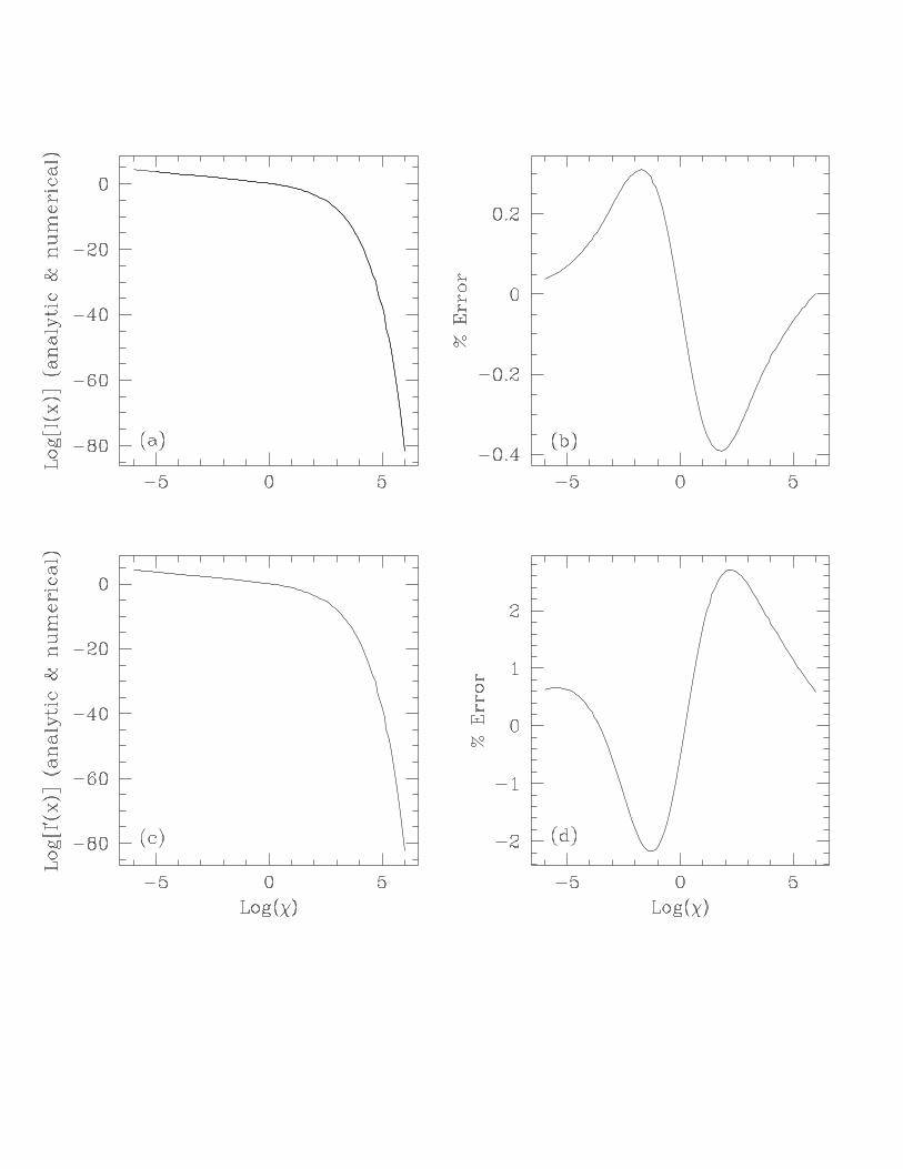
xM ≈ 63. Figures 4a, b, compare the fitting function with the exact numerical values

of I(xM) and show the residuals.

In the case of I ′(xM), we show in Appendix A. that as xM → 0

I ′(xM) → 2.1532 x−2/3M , (30)

and as xM → ∞I ′(xM) → 4.0505 x

−1/6M exp(−1.8899 x

1/3M ). (31)

Once again we combine these two limits to obtain a fitting function:

I ′(xM ) =4.0505

x1/6M

(

1 +0.40

x1/4M

+0.5316

x1/2M

)

exp(

−1.8899 x1/3M

)

. (32)

This function has a maximum error of 2.7% at xM ≈ 160. Figs. 4c, d, compare the

fitting function with the numerical values and show the residuals.

– 10 –

3.2.2. The Mildly Relativistic Regime

Using our tabulated values of ηχ as a function of β and χ, we have computed

emission spectra for isotropic thermal distributions of electrons with temperatures in

the range, 5 × 108K < T < 3.2 × 1010K. We see that at the highest temperatures the

emission is very similar to I ′(xM), equation (32), but there are significant deviations at

lower temperatures, especially at small χ. We have obtained a set of fitting functions

corresponding to each of the temperatures for which we have calculated the spectrum.

Each function is of the form

M(xM ) =4.0505α

x1/6M

(

1 +0.40β

x1/4M

+0.5316γ

x1/2M

)

exp(

−1.8896 x1/3M

)

, (33)

where α, β, γ, are all adjustable parameters which we have optimized so as to minimize

the square of the deviation of M(xM ) from the numerically calculated results. Table 1

shows the optimized parameters we obtained at the various temperatures. We expect

that as T → ∞, α, β, and γ should all → 1, since M(xM ) must approach I ′(xM).

Indeed we see that this is the case in Table 1. At lower values of T , however, the

parameters are very different from 1. This is to a large extent because the fitting

function is attempting to fit the harmonic “bumps” in the spectrum

In terms of the fitting function M(xM ), the optically thin cyclo-synchrotron

emission from a thermal plasma at temperature T is given by (cf. equation (11)),

εωdω = C R(χ, T ) dω ergs s−1 Hz−1, (34)

with

R(χ, T ) =χM(xM )

K2(1/θe), (35)

and the power is given by

ω εω = χLχ = ωb C χR(χ, T ) ergs s−1. (36)

For temperatures T > 3 × 1010 K, M(xM ) should be replaced by I ′(xM) given in

equation (32), which is equivalent to setting the fitting constants α, β, γ equal to unity.

Figs. 5, 6, show the fits at various temperatures along with the residuals, and

Table 2 shows where the maximum errors occur, both over the range log(χ) < 1 and for

log(χ) > 1. We see that the errors are particularly severe for log(χ) < 1 because of the

harmonic oscillations which are impossible to fit in detail with a simple function such

as (33). However, in many applications, the synchrotron emission will be self-absorbed,

and one would be interested primarily in log(χ) > 1. We see that the errors here are

much less severe.

We have compared our detailed numerical results with those of Petrosian (1981),

Takahara & Tsuruta (1982) and Melia (1994). We find good agreement with the former

– 11 –

two papers. The small differences in our results can be explained by the fact that they

only considered a single observer direction whereas we have averaged over all directions.

We do, however, find a serious discrepancy with Melia’s results. For instance, our

calculation shows that for T = 1010K, the spectrum peaks at log(χ) ≃ 2, whereas the

calculation by Melia indicates that the peak is at log(χ) ≃ 1 and that the emission

is insignificant at log(χ) ≃ 2. In fact, Melia’s results seem to indicate that the cutoff

frequency for the synchrotron emission is essentially independent of the temperature,

whereas it is clear from basic principles that the cutoff must increase rapidly with

increasing temperature.

4. Conclusion

The detailed calculations described in this paper bridge the gap between the

limits of nonrelativistic cyclotron emission and ultrarelativistic synchrotron emission.

We have calculated the emission due to an isotropic distribution of charged particles

moving in a magnetic field, and have shown how the spectrum changes as a function

of the particle Lorentz factor γ and the dimensionless frequency χ (defined in Eqs. 20

and 1). Figure 2 shows some results for selected cases. Included in our calculations are

all the details of the harmonic emission. This is important at low values of γ, and for

low frequencies even at high values of γ. Also, we isotropically average over observer

directions relative to the magnetic field.

Having calculated emission spectra for an array of values of γ, we have integrated

the spectra over an isotropic relativistic Maxwellian distribution of particle velocities

to calculate the spectrum of cyclo-synchrotron emission due to a thermal plasma in

a magnetic field. The results are shown in Figs. 5 and 6 for temperatures ranging

from 5 × 108 K to 3.2× 1010 K. We have obtained fitting functions M(xM ) with three

fitting constants, α, β, γ (see Eqs. 33–35 and Table 1), which provide a fairly accurate

representation of the numerical results. These fitting functions allow the spectrum to

be calculated with reasonable accuracy for any temperature > 5 × 108 K. The errors

decrease with increasing temperature in the manner indicated in Table 2.

The thermal cyclo-synchrotron spectra presented in this paper agree with most

previous results, except that our calculations are more complete since the spectra

have been integrated over all particle and observer angles. At highly relativistic

temperatures, our results agree with those given by Pacholczyk (1970), while at mildly

relativistic temperatures and for frequencies ω ≫ ωb, our results agree with those of

Petrosian (1981) and Takahara & Tsuruta (1982). There are minor deviations in the

results which can be traced to the fact that the previous authors specified a fixed

direction of the observer relative to the field rather than averaging over all directions.

– 12 –

Our results do, however, differ significantly from the calculations presented by Melia

(1994) and we have been unable to understand the reason for the discrepancy.

Finally, we note that the basic output of our calculations is a table of emission

spectra for isotropic particles of fixed velocity β or Lorentz factor γ. In this paper we

have concentrate on one application of this table, namely the calculation of thermal

cyclo-synchrotron spectra from thermal plasmas with Maxwellian velocity distributions.

The tabulated results could be convolved with any other isotropic electron distribution

function, e.g. a power law distribution, to calculate the corresponding spectrum.

Our work thus provides a “ready to use” table for determining the cyclo-synchrotron

emission from any astrophysical source with an isotropic particle and magnetic field

distribution.

Acknowledgements: This work was supported in part by NSF grants AST 9423209 (to

the Center for Astrophysics) and PHY 9407194 (to ITP, University of California, Santa

Barbara). RN thanks the ITP for hospitality.

– 13 –

A. Asymptotic Formulae for I(x) and I ′(x)

A.1. I(x)

The definition of I(x) is given in Eq. (13):

I(x) ≡ 1

x

∞∫

0

z2 exp(−z)F (x/z2)dz. (A1)

By using the approximation of F (x) given in Eq. (9), Pacholczyk (1970) showed that,

I(x) → 1

x

16π

9√3

(

x

2

)1/3

≃ 2.5593x−2/3, x ≪ 1. (A2)

In the opposite limit of x ≫ 1, we use the approximation of F (x) given in Eq. (10) to

write

I(x) →√

π

2

1

xx1/2

∞∫

0

z21

zexp[−(z + x/z2)] dz. (A3)

Employing the method of steepest descent, Petrosian (1981) showed that this integral

can be evaluated to give

I(x) → 2π

61/2exp[−(21/3 + 2−2/3) x1/3],

→ 2.5651 exp(−1.8899 x1/3), x ≫ 1. (A4)

A.2. I ′(x)

The function I ′(x) is defined by

I ′(x) =1

4π

∫

I

(

x

sin θp

)

dΩp. (A5)

We first consider the case for x ≪ 1, where we have I(x) → 2.56x−2/3. Setting

x → x/ sin θ, we obtain

I ′(x) → 2 · 2π4π

1∫

0

2.56

x2/3sin2/3 θ d(cos θ), (A6)

which can be evaluated to give

I ′(x) → 2.56

x2/3

Γ(1/2)Γ(1/3)

2 Γ(11/6), (A7)

≃ 2.153x−2/3, x ≪ 1.

– 14 –

For x ≫ 1, we have I(x) → 2.5651 exp(−1.8899x1/3), and setting x → x/ sin θ, we

obtain

I ′(x) = 2.5651

1∫

0

exp(−1.8899x1/3/ sin1/3 θ)d(cos θ). (A8)

We now use the fact that most of the emission comes from θ ≃ π/2. Setting θ = φ+π/2

we obtain

I ′(x) → 2.5651

1∫

0

exp(−1.8899x1/3/ cos1/3 φ) d(sinφ). (A9)

Setting cosφ = (1− y2)1/2, and Taylor-expanding up to y2, we finally obtain

I ′(x) → 2.5651

1∫

0

exp(−1.8899x1/3) exp(−1.8899x1/3 y2/6) dy, (A10)

=2.5651 exp(−1.8899x1/3)

2

√

π

1.8899

√

6

x1/3,

≃ 4.050471

x1/6exp(−1.8899x1/3), x ≫ 1.

Table 1: Optimal values of the parameters for different temperatures.

T (K) I ′(x)

α β γ

5× 108 0.0431 10.44 16.61

1× 109 1.121 -10.65 9.169

2× 109 1.180 -4.008 1.559

4× 109 1.045 -0.1897 0.0595

8× 109 0.9774 1.160 0.2641

1.6× 1010 0.9768 1.095 0.8332

3.2× 1010 0.9788 1.021 1.031

Table 2: List of errors and where they occur for log(χ) < 1 and for log(χ) > 1, for

different temperatures.

T (K) log(χ) < 1 % Error log(χ) > 1 % Error

log(χmax.error) log(χmax.error)

5× 108 0.1 440 2.3 85.1

1× 109 0.05 33.6 3.3 16.6

2× 109 0.0 5.9 3.0 5.3

4× 109 0.33 6.7 2.8 2.4

8× 109 0.33 5.3 1.9 0.9

1.6× 1010 0.0 7.0 1.4 0.56

3.2× 1010 0.0 7.4 1.6 0.55

References

Anderson, M. C., Keohane, J. W., Rudnick, L., 1995, ApJ, 441, 300

Bekefi, G., 1966, Radiation Processes in Plasmas (New York: John Wiley & Sons, Inc.)

Carilli, C. L., Perley, R. A., Dreher, J. W., Leahy, J. P., 1991, ApJ, 383, 554

Melia, F., 1994, ApJ, 426, 577

Meszaros, P., Laguna, P., Rees, M. J., 1993, ApJ, 415, 181

Narayan, R., Yi, I., Mahadevan, R., 1995, Nature, 374,623

Oster, L., Phys. Rev., 1960, 119, 1444

Oster, L., Phys. Rev., 1961, 121, 961

Pacholczyk, A. G., 1970, Radio Astrophysics (San Francisco: Freeman)

Paczynski, B., Rhoads, J. E., 1993, ApJ, 418, L5

Petrosian, V., 1981, ApJ, 251, 727

Rosner, H., 1958, Republic Aviation Corporation, Missile Systems Division, Technical

Report No. 206-950-3, ASTIA AD 208 852

Rybicki, G., Lightman, A., 1979, Radiative Process in Astrophysics (New York: John

Wiley & Sons, Inc.)

Schott, G. A., 1912, Electromagnetic Radiation (London: Cambridge University Press)

Schwinger, J., 1949, Phys. Rev., 75, 1912

Takahara, F., Tsuruta, S., 1982, Progress of Theoretical Physics, Vol. 67, No.2, 485

Figure Captions

Figure 1: (a) Cyclotron emission for a particle with β = 0.1. The emission is normalized

to the total emission in all harmonics. (b) Synchrotron emission for a particle with

γ = 10 from standard synchrotron theory.

Figure 2: Plots of scaled emission log(lχ) against log(χ) for (a) β = 0.2, (b) β = 0.3,

(c) β = 0.6, (d)β = 0.9, (e) γ = 5.3, (f) γ = 10.3, (g) γ = 40.3, (h)γ = 100.3. The

vertical axis is the scaled emission, lχ after the angular integrations in Eq. (22) have

been performed. lχ ≡ Lχ (c/e2 ω2

b ) = Lω (c/e2 ωb) (cf. Eq.(22)). The dashed lines show

the synchrotron limit given by Eqn. (6).

Figure 3: Polar plot of emission from a particle moving with a Lorentz factor γ = 10

at an angle of cos θp = 0.3. The magnetic field is oriented along the positive y-axis and

cos θ = 0 corresponds to the x-axis. The values of χ are (a) χ = 0.8, (b) χ = 1.4, (c)

χ = 5.0, (d) χ = 100.0.

Figure 4: (a) Plot of the analytic and numerical values for I(x) and (b) the

corresponding residuals. (c) Plot of the analytic and numerical values for I ′(x) and (d)

the corresponding residuals.

Figure 5: (a) Plots of Eqn. (34) (dashed lines) and the numerical calculation (solid

lines) for (a) T = 3.2× 1010, (b) T = 1.6× 1010, (e) T = 8× 109, (f) T = 4× 1010, and

their corresponding percentage errors (c), (d), (g), and (h).

Figure 6: (a) Plots of Eqn. (34) (dotted lines) and the numerical calculation (solid

lines) for T = 2 × 109, (b) T = 1 × 109, (e) T = 5 × 108, and their corresponding

percentage errors (c), (d), and (f).