artificial reef structures north sea
TRANSCRIPT
Artificial reef structures North Sea
Structure stability analyses in Borssele OWF and NSIL
Client:
TenneT TSO & De Rijke Noordzee
Date:
31/08/2020
Clients Reference:
Our Reference:
WP2020_1218_R1r2
Version:
Final
WP2020_1218_R1r2_Stability_eco_structures_Northsea_final.docx Page 2/50
Title
Artificial reef structures North Sea, Structure stability analyses in Borssele OWF and NSIL
Client Reference
TenneT TSO & De Rijke Noordzee WP2020_1218
Keywords
Ecological structures, North Sea, stability, scour, scour protection
Summary
The natural development of areas rich in biodiversity within the North Sea is a lengthy process. The
aim of the Rich North Sea program (Dutch: De Rijke Noordzee) is to enhance nature within offshore
windfarms by stimulating biodiversity enhancement measures. One of these measures is to place a
number of artificial reef structures on the seabed within the offshore wind farms (OWF’s) vicinity.
One of the first locations where these reefs are placed is in the North Sea Innovation Lab (also named
NSIL and Offshore Innovation Lab), off the coast of Scheveningen. Additionally, it is researched if
these reefs can also be placed in the Borssele OWF, off the coast of Zeeland, next to the Beta
substation of TenneT.
In this study the stability of the proposed structures is verified. Thereto, first the extreme MetOcean
boundary conditions (waves, flow) are identified. Next, the expected scour in the vicinity of the
structures is calculated considering the local morphological circumstances (soil composition,
bedforms, depth, etc.). Using both flow flume experiments and analytical calculations the stability of
the structures is determined, both for the failure mechanism turning over as well as sliding.
The result of the study is that scour protection should be applied, to prevent the structures from
sinking into the bed. The scour protection requirements for NSIL are higher than for Borssele OWF,
especially because the water depth at NSIL is relatively limited. Moreover, the study showed that
additional measures need to be taken to prevent the structures against turning over / sliding, as for
both locations the stability of the structures is not sufficient to be able to withstand a 1/100 year
storm. Recommendations are proposed to increase the stability, during and after installment, by e.g.
increasing the weight of the structures and making them symmetrical in shape.
Version Date Author Review & Approval
R1r0, Draft 10 – 7 – 2020 K. Koudstaal
L. van Rijn L. Perk, R. Snoek
R1r1, Final 27 – 7 – 2020 K. Koudstaal
L. van Rijn L. Perk, R. Snoek
R1r2, Final 31 – 8 – 2020 K. Koudstaal
L. van Rijn L. Perk, R. Snoek

WP2020_1218_R1r2_Stability_eco_structures_Northsea_final.docx Page 3/50
TABLE OF CONTENTS
Table of contents .................................................................................................................. 3
1 Introduction ................................................................................................................... 5
1.1 Background .......................................................................................................................... 5
1.2 Stability requirements ........................................................................................................ 5
1.3 Objective and research questions ..................................................................................... 5
1.4 Approach and chapter outline ........................................................................................... 7
2 Reference design ........................................................................................................... 8
2.1.1 Structures ......................................................................................................................................................... 8
2.1.2 Foundation ...................................................................................................................................................... 8
3 Project area, acting forces and seabed dynamics...................................................... 9
3.1 Introduction ......................................................................................................................... 9
3.2 Hydro- and Morphodynamics, at Borssele OWF ............................................................. 9
3.2.1 Introduction .................................................................................................................................................... 9
3.2.2 Water levels ................................................................................................................................................... 10
3.2.3 Wave and wind climate ............................................................................................................................ 11
3.2.4 Currents .......................................................................................................................................................... 13
3.2.5 Bed composition ......................................................................................................................................... 14
3.2.6 Local seabed mobility ............................................................................................................................... 15
3.2.7 Overview ......................................................................................................................................................... 16
3.3 Hydro- and Morphodynamics, at the Offshore Innovation Lab .................................. 18
3.3.1 Introduction .................................................................................................................................................. 18
3.3.2 Water levels ................................................................................................................................................... 18
3.3.3 Wave and wind climate ............................................................................................................................ 19
3.3.4 Currents .......................................................................................................................................................... 21
3.3.5 Bed composition ......................................................................................................................................... 22
3.3.6 Local seabed mobility ............................................................................................................................... 23
3.3.7 Overview ......................................................................................................................................................... 24
4 Scour Protection .......................................................................................................... 25
4.1 Introduction ....................................................................................................................... 25
4.2 Scour depth processes and equations ............................................................................ 25
4.3 Scour depth predictions Borssele OWF and Innovation lab plot ................................ 27
4.4 Bed protection around pile structures ........................................................................... 29
4.5 Design scour protection Reef Structure North Sea ....................................................... 32
4.5.1 Borssele OWF ............................................................................................................................................... 33
WP2020_1218_R1r2_Stability_eco_structures_Northsea_final.docx Page 4/50
4.5.2 Offshore Innovation lab ........................................................................................................................... 33
4.6 Conclusions ........................................................................................................................ 35
5 Stability ....................................................................................................................... 37
5.1 Introduction ....................................................................................................................... 37
5.2 Forces on the structure ..................................................................................................... 37
5.3 Laboratory tests ................................................................................................................ 38
5.4 Stability calculation .......................................................................................................... 40
5.4.1 Forces on the structures ........................................................................................................................... 41
5.4.2 Required resistance of the structure ................................................................................................... 42
5.5 Conclusions ........................................................................................................................ 44
6 Conclusions and recommendations for design Optimization ................................ 46
6.1 Conclusions ........................................................................................................................ 46
6.1.1 Scour protection .......................................................................................................................................... 46
6.1.2 Stability ........................................................................................................................................................... 47
6.2 Recommendations for design optimization .................................................................. 47
6.2.1 Optimization of location .......................................................................................................................... 47
6.2.2 Optimization structures and scour protection ................................................................................ 47
6.2.3 Optimization of installation methodology ....................................................................................... 48
6.2.4 General recommendations ...................................................................................................................... 49
7 References ................................................................................................................... 50
WP2020_1218_R1r2_Stability_eco_structures_Northsea_final.docx Page 5/50
1 INTRODUCTION
1.1 BACKGROUND
The natural development of areas rich in biodiversity within the North Sea is a lengthy process. The
aim of the Rich North Sea program is to enhance nature within offshore windfarms by stimulating
biodiversity enhancement measures. One of these measures is to place a number of artificial reef
structures on the seabed within the offshore wind farms (OWF’s) vicinity.
One of the first locations where these reefs are placed is in the North Sea Innovation Lab (also named
NSIL and Offshore Innovation Lab), off the coast of Scheveningen. Additionally, it is researched if
these reefs can also be placed in the Borssele OWF, off the coast of Zeeland, next to the Beta
substation of TenneT (see Figure 1.1).
Two type of reef structures are placed; one is designed to enhance the growth of blue mussels and
the other to provide a suitable location for cephalopods species to lay their eggs, see Figure 2.1. The
structures are placed on top of a layer of gravel/shell mix to provide more stability and to attract the
settlement of reef-building species like blue mussels.
The structures and the gravel/shell mix need to be resistant to the natural forces (flow, waves and
seabed dynamics) at the North Sea in these areas. The Rich North Sea asked Waterproof to provide
a proposal for a desk assessment in which an indication of the stability of the two type of structures
and the probability of outwashing of the gravel/shell mix is given for the two proposed locations. In
this document we provide our proposal for this desk assessment.
1.2 STABILITY REQUIREMENTS
The following stability requirements should be considered:
▪ Both structures should be stable enough to withstand a 100-year storm. Moving slightly within
the appointed nature enhancement area is acceptable. A minimum stability requirement is not
washing out of the appointed area within its lifetime of 40 years.
▪ The gravel/shell mix should be stable enough to withstand a 100-year storm and should not
wash out of the appointed area during its lifetime of 25 years.
▪ Both structures should be stable enough not to sink in the seabed or be covered by sandwaves.
1.3 OBJECTIVE AND RESEARCH QUESTIONS
The objective of the study is to determine the stability of the artificial reef structures and gravel/shell
layer against the forces, both related to flow/waves as well as seabed dynamics, present at two
locations (with different water depth) at the Innovation lab and within the Borssele OWF, following a
desk assessment (quickscan). The three research questions which should be answered are:
What is the probability that the three above requirements are met within the different test
parameters?
What is the minimal weight of both structures to make it stable enough to meet the
requirements and expected sand accretion of the structure?
Which additional validation steps should be executed before placement of the structures?
This report provides the answers to the formulated research questions.

WP2020_1218_R1r2_Stability_eco_structures_Northsea_final.docx Page 6/50
Figure 1.1: Location where structures are placed: Offshore innovation lab, plot 6 (upper panel) and Borssele OWF
near the Beta platform (lower panel).
Innovation lab location
OWF Borssele location

WP2020_1218_R1r2_Stability_eco_structures_Northsea_final.docx Page 7/50
1.4 APPROACH AND CHAPTER OUTLINE
The design of the structures / foundation is influenced by:
▪ The reference design of the structures / foundation
▪ Acting hydraulic forces & seabed dynamics.
▪ Boundary conditions to consider
In Figure 1.2 the approach to the study is outlined. Firstly, the reference design is regarded in chapter
2. The structures and the gravel/shell mix need to be resistant to the natural forces (flow, waves and
seabed dynamics) at the North Sea in these areas. To this end, the most important hydrodynamic
conditions and the bed composition for both areas have been determined based on the available
MetOcean and survey data, in chapter 3. Based on these conditions, the scour depth without
protection is determined with the tool SCOUR by prof. em. Leo van Rijn in chapter 4. In this chapter,
also the required scour protection layer dimensions are determined with the tool ARMOUR. The
conditions of chapter 3 also form the basis of the structure stability calculations in chapter 5. All
results are then combined in a recommendation for design optimization in chapter 6. Finally, some
final conclusions and recommendations are highlighted in chapter 7.
Figure 1.2: Study approach

WP2020_1218_R1r2_Stability_eco_structures_Northsea_final.docx Page 8/50
2 REFERENCE DESIGN
2.1.1 Structures
The reference designs for Option A and B have been provided by The Rich North Sea and are shown
in Figure 2.1. The structures are formed of individual concrete blocks with dimensions of approx. 0.5
x 0.5 m, and weigh approximately 160 kg per block (COAST, 2019). These structures are made of a
special (more porous) concrete to enhance marine growth on the structures. The structures are
formed of 2 (Type A) or 3 (Type B) vertical layers of blocks and consist of a base layer of 3 x 2 blocks
on the rock foundation and are interconnected with cables. The blocks are hollow and filled with
smaller 0.15 m cubes. Additional nature enhancement features (mussel streamers, jute / basalt cradle,
cat’s cradle) are added to make the structures an attractive habitat.
For the calculation of the stability the following aspects are of importance:
▪ Dimensions
▪ Weight of structure
▪ Drag coefficient of structure (especially incl. biofouling)
The dimensions of the structures (height, width, length) are fixed and (currently) not adjusted for
optimization of the stability. The weight of the structure can still be optimized, by increasing the
hollow space within the blocks or using concrete with different type of specific weight. The non-
optimized estimated weight of the structures is further elaborated in section 5.4, Table 5.6.The
resistance of the structures to the flow and related drag force on the structures is a very important
parameter and is depending on (1) structure dimensions in relation to flow angle and (2) biofouling.
Figure 2.1: Left panel: Type A structure, Reef Cube pyramid with mussel streamers. Right panel: Type B structure,
Reef Cube Pyramid with Cephalopod structure. Middle panel: Cut away view concrete cubes. Weight estimates are
given in section 5.4, Table 5.6.
2.1.2 Foundation
The structures are placed on a bed (foundation) consisting of a mixture of shell and gravel. The design
includes two different gradients of natural substrate (mix of empty shells and gravel).
For the calculation of the stability of the foundation the following aspects are of importance:
▪ Rock/gravel/mixture size, weight, porosity
▪ Thickness
▪ Presence of a filter layer
▪ Type of shell/gravel mixture used
The first three points are determined as a result of the scour depth analysis and required protection
calculation in chapter 3.

WP2020_1218_R1r2_Stability_eco_structures_Northsea_final.docx Page 9/50
3 PROJECT AREA, ACTING FORCES
AND SEABED DYNAMICS
3.1 INTRODUCTION
This chapter studies the hydro- and morphodynamics seen at two locations; Borssele OWF, off the
coast of Zeeland, next to the Beta substation of TenneT, and in the North Sea Innovation Lab (NSIL),
off the coast of Scheveningen. These dynamics form the boundary conditions for the scour and
stability calculations.
3.2 HYDRO- AND MORPHODYNAMICS, AT BORSSELE OWF
3.2.1 Introduction
The Borssele windfarm area is located several kilometres offshore from the coast of Zeeland, in the
southern part of the North Sea. The projected locations for the reefs in this area are next to the Beta
substation of TenneT, as shown in figure 1.
For the construction of this windfarm, an extensive MetOcean and morphodynamics study has been
performed by Deltares (2015, 2016a). For this study, the windfarm was divided into 4 different
sections and each section has been analysed individually. Additionally, several studies have been
performed to analyse the seabed for the export cables, on morphology (WaterProof, 2015) and
seabed composition (Fugro, 2016).
The hydrodynamic conditions that will be used for determining the stability of the reefs are the result
of the extensive MetOcean study from 2015, with the focus of the results in site III, as this site is most
comparable to the reef locations. The output location of this site is shown in Figure 3.1. Table 3.1
shows the coordinates and the local water depth.
Figure 3.1: OWF Borssele windfarm zone, copyright Deltares 2015

WP2020_1218_R1r2_Stability_eco_structures_Northsea_final.docx Page 10/50
Table 3.1: Coordinates location MetOcean data OWF Borssele, site III
Site Latitude Longitude Easting
[m, UTM 31N]
Northing
[m, UTM 31N]
Depth
[m +MSL]
Site III 2.96111 N 51.694424 E 497312 5727053 -35.1
3.2.2 Water levels
Based on the MetOcean data, the following can be said about the local extreme water levels (see
also Table 3.2 and Table 3.3):
▪ The highest astronomical tide (HAT) is of 2.10m (relative to MSL) and the lowest astronomical
tide (LAT) is -1.55m (relative to MSL).
▪ The 100-year return value of the extreme high total water level is 3.20m and of the extreme low
water level is -2.25m.
Table 3.2: Tidal characteristics at the OWF Borssele windfarm, site III.
Tide level Relative to MSL [m] Relative to LAT [m]
HAT 2.05 3.65
MHWS 1.55 3.20
MHWN 0.90 2.50
MSL 0.00 1.60
MLWN -0.90 0.70
MLWS -1.25 0.35
LAT -1.60 0.00
Table 3.3: Extreme high and low water levels (HWL and LWL) at the OWF Borssele windfarm, site III, for several
return periods.
Return period [years]
Extreme high water
levels, relative to MSL
[m]
Extreme low water
levels, relative to MSL
[m]
1 2.40 (2.35 - 2.45) -1.80 (-1.85 - -1.80)
2 2.50 (2.45 - 2.60) -1.90 (-1.95 - -1.85)
5 2.70 (2.55 - 2.80) -1.95 (-2.05 - -1.90)
10 2.80 (2.65 - 3.00) -2.05 (-2.15 - -1.95)
50 3.10 (2.75 - 3.50) -2.20 (-2.50 - -2.00)
100 3.20 (2.80 - 3.80) -2.25 (-2.65 - -2.05)
WP2020_1218_R1r2_Stability_eco_structures_Northsea_final.docx Page 11/50
3.2.3 Wave and wind climate
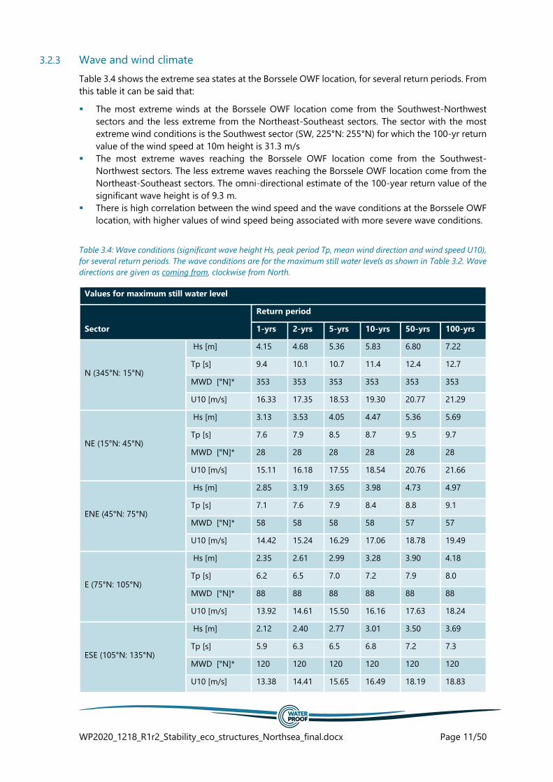
Table 3.4 shows the extreme sea states at the Borssele OWF location, for several return periods. From
this table it can be said that:
▪ The most extreme winds at the Borssele OWF location come from the Southwest-Northwest
sectors and the less extreme from the Northeast-Southeast sectors. The sector with the most
extreme wind conditions is the Southwest sector (SW, 225°N: 255°N) for which the 100-yr return
value of the wind speed at 10m height is 31.3 m/s
▪ The most extreme waves reaching the Borssele OWF location come from the Southwest-
Northwest sectors. The less extreme waves reaching the Borssele OWF location come from the
Northeast-Southeast sectors. The omni-directional estimate of the 100-year return value of the
significant wave height is of 9.3 m.
▪ There is high correlation between the wind speed and the wave conditions at the Borssele OWF
location, with higher values of wind speed being associated with more severe wave conditions.
Table 3.4: Wave conditions (significant wave height Hs, peak period Tp, mean wind direction and wind speed U10),
for several return periods. The wave conditions are for the maximum still water levels as shown in Table 3.2. Wave
directions are given as coming from, clockwise from North.
Values for maximum still water level
Sector
Return period
1-yrs 2-yrs 5-yrs 10-yrs 50-yrs 100-yrs
N (345°N: 15°N)
Hs [m] 4.15 4.68 5.36 5.83 6.80 7.22
Tp [s] 9.4 10.1 10.7 11.4 12.4 12.7
MWD [°N]* 353 353 353 353 353 353
U10 [m/s] 16.33 17.35 18.53 19.30 20.77 21.29
NE (15°N: 45°N)
Hs [m] 3.13 3.53 4.05 4.47 5.36 5.69
Tp [s] 7.6 7.9 8.5 8.7 9.5 9.7
MWD [°N]* 28 28 28 28 28 28
U10 [m/s] 15.11 16.18 17.55 18.54 20.76 21.66
ENE (45°N: 75°N)
Hs [m] 2.85 3.19 3.65 3.98 4.73 4.97
Tp [s] 7.1 7.6 7.9 8.4 8.8 9.1
MWD [°N]* 58 58 58 58 57 57
U10 [m/s] 14.42 15.24 16.29 17.06 18.78 19.49
E (75°N: 105°N)
Hs [m] 2.35 2.61 2.99 3.28 3.90 4.18
Tp [s] 6.2 6.5 7.0 7.2 7.9 8.0
MWD [°N]* 88 88 88 88 88 88
U10 [m/s] 13.92 14.61 15.50 16.16 17.63 18.24
ESE (105°N: 135°N)
Hs [m] 2.12 2.40 2.77 3.01 3.50 3.69
Tp [s] 5.9 6.3 6.5 6.8 7.2 7.3
MWD [°N]* 120 120 120 120 120 120
U10 [m/s] 13.38 14.41 15.65 16.49 18.19 18.83

WP2020_1218_R1r2_Stability_eco_structures_Northsea_final.docx Page 12/50
Values for maximum still water level
Sector
Return period
1-yrs 2-yrs 5-yrs 10-yrs 50-yrs 100-yrs
SE (135°N: 165°N)
Hs [m] 2.45 2.73 3.18 3.51 4.19 4.50
Tp [s] 6.1 6.4 6.9 7.1 7.8 8.0
MWD [°N]* 151 151 151 151 151 151
U10 [m/s] 15.17 16.10 17.32 18.23 20.28 21.15
S (165°N: 195°N)
Hs [m] 3.73 3.98 4.37 4.62 5.18 5.37
Tp [s] 7.2 7.5 7.8 8.0 8.5 8.6
MWD [°N]* 186 189 189 189 190 190
U10 [m/s] 19.52 20.60 22.01 23.06 25.45 26.46
SSW (195°N: 225°N)
Hs [m] 4.90 5.28 5.78 6.10 6.83 7.07
Tp [s] 8.5 8.7 9.1 9.4 9.9 10.1
MWD [°N]* 214 215 215 216 216 216
U10 [m/s] 21.61 22.93 24.65 25.93 28.81 30.03
SW (225°N: 255°N)
Hs [m] 5.22 5.54 6.15 6.57 7.50 7.87
Tp [s] 8.8 8.9 9.5 9.7 10.5 10.7
MWD [°N]* 238 240 240 241 241 241
U10 [m/s] 21.83 23.25 25.13 26.55 29.87 31.30
W (255°N: 285°N)
Hs [m] 4.95 5.35 6.09 6.55 7.59 8.03
Tp [s] 8.7 9.1 9.6 10.1 10.7 11.3
MWD [°N]* 269 270 270 270 270 270
U10 [m/s] 20.13 21.56 23.30 24.53 27.09 28.09
NNW (285°N: 315°N)
Hs [m] 4.89 5.20 5.67 6.03 6.83 7.09
Tp [s] 9.1 9.4 9.7 10.2 10.5 10.6
MWD [°N]* 300 301 301 301 301 301
U10 [m/s] 19.15 20.05 21.30 22.27 24.68 25.78
NW (315°N: 345°N)
Hs [m] 4.82 5.37 6.14 6.69 7.90 8.45
Tp [s] 9.9 10.4 11.2 11.5 12.5 12.8
MWD [°N]* 331 331 331 331 331 331
U10 [m/s] 17.56 18.71 20.18 21.24 23.57 24.51
OMNI
Hs [m] 6.03 6.52 7.21 7.70 8.83 9.26
Tp [s] 9.8 10.3 10.6 11.2 12.0 12.4
MWD [°N]* - - - - - -
U10 [m/s] 22.83 24.10 25.78 27.05 30.02 31.30

WP2020_1218_R1r2_Stability_eco_structures_Northsea_final.docx Page 13/50
3.2.4 Currents
The extreme currents are based on the combined effect of tidal currents and wind. It can be said that
(see Table 3.5):
▪ The most dominant flow directions are in North-Northeast and South-Southwest direction
(going to), due to the dominance of the tidal currents.
▪ The 100-year return value estimates of the depth-averaged current for the main directional
sectors North-Northeast and South-Southwest at the Borssele OWF location are 1.2m/s
respectively 1.0m/s.
Table 3.5: Current profile for the NNE sector (including wind effects) for several return periods. Currents are defined
as going towards direction, clockwise from North.
Sector NNE Return Period
Depth
% total depth
1-yrs
[m/s]
2-yrs
[m/s]
5-yrs
[m/s]
10-yrs
[m/s]
50-yrs
[m/s]
100-yrs
[m/s]
100 1.40 1.45 1.51 1.56 1.66 1.71
90 1.36 1.40 1.46 1.51 1.61 1.66
80 1.31 1.36 1.41 1.46 1.56 1.60
70 1.27 1.31 1.36 1.40 1.50 1.54
60 1.22 1.26 1.31 1.35 1.44 1.48
50 1.17 1.20 1.25 1.29 1.37 1.41
40 1.11 1.14 1.19 1.22 1.30 1.33
30 1.05 1.08 1.12 1.15 1.22 1.25
20 0.97 0.99 1.03 1.06 1.12 1.15
10 0.85 0.88 0.91 0.93 0.99 1.01
5 0.76 0.78 0.81 0.83 0.88 0.90
Table 3.6: Current profile for the SSW sector (including wind effects) for several return periods. Currents are defined
as going towards direction, clockwise from North.
Sector SSW Return Period
Depth % total
depth
1-yrs
[m/s]
2-yrs
[m/s]
5-yrs
[m/s]
10-yrs
[m/s]
50-yrs
[m/s]
100-yrs
[m/s]
100 1.42 1.45 1.49 1.52 1.59 1.62
90 1.37 1.40 1.43 1.46 1.53 1.55
80 1.31 1.34 1.38 1.40 1.46 1.49
70 1.26 1.28 1.32 1.34 1.40 1.42
60 1.20 1.23 1.25 1.28 1.33 1.35
50 1.14 1.16 1.19 1.21 1.25 1.27

WP2020_1218_R1r2_Stability_eco_structures_Northsea_final.docx Page 14/50
Sector SSW Return Period
Depth % total
depth
1-yrs
[m/s]
2-yrs
[m/s]
5-yrs
[m/s]
10-yrs
[m/s]
50-yrs
[m/s]
100-yrs
[m/s]
40 1.08 1.10 1.12 1.14 1.17 1.19
30 1.00 1.02 1.04 1.05 1.09 1.10
20 0.92 0.93 0.95 0.96 0.99 1.00
10 0.80 0.81 0.83 0.83 0.86 0.86
5 0.71 0.72 0.73 0.74 0.75 0.76
3.2.5 Bed composition
Based on the surveys along the OWF Borssele cable trajectory, and core data from the DINOLoket, it
can be said that (see Figure 3.2):
▪ The bed is composed of sandy materials;
There is almost no silt material present at the surface
Deeper layers are composed of very dense silty sand
▪ The average grainsize, D50, is in the order of 400 μm

WP2020_1218_R1r2_Stability_eco_structures_Northsea_final.docx Page 15/50
Figure 3.2: Bed composition based on core data of the DINOLoket
3.2.6 Local seabed mobility
The local depth at the OWF Borssele Beta platform is rather deep, as shown in Figure 3.3. The
overlapping area between NID and UXO survey area varies between 28 and 31 m depth (LAT) or 29.5
– 32.5 m MSL.
In this area, three forms of seabed dynamics are of importance:
▪ Sandwaves: the projected location lies in the middle of a sandwave field. One sandwave is of
importance; located just on the border of the NID area (see Figure 3.3 and Figure 3.4). This

WP2020_1218_R1r2_Stability_eco_structures_Northsea_final.docx Page 16/50
sandwave is several meters high compared to the average surrounding bed and has a migration
rate of on average 0.6 m/y (WaterProof, 2017 & Deltares, 2015) in NE -NNE direction.
▪ Megaripples: Megaripples in the Borssele wind farm zone have typical wavelengths of 8 to 15m.
On average in the vicinity of the Borssele OWF location, the megaripple height equals 0.7 m
(Deltares 2015). An example of these ripples, on top of the sandwaves, can be seen in Figure 3.4.
▪ Man-made interference: in the latest survey the burial of the cables and the installation of the
beta platform can be seen.
Figure 3.3: Bathymetric overview of the projected location at the OWF Borssele Beta Platform. (Left panel): OWF
Borssele cable route, towards to the projected location. (Right panel): Zoom of projected location, which is bounded
by the UXO survey area (black box) and the NID area (green).
Figure 3.4: Sandwave at the red line of Figure 3.3, as seen from South to North for 3 different surveys.
3.2.7 Overview
Below an overview is given of the most important hydrodynamic and morphological findings.
▪ Most severe currents at the Borssele OWF location come from the North-Northeast and South-
Southwest sectors; The 100-year return value estimates of the depth-averaged current for these
directional sectors are 1.2m/s and 1.0m/s respectively;
WP2020_1218_R1r2_Stability_eco_structures_Northsea_final.docx Page 17/50
▪ The most extreme winds at the Borssele OWF location come from the Southwest-Northwest
sectors and the less extreme from the Northeast-Southeast sectors. The sector with the most
extreme wind conditions is the Southwest sector (SW, 225°N: 255°N) for which the 100-yr return
value of the wind speed at 10m height is 31.3 m/s;
▪ The most extreme waves reaching the Borssele OWF location come from the Southwest-
Northwest sectors. The less extreme waves reaching the Borssele OWF location come from the
Northeast-Southeast sectors. The omni-directional estimate of the 100-year return value of the
significant wave height is of 9.3 m;
▪ The bed is composed of sandy materials;
There is almost no silt material present at the surface;
Deeper layers are composed of very dense silty sand;
▪ The average grainsize, D50, is in the order of 400 μm.
▪ Sandwaves are the main cause of local steeper slopes in the area. One big and one smaller
sandwave are present at the projected location of the structures. These sandwaves move in NE
– NNE direction with on average a migration speed of 0.6 m/y
▪ Megaripples are present on top of the sandwaves, with an average height of 0.7 m and an
average length of 8 – 15 m.

WP2020_1218_R1r2_Stability_eco_structures_Northsea_final.docx Page 18/50
3.3 HYDRO- AND MORPHODYNAMICS, AT THE OFFSHORE INNOVATION LAB
3.3.1 Introduction
The HKZ windfarm area is located several kilometres offshore from the coast of Holland, in the
southern part of the North Sea. The projected location for the reef in this area are next to the export
cables towards the HKZ windfarm, around KP 20-25, just north of disposal site Loswal North-West,
as shown in Figure 1.1. Plot 6 will become available for the structures.
For the construction of the HKZ windfarm and cable trajectories, an extensive MetOcean and study
has been performed by DHI (2017) and Svasek (2016). Only the MetOcean study by DHI has
determined the conditions for the different return periods. The output location for the study is
confined to only 1 location, i.e. the most conservative location, at the northwest corner of the
windfarm area (Figure 1.1).
Additionally, several studies have been performed to analyse the seabed for the export cables, on
morphology (WaterProof, 2017) and seabed composition (Fugro, 2017).
The hydrodynamic conditions that will be used for determining the stability of the reefs are the result
of the extensive MetOcean study from 2017. The output location of this site is shown in Figure 3.5.
Table 3.7 shows the coordinates and the local water depth.
Table 3.7: Coordinates location MetOcean data HKZ
Easting [m, UTM 31N] Northing [m, UTM 31N] Depth [m +MSL] Depth [m +LAT]
566838 5803980 -27.96 -27.05
Figure 3.5: HKZ windfarm zone, copyright DHI 2017. The output location of the MetOcean study is indicated by
the purple square.
3.3.2 Water levels
Based on the MetOcean data, the following can be said about the local extreme water levels (see
also Table 3.8 and Table 3.9):
▪ The highest astronomical tide (HAT) is of 1.07m (relative to MLS) and the lowest astronomical
tide (LAT) is -0.91m (relative to MSL).

WP2020_1218_R1r2_Stability_eco_structures_Northsea_final.docx Page 19/50
▪ The 100-year return value of the extreme high total water level is 3.20m and of the extreme low
water level is -2.1m.
Table 3.8: Tidal characteristics at the HKZ windfarm.
Tide level Relative to MSL [m] Relative to LAT [m]
HAT 1.07 1.98
MHWS 0.87 1.78
MHWN 0.56 1.47
MSL 0 0.91
MLWN -0.44 0.47
MLWS -0.66 0.25
LAT -0.91 0
Table 3.9: Extreme high and low water levels (HWL and LWL) at the HKZ windfarm, for several return periods.
Return period [years]
Extreme high water
levels, relative to MSL
[m]
Extreme low water
levels, relative to MSL
[m]
1 2.10 -1.30
2 2.20 -1.40
5 2.50 -1.60
10 2.60 -1.70
50 3.10 -2.00
100 3.20 -2.10
3.3.3 Wave and wind climate
Table 3.10 shows the extreme sea states at the HKZ windfarm, for several return periods. From this
table it can be said that:
▪ The most extreme winds at the HKZ windfarm come from the Southwest-Northwest sectors and
the less extreme from the Northeast-Southeast sectors. The sector with the most extreme wind
conditions is the Southwest sector (SW, 225°N: 255°N) for which the 100-yr return value of the
wind speed at 10m height is 32.0 m/s
▪ More than 50% of the time, waves come from between N and NW with the more extreme waves
coming from NNW. The south westerly sector also contains more than 20% of the waves.
▪ The most extreme waves reaching the HKZ windfarm come from the Southwest-Northwest
sectors. The less extreme waves reaching the HKZ windfarm come from the Northeast-Southeast
sectors. The omni-directional estimate of the 100-year return value of the significant wave height
is of 7.2 m.
▪ There is high correlation between the wind speed and the wave conditions at the HKZ windfarm
location, with higher values of wind speed being associated with more severe wave conditions.

WP2020_1218_R1r2_Stability_eco_structures_Northsea_final.docx Page 20/50
Table 3.10: Wave conditions (significant wave height Hs, peak period Tp, mean wind direction and wind speed
U10), for several return periods. The wave conditions are for the maximum still water levels as shown in Table 8.
Wave directions are given as coming from, clockwise from North.
Values for maximum still water level
Sector
Return period
1-yrs 2-yrs 5-yrs 10-yrs 50-yrs 100-yrs
N (345°N: 15°N)
Hs [m] 5.60 5.90 6.30 6.60 7.10 7.30
Tp [s] 12.8 13.3 14.0 14.5 15.3 15.7
U10 [m/s] 23.27 24.84 26.61 27.84 30.47 31.53
NE (15°N: 45°N)
Hs [m] 3.50 3.70 4.00 4.20 4.60 4.80
Tp [s] 7.8 8.1 8.4 8.6 9.1 9.3
U10 [m/s] 22.10 22.83 23.77 24.45 25.97 26.60
ENE (45°N: 75°N)
Hs [m] 3.50 3.70 4.00 4.20 4.60 4.80
Tp [s] 7.1 7.3 7.6 7.8 8.1 8.3
U10 [m/s] 22.10 22.83 23.77 24.45 25.97 26.60
E (75°N: 105°N)
Hs [m] 3.50 3.70 4.00 4.20 4.60 4.80
Tp [s] 6.8 7.0 7.2 7.4 7.7 7.8
U10 [m/s] 22.10 22.83 23.77 24.45 25.97 26.60
ESE (105°N: 135°N)
Hs [m] 3.50 3.70 4.00 4.20 4.60 4.80
Tp [s] 6.8 7.0 7.2 7.4 7.7 7.8
U10 [m/s] 22.10 22.83 23.77 24.45 25.97 26.60
SE (135°N: 165°N)
Hs [m] 3.50 3.70 4.00 4.20 4.60 4.80
Tp [s] 6.7 6.8 7.1 7.2 7.5 7.7
U10 [m/s] 22.10 22.83 23.77 24.45 25.97 26.60
S (165°N: 195°N)
Hs [m] 3.50 3.70 4.00 4.20 4.60 4.80
Tp [s] 7.0 7.2 7.5 7.6 8.0 8.1
U10 [m/s] 23.88 25.62 27.37 28.54 31.03 32.03
SSW (195°N: 225°N)
Hs [m] 5.10 5.40 5.80 6.10 6.60 6.90
Tp [s] 9.3 9.6 10.0 10.2 10.7 10.9
U10 [m/s] 23.88 25.62 27.37 28.54 31.03 32.03
SW (225°N: 255°N) Hs [m] 5.10 5.40 5.80 6.10 6.60 6.90
Tp [s] 9.8 10.0 10.4 10.7 11.1 11.4

WP2020_1218_R1r2_Stability_eco_structures_Northsea_final.docx Page 21/50
Values for maximum still water level
Sector
Return period
1-yrs 2-yrs 5-yrs 10-yrs 50-yrs 100-yrs
U10 [m/s] 23.88 25.62 27.37 28.54 31.03 32.03
W (255°N: 285°N)
Hs [m] 5.10 5.40 5.80 6.10 6.60 6.90
Tp [s] 9.3 9.5 9.9 10.1 10.6 10.8
U10 [m/s] 23.88 25.62 27.37 28.54 31.03 32.03
NNW (285°N: 315°N)
Hs [m] 5.60 5.90 6.30 6.60 7.10 7.30
Tp [s] 10.5 10.9 11.3 11.6 12.1 12.3
U10 [m/s] 23.27 24.84 26.61 27.84 30.47 31.53
NW (315°N: 345°N)
Hs [m] 5.60 5.90 6.30 6.60 7.10 7.30
Tp [s] 11.6 12.1 12.6 13.1 13.8 14.0
U10 [m/s] 23.27 24.84 26.61 27.84 30.47 31.53
OMNI
Hs [m] 5.40 5.70 6.20 6.40 7.00 7.20
Tp [s] 10.6 11.0 11.5 11.8 12.4 12.6
U10 [m/s] 24.33 25.05 27.02 28.26 30.82 31.84
3.3.4 Currents
The extreme currents are based on the combined effect of tidal currents and wind. Based on Table
3.11 it can be said that:
▪ The most dominant flow directions are in North-Northeast and South-Southwest direction
(going to), due to the dominance of the tidal currents.
▪ The 100-year return value estimates of the depth-averaged current for the main directional
sectors North-Northeast and South-Southwest at the Borssele OWF location are 1.05m/s
respectively 0.85m/s.
Table 3.11: Current profile for the NNE sector (including wind effects) for several return periods. Currents are
defined as going towards direction, clockwise from North.
Sector NNE Return Period
Depth
% total depth
1-yrs
[m/s]
2-yrs
[m/s]
5-yrs
[m/s]
10-yrs
[m/s]
50-yrs
[m/s]
100-yrs
[m/s]
100 1.28 1.34 1.41 1.47 1.59 1.64
5 0.68 0.69 0.70 0.71 0.73 0.74
Depth-
integrated (~33) 0.93 0.95 0.98 1.00 1.04 1.06

WP2020_1218_R1r2_Stability_eco_structures_Northsea_final.docx Page 22/50
Table 3.12: Current profile for the SSW sector (including wind effects) for several return periods. Currents are
defined as going towards direction, clockwise from North.
Sector SSW Return Period
Depth % total
depth
1-yrs
[m/s]
2-yrs
[m/s]
5-yrs
[m/s]
10-yrs
[m/s]
50-yrs
[m/s]
100-yrs
[m/s]
100 0.99 1.02 1.06 1.09 1.15 1.18
5 0.55 0.55 0.56 0.57 0.58 0.59
Depth-
integrated (~33) 0.75 0.77 0.78 0.80 0.82 0.84
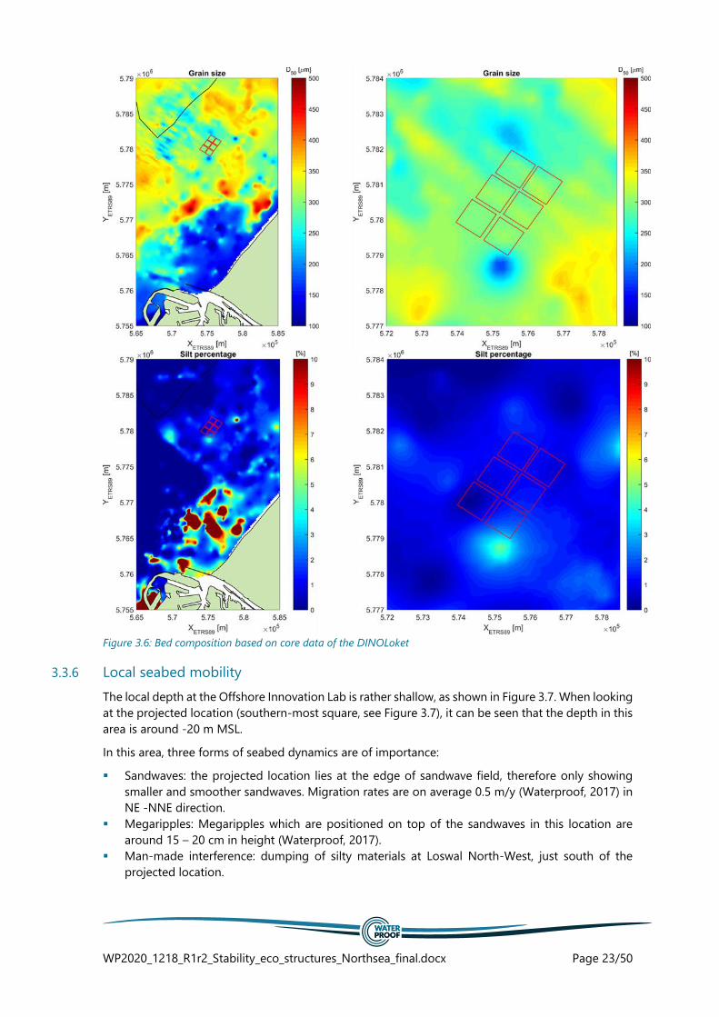
3.3.5 Bed composition
Based on the surveys along the HKZ cable trajectory, and core data from the DINOLoket (Figure 3.6),
it can be said that:
▪ The bed is mostly composed of fine to medium sandy materials;
Near the disposal site Loswal North-West there is some silt present in the surface
material
Deeper layers are mostly composed medium sand; occasionally a layer slightly silty
sand is present
▪ The average grainsize, D50, is in the order of 250-350 μm
WP2020_1218_R1r2_Stability_eco_structures_Northsea_final.docx Page 23/50
Figure 3.6: Bed composition based on core data of the DINOLoket
3.3.6 Local seabed mobility
The local depth at the Offshore Innovation Lab is rather shallow, as shown in Figure 3.7. When looking
at the projected location (southern-most square, see Figure 3.7), it can be seen that the depth in this
area is around -20 m MSL.
In this area, three forms of seabed dynamics are of importance:
▪ Sandwaves: the projected location lies at the edge of sandwave field, therefore only showing
smaller and smoother sandwaves. Migration rates are on average 0.5 m/y (Waterproof, 2017) in
NE -NNE direction.
▪ Megaripples: Megaripples which are positioned on top of the sandwaves in this location are
around 15 – 20 cm in height (Waterproof, 2017).
▪ Man-made interference: dumping of silty materials at Loswal North-West, just south of the
projected location.

WP2020_1218_R1r2_Stability_eco_structures_Northsea_final.docx Page 24/50
Figure 3.7: Bathymetric overview of the projected location at the Offshore innovation lab. (Left panel): HKZ cable
route, next to the projected location. (Right panel): Zoom of projected location, where the southern-most square
will be used for the Offshore Innovation Lab.
3.3.7 Overview
Below an overview is given of the most important hydrodynamic and morphological findings.
▪ Most severe currents at the HKZ windfarm come from the North-Northeast and South-Southwest
sectors; The 100-year return value estimates of the depth-averaged current for these directional
sectors are 1.05m/s and 0.85m/s respectively;
▪ The most extreme winds at the HKZ windfarm come from the Southwest-Northwest sectors and
the less extreme from the Northeast-Southeast sectors. The sector with the most extreme wind
conditions is the Southwest sector (SW, 225°N: 255°N) for which the 100-yr return value of the
wind speed at 10m height is 32 m/s;
▪ The most extreme waves reaching the HKZ windfarm come from the Southwest-Northwest
sectors. The less extreme waves reaching the HKZ windfarm come from the Northeast-Southeast
sectors. The omni-directional estimate of the 100-year return value of the significant wave height
is of 7.2 m;
▪ The bed is composed of sandy materials;
There is almost no silt material present at the surface;
Deeper layers are composed of very dense silty sand;
▪ The average grainsize, D50, is in the order of 250-350 μm.
▪ The sandwaves in this area are mild in both height and slope, as the location is on the very
eastern edge of the sand wave field. These small sandwaves move in NE – NNE direction with on
average a migration speed of 0.8 m/y and do not show the sharp crests as at the HKZ windfarm
area.
▪ Megaripples are present on top of the sandwaves, with an average height of 0.15 – 0.20 m
▪ Disposal site Loswal North West is located closely to the projected location. This disposal site is
mainly used for silty sediments.
WP2020_1218_R1r2_Stability_eco_structures_Northsea_final.docx Page 25/50
4 SCOUR PROTECTION
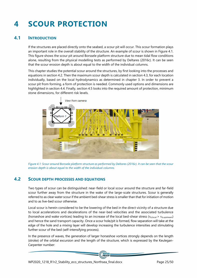
4.1 INTRODUCTION
If the structures are placed directly onto the seabed, a scour pit will occur. This scour formation plays
an important role in the overall stability of the structure. An example of scour is shown in Figure 4.1.
This figure shows the scour pit around Borssele platform structure due to mean tidal flow conditions
alone, resulting from the physical modelling tests as performed by Deltares (2016c). It can be seen
that the scour erosion depth is about equal to the width of the individual columns.
This chapter studies the potential scour around the structures, by first looking into the processes and
equations in section 4.2. Then the maximum scour depth is calculated in section 4.3, for each location
individually, based on the local hydrodynamics as determined in chapter 3. In order to prevent a
scour pit from forming, a form of protection is needed. Commonly used options and dimensions are
highlighted in section 4.4. Finally, section 4.5 looks into the required amount of protection, minimum
stone dimensions, for different risk levels.
Figure 4.1: Scour around Borssele platform structure as performed by Deltares (2016c). It can be seen that the scour
erosion depth is about equal to the width of the individual columns.
4.2 SCOUR DEPTH PROCESSES AND EQUATIONS
Two types of scour can be distinguished: near-field or local scour around the structure and far-field
scour further away from the structure in the wake of the large-scale structures. Scour is generally
referred to as clear water scour if the ambient bed-shear stress is smaller than that for initiation of motion
and to as live-bed scour otherwise.
Local scour is herein considered to be the lowering of the bed in the direct vicinity of a structure due
to local accelerations and decelerations of the near-bed velocities and the associated turbulence
(horseshoe and wake vortices) leading to an increase of the local bed-shear stress (b,local > b,upstream)
and hence the sand transport capacity. Once a scour hole/pit is formed, flow separation will take at the
edge of the hole and a mixing layer will develop increasing the turbulence intensities and stimulating
further scour of the bed (self-intensifying process).
In the presence of waves, the generation of larger horseshoe vortices strongly depends on the length
(stroke) of the orbital excursion and the length of the structure, which is expressed by the Keulegan-
Carpenter number:

WP2020_1218_R1r2_Stability_eco_structures_Northsea_final.docx Page 26/50
KC=UwT/Ls with,
Uw= peak orbital velocity,
T= wave period
Ls= length of structure normal to waves.
Horseshoe vortices cannot really develop for KC< 5 (small waves). Therefore, relative scour (scour
depth /structure length) is less for larger structures. As the diameter D of round structures increases,
the strength of the vortices weakens and for very large round structures the vortex motions have
little effect on the scouring process. The relative scour depth for small diameter (slender) structures
in water depth h with D/h < 0.3 is about 1D, whereas the scour depth for large diameter structures
with D/h 2 is about 0.35 D (Whitehouse et al., 2012). Using h=10 m; Dsmall=5 m and Dlarge=20 m,
the absolute scour depth is about 5 m for a small diameter structure and about 0.35x20=7 m for a
large diameter structure.
The scour develops in time to an equilibrium depth and length. Scour will gradually cease when (i)
the local bed shear (b) in the deepest part of the scour hole/pit is below the critical stress (b,cr) for
initiation of motion of sand particles or ii) when the supply of sand from upstream is equal to the
local transport of sand (b,local b,upstream).
Figure 4.2: Flow around a pile. From left to right, top to bottom: (1) vortices structure; (2) amplification; (3)
velocities. Van Eijk (2016)
An impression of the amplification (=(b,local/b,upstream) of the bed-shear stress around a structure in
comparison with the bed-shear stress in undisturbed conditions upstream of the structure can be
obtained from measurements and numerical modelling. Hjorth (1975) published amplification factor
results for 8 experimental runs at small scale laboratory conditions with pile diameter of D = 0.05
and 0.075m, water depth of h = 0.1 and 0.2m; flow velocity of U = 0.15 and 0.30 m/s. Figure 4.2 right
shows measured amplification factors and computed factors based on numerical CDF-model for an
experiment of Hjorth (1975) with U=0.3 m/s, h=0.1 m and D=0.05 m. Measured amplification factors
WP2020_1218_R1r2_Stability_eco_structures_Northsea_final.docx Page 27/50
are rather high (up to 10) compared to those (up to 4) produced by the numerical model. The zone
influenced by the structure extends to about 0.5 D on both sides of the structure and about 3D on
the downstream side.
Scour is enhanced by wave stirring and wave reflection in the case of large-scale structures and by
breaking/plunging waves in shallow water. Excessive scour close to the structure may ultimately lead
to instability/failure of the structure.
A dramatic example of failure due to scouring processes is the sinking of submerged coastal
structures on the sandy seabed (0.25 mm sand) in the breaker zone at Santa Maria del Mar (SMM)
Beach in Southwest Spain (Munoz-Peres et al. 2015) in mesotidal conditions (neap-spring range of
1.20 to 3.80 m). The structure consisted of precast modular concrete elements placed at a depth of
about 2.5 m without scour protection. The sinking of the concrete modules in a near-shore sandy
seafloor started immediately after placement and ended 3 weeks later when the modules reached
the rocky sub-bottom. The total sinking was of the order of 1.2 to 1.5 m. Big scour pits with cross-
shore length scales of 15 m were present on both sides of the structure.
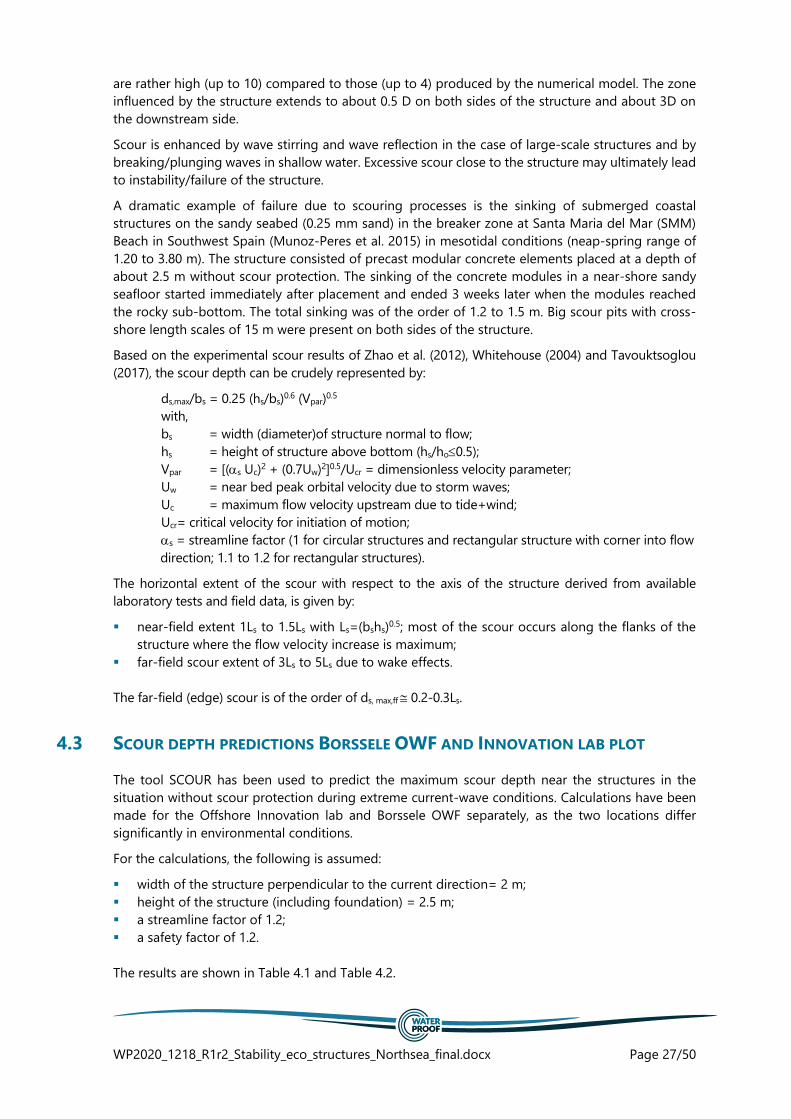
Based on the experimental scour results of Zhao et al. (2012), Whitehouse (2004) and Tavouktsoglou
(2017), the scour depth can be crudely represented by:
ds,max/bs = 0.25 (hs/bs)0.6 (Vpar)0.5
with,
bs = width (diameter)of structure normal to flow;
hs = height of structure above bottom (hs/ho0.5);
Vpar = [(s Uc)2 + (0.7Uw)2]0.5/Ucr = dimensionless velocity parameter;
Uw = near bed peak orbital velocity due to storm waves;
Uc = maximum flow velocity upstream due to tide+wind;
Ucr= critical velocity for initiation of motion;
s = streamline factor (1 for circular structures and rectangular structure with corner into flow
direction; 1.1 to 1.2 for rectangular structures).
The horizontal extent of the scour with respect to the axis of the structure derived from available
laboratory tests and field data, is given by:
▪ near-field extent 1Ls to 1.5Ls with Ls=(bshs)0.5; most of the scour occurs along the flanks of the
structure where the flow velocity increase is maximum;
▪ far-field scour extent of 3Ls to 5Ls due to wake effects.
The far-field (edge) scour is of the order of ds, max,ff 0.2-0.3Ls.
4.3 SCOUR DEPTH PREDICTIONS BORSSELE OWF AND INNOVATION LAB PLOT
The tool SCOUR has been used to predict the maximum scour depth near the structures in the
situation without scour protection during extreme current-wave conditions. Calculations have been
made for the Offshore Innovation lab and Borssele OWF separately, as the two locations differ
significantly in environmental conditions.
For the calculations, the following is assumed:
▪ width of the structure perpendicular to the current direction= 2 m;
▪ height of the structure (including foundation) = 2.5 m;
▪ a streamline factor of 1.2;
▪ a safety factor of 1.2.
The results are shown in Table 4.1 and Table 4.2.

WP2020_1218_R1r2_Stability_eco_structures_Northsea_final.docx Page 28/50
Table 4.1: Predicted scour depths; Borssele OWF
Return
period
[years]
Water
depth
[m]
High and
Low Water
to MSL
[m]
Depth-averaged
current velocity
flood to NE and
ebb to SW
[m/s]
Significant
wave
height
[m] and
wave
period [s]
Sediment
size d50;
d90
[mm]
Maximum
scour
depth
[m]
1 31 2.4 -1.8 1.1 1.08 5.22; 8.8 0.4; 1 1.40
5 31 2.7 -1.95 1.19 1.12 6.15; 9.5 0.4; 1 1.50
10 31 2.8 -2.05 1.22 1.14 6.57; 9.7 0.4; 1 1.55
50 31 3.1 -2.2 1.30 1.17 7.50; 10.5 0.4; 1 1.60
100 31 3.2 -2.25 1.33 1.19 7.87; 10.7 0.4; 1 1.65
Table 4.2: Predicted scour depths; Offshore Innovation Lab
Return
period
[years]
Water
depth
[m]
High and
Low Water
to MSL
[m]
Depth-averaged
current velocity
flood to NE and
ebb to SW
[m/s]
Significant
wave
height
[m] and
wave
period [s]
Sediment
size d50;
d90
[mm]
Maximum
scour
depth
[m]
1 20 2.1 -1.3 0.93 0.75 5.6; 12.8 0.3; 1 1.65
5 20 2.5 -1.6 0.98 0.78 6.3; 14.0 0.3; 1 1.7
10 20 2.6 -1.7 1.0 0.80 6.6; 14.5 0.3; 1 1.75
50 20 3.1 -2.0 1.04 0.82 7.1; 15.3 0.3; 1 1.80
100 20 3.2 -2.1 1.06 0.84 7.3; 15.7 0.3; 1 1.90
From these tables it can be said that:
▪ During placement at the Offshore Innovation Lab, if no scour protection is used;
The maximum scour depth in the range of 1.65 to 1.9 m (current-dominated scour);
The maximum scour extent is about 5 to 10 m from axis of structure.
▪ If the structures are placed within the Borssele OWF, if no scour protection is used:
The maximum scour depth in the range of 1.4 to 1.65 m (current-dominated scour);
The maximum scour extent is about 5 to 10 m from axis of structure.
The predicted scour depth at the Borssele OWF location is somewhat smaller as the sediment is
coarser and the wave effect is less (deeper water) resulting in a smaller mobility parameter (Vpar).
It is expected that the structure will be undermined along the flanks and gradually sink into the bed
if no scour protection is used.

WP2020_1218_R1r2_Stability_eco_structures_Northsea_final.docx Page 29/50
4.4 BED PROTECTION AROUND PILE STRUCTURES
To prevent the gradual burial of the structure into the bed, a scour protection around the structure
is required.
Two basic types of scour protection structures can be distinguished:
▪ loose stones/rocks; protection layer generally consists of geotextile placed on sea bed; filter layer
of smaller stones with thickness of 2 times the mean stone size and upper armour layer of larger
stones with thickness of 3 times the mean stone size (CIRIA, 2007), see Figure 4.3. These thickness
are generally chosen as such, to account for uncertainties in placement and due to deformation
of the layers;
▪ mattress of concrete blocks or rock-filled wire-cage (gabion); gabion type mattress generally
consists of a lower mattress with geotextile in it and smaller stones and an upper mattress with
larger stones; mattress thickness in range of 0.2 to 0.3 m (Figure 4.4).
Figure 4.3 shows the bed protection around a monopile. Based on scour data of field case, the
horizontal diameter of the scour protection is found to be about 5Dpile. Beyond the scour protection,
edge scour will occur with maximum depth of about 0.3 to 0.5Dpile. Edge scour depth will be smaller
for larger scour protection diameters.
Figure 4.3: Example of rock protection around monopile

WP2020_1218_R1r2_Stability_eco_structures_Northsea_final.docx Page 30/50
Figure 4.4: Mattress of gabions as single or double layer (Deltares 2017, 2020)
The technical requirements for a gravel/rock-type protection layer are:
▪ external stability; each gravel or rock element of the layer should be stable under the hydraulic
loads during storm events; static stability accepting no movement requires relatively large
gravel/rock sizes, whereas dynamic stability accepting limited movement and some damage
yields smaller sizes.
▪ internal stability, which can be obtained by selecting the proper size grading (D85/D15 <10) and
filter layers(s) so that the erosion of the smaller sizes and sand from the seabed is minimum.
▪ flexibility, which is required so that the edges of the protection layer can adjust to seabed
lowering on the stoss-side of migrating sand waves and to edge scour which may occur at the
transition from protection layer to the sandy seabed; flexibility can be obtained by increasing the
length of the filter layer.
▪ robustness; the protection layer should be sufficiently thick and long to survive the design
lifetime of the structure.
▪ low construction and maintenance costs.
The size of the loose stones/rocks strongly depend on the acceptable damage level, as follows:
▪ statically stable rocks/stones; the rocks/stones of the upper armour layer are designed to be
stable under all extreme conditions with minimum damage (losses); horizontal extent from the
axis of the structure is about 3Dpile for armour-layer and about 7Dpile for filter layer (see Figure
4); length of filter layer should be sufficient (7Dpile) to give a smooth transition to the slope of the
edge scour pit;
▪ dynamically stable rocks/stones in 2 layers (armour layer and filter layer); movement is allowed
during storm conditions as long as a minimum layer is maintained (filter layer should not be
exposed); smaller rock/stone sizes can be used; layer consisting of a lower filter layer (0.5 m) and
an upper armour layer (1 m) with rock sizes allowing limited deformation of the upper layer (0.5
m);
▪ dynamically stable rocks/stones in one single layer with a relatively wide grading (D85/D15 5 to
10) which is mostly applied in milder wave conditions to reduce damage (water depth > 25 m);
the thickness and volume of rocks should be sufficiently large to deal with deformations
(thickness of at least 1.5 m); regular monitoring and maintenance are required (e.g. monitoring
if movement/winnowing does not result in gaps in the scour protection, if so, additional rock
should be dumped); rocks of higher density can be used (eclogite with density of 3000 kg/m³
instead of granite with density of 2650 kg/m³); commonly used gradings for North Sea conditions
are: 3 to 9 inch/0.08-0.25m HD (high density) or 10-200 kg ND (normal density); see Table 4.3.
WP2020_1218_R1r2_Stability_eco_structures_Northsea_final.docx Page 31/50
The total thickness of the protection layer is in the range of 1 to 1.5 m, depending on conditions. The
wave parameters should be determined at the top level of the protection layer (heffective =hwater - layer
thickness).
In conditions with large migrating sand waves, the seabed around the structure may lower
substantially (2 to 5 m; passage of sand wave trough) over a period of 25 to 50 years. The edge of
the bed protection should be sufficiently long and flexible to partly follow this lowering (falling
apron).
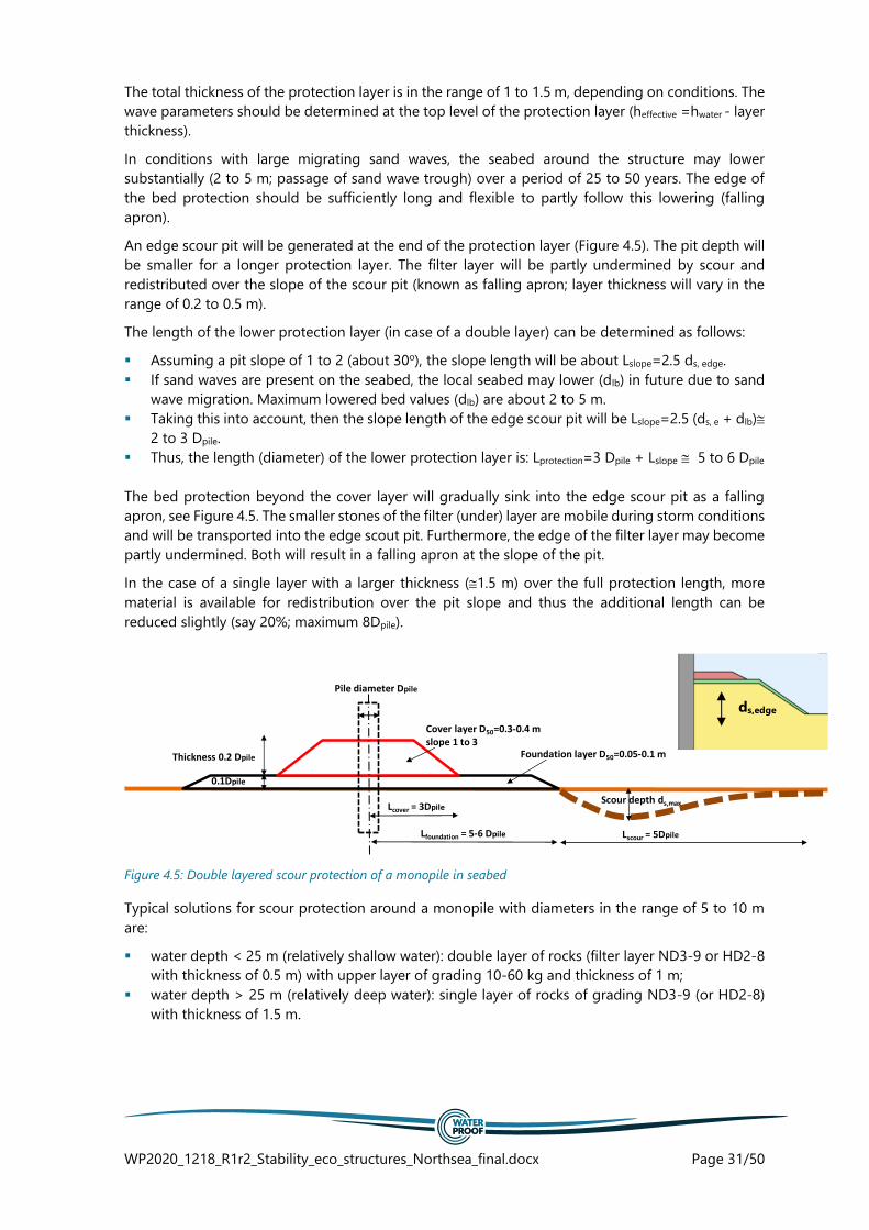
An edge scour pit will be generated at the end of the protection layer (Figure 4.5). The pit depth will
be smaller for a longer protection layer. The filter layer will be partly undermined by scour and
redistributed over the slope of the scour pit (known as falling apron; layer thickness will vary in the
range of 0.2 to 0.5 m).
The length of the lower protection layer (in case of a double layer) can be determined as follows:
▪ Assuming a pit slope of 1 to 2 (about 30o), the slope length will be about Lslope=2.5 ds, edge.
▪ If sand waves are present on the seabed, the local seabed may lower (dlb) in future due to sand
wave migration. Maximum lowered bed values (dlb) are about 2 to 5 m.
▪ Taking this into account, then the slope length of the edge scour pit will be Lslope=2.5 (ds, e + dlb)
2 to 3 Dpile.
▪ Thus, the length (diameter) of the lower protection layer is: Lprotection=3 Dpile + Lslope 5 to 6 Dpile
The bed protection beyond the cover layer will gradually sink into the edge scour pit as a falling
apron, see Figure 4.5. The smaller stones of the filter (under) layer are mobile during storm conditions
and will be transported into the edge scout pit. Furthermore, the edge of the filter layer may become
partly undermined. Both will result in a falling apron at the slope of the pit.
In the case of a single layer with a larger thickness (1.5 m) over the full protection length, more
material is available for redistribution over the pit slope and thus the additional length can be
reduced slightly (say 20%; maximum 8Dpile).
Figure 4.5: Double layered scour protection of a monopile in seabed
Typical solutions for scour protection around a monopile with diameters in the range of 5 to 10 m
are:
▪ water depth < 25 m (relatively shallow water): double layer of rocks (filter layer ND3-9 or HD2-8
with thickness of 0.5 m) with upper layer of grading 10-60 kg and thickness of 1 m;
▪ water depth > 25 m (relatively deep water): single layer of rocks of grading ND3-9 (or HD2-8)
with thickness of 1.5 m.
Lfoundation = 5-6 Dpile
Lcover = 3Dpile
Foundation layer D50=0.05-0.1 m
Cover layer D50=0.3-0.4 m slope 1 to 3
Pile diameter Dpile
Thickness 0.2 Dpile
0.1Dpile
Scour depth ds,max
Lscour = 5Dpile
ds,edge

WP2020_1218_R1r2_Stability_eco_structures_Northsea_final.docx Page 32/50
Table 4.3: Rock gradings (ND=normal density; HD=high density); rock sizes differ slightly for each quarry
Rock grading Median size [mm] Density [kg/m³] Type of layer
60-300 kg ND 470 (350-600) 2650 armour layer
40-200 kg ND 400 (300-520) 2650 armour layer
10-200 kg ND 350 (190-520) 2650 armour layer
10-60 kg ND 260 (190-350) 2650 armour layer
3-9 inch ND 125 (75-230) 2650 filter layer or single layer
3-9 inch HD 125 (75-230) 3000 filter layer or single layer
2-8 inch ND 100 (50-200) 2650 filter layer
2-8 inch HD 100 (50-200) 3050 filter layer
4.5 DESIGN SCOUR PROTECTION REEF STRUCTURE NORTH SEA
The tool ARMOUR has been used to predict the rock/stone sizes and associated damage level of the
scour protection layer during extreme current-wave conditions. Calculations have been made for the
Offshore Innovation lab and Borssele OWF separately, as the two locations differ significantly in
environmental conditions.
For the calculations, the following is assumed:
▪ width of the structure perpendicular to the current direction= 2 m;
▪ height of the structure (including foundation) = 2.5 m;
▪ stone density=2650 kg/m³;
▪ Shields critical mobility =0.025;
▪ velocity amplification factor near structure=1.2;
▪ a safety factor between 1 and 1.2;
▪ Damage: sd=1 start of damage and sd=2 minor damage
The results are shown in Table 4.4 and Table 4.5. The required stone size listed in these tables is the
median size requirement of the rock for the scour protection layer.
Table 4.4: Required stone size and associated damage level; Location: Borssele OWF.
Return
period
[years]
Water
depth
[m]
Water to MSL
[m]
Depth averaged
current velocity
[m/s] Significant
wave height
[m] and wave
period [s]
Safety factor = 1.2 Safety factor = 1
HWL LWL Flood
(to NE)
Eb (to
SW)
Required
Stone size
armour
layer [m]
sd for
1
storm
[-]
Required
Stone size
armour
layer [m]
sd for
1
storm
[-]
1 31 2.4 -1.8 1.1 1.08 5.22; 8.8 0.04 0.6 0.025 0.6
5 31 2.7 -1.95 1.19 1.12 6.15; 9.5 0.055 0.5 0.044 0.5
10 31 2.8 -2.05 1.22 1.14 6.57; 9.7 0.065 0.5 0.053 0.5
50 31 3.1 -2.2 1.30 1.17 7.50; 10.5 0.10 0.4 0.083 0.4
100 31 3.2 -2.25 1.33 1.19 7.87; 10.7 0.12 0.3 0.095 0.3
WP2020_1218_R1r2_Stability_eco_structures_Northsea_final.docx Page 33/50
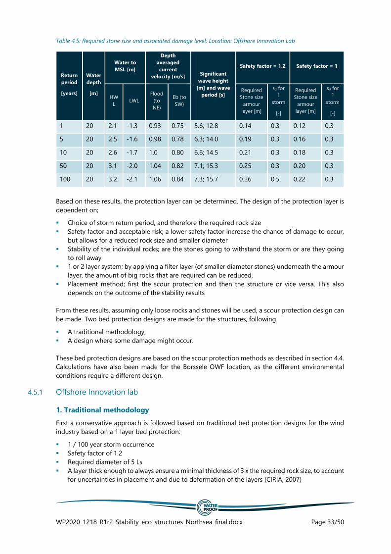
Table 4.5: Required stone size and associated damage level; Location: Offshore Innovation Lab
Return
period
[years]
Water
depth
[m]
Water to
MSL [m]
Depth
averaged
current
velocity [m/s] Significant
wave height
[m] and wave
period [s]
Safety factor = 1.2 Safety factor = 1
HW
L LWL
Flood
(to
NE)
Eb (to
SW)
Required
Stone size
armour
layer [m]
sd for
1
storm
[-]
Required
Stone size
armour
layer [m]
sd for
1
storm
[-]
1 20 2.1 -1.3 0.93 0.75 5.6; 12.8 0.14 0.3 0.12 0.3
5 20 2.5 -1.6 0.98 0.78 6.3; 14.0 0.19 0.3 0.16 0.3
10 20 2.6 -1.7 1.0 0.80 6.6; 14.5 0.21 0.3 0.18 0.3
50 20 3.1 -2.0 1.04 0.82 7.1; 15.3 0.25 0.3 0.20 0.3
100 20 3.2 -2.1 1.06 0.84 7.3; 15.7 0.26 0.5 0.22 0.3
Based on these results, the protection layer can be determined. The design of the protection layer is
dependent on;
▪ Choice of storm return period, and therefore the required rock size
▪ Safety factor and acceptable risk; a lower safety factor increase the chance of damage to occur,
but allows for a reduced rock size and smaller diameter
▪ Stability of the individual rocks; are the stones going to withstand the storm or are they going
to roll away
▪ 1 or 2 layer system; by applying a filter layer (of smaller diameter stones) underneath the armour
layer, the amount of big rocks that are required can be reduced.
▪ Placement method; first the scour protection and then the structure or vice versa. This also
depends on the outcome of the stability results
From these results, assuming only loose rocks and stones will be used, a scour protection design can
be made. Two bed protection designs are made for the structures, following
▪ A traditional methodology;
▪ A design where some damage might occur.
These bed protection designs are based on the scour protection methods as described in section 4.4.
Calculations have also been made for the Borssele OWF location, as the different environmental
conditions require a different design.
4.5.1 Offshore Innovation lab
1. Traditional methodology
First a conservative approach is followed based on traditional bed protection designs for the wind
industry based on a 1 layer bed protection:
▪ 1 / 100 year storm occurrence
▪ Safety factor of 1.2
▪ Required diameter of 5 Ls
▪ A layer thick enough to always ensure a minimal thickness of 3 x the required rock size, to account
for uncertainties in placement and due to deformation of the layers (CIRIA, 2007)

WP2020_1218_R1r2_Stability_eco_structures_Northsea_final.docx Page 34/50
Following the above mentioned assumptions, the protection layer is composed as follows:
▪ A required stone size in the range of 0.14 to 0.26 m; damage level below 1. This results in a
grading of 10-60 kg;
▪ A single layer with a thickness 1 m;
▪ Horizontal diameter=15 m.
The volume of stones can be calculated with:
𝑉 =𝜋
4 𝐷2 ℎ, with:
D = diameter of protection layer
h = thickness of protection layer
Combined this leads to a volume of stones 0.25xπx152x1=170 m3 270 tonnes;
Estimated costs: Euro 13,500 (Estimate of Euro 50,- per ton)
2. Design where some damage might occur
Because the bed protection is not designed for a wind foundation but for an eco-structure a less
conservative bed protection design might be enough. The following parameters settings are applied:
▪ 1 / 100 year storm occurrence
▪ Safety factor of 1
▪ 1 filter layer and 1 armour layer
▪ Required diameter of 3 to 4 Ls
▪ geotextile with diameter of 5 m attached to reef structure
▪ A layer thickness of about 2 x the required rock size (CIRIA, 2007).
Following the above mentioned parameter settings, the protection layer is composed as follows:
▪ A required stone size for the armour layer in the range of 0.12 to 0.22 m; damage level below 1.
This results in:
a grading of 10-60 kg;
a required thickness of 0.5 m
a horizontal diameter of 12 m;
▪ A required stone grading for the filter layer of 2-8 inch
With a required thickness of 0.3 m and a horizontal diameter of 12 m;
Combined this leads to a volume of stones0.25xπx122x0.5 + 0.25xπx122x0.3 =85 m3140 tonnes;
Estimated costs: Euro 7,000 (Estimate of Euro 50,- per ton)
4.5.2 Borssele OWF
1. Traditional methodology
Comparable to the Offshore Innovation lab site, first a conservative approach is followed for the
Borssele OWF site, based on traditional bed protection designs for the wind industry based on a 1
layer bed protection:
▪ 1 / 100 year storm occurrence
▪ Safety factor of 1.2
▪ Required diameter of area which should be protected of 5 Ls
▪ A layer thick enough to ensure a minimal thickness of 3 x the required rock size, to account for
uncertainties in placement and due to deformation of the layer (CIRIA, 2007)

WP2020_1218_R1r2_Stability_eco_structures_Northsea_final.docx Page 35/50
Following the above mentioned parameter settings, the protection layer is composed as follows:
▪ A required stone size in the range of 0.04 to 0.12 m; damage level below 1. This results in a
grading of 3-9 inch;
▪ A single layer with a thickness 0.75 m;
▪ Horizontal diameter=15 m.
Combined this leads to a volume of stones 0.25xπx152x0.75=125 m3 200 tonnes;
Estimated costs: Euro 10,000 (Estimate of Euro 50,- per ton)
2. Design where some damage might occur
Because the bed protection is not designed for a wind foundation but for an eco-structure a less
conservative bed protection design might be enough and some damage may take place. The
following parameters settings are applied:
▪ 1 / 100 year storm occurrence
▪ Safety factor of 1
▪ Required diameter of 3 to 4 Ls
▪ A layer thickness of about 2 x the required rock size, to have (minimal) insurance of a sufficient
thickness, even if stones start to roll away during storms or placement (CIRIA, 2007)
▪ geotextile with diameter of 5 m attached to reef structure
Following the above mentioned parameter settings, the design of the protection layer is as follows:
▪ A required stone size in the range of 0.03 to 0.10 m; damage level below 1. This results in a
grading of 2-8 inch;
▪ A single layer with a thickness 0.6 m;
▪ Horizontal diameter=10 m.
Combined this leads to a volume of stones 0.25xπx102x0.6 = 45 m3 75 tonnes;
Estimated costs: Euro 3,750 (Estimate of Euro 50,- per ton)
4.6 CONCLUSIONS
Bed protection
Based on the traditional methodology that we have applied above, a considerable bed protection
should be applied under the foreseen structures to guarantee no scour hole formation (see section
4.5). This is especially the case for the structure at the Offshore Innovation Lab, due to the presence
of more severe storm conditions, a smaller water depth and a smaller grainsize at the bed compared
to the OWF Borssele.
Accepted damage to bed protection in relation to design
When it is accepted that some damage may take place on the scour protection around the structures,
lower gradings of stones or smaller diameters of the protected area can be selected. This lowers the
height and volume of the required protection layer.
It is noted that this will also bring in risks which the Client should be aware of and include;
▪ Insufficient layer thickness because:
stones moved out of the protection layer during severe storms, or;
placement inaccuracies in relation to a relative thin layer thickness

WP2020_1218_R1r2_Stability_eco_structures_Northsea_final.docx Page 36/50
▪ Erosion because of insufficient layer thickness
scour erosion process can start through gaps between individual stones
▪ Stability of the structure on top of the scour protection
The movement of the armour layer could affect the stability of the structure if the structures
are placed directly on top of the protection layer.
Preventing stones to be transported out of the scour protection is especially important if the
structures are placed at the Borssele OWF location, due to the proximity to the cables and structures.
It is up to the Client if damage is accepted or not and which of the provided scour protection designs
will be applied.
Application of shells
De Rijke Noordzee intends to mix shells through the scour protection. It is noted that the application
of shells does not reduce the scour protection size. Shells (especially lighter mussel shells) start to
move at relative low flow velocities compared to rock protection. We therefore advise:
▪ If applied, best method would be to mix the shells with the stones before placing to minimize
outwashing (in any case the upper shells will be washed out)
▪ If used a low quantity is recommended, to limit the total layer thickness

WP2020_1218_R1r2_Stability_eco_structures_Northsea_final.docx Page 37/50
5 STABILITY
5.1 INTRODUCTION
In this chapter the stability of the structures is assessed. The interaction between the hydraulic forces
and structures can result in 2 failure mechanisms; failure due to turning over and failure due to
movement out of foundation, see Figure 5.1.
For mechanism 1, the moments (Force x distance) on the structures are of importance. Whether or
not the structure turns over depends on the balance of the acting moment by the flow/waves, and
the counteracting moment due to the weight of the structure itself. The acting moment is the product
of the force and its application point as determined by the Morison equation, as is explained in
Section 5.2. The counteracting moment depends on the weight of the structure and the distance a2:
this is the distance from the centre of the structure to the turning point (see figure 5.1).
Apart from structure turning over, the structures can be pushed out of the foundation area
(mechanism 2, see right panel in Figure 5.1). Here, the balance between the horizontal force against
the construction and the shear stresses between foundation and construction is of importance. The
maximum shear stress (just before sliding occurs) depends on the weight of the structure, size and
roughness of the structure, and roughness of the foundation layer.
In addition to these two failure mechanisms, the combined weight of the structure could exceed the
bearing capacity of the soil, causing (uneven) settling, risking inducing mechanism 1 earlier than first
estimated. All failure mechanisms are addressed in this chapter.
Figure 5.1: Failure mechanisms considered
5.2 FORCES ON THE STRUCTURE
A worldwide used method to calculate forces under a combination of currents and waves is the
(adapted) Morison equation. The Morison equation is the sum of two force components: an inertia
force in phase with the local flow acceleration and a drag force proportional to the (signed) square
of the instantaneous flow velocity. The inertia force is of the functional form as found in potential
flow theory, while the drag force has the form as found for a body placed in a steady flow.
𝐹 = 𝜌 𝐶𝑀 𝑉 𝑎 +1
2 𝜌 𝐶𝐷 𝐴 𝑢 | 𝑢 |, where:
𝜌 = density of water,
CM = inertia coefficient,
V = volume of the structure,
a = acceleration at the structure,

WP2020_1218_R1r2_Stability_eco_structures_Northsea_final.docx Page 38/50
CD = drag coefficient,
u = flow velocities approaching the structure
It can be said that the stability of the reef structures depends on:
▪ The fluid flow velocities approaching the structure;
▪ The fluid accelerations at the structure due to waves;
▪ The effective surface area normal to the flow;
▪ The volume of the structure;
▪ The hydraulic drag coefficient (CD) and the inertia coefficient (CM);
▪ The distance of the centre of the structure to the turning point (a2), only relevant for mechanism
1;
▪ The friction of the seabed / scour protection.
The first four points are dependent on the design and placement alone. The drag coefficient can be
determined with laboratory experiments. The inertia and friction coefficients can be determined on
literature.
The highest uncertainties in the equation lie in the drag coefficient Cd and the distance a2:
▪ The drag coefficient CD is only known for single standard elements such as spheres, cubes,
cylinders, etc. and not for the proposed structure. Moreover, effects of marine growth affect
this drag coefficient, where a rougher surface increases the drag.
▪ The distance a2. When the structure is placed on a fixed seabed the turning point will be
located as shown in Figure 5.1. However, when the bed can deform (which is the case for a
gravel layer on sand or due to uneven settling) the location of the turning point shifts
towards G, making a2 shorter and the ability of the structure to turn over larger.
Of these two parameters, the uncertainties regarding drag coefficient CD can be minimized by
performing laboratory tests. Therefore, in-house flume experiments have been executed. These
experiments are performed within our 5 m long flow-flume. The results of these experiments are
described in Section 5.3. The resulting parameters CD is used in the stability calculation in Section 5.4.
5.3 LABORATORY TESTS
To gain insight in the magnitude of the drag coefficients of the structures, the following flume
experiments have been performed:
▪ One individual block only for 2 densities (2 experiments)
▪ Structure Type A in 2 orientations and for 2 densities (3 experiments)
We have conducted the flow flume experiments at a scaling of 1:10 (single block) and 1:17 (structure).
Generally applicable scale rules have been used to scale the structures to representative dimensions.
The flow velocity in the flume is increased from 0 to approx. 0.85 m/s in steps until the structure
becomes unstable and turns over (critical conditions) and/or starts to slide. The vertical distribution
of the fluid velocities is measured using an electro-magnetic current meter. The structures are made
of material with a density which is equivalent to the concrete of the actual structures. The density of
the material of the foundation layer is comparable to the density of the actual bed protection.
The two different mechanisms require two different methods of calculating the drag coefficient:
With the weight of the structure and the turning arm known, the counteracting moment of
mechanism 1 is determined. When the structure just becomes unstable, this counteracting
moment balances out the force that the flow exerts on the structure. This force is calculated with
the Morison formula as explained in section 5.2; assuming the accelerations are 0, the only
unknown parameter is the drag coefficient.

WP2020_1218_R1r2_Stability_eco_structures_Northsea_final.docx Page 39/50
With the weight of the structure and the friction coefficient of the flume known, the friction
force of mechanism 2 is determined. When the structure just starts to slide, this force is exactly
equal to the force that the flow exerts on the structure. This force is again calculated with the
Morison formula as explained in section 5.2; assuming the accelerations are 0, the only unknown
parameter is the drag coefficient.
Figure 5.2 shows the snapshot of the initiation of mechanism 1 (tipping over) for structure design A,
for two different orientations with respect to the flow direction. Table 5.1 shows the results of the
flume tests, such as the speeds at which the mechanisms occur and the accompanying drag
coefficient for all structures.
Figure 5.2: Top: flow flume set-up. Bottom: two examples of initiation of mechanism 1, for the light weight
structures with 2 different orientations in the flow direction. The flow direction in both cases is from left to right.
Table 5.1: Results of the flume tests, showing the maximum flow velocities at which the structures start to slide and
turn over. Combined with the volume and density of the material, the drag coefficient CD is determined.
Structure
Density
material
[g/cc]
Volume
of
structure
[mL]
Mechanism 1 Mechanism 2
CD [-] Max. flow
for turning
over [m/s]
Water
depth
[cm]
Max. flow
for sliding
[m/s]
Water
depth
[cm]
1 individual block
0.1 1.27 75 0.28 16 0.20 16 1.54
+- 0.005
0.2 3.22 75 0.81 16 0.57 16 1.66
+- 0.00

WP2020_1218_R1r2_Stability_eco_structures_Northsea_final.docx Page 40/50
Structure
Density
material
[g/cc]
Volume
of
structure
[mL]
Mechanism 1 Mechanism 2
CD [-] Max. flow
for turning
over [m/s]
Water
depth
[cm]
Max. flow
for sliding
[m/s]
Water
depth
[cm]
Combined structures
A.1, wide
side ⊥ flow 1.33 175 0.25 16 0.18 16
2.17
+- 0.00
A.1, narrow
side ⊥ flow 1.33 175 0.32 16 0.20 16
2.11
+- 0.03
A.2, wide
side ⊥ flow 3.20 175 0.68 15 0.48 16
1.84-
2.09
5.4 STABILITY CALCULATION
There are several important parameters in the calculations of the two failure mechanisms. Based on
the laboratory results and literature studies, the following can be said:
▪ Drag coefficient, CD
The laboratory results show that this parameter has a varying value between 1.6 (smooth
singular block) to 2.2 (structure with widest part perpendicular to the current direction. It is
important to mention that the application of additional attachments to the structure or marine
growth can further increase the value of this parameter. In order to take marine growth still into
account, it is assumed that marine growth will increase the width of the structure by 10 cm at
all sides.
▪ Distance to turning point, a2 :
The distance a2 equals the distance between the location of the centre of gravity and the turning
point. This value is maximum when the turning point is at the corner of the structure. Therefore,
the maximum value equals half of width parallel to flow. However, if structure placed on top of
scour protection, uneven stone distribution or angled stones can lower this distance significantly
by moving the turning point closer to the centre of the structure. Additionally, if the combined
weight of the structure and the protection exceed bearing capacity, (uneven) settling could
induce additional slope, which also lowers the distance.
For the calculations performed in this paragraph, the distance is assumed to be maximum. But,
in order to account for the uncertainties, a safety factor is applied.
▪ Inertia coefficient, CM:
This coefficient depends on the added mass to the structure; the extra inertia the structure will
feel when water is accelerated (or decelerated). This dependence is expressed as (Bai, 2005):
CM = Ca + 1
The presence of a fixed boundary has a pronounced effect on the inertia (and the added mass)
coefficient; the smaller the distance to the bed, the larger this parameter becomes. As the
structure is placed at the seabed, Ca becomes equal to 2. With the aforementioned dependence
between the inertia coefficient and the added mass coefficient Ca, CM therefore becomes equal
to 3.
▪ Friction of bed, friction parameter μd
The bed friction is an important parameter that determines the moment when sliding is initiated.
The friction resulting from the weight of the structure is as follows:

WP2020_1218_R1r2_Stability_eco_structures_Northsea_final.docx Page 41/50
Ffriction = Fweight * μd, with,
Fweight = (ρstructure-ρwater)*Volume structure* g
ρstructure = 2130 [kg/m3]
ρwater = 1025 [kg/m3] (salt water)
g = 9.81 [m/s2]
μd = dynamic friction coefficient
The friction coefficient can be interpreted as follows; the lower the value is, the lower the friction
force becomes, the easier it is for the structure to start sliding. Several studies have looked into
the friction coefficient for sand. Depending on the sand type and its moisture contents (Fall,
2014) this value can vary. For wet sand, the friction value equals between 0.4 and 0.5. Our flume
for example has a friction coefficient equal to 0.46. It is expected however, that in reality the
structure will not slide smoothly, but will push itself into the sand / the scour protection layer.
Additionally, rocks have a higher friction coefficient than sand. Therefore, this study assumes
the friction coefficient to be equal to 0.6.
From the above, it can be said that there are still a number of uncertainties; especially with respect
to the drag parameter and the distance to the turning point. Based on these uncertainties a total
safety factor of 1.2 is applied in the stability calculation for conservatism reasons.
5.4.1 Forces on the structures
Based on the above, the forces on the structures and moments due to these forces on the structures
are calculated. Table 5.2 shows the results of these calculations for placement at the Offshore
Innovation Lab. Table 5.3 shows the results of the calculations if the structures are placed at the OWF
Borssele location.
Apart from the afore mentioned structure options A and B, an additional calculation is made for a
fully symmetrical version of option A, with either a 3 x 3 blocks base or a 4 x 4 blocks base. This
calculation is made as the placement of the structures (wide or narrow side in the flow) cannot be
guaranteed offshore and the calculations are thus based on the most unfavourable orientation. With
a symmetrical structure the result of the calculation is not affected by orientation (results are the
same for all sides) .
It can be seen that the forces and their resulting moments at the Offshore Innovation Lab are larger
than at the OWF Borssele location. This difference can be explained by the smaller depth at the
Offshore Innovation Lab, as the hydrodynamic conditions between the two locations are similar. Due
to this smaller depth (and the structure height to depth ratio) it is easier for the forces to ‘grab onto’
the structure.
Table 5.2: Resulting forces and moments on the structure based on the Morison calculations. Location: Offshore
Innovation Lab
Structure
Return period [years]
1 5 10 50 100
F
[kN]
M
[kNm]
F
[kN]
M
[kNm]
F
[kN]
M
[kNm]
F
[kN]
M
[kNm]
F
[kN]
M
[kNm]
A, wide 15.5 12.1 19.4 16.2 22.7 18.5 25.6 22.0 27.6 23.9
A, narrow 14.1 11.7 17.6 15.5 20.4 17.7 23.1 21.1 24.8 22.9
B, wide 12.9 8.4 16.1 11.2 19.0 12.9 21.2 15.2 22.9 16.6
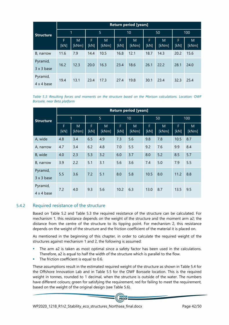
WP2020_1218_R1r2_Stability_eco_structures_Northsea_final.docx Page 42/50
Structure
Return period [years]
1 5 10 50 100
F
[kN]
M
[kNm]
F
[kN]
M
[kNm]
F
[kN]
M
[kNm]
F
[kN]
M
[kNm]
F
[kN]
M
[kNm]
B, narrow 11.6 7.9 14.4 10.5 16.8 12.1 18.7 14.3 20.2 15.6
Pyramid,
3 x 3 base 16.2 12.3 20.0 16.3 23.4 18.6 26.1 22.2 28.1 24.0
Pyramid,
4 x 4 base 19.4 13.1 23.4 17.3 27.4 19.8 30.1 23.4 32.3 25.4
Table 5.3: Resulting forces and moments on the structure based on the Morison calculations. Location: OWF
Borssele, near Beta platform
Structure
Return period [years]
1 5 10 50 100
F
[kN]
M
[kNm]
F
[kN]
M
[kNm]
F
[kN]
M
[kNm]
F
[kN]
M
[kNm]
F
[kN]
M
[kNm]
A, wide 4.8 3.4 6.5 4.9 7.3 5.6 9.8 7.8 10.5 8.7
A, narrow 4.7 3.4 6.2 4.8 7.0 5.5 9.2 7.6 9.9 8.4
B, wide 4.0 2.3 5.3 3.2 6.0 3.7 8.0 5.2 8.5 5.7
B, narrow 3.9 2.2 5.1 3.1 5.6 3.6 7.4 5.0 7.9 5.5
Pyramid,
3 x 3 base 5.5 3.6 7.2 5.1 8.0 5.8 10.5 8.0 11.2 8.8
Pyramid,
4 x 4 base 7.2 4.0 9.3 5.6 10.2 6.3 13.0 8.7 13.5 9.5
5.4.2 Required resistance of the structure
Based on Table 5.2 and Table 5.3 the required resistance of the structure can be calculated. For
mechanism 1, this resistance depends on the weight of the structure and the moment arm a2; the
distance from the centre of the structure to its tipping point. For mechanism 2, this resistance
depends on the weight of the structure and the friction coefficient of the material it is placed on.
As mentioned in the beginning of this chapter, in order to calculate the required weight of the
structures against mechanism 1 and 2, the following is assumed:
▪ The arm a2 is taken as most optimal since a safety factor has been used in the calculations.
Therefore, a2 is equal to half the width of the structure which is parallel to the flow.
▪ The friction coefficient is equal to 0.6.
These assumptions result in the estimated required weight of the structure as shown in Table 5.4 for
the Offshore Innovation Lab and in Table 5.5 for the OWF Borssele location. This is the required
weight in tonnes, rounded to 1 decimal, when the structure is outside of the water. The numbers
have different colours; green for satisfying the requirement, red for failing to meet the requirement,
based on the weight of the original design (see Table 5.6).

WP2020_1218_R1r2_Stability_eco_structures_Northsea_final.docx Page 43/50
Table 5.4: Required weight to counter the calculated forces for sliding and tipping over of the different structures,
for the different return periods. Location: Offshore Innovation Lab. The numbers are red if the required weight is
larger than the actual weight of the structure (requirement is not met) and green if the required weight is smaller
than the actual weight of the structure (requirement is met).
Structure
Return period [years]
1 5 10 50 100
Slide
[t]
Turn
[t]
Slide
[t]
Turn
[t]
Slide
[t]
Turn
[t]
Slide
[t]
Turn
[t]
Slide
[t]
Turn
[t]
A, wide 5.1 8 6.4 10.6 7.5 12.2 8.4 14.5 9.1 15.7
A, narrow 4.7 5.1 5.8 6.8 6.7 7.8 7.6 9.3 8.2 10
B, wide 4.3 5.5 5.3 7.4 6.3 8.5 7 10 7.6 10.9
B, narrow 3.8 3.5 4.8 4.7 5.5 5.3 6.2 6.3 6.7 6.9
Pyramid,
3 x 3 base 5.3 5.4 6.6 7.2 7.7 8.2 8.6 9.7 9.3 10.5
Pyramid,
4 x 4 base 6.4 4.3 7.7 5.7 9 6.5 9.9 7.7 10.6 8.4
Table 5.5: Required weight to counter the calculated forces for sliding and turning over of the different structures,
for the different return periods. Location: OWF Borssele, near Beta platform. The numbers are red if the required
weight is larger than the actual weight of the structure (requirement is not met) and green if the required weight
is smaller than the actual weight of the structure (requirement is met).
Structure
Return period [years]
1 5 10 50 100
Slide
[t]
Turn
[t]
Slide
[t]
Turn
[t]
Slide
[t]
Turn
[t]
Slide
[t]
Turn
[t]
Slide
[t]
Turn
[t]
A, wide 1.6 2.3 2.2 3.3 2.4 3.7 3.3 5.2 3.5 5.7
A, narrow 1.6 1.5 2.1 2.1 2.3 2.4 3.1 3.4 3.3 3.7
B, wide 1.4 1.5 1.8 2.2 2 2.5 2.7 3.5 2.8 3.8
B, narrow 1.3 1 1.7 1.4 1.9 1.6 2.5 2.2 2.6 2.4
Pyramid,
3 x 3 base 1.8 1.6 2.4 2.3 2.7 2.6 3.5 3.5 3.7 3.9
Pyramid,
4 x 4 base 2.4 1.4 3.1 1.9 3.4 2.1 4.3 2.9 4.5 3.2
The estimated weight of the individual structures, with only the top (option B) / or the top two cubes
(option A) filled with smaller cubes is shown in Table 5.6. It is assumed that the cubes have a density
of light weight concrete (2150 kg/m3) and are filled with a comparable type of material with a 30%
porosity.
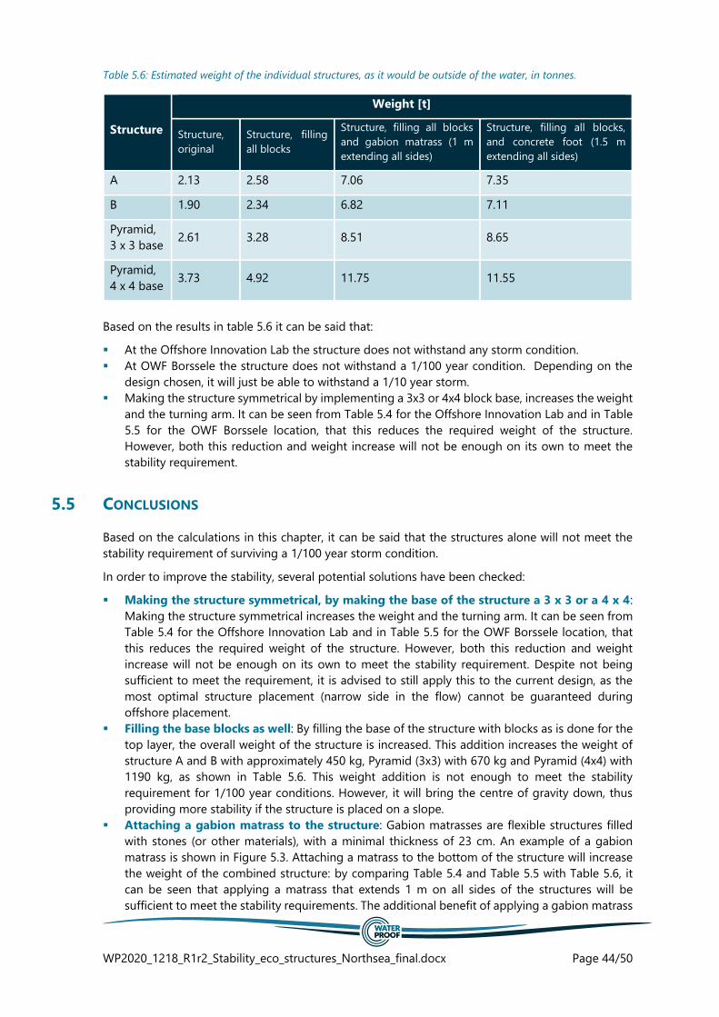
WP2020_1218_R1r2_Stability_eco_structures_Northsea_final.docx Page 44/50
Table 5.6: Estimated weight of the individual structures, as it would be outside of the water, in tonnes.
Structure
Weight [t]
Structure,
original
Structure, filling
all blocks
Structure, filling all blocks
and gabion matrass (1 m
extending all sides)
Structure, filling all blocks,
and concrete foot (1.5 m
extending all sides)
A 2.13 2.58 7.06 7.35
B 1.90 2.34 6.82 7.11
Pyramid,
3 x 3 base 2.61 3.28 8.51 8.65
Pyramid,
4 x 4 base 3.73 4.92 11.75 11.55
Based on the results in table 5.6 it can be said that:
▪ At the Offshore Innovation Lab the structure does not withstand any storm condition.
▪ At OWF Borssele the structure does not withstand a 1/100 year condition. Depending on the
design chosen, it will just be able to withstand a 1/10 year storm.
▪ Making the structure symmetrical by implementing a 3x3 or 4x4 block base, increases the weight
and the turning arm. It can be seen from Table 5.4 for the Offshore Innovation Lab and in Table
5.5 for the OWF Borssele location, that this reduces the required weight of the structure.
However, both this reduction and weight increase will not be enough on its own to meet the
stability requirement.
5.5 CONCLUSIONS
Based on the calculations in this chapter, it can be said that the structures alone will not meet the
stability requirement of surviving a 1/100 year storm condition.
In order to improve the stability, several potential solutions have been checked:
▪ Making the structure symmetrical, by making the base of the structure a 3 x 3 or a 4 x 4:
Making the structure symmetrical increases the weight and the turning arm. It can be seen from
Table 5.4 for the Offshore Innovation Lab and in Table 5.5 for the OWF Borssele location, that
this reduces the required weight of the structure. However, both this reduction and weight
increase will not be enough on its own to meet the stability requirement. Despite not being
sufficient to meet the requirement, it is advised to still apply this to the current design, as the
most optimal structure placement (narrow side in the flow) cannot be guaranteed during
offshore placement.
▪ Filling the base blocks as well: By filling the base of the structure with blocks as is done for the
top layer, the overall weight of the structure is increased. This addition increases the weight of
structure A and B with approximately 450 kg, Pyramid (3x3) with 670 kg and Pyramid (4x4) with
1190 kg, as shown in Table 5.6. This weight addition is not enough to meet the stability
requirement for 1/100 year conditions. However, it will bring the centre of gravity down, thus
providing more stability if the structure is placed on a slope.
▪ Attaching a gabion matrass to the structure: Gabion matrasses are flexible structures filled
with stones (or other materials), with a minimal thickness of 23 cm. An example of a gabion
matrass is shown in Figure 5.3. Attaching a matrass to the bottom of the structure will increase
the weight of the combined structure: by comparing Table 5.4 and Table 5.5 with Table 5.6, it
can be seen that applying a matrass that extends 1 m on all sides of the structures will be
sufficient to meet the stability requirements. The additional benefit of applying a gabion matrass
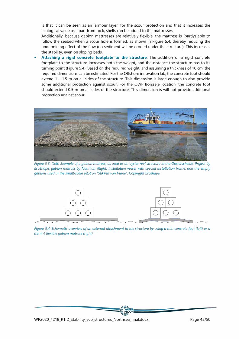
WP2020_1218_R1r2_Stability_eco_structures_Northsea_final.docx Page 45/50
is that it can be seen as an ‘armour layer’ for the scour protection and that it increases the
ecological value as, apart from rock, shells can be added to the mattresses.
Additionally, because gabion mattresses are relatively flexible, the mattress is (partly) able to
follow the seabed when a scour hole is formed, as shown in Figure 5.4, thereby reducing the
undermining effect of the flow (no sediment will be eroded under the structure). This increases
the stability, even on sloping beds.
▪ Attaching a rigid concrete footplate to the structure: The addition of a rigid concrete
footplate to the structure increases both the weight, and the distance the structure has to its
turning point (Figure 5.4). Based on the required weight, and assuming a thickness of 10 cm, the
required dimensions can be estimated. For the Offshore innovation lab, the concrete foot should
extend 1 – 1.5 m on all sides of the structure. This dimension is large enough to also provide
some additional protection against scour. For the OWF Borssele location, the concrete foot
should extend 0.5 m on all sides of the structure. This dimension is will not provide additional
protection against scour.
Figure 5.3: (Left) Example of a gabion matrass, as used as an oyster reef structure in the Oosterschelde. Project by
EcoShape, gabion matrass by Nautilus. (Right) Installation vessel with special installation frame, and the empty
gabions used in the small-scale pilot on “Slikken van Viane”. Copyright Ecoshape.
Figure 5.4: Schematic overview of an external attachment to the structure by using a thin concrete foot (left) or a
(semi-) flexible gabion matrass (right).

WP2020_1218_R1r2_Stability_eco_structures_Northsea_final.docx Page 46/50
6 CONCLUSIONS AND
RECOMMENDATIONS FOR DESIGN
OPTIMIZATION
6.1 CONCLUSIONS
Based on the scour and stability calculations the following can be concluded.
6.1.1 Scour protection
Based on the traditional methodology that we have applied above, a considerable bed protection
should be applied under the foreseen structures to guarantee no scour hole formation (see 4.5). This
is especially the case for the structure at the Offshore Innovation Lab, due to the presence of more
severe storm conditions, a smaller water depth and a smaller grainsize at the bed compared to the
OWF Borssele.
Accepted damage to bed protection in relation to design
When it is accepted that some damage may take place on the scour protection around the structures,
lower gradings of stones or smaller diameters of the protected area can be selected. This lowers the
height and volume of the required protection layer.
It is noted that this will also bring in risks which the Client should be aware of and include;
▪ Insufficient layer thickness because:
stones moved out of the protection layer during severe storms, or;
placement inaccuracies in relation to a relative thin layer thickness
▪ Erosion because of insufficient layer thickness
scour erosion process can start through gaps between individual stones
▪ Stability of the structure on top of the scour protection
The movement of the armour layer could affect the stability of the structure if the structures
are placed directly on top of the protection layer.
Preventing stones to be transported out of the scour protection is especially important if the
structures are placed at the Borssele OWF location, due to the proximity to the cables and structures.
It is up to the Client if damage is accepted or not and which of the provided scour protection designs
will be applied.
Application of shells
De Rijke Noordzee intends to mix shells through the scour protection. It is noted that the application
of shells does not reduce the scour protection size. Shells (especially lighter mussel shells) start to
move at relative low flow velocities compared to rock protection. We therefore advise:
▪ If applied, best method would be to mix the shells with the stones before placing to minimize
outwashing (in any case the upper shells will be washed out)
If used a low quantity is recommended, to limit the total layer thickness

WP2020_1218_R1r2_Stability_eco_structures_Northsea_final.docx Page 47/50
6.1.2 Stability
The flow flume experiments have been very useful to decrease the uncertainties of the stability
calculations. Because also with help of the flow flume experiments still uncertainties remain, a total
safety factor of 1.2 is applied in the stability calculation for conservatism reasons.
It is concluded that the forces and their resulting moments at the Offshore Innovation Lab are larger
than at the OWF Borssele location. This difference can be explained by the smaller depth at the
Offshore Innovation Lab, as the hydrodynamic conditions between the two locations are similar. Due
to this smaller depth (and the structure height to depth ratio) it is easier for the forces to ‘grab onto’
the structure.
Based on the calculations in this chapter, it can be said that:
▪ When placed at the Offshore Innovation Lab the structure does not withstand any storm
condition.
▪ If placed at OWF Borssele the structure does not withstand a 1/100 year condition. Depending
on the design chosen, it will just be able to withstand a 1/10 year storm.
In the section below, recommendations are given to increase the stability of the structures.
6.2 RECOMMENDATIONS FOR DESIGN OPTIMIZATION
6.2.1 Optimization of location
In order to minimize the risk of not meeting the stability requirements, the location for the structures
should be chosen as such that:
▪ The slope of the bed is as small as possible
▪ Sandwaves do not impose a risk on the structure
It is therefore advised that:
▪ The structures are placed at least 200 m away from the crests of the nearby sandwaves to take
the migration rates into account;
▪ The structures are placed on the location with a small slope, thus the sand wave crest should be
avoided;
▪ The sandwave through is the lowest point in the surrounding seabed and will fill up over time,
thus it should be avoided.
Additionally, the Offshore Innovation Lab is located nearby a disposal site of silty sediments. In order
limit the potential siltation of the structures and to have a stable subsoil, the structure should be
placed as far away as possible from this site (towards the NW corner).
6.2.2 Optimization structures and scour protection
Based on the results of chapter 4 and 5, it can be said that the stability requirements are not met,
and that a severe scour hole will be formed which will have a negative effect on the stability if no
scour protection will be used.
In order to prevent the structure from sinking into the seabed / tipping over early due to scour, scour
protection is required. Depending on the acceptable risk, a different design is proposed.
In order to guarantee the stability of the structures themselves, weight has to be added to the
structure. Potential solutions regarding the stability are:

WP2020_1218_R1r2_Stability_eco_structures_Northsea_final.docx Page 48/50
Making the structure symmetrical
Making the structure symmetrical increases the weight and the turning arm. It can be seen from
Table 5.4 for the Offshore Innovation Lab and in Table 5.5 for the OWF Borssele location, that this
reduces the required weight of the structure. However, both this reduction and weight increase will
not be enough on its own to meet the stability requirement. Despite not being sufficient to meet the
requirement, it is advised to still apply this to the current design, as the most optimal structure
placement (narrow side in the flow) cannot be guaranteed during offshore placement.
Filling the base blocks
By filling the base of the structure with blocks as is done for the top tiers, the overall weight of the
structure is increased. This addition increases the weight of structure A and B with approximately 450
kg, Pyramid (3x3) with 670 kg and Pyramid (4x4) with 1190 kg, as shown in Table 5.6. This weight
addition is not enough to meet the stability requirement for 1/100 year conditions. However, it will
bring the centre of gravity down, thus providing more stability if the structure is placed on a slope.
Attaching external weight to the structure
When extra weight is added to the structure the stability increases. This can be done in various ways.
Two examples are explained in more detail below.
Gabion matrasses are flexible structures filled with stones (or other materials), with a minimal
thickness of 23 cm. Attaching a matrass to the bottom of the structure will increase the weight of the
combined structure: applying a matrass that extends 1 m on all sides of the structures will be
sufficient to meet the stability requirements. The additional benefit of applying a gabion matrass is
that it can be seen as an ‘armour layer’ for the scour protection and that it increases the ecological
value as, apart from rock, shells can be added to the mattresses.
Additionally, because gabion mattresses are relatively flexible, the mattress is (partly) able to follow
the seabed when a scour hole is formed, thereby reducing the undermining effect of the flow (no
sediment will be eroded under the structure). This increases the stability, even on sloping beds.
Attaching a rigid concrete footplate to the structure: the addition of a rigid concrete foot to the
structure increases both the weight, and the distance the structure has to its turning point. Based on
the required weight, and assuming a thickness of 10 cm, for the Offshore innovation lab, the concrete
foot should extend 1.5 m on all sides of the structure. This dimension is large enough to also provide
some additional protection against scour. For the OWF Borssele location, the concrete foot should
extend 0.5 m on all sides of the structure.
The 2 mentioned solutions below provide additional protection against scour as well. If one of these
solutions are chosen, it is advised to re-evaluate the required scour protection dimensions as
provided under Chapter 4. Best option would be to first place the structure including concrete plate/
gabion mattress and next place a layer of scour protection on the mattress/ slab. In this way the
integrity of the combined structure (scour protection & structure) is further increased.
6.2.3 Optimization of installation method
The different suggested optimizations require different installation methods and different installation
vessels. This is true for both the suggested scour protection, and the installation of the structure
itself.
With regards to the installation of loose scour protection (e.g. the stones), several methods and
corresponding installation vessels are available. Examples of 3 of such installation vessels are:
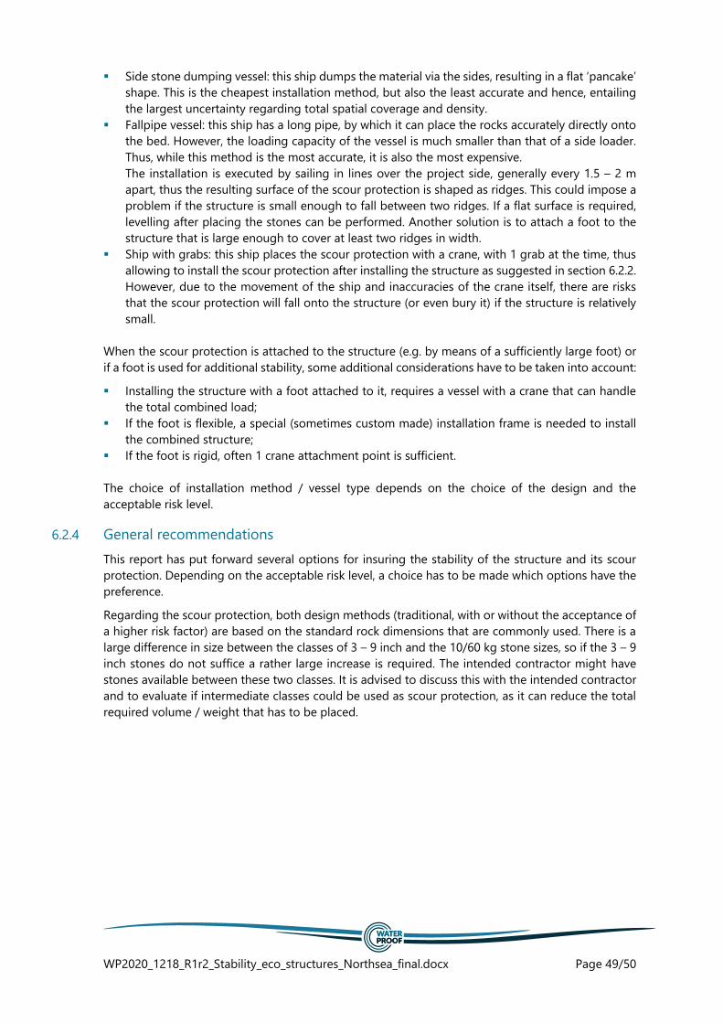
WP2020_1218_R1r2_Stability_eco_structures_Northsea_final.docx Page 49/50
▪ Side stone dumping vessel: this ship dumps the material via the sides, resulting in a flat ‘pancake’
shape. This is the cheapest installation method, but also the least accurate and hence, entailing
the largest uncertainty regarding total spatial coverage and density.
▪ Fallpipe vessel: this ship has a long pipe, by which it can place the rocks accurately directly onto
the bed. However, the loading capacity of the vessel is much smaller than that of a side loader.
Thus, while this method is the most accurate, it is also the most expensive.
The installation is executed by sailing in lines over the project side, generally every 1.5 – 2 m
apart, thus the resulting surface of the scour protection is shaped as ridges. This could impose a
problem if the structure is small enough to fall between two ridges. If a flat surface is required,
levelling after placing the stones can be performed. Another solution is to attach a foot to the
structure that is large enough to cover at least two ridges in width.
▪ Ship with grabs: this ship places the scour protection with a crane, with 1 grab at the time, thus
allowing to install the scour protection after installing the structure as suggested in section 6.2.2.
However, due to the movement of the ship and inaccuracies of the crane itself, there are risks
that the scour protection will fall onto the structure (or even bury it) if the structure is relatively
small.
When the scour protection is attached to the structure (e.g. by means of a sufficiently large foot) or
if a foot is used for additional stability, some additional considerations have to be taken into account:
▪ Installing the structure with a foot attached to it, requires a vessel with a crane that can handle
the total combined load;
▪ If the foot is flexible, a special (sometimes custom made) installation frame is needed to install
the combined structure;
▪ If the foot is rigid, often 1 crane attachment point is sufficient.
The choice of installation method / vessel type depends on the choice of the design and the
acceptable risk level.
6.2.4 General recommendations
This report has put forward several options for insuring the stability of the structure and its scour
protection. Depending on the acceptable risk level, a choice has to be made which options have the
preference.
Regarding the scour protection, both design methods (traditional, with or without the acceptance of
a higher risk factor) are based on the standard rock dimensions that are commonly used. There is a
large difference in size between the classes of 3 – 9 inch and the 10/60 kg stone sizes, so if the 3 – 9
inch stones do not suffice a rather large increase is required. The intended contractor might have
stones available between these two classes. It is advised to discuss this with the intended contractor
and to evaluate if intermediate classes could be used as scour protection, as it can reduce the total
required volume / weight that has to be placed.
WP2020_1218_R1r2_Stability_eco_structures_Northsea_final.docx Page 50/50
7 REFERENCES
Bai, Y., & Bai, Q. (Eds.). (2005). Subsea pipelines and risers. Elsevier.
COAST (2019). Characterisation of a Monopile Scour Protection System.
Construction Industry Research, Information Association, Civieltechnisch Centrum Uitvoering
Research en Regelgeving (Netherlands), & Centre d'études maritimes et fluviales (France). (2007).
The rock manual: the use of rock in hydraulic engineering (Vol. 683). Ciria.
Deltares (2015). Site Studies Wind Farm Zone Borssele, MetOcean study for the Borssele Wind Farm
Zone Site III.
Deltares (2016a). Morphodynamics of Borssele Wind Farm Zone WFS-IV, WFS-III and WFS-V. Update
version January 25th, 2016
Deltares (2016b). Morphodynamics of Hollandse Kust (Zuid) Wind Farm Zone
Deltares (2016c). Borssele OHVS – Scour and scour protection
DHI (2017). MetOcean Study, Hollandse Kust Wind Farm Zone. Version September 2017
Fall, A., Weber, B., Pakpour, M., Lenoir, N., Shahidzadeh, N., Fiscina, J., ... & Bonn, D. (2014). Sliding
friction on wet and dry sand. Physical review letters, 112(17), 175502.
Fugro (2016). Final report geophysical and geotechnical site investigation survey 150116, Offshore
NL Borssele.
Fugro (2017). Hollandse Kust Zuid, Marine Geophysical & Geotechnical Route Surveys.
Hjorth, P. (1975). Studies on the nature of local scour. Inst. för Teknisk Vattenresurslära, Lunds
Tekniska Högskola, Lunds Univ..
Munoz-Peres, J.J., et al. (2015). Sinking of concrete modules into a sandy seabed: a case
study. Coastal Engineering, Vol. 99, 26-37
WaterProof (2015). Seabed mobility based burial depth assessment Borssele cable.
WaterProof (2017). Seabed mobility update, Wind op Zee – Hollandse Kust Zuid export cable.
Whitehouse, R. J. (2004). Marine scour at large foundations.
Svasek (2016). Metoceandata export cables Hollandse Kust Zuid, Methodology and model validation.
Tavouktsoglou, N. S., Harris, J. M., Simons, R. R., & Whitehouse, R. J. S. (2017). Equilibrium scour-
depth prediction around cylindrical structures. Journal of Waterway, Port, Coastal, and Ocean
Engineering, 143(5), 04017017.
Zhao, M., Zhu, X., Cheng, L., & Teng, B. (2012). Experimental study of local scour around subsea
caissons in steady currents. Coastal Engineering, 60, 30-40.