Artificial Neural Networks

The future of AI

Restaurant Data Set

Limited Expressiveness of Perceptrons

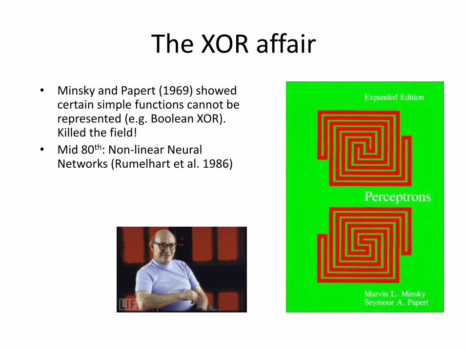
The XOR affair

• Minsky and Papert (1969) showed certain simple functions cannot be represented (e.g. Boolean XOR). Killed the field!

• Mid 80th: Non-linear Neural Networks (Rumelhart et al. 1986)

The XOR affair

Neural Networks

• Rich history, starting in the early forties (McCulloch and Pitts 1943).

• Two views: – Modeling the brain

– “Just” representation of complex functions (Continuous; contrast decision trees)

• Much progress on both fronts.

• Drawn interest from: Neuroscience, Cognitive science, AI, Physics, Statistics, and CS/EE.

Neuron

Neural Structure

1. Cell body; one axon (delivers output to other connect neurons); many dendrites (provide surface area for connections from other neurons).

2. Axon is a single long fiber. 100 or more times the diameter of cell body. Axon connects via synapses to dendrites of other cells.

3. Signals propagated via complicated electrochemical reaction.

4. Each neuron is a “threshold unit”. Neurons do nothing unless the collective influence from all inputs reaches a threshold level.

5. Produces full-strength output. “fires”. Stimulation at some synapses encourages neurons to fire; some discourage from firing.

6. Synapses can increase (excitatory) or decrease (inhibitory) potential (signal

Why Neural Nets?

Motivation:

Solving problems under the constraints similar to those of the brain may lead to solutions to AI problems that would otherwise be overlooked.

• Individual neurons operate very slowly But the brain does complex tasks fast: massively parallel algorithms

• Neurons are failure-prone devices But brain is reliable anyway distributed representations

• Neurons promote approximate matching less brittle learnable

Connectionist Models of Learning

Characterized by:

• A large number of very simple neuron-like processing elements.

• A large number of weighted connections between the elements.

• Highly parallel, distributed control.

• An emphasis on learning internal representations automatically.

Artificial Neurons

Activation Functions:

stept (x) = 1, if x ≥ t; otherwise 0. sign(x) = +1, if x ≥ 0; otherwise -1 sigmoid(x) = 1/(1+e-x)

Example: Perceptron

Perceptrons Single Layer Feed Forward Neural Networks

Can be easily trained using perceptron algorithm

2-Layer Feedforward Networks Boolean functions:

• Every boolean function can be represented by network with single hidden layer

• But might require exponential (in number of inputs) hidden units

Continuous functions:

• Every bounded continuous function can be approximated with arbitrarily small error, by network with one hidden layer [Cybenko 1989; Hornik et al. 1989]

Any function can be approximated to arbitrary accuracy by a network with two hidden layers [Cybenko 1988].

x1

x2

xN

o1

o2

oO

Multi-Layer Nets

• Fully connected, two layer, feedforward

Jonathan

Mary

Joe

Elizabeth

Alice

Bart How are Mary and Elizabeth related? A=Acquaintances B=Family

Activation function: g(x) = (1 if greater than threshold, 0 otherwise)

Multi-Layer Nets

• Fully connected, two layer, feedforward

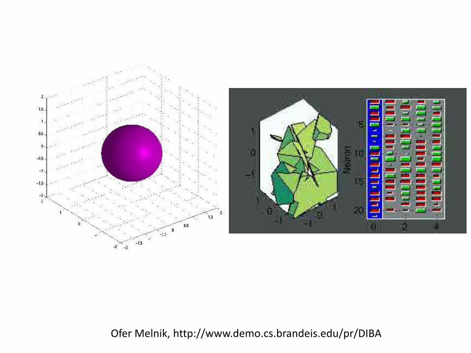
Ofer Melnik, http://www.demo.cs.brandeis.edu/pr/DIBA

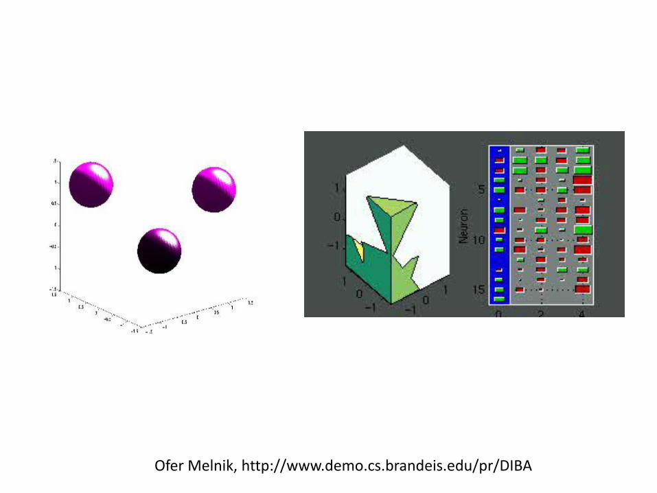
Ofer Melnik, http://www.demo.cs.brandeis.edu/pr/DIBA

Ofer Melnik, http://www.demo.cs.brandeis.edu/pr/DIBA

How can we train perceptrons?

Hebbian learning

• D. O. Hebb: – The general idea is an old one, that any two cells or systems of

cells that are repeatedly active at the same time will tend to become 'associated', so that activity in one facilitates activity in the other." (Hebb 1949, p. 70)

– "When one cell repeatedly assists in firing another, the axon of the first cell develops synaptic knobs (or enlarges them if they already exist) in contact with the soma of the second cell." (Hebb 1949, p. 63)

• Cells that fire together, wire together – If error is small, increase magnitude of connections that

contributed. – If error is large, decrease magnitude of connections that

contributed.

Backpropagation

• Classical measure of error – Sum of square errors

– hw(x) is output on perceptron on x.

• Gradient decent using partial derivatives

• Update weights

Backpropagation Training (Overview) Training data:

– (x1,y1),…, (xn,yn), with target labels yz {0,1}

Optimization Problem (single output neuron): – Variables: network weights wij

– Obj.:E=minw∑z=1..n(yz–o(xz))2,

– Constraints: none

Algorithm: local search via gradient descent. • Randomly initialize weights. • Until performance is satisfactory,

– Compute partial derivatives ( E / wi j) of objective function E for each weight wi j

– Update each weight by wi j à wi j + ( E / wi j)

Smooth and Differentiable Threshold Function

• Replace sign function by a differentiable activation function sigmoid function:

Slope of Sigmoid Function

Backpropagation Training (Detail)

• Input: training data (x1,y1),…, (xn,yn), learning rate parameter α. • Initialize weights. • Until performance is satisfactory

– For each training instance, • Compute the resulting output

• Compute βz = (yz – oz) for nodes in the output layer

• Compute βj = ∑k wjk ok (1 – ok) βk for all other nodes.

• Compute weight changes for all weights using

∆wi j(l) = oi oj (1 – oj) βj

– Add up weight changes for all training instances, and update the weights accordingly. wi,j ← wi,j + α ∑l ∆wi,j(l)

Summary: Hidden Units

• Hidden units are nodes that are situated between the input nodes and the output nodes.

• Hidden units allow a network to learn non-linear functions.

• Hidden units allow the network to represent combinations of the input features.

• Given too many hidden units, a neural net will simply memorize the input patterns (overfitting).

• Given too few hidden units, the network may not be able to represent all of the necessary generalizations (underfitting).

How long should you train the net?

When would you stop training?

A B C D E

How long should you train the net?

• The goal is to achieve a balance between correct responses for the training patterns and correct responses for new patterns.

– That is, a balance between memorization and generalization)

• If you train the net for too long, then you run the risk of overfitting.

– Select number of training iterations via cross-validation on a holdout set.

Regularization

• Simpler models are better

• NN with smaller/fewer weights are better

– Add penalty to total sum of absolute weights

– Pareto optimize

Design Decisions

• Choice of learning rate

• Stopping criterion – when should training stop?

• Network architecture

– How many hidden layers? How many hidden units per layer?

– How should the units be connected? (Fully? Partial? Use domain knowledge?)

• How many restarts (local optima) of search to find good optimum of objective function?

Spiking Nets

• Represent continues values using rates

– Output spike if # of incoming spikes > threshold

– Leaky counter

http://www.ine-news.org

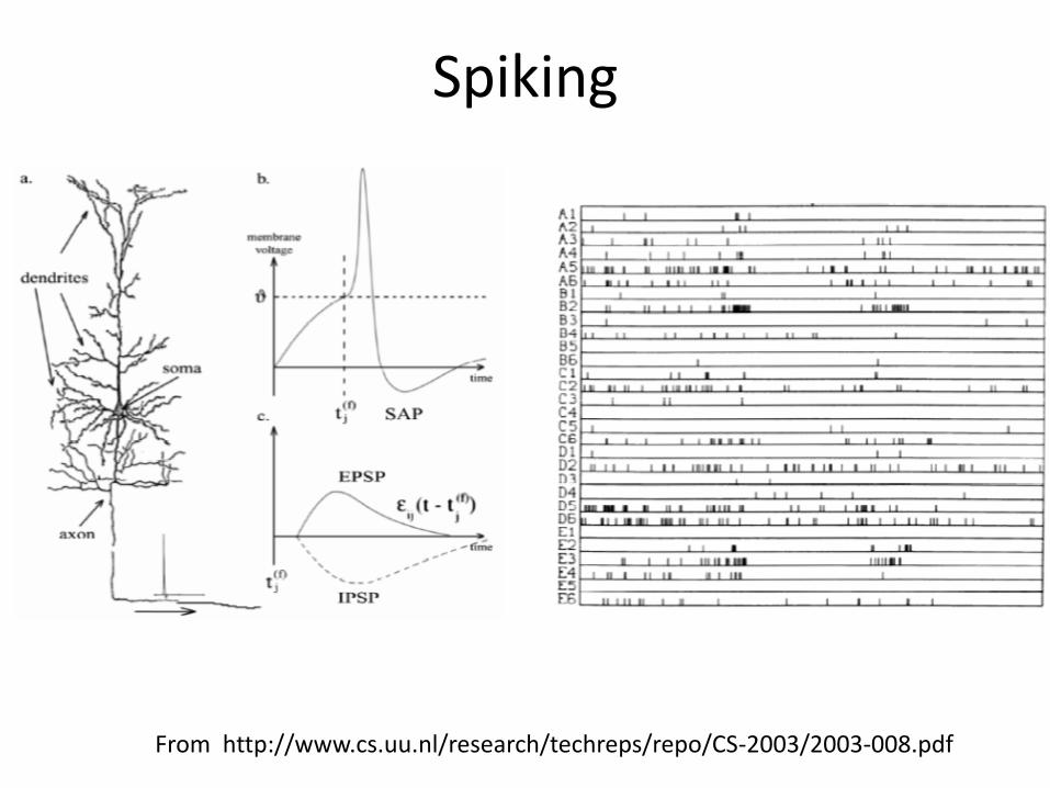
From http://www.cs.uu.nl/research/techreps/repo/CS-2003/2003-008.pdf

Spiking

Recurrent networks

• Nodes connect

– Laterally

– Backwards,

– To themselves

• Complex behavior

– Dynamics, Memory

www.stowa-nn.ihe.nl/ANN.htm

Learning Network Topology

• Optimal Brain Damage algorithm – Trains a fully connected network – Removes connections and nodes that contribute least

to the performance • Using information-theoretic criteria

– Repeats until performance starts decreasing

• Tiling algorithm: Grows networks – Start with a small network that classifies many

examples – Repeatedly add more nodes to classify remaining

examples

Hyper-Networks

• Use a network to generate a network

– E.g. to determine connection wij use network that takes in i and j and produces w.

– In 2D:

Ken Stanley, eplex.cs.ucf.edu

Hyper-Networks

Ken Stanley, eplex.cs.ucf.edu