artificial neural networksncd.sy/upload/projects/project_file_396.pdf · jeopardy champions by a...

Jaber Adeeb | Informatics | 2015-2016

Artificial Neural Networks A MODELED BRAIN

Contents

Preface .......................................................................................................................... 1

Chapter 1

Introduction and history .......................................................................................... 2

1.1 A brief history .................................................................................................. 2

1.2 An introduction to neural networks .............................................................. 4

1.3 A simple example ............................................................................................ 6

1.4 The way of learning in a simple description .................................................. 7

Chapter 2

A deeper glance .......................................................................................................... 8

Biological hints first ........................................................................................ 8

The modelling process ................................................................................... 11

2.2.1 Basic concepts and definitions .................................................................... 11

2.2.2 Network topologies .................................................................................... 14

2.2.3 Paradigms of learning ................................................................................. 15

An artificial life maybe?! .......................................................................................... 17

References .................................................................................................................. 19

Preface

Artificial Intelligence known as AI was officially founded at a conference on Dartmouth College’s campus in 1956. The conference included John McCarthy, Marvin Minsky, Allen Newell, Arthur Samuel and Herbert Simon, who became the leaders of AI research for many decades.

AI spread broadly since 1960 and was heavily funded in different countries. During its evolving, AI showed in many forms, some were linked to each other and some were independent branches of it. In the 1980s one of AI’s first successful forms emerged, expert systems, which are computer systems that emulate the decision making ability of a human expert to solve complex problems for example.

In the 1990s and early 21st century AI reached a great level of success due to several factors: the increasing computational power of computers, a greater emphasis on solving specific sub problems, the creation of new ties between AI and other fields working on similar problems and a new commitment by researchers to solid mathematical methods and rigorous scientific standards.

Throughout its success AI fulfilled a lot of achievements, such as: deep blue, the chess playing computer which beaten Garry Kasparov, a reigning world chess champion. IBM’s question answering system, Watson, defeated two of the best jeopardy champions by a significant margin in a Jeopardy! quiz show. A 3D body-motion interface provider became available for the Xbox 360 and the Xbox One, the Kinect. A lot more became available.

AI provided a lot of products and creations that implemented reasoning, problem solving capability, knowledge, planning, learning, communication, perception and more.

One of AI’s applications was Artificial Neural Networks which is a simulation of a biological humanoid neural network or in other words a simulation of a humanoid brain, so it’s able to learn, to solve mathematical or complex problems by itself starting from simpler ones and to make use the capabilities of its artificial components to the maximum.

What are the advantages and disadvantages of an artificial neural network??

Could we keep track on its every action and keep it under control??

Before answering these questions let’s take a deep look into artificial neural networks and their specifications.

Chapter 1

Introduction and history

1.1 A BRIEF HISTORY

Instead of a long historical talk, I decided to build a timeline with multiple dates of interest containing brief information about important achievements or events that happened in them.

It started in the early 1940s and went on as the following:

1943: models of neurologial networks were intrduced by Warren

McCulloch and Walter Pitts, these networks were able to calculate almost any logic or arithmetic function. The first computer precursors (“electronic brains”) were developped.

1947: McCulloch and Pitts indicated a practical field of application which

was not mentioned in their work from 1943 (the recognition of special patterns).

1949: the classical Hebbian rule was formulated by Donald O. Hebb which

in its generalized form represents nearly all neural learning procedures.

1950: the neuropsychologist Karl Lashley defended the thesis that brain

information storage is realized as a distributed system (the extent of a destroyed nerve tissue is affected and not its location).

1951: from this year and so on, neural networks field reached its golden age.

Marvin Minsky developed the neurocomputer Snark which was capable of calculating and adjusting its weights automatically.

1956: some well-known scientists and ambitious students met at the

Dartmouth Summer Research Project and discussed, if right to say, how to simulate a brain and the differences between top-down and bottom-up research. Supporters of neural networks wanted to achieve a simulation of the smallest part of a biological neural system – the neurons.

1957-1958: the neurocomputer Mark I perceptron was developed by Frank

Rosenblatt, Charles Wightman and their coworkers at the MIT.

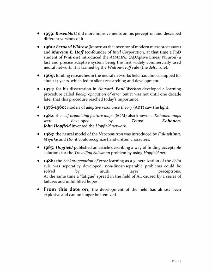
1959: Rosenblatt did more improvements on his perceptron and described

different versions of it.

1960: Bernard Widrow (known as the inventor of modern microprocessors)

and Marcian E. Hoff (co-founder of Intel Corporation, at that time a PhD student of Widrow) introduced the ADALINE (ADAptive LInear NEuron) a fast and precise adaptive system being the first widely commercially used neural network. It is trained by the Widrow-Hoff rule (the delta rule).

1969: funding researches in the neural networks field has almost stopped for

about 15 years, which led to silent researching and development.

1974: for his dissertation in Harvard, Paul Werbos developed a learning

procedure called Backpropagation of error but it was not until one decade later that this procedure reached today’s importance.

1976-1980: models of adaptive resonance theory (ART) saw the light.

1982: the self-organizing feature maps (SOM) also known as Kohonen maps

were developed by Teuvo Kohonen. John Hopfield invented the Hopfield network.

1983: the neural model of the Neocognitron was introduced by Fukushima,

Miyake and Ito, it couldrecognize handwritten characters.

1985: Hopfield published an article describing a way of finding acceptable

solutions for the Travelling Salesman problem by using Hopfield net.

1986: the backpropagation of error learning as a generalization of the delta

rule was seperatley developed, non-linear-separable problems could be solved by multi layer perceptrons. At the same time a “fatigue” spread in the field of AI, caused by a series of failures and unfullfilled hopes.

From this date on, the development of the field has almost been

explosive and can no longer be itemized.

1.2 AN INTRODUCTION TO NEURAL NETWORKS

If we want to solve a problem using a machine, we could simply formulate it as an algorithm, but there are many problems that cannot be formulated this way, still, our human brain is able to solve them, why is that so?

It’s because we, unlike machines, learn.

Computers have some processing units and memory which makes them able of doing complex numerical calculations in a very short time, but these components are not adaptive.

Theoretically, if we compare a human brain to a computer, we will see that a computer should be more powerful than our brain: it comprises 109 transistors with a switching time of 10-9 while the brain contains 1011 neurons with a switching time of about 10-8.

A simple comparison might explain better:

BRAIN COMPUTER

No. of processing units ≈ 1011 ≈ 109

Type of processing units Neurons Transistors

Type of calculation Massively parallel Usually serial

Data storage Associative Address-based

Switching time ≈ 10-8 s ≈ 10-9 s

Possible switching operations ≈ 1013 s-1 ≈ 1018 s-1

Actual switching operations ≈ 1012 s-1 ≈ 1010 s-1

Table 1: a simple comparison between a human brain and a computer.

The brain, being parallel, is working to its theoretical maximum, from which the computer is orders of magnitude away. A computer is also static – the brain, as a biological neural network can reorganize itself during its “lifespan” and therefore is able to learn, to compensate errors and so forth.

The study of artificial neural networks is motivated by their similarity to successfully working biological systems, which consist of simple but numerous nerve cells that work massively in parallel and have the capability to learn (which is one of its most significant aspects).

There is no need to explicitly program a neural network. For instance it can learn from training samples or by means of encouragement (reinforcement learning.)

This learning technique leads to a neural network that’s capable of generalizing and associating data, because after a successful training a neural network could be able to find reasonable solutions to similar problems of the same class that were not explicitly trained. This results in a high degree of fault tolerance against noisy input data.

Fault tolerance is strongly related to biological neural networks in which this characteristic is very distinct: neurons reorganize themselves or are reorganized by external influences. Although this happens or cognitive abilities are not significantly affected. Thus the brain (or the biological neural network) is tolerant against internal and external errors, for we can often read some “dreadful scrawls” although the individual letters are barely readable.

If we observe our modern technology, then we can easily notice that it’s not automatically fault-tolerant. There’s never been a machine that could overcome missing a hardware piece, imagine if there’s a laptop without a hard disk controller, the audio card would never take over its tasks. So when something is damaged in a machine, it’s affected as a whole, while a brain is not.

At first sight, this distributed system seems pretty adequate and efficient, but no system is flawless, a disadvantage of this system is the difficulty of analyzing the neural network at first sight (we can’t tell what it knows nor what it does nor where its faults lie). Most often we can only transfer knowledge into the network by means of a learning procedure, which, besides being hard to manage, might cause errors.

So to create an artificial neural network which implements a biological one, we need to adapt four basic characteristics:

Self-organization.

Learning capabilities.

Generalization capability.

Fault tolerance.

1.3 A SIMPLE EXAMPLE

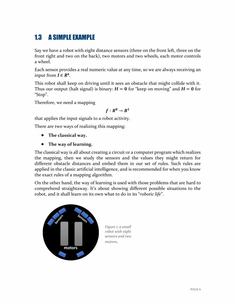
Say we have a robot with eight distance sensors (three on the front left, three on the front right and two on the back), two motors and two wheels, each motor controls a wheel.

Each sensor provides a real numeric value at any time, so we are always receiving an input from I ∈ R8.

This robot shall keep on driving until it sees an obstacle that might collide with it. Thus our output (halt signal) is binary: H = 𝟎 for “keep on moving” and H = 𝟎 for “Stop”.

Therefore, we need a mapping

𝒇 ∶ 𝑹𝟖 → 𝑩𝟏

that applies the input signals to a robot activity.

There are two ways of realizing this mapping:

The classical way.

The way of learning.

The classical way is all about creating a circuit or a computer program which realizes the mapping, then we study the sensors and the values they might return for different obstacle distances and embed them in our set of rules. Such rules are applied in the classic artificial intelligence, and is recommended for when you know the exact rules of a mapping algorithm.

On the other hand, the way of learning is used with those problems that are hard to comprehend straightaway. It’s about showing different possible situations to the robot, and it shall learn on its own what to do in its “robotic life”.

Figure 1: a small robot with eight sensors and two

motors.

1.4 THE WAY OF LEARNING IN A SIMPLE DESCRIPTION

To teach a “neural network” we first treat it as a “black box” (we don’t know its structure but just regard its behavior in practice).

We introduce the robot to its first training samples, which are situations in form of simply measured sensor values, we specify whether the robot shall drive on or stop. Thus a training sample consists of an exemplary input and a corresponding desired output. So how do we transfer this knowledge and the information into the neural network?!

We can teach the samples to a neural network by using a simple learning procedure, which is a simple algorithm or a mathematical formula. If we have done everything right and chosen good samples, the neural network will generalize from these samples and find a universal rule when it has to stop.

The aforementioned example can be optionally expanded for the purpose of direction control for example, it would be possible to control the two motors of the robot separately, with the sensor layout unchanged. But in this case we are looking for a mapping

𝒇 ∶ 𝑹𝟖 → 𝑹𝟐

which gradually control the two motors by means of the sensor inputs and thus cannot only, for example, stop the robot but also lets it avoid obstacles. It has become more difficult to analytically derive the rules, and de facto a neural network would be more appropriate.

The goal here is not to learn the samples by heart but to understand the principle behind them: Ideally, the robot should apply the neural network in any situation and be able to avoid obstacles. So the robot should continuously and repeatedly query the network while driving in order to continuously avoid obstacles. This results in a constant cycle: the robot queries the network, it will drive in one direction as a consequence, which changes the sensors values. Again the robot queries the network and changes its position, the sensors values are changed once again, and so on. It is obvious that this system can also be adapted to dynamic (changing environments, moving obstacles in our example…).

Figure 2: different positions with different sensor values as learning samples.

Figure 3: neuron's components.Figure 4: different positions with different sensor values as learning

samples.

Chapter 2

A deeper glance

BIOLOGICAL HINTS FIRST

Before going any deeper into the artificial neural networks, we should have some basic information of biological ones, which we will briefly discuss in this part.

Information gets processed by the vertebrate nervous system, which consists of the central nervous system and the peripheral nervous system.

The peripheral nervous system comprises the nerves that are situated outside the brain or the spinal cord. These nerves form a branched and very dense network throughout the whole body.

The central nervous system, however is the “main frame”. It’s the management and storing part for all the information received by the sense organs besides controlling the inner processes in the body and last but not least, coordinates the motor functions of the organism.

The cerebrum is one of the most important part of the nervous system, it changed most during evolution. It is responsible for a lot of operations much of them is controlled consciously by the being (such as decision making, problem solving, purposeful behaviors, consciousness, emotions, voluntary movements…).

The cerebellum is located below the cerebrum and is in charge of performing motor coordination, maintaining balance, controlling movements and continuously correcting errors. For this purpose, the cerebellum has direct sensory information about muscle lengths as well as acoustic and visual information. Furthermore, it also receives messages about more abstract motor signals coming from the cerebrum.

The diencephalon (the interbrain) includes the thalamus, which mediates between sensory and motor signals and the cerebrum. Particularly it decides which part of the information is transferred to the cerebrum, so that especially less important sensory perceptions can be suppressed at short notice to avoid overloads. Another part of the diencephalon is the hypothalamus, which controls a number of processes within the body. The diencephalon in the human circadian rhythm (“internal clock”) and the sensation of pain.

One last component is the brainstem, which connects the brain with the spinal cord and is responsible for many fundamental reflexes, such as the blinking reflex or coughing.

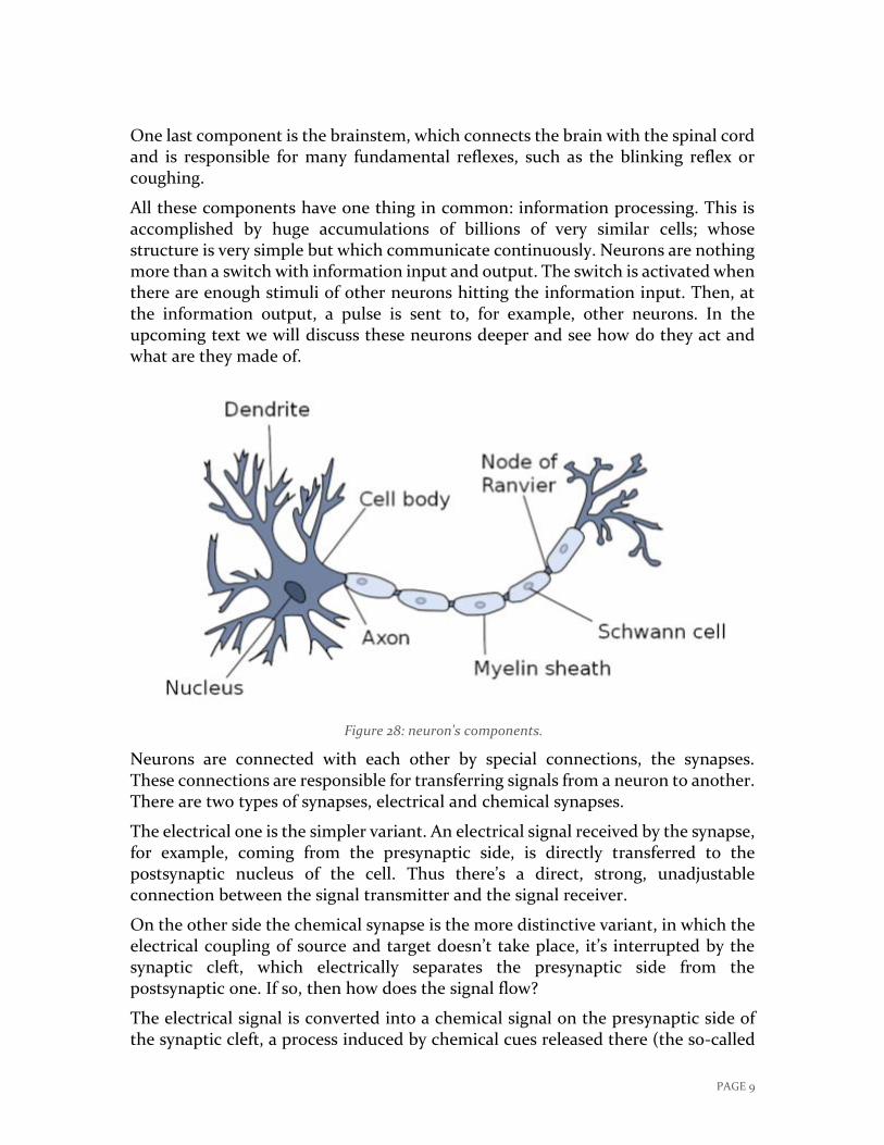
All these components have one thing in common: information processing. This is accomplished by huge accumulations of billions of very similar cells; whose structure is very simple but which communicate continuously. Neurons are nothing more than a switch with information input and output. The switch is activated when there are enough stimuli of other neurons hitting the information input. Then, at the information output, a pulse is sent to, for example, other neurons. In the upcoming text we will discuss these neurons deeper and see how do they act and what are they made of.

Neurons are connected with each other by special connections, the synapses. These connections are responsible for transferring signals from a neuron to another. There are two types of synapses, electrical and chemical synapses.

The electrical one is the simpler variant. An electrical signal received by the synapse, for example, coming from the presynaptic side, is directly transferred to the postsynaptic nucleus of the cell. Thus there’s a direct, strong, unadjustable connection between the signal transmitter and the signal receiver.

On the other side the chemical synapse is the more distinctive variant, in which the electrical coupling of source and target doesn’t take place, it’s interrupted by the synaptic cleft, which electrically separates the presynaptic side from the postsynaptic one. If so, then how does the signal flow?

The electrical signal is converted into a chemical signal on the presynaptic side of the synaptic cleft, a process induced by chemical cues released there (the so-called

Figure 28: neuron's components.

neurotransmitters). These neurotransmitters cross the synaptic cleft and transfer the information into the nucleus of the cell, where it is reconverted into the electrical information.

Although they are complex, the chemical synapses have – compared with the electrical synapses – utmost advantage:

One-way connection.

Adjustability.

Briefly, the signal is processed this way:

Dendrites receive (collect) all part of information (many electrical signals from many sources), then they are processed (accumulated) in the soma and if it exceeds a certain value (threshold value), it’s transferred to the next neuron. Outgoing pulses are transferred by means of the axon.

As we have seen, information is processed on every level of the nervous system, and then, a proper response happens.

Now that we have a brief knowledge of how a biological neural network works, we can move onto the next part, which is modelling this biological network into an artificial one.

THE MODELLING PROCESS

2.2.1 Basic concepts and definitions

To make an artificial model of a neural network, we need to implement a few elements which are:

Vectorial input: the input of technical neurons should consist of many components; therefore, it is a vector. In nature a neuron receives pulses of 103 to 104 other neurons on average.

Scalar output: the output of a neuron is a scalar (one component), so several scalar outputs form the vectorial input of another neuron. This also means that various input components have to be summarized somehow so that one component remains.

Synapses change input: the inputs in a neural network – both biological original and technical adaptation – are weighted, which means they are multiplied by a number called weight, so they are preprocessed, if right to say.

Accumulating the inputs: biologically, inputs are summarized into a pulse, while on the technical side this is often realized by the weighted sum. This means that after accumulation we continue with one value, a scalar, instead of a vector.

Non-linear characteristic: the input of a technical neuron is not proportional to the output.

Adjustable weights: the weights weighing the inputs are variable, similar to the chemical process at the synaptic cleft, which adds a great dynamic to the network.

After mentioning these characteristics, we could conclude some simple basic specifications of a casually formulated and very simple neuron model:

It receives a vectorial input

with components 𝒙𝒊. These are multiplied by the appropriate weights 𝒘𝒊 and accumulated:

∑𝒘𝒊𝒙𝒊

𝒊

This term is called weighted sum. Then the non-linear mapping 𝒇 defines the scalar output 𝒚:

𝒚 = 𝒇(∑𝒘𝒊𝒙𝒊

𝒊

)

Time as a concept will be divided to discrete time steps (present time is (𝒕) and the next time step is (𝒕 + 𝟏) and the previous is (𝒕 − 𝟏) and anything related to time is written this way (𝑶𝒊(𝒕)). These are the basic things we need to know before knowing

the components of a technical neural network.

A technical neural network is consisted of simple processing units, neurons, and directed, weighted connections between those neurons. The strength of a connection (the connecting weight) between two neurons 𝒊 and 𝒋 is referred to as 𝒘𝒊𝒋.

A neural network is a sorted triple (𝑵, 𝑽,𝒘) with two sets 𝑵, 𝑽 and a function 𝒘, where 𝑵 is the set of neurons and 𝑽 a set (𝒊, 𝒋) | 𝒊, 𝒋 ∈ ℕ whose elements are called connections between neuron 𝒊 and neuron 𝒋. The function 𝒘 ∶ 𝑽 → ℝ defines the

weights, where 𝒘((𝒊, 𝒋)), the weight of the connection between neuron 𝒊 and neuron

𝒋, is shortened to 𝒘𝒊𝒋. Depending on the point of view it is either 0 for connections

that do not exist in the network.

So the weights can be implemented in a square weight matrix 𝑾 or, optionally, in a weight vector 𝑾 with the row number of the matrix indicating where the connection begins, and the column number of the matrix indicating, which neuron is the target. This matrix representation is also called Hinton diagram.

Data are transferred between neurons via connections with the connecting weight being either excitatory or inhibitory.

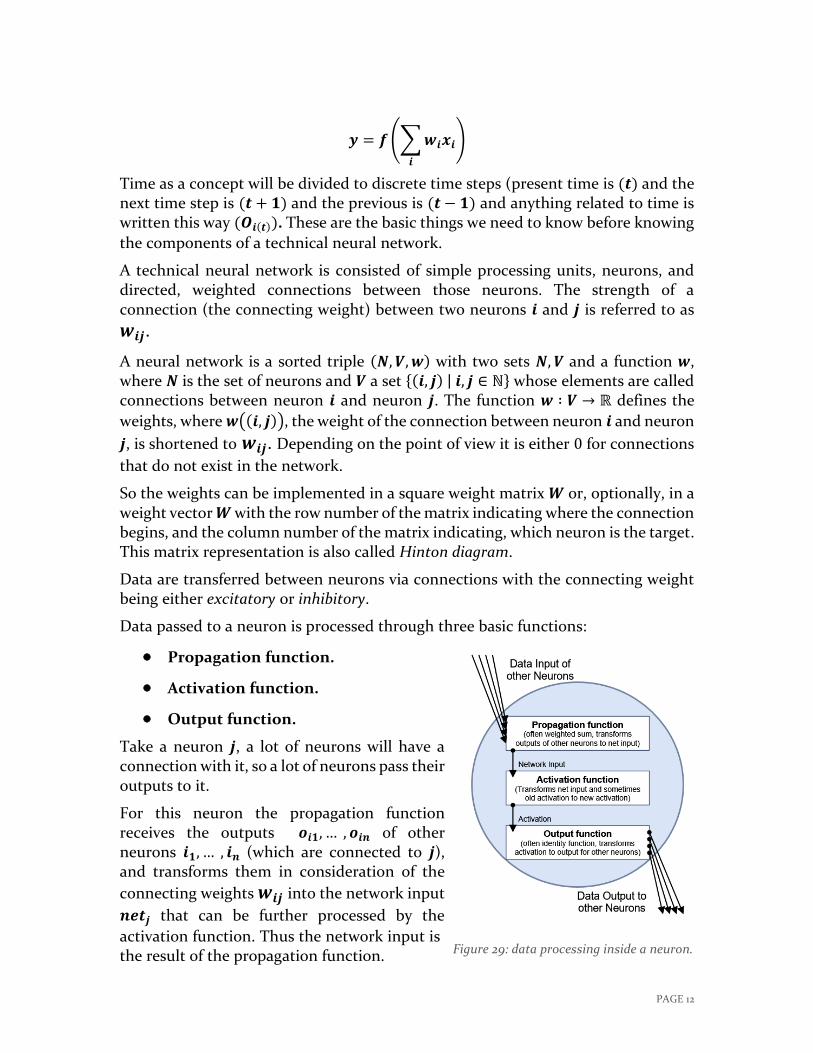
Data passed to a neuron is processed through three basic functions:

Propagation function.

Activation function.

Output function.

Take a neuron 𝒋, a lot of neurons will have a connection with it, so a lot of neurons pass their outputs to it.

For this neuron the propagation function receives the outputs 𝒐𝒊𝟏, … , 𝒐𝒊𝒏 of other neurons 𝒊𝟏, … , 𝒊𝒏 (which are connected to 𝒋), and transforms them in consideration of the

connecting weights 𝒘𝒊𝒋 into the network input

𝒏𝒆𝒕𝒋 that can be further processed by the

activation function. Thus the network input is the result of the propagation function. Figure 29: data processing inside a neuron.

Let’s define the propagation function and the network input

let 𝑰 = 𝒊𝟏, 𝒊𝟐, … , 𝒊𝒏 be the set of neurons, such that ∀ 𝒛 ∈ 𝟏,… , 𝒏 ∶ ∃ 𝒘𝒊𝒛𝒋.

Then the network input of 𝒋, called 𝒏𝒆𝒕𝒋, is calculated by the propagation function

𝒇𝒑𝒓𝒐𝒑 as follows:

𝒏𝒆𝒕𝒋 = 𝒇𝒑𝒓𝒐𝒑((𝒐𝒊𝟏 , … , 𝒐𝒊𝒏), (𝒘𝒊𝟏𝒋, … , 𝒘𝒊𝒏𝒋))

Here the weighted sum is very popular: the multiplication of the output of each neuron 𝒊 by 𝒘𝒊𝟏𝒋, and the summation of the results:

𝒏𝒆𝒕𝒋 = ∑(𝒐𝒊. 𝒘𝒊𝟏𝒋)

𝒊∈𝑰

Every neuron is, to a certain extent, at all times active (excited). the activation state 𝒂𝒋 of a neuron indicates the extent of its activation and is often

shortly referred to as activation.

Neurons are activated if their network input exceeds their threshold value 𝜽𝒋, which

is a value a neuron starts firing when exceeded.

The activation function (sometimes referred to as transfer function) determines the activation of a neuron dependent on network input, previous activation state and threshold value as follows:

𝒂𝒋(𝒕) = 𝒇𝒂𝒄𝒕(𝒏𝒆𝒕𝒋(𝒕), 𝒂𝒋(𝒕 − 𝟏), 𝜽𝒋)

There are many variants to the activation function:

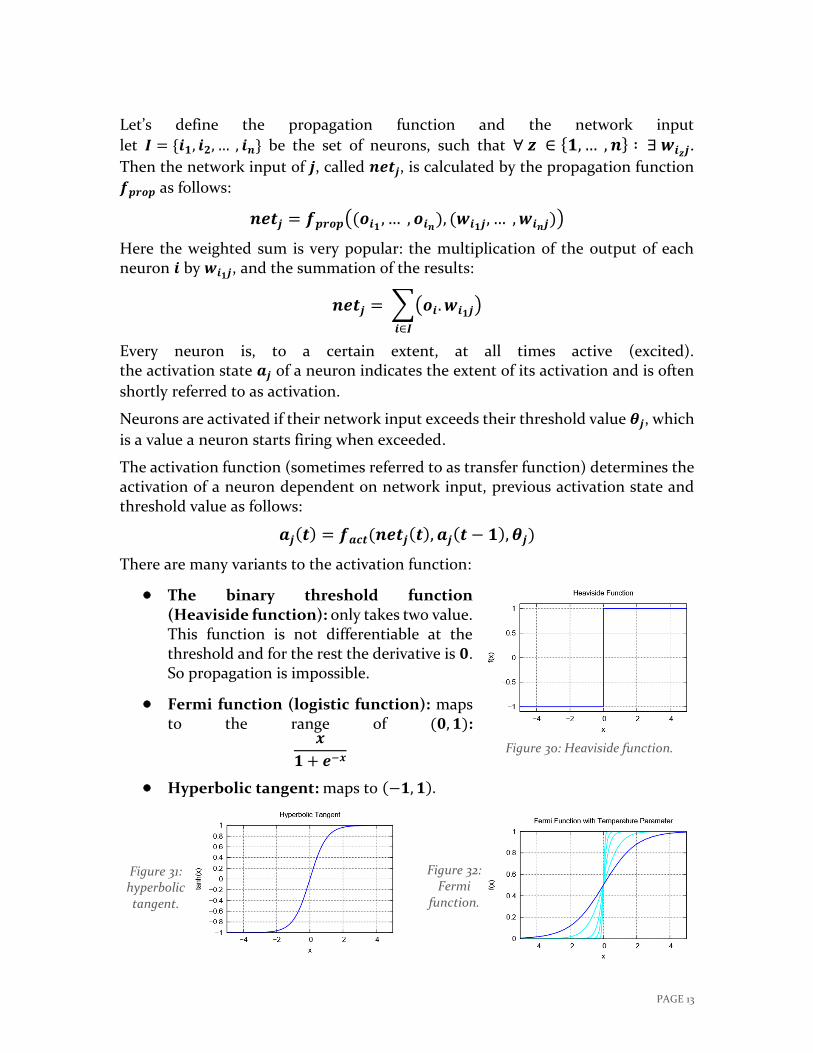
The binary threshold function (Heaviside function): only takes two value. This function is not differentiable at the threshold and for the rest the derivative is 𝟎. So propagation is impossible.

Fermi function (logistic function): maps to the range of (𝟎, 𝟏):

𝒙

𝟏 + 𝒆−𝒙

Hyperbolic tangent: maps to (−𝟏, 𝟏).

Figure 30: Heaviside function.

Figure 32: Fermi

function.

Figure 31: hyperbolic tangent.

The hyperbolic tangent was replaced with two parabola pieces and two half-lines, which made the calculations up to 200 times faster at the price of a slightly smaller range of values than the hyperbolic tangent ([−𝟎. 𝟗𝟔𝟎𝟏𝟔, 𝟎. 𝟗𝟔𝟎𝟏𝟔] instead of [−𝟏, 𝟏]).

The output function calculates the output value of a neuron from its activation state:

𝒇𝒐𝒖𝒕(𝒂𝒋) = 𝒐𝒋

this function is often the identity, i.e. the activation 𝒂𝒋 is directly output:

𝒇𝒐𝒖𝒕(𝒂𝒋) = 𝒂𝒋, so 𝒐𝒋 = 𝒂𝒋

Both the activation and the output functions are often set globally.

All these components and functions are organized or adjusted by a so called learning strategy, which is an algorithm used to change and thereby train the neural network so that the neural network produces a desired output for a given input.

2.2.2 Network topologies

It’s now time to get familiar with the usual topologies (designs) of neural networks.

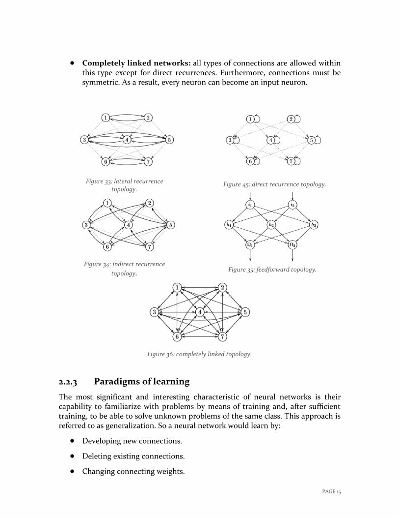
Feedforward networks: in this type the neurons are grouped into three sections: input layer, hidden layers, output layer (we, from now on, will refer to output neurons with Ω. Each neuron within a feedforward network has only directed connections to the neurons of the next layer, and so on towards the output layer. There are some cases, in which, a neuron could skip connecting to one or more layers and connect to any other subsequent layer as long as the connection is directed towards the output layer.

Recurrent networks: these networks have influence on themselves (a neuron influences itself by any means or connection). These networks do not have explicitly defined input or output neurons. within some of these networks neurons are allowed to connect to themselves directly, in which case, they are called direct recurrent networks. neurons within direct recurrent networks inhibit and strengthen themselves to reach their activation limits in the process. another type is the indirect recurrent networks, in which, a neuron can connect to the preceding layer. The last recurrent type is the lateral recurrent network which allows connections between neurons of the same layer, so each neuron often inhibits the other neurons of the layer and strengthens itself. As a result, the strongest neuron becomes active, so, if right to say, it’s a winner-take-all scheme.

Completely linked networks: all types of connections are allowed within this type except for direct recurrences. Furthermore, connections must be symmetric. As a result, every neuron can become an input neuron.

2.2.3 Paradigms of learning

The most significant and interesting characteristic of neural networks is their capability to familiarize with problems by means of training and, after sufficient training, to be able to solve unknown problems of the same class. This approach is referred to as generalization. So a neural network would learn by:

Developing new connections.

Deleting existing connections.

Changing connecting weights.

Figure 35: feedforward topology.

Figure 45: direct recurrence topology.

Figure 34: indirect recurrence

topology.

Figure 33: lateral recurrence topology.

Figure 36: completely linked topology.

Changing the threshold values of neurons.

Varying one or more of the three neuron functions (activation, propagation, and output functions).

Developing new neurons.

Deleting existing neurons, which is accompanied by deleting existing connections.

We direct the learning of a neural network by a, so called, learning procedure, which is a set of rules formulated as an algorithm that can easily be implemented by means of a programming language.

There are three main and essential paradigms (unsupervised, reinforcement and supervised learning), and they shall be introduced by presenting the differences between their regarding training sets.

Unsupervised learning is the most plausible method, biologically speaking, but is not suitable for all problems. Its training set only consist of input patterns, and the network tries by itself to detect similarities and to generate pattern classes.

In reinforcement learning, the training set consists of input patterns, and after completing a sequence, a value is returned to the network indicating whether the result was right or wrong and possibly, how right or wrong it was (the stick and carrot policy).

Supervised learning is an extremely effective, and therefore very practicable, learning procedure, in which the training set consists of input patterns with their corresponding correct results, so that the network can receive a precise error vector. This procedure goes like this:

Entering the input pattern (activation of input neurons).

Forward propagation of the input by the network, output is generated.

Comparing the output with the desired output (teaching input).

Providing the error vector (difference vector).

Corrections of the network are calculated based on the error vector.

Corrections are applied.

There are two main ways of learning, online and offline leaning. Using online learning the network learns directly from the errors of each training sample, while using offline learning, the network receives several training patterns and the errors care accumulated, here, the network learns for all patterns at the same time.

An artificial life maybe?!

Artificial neural networks could be of benefit almost everywhere, because of their adaptive design, their characteristics and their ability to learn. But the question to be asked is will these networks ever be able to reach the “intelligence” level of our human brain?!

To answer this question, we first need to know the difference between our brain and these network’s regarding the tasks they can do.

Our brain is capable of learning, extremely faster than an artificial neural network does, it’s capable of doing a whole bunch of tasks and operations all together at the same time, but we as humans do not give them that important notice, for they are everyday tasks so we view them as ordinary tasks and operations, some examples might speak clearer.

If you show a flower to a kid, who has never seen one, and tell him it’s a flower, flip it upside down for example and ask him what does he see, what would his answer be? It will definitely be a flower, on the other hand, do the same with an artificial neural network, the flower has been saved to its memory as in the first position, when flipped, it is no more a flower to the network, it is nothing recognizable yet (it has to see a flower in a lot of positions and a lot of conditions before having the ability to “know” what a flower is).

Our brain has a really high level of multitasking, it does a great number of tasks simultaneously, more than any computer or technical hardware or software was ever able to, it organizes breathing, heart beating rate, blood pressure, all five senses are always activated unless one of their organs is corrupted, so we see and listen and smell and taste and touch at the same instance. Our simple movements are more complicated than you think it is, for example it takes a good amount of time to make a robotic hand that has the same ability to as a humanoid one.

What we do in our everyday life is much more complicated than we could imagine and it is tremendously hard for a computer or an artificial neural network to do. Our brain is able to recognize stuff only after seeing them one time, it is able to differentiate between similar stuff easily, it is able to multitask more than any artificial component.

Artificial neural networks on the other side, could be able to do some of these tasks, but takes much more time to learn them. They are able to predict futuristic results based on present and past data, they are able to complete really complex calculations and computations within seconds, they are able to recognize handwritten characters and words in bad conditions, recognize styles in paintings, novels and poems or even mathematical sheets, and after sufficient learning amount, they could output other products of the same class with the same style or

be given, for example, a document with totally scrambled characters, and return a totally readable one with a specific style.

Artificial neural networks could even learn to master some task, a game for example, starting from scratch within a reasonable time.

Until now, most of the AI related products, including artificial neural networks, deliver a massively accurate and efficient experience considering a single or a couple of operations no more, never a fully functional product that could “understand” but one that “knows” and judges based on its knowledge alone, so will we ever be able to create a product that could replace a human at an important position, or to be able to invent something at its own level or more advanced, or to duplicate itself and organize its “clones”.

These questions will be left unanswered for a good while, and we have not even get close enough to answer or achieve some of them.

But the evolution technology had seen during the last decades stands proof that everything is possible given enough time, so nobody knows when these achievements will be reached.

In my opinion, it is just a matter of time until we would see these achievements coming true, and it will not take long.

References

R.O Duda, P.E. Hart, and D.G. Stork. Pattern Classification. Wiley New York, 2001.

B. Fritzke. Fast learning with incremental RBF networks. Neural Processing Letters, 1994.

JJ Hopfield and DW Tank. Neural computation of decisions in optimization problems. Biological cybernetics, 1985.

D. Kriesel. A Brief Introduction to Neural Networks. dkriesel, 2005.

T. Kohonen. Correlation matrix memories. IEEEtC, 1972.

T. Kohonen. Self-Organization and Associative Memory. Springer-Verlag, Berlin, third edition, 1989.

artificial neural networksncd.sy/upload/projects/project_file_396.pdf · jeopardy champions by a...

Documents