artificial intelligence 02 uninformed search
TRANSCRIPT
Arti�cial Intelligence
Uninformed Search
Andres Mendez-Vazquez
February 3, 2016
1 / 93

Outline
1 Motivation
What is Search?
2 State Space Problem
Better Representation
Example
Solution De�nition
Weighted State Space Problem
Evaluation of Search Strategies
3 Uninformed Graph Search Algorithms
Basic Functions
Depth-First Search
Breadth-First Search
Combining DFS and BFS
However, We Have the Results of Solving a Maze
4 Dijkstra's Algorithm: Di�erent ways of doing Stu�
What happened when you have weights?
What to do with negative weights?
Implicit Bellman-Ford
2 / 93

Outline
1 Motivation
What is Search?
2 State Space Problem
Better Representation
Example
Solution De�nition
Weighted State Space Problem
Evaluation of Search Strategies
3 Uninformed Graph Search Algorithms
Basic Functions
Depth-First Search
Breadth-First Search
Combining DFS and BFS
However, We Have the Results of Solving a Maze
4 Dijkstra's Algorithm: Di�erent ways of doing Stu�
What happened when you have weights?
What to do with negative weights?
Implicit Bellman-Ford
3 / 93

What is Search?
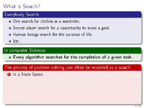
Everybody Search
One search for clothes in a wardrobe.
Soccer player search for a opportunity to score a goal.
Human beings search for the purpose of life.
Etc.
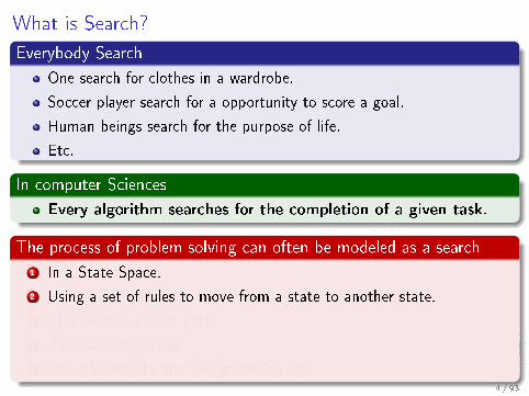
In computer Sciences
Every algorithm searches for the completion of a given task.
The process of problem solving can often be modeled as a search
1 In a State Space.
2 Using a set of rules to move from a state to another state.
3 This creates a state path.
4 To reach some Goal.
5 Often looking by the best possible path.4 / 93

What is Search?
Everybody Search
One search for clothes in a wardrobe.
Soccer player search for a opportunity to score a goal.
Human beings search for the purpose of life.
Etc.
In computer Sciences
Every algorithm searches for the completion of a given task.
The process of problem solving can often be modeled as a search
1 In a State Space.
2 Using a set of rules to move from a state to another state.
3 This creates a state path.
4 To reach some Goal.
5 Often looking by the best possible path.4 / 93

What is Search?
Example
Start Node
Explored NodesFrontier NodesUnexplored Nodes
Figure: Example of Search
5 / 93

State Space Problem
State Space Problem
De�nition
A state space problem P = (S,A, s, T ) consists of a:
1 Set of states S.2 A starting state s3 A set of goal states T ⊆ S.4 A �nite set of actions A = {a1, a2..., an}.
1 Where ai : S → S is a function that transform a stateinto another state.
6 / 93

State Space Problem
State Space Problem
De�nition
A state space problem P = (S,A, s, T ) consists of a:
1 Set of states S.2 A starting state s3 A set of goal states T ⊆ S.4 A �nite set of actions A = {a1, a2..., an}.
1 Where ai : S → S is a function that transform a stateinto another state.
6 / 93
State Space Problem
State Space Problem
De�nition
A state space problem P = (S,A, s, T ) consists of a:
1 Set of states S.2 A starting state s3 A set of goal states T ⊆ S.4 A �nite set of actions A = {a1, a2..., an}.
1 Where ai : S → S is a function that transform a stateinto another state.
6 / 93

State Space Problem
State Space Problem
De�nition
A state space problem P = (S,A, s, T ) consists of a:
1 Set of states S.2 A starting state s3 A set of goal states T ⊆ S.4 A �nite set of actions A = {a1, a2..., an}.
1 Where ai : S → S is a function that transform a stateinto another state.
6 / 93

State Space Problem
State Space Problem
De�nition
A state space problem P = (S,A, s, T ) consists of a:
1 Set of states S.2 A starting state s3 A set of goal states T ⊆ S.4 A �nite set of actions A = {a1, a2..., an}.
1 Where ai : S → S is a function that transform a stateinto another state.
6 / 93

State Space Problem
State Space Problem
De�nition
A state space problem P = (S,A, s, T ) consists of a:
1 Set of states S.2 A starting state s3 A set of goal states T ⊆ S.4 A �nite set of actions A = {a1, a2..., an}.
1 Where ai : S → S is a function that transform a stateinto another state.
6 / 93
Example: RAILROAD SWITCHING
Description
An engine (E) at the siding can push or pull two cars (A and B) on the track.
The railway passes through a tunnel that only the engine, but not the rail cars, can
pass.
GoalTo exchange the location of the two cars and have the engine back on the siding.
7 / 93

Example: RAILROAD SWITCHING
The Structue of the Problem
8 / 93

Outline
1 Motivation
What is Search?
2 State Space Problem
Better Representation
Example
Solution De�nition
Weighted State Space Problem
Evaluation of Search Strategies
3 Uninformed Graph Search Algorithms
Basic Functions
Depth-First Search
Breadth-First Search
Combining DFS and BFS
However, We Have the Results of Solving a Maze
4 Dijkstra's Algorithm: Di�erent ways of doing Stu�
What happened when you have weights?
What to do with negative weights?
Implicit Bellman-Ford
9 / 93

State Space Problem Graph
De�nition
A problem graph G = (V,E, s, T ) for the state space problemP = (S,A, s, T ) is de�ned by:
1 V = S as the set of nodes.
2 s ∈ S as the initial node.
3 T as the set of goal nodes.
4 E ⊆ V × V as the set of edges that connect nodes to nodes with
(u, v) ∈ E if and only if there exists an a ∈ A with a(u) = v.
10 / 93

Outline
1 Motivation
What is Search?
2 State Space Problem
Better Representation
Example
Solution De�nition
Weighted State Space Problem
Evaluation of Search Strategies
3 Uninformed Graph Search Algorithms
Basic Functions
Depth-First Search
Breadth-First Search
Combining DFS and BFS
However, We Have the Results of Solving a Maze
4 Dijkstra's Algorithm: Di�erent ways of doing Stu�
What happened when you have weights?
What to do with negative weights?
Implicit Bellman-Ford
11 / 93

Example
Engine
Car A
Car B
Figure: Possible states are labeled by the locations of the engine (E) and the cars(A and B), either in the form of a string or of a pictogram; EAB is the start state,EBA is the goal state.
12 / 93

Example
Inside of each state you could have
Engine
Car A
Car B
13 / 93

Outline
1 Motivation
What is Search?
2 State Space Problem
Better Representation
Example
Solution De�nition
Weighted State Space Problem
Evaluation of Search Strategies
3 Uninformed Graph Search Algorithms
Basic Functions
Depth-First Search
Breadth-First Search
Combining DFS and BFS
However, We Have the Results of Solving a Maze
4 Dijkstra's Algorithm: Di�erent ways of doing Stu�
What happened when you have weights?
What to do with negative weights?
Implicit Bellman-Ford
14 / 93

Solution
De�nition
A solution π = (a1, a2, ..., ak) is an ordered sequence of actions
ai ∈ A, i ∈ 1, ..., k that transforms the initial state s into one of the goal
states t ∈ T .
Thus
There exists a sequence of states ui ∈ S, i ∈ 0, ..., k, with u0 = s, uk = t,and ui is the outcome of applying ai to ui−1, i ∈ 1, ..., k.
15 / 93

Solution
De�nition
A solution π = (a1, a2, ..., ak) is an ordered sequence of actions
ai ∈ A, i ∈ 1, ..., k that transforms the initial state s into one of the goal
states t ∈ T .
Thus
There exists a sequence of states ui ∈ S, i ∈ 0, ..., k, with u0 = s, uk = t,and ui is the outcome of applying ai to ui−1, i ∈ 1, ..., k.
Problem Space
15 / 93

We want the following
We are interested in!!!
Solution length of a problem i.e. the number of actions in thesequence.
Cost of the solution.
16 / 93

Outline
1 Motivation
What is Search?
2 State Space Problem
Better Representation
Example
Solution De�nition
Weighted State Space Problem
Evaluation of Search Strategies
3 Uninformed Graph Search Algorithms
Basic Functions
Depth-First Search
Breadth-First Search
Combining DFS and BFS
However, We Have the Results of Solving a Maze
4 Dijkstra's Algorithm: Di�erent ways of doing Stu�
What happened when you have weights?
What to do with negative weights?
Implicit Bellman-Ford
17 / 93

It is more
As in Graph Theory
We can add a weight to each edge
We can then
De�ne the Weighted State Space Problem
18 / 93

It is more
As in Graph Theory
We can add a weight to each edge
We can then
De�ne the Weighted State Space Problem
18 / 93

Weighted State Space Problem
De�nition
A weighted state space problem is a tuple P = (S,A, s, T, w), wherew is a cost functionw : A→ R. The cost of a path consisting of
actions a1, ..., an is de�ned as∑n
i=1w (ai).
In a weighted search space, we call a solution optimal, if it hasminimum cost among all feasible solutions.
19 / 93

Then
Observations I
For a weighted state space problem, there is a corresponding weighted
problem graph G = (V,E, s, T, w), where w is extended to E → R in
the straightforward way.
The weight or cost of a path π = (v0, ..., vk) is de�ned as
w (π) =∑k
i=1w (vi−1, vi).
Observations II
δ (s, t) = min {w(π)|π = (v0 = s, ..., vk = t)}The optimal solution cost can be abbreviated as
δ(s, T ) = min {t ∈ T |δ(s, t)}.
20 / 93

Example
The weights
Weighted Problem Space
21 / 93

Notes in Graph Representation
Terms
Node expansion (a.k.a. node exploration):
I Generation of all neighbors of a node u.I This nodes are called successors of u.I u is a parent or predecessor.
In addition...
All nodes u0, ..., un−1 are called antecessors of u.
u is a descendant of each node u0, ..., un−1.
Thus, ancestor and descendant refer to paths of possibly more than
one edge.
22 / 93

Outline
1 Motivation
What is Search?
2 State Space Problem
Better Representation
Example
Solution De�nition
Weighted State Space Problem
Evaluation of Search Strategies
3 Uninformed Graph Search Algorithms
Basic Functions
Depth-First Search
Breadth-First Search
Combining DFS and BFS
However, We Have the Results of Solving a Maze
4 Dijkstra's Algorithm: Di�erent ways of doing Stu�
What happened when you have weights?
What to do with negative weights?
Implicit Bellman-Ford
23 / 93

Evaluation of Search Strategies
Evaluation Parameters
Completeness: Does it always �nd a solution if one exists?
Time complexity: Number of nodes generated.
Space complexity: Maximum number of nodes in memory.
Optimality: Does it always �nd a least-cost solution?
Time and space complexity are measured in terms of...
b: Branching factor of a state is the number of successors it has.
I If Succ(u) abbreviates the successor set of a state u ∈ S then thebranching factor is |Succ(u)|
F That is, cardinality of Succ(u).
δ: Depth of the least-cost solution.
m: Maximum depth of the state space (may be ∞).
24 / 93

Implicit State Space Graph
Reached Nodes
Solving state space problems is sometimes better characterized as a
search in an implicit graph.
The di�erence is that not all edges have to be explicitly stored, but are
generated by a set of rules.
This setting of an implicit generation of the search space is also called
on-the-�y, incremental, or lazy state space generation in some
domains.
25 / 93

A More Complete De�nition
De�nition
In an implicit state space graph, we have
An initial node s ∈ V .A set of goal nodes determined by a predicate
Goal : V → B = {false, true}
A node expansion procedure Expand : V → 2V .
26 / 93

A More Complete De�nition
De�nition
In an implicit state space graph, we have
An initial node s ∈ V .A set of goal nodes determined by a predicate
Goal : V → B = {false, true}
A node expansion procedure Expand : V → 2V .
26 / 93

A More Complete De�nition
De�nition
In an implicit state space graph, we have
An initial node s ∈ V .A set of goal nodes determined by a predicate
Goal : V → B = {false, true}
A node expansion procedure Expand : V → 2V .
26 / 93
A More Complete De�nition
De�nition
In an implicit state space graph, we have
An initial node s ∈ V .A set of goal nodes determined by a predicate
Goal : V → B = {false, true}
A node expansion procedure Expand : V → 2V .
26 / 93

Open and Closed List
Reached Nodes
They are divided into
I Expanded Nodes - Closed ListI Generated Nodes (Still not expanded) - Open List - Search Frontier
Search Tree
The set of all explicitly generated paths rooted at the start node(leaves = Open Nodes) constitutes the search tree of theunderlying problem graph.
27 / 93

Example
Problem Graph
Figure: Problem Graph
28 / 93
Outline
1 Motivation
What is Search?
2 State Space Problem
Better Representation
Example
Solution De�nition
Weighted State Space Problem
Evaluation of Search Strategies
3 Uninformed Graph Search Algorithms
Basic Functions
Depth-First Search
Breadth-First Search
Combining DFS and BFS
However, We Have the Results of Solving a Maze
4 Dijkstra's Algorithm: Di�erent ways of doing Stu�
What happened when you have weights?
What to do with negative weights?
Implicit Bellman-Ford
29 / 93

Skeleton of a Search Algorithm
Basic Algorithm
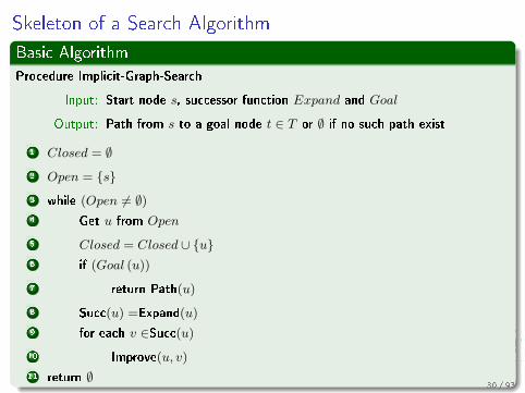
Procedure Implicit-Graph-Search
Input: Start node s, successor function Expand and Goal
Output: Path from s to a goal node t ∈ T or ∅ if no such path exist
1 Closed = ∅2 Open = {s}3 while (Open 6= ∅)4 Get u from Open
5 Closed = Closed ∪ {u}6 if (Goal (u))
7 return Path(u)
8 Succ(u) =Expand(u)
9 for each v ∈Succ(u)10 Improve(u, v)
11 return ∅30 / 93

Skeleton of a Search Algorithm
Basic Algorithm
Procedure Implicit-Graph-Search
Input: Start node s, successor function Expand and Goal
Output: Path from s to a goal node t ∈ T or ∅ if no such path exist
1 Closed = ∅2 Open = {s}3 while (Open 6= ∅)4 Get u from Open
5 Closed = Closed ∪ {u}6 if (Goal (u))
7 return Path(u)
8 Succ(u) =Expand(u)
9 for each v ∈Succ(u)10 Improve(u, v)
11 return ∅30 / 93

Improve Algorithm
Basic Algorithm
Improve
Input: Nodes u and v, v successor of u
Output: Update parent v, Open and Closed
1 if (v /∈ Closed ∪Open)2 Insert v into Open
3 parent (v) = u
31 / 93

Returning the Path
Basic Algorithm
Procedure Path
Input: Node u, start node s and parents set by the algorithm
Output: Path from s to u
1 Path = Path ∪ {u}2 while (parent (u) 6= s)
3 u = parent (u)
4 Path = Path ∪ {u}
32 / 93

Algorithms to be Explored
Algorithm
1 Depth-First Search
2 Breadth-First Search
3 Dijkstra's Algorithm
4 Relaxed Node Selection
5 Bellman-Ford
6 Dynamic Programming
33 / 93

Outline
1 Motivation
What is Search?
2 State Space Problem
Better Representation
Example
Solution De�nition
Weighted State Space Problem
Evaluation of Search Strategies
3 Uninformed Graph Search Algorithms
Basic Functions
Depth-First Search
Breadth-First Search
Combining DFS and BFS
However, We Have the Results of Solving a Maze
4 Dijkstra's Algorithm: Di�erent ways of doing Stu�
What happened when you have weights?
What to do with negative weights?
Implicit Bellman-Ford
34 / 93
Depth First Search
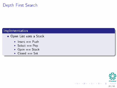
Implementation
Open List uses a Stack
I Insert == PushI Select == PopI Open == StackI Closed == Set
35 / 93

Example of the Implicit Graph
Something Notable
S
UNEXPLORED STATES
CLOSED
OPEN
36 / 93

BTW
Did you notice the following? Given X a search space
Open ∩ Closed == ∅X−(Open ∪ Closed) ∩ Open == ∅X−(Open ∪ Closed) ∩ Closed == ∅
Disjoint Set Representation
Yes!!! We can do it!!!
For the Closed set!!!
37 / 93

BTW
Did you notice the following? Given X a search space
Open ∩ Closed == ∅X−(Open ∪ Closed) ∩ Open == ∅X−(Open ∪ Closed) ∩ Closed == ∅
Disjoint Set Representation
Yes!!! We can do it!!!
For the Closed set!!!
37 / 93

How DFS measures?
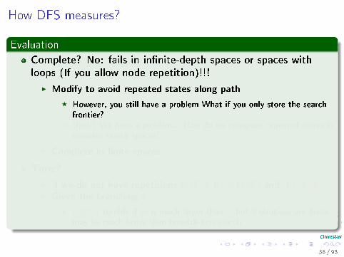
Evaluation
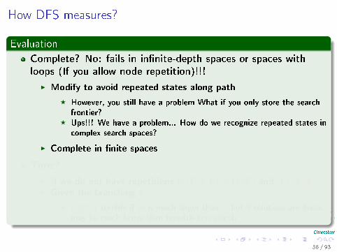
Complete? No: fails in in�nite-depth spaces or spaces withloops (If you allow node repetition)!!!
I Modify to avoid repeated states along path
F However, you still have a problem What if you only store the searchfrontier?
F Ups!!! We have a problem... How do we recognize repeated states incomplex search spaces?
I Complete in �nite spaces
Time?
I If we do not have repetitions O (V + E) = O (E) and |V | � |E|I Given the branching b:
F O(bm): terrible if m is much larger than δ, but if solutions are dense,may be much faster than breadth-�rst search
38 / 93

How DFS measures?
Evaluation
Complete? No: fails in in�nite-depth spaces or spaces withloops (If you allow node repetition)!!!
I Modify to avoid repeated states along path
F However, you still have a problem What if you only store the searchfrontier?
F Ups!!! We have a problem... How do we recognize repeated states incomplex search spaces?
I Complete in �nite spaces
Time?
I If we do not have repetitions O (V + E) = O (E) and |V | � |E|I Given the branching b:
F O(bm): terrible if m is much larger than δ, but if solutions are dense,may be much faster than breadth-�rst search
38 / 93
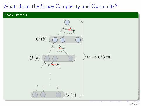
What about the Space Complexity and Optimality?
Look at this
39 / 93

Optimal? No, look at the following example...
Example
No so niceDFS
1
1 2 3
2
3
4
5
4 5
Figure: Goal at (5,1) from node (3,3)
40 / 93

The Pseudo-Code - Solving the Problem of Repeated Nodes
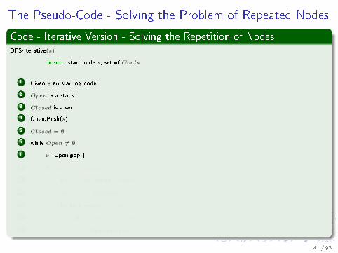
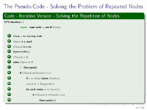
Code - Iterative Version - Solving the Repetition of NodesDFS-Iterative(s)
Input: start node s, set of Goals
1 Given s an starting node
2 Open is a stack
3 Closed is a set
4 Open.Push(s)
5 Closed = ∅
6 while Open 6= ∅
7 v=Open.pop()
8 if Closed 6=Closed ∪ (v)
9 if v ∈ Goal return Path(v)
10 succ(v) = Expand(v)
11 for each vertex u ∈ succ(v)
12 if Closed 6= Closed ∪ (u)
13 Open.push(u)
41 / 93

The Pseudo-Code - Solving the Problem of Repeated Nodes
Code - Iterative Version - Solving the Repetition of NodesDFS-Iterative(s)
Input: start node s, set of Goals
1 Given s an starting node
2 Open is a stack
3 Closed is a set
4 Open.Push(s)
5 Closed = ∅
6 while Open 6= ∅
7 v=Open.pop()
8 if Closed 6=Closed ∪ (v)
9 if v ∈ Goal return Path(v)
10 succ(v) = Expand(v)
11 for each vertex u ∈ succ(v)
12 if Closed 6= Closed ∪ (u)
13 Open.push(u)
41 / 93

Why?
Using our Disjoint Set Representation
We get the ability to be able to compare two sets through the
representatives!!!
Not only that
Using that, we solve the problem of node repetition
Little Problem
If we are only storing the frontier our disjoint set representation is not
enough!!!
More research is needed!!!
42 / 93

Example
Example
43 / 93

Example
The numbers in brackets denote the order of node generation.
44 / 93

Outline
1 Motivation
What is Search?
2 State Space Problem
Better Representation
Example
Solution De�nition
Weighted State Space Problem
Evaluation of Search Strategies
3 Uninformed Graph Search Algorithms
Basic Functions
Depth-First Search
Breadth-First Search
Combining DFS and BFS
However, We Have the Results of Solving a Maze
4 Dijkstra's Algorithm: Di�erent ways of doing Stu�
What happened when you have weights?
What to do with negative weights?
Implicit Bellman-Ford
45 / 93

Bradth-First Search
Implementation
Open List uses a Queue
I Insert == EnqueueI Select == DequeueI Open == QueueI Closed == Set
46 / 93

Breast-First Search Pseudo-Code
BFS-Implicit(s)
Input: start node s, set of Goals
1 Open is a queue
2 Closed is a set
3 Open.enqueue(s)
4 Closed = ∅5 while Open 6= ∅6 v = Open.dequeue()
7 if Closed 6=Closed ∪ (v)
8 if v ∈ Goal return Path(v)9 succ(v) = Expand(v)
10 for each vertex u ∈ succ(v)11 if Closed 6= Closed ∪ (u)
12 Open.enqueue(u)
47 / 93

How BFS measures?
Evaluation
Complete? Yes if b is �nite
Time? 1 + b+ b2 + b3 + . . .+ bδ = O(bδ)
Space? O(bδ)This is a big problem
Optimal? Yes, If cost is equal for each step.
48 / 93

How BFS measures?
Evaluation
Complete? Yes if b is �nite
Time? 1 + b+ b2 + b3 + . . .+ bδ = O(bδ)
Space? O(bδ)This is a big problem
Optimal? Yes, If cost is equal for each step.
48 / 93

How BFS measures?
Evaluation
Complete? Yes if b is �nite
Time? 1 + b+ b2 + b3 + . . .+ bδ = O(bδ)
Space? O(bδ)This is a big problem
Optimal? Yes, If cost is equal for each step.
48 / 93

How BFS measures?
Evaluation
Complete? Yes if b is �nite
Time? 1 + b+ b2 + b3 + . . .+ bδ = O(bδ)
Space? O(bδ)This is a big problem
Optimal? Yes, If cost is equal for each step.
48 / 93

Example
Example
49 / 93

Example
The numbers in brackets denote the order of node generation.
50 / 93
Outline
1 Motivation
What is Search?
2 State Space Problem
Better Representation
Example
Solution De�nition
Weighted State Space Problem
Evaluation of Search Strategies
3 Uninformed Graph Search Algorithms
Basic Functions
Depth-First Search
Breadth-First Search
Combining DFS and BFS
However, We Have the Results of Solving a Maze
4 Dijkstra's Algorithm: Di�erent ways of doing Stu�
What happened when you have weights?
What to do with negative weights?
Implicit Bellman-Ford
51 / 93

Can we combine the bene�ts of both algorithms?
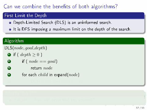
First Limit the Depth
Depth-Limited Search (DLS) is an uninformed search.
It is DFS imposing a maximum limit on the depth of the search.
Algorithm
DLS(node, goal,depth)
1 if ( depth ≥ 0 )
2 if ( node == goal)
3 return node
4 for each child in expand(node)
5 DLS(child, goal, depth− 1)
IMPORTANT!!!
If depth < δ we will never �nd the answer!!!
52 / 93

Can we combine the bene�ts of both algorithms?
First Limit the Depth
Depth-Limited Search (DLS) is an uninformed search.
It is DFS imposing a maximum limit on the depth of the search.
Algorithm
DLS(node, goal,depth)
1 if ( depth ≥ 0 )
2 if ( node == goal)
3 return node
4 for each child in expand(node)
5 DLS(child, goal, depth− 1)
IMPORTANT!!!
If depth < δ we will never �nd the answer!!!
52 / 93

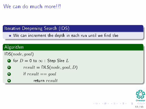
We can do much more!!!
Iterative Deepening Search (IDS)
We can increment the depth in each run until we �nd the
Algorithm
IDS(node, goal)
1 for D = 0 to ∞ : Step Size L
2 result = DLS(node, goal,D)
3 if result == goal
4 return result
53 / 93
We can do much more!!!
Iterative Deepening Search (IDS)
We can increment the depth in each run until we �nd the
Algorithm
IDS(node, goal)
1 for D = 0 to ∞ : Step Size L
2 result = DLS(node, goal,D)
3 if result == goal
4 return result
53 / 93

Example
Example: D == 1
54 / 93

Example
Example: D == 1
55 / 93

Example
Example: D == 1
56 / 93
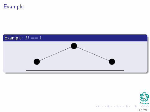
Example
Example: D == 1
57 / 93

Example
Example: D == 2
58 / 93

Example
Example: D == 2
59 / 93

Example
Example: D == 2
60 / 93

Example
Example: depth == 2
61 / 93

Example
Example: depth == 2
62 / 93

Example
Example: depth == 2
63 / 93

Properties of IDS
Properties
Complete? Yes
Time? δb1 + (δ − 1)b2 + . . .+ bδ = O(bδ)
Space? O (δb)
Optimal? Yes, if step cost = 1
64 / 93

Properties of IDS
Properties
Complete? Yes
Time? δb1 + (δ − 1)b2 + . . .+ bδ = O(bδ)
Space? O (δb)
Optimal? Yes, if step cost = 1
64 / 93

Properties of IDS
Properties
Complete? Yes
Time? δb1 + (δ − 1)b2 + . . .+ bδ = O(bδ)
Space? O (δb)
Optimal? Yes, if step cost = 1
64 / 93

Properties of IDS
Properties
Complete? Yes
Time? δb1 + (δ − 1)b2 + . . .+ bδ = O(bδ)
Space? O (δb)
Optimal? Yes, if step cost = 1
64 / 93

Iterative Deepening Search Works
Setup - Thanks to Felipe 2015 Class
Dk the search depth in the algorithm at step k in the wrap part of the
algorithm
I Which can have certain step size!!!
65 / 93

Iterative Deepening Search Works
Theorem (IDS works)
Let dminmin the minimum depth of all goal states in the search tree rooted
at s. Suppose that
Dk−1 < dmin ≤ Dk
where D0 = 0. Then IDS will �nd a goal whose depth is as much Dk.
66 / 93
Iterative Deepening Search Works
Theorem (IDS works)
Let dminmin the minimum depth of all goal states in the search tree rooted
at s. Suppose that
Dk−1 < dmin ≤ Dk
where D0 = 0. Then IDS will �nd a goal whose depth is as much Dk.
66 / 93

Proof
Since b > 0 and �nite
We know that the algorithm Depth-Limited Search has no vertices below
depth D making the tree �nite
In addition
A dept-�rst search will �nd the solution in such a tree if any exist.
By de�nition of dmin
The tree generated by Depth-Limited Search must have a goal if and only
if D ≥ dmin.
67 / 93

Proof
Thus
No goal can be �nd until D = Dk at which time a goal will be found.
Because
The Goal is in the tree, its depth is at most Dk.
68 / 93

Proof
Thus
No goal can be �nd until D = Dk at which time a goal will be found.
Because
The Goal is in the tree, its depth is at most Dk.
68 / 93

Iterative Deepening Search Problems
Theorem (Upper Bound of calls to IDS)
Suppose that Dk = k and b > 1 (Branching greater than one) for all
non-goal vertices s. Let be I the number of calls to Depth Limited Search
until a solution is found. Let L be the number of vertices placed in the
queue by the BFS. Then, I < 3 (L+ 1).
Note
The theorem points that at least that IDS will be called at most 3
times the number of vertices placed in the queue by BFS.
69 / 93

Proof
Claim
Suppose b > 1 for any nongoal vertex. Let κ be the least depth of any
goal.
Let dk be the number of vertices in the search tree at depth k.
Let mk be the number of vertices at depth less than k.
Thus, for k ≤ κ
We have that
mk < dk
mk−1 <12mk
Proof
I leave this to you
70 / 93

Proof
Claim
Suppose b > 1 for any nongoal vertex. Let κ be the least depth of any
goal.
Let dk be the number of vertices in the search tree at depth k.
Let mk be the number of vertices at depth less than k.
Thus, for k ≤ κ
We have that
mk < dk
mk−1 <12mk
Proof
I leave this to you
70 / 93

Proof
Claim
Suppose b > 1 for any nongoal vertex. Let κ be the least depth of any
goal.
Let dk be the number of vertices in the search tree at depth k.
Let mk be the number of vertices at depth less than k.
Thus, for k ≤ κ
We have that
mk < dk
mk−1 <12mk
Proof
I leave this to you
70 / 93

Proof
Claim
Suppose b > 1 for any nongoal vertex. Let κ be the least depth of any
goal.
Let dk be the number of vertices in the search tree at depth k.
Let mk be the number of vertices at depth less than k.
Thus, for k ≤ κ
We have that
mk < dk
mk−1 <12mk
Proof
I leave this to you
70 / 93
Proof
Claim
Suppose b > 1 for any nongoal vertex. Let κ be the least depth of any
goal.
Let dk be the number of vertices in the search tree at depth k.
Let mk be the number of vertices at depth less than k.
Thus, for k ≤ κ
We have that
mk < dk
mk−1 <12mk
Proof
I leave this to you
70 / 93

Proof
Claim
Suppose b > 1 for any nongoal vertex. Let κ be the least depth of any
goal.
Let dk be the number of vertices in the search tree at depth k.
Let mk be the number of vertices at depth less than k.
Thus, for k ≤ κ
We have that
mk < dk
mk−1 <12mk
Proof
I leave this to you
70 / 93

Proof
Claim
Suppose b > 1 for any nongoal vertex. Let κ be the least depth of any
goal.
Let dk be the number of vertices in the search tree at depth k.
Let mk be the number of vertices at depth less than k.
Thus, for k ≤ κ
We have that
mk < dk
mk−1 <12mk
Proof
I leave this to you
70 / 93

Proof
Thus, we have
mk <1
2mk+1 <
(1
2
)2
mk+1 < ... <
(1
2
)κ−kmκ (1)
Suppose
The �rst goal encountered by the BFS is the nth vertex at depth κ .
Let
L = mκ + n− 1 (2)
because the goal is not placed on the queue of the BFS.
71 / 93

Proof
Thus, we have
mk <1
2mk+1 <
(1
2
)2
mk+1 < ... <
(1
2
)κ−kmκ (1)
Suppose
The �rst goal encountered by the BFS is the nth vertex at depth κ .
Let
L = mκ + n− 1 (2)
because the goal is not placed on the queue of the BFS.
71 / 93

Proof
Thus, we have
mk <1
2mk+1 <
(1
2
)2
mk+1 < ... <
(1
2
)κ−kmκ (1)
Suppose
The �rst goal encountered by the BFS is the nth vertex at depth κ .
Let
L = mκ + n− 1 (2)
because the goal is not placed on the queue of the BFS.
71 / 93

Proof
The total number of call of DLS
For Dk = k < κ is
mk + dk (3)
72 / 93
Proof
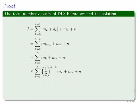
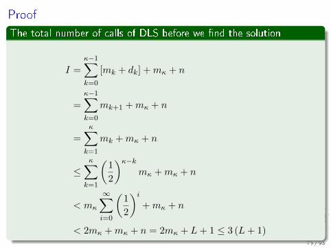
The total number of calls of DLS before we �nd the solution
I =
κ−1∑k=0
[mk + dk] +mκ + n
=
κ−1∑k=0
mk+1 +mκ + n
=
κ∑k=1
mk +mκ + n
≤κ∑k=1
(1
2
)κ−kmκ +mκ + n
< mκ
∞∑i=0
(1
2
)i+mκ + n
< 2mκ +mκ + n = 2mκ + L+ 1 ≤ 3 (L+ 1)73 / 93

Proof
The total number of calls of DLS before we �nd the solution
I =
κ−1∑k=0
[mk + dk] +mκ + n
=
κ−1∑k=0
mk+1 +mκ + n
=
κ∑k=1
mk +mκ + n
≤κ∑k=1
(1
2
)κ−kmκ +mκ + n
< mκ
∞∑i=0
(1
2
)i+mκ + n
< 2mκ +mκ + n = 2mκ + L+ 1 ≤ 3 (L+ 1)73 / 93

Proof
The total number of calls of DLS before we �nd the solution
I =
κ−1∑k=0
[mk + dk] +mκ + n
=
κ−1∑k=0
mk+1 +mκ + n
=
κ∑k=1
mk +mκ + n
≤κ∑k=1
(1
2
)κ−kmκ +mκ + n
< mκ
∞∑i=0
(1
2
)i+mκ + n
< 2mκ +mκ + n = 2mκ + L+ 1 ≤ 3 (L+ 1)73 / 93
Proof
The total number of calls of DLS before we �nd the solution
I =
κ−1∑k=0
[mk + dk] +mκ + n
=
κ−1∑k=0
mk+1 +mκ + n
=
κ∑k=1
mk +mκ + n
≤κ∑k=1
(1
2
)κ−kmκ +mκ + n
< mκ
∞∑i=0
(1
2
)i+mκ + n
< 2mκ +mκ + n = 2mκ + L+ 1 ≤ 3 (L+ 1)73 / 93

Proof
The total number of calls of DLS before we �nd the solution
I =
κ−1∑k=0
[mk + dk] +mκ + n
=
κ−1∑k=0
mk+1 +mκ + n
=
κ∑k=1
mk +mκ + n
≤κ∑k=1
(1
2
)κ−kmκ +mκ + n
< mκ
∞∑i=0
(1
2
)i+mκ + n
< 2mκ +mκ + n = 2mκ + L+ 1 ≤ 3 (L+ 1)73 / 93
Proof
The total number of calls of DLS before we �nd the solution
I =
κ−1∑k=0
[mk + dk] +mκ + n
=
κ−1∑k=0
mk+1 +mκ + n
=
κ∑k=1
mk +mκ + n
≤κ∑k=1
(1
2
)κ−kmκ +mκ + n
< mκ
∞∑i=0
(1
2
)i+mκ + n
< 2mκ +mκ + n = 2mκ + L+ 1 ≤ 3 (L+ 1)73 / 93

Outline
1 Motivation
What is Search?
2 State Space Problem
Better Representation
Example
Solution De�nition
Weighted State Space Problem
Evaluation of Search Strategies
3 Uninformed Graph Search Algorithms
Basic Functions
Depth-First Search
Breadth-First Search
Combining DFS and BFS
However, We Have the Results of Solving a Maze
4 Dijkstra's Algorithm: Di�erent ways of doing Stu�
What happened when you have weights?
What to do with negative weights?
Implicit Bellman-Ford
74 / 93

In the Class of 2014
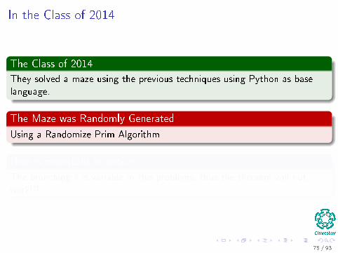
The Class of 2014
They solved a maze using the previous techniques using Python as base
language.
The Maze was Randomly Generated
Using a Randomize Prim Algorithm
Here is important to notice
The branching b is variable in this problems, thus the theorem will not
work!!!
75 / 93
In the Class of 2014
The Class of 2014
They solved a maze using the previous techniques using Python as base
language.
The Maze was Randomly Generated
Using a Randomize Prim Algorithm
Here is important to notice
The branching b is variable in this problems, thus the theorem will not
work!!!
75 / 93

In the Class of 2014
The Class of 2014
They solved a maze using the previous techniques using Python as base
language.
The Maze was Randomly Generated
Using a Randomize Prim Algorithm
Here is important to notice
The branching b is variable in this problems, thus the theorem will not
work!!!
75 / 93

Table Maze Example
Thanks to Lea and Orlando Class 2014 Cinvestav
Size of Maze 40×20
Start (36, 2)
Goal (33, 7)
Algorithm Expanded Nodes Generated Nodes Path Size #Iterations
DFS 482 502 35 NA
BFS 41 47 9 NA
IDS 1090 3197 9 9
IDA* 11 20 9 2
76 / 93

Outline
1 Motivation
What is Search?
2 State Space Problem
Better Representation
Example
Solution De�nition
Weighted State Space Problem
Evaluation of Search Strategies
3 Uninformed Graph Search Algorithms
Basic Functions
Depth-First Search
Breadth-First Search
Combining DFS and BFS
However, We Have the Results of Solving a Maze
4 Dijkstra's Algorithm: Di�erent ways of doing Stu�
What happened when you have weights?
What to do with negative weights?
Implicit Bellman-Ford
77 / 93
Weights in the Implicit Graph
Wights in a Graph
Until now, we have been looking to implicit graphs without weights.
What to do if we have a function w : E → R such that there is a
variability in expanding each path!!!
Algorithms to attack the problem
Dijkstra's Algorithm
Bellman-Ford Algorithm
78 / 93

Clearly somethings need to be taken into account!!!
Implementation
Open List uses a Queue
I MIN Queue Q == GRAYI Out of the Queue Q == BLACKI Update == Relax
79 / 93

Dijkstra's algorithm
DIJKSTRA(s, w)
1 Open is a MIN queue
2 Closed is a set
3 Open.enqueue(s)
4 Closed = ∅5 while Open 6= ∅6 u =Extract-Min(Q)
7 if Closed 6=Closed ∪ (u)
8 succ(u) = Expand(u)
9 for each vertex v ∈ succ(u)10 if Closed 6= Closed ∪ (v)
11 Relax(u, v, w)
12 Closed = Closed ∪ {u}
80 / 93

Relax Procedure
Basic Algorithm
Procedure Relax(u, v, w)
Input: Nodes u, v and v successor of u
SideE�ects: Update parent of v, distance to origin f (v), Open and Closed
1 if (v ∈ Open)⇒Node generated but not expanded
2 if (f (u) + w (u, v) < f (v))
3 parent (v) = u
4 f (v) = f (u) + w (u, v)
5 else6 if (v /∈ Closed)⇒Not yet expanded
7 parent (v) = u
8 f (v) = f (u) + w (u, v)
9 Insert v into Open with f (v)
81 / 93

Complexity
Worst Case Performance - Time Complexity
O (E + V log V ) (4)
Space Complexity
O(V 2)
(5)
82 / 93

Complexity
Worst Case Performance - Time Complexity
O (E + V log V ) (4)
Space Complexity
O(V 2)
(5)
82 / 93

Correctness Dijkstra's Algorithm
Theorem (Optimality of Dijkstra's)
In weighted graphs with nonnegative weight function the algorithm of
Dijkstra's algorithm is optimal.
Proof
With nonnegative edge weights, for each pair (u, v) with Succ (u)f (u) ≤ f (v).Therefore, the values f for selected nodes are monotonically increasing.
This proves that at the �rst selected node t ∈ T , we havef (t) = δ (s, t) = δ (s, T )
83 / 93

Correctness Dijkstra's Algorithm
Theorem (Correctness of Dijkstra's)
If the weight function w of a problem graph G = (V,E,w) is strictlypositive and if the weight of every in�nite path is in�nite, then Dijkstra's
algorithm terminates with an optimal solution.
Proof
The premises induce that if the cost of a path is �nite, the path itself
is �nite.
Observation: There is no path cost ≥ δ (s, T ) can be a pre�x of an
optimal solution path.
Therefore Dijkstra's algorithm examines the problem graph only on a
�nite subset of all in�nite paths.
A goal node t ∈ T with δ (s, t) = δ (s, T ) will eventually, so Dijkstra's
terminates.
By theorem 2.1 the solution will be optimal.
84 / 93

Example
Example
85 / 93
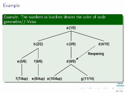
Example
Example: The numbers in brackets denote the order of nodegeneration/f -Value
86 / 93

Outline
1 Motivation
What is Search?
2 State Space Problem
Better Representation
Example
Solution De�nition
Weighted State Space Problem
Evaluation of Search Strategies
3 Uninformed Graph Search Algorithms
Basic Functions
Depth-First Search
Breadth-First Search
Combining DFS and BFS
However, We Have the Results of Solving a Maze
4 Dijkstra's Algorithm: Di�erent ways of doing Stu�
What happened when you have weights?
What to do with negative weights?
Implicit Bellman-Ford
87 / 93
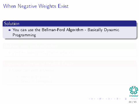
When Negative Weights Exist
Solution
You can use the Bellman-Ford Algorithm - Basically Dynamic
Programming
Bellman uses node relaxation
f(v)← min {f(v), f(u) + w(u, v)}
Implementation on an Implicit Graph
Open List uses a Queue
I Insert = EnqueueI Select = Denqueue
88 / 93

When Negative Weights Exist
Solution
You can use the Bellman-Ford Algorithm - Basically Dynamic
Programming
Bellman uses node relaxation
f(v)← min {f(v), f(u) + w(u, v)}
Implementation on an Implicit Graph
Open List uses a Queue
I Insert = EnqueueI Select = Denqueue
88 / 93

When Negative Weights Exist
Solution
You can use the Bellman-Ford Algorithm - Basically Dynamic
Programming
Bellman uses node relaxation
f(v)← min {f(v), f(u) + w(u, v)}
Implementation on an Implicit Graph
Open List uses a Queue
I Insert = EnqueueI Select = Denqueue
88 / 93

Outline
1 Motivation
What is Search?
2 State Space Problem
Better Representation
Example
Solution De�nition
Weighted State Space Problem
Evaluation of Search Strategies
3 Uninformed Graph Search Algorithms
Basic Functions
Depth-First Search
Breadth-First Search
Combining DFS and BFS
However, We Have the Results of Solving a Maze
4 Dijkstra's Algorithm: Di�erent ways of doing Stu�
What happened when you have weights?
What to do with negative weights?
Implicit Bellman-Ford
89 / 93

Implicit Bellman-Ford
Procedure Implicit Bellman-Ford
Input: Start node s, function w, function Expand and function
Goal
Output: Cheapest path from s to t ∈ T stored in f (s)
1 Open← {s}2 f (s)← h (s)
3 while (Open 6= ∅)4 u = Open.dequeue()
5 Closed = Closed ∪ {u}6 Succ (u)← Expand (u)
7 for each v ∈ Succ (u)8 improve (u, v)
90 / 93
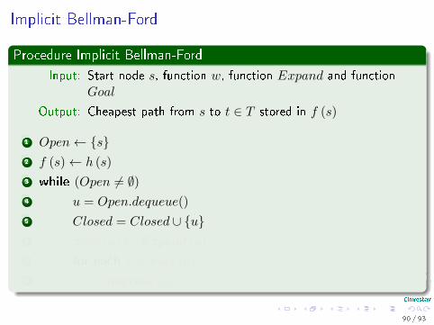
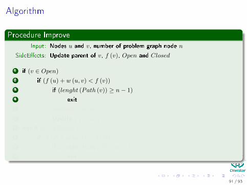
Algorithm
Procedure Improve
Input: Nodes u and v, number of problem graph node n
SideE�ects: Update parent of v, f (v), Open and Closed
1 if (v ∈ Open)2 if (f (u) + w (u, v) < f (v))
3 if (lenght (Path (v)) ≥ n− 1)
4 exit
5 parent (v)← u
6 Update f (v)← f (u) + w (u, v)
7 else if (v ∈ Closed)8 if (f (u) + w (u, v) < f (v))
9 if (lenght (Path (v)) ≥ n− 1)
10 exit
91 / 93
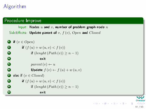
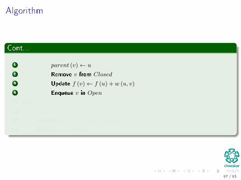
Algorithm
Cont...
1 parent (v)← u
2 Remove v from Closed
3 Update f (v)← f (u) + w (u, v)
4 Enqueue v in Open
5 else
6 parent (v)← u
7 Initialize f (v)← f (u) + w (u, v)
8 Enqueue v in Open
92 / 93
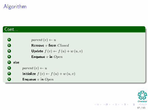
Algorithm
Cont...
1 parent (v)← u
2 Remove v from Closed
3 Update f (v)← f (u) + w (u, v)
4 Enqueue v in Open
5 else
6 parent (v)← u
7 Initialize f (v)← f (u) + w (u, v)
8 Enqueue v in Open
92 / 93
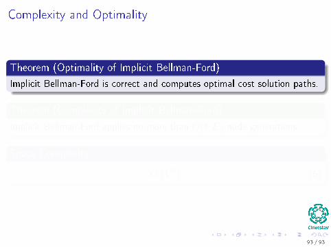
Complexity and Optimality
Theorem (Optimality of Implicit Bellman-Ford)
Implicit Bellman-Ford is correct and computes optimal cost solution paths.
Theorem (Complexity of Implicit Bellman-Ford)
Implicit Bellman-Ford applies no more than O(V E) node generations.
Space Complexity
O(V 2)
(6)
93 / 93
Complexity and Optimality
Theorem (Optimality of Implicit Bellman-Ford)
Implicit Bellman-Ford is correct and computes optimal cost solution paths.
Theorem (Complexity of Implicit Bellman-Ford)
Implicit Bellman-Ford applies no more than O(V E) node generations.
Space Complexity
O(V 2)
(6)
93 / 93

Complexity and Optimality
Theorem (Optimality of Implicit Bellman-Ford)
Implicit Bellman-Ford is correct and computes optimal cost solution paths.
Theorem (Complexity of Implicit Bellman-Ford)
Implicit Bellman-Ford applies no more than O(V E) node generations.
Space Complexity
O(V 2)
(6)
93 / 93