artificial intelligence-aided receiver for a cp-free ofdm
TRANSCRIPT

arX
iv:1
903.
0476
6v2
[cs
.IT
] 4
May
201
91
Artificial Intelligence-aided Receiver for A
CP-Free OFDM System: Design, Simulation,
and Experimental Test
Jing Zhang∗, Chao-Kai Wen†, Shi Jin∗, Geoffrey Ye Li‡
∗ National Mobile Communications Research Laboratory, Southeast University
Nanjing 210096, P. R. China, Email: {jingzhang, jinshi}@seu.edu.cn
† Institute of Communications Engineering, Taiwan Sun Yat-sen University
Kaohsiung 80424, Taiwan, Email: [email protected]
‡ School of Electrical and Computer Engineering, Georgia Institute of Technology
Atlanta, GA 30332, USA, Email: [email protected].
Abstract
Orthogonal frequency division multiplexing (OFDM), usually with sufficient cyclic prefix (CP), has
been widely applied in various communication systems. The CP in OFDM consumes additional resource
and reduces spectrum and energy efficiency. However, channel estimation and signal detection are very
challenging for CP-free OFDM systems. In this paper, we propose a novel artificial intelligence (AI)-
aided receiver (AI receiver) for a CP-free OFDM system. The AI receiver includes a channel estimation
neural network (CE-NET) and a signal detection neural network based on orthogonal approximate
message passing (OAMP), called OAMP-NET. The CE-NET is initialized by the least-square channel
estimation algorithm and refined by a linear minimum mean-squared error neural network. The OAMP-
NET is established by unfolding the iterative OAMP algorithm and adding several trainable parameters
to improve the detection performance. We first investigate their performance under different channel
models through extensive simulation and then establish a real transmission system using a 5G rapid
prototyping system for an over-the-air (OTA) test. Based on our study, the AI receiver can estimate
This work was supported in part by the National Science Foundation (NSFC) for Distinguished Young Scholars of China
with Grant 61625106, and in part by the NSFC under Grant 61531011. The work of C.-K. Wen was supported by the Ministry
of Science and Technology of Taiwan under Grants MOST 107-2221-E-110-026 and the ITRI in Hsinchu, Taiwan.

2
time-varying channels with a single training phase. It also has great robustness to various imperfections
and has better performance than those competitive algorithms, especially for high-order modulation.
The OTA test further verifies its feasibility to real environments and indicates its potential for future
communications systems.
Index Terms
OFDM, CP-free, AI, message passing, OTA
I. INTRODUCTION
Orthogonal frequency division multiplexing (OFDM) can effectively deal with delay spread
of wireless channels and therefore it has been used in almost all wireless systems [1]. To
completely mitigate inter-OFDM-block interference (IBI), enough cyclic prefix (CP) must be
inserted between adjacent OFDM blocks, which reduces spectral efficiency of OFDM systems,
especially when the delay spread is large or the OFDM block duration is short as in many
Internet of things (IoT) applications [2]. Without sufficient CP, demodulated OFDM signals will
suffer from inter-carrier interference (ICI) in addition to IBI.
To deal with the IBI and ICI induced by insufficient CP, several techniques [3]–[9] have been
proposed for OFDM. An iterative strategy, called residual inter-symbol interference cancellation
(RISIC), has been developed in [3], [4], [6] to mitigate the IBI, which can achieve an acceptable
performance if the channel delay spread is moderate. A CP-free OFDM scheme in [5], called
symbol cyclic-shift equalization algorithm, includes decision-feedback equalization (DFE) and
CP restoration units. To deal with the sensitivity of DFE to the feedback delay, stored feedback
equalization is used in [10] to eliminate the ISI, which however causes low detection accuracy.
The impact of removing the CP in OFDM in massive multiple-input multiple-output (MIMO)
systems has been investigated in [7]–[9]. In addition to signal detection, channel estimation is
another challenging issue because the received pilot signals are influenced by CP removal. We
will use artificial intelligence (AI) to address both channel estimation and signal detection in a
CP-free OFDM system.
Intelligent communication is considered one of the mainstream directions in the development
of wireless communications after 5G. By introducing AI into wireless communications, system
performance can be potentially improved. Deep learning for wireless systems is in the preliminary
exploration stage, many achievements have transpired in wireless physical layers [11], including

3
channel estimation [12], signal detection [13], feedback and reconstruction of channel state
information (CSI) [14], [15], channel decoding [16], and end-to-end wireless-communication
systems [17] [18].
Deep learning (DL) has been recently introduced to OFDM receivers owing to its strong
ability to perform channel estimation and signal detection, as well as to address the transceiver’s
imperfection [19], [20]. DL approaches can be classified into two categories: data-driven and
model-driven [11]. Data-driven DL techniques generally utilize the standard neural network
structure as a black box and are trained by a huge data set. In contrast to data-driven DL, model-
driven DL methods construct the network topology according to known physical mechanisms
and expert knowledge, and therefore require less training data and shorter training time [21].
Both types of DL have been used in OFDM receivers [22]–[27]. A novel data-driven DL
architecture has been developed in [22] for an OFDM receiver with one-bit complex quantization.
In [23], Cascade-Net has been proposed for signal detection in an OFDM system with sufficient
CP, where deep neural network is cascaded with a zero-forcing preprocessor to prevent the
network stucking in a saddle point or a local minimum point. The Cascade-Net, which can be
regarded as model-driven DL, outperforms zero-forcing method and provides robustness against
ill conditioned channels. An intelligent OFDM receiver has been proposed in [24] based on a
deep complex convolutional network. Its performance is comparable to the traditional receiver for
a CP-free OFDM system based on expert knowledge in additive white Gaussian noise (AWGN)
channels. However, its performance declines precipitously for multi-path fading channel. In [25],
a fully-connected deep neural network (FC-DNN) has been used for channel estimation and
signal detection, which also works well even for a CP-free OFDM system with quadrature
phase shift keying (QPSK) modulation. A model-driven DL method, named ComNet, has been
developed in [26] to improve the performance of the OFDM receiver, especially with high-
order modulation. Since a recurrent neural network is applied in ComNet, it can improve signal
detection performance but has high complexity at the same time. The performance of FC-DNN
and ComNet has been compared in [27]. The trainable iterative soft thresholding algorithm
(TISTA) in [28], which is also a model-driven method, unfolds the orthogonal approximate
message passing (OAMP) algorithm and trains some variables by DL to solve the problem of
sparse signal recovery. Our previous work, called OAMP detection neural network (OAMP-

4
NET), in [13] and [29]1 is inspired by the TISTA. Different from the TISTA, it introduces more
trainable parameters and is applied to MIMO detections and CP-free OFDM scenarios.
In this article, we will develop an AI-aided receiver (AI receiver) for a CP-free OFDM
system. The receiver includes a channel estimation neural network (CE-NET) and an orthogonal
approximate message passing (OAMP) detection neural network (OAMP-NET). Compared with
that in ComNet [26], the channel estimation module is similar, but the detection structure is
completely different. In particular, the detection part is replaced by an OAMP-NET, which
combines the OAMP algorithm and DL by introducing a few trainable parameters. Furthermore,
the OAMP-NET is with low complexity and is adaptive to different channels and modulation
modes. As shown by simulation results, the proposed OAMP-NET offers remarkable performance
compared with the existing algorithms, especially for a CP-free OFDM system with high-order
modulation. Futhermore, with a 5G rapid prototyping (RaPro) system, we perform an over-the-air
(OTA) test and demonstrate the flexibility and robustness of the proposed AI receiver.
The rest of the paper is organized as follows. Section II presents the system model. Section
III develops the AI receiver. Section IV and Section V provide the simulation results and the
OTA test, respectively. Finally, conclusion is given in Section VI.
Notations: Column vectors are denoted by boldface letters. Superscripts (·)T and (·)H represent
the transpose and conjugate-transpose, respectively. The Euclidean norm is denoted by ‖·‖. The
expectation operator is denoted as E{·}. Moreover, N (z; 0, σ2) indicates a real-valued Gaussian
random variable z with zero mean and variance σ2. Finally, the real and the imaginary parts of
a complex number are represented by Re{·} and Im{·}, respectively.
II. SYSTEM MODEL
In this section, a block diagram of the receiver for a CP-free OFDM system is presented. Two
types of receivers are introduced, including the model-based OFDM and the AI-aided OFDM
receivers.
A. CP-Free OFDM System
Fig. 1 shows the block diagram of a CP-free OFDM system, including a transmitter, channel,
and the two types of OFDM receivers. At the transmitter, the input bits, b = [b1, b2, . . . , bK ]T ,
1This is the conference version of the paper. Note that the conference paper makes an omission of the citation to TISTA.

5
are modulated into the transmit symbols, u = [u1, u2, . . . , uN ]T , where K and N represent the
lengths of the input bits and the data symbols, respectively. Assume that transmit symbols are
from the M-ary quadrature amplitude modulation (QAM) constellation set, A, that is un ∈ A.
Then, an N-point inverse fast Fourier transform (IFFT) is performed on u to generate an OFDM
signal q = [q1, q2, . . . , qN ]T
, that is, q = FHu, where
F =1√N
1 1 · · · 1
1 WN · · · W(N−1)N
......
. . ....
1 W(N−1)N · · · W
(N−1)(N−1)N
N×N
with WN=e−j2π/N . After that, q1, q2, . . . , qN are transmitted into a frequency-selective wireless
channel with AWGN, w = [w1, w2, . . . , wN ]T
, which has independent zero-mean components
and variance, σ2ω. Different from a typical OFDM system, usually with a CP between adjacent
OFDM blocks, we consider a CP-free OFDM system, that is, no CP is inserted between OFDM
blocks to maintain high spectral efficiency.
QAM
modulationIFFT
Px
b
LS/
LMMSE
QAM
demodulation
Channel
OAMP/
EP
h bx
Px
t
Py
t
Dy
AI receiverQAM
demodulation
bx
Px
t
Py
t
Dy
Fig. 1. Block diagram of a CP-free OFDM system including the transmitter, channel, and receiver. The model-based receiver
utilizes OAMP algorithms, and the AI receiver integrates DNN into the OAMP algorithm.
As in [25], we denote the impulse response of channel as {hi}I−1l=0 , which corresponds a
channel length of I − 1 sample spaces. The channel is assumed to be unchanged during one
frame, but change from one to another [25]. We further assume that the channel length is shorter

6
than that of OFDM blocks, that is I − 1 < N , which is true for almost all OFDM systems. The
delay spread of wireless channels will result in IBI and ICI.
To obtain CSI, the first OFDM block consists of pilot symbols. The subsequent OFDM blocks
transmit data.
For a CP-free OFDM system with N subcarriers, the received signal vector y = [y1, y2, . . . , yN ]T
can be expressed as
y = Cq−Aq+Aq−1 +w (1)
= CFHu−AFHu+Aq−1 +w,
where q and q−1 represent the current and the previous OFDM signal vectors, and
C =
h0 0 · · · 0 hI−1 · · · h2 h1
h1 h0 0 · · · 0 hI−1 · · · h2
.... . .
. . ....
0 · · · 0 hI−1 hI−2 · · · h1 h0
is an N ×N cyclic channel matrix corresponding to the current OFDM signal vector, and
A =
0 · · · 0 hI−1 · · · · · · h1
0 · · · 0 0 hI−1 · · · h2
... · · · .... . .
. . .. . .
...
0 · · · 0. . .
. . . 0 hI−1
... · · · .... . .
. . .. . .
...
0 · · · 0 0. . . · · · 0
is an N ×N cut-off channel matrix corresponding to the previous OFDM signal vector.
The second and third terms of (1) represent ICI and IBI, respectively. If there exists a sufficient
CP in the OFDM system, then A = 0 and no ICI or IBI is present.
The received signal in (1) can be further transformed into
y = (C−A)FHu+Aq−1 +w
= JFHu+Aq−1 +w (2)

7
where
J =
h0 0 · · · · · · · · · 0...
. . .. . .
...
hI−1. . .
. . ....
0. . .
. . .. . .
......
. . .. . .
. . . 0
0 · · · 0 hI−1 · · · h0
.
is a N ×N matrix.
Let s = JFHu denote the signal received in the time domain. Thus, the signal-to-noise ratio
at the receiver can be expressed as
SNR = 10log10(Es/σ2w), (3)
where Es = E{|s|2} and σ2w represents the variance of w.
B. Model-based Receiver
As in Fig. 1, the model-based CP-free OFDM receiver contains a least-squares/linear mini-
mum mean-squared error (LS/LMMSE) channel estimation module, an OAMP signal detection
module and a QAM demodulation module. The channel estimation module estimates the CSI
in the frequency domain first. Then, the estimated CSI is transformed into the time domain by
performing IFFT. The OAMP module recovers the modulated symbol by utilizing the estimated
CSI in time domain. Finally, the transmit bits are recovered by the QAM demodulation module.
C. AI Receiver
As in Fig. 1, the AI receiver module and QAM demodulation module constitute the AI-aided
CP-free OFDM receiver. Compared with the model-based CP-free OFDM receiver, the AI-aided
counterpart introduces AI into the channel estimation module and the signal detection module.
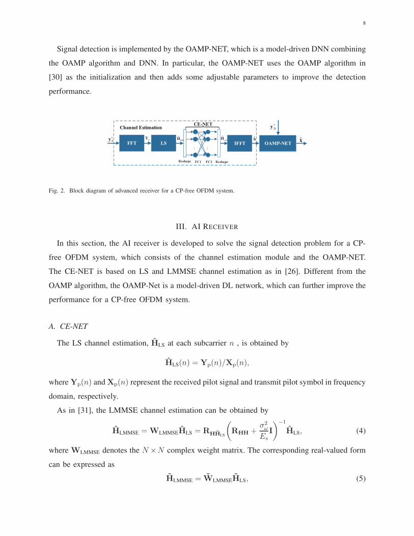
The AI receiver module is shown in Fig. 2, including channel estimation and an OAMP-NET.
The channel estimation is developed from the channel estimation subnet as in ComNet [26]
because of its predictability and accuracy. The input of channel estimation, ytp, is first converted
into the frequency domain by FFT. Then the block, LS, performs the least-squares (LS) channel
estimation to obtain HLS, which initializes the subsequent neural network to generate more
accurate channel estimation, Hout.
8
Signal detection is implemented by the OAMP-NET, which is a model-driven DNN combining
the OAMP algorithm and DNN. In particular, the OAMP-NET uses the OAMP algorithm in
[30] as the initialization and then adds some adjustable parameters to improve the detection
performance.
...
...
FC1 FC2Reshape
t
Py
t
Dy
FFT LS OAMP-NETIFFT�xY
p�
LSH �H
out�h
Reshape
Channel EstimationCE-NET
Fig. 2. Block diagram of advanced receiver for a CP-free OFDM system.
III. AI RECEIVER
In this section, the AI receiver is developed to solve the signal detection problem for a CP-
free OFDM system, which consists of the channel estimation module and the OAMP-NET.
The CE-NET is based on LS and LMMSE channel estimation as in [26]. Different from the
OAMP algorithm, the OAMP-Net is a model-driven DL network, which can further improve the
performance for a CP-free OFDM system.
A. CE-NET
The LS channel estimation, HLS at each subcarrier n , is obtained by
HLS(n) = Yp(n)/Xp(n),
where Yp(n) and Xp(n) represent the received pilot signal and transmit pilot symbol in frequency
domain, respectively.
As in [31], the LMMSE channel estimation can be obtained by
HLMMSE = WLMMSEHLS = RHHLS
(
RHH +σ2ω
EsI
)−1
HLS, (4)
where WLMMSE denotes the N ×N complex weight matrix. The corresponding real-valued form
can be expressed as
HLMMSE = WLMMSEHLS, (5)

9
where
HLMMSE =
Re{HLMMSE}Im{HLMMSE}
, HLS =
Re{HLS}Im{HLS}
,
and
WLMMSE =
Re{WLMMSE} Im{WLMMSE}Im{WLMMSE} Re{WLMMSE}
.
As shown in Fig. 2, the channel estimation module consists of FFT, LS, CE-NET, and IFFT.
Then, HLS is used by the CE-NET to generate more accurate Hout through an one-layer DNN
with specially designed initial weights. The CE-NET is a simple neural network with one input
layer and one output layer. The weights are initialized by using the real-valued LMMSE channel
estimation weight, WLMMSE. The biases are initially set as zero. The input of the CE-NET is
real-value HLS, which has 2N neutrons. The number of neurons in the output layer is also 2N .
These output neurons have no activation function. The CE-NET is trained by minimizing the
the ℓ2 loss between predictions and known channel samples by using a specific optimizer. The
weights and bias are updated by back propagation algorithm [32] during the training process.
B. OAMP-NET
Recently, iterative detectors based on approximate message passing (AMP) have been proposed
for MIMO detection [13], [30], [33] since they have low complexity and are easily implemented
in practice. Therefore, we will apply the OAMP algorithm for signal detection in a CP-free
OFDM system. The interference from the previous OFDM blocks, corresponding to the second
term in (2), must be eliminated to apply the OAMP algorithm. As depicted in Fig. 2, the receiver
acquires the CSI, h, by CE-NET. After removing the residual IBI, the received signal can be
expressed as
y = y−Aq−1 (6)
= JFHu+Aq−1 −Aq−1 +w
= Hu+w′,
where J and A are derived by the estimated h, H = JFH , and w′ = Aq−1 − Aq−1 +w with
a variance of σ2ω′ . The OAMP-NET is then performed to detect the transmitted OFDM block.
As the OAMP-NET only addresses real-valued variables, the complex-valued OFDM system is
converted into the corresponding real-valued one before OAMP detection as (5) in Section III.A.

10
To simplify the symbolic notations, new real-version variances are omitted and the complex-
version variances represent the real ones below. For example, the real version of H can be noted
as H, but we continue use H to represent H.
Algorithm 1 OAMP Algorithm for CP-free OFDM
Input: y: the received signal in time domain;
SNR: Signal to Noise Ratio (dB);
Output: b: recovered signal
1: initialize: L = 10, β = 0.5, υ20 = 0, u1 = 0
2: acquire the h in real time by the trained CE-NET
3: compute J,A according to h
4: obtain the noise power by (3)
5: attain y, H, w′ by (6)
6: for l = 1 to L do
7: execute OAMP algorithm:
rl = ul +Pl(y −Hul) (7)
υ2l =
‖y−Hul‖2 −Mσ2ω′
tr(HHH)(8)
υ2l = (1− β)υ2
l−1 + βυ2l (9)
τ 2l =1
2Ntr(BlB
Hl )υ
2l +
1
4Ntr(PlP
Hl )σ
2ω′ (10)
ul+1 = E{u|rl, τl} (11)
8: l = l + 1
9: end for
10: demodulate uL+1 to obtain b.
The OAMP-based detector [30] can be summarized as Algorithm 1. In (7), l indicates the
index of the iteration times. According to [13], the optimal matrix Pl is given by
Pl =2N
tr(PlH)Pl (12)
11
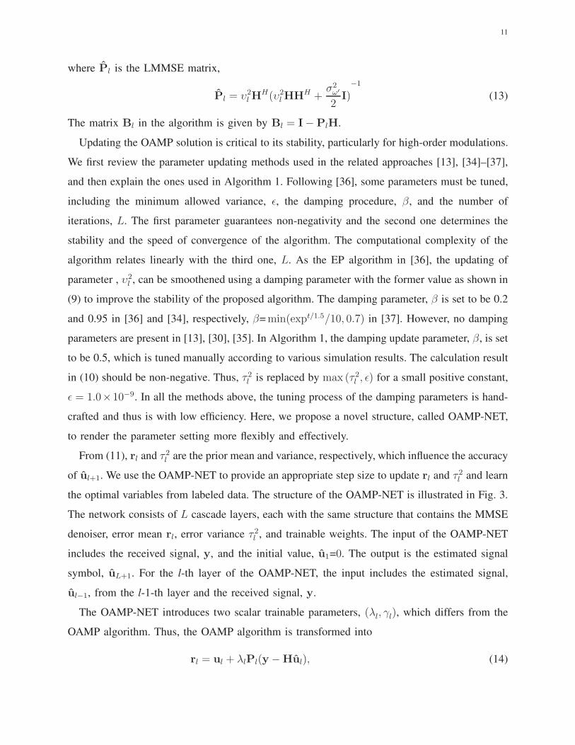
where Pl is the LMMSE matrix,
Pl = υ2l H
H(υ2l HHH +
σ2ω′
2I)
−1
(13)
The matrix Bl in the algorithm is given by Bl = I−PlH.
Updating the OAMP solution is critical to its stability, particularly for high-order modulations.
We first review the parameter updating methods used in the related approaches [13], [34]–[37],
and then explain the ones used in Algorithm 1. Following [36], some parameters must be tuned,
including the minimum allowed variance, ǫ, the damping procedure, β, and the number of
iterations, L. The first parameter guarantees non-negativity and the second one determines the
stability and the speed of convergence of the algorithm. The computational complexity of the
algorithm relates linearly with the third one, L. As the EP algorithm in [36], the updating of
parameter , υ2l , can be smoothened using a damping parameter with the former value as shown in
(9) to improve the stability of the proposed algorithm. The damping parameter, β is set to be 0.2
and 0.95 in [36] and [34], respectively, β=min(expt/1.5/10, 0.7) in [37]. However, no damping
parameters are present in [13], [30], [35]. In Algorithm 1, the damping update parameter, β, is set
to be 0.5, which is tuned manually according to various simulation results. The calculation result
in (10) should be non-negative. Thus, τ 2l is replaced by max (τ 2l , ǫ) for a small positive constant,
ǫ = 1.0×10⁻⁹. In all the methods above, the tuning process of the damping parameters is hand-
crafted and thus is with low efficiency. Here, we propose a novel structure, called OAMP-NET,
to render the parameter setting more flexibly and effectively.
From (11), rl and τ 2l are the prior mean and variance, respectively, which influence the accuracy
of ul+1. We use the OAMP-NET to provide an appropriate step size to update rl and τ 2l and learn
the optimal variables from labeled data. The structure of the OAMP-NET is illustrated in Fig. 3.
The network consists of L cascade layers, each with the same structure that contains the MMSE
denoiser, error mean rl, error variance τ 2l , and trainable weights. The input of the OAMP-NET
includes the received signal, y, and the initial value, u1=0. The output is the estimated signal
symbol, uL+1. For the l-th layer of the OAMP-NET, the input includes the estimated signal,
ul−1, from the l-1-th layer and the received signal, y.
The OAMP-NET introduces two scalar trainable parameters, (λl, γl), which differs from the
OAMP algorithm. Thus, the OAMP algorithm is transformed into
rl = ul + λlPl(y−Hul), (14)

12
l-th layer L-th layer
MMSE+
1-th layer
Ty
+
y
1u
2u
y y yy
ul +1
ul
uL
y
1uL+
rl
ul
Wl ll
2
lt
2
ln
yy
+1ul
MMSE+
Ty
+
rl
rull
Wl lWWl
2
lt
2
ln
yy
+1ul
Wl lWll ll lH
Fig. 3. Structure of the OAMP-NET.
υ2l =
‖y −Hul‖2 −Mσ2ω′
tr(HHH), (15)
τ 2 =1
2Ntr(DlD
Hl )υ
2l +
γ2l
4Ntr(PlP
Hl )σ
2ω′ , (16)
ul+1 = E{u|rl, τl}, (17)
where Dl = I − γlPlH. Two trainable variables in each layer, (λl, γl), are introduced in the
OAMP-NET, which is the difference from the TISTA in [28]. If λl = γl, the OAMP-NET
is simplified to the TISTA. The transmitted symbol, u, is obtained from the real alphabet
modulation set, A = {a1, ..., am, ..., a√M} and the corresponding posterior mean estimator,
E{u|rl, τl}, in (17) for each element of ul+1 is given by
E{un|rnl , τl}=
∑
am∈A amN (am; rnl , τ
2l )
∑
am∈AN (am; rnl , τ2l )
. (18)
Different from the OAMP algorithm, the damping parameter β is removed from OAMP-NET.
Each layer in Fig. 3 contains only two adjustable variables (λl, γl). Therefore, the total number
of trainable variables is equal to 2L if there are L layers. Furthermore, the number of trainable
variables of the OAMP-NET is independent of the number of subcarriers N in OFDM and is
only related to by the number of layers L. This feature is advantageous for an OFDM system
with many subcarriers. The trainable variables of the OAMP-NET are much fewer than those of
FC-DNN [25] and ComNet [26]. Moreover, convergence, stability, and speed can be improved
during training.

13
C. Complexity Analysis
The complexity of the model-based receiver and the AI-aided receiver is compared in Table I
in terms of the number of floating-point multiplication-adds (FLOPs), the number of parameters,
and running time required to complete a single-forward pass of one OFDM block. LS+OFDM
represents the traditional LS channel estimation and expert OFDM detection which is the result
of YD divided by estimated channel HLS. YD represents the received signal in frequency
domain. Traditional LMMSE channel estimation and expert OFDM detection is denoted by
LMMSE+OFDM. All algorithms listed before CE-NET+OAMP in Table I are model-based,
whereas others are AI-aided. CE-NET+OAMP indicates that the CSI is obtained by CE-NET
and the signal is detected by the OAMP algorithm. Our proposed AI-aided receiver is designated
as AI receiver and other AI-aided receivers are denoted as [25] and ComNet [26].
For the OAMP algorithm and the OAMP-NET, complexity is dominated by the computation
of the covariance matrix in (13) whose complexity is O(n3L). The number of FLOPs of OAMP
algorithm is approximately 1.05 × 10⁷ (L = 5). From Fig. 3, the total number of trainable
variables is equal to 2L, as each layer of the OAMP-Net contains only two adjustable variables
(λl, γl).
From Table I, the LMMSE+OAMP requires the largest number of FLOPs and the LS+OFDM
requires the least. For the model-based receivers, the number of FLOPs and running time tend to
increase from topmost item downwards, in which the LS+OFDM needs 3.3× 10⁻³ s, whereas
LMMSE+OAMP needs 5.6× 10⁻² s . There is a gap between the FLOPs of LMMSE and CE-
NET because LMMSE needs to compute the inverse matrix as in (4) while CE-NET has been
trained. Therefore, the difference of the FLOPs between LMMSE+OAMP and CE-NET+OAMP
is approximately 1.6 million FLOPs. Obviously, our proposed AI receiver demands the same
number of FLOPs as LS+OAMP as the AI receiver does not change the structure of the OAMP
algorithm and merely introduces 6.5× 10⁻² Mbytes in training parameters. For the DNN, the
number of parameters is used to measure the complexity. Note that the FC-DNN has the most
parameters followed by ComNet and then by our AI receiver has the least. On the contrary,
the running time of the AI receiver is much more than that of FC-DNN and ComNet since
the computation of the inverse matrix in the OAMP-NET structure consumes lots of time. The
running time of the model-driven and model-based receivers are generally a little longer than
those of completely data-driven AI-aided receivers. The time consumption is influenced not

14
only by FLOPs but also the limitations of intensity and roofline [9], the platform, cache size,
and realization method. The presented running time of the model-based methods and the AI
receiver are computed by MATLAB, whereas the FC-DNN and ComNet are tested on Python
with parallelization.
TABLE I
COMPLEXITY COMPARISON FOR PROPOSED SCHEMES AND COMPETING METHODS
Algorithm FLOPs #parameter Time
LS+OFDM 768 × 3.3 × 10−3 s
LMMSE+OFDM 1.6M × 1.3 × 10−2 s
LS+OAMP 10.5M × 5.0 × 10−2 s
LMMSE+OAMP 12.1M × 5.6 × 10−2 s
CE-NET+OAMP 10.5M 0.065MBytes 5.1 × 10⁻² s
AI receiver 10.5M 0.065MBytes 5.1 × 10⁻² s
FC-DNN × 9.30MBytes 1.2 × 10⁻⁶ s
ComNet × 2.4MBytes 7.2 × 10⁻⁶ s
IV. SIMULATION RESULTS AND DISCUSSIONS
This section presents simulated results, which provide guideline for the OTA test of AI-aided
receiver for a CP-free OFDM system.
A. Parameters Setting
A CP-free OFDM system is with 64 subcarriers in our simulation. To estimate the channel,
different types of pilots are inserted into the OFDM blocks according to the speed of channel
variation. For the quasi-static fading channels that changes after passing several OFDM blocks,
the pilot OFDM block and subsequent several data OFDM blocks usually form a frame. In our
simulation, one pilot OFDM block and one data OFDM block constitute one frame as shown in
Fig. 4(a) for simplicity. For the fasting fading channels that changes between adjacent OFDM
blocks, comb type pilots are uniformly distributed within each OFDM block as in Fig. 4(b).
To verify the robustness of the proposed algorithms, two types of channel models are simulated:
the wireless world initiative new radio II (WINNNERII) [38] and Stanford University Interim
(SUI) [31]. In the WINNNERII channel, the carrier frequency is 2.6 GHz, the number of paths

15
is 24, and typical urban channels with max delay 16 samples are used, which is also consistent
with the channel models in [25] and [26]. For the SUI channel, the delay spreads are [0, 4, 10]
and the corresponding average powers of the three paths are [0 dB, -5 dB, -10 dB]. The types
of modulation are 16-QAM and 64-QAM.
Fre
qu
ency
Time
Fre
qu
ency
Pilot
Data
Time(a) (b)
Fig. 4. Pilot arrangement of the quasi-static fading channels and the fast fading channels. (a) Continuous pilot arrangement for
the quasi-static fading channels. (b) Comb type pilot arrangement of the fast fading channels.
The CE-NET and OAMP-NET are trained by minimizing the cost between predictions and
actual labels by using the adaptive moment estimator (Adam) optimizer. The learning rate is set
to 0.001. We select the ℓ2 loss as the cost function. In the CE-NET, the training and testing sets
contain 3, 000, 000 and 1, 000, 000 channel samples, respectively. The batch size and epochs are
set to 50 and 2,000, respectively. The CE-NET and the OAMP-NET are trained separately. After
finishing the training of the CE-NET, the OAMP-NET is trained by known data symbols with
10, 000 epochs. The OAMP-NET has 10 layers. At each epoch, the training and development sets
both contain 1,000 samples, respectively. We continue generating the test data for the OAMP-
NET until the number of bit errors exceeds 1,000. The training parameters of the CE-NET and
the OAMP-NET are summarized in Tables II and III, respectively.
The following naming conventions are employed to concisely present the performance:
• (XX dB): obtained by training a neural network with the received data under SNR = XX
dB, but predicted the results among different SNRs;
• (ALL dB): indicates that the neural network is trained under the matched SNR value. For
example, the predicted value under SNR = 25 dB is obtained when the neural network is
also trained under SNR = 25 dB;
• OAMP-NET(xxQAM, XXdB): the specific OAMP-NET is trained under xx-QAM with XX
dB and trained network structure is used to predict the results of other situations;

16
TABLE II
TRAINING PARAMETERS OF CE-NET.
Parameter Value
SNR 5-40 dB
Loss function ℓ2
Batch size 50
Epoch 2000
Initial learning rate 0.001
Optimizer Adam
TABLE III
TRAINING PARAMETERS OF OAMP-NET.
Parameter Value
SNR 5-40 dB
Loss function ℓ2
Batch size 1000
Epoch 10000
Initial learning rate 0.001
Optimizer Adam
• 16 pilot: comb pilots with 16 pilots applied;
• 64 pilot: continuous pilots with 64 pilots applied;
• S: the SUI channel;
• W: the WINNERII channel; and
• S/W: the SUI or WINNERII channel.
For example, OAMP-NET(64QAM, ALLdB) indicates that the specific OAMP-NET is trained
under 64-QAM with a SNR and the trained network structure is used to predict the results of
other situations with matched SNR. If no special illustrations are present, then the continuous
pilots, the ALLdB and WINNERII channels, are applied in the simulation.
B. Performance Analysis of CE-NET
The purpose of the CE-NET is to acquire accurate CSI information, which is beneficial for
the subsequent signal detection utilizing OAMP-NET and adopting high-order QAM modulation.

17
5 10 15 20 25 30 35 40
SNR(dB)
-50
-45
-40
-35
-30
-25
-20
-15
-10
-5
0
MS
E(d
B)
LSLMMSECE-NET(20dB)CE-NET(40dB)CE-NET(ALLdB)LMMSEwCP
(a) Continuous pilots on the WINNERII channel
5 10 15 20 25 30 35 40
SNR(dB)
-50
-45
-40
-35
-30
-25
-20
-15
-10
-5
0
MS
E(d
B)
LSLMMSECE-NET(20dB)CE-NET(40dB)CE-NET(ALLdB)LMMSEwCP
(b) 16 comb pilots on the WINNERII channel
Fig. 5. MSE curves of CE-NET and traditional methods in different conditions. (a) continuous pilots on WINNERII channel.
(b) comb pilots on WINNERII channel.
With only a single training, the CE-NET can adapt to time-varying channels.
Fig. 5(a) shows the MSE performance of different channel estimation methods applied to
the WINNERII channel. As shown in Fig. 5(a), the MSE curves of CE-NET(20 dB) present a
saturation property similar to the traditional channel estimation methods of LS and LMMSE.
However, the CE-NET(40 dB) rectifies the nonlinear effects and has better performance than
LMMSE with sufficient CP when SNR is higher than 25 dB, which suggests its effectiveness and
feasibility. Furthermore, the MSE of CE-NET(ALLdB) is lower than LMMSE with sufficient
CP. Compared with the CE-NET(ALLdB), CE-NET(40 dB) has minimal performance loss but
endures less training complexity.
As shown in Fig. 5(b), the CE-NET(20 dB) is more robust than that of CE-NET(40 dB)
which works effectively in low SNR. In addition, CE-NET(ALLdB) entails more training cost
but achieves only little gain. Therefore, in this scenario, we choose the weights and bias for the
CE-NET trained under 20 dB. Note also that the performance of the CE-NET working in comb
pilots is much better than the traditional LS and LMMSE and obtain approximately 10 dB gain
when SNR = 30 dB. In addition, the biggest gap between CE-NET(20 dB) and LMMSE with
sufficient CP called LMMSEwCP in the Fig. 5(b) is approximately 7 dB at SNR = 40 dB, but
the least difference is lower than 1 dB at SNR = 20 dB. Overall, the CE-NET is effective and
robust as it significantly outperforms LS and LMMSE.
18
For the SUI channels, the channel estimation performance is similar with that of the WIN-
NERII channels, which also suggests the effectiveness of the CE-NET. Compared with the
WINNERII channels, the difference of the SUI channels lies in lower delay and fewer paths. By
applying the AI receiver to the new channel, the adaptation and flexibility for different channel
environments have been demonstrated from the above discussion.
C. Performance of OAMP-NET
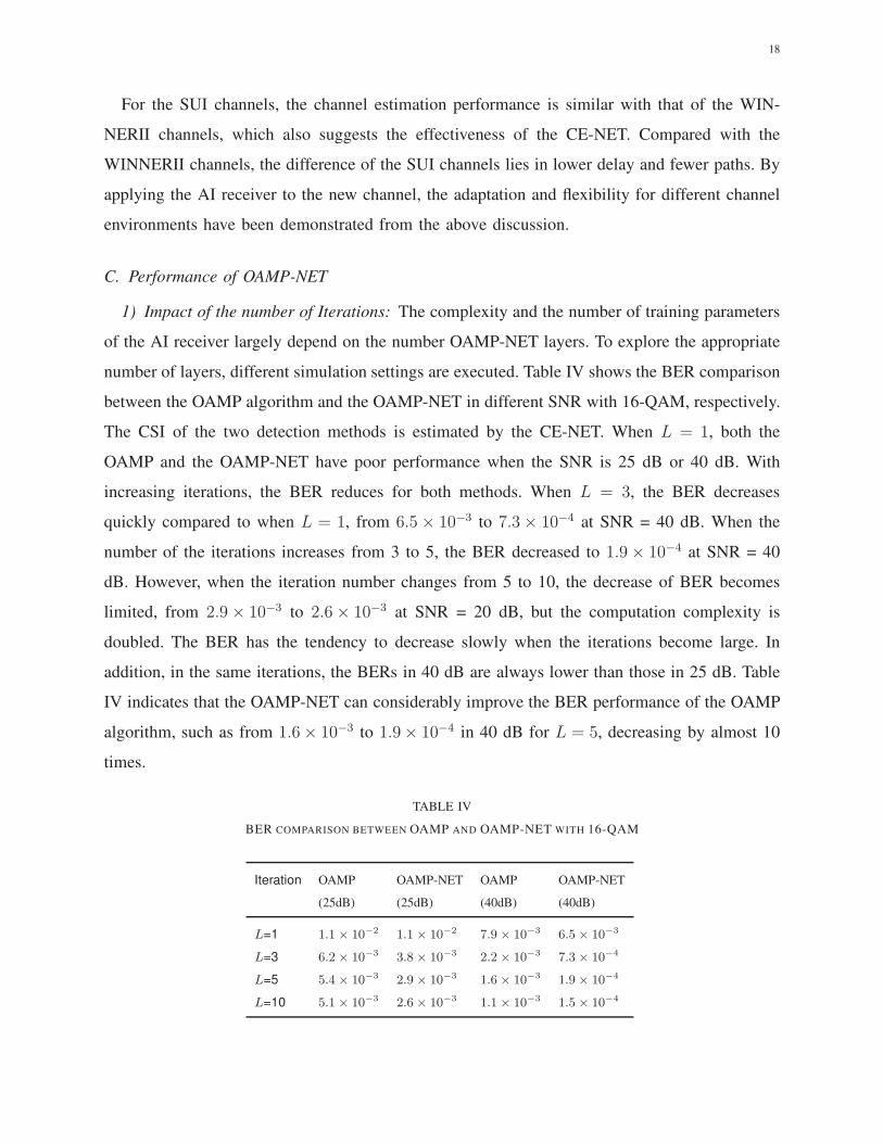
1) Impact of the number of Iterations: The complexity and the number of training parameters
of the AI receiver largely depend on the number OAMP-NET layers. To explore the appropriate
number of layers, different simulation settings are executed. Table IV shows the BER comparison
between the OAMP algorithm and the OAMP-NET in different SNR with 16-QAM, respectively.
The CSI of the two detection methods is estimated by the CE-NET. When L = 1, both the
OAMP and the OAMP-NET have poor performance when the SNR is 25 dB or 40 dB. With
increasing iterations, the BER reduces for both methods. When L = 3, the BER decreases
quickly compared to when L = 1, from 6.5× 10⁻³ to 7.3× 10⁻⁴ at SNR = 40 dB. When the
number of the iterations increases from 3 to 5, the BER decreased to 1.9× 10⁻⁴ at SNR = 40
dB. However, when the iteration number changes from 5 to 10, the decrease of BER becomes
limited, from 2.9× 10⁻³ to 2.6× 10⁻³ at SNR = 20 dB, but the computation complexity is
doubled. The BER has the tendency to decrease slowly when the iterations become large. In
addition, in the same iterations, the BERs in 40 dB are always lower than those in 25 dB. Table
IV indicates that the OAMP-NET can considerably improve the BER performance of the OAMP
algorithm, such as from 1.6× 10⁻³ to 1.9× 10⁻⁴ in 40 dB for L = 5, decreasing by almost 10
times.
TABLE IV
BER COMPARISON BETWEEN OAMP AND OAMP-NET WITH 16-QAM
Iteration OAMP OAMP-NET OAMP OAMP-NET
(25dB) (25dB) (40dB) (40dB)
L=1 1.1× 10⁻²
1.1× 10⁻²
7.9× 10⁻³
6.5× 10⁻³
L=3 6.2× 10⁻³
3.8× 10⁻³
2.2× 10⁻³
7.3× 10⁻⁴
L=5 5.4× 10⁻³
2.9× 10⁻³
1.6× 10⁻³
1.9× 10⁻⁴
L=10 5.1× 10⁻³
2.6× 10⁻³
1.1× 10⁻³
1.5× 10⁻⁴

19
2) Performance for the WINNERII and SUI channels with perfect CSI: The BER curves of
the OAMP-NET and the competitive methods in the CP-free case with 64-QAM and 16-QAM
are shown in Fig. 6. In the simulation below, the perfect CSI is employed for signal detection
at the receiver. LowBound indicates that the maximum likelihood (ML) detector is used in the
conventional CP-OFDM system.
In Fig. 6(a), the traditional OFDM detection does not satisfy the orthogonal property of
subcarriers because of the effect of CP removal. Thus, the method exhibits poor performance.
On the one hand, the BER of the OAMP-NET is lower than that of the RISIC algorithm in
[3]. On the other hand, the OAMP-NET can remarkably improve the performance of the OAMP
algorithm. These findings indicate the superiority of the OAMP-NET by introducing only a few
parameters. In addition, the gap between LowBound and the OAMP-NET is extremely small
when the SNR is lower than 30 dB. However, the gap becomes slightly larger when the SNR is
higher than 30 dB.
5 10 15 20 25 30 35 40
SNR(dB)
10-4
10-3
10-2
10-1
100
BE
R
OFDMRISICOAMPOAMP-NETLowBound
(a) 64-QAM on WINNERII channel.
5 10 15 20 25 30 35 40SNR(dB)
10-4
10-3
10-2
10-1
100
BE
R
OFDMRISICOAMPOAMP-NETLowBound
(b) 16-QAM on WINNERII channel.
Fig. 6. BER curve of OAMP-NET and competitive methods under the CP-free case with 64-QAM and 16-QAM on WINNERII
channel. (a) 64-QAM. (b) 16-QAM.
Figure 6(b) shows the BER performance for 16-QAM modulation in the WINNERII channel.
Unlike that with 64-QAM, the BER of the OAMP algorithm for 16-QAM is higher than that
of the RISIC algorithm when the SNR is over 25 dB. However, the BER of the OAMP-NET
is much lower than that of the RISIC algorithm since the parameters (λl, γl) are tuned in the
OAMP-NET in each layer, thereby resulting in a flexible network. In addition, the gap between

20
the OAMP-NET and LowBound is smaller than that with 64-QAM. When the SNR is below 20
dB, the BER of the OAMP-NET approaches the performance of LowBound. With the mounting
SNR, the gap becomes a little larger but much less than that with 64-QAM. In summary, the
OAMP-NET exhibits excellent BER performance compared with the existing algorithms and
is close to the performance limit of an OFDM system with sufficient CP for 16-QAM and 64-
QAM. However, the performance of the OAMP-NET with 16-QAM is closer to the performance
limit than that with 64-QAM. Therefore, there is still a room to improve a CP-free OFDM with
64-QAM modulation.
The BER performance of the relevant algorithms under the SUI channel is similar to those
under the WINNERII counterpart. Different from the WINNERII channel, the BER of the OAMP
algorithm for 16-QAM is always lower than that of the RISIC algorithm.
D. Robustness Analysis
1) 16 pilot: When the comb pilots are applied, the MSE of CE-NET has a remarkable gap
with the continuous pilots as Fig. 5(b) shows. Fig. 7 depicts the BER curves of the OAMP and
the OAMP-NET in the case of 16 comb pilots on the WINNERII channel.
Fig. 7(a) indicates that the model-based algorithm, LMMSE+OAMP, does not work as the
LMMSE channel estimation in the comb pilots without CP. However, by introducing a neural
network, CE-NET+OAMP outperforms LMMSE+OAMP even if both of them have the tendency
to be saturated. In Fig. 7(a), the BER can be greatly decreased by applying the OAMP-NET.
The BER performance with 16-QAM is similar to that with 64-QAM. The difference from 64-
QAM is that the LMMSE+OAMP and CE-NET+OAMP have more severe amplitude fluctuation
and bigger performance degradation when the SNR is more than 25 dB because the damping
exploded and the actual noise does not match the estimated noise owing to the greater noise
introduced by the first term of (7). Clearly, the OAMP-NET is superior to the OAMP algorithm
as the former needs no hand-crafted damping parameters but can prevent damping exploration.
Overall, the performance of the OAMP-NET in the case of imprecise channel estimation verifies
its robustness.
2) Adaptation of OAMP-NET: To test the robustness of the OAMP-NET, the trained param-
eters of 64-QAM with 40 dB in the WINNERII channels is applied to other SNRs of 64-QAM
and 16-QAM, as shown in Fig. 8. In Fig. 8(a), the BER performances of the OAMP, the OAMP-
NET training under matched SNR, and OAMP-NET training under 40 dB in the WINNERII

21
5 10 15 20 25 30 35 40
SNR(dB)
10-4
10-3
10-2
10-1
100
BE
R
LMMSE+OAMPCE-NET+OAMPCE-NET+OAMP-NETLMMSE+OFDMwCP
(a) 16 comb pilots with 64-QAM.
5 10 15 20 25 30 35 40
SNR(dB)
10-4
10-3
10-2
10-1
100
BE
R
LMMSE+OAMPCE-NET+OAMPCE-NET+OAMP-NETLMMSE+OFDMwCP
(b) 16 comb pilots with 16-QAM.
Fig. 7. BER curve of OAMP and OAMP-NET with 16 comb pilots on the WINNERII channel. (a) 64-QAM. (b) 16-QAM.
5 10 15 20 25 30 35 40
SNR(dB)
10-4
10-3
10-2
10-1
100
BE
R
OAMP(64QAM)OAMP-NET(64QAM, ALLdB)OAMP-NET(64QAM, 40dB)
(a) Robustness with 64-QAM.
5 10 15 20 25 30 35 40SNR(dB)
10-4
10-3
10-2
10-1
100
BE
R
OAMP(16QAM)OAMP-NET(16QAM, ALLdB)OAMP-NET(64QAM, 40dB)
(b) Robustness with 16-QAM.
Fig. 8. BER curve of OAMP-NET with different training cost on the WINNERII channel. (a) 64-QAM. (b) 16-QAM.
channels are depicted. When SNR is lower than 15 dB, the performance of the OAMP-NET with
40 dB is same as that of the matched SNR performance. With increasing SNR, the performance
experiences only minimal loss. In addition, the OAMP-NET with 40 dB performs much better
than the OAMP algorithm and shows only a little degradation compared with ALLdB, which
suggests that OAMP-NET has strong robustness and can adapt to different SNRs with 64-QAM.
To further verify the robustness, the trained parameters of 64-QAM with 40 dB are applied to

22
16-QAM in Fig. 8(b). Form the figure, the OAMP-NET of 64-QAM with 40 dB can work well
on 16-QAM. On the one hand, the OAMP-NET of 64-QAM with 40 dB performs better than
the OAMP algorithm with 16-QAM when the SNR is higher than 15 dB. On the other hand,
the performance has little gap with the totally matched OAMP-NET, namely OAMP-NET of
16-QAM with ALLdB. In summary, the OAMP-NET trained in higher modulation mode can
adapt to a lower one, which is beneficial for modulation handover.
Table V shows the BER of the OAMP-NET trained with 40 dB in different conditions,
including the channel and modulation modes, where OAMP-NET refers to the BER obtained
under corresponding matched conditions, OAMP-NET1 and OAMP-NET2 denote the specific
OAMP-NETs trained under 16-QAM and under 64-QAM with 40 dB in the WINNERII channels,
respectively. OAMP-NET1 results suggest that all BERs are lower than the OAMP algorithm.
The phenomenon indicates that the OAMP-NET1 is not only valid for the WINNERII channels,
but also adapt to the SUI channels as the latter is simpler than the former. However, the BERs
of OAMP-NET1 are slightly higher than those of the OAMP-NET, which is reasonable due to
the total match for the OAMP-NET. Similar results can be found for the OAMP-NET2. For the
SUI channels with 64-QAM, OAMP-NET2 is more precise than OAMP-NET1. Conversely, for
the SUI channels with 16-QAM, OAMP-NET1 is more accurate than OAMP-NET2.
TABLE V
BER COMPARISON BETWEEN OAMP AND OAMP-NET
Iteration 64-QAM 16-QAM 64-QAM 16-QAM
(W) (W) (S) (S)
OAMP 0.010677 0.002131 0.010219 0.002922
OAMP-NET 0.003458 0.000277 0.003654 0.000148
OAMP-NET1 0.0045 0.000277 0.0089 0.00043
OAMP-NET2 0.003458 0.0008989 0.0075 0.0012
E. Capacity Analysis
Fig. 9 compares capacities of the AI receiver and traditional OFDM with sufficient CP in
different scenarios, including continuous pilots and comb pilots, as well as the WINNERII and
SUI channels. The bandwidth in the simulation is 20 MHz. The capacity of the AI receiver
with comb pilots in the WINNERII or SUI channels performed best for all scenarios because

23
5 10 15 20 25 30 35 40SNR(dB)
2
3
4
5
6
7
8
9
10
Cap
acity
(bps
)
×107
AI receiver(S/W,16pilot)OFDMwCP(S,16pilot)OFDMwCP(W,16pilot)AI receiver(S/W,64pilot)OFDMwCP(S,64pilot)OFDMwCP(W,64pilot)
Fig. 9. Capacity comparison between AI receiver and traditional OFDM with sufficient CP in difference scenarios including
the 64pilot and 16pilot, and the WINNERII and SUI channels.
the CP is removed from an OFDM block and comb pilots occupy less resource blocks of
OFDM. Therefore, the spectrum efficiency is relatively high and the amount of transmission
data are significantly improved. It also accounts for the fact that the curves of the comb pilots
are obviously beyond those of using continuous ones. Our proposed AI receiver can work well
in these scenarios, which indicates that the AI receiver has significant spectrum efficiency.
Fig. 10 compares the BER performance of the AI receiver with other AI-aided methods,
including the FC-DNN studied by [25] and ComNet of [26]. FC-DNN become saturated when
the SNR is higher than 25 dB, whereas the ComNet and the AI receiver perform better in
resolving the CP-free issue, which suggests the advantages of a model-driven DNN. Compared
with those of the ComNet, the BER of the AI receiver reduces considerably from 2.0× 10⁻² to
6.0× 10⁻³ when SNR equals 30 dB. Therefore, the OAMP-NET has the ability to recover raw
bit stream more accurately.
V. OTA TEST AND RESULT DISCUSSION
Apart from simulation, we have also developed a prototyping system to verify the effectiveness
and feasibility of the proposed algorithms in real channel environments. In this subsection, we
compare the performance of the AI receiver with the FC-DNN and ComNet receivers in OTA
tests.

24
5 10 15 20 25 30 35 40
SNR(dB)
10-4
10-3
10-2
10-1
100
BE
R
FC-DNNComNetCE-NET+OAMP-NETLowBound
Fig. 10. BER performance of the AI receiver and other AI-aided methods with 64-QAM.
A. System Setup
As shown in Fig. 11, the real testing scenario includes a transmitter and a receiver of OTA,
which offers processing and transmission of OFDM with 64 subcarriers. For simplicity, the
modulation mode of QPSK is applied in the real scenario. In [39], a novel 5G RaPro system is
proposed to deploy FPGA-privileged modules on software defined radio (SDR) platforms. Such
architecture has been proven to be flexible and scalable by deploying a multi-user full-dimension
MIMO prototyping system.
Transmitter of OTA Test Receiver of OTA Test
Fig. 11. Real testing scenario consisting of transmitter and receiver.
We use the RaPro system as our testbed to evaluate the OTA performance of the AI receiver
in a CP-free OFDM as found in [27]. To implement a CP-free OFDM communication system
with the AI receiver, we employ two SDR nodes of the universal software radio peripheral

25
reconfigurable I/O (USRP-RIO) series manufactured by National Instruments. Each SDR node
includes one RF transceiver of 20 MHz bandwidth and a programmable FPGA responsible for
distributed signal processing, such as the reciprocity calibration or OFDM (de)modulation [39].
Fig. 12 illustrates the OFDM block structure of the CP-free OFDM system. From Fig. 12, each
OFDM block contains 128 subcarriers, where 64 subcarriers are effective for transmitting pilot
symbols or data symbols, 63 subcarriers are used as the guard band, and a subcarrier is the
direct current (DC) offset. Each frame consists of one pilot OFDM block and one data OFDM
block, which is the same as the simulation setting.
OFDM Block
31
Protection
DC
32
Effective carrier
32
Effective carrier
32
Protection
Fig. 12. Structure of the OFDM blocks in a CP-free real testing scenario.
For the transmitter in the OTA test, 64 subcarriers and 128 binary numbers as the QPSK
are applied. We choose the first 16 binary numbers by sequentially inserting 216 data from
0000000000000000 to 1111111111111111, which can be regarded as labels to assess the BER
for the real channel environment. Then, the pilot symbols are inserted and packaged into a
frame together with data symbols. Due to out-of-band emission, bandwidth protection requires
the additional guard band and DC offset according to the designed OFDM block. Next, the IFFT
is performed and the frame head is added to detect the OFDM blocks precisely. Wireless signals
are transmitted by an USRP-RIO through a RF antenna, whose center frequency is adjustable
in the range of 1.2-6 GHz. The channel environment is indoors and the distance between the
transmitted RF antenna and received RF antenna is 5 meters. The receiver in the OTA test first
conducts frame detection, then perform FFT and estimates the CSI, subsequently transforming
the CSI from the frequency domain to the time domain. Finally, the data signals are transmitted
to our OAMP-NET to obtain the estimated transmitting bits, just as Fig. 2 shows.
The development of the proposed AI receiver can be divided into two phases, the training and
the detecting phases. The training phase is developed in Python based on TensorFlow by relying
on the GPUs’ powerful computing ability. OTA data captured by USRP-RIO is used to train the

26
weights and biases of the DNN via the back propagation algorithm. These parameters are stored
into a file after training and provided for the detecting phase. In the detecting phase, forward
propagation is implemented in TensorFlow, with the stored parameters as the initialization value
of the weight matrices and bias vectors.
B. Experimental Results
We choose two different scenarios to test our AI receiver. Scenario 1 is the fixed indoor
scenario, where the transmitter is 5 meters away from the receiver in the same room with fixed
obstacles, windows, and walls. Scenario 2 is the changing indoor scenario, in which the only
difference with Scenario 1 is the presence of people walking around. Both two scenarios are
relatively simple because of limited transmission distance, reflectors, and scatters. Moreover, the
corresponding real channels are similar to the exponential power delay profile defined in IEEE
802.11b [31], which is denoted as the exponential (EXP) channel. Therefore, our proposed AI
receiver, FC-DNN and ComNet are trained offline under the EXP channel model to perform the
OTA test using the same SNR and by a specific transmitter antenna gain.
The conventional LS+OFDM method is used as the baseline. In Scenario 1 in Table VI, our
AI receiver method achieves similar BER performance with LS+OFDM and slightly outperforms
the other two AI-aided OFDM receivers, whereas the FC-DNN receiver is slightly better than
the ComNet receiver. The main reason for such outcomes is that this OTA scenario has limited
transmission distances and obstacles, which leads to simple channel realizations. In Scenario
2, we establish a more complex channel environment by increasing the moving scatters. Test
results show that the LS+OFDM, FC-DNN, and ComNet receivers have poor performance in the
OTA test. Our AI-aided OFDM receiver shows its advantage in the abovementioned complex
real channels because it is designed to deal with nonlinear and complex channel conditions by
using nonlinear functions.
TABLE VI
BER OF AI RECEIVERS FOR OTA TEST
LS+OFDM FC-DNN ComNet OAMP-NET
Scenario 1 3.9× 10⁻⁴
5.4× 10⁻⁴
7.8× 10⁻⁴
3.7× 10⁻⁴
Scenario 2 1.9× 10⁻²
2.1× 10⁻²
1.2× 10⁻²
4.6× 10⁻³

27
Simulation results show that the designed AI receiver for a CP-free OFDM system is with
lower complexity compared with the model-based receiver since it can detect the signal more
precisely with fewer iterations. Also, it has significant performance and approaches the low
bound. Furthermore, the AI receiver reveals strong robustness towards comb pilots and changing
environment, such as modulation modes and channel switching. Obviously, a CP-free OFDM
system has larger spectrum efficiency and has more capacity space. Compared with the known
AI receiver, our AI receiver has lowest BER according to both simulation and experiment.
The FC-DNN is a structure of black box and can work well in simple channel environment.
However, when the environment changes, it may not adjust to the new environment and work
well. The ComNet is a data-driven DL model, where the channel estimation is based on LMMSE
and the detection is based on zero forcing (ZF) algorithm. The ComNet may have the ability
to adjust to the new channels so that the performance of the ComNet is better than that of
the FC-DNN in scenario 2. For our AI receiver, it is also a model-driven AI receiver where
its fundamental models include LMMSE channel estimation and OAMP signal detection, to
guarantee its baseline. Compared with the ComNet, the detection of OAMP-NET is more precise
than ZF. From the results of simulation, we conclude that the trained AI receiver has strong
robustness so it can work well when the environment changes, as the Table VI shows.
VI. CONCLUSION AND FUTURE CHALLENGES
Both channel estimation and signal detection are challenging for CP-free OFDM systems. In
this paper, an AI-aided OFDM receiver has been developed, in which the channel is estimated by
the CE-NET and the signal is detected by the OAMP-NET. The OAMP-NET introduces some
trainable parameters and reduces the difficulty of tuning parameters by removing the damping
of the OAMP algorithm. We demonstrate the superiority of the proposed receiver in recovering
transmit data in the CP-free OFDM system. Simulation and experimental results indicate that
the proposed AI receiver has low complexity, great robustness, and better BER performance than
the existing algorithms.
Although the AI receiver has the potential to outperform the conventional CP-free solutions,
there is a performance gap between the continuous and comb pilots because of the estimated
CSI is less accurate in the latter situation. Continuous method performs much better but requires
numerous pilot symbols to obtain a reliable channel estimation, which reduces the achievable
throughput of the system. Therefore, the performance improvement, especially the channel esti-

28
mation, is crucial and confronts huge challenges in the case of comb pilots. Channel estimation
quality can be improved by using the information in the unknown data symbols instead of only
using the pilot sequences. In future, we will combine channel estimation and signal detection
together to jointly acquire more accurate CSI and data symbols using smaller number of training
pilots.
REFERENCES
[1] Y. G. Li and G. Stibber, OFDM for Wireless Communications. Springer, Inc., Boston, MA, 2006.
[2] J. Lorca, “Cyclic prefix overhead reduction for low-latency wireless communications in OFDM,” in Proc. IEEE Vehicular
Technology Conference (VTC Spring), Glasgow, UK, May 2015, pp. 1–5.
[3] D. Kim and G. Stuber, “Residual ISI cancellation for OFDM with applications to HDTV broadcasting,” IEEE J. Sel. Areas
Commun., vol. 16, no. 8, pp. 1590–1599, Oct. 1998.
[4] C.-J. Park and G.-H. Im, “Efficient cyclic prefix reconstruction for coded OFDM systems,” IEEE Commun. Lett., vol. 8,
no. 5, pp. 274–276, May 2004.
[5] X. Liu, H. Chen, S. Chen, and W. Meng, “Symbol cyclic shift equalization algorithm - A CP-free OFDM/OFDMA system
design,” IEEE Trans. Veh. Technol., vol. 66, no. 1, pp. 282–294, Jan. 2017.
[6] C.-J. Park and G.-H. Im, “Improved cyclic prefix reconstruction and its application to space-time block coded orthogonal
frequency division multiplexing transmission,” in Proc. IEEE International Conference on Communications (ICC), Seoul,
South Korea, May 2015, pp. 1–5.
[7] A. Farhang, A. Aminjavaheri, A. RezazadehReyhani, L. Doyle, and B. Farhang-Boroujeny, “Time reversal with post-
equalization for OFDM without CP in massive MIMO,” in Proc. International Symposium on Wireless Communication
Systems (ISWCS), Poznan, Poland, Sep. 2016, pp. 352–358.
[8] V. Nsengiyumva, “Is the cyclic prefix needed in massive MIMO?” in M.S. thesis. Dept. Elect. Eng., Linkoping Univ.,
Linkoping, Sweden, Jun. 2016, pp. 352–358.
[9] A. Aminjavaheri, A. Farhang, A. RezazadehReyhani, L. Doyle, and B. Farhang-Boroujeny, “OFDM without CP in massive
MIMO,” IEEE Trans. Wireless Commun., vol. 16, no. 11, pp. 7619–7633, Nov. 2017.
[10] X. Liu, H. Chen, W. Meng, and B. Lyu, “Successive multipath interference cancellation for CP-free OFDM systems,”
IEEE Syst. J., vol. Early Access, pp. 1–10, Jun. 2018.
[11] Z. Qin, H. Ye, G. Y. Li, and B.-H. Juang, “Deep learning in physical layer communications,” IEEE Wireless Commun.,
vol. 26, no. 2, pp. 1–10, Jun. 2019.
[12] T. J. O’ Shea, T. Roy, and T. C. Clancy, “Over-the-air deep learning based radio signal classification,” IEEE J. Sel. Top.
Sign. Proces., vol. 12, no. 1, pp. 168–179, Jan. 2018.
[13] H. He, C. Wen, S. Jin, and G. Y. Li, “A model-driven deep learning network for MIMO detection,” in IEEE Global
Conference on Signal and Information Processing (GlobalSIP), Seoul, South Korea, Nov. 2018, pp. 584–588.
[14] C. Wen, W. Shih, and S. Jin, “Deep learning for massive MIMO CSI feedback,” IEEE Wireless Commun. Lett., vol. 7,
no. 5, pp. 748–751, Oct. 2018.
[15] T. Wang, C. Wen, S. Jin, and G. Y. Li, “Deep learning-based CSI feedback approach for time-varying massive MIMO
channels,” IEEE Wireless Commun. Lett., vol. Early Access, pp. 1–10, Oct. 2018.
[16] S. Cammerer, T. Gruber, J. Hoydis, and S. ten Brink, “Scaling deep learning-based decoding of polar codes via partitioning,”
in IEEE Global Communications Conference (GLOBECOM), Singapore, Dec. 2017, pp. 1–6.

29
[17] S. S. Dörner, S. Cammerer, J. Hoydis, and S. T. Brink, “Deep learning-based communication over the air,” IEEE J. Sel.
Topics Signal Process, vol. 12, no. 1, pp. 132–143, Feb. 2018.
[18] H. Ye, G. Y. Li, B.-H. Juang, and K. Sivanesan, “Channel agnostic end-to-end learning based communication systems with
conditional GAN,” in Proc. IEEE Global Communication (GLOBECOM), Abu Dhabi, UAE, Dec. 2018, pp. 1–6.
[19] T. J. O’ Shea and J. Hoydis, “An introduction to deep learning for the physical layer,” IEEE Trans. Cognitive Commun.
Netw., vol. 3, no. 4, pp. 563–575, Dec. 2017.
[20] T. Wang, C. Wen, H. Wang, F. Gao, T. Jiang, and S. Jin, “Deep learning for wireless physical layer: Opportunities and
challenges,” China Communications, vol. 14, no. 11, pp. 92–111, Nov. 2017.
[21] H. He, S. Jin, C. Wen, F. Gao, G. Y. Li, and Z. Xu, “Model-driven deep learning for physical layer communications,” to
appear in IEEE Wireless Commun. [Online]. Available: http://arxiv.org/abs/1809.06059
[22] E. Balevi and J. G. Andrews, “One-bit OFDM receivers via deep learning,” Nov. 2018. [Online]. Available:
https://arxiv.org/pdf/1811.00971.
[23] Q. Huang, C. Zhao, M. Jiang, X. Li, and J. Liang, “Cascade-net: a new deep learning architecture for OFDM detection,”
Nov. 2018. [Online]. Available: https://arxiv.org/pdf/1812.00023.
[24] Z. Zhao, M. C. Vuran, F. Guo, and S. Scott, “Deep-waveform: A learned OFDM receiver based on deep complex
convolutional networks,” Oct. 2018. [Online]. Available: https://arxiv.org/pdf/1810.07181.
[25] H. Ye, G. Y. Li, and B. H. Juang, “Power of deep learning for channel estimation and signal detection in OFDM systems,”
IEEE Wireless Commun. Lett., vol. 7, no. 1, pp. 114–117, Feb. 2018.
[26] X. Gao, S. Jin, C. Wen, and G. Y. Li, “ComNet: Combination of deep learning and expert knowledge in OFDM receivers,”
IEEE Commun. Lett., pp. 2627–2630, Dec. 2018.
[27] P. Jiang, T. Wang, B. Han, X. Gao, J. Zhang, C.-K. Wen, S. Jin, and G. Y. Li, “Artificial intelligence-aided OFDM
receiver: Design and experimental results,” Dec. 2018. [Online]. Available: https://arxiv.org/abs/1812.06638.
[28] D. Ito, S. Takabe, and T. Wadayama, “Trainable ISTA for sparse signal recovery,” Nov. 2018. [Online]. Available:
https://arxiv.org/pdf/1801.01978.
[29] J. Zhang, H. He, C.-K. Wen, S. Jin, and G. Y. Li, “Deep learning based on orthogonal approximate message passing
for CP-free OFDM,” in IEEE International Conference on Acoustics, Speech and Signal Processing (ICASSP), Brighton,
United Kingdom, May 2019, pp. 1–6.
[30] J. Ma and L. Ping, “Orthogonal AMP,” IEEE Access, vol. 5, no. 14, pp. 2020–2033, Jan. 2017.
[31] Y. S. Cho, J. Kim, W. Y. Yang, and C. G. Kang, MIMO-OFDM wireless communications with MATLAB. John Wiley
&, Sons, 2010.
[32] S. Haykin, Neural Networks and Learning Machines. Prentice Hall, 2008.
[33] S. Wu, L. Kuang, Z. Ni, J. Lu, D. Huang, and Q. Guo, “Low-complexity iterative detection for large-scale multiuser
MIMO-OFDM systems using approximate message passing,” IEEE J. Sel. Top. Sign. Proces., vol. 8, no. 5, pp. 902–915,
Oct. 2014.
[34] J. Céspedes, P. M. Olmos, M. Sánchez-Fernández, and F. Perez-Cruz, “Probabilistic MIMO symbol detection with
expectation consistency approximate inference,” IEEE Trans. Veh. Technol., vol. 67, no. 4, pp. 3481–3494, Apr. 2018.
[35] M. Senst and G. Ascheid, “How the framework of expectation propagation yields an iterative IC-LMMSE MIMO receiver,”
in Proc. IEEE Global Communications Conference (GLOBECOM), Kathmandu, Nepal, Dec. 2011, pp. 1–6.
[36] J. Céspedes, P. M. Olmos, M. Sánchez-Fernández, and F. Perez-Cruz, “Expectation propagation detection for high-order
high-dimensional MIMO systems,” IEEE Trans. Commun., vol. 62, no. 8, pp. 2840–2849, Aug. 2014.
[37] I. Santos and J. J. Murillo-Fuentes, “EP-based turbo detection for MIMO receivers and large-scale systems,” 2018.
[Online]. Available: http://arxiv.org/abs/1805.05065V1.

30
[38] P. Kyosti, “Ist-4-027756 WINNER II D1.1.2 v.1.1: WINNER II channel models,” 2007. [Online]. Available:
http://www.ist-winner.org.
[39] X. Yang, Z. Huang, B. Han, S. Zhang, C.-K. Wen, F. Gao, and S. Jin, “RaPro: A novel 5G rapid prototyping system
architecture,” IEEE Wireless Commun. Lett., vol. 6, no. 3, pp. 362–365, Jun. 2017.