art%3a10.1007%2fs10957-012-0235-y

J Optim Theory Appl (2013) 156:141–152DOI 10.1007/s10957-012-0235-y

Auto-Tuning and Fractional Order ControllerImplementation on Hardware in the Loop System

R. Caponetto · G. Dongola · F. Pappalardo ·V. Tomasello

Received: 31 July 2012 / Accepted: 19 November 2012 / Published online: 12 December 2012© Springer Science+Business Media New York 2012

Abstract The paper deals with the design of an auto-tuning fractional orderproportional-integrative-derivative controllers and its implementation on hardwarein the loop simulator for the real-time control of unknown plants. The proposedprocedure can be applied to systems with delay and order greater than one, oncespecifications on cross-over frequency and phase margin are given. The auto-tuningprocedure consists of two phases: the first one dedicated to the identification of theprocess at the desired cross-over frequency and the second one to determine all theparameters of the fractional order proportional-integrative-derivative controllers. Theobtained controller ensures an iso-damping response of the plant. Experimental re-sults are given to confirm the effectiveness of the proposed approach and show thatthe requirements are totally met for the system to be controlled.

Keywords Fractional order systems · Auto tuning · Robust control · Iso-dampingcontrol · Hardware in the loop

1 Introduction

Starting from their introduction a lot of interest is devoted to fractional orderproportional-integrative-derivative controller.

This class of controllers has been introduced in [1] and in the same paper, a betterresponse of this type of controller was demonstrated, in comparison with the classicalproportional-integrative-derivative controller, when used for the control of fractionalorder systems. A frequency domain approach has been introduced in [2]. The advan-tages of the fractional order real-life applications have been presented in [3–12].

R. Caponetto (�) · G. Dongola · F. Pappalardo · V. TomaselloDIEEI, University of Catania, Viale A. Doria 6, Catania, 95125, Italye-mail: [email protected]

mailto:[email protected]

142 J Optim Theory Appl (2013) 156:141–152

Research activities are under development in order to define new effective tun-ing and auto-tuning techniques for fractional order proportional-integrative-derivativecontrollers based also on extension of the classical ones. In [9–11] the extensionof derivation and integration orders from integer to non-integer numbers provides amore flexible tuning strategy and, therefore, an easier way to achieve control require-ments with respect to classical proportional-integrative-derivative controllers.

In [13] an optimal fractional order proportional-integrative-derivative controllerbased on specified gain and phase margins with a minimum integral squared errorcriterion has been proposed.

The tuning of integer proportional-integrative-derivative controllers is addressedin [14–16] by minimizing a penalty function that reflects how far the behavior ofthe proportional-integrative-derivative controller is from that of a desired fractionaltransfer function, and also in [17, 18] where a similar strategy is used.

Another approach, described in [19, 20], is characterized using a new strategyto control first-order systems having a long time delay. A robustness constraint isconsidered in this latter work, forcing the phase of the open-loop system to be flatat the gain cross-over frequency. Further effective robust and auto-tuning strategieshave been proposed in [21–25], respectively.

In this paper, a new fractional order proportional-integrative-derivative controllertuning method is proposed for a class of unknown, stable and minimum phase plantsof order greater than two [24].

Given the desired cross-over frequency ωcg and phase margin ϕm and ensuring thatthe plant phase at ωcg is locally flat, a procedure is proposed that allows one to designa fractional order proportional-integrative-derivative controller able to ensure closed-loop system robustness versus gain variations and able to ensure an iso-damping stepresponse. The implementation and application of these fractional order controllers forindustrial purposes are significant aspects aimed at in this work, showing the resultsobtained when testing the controller in experimental platform.

The fractional order controller implementation is realized on hardware in a loopsystem, see [26]. It is a hardware board placed in a desktop PC that allows one todevelop and test electronic control units and mechatronics. It runs on a Matlab En-vironment and it is used by several high-tech industries around the world in auto-motive, aerospace, defense, commercial/off-highway, industrial automation, medicaltechnologies and others.

The paper is structured as follows. In Sect. 2 the auto-tuning procedure for thenon-integer proportional-integrative-derivative controller is explained, in Sect. 3 theresults obtained when controlling an experimental plant with the controller, designedon the hardware in the loop system, are shown, and finally, some conclusions arereported.

2 Identification and Auto-Tuning

The auto-tuning procedure is divided into two steps. The fist one, in the followingreferred as Relay-test phase, aims to identify the process at the desired cross-overfrequency, while the second, the Auto-tuning, allows us to determine the controller

J Optim Theory Appl (2013) 156:141–152 143

Fig. 1 Block diagram of the proposed system

Fig. 2 Relay-test block diagram

parameters in order to obtain a robust and iso-damping system response. The twophases are shown in Fig. 1.

2.1 Relay-Test Phase

During the relay-test phase the ideal relay, see Fig. 1, is replaced by its describingfunction N(A) = 4d/Aπ , where A and d are, respectively, the input and the outputof the relay itself.

By imposing a null reference signal to the closed-loop system, see Fig. 2, thesystem goes in free evolution, so the pseudo-characteristic equation holds:

N(A) ∗ G(jω) ∗ e−jωθa = −1 (1)

where G(jω) represents the plant frequency response and θa takes into account thepresence of the delay.

Equation (1) allows to determine the condition for which the process goes to thelimit of stability, approaching the limit cycle oscillations.

When the limit cycle oscillation is reached, the plant output signal is a permanentoscillation with fixed amplitude Ac and frequency ωc = 2π

Tc.

It follows that the magnitude and the phase are given by

∣∣G(jωc)

∣∣ = 1

|N(Ac)| = Acπ

4d(2)

ϕ(jωc) = −π + θaωc (3)

In order to identify the process at different frequencies, (3) allows to easily changethe oscillation frequency ωc by acting on the delay θa . Appropriately varying θa it is,therefore, possible to identify the system at the desired cross-over frequency ωcg .


In order to find the correct θa value, so that ωc = ωcg , the following iterativeprocedure has been implemented:

Relay-test routine

Step 1: Two delays θ−1, θ0 and the corresponding ω−1, ω0 are fixed as initial condi-tion of the algorithm.

Step 2: The iterative relation

θn = ωcg − ωn−1

ωn−1 − ωn−2(θn−1 − θn−2) + θn−1 (4)

is applied for n steps.Step 3: If the current value of delay θn is negative, a zero is added into the forward

chain and the procedure restarts from point 1.Step 4: If the comparison between ωc and ωcg is close to zero (≈ 0.01) the procedure

is stopped.

The improvement presented in this paper is mainly related to Step 3. In fact thepossibility to identify a process with order greater than two has been ensured byadding a zero into the forward chain.

2.2 PIλDμ Tuning

The PIλDμ transfer function hereafter adopted assumes the following form:

PIλDμ(s) =(

λ1s + 1

s

)λ(λ2s + 1

cs + 1

)μ

(5)

In (5) it is possible to distinguish two different control actions: the Proportional-integrative action and the Proportional-derivative action.

2.2.1 Proportional-Integrative Action

The proportional-integrative action is achieved through the term:

PIλ(s) =(

λ1s + 1

s

)λ

(6)

This term is intended to flatten the phase of the system around ωcg in order to obtaina system more robust to gain variations. With this in view the phase slope ν closeto ωcg of the open-loop transfer function in the relay test is computed by using thefollowing relation:

ν = ϕn+1 − ϕn−1

ωn+1 − ωn−1(7)

where ωn−1 and ϕn−1 are, respectively, the frequency and the phase at the n − 1iteration of the relay test. The delay θn+1 at the n + 1 iteration is evaluated via thefollowing relation:

θn+1 = θa + |θa − θn−1| (8)


The phase of the PIλ(jω) block is given by

ϕ(

PIλ(jω)) = λ

(

− arctan

(1

λ1ω

))

= λ

(

−π

4+ arctan(λ1ω)

)

(9)

and its derivative assumes the form:

d(ϕ(P Iλ(jω)))

dω= λ

(λ1

1 + (λ1ω)2

)

(10)

To obtain a flat phase slope, (10) must assume, at ω = ωcg , the opposite value of theslope given in (7), so it holds:

λ

(λ1

1 + (λ1ωcg)2

)

= −ν (11)

This relation depends on both from λ and λ1. In order to find both values, as a firststep it has been taken the derivative of with respect to λ1 as follows:

d(ϕ(P Iλ(jω)))

dλ1= λ

(1 − (λ1ωcg)

2

(1 + (λ1ωcg)2)2

)

(12)

and fixing the derivative equal to zero, the condition

1 − (λ1ωcg)2 = 0 (13)

allows one to determine λ1 as

λ1 = 1

ωcg

(14)

Successively, λ is calculated from (11) and assumes the form

λ = −ν

(1 + (λ1ωcg)

2

λ1

)

= −ν

(2

λ1

)

(15)

By fixing the previous determined values of λ and λ1 the proportional-integrativeblock has been designed and the obtained open-loop transfer function

Gflat(s) = PIλ(s) ∗ G(s) (16)

ensures a flat phase around the cross-over frequency ωcg .

2.2.2 Proportional-Derivative Action

The purpose of this action

PDμ(s) =(

λ2s + 1

cs + 1

)μ

(17)

is to satisfy the phase margin ϕm and the cross-over frequency ωcg design specifica-tions. The open-loop transfer function is now:

F(s) = PDμ(s) ∗ Gflat(s) (18)

with s = jwcg , the previous relation assumes the form:

F(jωcg) = ej (ϕm−π) = cos(ϕm − π) + j sin(ϕm − π) (19)


while for (16) we have

Gflat(jωcg) = ∣∣Gflat(jωcg)

∣∣ejϕ(Gflat(jωcg)) (20)

= ∣∣Gflat(jωcg)

∣∣ ∗ (

cos(

ϕ(

Gflat(jωcg)))

+ j sin(

ϕ(

Gflat(jωcg))))

(21)

Substituting (19) and (21) in (18), the following transfer function for PDμ(jωcg) isobtained:

PDμ(jωcg) =(

λ2jωcg + 1

xλ2jωcg + 1

)μ

= F(jωcg)

Gflat(jωcg)= a1 + jb1 (22)

where x takes into account of the high frequency pole added to guarantee the imple-mentation of the controller.

Equation (22) can be rewritten as(

λ2jωcg + 1

xλ2jωcg + 1

)

= (a1 + jb1)1μ = a + jb (23)

(a1 + jb1)1μ = ρ

1μ ∗ e

j Φμ = ρ

1μ

(

cos

(Φ

μ

)

+ j sin

(Φ

μ

))

(24)

and then:

a = ρ1μ ∗ cos

(Φ

μ

)

(25)

b = ρ1μ ∗ sin

(Φ

μ

)

(26)

From (23) the following conditions hold:

a =(

x(λ2ωcg)2 + 1

(xλ2ωcg)2 + 1

)

(27)

b =(

λ2ωcg − xλ2ωcg

(xλ2ωcg)2 + 1

)

(28)

λ2 =(

b2 + a(a − 1)

bωcg

)

(29)

x =(

a − 1

b2 + a(a − 1)

)

(30)

By applying the iterative algorithm reported below it is finally possible to deter-mine x, λ2, and μ, which represent the design parameters of (22).

Fractional PIλDμ implementation routine

Step 1: μ is first fixed to a small value (ex. μ = 0.48)Step 2: from (25) and (26), a and b are calculatedStep 3: from (29) and (30), λ2 and x are estimatedStep 4: until x > 0, a > 1 and b > 0, μ is iteratively incremented if x ≤ 0 or a ≤ 1

or b ≤ 0 to obtain the minimum value μminStep 5: x and λ2 are, respectively, estimated at μmin


Fig. 3 OPAM implementationof the system to be controlled

Fig. 4 Experimental setup

The PIλDμ controller synthesis has been implemented through the sfunctionblocks (programmed in C language) in a Simulink model and the procedure has beentested so that it can be applied for real-time control using a dSPACE DS1103 system,see [26].

3 Experimental Results

In order to validate the procedures introduced in the previous sections, the followingsystem has been considered:

G(s) = 1

s(2s + 1)(31)

In this example the design specification has been fixed as ωcg = 1.97 rads , ϕm = 60◦

and we have gain variations robustness.Before designing the controller by using the HIL board, the system to be controlled

has been realized using the following components, see Fig. 3.TL082 Operational Amplifier, R = 10 K and RL = 20 K, C = 100 µF and

CL = 100 µF, so to implement the following transfer function:

G(s) = eo(s)

ei(s)= 1

−RCs(RLCLs + 1)(32)

Figure 4 shows the adopted experiential setup. The design and synthesis of thePIλDμ controller is realized by using the dSPACE board that has been connected tothe plant, previously realized on the breadboard.


Fig. 5 RTI relay-test block diagram (a), Relay-test routine in ControlDesk (b)

Fig. 6 Output signal of therelay-test

3.1 PIλDμ Auto-Tuning Procedure for Experimental System

The relay-test routine has been implemented through a Simulink model, see Fig. 5(a),and we note that the plant is interfaced to the dSPACE system through internal ADCand DAC converters.

In order to identify the system at the desired cross-over frequency, acting inreal time on the delay θa , a graphical interface has been developed by using theControlDesk environment, see Fig. 5(b).

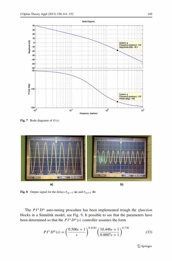
The output signal, used during the design phase, is shown in Fig. 6. It is possibleto note that the amplitude Ac = 1.261 V and the desired cross-over frequency ωu =1.9761 rad

s∼= ωcg are reached with the delay θa = 0.1296 s and the relay output |d| =

8 V. By substituting these values in (2) and (3) it is finally possible to determine themagnitude and the phase of the system, respectively −18.15 dB and −165.3◦.

As can be noted, see Fig. 7, the obtained values of the magnitude and phase ofG(s) at the cross-over frequency are very close to the real ones.

Once the module and the phase of experimental system are determined, the tuningphase of the PIλDμ controller starts.

To estimate the phase slope around ωcg , a value of θcg−δ equal to 0.0796 s isapplied in (8) obtaining θcg+δ = 0.1796 s. In Figs. 8(a) and 8(b) it possible to see thecorresponding frequencies: ωcg−δ = 2.575 rad

s ωcg+δ = 1.671 rads , respectively.

From (3) it is now possible to determine the phases: ϕ(jωcg−δ) = −2.937 rad andϕ(jωcg+δ) = −2.841 rad and then the phase slope ν = −0.1058 is obtained from (7).


Fig. 7 Bode diagrams of G(s)

Fig. 8 Output signal for the delays θcg−δ (a) and θcg=δ (b)

The PIλDμ auto-tuning procedure has been implemented trough the sfunctionblocks in a Simulink model, see Fig. 9. It possible to see that the parameters havebeen determined so that the PIλDμ(s) controller assumes the form

PIλDμ(s) =(

0.506s + 1

s

)0.4181(10.446s + 1

0.0007s + 1

)0.736

(33)


3.2 Experimental Control System

The Simulink model of the PIλDμ controller is shown in Fig. 10. The integro-differential equations of fractional order have been implemented according to thedefinition of Grunwald–Letnikov as in [27].

The “CaptureSettings” instrument is added in the ControlDesk project for the ac-quisition of the step responses while varying the open-loop gain K .

The step responses of the controlled system are shown in Fig. 11. We observethat the system exhibits robust performances to gain variations, keeping constant theovershoot of the step responses.

4 Concluding Remarks

An auto-tuning method for fractional order PIλDμ controller has been implementedon hardware in the loop board. The method allows a flexible and direct selection ofthe parameters of the controller through the knowledge of the magnitude and phaseof the plant at the frequencies of interest. Specifications on cross-over frequency, ωcg ,and phase margin, ϕm, can be easily fulfilled guaranteeing an iso-damping responseof the system versus gain variations. Experimental results illustrate the effectivenessof the proposed approach showing also robustness to the gain variation.

Fig. 9 PIλDμ auto-tuningprocedure in ControlDesk ondSPACE system

Fig. 10 RTI block diagram of the fractional experimental system for different gain values


Fig. 11 Step responses withdifferent gain values

Acknowledgements This work has been supported by the Italian Ministry of University and Re-search (MIUR) under PRIN projects “Non-integer order systems in modeling and control”, grant no.2009F4NZJP.

References

1. Podlubny, I.: Fractional order systems and PID controller. IEEE Trans. Autom. Control 44(1), 208–214 (1999)

2. Vinagre, B., Podlubny, I., Dorcak, L., Felin, V.: On fractional PID controllers: a frequency domainapproach. In: IFAC WorkShop on Digital Control, Past, Present, and Future of PID Control, Terrasa,Spain, pp. 53–58 (2000)

3. Vinagre, B.: Modelling and control of dynamic systems characterized by integro-differential equationsof fractional order, Ph.D. thesis, UNED, Madrid, Spain (2001)

4. Vinagre, B., Monje, C., Calderón, A.: Fractional order systems and fractional order control actions.In: 41st Conference on Decision and Control, Tutorial Workshop 2: Fractional Calculus Applicationsin Automatic Control and Robotics, Las Vegas (2002)

5. Chen, Y.: Ubiquitous fractional order controls. In: 2nd IFAC Symposium on Fractional Derivativesand Its Applications (IFAC FDA06), Porto, Portugal (2006)

6. Manabe, S.: A suggestion of fractional-order controller for flexible spacecraft attitude control. Non-linear Dyn. 29, 251–268 (2002)

7. Machado, T.: Analysis and design of fractional-order digital control systems. Syst. Anal. Model.Simul. 27, 107–122 (1997)

8. Oustaloup, A., Moreau, X., Nouillant, M.: The crone suspension. Control Eng. Pract. 4(8), 1101–1108(1996)

9. Caponetto, R., Fortuna, L., Porto, D.: Parameter tuning of a non-integer order PID controller. In: 15thInternational Symposium on Mathematical Theory of Networks and Systems, Notre Dame, Indiana(2002)

10. Caponetto, R., Fortuna, L., Porto, D.: A new tuning strategy for non integer order PID controller. In:First IFAC Workshop on Fractional Differentiation and Its Application, Bordeaux, France (2004)

11. Caponetto, R., Dongola, G. Fortuna, L., Gallo, A.: New results on the synthesis of FO-PID controllers.Commun. Nonlinear Sci. Numer. Simul. 15(4), 997–1007 (2010)

12. Caponetto, R., Dongola, G.: Field programmable analog array implementation of noninteger orderPIλdμ controller. Journal of Computational and Nonlinear Dynamics 3(2), 021302 (2008)

13. Leu, J.F., Tsay, S.Y., Hwang, C.: Design of optimal fractional-order PID controllers. J. Chin. Inst.Chem. Eng. 33(2), 193–202 (2002)

14. Barbosa, R., Tenreiro, J.A., Ferreira, I.M.: A fractional calculus perspective of PID tuning. In: ASMEDesign Engineering Technical Conferences and Computers and Information in Engineering Confer-ence, Chicago, USA (2003)


15. Barbosa, R., Tenreiro, J.A., Ferreira, I.M.: PID controller tuning using fractional calculus concepts.Fract. Calc. Appl. Anal. 7(2), 119–134 (2004)

16. Barbosa, R., Tenreiro, J.A., Ferreira, I.M.: Tuning of PID controllers based on Bode’s ideal transferfunction. Nonlinear Dyn. 38(1–4), 305–321 (2004)

17. Chen, Y., Moore, K., Vinagre, B., Podlubny, I.: Robust PID controller autotuning with a phase shaper.In: First IFAC Workshop on Fractional Differentiation and Its Applications, Bordeaux, France, pp.162–167 (2004)

18. Chen, Y.Q., Vinagre, B.M., Podlubny, I.: Continued fraction expansion approaches to discretizingfractional order derivatives, an expository review. Nonlinear Dyn. 38(1–4), 155–170 (2004)

19. Chen, Y.Q., Vinagre, B.M., Monje, C.: A proposition for the implementation of non-integer PI con-trollers. In: Thematic Action Systems with Non-integer Derivations, Bordeaux, France (2003)

20. Monje, C., Calderon, A., Vinagre, B.: PI vs. fractional DI control: first results. In: 5th PortugueseConference on Automatic Control, Aveiro, Portugal, pp. 359–364 (2002)

21. Valerio, D., Da Costa, J.: Tuning-rules for fractional PID controllers. In: Second IFAC Workshop onFractional Differentiation and Its Application, Porto, Portugal (2006)

22. Chen, Y., Dou, H., Vinagre, B.M., Monje, C.: Robust tuning method for fractional order PI controllers.In: Second IFAC Workshop on Fractional Differentiation and Its Application, Porto, Portugal (2006)

23. Monje, C., Vinagre, B.M., Feliu, V., Chen, Y.: On auto-tuning of fractional order PIλdμ controllers.In: Second IFAC Workshop on Fractional Differentiation and Its Application, Porto, Portugal, pp.19–21 (2006)

24. Monje, C., Vinagre, B.M., Feliu, V., Chen, Y.: Tuning and auto-tuning of fractional order controllersfor industry applications. Control Eng. Pract. 16, 798–812 (2007)

25. Santamaria, G.E., Tejado, I., Vinagre, B.M., Monje, A.: Fully automated and tuning and implementa-tion of fractional PID controllers. In: 7th International Conference on Multibody Systems, NonlinearDynamics and Control, vol. 4, San Diego, California, USA, pp. 1275–1283 (2009)

26. dSPACE: ControlDesk Experiment Guide, for release 3.4, User’s guide, May, 200227. Oldham, K.B., Spanier, J.: The Fractional Calculus: Theory and Applications of Differentiation and

Integration to Arbitrary Order. Dover Books on Mathematics, vol. 234. Academic Press, New York(2006)

art%3a10.1007%2fs10957-012-0235-y

Documents