MNRAS 000, 1–16 (2017) Preprint 21 November 2017 Compiled using MNRAS LATEX style file v3.0

A dearth of small particles in the transiting materialaround the white dwarf WD 1145+017

S. Xu1?, S. Rappaport2, R. van Lieshout3, A. Vanderburg4, B. Gary5,

N. Hallakoun6,1, V. D. Ivanov1,7, M. C. Wyatt3, J. DeVore8, D. Bayliss9, J. Bento10,A. Bieryla4, A. Camero11 J. M. Cann12, B. Croll13, K. A. Collins4, P. A. Dalba13,

J. Debes14, D. Doyle15, P. Dufour16, J. Ely17, N. Espinoza18, M. D. Joner19 ,

M. Jura20, T. Kaye21, J. L. McClain15,22, P. Muirhead13, E. Palle23,24, P. A. Panka12,

J. Provencal25, S. Randall1, J. E. Rodriguez4, J. Scarborough15, R. Sefako26,

A. Shporer27, W. Strickland15, G. Zhou4, B. Zuckerman20

Affiliations are listed at the end of the paper.

Accepted 2017 November 14. Received 2017 November 14; in original form 2017 August 09

ABSTRACTWhite dwarf WD 1145+017 is orbited by several clouds of dust, possibly emanatingfrom actively disintegrating bodies. These dust clouds reveal themselves through deep,broad, and evolving transits in the star’s light curve. Here, we report two epochs ofmulti-wavelength photometric observations of WD 1145+017, including several filtersin the optical, Ks and 4.5 µm bands in 2016 and 2017. The observed transit depthsare different at these wavelengths. However, after correcting for excess dust emissionat Ks and 4.5 µm, we find the transit depths for the white dwarf itself are the same atall wavelengths, at least to within the observational uncertainties of ∼5%-10%. Fromthis surprising result, and under the assumption of low optical depth dust clouds,we conclude that there is a deficit of small particles (with radii s . 1.5 µm) in thetransiting material. We propose a model wherein only large particles can survive thehigh equilibrium temperature environment corresponding to 4.5 hr orbital periodsaround WD 1145+017, while small particles sublimate rapidly. In addition, we evaluatedust models that are permitted by our measurements of infrared emission.

Key words: eclipses – minor planets, asteroids: general – stars: individual:WD 1145+017 – white dwarfs.

1 INTRODUCTION

Recent studies show that relic planetary systems or theirdebris are widespread around white dwarfs. About 25-50%of white dwarfs show “pollution” from elements heavier thanhelium in their atmospheres (Zuckerman et al. 2003, 2010;Koester et al. 2014). The most heavily polluted white dwarfsoften display excess infrared emission from a dust disc withinthe white dwarf’s tidal radius (e.g. von Hippel et al. 2007;Farihi et al. 2009). About 20% of these dusty white dwarfsalso display double-peaked calcium infrared triplet emissionlines from orbiting gas debris which spatially coincides withthe dust disc (e.g. Gansicke et al. 2006; Brinkworth et al.

? E-mail: sxu@gemini.edu

2009; Melis et al. 2010). A widely accepted model is that thewhite dwarfs are accreting debris of disrupted minor planetsthat survived the post-main-sequence evolution of the white-dwarf progenitor. These minor planets would have been per-turbed into the white dwarf’s tidal radius and subsequentlydisrupted (Debes & Sigurdsson 2002; Jura 2003). Therefore,high-resolution spectroscopic observations of the heavily pol-luted white dwarfs can uniquely reveal the bulk chemicalcompositions of these extrasolar minor planets (Zuckermanet al. 2007; Jura & Young 2014).

No evidence, however, for such a disintegrating mi-nor planet has ever been directly identified until rela-tively recently. WD 1145+017 happened to be observedby the K2 mission (in Campaign 1), and it was observedto display transits with multiple periods ranging from 4.5-

c© 2017 The Authors

arX

iv:1

711.

0696

0v1

[as

tro-

ph.E

P] 1

9 N

ov 2

017

2 Xu, Rappaport, & van Lieshout et al.

4.9 hours (Vanderburg et al. 2015). Followup observationscame quickly (e.g. Gansicke et al. 2016; Rappaport et al.2016; Gary et al. 2017; Croll et al. 2017) and found thatthe transit durations range from ∼ 3 min to as long as anhour—much longer than expected for a solid body (Van-derburg et al. 2015). The transits are inferred to be causedby the passage of dust clouds rather than solid bodies. Pre-sumably each periodicity represents the orbit of a differentunderlying body that supplies the dusty effluents. In turn,these bodies are currently hypothesised to be fragments fromthe tidal disruption of an asteroidal parent body. At theseorbital periods all the orbiting objects lie close to the whitedwarf’s tidal radius. The transit profiles are variable, asym-metric, and display depths up to 60% (e.g. Gansicke et al.2016; Rappaport et al. 2016; Gary et al. 2017; Croll et al.2017); they are morphologically similar to transits of disin-tegrating planets around main-sequence stars (e.g. Rappa-port et al. 2012). On a timescale of a few weeks, there canbe significant evolution of the transit shape and depth (e.g.Gansicke et al. 2016; Gary et al. 2017; Croll et al. 2017). Theorigin, creation mechanism, and lifetimes of these orbitingbodies are currently uncertain at best, with inferred massesin the range of 1017 −1024 g (Vanderburg et al. 2015; Rappa-port et al. 2016). Additional dynamical simulations supportthe statement that the orbiting objects should be no moremassive than Ceres (Gurri et al. 2017). In order to producethe observed transit features, the disintegrating objects arelikely to be in circular orbits and also differentiated (Veraset al. 2017).

When observed with the Keck Telescope, WD 1145+017was found to display photospheric absorption lines from 11elements heavier then helium, making it one of the mostheavily polluted white dwarfs known (Xu et al. 2016). In ad-dition, a uniquely rich set of circumstellar absorption linesfrom 7 elements was detected. These lines tend to have largevelocity dispersions (∼ 300 km s−1), and may well be associ-ated with gas orbiting near the white dwarf (i.e., at distancesof ∼5-15 white dwarf radii; Redfield et al. 2017; Vander-burg & Rappaport 2018). The circumstellar line profiles havechanged significantly since their original discovery (Redfieldet al. 2017). In addition, WD 1145+017 displays infraredexcess from orbiting dust particles (Vanderburg et al. 2015).

There have been several attempts with multi-wavelength observations to constrain the properties of thetransiting material. If the transits are caused by opticallythin dust passing in front of the star, the transit depthsshould be wavelength dependent due to the wavelength de-pendence behaviours of Mie scattering cross sections. Fromsimultaneous V- and R-bands observations, Croll et al.(2017) concluded that the particle radii must be larger than0.15 µm or smaller than 0.06 µm. Alonso et al. (2016) re-ported observations from 4800 to 9200 A and found no dif-ference in the transit depth across that wavelength range.They concluded that particle sizes less than 0.5 µm can beexcluded for the common minerals. Zhou et al. (2016) ex-tended the observations to J band and still found no wave-length dependence of the transits. They placed a 2 sigmalower limit on the particle size of 0.8 µm. The first detectionof a wavelength-dependent transit was recently reported inHallakoun et al. (2017), which features “bluing” – transitsare shallower in the u’ band than those in the r’ band, incontrast to the usual expectation in a dusty environment.

After exploring different scenarios, they concluded that themost likely explanation is the reduced absorption of circum-stellar lines during transits.

In this work we extend the photometric observations to4.5 µm. This paper is organised as follows. In Sect. 2 wepresent the details of our observations and the data analysismethods. In Sect. 3 we derive transit depth ratios and findthat they are consistent at all the observed wavelengths. Weinterpret this as a result of the prevalence of large grains inSect. 4. We explore a model that would explain the dearthof small grains in Sect. 5. The connection between the tran-siting material and the infrared excess is discussed in Sect. 6and the conclusion is given in Sect. 7.

2 OBSERVATIONS AND DATA REDUCTION

We have carried out two epochs of multi-wavelength photo-metric observations that cover optical to 4.5 µm during both2016 March 28-29 and 2017 April 4-5. The observing logs arelisted in Table 1 and the light curves are shown in Figs. 1 and2. We describe the observations and data reduction methodsin the following section.

2.1 WET & Perkins: Optical

For the optical observation in 2016, we used the 0.6m Paul& Jane Meyer Observatory Telescope in the Whole EarthTelescope (WET) network with the BG 40 filter. Data re-duction was performed following the procedures developedfor the WET observations (Provencal et al. 2012). Therewere passing (terrestrial) clouds, which caused some gapsand increased scatter in certain portion of the light curve,as shown in Fig. 1.

During the 2017 observing run, we arranged observa-tions with several optical telescopes. The details of theseobservations are described in Appendix A. Here, we focuson data taken on the 1.8m Perkins telescope at the LowellObservatory using the Perkins Re-Imaging System (PRISM,Janes et al. 2004), which has the best data quality. The ob-servation was designed following previous WD 1145+017 ob-servations (Croll et al. 2017). The observing conditions weremoderately good. Seeing was around 3.′′0 and there were thincirrus clouds at the beginning of the observation, which de-veloped substantially throughout the night. Data reductionwas performed following a custom pipeline (Dalba & Muir-head 2016; Dalba et al. 2017).

2.2 VLT/HAWKI: Ks

On 2016 March 28-29, WD 1145+017 was monitored in Ks

band with the HAWK-I (High Acuity Wide field K-band Im-ager; Pirard et al. 2004) at the Very Large Telescope (VLT).The camera is equipped with four HAWAII 2RG 2048×2048detectors, with a plate scale of ∼0.′′106 pixel−1. We used theFast Jitter mode that allows one to window down the detec-tors, greatly reducing the readout overheads. Following sim-ilar procedures outlined in Caceres et al. (2011), we appliedwindows of 128×256 pixels per detector stripe. We recordeda sequence of blocks, each consisting of 60 exposures with 15s integration time. Throughout the observations, we kept thenearby star ULAS J114829.42+012707.6 (Ks=16.678±0.042)

MNRAS 000, 1–16 (2017)

A dearth of small particles around WD 1145+017 3

Table 1. Observing logs

Instrument Central Wavelength Observing Time (UT) Exposure Time (s)

2016Meyer 0.48 µm Mar 28, 21:00 - Mar 29, 04:37a 60

VLT/HAWK-I 2.1 µm (Ks) Mar 29, 03:43 - 06:28 15

Spitzer/IRAC 4.5 µm Mar 28, 22:18 - Mar 29, 06:04 30

2017Perkins/R 0.65 µm Apr 5, 03:12 - 09:50 45

VLT/HAWKI 2.1 µm (Ks) Apr 5, 00:33 - 07:19 15, 30b

Spitzer/IRAC 4.5 µm Apr 4, 22:42 - Apr 5, 08:33 30

Note.aThere are some gaps in the light curve due to passing clouds.

bThe first set of observations (∼ 75 min) was executed in 15 s exposure time.

0.5

1.0

1.5

A1 A1

WET:Optical

0.5

1.0

1.5

VLT:Ks

0.05 0.00 0.05 0.10 0.15 0.20 0.25MJD(-57476)

0.5

1.0

1.5

Spitzer:4.5 m

0 100 200 300 400 500Minutes

Nor

mal

ised

Flu

x

Figure 1. The light curves from all the observations on March 28-29, 2016. There was one main transit feature during a full period of270 min and we denote it as A1. For the Ks and 4.5 µm band observations, the grey dots represent individual measurements. The yellowdots are smoothed with every 3 data points and the red dots are smoothed every 5 data points.

on the same detector as the science target to provide a fluxreference. The weather conditions were moderate and therewere thin clouds passing by during the observations. TheDIMM seeing was about 0.′′55 in the optical.

Individual images were dark-subtracted and flat-fieldcorrected with sky flats taken immediately after the obser-vation. Aperture photometry was performed with aperture

radii of 5, 7, and 10 pixels. The sky background was esti-mated from an annulus of between 10 and 20 pixels. Wefound that the light curve from the 7 pixel (0.′′75) radiusaperture has the best quality and use this light curve forthe rest of our analysis. Both the target light curve and thereference star light curve were normalised by dividing by aconstant, as shown in Fig. 3.

MNRAS 000, 1–16 (2017)

4 Xu, Rappaport, & van Lieshout et al.

0.5

1.0

1.5

B1 B2 B3

Perkins:Optical

0.5

1.0

1.5

VLT:Ks

0.05 0.00 0.05 0.10 0.15 0.20 0.25 0.30 0.35MJD(-57848)

0.5

1.0

1.5

Spitzer:4.5 m

0 100 200 300 400 500 600Minutes

Nor

mal

ised

Flu

x

Figure 2. The light curves from all the observations on April 4-5, 2017. There are three main transit features in a full period of 270

min, denoted as B1, B2, and B3. All the notations are the same as those in Fig. 1.

We repeated the observations with HAWK-I on April 4-5, 2017 with a similar set-up. The observing conditions werebetter: clear sky with optical seeing at the beginning of 1.′′0,which decreased to 0.′′5 toward the end of the observation.We started the observations with a block of 60 exposureswith 15 s integration each. We repeated this block five timesbefore noticing that the target was not visible in the guider.Out of concern that the target had drifted out of the smallfield of view, we stopped the sequence, reacquired the tar-get, and increased the exposure time to 30 s. After that, weobserved in blocks consisting of 30 exposures with 30-s inte-gration times until the end of the observation.

Data reduction was performed following the samemethod as for the 2016 dataset. We adopted an apertureradius of 8 pixels (0.′′85), and a sky annulus between 10 and20 pixels for aperture photometry. In retrospect, our targetdid not disappear around 57848.08 (MJD); in fact, there wasa deep transit, which made the target difficult to see in indi-vidual images. Because the data quality was better with 30-sexposure time, we focus on these for the following analysis.

2.3 Spitzer/IRAC: 4.5 µm

We were awarded time with the Infrared Array Camera(IRAC; Fazio et al. 2004) on the Spitzer Space Telescope

under a DDT program to observe WD 1145+017 simulta-neously with the VLT on March 28-29, 2016. The observa-tion was designed following “Advice for designing high pre-cision photometry observations”1. The science observationsconsisted of 900 exposures of 30 s each in the 4.5 µm filterin stare mode. The readout mode was full array. The targetwas put in the well-characterised pixel (“sweet spot”). Beforethe science observation, we arranged a 30-minute exposureto eliminate the initial drift of the instrument (Grillmairet al. 2012). We also included a 10-minute post-observationwith the same setup as the pre-observation.

For the data reduction, we started with the CBCD (Cor-rected Basic Calibrated Data) files, which are flux-calibratedand artefact-corrected files from the pipeline (IRAC Instru-ment Handbook). We excluded a few frames when therewas a cosmic ray close to the target. The pre-observationand post-observation frames were median combined andsmoothed to create a localised dark frame, which was thensubtracted from all CBCD files to remove any residual pat-terns. To produce the light curve, we used codes that arepublicly available for IRAC high precision photometry2. TheIDL program box centroider.pro was used to locate the

1 http://irachpp.spitzer.caltech.edu/page/Obs%20Planning2 http://irachpp.spitzer.caltech.edu/page/contrib

MNRAS 000, 1–16 (2017)

A dearth of small particles around WD 1145+017 5

0.16 0.18 0.20 0.22 0.24 0.26 0.28MJD(-57476)

0.0

0.5

1.0

1.5

2.0

2.5

Nor

mal

ised

Flu

x

ReferenceTarget

0 25 50 75 100 125 150 175Minutes

0.05 0.10 0.15 0.20 0.25 0.30MJD(-57848)

0.0

0.5

1.0

1.5

2.0

2.5

Nor

mal

ised

Flu

x

ReferenceTarget

0 50 100 150 200 250 300 350 400Minutes

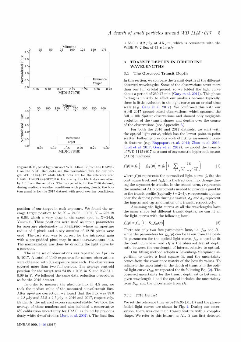
Figure 3. Ks band light curve of WD 1145+017 from the HAWK-

I on the VLT. Red dots are the normalised flux for our tar-get WD 1145+017 while black dots are for the reference star

ULAS J114829.42+012707.6. For clarity, the black dots are offset

by 1.0 from the red dots. The top panel is for the 2016 dataset,during mediocre weather conditions with passing clouds; the bot-

tom panel is for the 2017 dataset with good weather conditions.

position of our target in each exposure. We found the av-erage target position to be X = 24.08 ± 0.07, Y = 232.18± 0.08, which is very close to the sweet spot at X=24.0,Y=232.0. These positions were used as input parametersfor aperture photometry in aper.pro, where an apertureradius of 2 pixels and a sky annulus of 12-20 pixels wereused. The last step was to correct for the intrapixel gainwith a pre-gridded pixel map in iracpc pmap corr.pro.The normalization was done by dividing the light curve bya constant.

The same set of observations was repeated on April 4-5, 2017. A total of 1140 exposures for science observationswere obtained with 30 s exposure time each. The observationcovered more than two full periods. The average centroidposition for the target was 24.08 ± 0.08 in X and 232.31 ±0.09 in Y. We followed the same data reduction proceduresas for the 2016 dataset.

In order to measure the absolute flux in 4.5 µm, wetook the median value of the measured out-of-transit flux.After aperture correction, we found that the flux was 55.0± 2.3 µJy and 55.5 ± 2.5 µJy in 2016 and 2017, respectively.Evidently, the infrared excess remained stable. We took theaverage of these numbers and also included a conservative5% calibration uncertainty for IRAC, as found by previousdusty white dwarf studies (Jura et al. 2007b). The final flux

is 55.0 ± 3.2 µJy at 4.5 µm, which is consistent with theWISE W-2 flux of 43 ± 14 µJy.

3 TRANSIT DEPTHS IN DIFFERENTWAVELENGTHS

3.1 The Observed Transit Depth

In this section, we compare the transit depths at the differentobserved wavelengths. Some of the observations cover morethan one full orbital period, so we folded the light curveabout a period of 269.47 min (Gary et al. 2017). This phasefolding is unlikely to affect our analysis because typically,there is little evolution in the light curve on an orbital timescale (e.g. Gary et al. 2017). We confirmed this with ourApril 2017 ground-based observations, which spanned thefull ∼ 10h Spitzer observations and showed only negligibleevolution of the transit shapes and depths over the courseof the observations (see Appendix A).

For both the 2016 and 2017 datasets, we start withthe optical light curve, which has the lowest point-to-pointscatter. Following previous work of fitting asymmetric tran-sit features (e.g. Rappaport et al. 2014; Zhou et al. 2016;Croll et al. 2017; Gary et al. 2017), we model the transitsof WD 1145+017 as a sum of asymmetric hyperbolic secant(AHS) functions:

f (p) = f0

[1 − fdip(p)

]≡ f0

1 −∑i

2 fi

ep−piφi1 + e−

p−piφi2

(1)

where f (p) represents the normalised light curve, f0 fits thecontinuum level, and fdip(p) is the fractional flux change dur-ing the asymmetric transits. In the second term, i representsthe number of AHS components needed to provide a good fitto the transit profile (typically i = 2−4), pi represents a phasenear the deepest point during a transit, φi1 and φi2 representthe ingress and egress duration of a transit, respectively.

Assuming the light curves at all the wavelengths havethe same shape but different transit depths, we can fit allthe light curves with the following form,

fλ(p) = fλ,0[1 − Dλ fdip(p)

](2)

There are only two free parameters here, i.e. fλ,0 and Dλ,while the parameters for fdip(p) can be taken from the best-fit parameters for the optical light curve. fλ,0 is used to fitthe continuum level and Dλ is the observed transit depthratio between the wavelength of interest relative to optical.

Our fitting method adopts a Levenberg-Marquardt al-gorithm to derive a least square fit, and the uncertaintycomes from the covariance matrix of the best fit values. Toestimate the uncertainty in the depth of transits in the opti-cal light curve Dopt, we repeated the fit following Eq. (2). Theobserved uncertainty for the transit depth ratios between agiven wavelength λ and the optical includes the uncertaintyfrom Dopt and the uncertainty from Dλ.

3.1.1 2016 Dataset

We set the reference time as 57475.95 (MJD) and the phase-folded light curves are shown in Fig. 4. During our obser-vation, there was one main transit feature with a complexshape. We refer to this feature as A1. It was first detected

MNRAS 000, 1–16 (2017)

6 Xu, Rappaport, & van Lieshout et al.

on January 21, 2016 (denoted as ‘G6121’ in Gary et al. 2017and ‘A1’ in Hallakoun et al. 2017). This feature was wellcovered in the optical, Ks band, 4.5 µm.

For the WET light curve, we used three AHS compo-nents for A1 following Eq. (1) and the best-fit parametersare listed in Table 2. We fitted all the light curves withthe same functional form but different transit depth D withEq. (2), with the results listed in Table 3. The observedtransit depths are different at all three wavelengths.

3.1.2 2017 Dataset

We set the reference time as 57848.13 (MJD) and the phase-folded light curves are shown in Fig. 5. There were threemain transit features during a full orbital period, denotedas B1, B2, and B3 (see Appendix A for details). The B1Dip was shallow and not detected in the Ks band nor theSpitzer band, due to their relatively low signal-to-noise ra-tios compared to the optical light curve. Here, we focus ontransits B2 and B3, which are better suited for studying thewavelength-dependence of the transits. We believe B2 wasdue to the same orbiting body that produced A1 in 2016and B3 could be related to some other features observed inthe previous season as well (Rappaport et al. 2017).

We followed the same analysis procedures outlined inSect. 3.1. We started with the Perkins light curve and usedthe functional form for Fdip(p) to fit the light curves at allthe wavelengths. The results are listed in Tables 2 and 3.The values for B2 and B3 are comparable, while the over-all uncertainties for B3 are smaller because the transit wasdeeper and lasted longer.

3.2 Transit Depth Correction for Dust Emission

In both datasets, we find that the transit depths of the ob-served flux are different at all the wavelengths. It is deepestin the optical and shallower at longer wavelengths. Thereis no change in the transit depth ratios between these twoepochs.

Because WD 1145+017 has an infrared excess startingfrom the Ks band (Vanderburg et al. 2015), this will neces-sarily dilute the transit signal. To derive the transit depthratio corrected for the dust emission, we need to use the in-trinsic white dwarf flux rather than the measured flux. Asa result, the corrected transit depth ratio can be calculatedas:

Dcorr =Fobs

F?

× D (3)

where Fobs and F? represents the measured out-of-transitflux and the expected flux from the white dwarf, respec-tively. We know that Fobs is constant during the two epochsof our observations. Based on the colour of WD 1145+017,we find that F? has little extinction from either circumstel-lar or interstellar material and therefore F? can be derivedfrom white dwarf model calculations. We take the correctionfactor Fobs/F? to be a constant.

We calculated white dwarf model spectra with param-eters listed in Table 4 and derived the fact that the whitedwarf flux is 53.5 µJy at Ks band and 13.0 µJy at 4.5 µm.Varying the temperature by 500 K and log g by 0.2 dex, wefound the white dwarf flux could change by at most 2% and

we adopted that as the uncertainty of the intrinsic whitedwarf flux. The measured total flux is 69.4 ± 5.2 µJy in Ks

band from the UKIDSS and 55.0 ± 3.2 µJy at 4.5 µm, asderived in Sect. 2.3. Therefore, the correction factors are(

Fobs

F?

)Ks

= 1.30 ± 0.10

(Fobs

F?

)4.5µm

= 4.23 ± 0.26.

Following Equ. (3), the corrected average transit depth ra-tios are: (

DKs

Dopt

)corr

= 0.96 ± 0.08

(D4.5µm

Dopt

)corr

= 1.13 ± 0.14

The corrected transit depths in Ks band and 4.5 µm areunexpectedly and even surprisingly consistent with the tran-sit depth in the optical, at least to within the uncertainties.This result tends to indicate that the extinction cross sec-tion is independent of wavelength for the observations fromoptical to 4.5 µm.

The main source of uncertainty for this analysis comesfrom the correction factor Fobs/F? in Eq. (3), which is mostlyfrom the uncertainty of the absolute flux measurements.Currently, it is 7.5% in Ks and 5.8% at 4.5 µm. Future obser-vations in the infrared will improve the flux measurement inKs band. However, IRAC observations will always be limitedby its absolute flux calibration, which is ∼ 5%.

In the following section, we explore possible physi-cal reasons for the wavelength-independence of the transitdepth.

4 CONSTRAINTS ON THE PARTICLE SIZE

The lack of a wavelength dependence of the transit depthscould be expected if the dust clouds are optically thick. How-ever, in order to explain both the transit depth and transitduration (e.g. the ∼20% deep and ∼90 min long transit re-ported in Alonso et al. 2016), an opaque cloud needs tobe both flat and also almost perfectly aligned with the or-bital direction. We therefore consider opaque clouds to bean unlikely explanation for the transiting material aroundWD 1145+017.

An alternative explanation for the colour-independenttransit depths is that large grains (i.e., & 1−2 µm) dominatethe extinction cross-section of the clouds and their cross-sections are nearly independent of wavelength out to 4.5 µm.

We explore the wavelength dependence of the extinctionefficiency (the ratio of the extinction cross section σext(X)to the geometric cross section), Qext ≡ σext(X)/πs2, where sis the particle radius, λ is the observing wavelength, andX ≡ 2πs/λ, the scaled particle size3. We adopted the Miealgorithm presented in Bohren & Huffman (1983) and the

3 We note that this simple functional form for Qext can only beused when the imaginary part of the complex index of refraction

is essentially independent of wavelength.

MNRAS 000, 1–16 (2017)

A dearth of small particles around WD 1145+017 7

0.6

0.8

1.0

1.2A1

WET:Optical

0.6

0.8

1.0

1.2

VLT:Ks

0.0 0.2 0.4 0.6 0.8 1.0Phase

0.6

0.8

1.0

1.2

Spitzer:4.5 m

0 50 100 150 200 250Minutes

Nor

mal

ised

Flu

x

Figure 4. Phase-folded transit light curve in the optical, Ks band, and 4.5 µm, respectively on March 28-29, 2016. The black line

represents the best-fit models with parameters listed in Tables 2 and 3.

Table 2. Best-fit parameters for the AHS components of different dip features in the optical band

Dip f0 i fi pi φi1 φi2

A1 1.003 ± 0.003 3 0.105 ± 0.012 0.231 ± 0.001 0.048 ± 0.011 0.002 ± 0.001

0.214 ± 0.025 0.306 ± 0.002 0.028 ± 0.007 0.003 ± 0.001

0.151 ± 0.023 0.375 ± 0.001 0.002 ± 0.001 0.073 ± 0.010

B1 1.001 ± 0.002 1 0.027 ± 0.006 0.147 ± 0.003 0.003 ± 0.002 0.042 ± 0.013

B2 0.979 ± 0.008 1 0.284 ± 0.026 0.456 ± 0.003 0.015 ± 0.004 0.008 ± 0.002

B3 0.979 ± 0.008 2 0.166 ± 0.022 0.622 ± 0.002 0.130 ± 0.017 0.004 ± 0.0020.276 ± 0.035 0.729 ± 0.009 0.027 ± 0.006 0.064 ± 0.010

Note.The parameters are defined in Eq. (1). We considered phase 0-0.3 for B1, 0.3-0.55 for B2, and 0.55-1.0 for B3. For different dips, f0 is

slightly different because of imperfect continuum normalisation.

results for a range of generic materials are shown in Fig. 6.Similar to results from previous studies (e.g. Croll et al.2014), we found that for very small values of X(. 0.1), Qext ∝

λ−1 is valid, while for large X & 2, Qext → 2, i.e., independentof λ. For intermediate values of X, Qext ∝ λ

−4.

Since we find a colourless transit depth between λ '

0.5 µm to 4.5 µm, we can reasonably infer that X & 2 evenat the longest wavelength of our observations. Specifically,we find that

X =2πsλ

& 2 (4)

Therefore, we tentatively conclude that our non-detection of

MNRAS 000, 1–16 (2017)

8 Xu, Rappaport, & van Lieshout et al.

Table 3. Transit depth ratios at the observed wavelengths

Dopt DKs DKs /Dopt D4.5µm D4.5µm/Dopt

A1 1.000 ± 0.021 0.664 ± 0.034 0.664 ± 0.037 0.256 ± 0.032 0.256 ± 0.032B2 1.000 ± 0.056 0.768 ± 0.057 0.768 ± 0.071 0.309 ± 0.073 0.309 ± 0.075

B3 1.005 ± 0.013 0.796 ± 0.018 0.792 ± 0.021 0.240 ± 0.026 0.239 ± 0.026

Average 0.741 ± 0.028 0.268 ± 0.029

Note.D is the best-fit parameter defined in Eq. (2). Dopt is not exactly unity because it depends on the range chosen to calculate the

out-of-transit flux, which is different for the B2 and B3 dips. The uncertainty in Dopt illustrates a minimum uncertainty even when

fitting the same data in different ways (with Eq. (1) and Eq. (2)).

0.4

0.6

0.8

1.0

1.2B1 B2 B3

Perkins:Optical

0.4

0.6

0.8

1.0

1.2

VLT:Ks

0.0 0.2 0.4 0.6 0.8 1.0Phase

0.4

0.6

0.8

1.0

1.2

Spitzer:4.5 m

0 50 100 150 200 250Minutes

Nor

mal

ised

Flu

x

Figure 5. Similar to Fig. 4 except for the 2017 dataset.

wavelength-dependent transit depths from optical to 4.5 µmimplies that the transiting material around WD 1145+017must consist of grains whose sizes are largely & 1.5 µm.

We can also compare the transit depth ratios at differentwavelengths with the corresponding Mie extinction cross sec-tions. We consider two generic grain materials (with n = 1.6and k = 0.1, 0.01), and two particle size distributions.

Hansen Distribution: For a range of characteristic par-ticle sizes of s = 0.2, 0.5, 1, 2, 5, 10 µm, the specific form of the

distribution is (Hansen & Travis 1974):

n(s) = Cs(1−3b)/be−s/sb

where C is a normalization constant, s is the particle radius,and b is the dimensionless variance of the distribution. Fol-lowing Zhou et al. (2016), we choose a value for b of 0.1,which provides a distribution that ranges from a factor ofroughly

√0.1 below s to a factor of

√10 above s. The nor-

malised distribution is then

n(s) =1

Γ(10)(0.1s)10 s7e−10s/s

MNRAS 000, 1–16 (2017)

A dearth of small particles around WD 1145+017 9

Table 4. WD 1145+017 system parameters

Parameter Symbol Value Reference

WD

Effective Temperature T? 15,900 K Vanderburg et al. (2015)Surface Gravity log g 8.0 Vanderburg et al. (2015)

Distance d 174 pc Vanderburg et al. (2015)

Mass M? 0.6 M Dufour et al. (2017)Radius R? 0.013 R Dufour et al. (2017)

Transiting MaterialOrbital Period P 269.47 min Gary et al. (2017)

Orbital Distance r 1.16 R Kepler’s third law

10!3 10!2 10!1 100 101 102 10310!6

10!5

10!4

10!3

10!2

10!1

100

101

X = 2:s=6

Qex

t

k = 1k = 0:1k = 0:01k = 0:001

Figure 6. Extinction efficiency as a function of scaled particlesize X for a range of grains with the real part of the index of

refraction n being fixed at 1.6 and the imaginary part k between0 and 1. For grains that satisfy X & 2, Qext is independent of

wavelength and remains a constant.

Cut-on Power-Law Size Distribution: we also consider aclassical power law distribution from a collisional cascade:

n(s) = Cs−3.5 (5)

where the minimum grain size smin is fixed. This distributionis probably a more realistic representation of the particlesize distribution as small grains may sublimate rapidly, asdiscussed in the next section. Note that in the cut-on power-law size distribution the effective particle size is larger thansmin.

As shown in Fig. 7, we find that for both size distri-butions, only grains larger than & 2 µm can explain theobserved transit depth ratios at the different wavelengths.

This minimum inferred grain size, for either choice ofsize distribution, is broadly consistent with the grain sizederived from modeling the 10 µm silicate emission featurearound other dusty white dwarfs (Reach et al. 2009; Juraet al. 2009). On the other hand, small dust (s . 1 µm) isprevalent in the interstellar medium (e.g. Mathis et al. 1977),while in the solar system the tails of comets and streamscoming off the active asteroids can be a mixture of smalland large grains (with s from sub-µm to cm), depending onthe dust production mechanism (e.g. Jewitt 2012).

5 A POSSIBLE MODEL: GRAINSUBLIMATION

In this section we explore a physical explanation for thedearth of small grains in the transiting dust clouds. In sum-mary, the explanation is that small grains have higher equi-librium temperatures than large grains, with the result thatthey are quickly destroyed by sublimation (see also von Hip-pel et al. 2007). The process of sublimation has an extremelysteep dependence on temperature, so a modest increase indust temperature can result in drastically shorter sublima-tion timescales. To assess this scenario, we first computethe equilibrium temperature of dust grains in the transit-ing clouds (Sect. 5.1), then evaluate whether sublimationoccurs in the potentially gas-rich circumstellar environmentof WD 1145+017 (Sect. 5.2), and finally calculate dust sub-limation timescales as a function of grain size (Sect. 5.3).Throughout this analysis we use the parameter values forthe WD 1145+017 system listed in Table 4.

5.1 Dust Temperatures

The temperature Td(s, r) of a dust grain with radius s atdistance r from the white dwarf can be calculated by solvingthe power balance between the incoming stellar radiationand the outgoing thermal radiation:

R2?

4r2

∫Qabs(s, λ)Bλ(λ,T?) dλ =

∫Qabs(s, λ)Bλ(λ,Td) dλ. (6)

The meanings for some symbols are listed in Table 4. Qabs

is the absorption efficiency of the dust grain, and Bλ is thePlanck function. The white dwarf spectrum is approximatedby blackbody radiation. This calculation ignores the latentheat of sublimation, which we find to be negligible (Rappa-port et al. 2014).

The grain temperature depends critically on the absorp-tion efficiency Qabs, which is generally a complicated functionof grain size s, wavelength λ, and the optical constants ofthe dust material, i.e., its complex refractive index n + ik. Incertain cases, however, simple prescriptions for Qabs can bederived, which allow the power balance Eq. (6) to be solvedanalytically (e.g. Backman & Paresce 1993; von Hippel et al.2007).

For grains that are very large compared to the radi-ation wavelength, the absorption efficiency asymptoticallyapproaches a constant value of Qabs ≈ 1. In this limit, solv-

MNRAS 000, 1–16 (2017)

10 Xu, Rappaport, & van Lieshout et al.

‘Cut-on’ Power-Law Size Distribution

Figure 7. Mie extinction cross sections at wavelength λ divided by the corresponding cross section at 0.6 µm (optical) for a generic grainmaterial, where n is set to be 1.6, and k = 0.1 (solid curves) and 0.01 (dashed curves). Two size distributions are shown. Left: Hansen

distribution, where the labels represent the characteristic particle sizes. Right: a ‘cut-on’ power-law size distribution (see definition in

Eq. (5)), where the labels represent the minimum grain size smin. We also show the measured transit depth ratios in WD 1145+017 (blackdots) as measured in this work. Only characteristic particle sizes of & 2 µm are consistent with the data.

ing Eq. (6) gives the blackbody temperature

Tbb =

√R?

2rT? (7)

≈ 1.2 × 103 K(

T?

15,900 K

) (R?

0.013 R

)1/2( r1.16 R

)−1/2

.

For very small grains, which fall in the Rayleigh regime,Qabs ∝ λ

−1 is found, which yields (e.g., Appendix C of Rap-paport et al. 2014)

TRayl =

(R?

2r

)2/5

T? (8)

≈ 2.0 × 103 K(

T?

15,900 K

) (R?

0.013 R

)2/5( r1.16 R

)−2/5

.

For general cases, the grain temperature can be foundby solving Eq. (6) using Qabs from the Mie theory (Bohren& Huffman 1983). In Fig. 8 we plot grain temperatures as afunction of grain size. This shows the convergence towardsthe limiting temperatures for small and large grain sizes.Small grains can reach a much higher temperature of 2000 Kthan large grains of 1200 K. Interestingly, for dust orbitingWD 1145+017 in a 4.5 hr period, the values of the two lim-iting temperatures bracket the temperatures at which manyrefractory materials sublimate rapidly.

5.2 The Sublimation/Condensation Balance

Like all thermodynamic phase transitions, sublimation de-pends on the pressure and temperature of the matter in-volved, and the balance between sublimation and conden-sation can be evaluated using a phase diagram. For a giventemperature T , the pressure at which these two processes arein equilibrium is called the phase-equilibrium (or saturated)vapour pressure psat. Based on the Clausius–Clapeyron rela-tion, its temperature dependence is found to be

psat(T ) = exp(−A/T + B ), (9)

where A and B are material-dependent sublimation param-eters that can be determined experimentally. Dust grainswith temperature Td will sublimate when the ambient gaspressure pg is lower than psat(Td), while condensation hap-pens for pg > psat(Td).

To assess whether sublimation or condensation domi-nates, we make a rough estimate of the ambient gas pressure.Assuming the gas around the white dwarf forms a steady-state viscous accretion disc, where the viscosity is parame-terised by αν, the gas pressure in the disc is given approxi-mately by (Rafikov & Garmilla 2012)

pg =MΩ2

K

3πανcs(10)

≈ 0.2 dyn cm−2(

M1010 g s−1

) (P

4.5 hr

)−2(αν

0.01

)−1( cs

1 km s−1

)−1

.

Here, ΩK is the local Keplerian angular frequency and cs isthe sound speed. The mass accretion rate M can be esti-mated from pollution in the white dwarf’s atmosphere, as-suming a steady state accretion (Xu et al. 2016). In addition,cs ∼ 1 km s−1 is a reasonable estimate for the sound speed ofa metallic gas with a temperature of a few thousand K, sothe uncertainty in pg is dominated by the poor knowledgeof αν. Note that the temperature and vertical distribution ofthe gaseous disc can be substantially different from that ofthe dust (sect. 6 in Melis et al. 2010).

Fig. 9 shows a comparison of the phase-equilibriumvapour pressures of a set of possible refractory materials, ex-cluding graphite4(using values of A and B in Table 3 of vanLieshout et al. 2014) with the estimated ambient gas pres-sure associated with the presumed gaseous accretion disc.

4 Graphite is unlikely to be the dominant component of the dust

particles because carbon has not yet been detected in the atmo-

sphere of WD 1145+017 (Xu et al. 2016). In fact, almost all pol-luted white dwarfs are carbon-depleted (e.g. Jura 2006). Graphite

is excluded for all the following analyses.

MNRAS 000, 1–16 (2017)

A dearth of small particles around WD 1145+017 11

Td = TRayl

Td = Tbb

0:001 0:01 0:1 1 10 100 1000500

1000

1500

2000

2500

grain radius s [7m]

dust

tem

per

ature

Td

[K]

k = 1k = 0:1k = 0:01k = 0:001

Figure 8. Temperature as a function of grain size for dust grains

in orbit around WD 1145+017 at 4.5 hr. The solid coloured linesrepresent generic minerals with different values of k, the imagi-

nary part of the index of refraction. The real part is kept fixed

at n = 1.6. Also shown are the two limiting cases of Rayleigh-approximation and blackbody temperatures (dashed horizontal

lines). Small grains are heated to a higher temperature than large

grains.

Although there is great uncertainty in both psat (becausethe dust composition is not well constrained) and pg (be-cause αν is unknown), the figure reveals that sublimationis expected for dust with temperatures around TRayl (smallgrains), while material with temperatures around Tbb (largegrains) could be protected from sublimation by the gas disc.

5.3 A Minimum Grain Size Due to Sublimation

Because the Rayleigh-approximation temperature is higherthan the blackbody temperature (TRayl/Tbb ≈ 1.7), the dusttemperature must go up with decreasing grain size. Dustsublimation rates have an extremely steep dependence ontemperature, so this increase in temperature will be associ-ated with a dramatic decrease in dust survival time againstsublimation. In contrast, when the dust temperature is con-stant with grain size, the sublimation timescale will onlydecrease linearly with decreasing grain size.

To quantify the effect of sublimation on grain survivaltimes, we compute dust sublimation timescales, given by

tsubl = −ss

=sρd

J(Td). (11)

Here, s is the grain radius, s is its change rate, ρd is thedensity of the dust material, and J is the net sublimationmass-loss flux (units: [g cm−2 s−1]; positive for mass loss). Themass-loss flux J can be calculated from the kinetic theory ofgasses (e.g. Langmuir 1913):

J(T ) = αsubl

[psat(T ) − pg

] õmu

2πkBT. (12)

Here, αsubl is the evaporation coefficient, also known as the‘accommodation coefficient’ or ‘sticking efficiency’, whichparametrises kinetic inhibition of the sublimation process(which we assume to be independent of temperature), µ isthe molecular weight of the molecules that sublimate, mu isthe atomic mass unit, and kB is the Boltzmann constant.

Tbb

Tss

TRayl

max(T

d)

IronSiOFayaliteEnstatiteForsteriteQuartzCorundumSiC

,8 = 0:001

,8 = 0:01

,8 = 0:1

,8 = 1

500 1000 1500 2000 2500

10!5

100

105

temperature T [K]

pressure

[dyncm

!2]

Figure 9. Phase-equilibrium vapour pressure psat as function

of temperature for a set of possible dust species from Eq. (9)

(coloured lines), together with estimates of the ambient gas pres-sure pg for several different values of the viscosity parameter ανfrom Eq. (10) (horizontal black lines). Sublimation occurs when pg< psat, while condensation happens when pg > psat. Also indicatedare temperatures reached by particles orbiting WD 1145+017 in

several limiting cases (dashed vertical lines): Tbb, the blackbodytemperature valid for large dust grains; Tss, the temperature at the

substellar point of a tidally locked large body (based on eq. (5)

in Vanderburg et al. 2015); TRayl, the limiting temperature forsmall grains; and max(Td), the maximum dust temperature seen

in Fig. 8.

In Fig. 10, we show the sublimation timescale as afunction of grain size using dust temperatures computed inSect. 5.1. The calculation uses a set of sublimation parame-ters typical for a generic refractory material: A = 65,000 K,B = 35, ρd = 3 g cm−3, αsubl = 0.1, and µ = 100. These fallroughly in the middle of the range of values seen for the re-fractory materials shown in Fig. 9 (see van Lieshout et al.2014).

Fig. 10 demonstrates that small dust is destroyed al-most instantaneously, while large dust could survive againstsublimation for many years. This result is robust despite thelarge uncertainty in sublimation timescale introduced by theuncertainty in dust composition and hence sublimation pa-rameters (there are about 2 to 4 orders of magnitude spreadin sublimation timescale amongst the materials shown inFig. 9). We conclude that the large grain sizes inferred fromthe lack of wavelength dependence in the transit depths ofWD 1145+017 is likely the result of sublimation of smallergrains, because of their higher equilibrium temperatures andrapid sublimation. This conclusion holds when consideringboth gas-free and gas-rich environments. In the gas-free case,large grains have very long sublimation timescales, and theirlifetime is likely set by other destruction processes than sub-limation. In the gas-rich case, large grains are also protectedfrom sublimation by the gas disc (as discussed in Sect. 5.2).

Our method of estimating sublimation timescales as-sumes the temperature of the dust grain to remain constantas it decreases in size due to sublimation, which is incorrectas shown in Fig. 8. However, given the extreme tempera-

MNRAS 000, 1–16 (2017)

12 Xu, Rappaport, & van Lieshout et al.

1 s

1 hr

1 yr

0:001 0:01 0:1 1 10 100 100010!10

10!5

100

105

1010

grain radius s [7m]

sublim

atio

ntim

et s

ubl[d

ay]

k = 1k = 0:1k = 0:01k = 0:001

gas-freepg = 0:2 dyn cm!2

Figure 10. Sublimation timescale as function of grain size assum-

ing the dust temperatures from Fig. 8 and sublimation parameterscorresponding to a generic refractory material. Different coloured

lines correspond to different values of the imaginary part of the

complex refractive index k. The real part is kept fixed at n = 1.6.The solid curves are for dust grains in vacuum; the dashed curves

assume an ambient gas density of pg ≈ 0.2 dyn cm−2 (see Sect. 5.2).

The error bar is a rough indication of the uncertainty in sublima-tion time found by considering different possible dust materials

(specifically, those listed in Fig. 9.)

ture dependence of the sublimation process, the sublima-tion timescale will be dominated by the lowest dust temper-atures encountered. Hence, Eq. (11) using the initial dusttemperature provides a very good estimate of the sublima-tion timescale.

The exact value of the grain size s below which subli-mation destroys grains faster than they are replenished de-pends on a number of factors: the optical properties of thedust (most importantly the value of the imaginary part ofthe complex refractive index k); its sublimation parameters(i.e. A, B, αsubl, µ, and ρd); the timescale on which otherprocesses (like collisions) destroy dust grains when the sub-limation timescale is long; and the size-dependent input rateof dust, which is determined by the dust production processand is still unknown. By modelling the resultant grain sizedistribution, it is in principle possible to use the lower limiton the minimum grain size inferred from the observation toput constraints on the composition of the dust. This exer-cise is beyond the scope of the present work, but will be thesubject of a future study. For now, we tentatively suggestthat the inferred lower limit of s & 1.5 µm disfavors metallicdust species like pure iron5. The reason is that these materi-als typically have k > 1 (i.e., they are reflective) and grainssmaller than 1 µm can survive for a considerable amount oftime before sublimation, as shown in Fig. 10.

5 In spite of this conclusion, we note that Fe is abundant in the

atmosphere of WD 1145+017 (Xu et al. 2016).

5000 10000 15000 20000 25000 30000temperature T (K)

10 4

10 3

10 2

10 1

100

L IR/L

WD

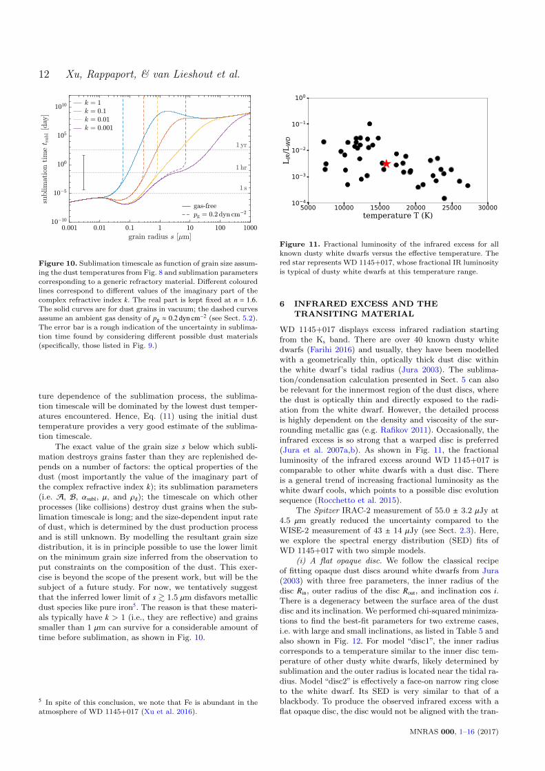
Figure 11. Fractional luminosity of the infrared excess for all

known dusty white dwarfs versus the effective temperature. The

red star represents WD 1145+017, whose fractional IR luminosityis typical of dusty white dwarfs at this temperature range.

6 INFRARED EXCESS AND THETRANSITING MATERIAL

WD 1145+017 displays excess infrared radiation startingfrom the Ks band. There are over 40 known dusty whitedwarfs (Farihi 2016) and usually, they have been modelledwith a geometrically thin, optically thick dust disc withinthe white dwarf’s tidal radius (Jura 2003). The sublima-tion/condensation calculation presented in Sect. 5 can alsobe relevant for the innermost region of the dust discs, wherethe dust is optically thin and directly exposed to the radi-ation from the white dwarf. However, the detailed processis highly dependent on the density and viscosity of the sur-rounding metallic gas (e.g. Rafikov 2011). Occasionally, theinfrared excess is so strong that a warped disc is preferred(Jura et al. 2007a,b). As shown in Fig. 11, the fractionalluminosity of the infrared excess around WD 1145+017 iscomparable to other white dwarfs with a dust disc. Thereis a general trend of increasing fractional luminosity as thewhite dwarf cools, which points to a possible disc evolutionsequence (Rocchetto et al. 2015).

The Spitzer IRAC-2 measurement of 55.0 ± 3.2 µJy at4.5 µm greatly reduced the uncertainty compared to theWISE-2 measurement of 43 ± 14 µJy (see Sect. 2.3). Here,we explore the spectral energy distribution (SED) fits ofWD 1145+017 with two simple models.

(i) A flat opaque disc. We follow the classical recipeof fitting opaque dust discs around white dwarfs from Jura(2003) with three free parameters, the inner radius of thedisc Rin, outer radius of the disc Rout, and inclination cos i.There is a degeneracy between the surface area of the dustdisc and its inclination. We performed chi-squared minimiza-tions to find the best-fit parameters for two extreme cases,i.e. with large and small inclinations, as listed in Table 5 andalso shown in Fig. 12. For model “disc1”, the inner radiuscorresponds to a temperature similar to the inner disc tem-perature of other dusty white dwarfs, likely determined bysublimation and the outer radius is located near the tidal ra-dius. Model “disc2” is effectively a face-on narrow ring closeto the white dwarf. Its SED is very similar to that of ablackbody. To produce the observed infrared excess with aflat opaque disc, the disc would not be aligned with the tran-

MNRAS 000, 1–16 (2017)

A dearth of small particles around WD 1145+017 13

10−1 100 101101

102

103

λ (µm)

F ν(µ

Jy)

u gr

i zY

J

HK

W−1

W−2

I−2

WDWD+Disk1WD+Disk2WD+BB

Figure 12. SED fits of the infrared excess around WD 1145+017.The red square, circle, star, and diamond symbols represent mea-

surement from the SDSS, UKIDSS, WISE, and Spitzer, respec-

tively. The black line represents flux from the white dwarf model.The blue and magenta dashed lines represent flux from an opaque

disc with parameters listed in Table 5 while the blue dashed line

represents flux from a blackbody. The solid coloured lines rep-resent flux from the white dwarf plus an additional component,

either a disc or a blackbody.

siting objects. Under this scenario, either the dust disc andthe transiting objects come from different parent bodies withdifferent orbital inclination, or some additional mechanismis required to perturb the dust disc to be misaligned withthe transiting objects.

(ii) An inflated optically thin disc. The best-fit black-body model has an effective temperature of 1150 K and sur-face area of 160πR2

?, which is consistent with the numbersderived in Vanderburg et al. (2015). This temperature iscomparable to the temperature of large grains around thetransiting material at 1.16R (90 R?), as derived in Eq. (7).To produce the observed infrared excess, a disc height of0.9 R? is required. Collisional cascades around the Roche lim-its of white dwarfs have been studied recently in Kenyon &Bromley (2017). They found for discs made of indestructibleparticles, the scale height would quickly reduce to a valuethat is comparable to the particle radius. However, with ad-ditional mass input, the scale height of the dust disc can re-main quite high for a long time. This is a viable alternativebecause there is a constant mass input from the disintegrat-ing material into the dust disc around WD 1145+017. Inaddition, from the deep transits in the light curve, we knowthat the transiting material has significant height as well.A prediction from this model is that the disc scale heightis dependent on the mass input rate. It is essential to keepmonitoring the infrared flux of the dust disc to look for anyvariations correlated with the transit light curve.

It is worth noting that the transiting material couldcontribute to the infrared excess as well. We approximatethe total effective surface area of the dust as a cylinder andit can be calculated as:

A ≈ 2πr · ε · δ ·√πR? (13)

where ε is the percentage of time a transit lasts, δ is theaverage transit depth, both can be estimated from the lightcurve and

√πR? represents the effective height of the stellar

Table 5. Best-fit parameters to the SED of WD 1145+017

Model χ2d Parameters

disc1 1.3 Rin=13R?, Rout=120R?, cos i = 0.18Tin=1570 K, Tout=300 K

disc2 2.5 Rin=19R?, Rout=25R?, cos i=0.80

Tin=1190 K, Tout=970 KBlackbody 1.3 Tbb=1150 K, A=160πR2

?

Note.

We fit four data points, including fluxes from H, Ks, W-1, and

IRAC-2. χ2d is calculated for per degree of freedom, which is 1

for the opaque disc model and 2 for the blackbody model. For

disc1, the outer radius Rout is not well constrained due to the

lack of longer wavelength observations. We kept it at 120R?, thetypical tidal radius of white dwarfs.

disc. For the 2016 dataset, we found ε = 0.22 and δ= 0.17.For the 2017 dataset, for B2, ε = 0.10, δ = 0.09 while forB3, ε = 0.25, δ=0.33. The total surface area of the tran-siting material is ∼ 12πR2

? and ∼ 29πR2? in 2016 and 2017,

respectively. Thus, there is an increase in surface area by afactor of 2.5 in the 2017 light curve compared to the 2016light curve. However, the surface area of the transiting ma-terial is still relatively small compared to the total inferredsurface area of the emitting dust of 160πR2

?, and the 4.5 µmflux remains constant between 2016 and 2017 observations,requiring a long lasting reservoir of ∼1200 K dust. Regard-less, there could be a significant fraction of non-transitingdust material and the sublimation timescale for large par-ticle is years or longer, as shown in Fig. 10. The transitingobjects could supply material for the observed infrared ex-cess.

7 SUMMARY & CONCLUSION

We have presented two epochs of multi-wavelength photo-metric observations of WD 1145+017, covering from opti-cal to 4.5 µm during 2016 March 28-29 and 2017 April 4-5.One main transit feature was detected in 2016 and threetransit features in 2017 during a 4.5 hr orbital period. Wemodelled the transit features and found that the observedtransit depths were different at all the observed wavelengths.After correcting for the excess infrared emission from orbit-ing dust particles in the Ks and 4.5 µm bands, we foundthat the transit depths are the same from optical to 4.5 µmduring both epochs.

This wavelength-independent transit behaviour can beexplained by a dearth of small grains (. 1.5 µm) in the tran-siting material. Small grains are heated to a higher temper-ature than large grains. In addition, sublimation rates havea steep dependence on grain temperature. As a result, wesuggest a model where small grains sublimate rapidly andonly large grains can survive long enough to be detectable.

The dust released from the hypothesised orbiting bod-ies will continually add mass into the circumstellar dust,which could potentially maintain a large scale height. Wepresent two models that can equally fit the infrared excessof WD 1145+017, including a flat opaque disc and an in-flated optically thin disc. Future observations, particularlymonitoring in the infrared, will improve our understanding

MNRAS 000, 1–16 (2017)

14 Xu, Rappaport, & van Lieshout et al.

of the link between the transiting material and the infraredexcess.

Note Added in Manuscript: After this work was substan-tially complete, we became aware of an interesting model byFarihi et al. (2017) that might explain some of the proper-ties of the peculiar transits in WD 1145+017. This modelinvolves magnetic entrainment of small (a ∼ 0.1 µm) chargedparticles in the field of a strongly magnetised white dwarf.In the context of either the Farihi et al. (2017) scenario, orthe one we have assumed, namely dust clouds released byorbiting bodies with periods near 4.5 hours, all of the mea-sured transit depths and dust size determinations made inthis work should still be equally valid. All of the calculationswe made suggesting that the smaller dust grains should sub-limate quickly would remain unchanged in either scenario.Thus, none of our conclusions should be affected.

ACKNOWLEDGEMENTS

We thank the Spitzer helpdesk for useful discussions abouthigh-precision photometry. The paper was based on obser-vations made with: (i) the Spitzer Space Telescope underprogram #12128 and #13065, which is operated by the JetPropulsion Laboratory, California Institute of Technologyunder a contract with NASA. Support for this work was pro-vided by NASA through an award issued by JPL/Caltech.(ii) the European Organisation for Astronomical Research inthe Southern Hemisphere under ESO programs 296.C-5024and 099.C-0082. This work also makes use of observationsfrom the LCO network. R. van Lieshout acknowledges sup-port from the European Union through ERC grant numbers279973 and 341137. A. Camero acknowledges support fromSTFC grant ST/M001296/1.

REFERENCES

Alonso R., Rappaport S., Deeg H. J., Palle E., 2016, A&A, 589,L6

Backman D. E., Paresce F., 1993, in Levy E. H., Lunine J. I., eds,

Protostars and Planets III. pp 1253–1304

Bohren C. F., Huffman D. R., 1983, Absorption and scattering of

light by small particles

Brinkworth C. S., Gansicke B. T., Marsh T. R., Hoard D. W.,Tappert C., 2009, ApJ, 696, 1402

Brown T. M., et al., 2013, PASP, 125, 1031

Caceres C., et al., 2011, A&A, 530, A5

Collins K., Kielkopf J., 2013, AstroImageJ: ImageJ for Astron-

omy, Astrophysics Source Code Library (ascl:1309.001)

Collins K. A., Kielkopf J. F., Stassun K. G., Hessman F. V., 2017,

AJ, 153, 77

Croll B., et al., 2014, ApJ, 786, 100

Croll B., et al., 2017, ApJ, 836, 82

Dalba P. A., Muirhead P. S., 2016, ApJ, 826, L7

Dalba P. A., Muirhead P. S., Croll B., Kempton E. M.-R., 2017,AJ, 153, 59

Debes J. H., Sigurdsson S., 2002, ApJ, 572, 556

Dufour P., Blouin S., Coutu S., Fortin-Archambault M.,

Thibeault C., Bergeron P., Fontaine G., 2017, in TremblayP.-E., Gaensicke B., Marsh T., eds, Astronomical Society ofthe Pacific Conference Series Vol. 509, 20th European White

Dwarf Workshop. p. 3 (arXiv:1610.00986)

Farihi J., 2016, New Astron. Rev., 71, 9

Farihi J., Jura M., Zuckerman B., 2009, ApJ, 694, 805

Farihi J., von Hippel T., Pringle J. E., 2017, preprint,

(arXiv:1707.09474)

Fazio et al. 2004, ApJS, 154, 10

Gansicke B. T., Marsh T. R., Southworth J., Rebassa-Mansergas

A., 2006, Science, 314, 1908

Gansicke B. T., et al., 2016, ApJ, 818, L7

Gary B. L., Rappaport S., Kaye T. G., Alonso R., Hambschs F.-J.,2017, MNRAS, 465, 3267

Grillmair C. J., et al., 2012, in Observatory Operations:

Strategies, Processes, and Systems IV. p. 84481I,

doi:10.1117/12.927191

Gurri P., Veras D., Gansicke B. T., 2017, MNRAS, 464, 321

Hallakoun N., et al., 2017, MNRAS, 469, 3213

Hansen J. E., Travis L. D., 1974, Space Sci. Rev., 16, 527

Janes K. A., Clemens D. P., Hayes-Gehrke M. N., Eastman J. D.,Sarcia D. S., Bosh A. S., 2004, in American Astronomical

Society Meeting Abstracts #204. p. 672

Jewitt D., 2012, AJ, 143, 66

Jura M., 2003, ApJ, 584, L91

Jura M., 2006, ApJ, 653, 613

Jura M., Young E. D., 2014, Annual Review of Earth and Plan-

etary Sciences, 42, 45

Jura M., Farihi J., Zuckerman B., Becklin E. E., 2007a, AJ, 133,1927

Jura M., Farihi J., Zuckerman B., 2007b, ApJ, 663, 1285

Jura M., Farihi J., Zuckerman B., 2009, AJ, 137, 3191

Kenyon S. J., Bromley B. C., 2017, preprint, (arXiv:1706.08579)

Koester D., Gansicke B. T., Farihi J., 2014, A&A, 566, A34

Langmuir I., 1913, Phys. Rev., 2, 450

Mathis J. S., Rumpl W., Nordsieck K. H., 1977, ApJ, 217, 425

Melis C., Jura M., Albert L., Klein B., Zuckerman B., 2010, ApJ,

722, 1078

Pirard J.-F., Kissler-Patig M., Moorwood, A. et al. 2004, in

Moorwood A. F. M., Iye M., eds, Proc. SPIEVol. 5492,Ground-based Instrumentation for Astronomy. pp 1763–1772,

doi:10.1117/12.578293

Provencal J. L., et al., 2012, ApJ, 751, 91

Rafikov R. R., 2011, MNRAS, 416, L55

Rafikov R. R., Garmilla J. A., 2012, ApJ, 760, 123

Rappaport S., et al., 2012, ApJ, 752, 1

Rappaport S., Barclay T., DeVore J., Rowe J., Sanchis-Ojeda R.,

Still M., 2014, ApJ, 784, 40

Rappaport S., Gary B. L., Kaye T., Vanderburg A., Croll B.,Benni P., Foote J., 2016, MNRAS, 458, 3904

Rappaport S., Gary B. L., Vanderburg A., Xu S., Pooley D.,

Mukai K., 2017, preprint, (arXiv:1709.08195)

Reach W. T., Lisse C., von Hippel T., Mullally F., 2009, ApJ,

693, 697

Redfield S., Farihi J., Cauley P. W., Parsons S. G., Gansicke B. T.,Duvvuri G. M., 2017, ApJ, 839, 42

Rocchetto M., Farihi J., Gansicke B. T., Bergfors C., 2015, MN-

RAS, 449, 574

Vanderburg A., Rappaport S., 2018, Transiting DisintegratingPlanetary Debris around WD 1145+017. Springer

Vanderburg A., et al., 2015, Nature, 526, 546

Veras D., Carter P. J., Leinhardt Z. M., Gansicke B. T., 2017,

MNRAS, 465, 1008

Xu S., Jura M., Dufour P., Zuckerman B., 2016, ApJ, 816, L22

Zhou G., et al., 2016, MNRAS, 463, 4422

Zuckerman B., Koester D., Reid I. N., Hunsch M., 2003, ApJ,596, 477

Zuckerman B., Koester D., Melis C., Hansen B. M., Jura M.,2007, ApJ, 671, 872

Zuckerman B., Melis C., Klein B., Koester D., Jura M., 2010,

ApJ, 722, 725

van Lieshout R., Min M., Dominik C., 2014, A&A, 572, A76

MNRAS 000, 1–16 (2017)

A dearth of small particles around WD 1145+017 15

Figure A1. Observing times for 10 optical sessions in 2017. The

details of the observation are listed in Table A1. The Spitzer and

VLT observing windows are also shown for comparison. The tri-angles indicate phase zero, as defined in the text.

von Hippel T., Kuchner M. J., Kilic M., Mullally F., Reach W. T.,

2007, ApJ, 662, 544

APPENDIX A: OPTICAL LIGHT CURVECOMPARISON

In support of the Spitzer observation on April 4-5, 2017, werequested observing time in ten optical telescopes all aroundthe world. These 10 ground-based light curves offer a uniqueopportunity for assessing the level of systematics that can beexpected in any single light curve. The observations are sum-marised in Table A1. These 10 observing sessions spanned26 hours, or ∼ 6 WD 1145+017 orbital periods, as shown inFig. A1.

Most of the data were reduced with AstroImageJ,an open software for high-precision light curve extrapola-tions (Collins & Kielkopf 2013; Collins et al. 2017). TheLas Cumbres Observatory (LCO) data were reduced follow-ing previous procedures developed for LCO observations ofWD 1145+017 outlined in Zhou et al. (2016). The data re-duction procedures for the JBO and HAO observations weredescribed in Rappaport et al. (2016). The Perkins observa-tions were described in detail in Sect. 2.1. All the light curvesare shown in Figs A2 and A3, also shown is the best-fit modelfor the Perkins data.

There are three main dip features in an orbital period,which we name B1, B2, and B3, respectively. Since the tran-sits around WD 1145+017 change gradually, any noticeablechange typically occurs on a longer timescale than an orbitalperiod. We consider the first 3 light curves as close enoughin time to justify a direct comparison. The last 7 light curvesare simultaneous. We will refer to those two groups as ‘earlygroup’ and ‘late group’.

The early group of light curves were all obtained withthe 1-m LCO network (Brown et al. 2013). The variationsamong the light curves suggest that systematic plus stochas-tic differences amount to ∼ 2.5% for these data for a cadence∼ 220 s. B1 has a depth about 2.7% (see Table 2), and it wasnot detected in the LCO light curve. For the late group, thePerkins data have the best quality followed by the FLWOKeplerCam data.

As shown in Figs A2 and A3, the overall agreement is

0.4

0.6

0.8

1.0

LCO

-coj

0.4

0.6

0.8

1.0

LCO

-cpt B1

B2

B3

0.0 0.2 0.4 0.6 0.8 1.0Phase

0.4

0.6

0.8

1.0

LCO

-lsc

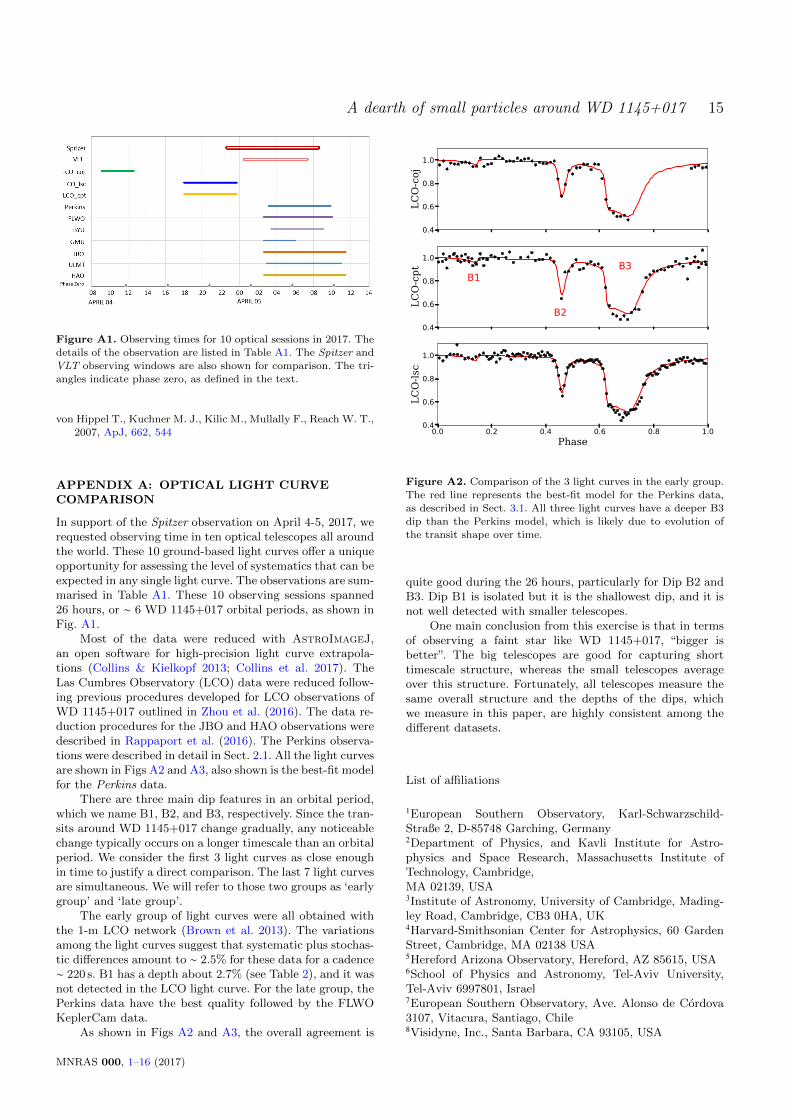
Figure A2. Comparison of the 3 light curves in the early group.

The red line represents the best-fit model for the Perkins data,

as described in Sect. 3.1. All three light curves have a deeper B3dip than the Perkins model, which is likely due to evolution of

the transit shape over time.

quite good during the 26 hours, particularly for Dip B2 andB3. Dip B1 is isolated but it is the shallowest dip, and it isnot well detected with smaller telescopes.

One main conclusion from this exercise is that in termsof observing a faint star like WD 1145+017, “bigger isbetter”. The big telescopes are good for capturing shorttimescale structure, whereas the small telescopes averageover this structure. Fortunately, all telescopes measure thesame overall structure and the depths of the dips, whichwe measure in this paper, are highly consistent among thedifferent datasets.

List of affiliations

1European Southern Observatory, Karl-Schwarzschild-Straße 2, D-85748 Garching, Germany2Department of Physics, and Kavli Institute for Astro-physics and Space Research, Massachusetts Institute ofTechnology, Cambridge,MA 02139, USA3Institute of Astronomy, University of Cambridge, Mading-ley Road, Cambridge, CB3 0HA, UK4Harvard-Smithsonian Center for Astrophysics, 60 GardenStreet, Cambridge, MA 02138 USA5Hereford Arizona Observatory, Hereford, AZ 85615, USA6School of Physics and Astronomy, Tel-Aviv University,Tel-Aviv 6997801, Israel7European Southern Observatory, Ave. Alonso de Cordova3107, Vitacura, Santiago, Chile8Visidyne, Inc., Santa Barbara, CA 93105, USA

MNRAS 000, 1–16 (2017)

16 Xu, Rappaport, & van Lieshout et al.

Table A1. Summary of Optical Observations on April 4-5, 2017

Telescope Name Location Aperture Observers Cadence Filters

Early Group

LCO/COJ SSO, Australia 1m Avi Shporer 221s g

LCO/LSC CTIO, Chile 1m Avi Shporer 219s gLCO/CPT SAAO, South Africa 1m Avi Shporer 220s g

Late GroupPerkins Lowell, AZ 1.8m Paul Dalba 51s R

FLWO FLWO, AZ 1.2m Allyson Bieryla 77s V

BYU West Mountain Observatory, UT 0.91m Michael Joner 190s VGMU Fairfax, VA 0.81m Jenna Cann, Peter A. Panka 133s Clear

JBO Hereford, AZ 0.81m Tom Kaye 58s Clear

ULMT Mt. Lemmon, AZ 0.6m Karen Collins 213s ClearHAO Hereford, AZ 0.35m Bruce Gary 87s Clear

0.50

0.75

1.00

Perk

ins

0.50

0.75

1.00

FLW

O

0.50

0.75

1.00

BYU B1

B2

B3

0.50

0.75

1.00

GM

U

0.50

0.75

1.00

JBO

0.50

0.75

1.00

ULM

T

0.0 0.2 0.4 0.6 0.8 1.0Phase

0.50

0.75

1.00

HAO

Figure A3. Comparison of the 7 light curves in the late group.

The red line represents the best-fit model for the Perkins data,as described in Sect. 3.1.

9Observatoire Astronomique de l’Universit’e de Geneve, 51ch. des Maillettes, 1290 Versoix, Switzerland10Research School of Astronomy and Astrophysics, MountStromlo Observatory, Australian National University,Weston, ACT 2611, Australia11Centre for Exoplanet Science, SUPA School of Physics &Astronomy , University of St Andrews, North Haugh, STANDREWS KY16 9SS, UK12Department of Physics and Astronomy, George Mason

University, Fairfax, Virginia, USA (GMU observations)13Institute for Astrophysical Research, Boston University,725 Commonwealth Avenue, Room 506, Boston, MA 02215,USA14Space Telescope Science Institute, Baltimore, MD 21218,USA15Paul & Jane Meyer Observatory, Coryell County, TX16Institut de Recherche sur les Exoplanetes (iREx) and De-partement de physique, Universite de Montreal, Montreal,QC H3C 3J7, Canada17Eureka Scientific Inc., Oakland, CA, USA 9460218Instituto de Astrofısica, Facultad de Fısica, PontificiaUniversidad Catolica de Chile, Av. Vicuna Mackenna 4860,782-0436 Macul,Santiago, Chile19Department of Physics and Astronomy, Brigham YoungUniversity, Provo, UT 84602, USA(BYU observations)20Department of Physics and Astronomy, University ofCalifornia, Los Angeles, CA 90095-1562, USA21Raemor Vista Observatory, 7023 E. Alhambra Dr., SierraVista, AZ 85650, USA (JBO observations)22Temple College, Temple, TX, 7650423Instituto de Astrofısica de Canarias, Vıa Lactea s/n,E-38205 La Laguna, Tenerife, Spain24Departamento de Astrofısica, Universidad de La Laguna,Spain25Department of Physics and Astronomy, University ofDelaware, Newark, DE 19716, USA26Ramotholo Sefako, South African Astronomical Observa-tory, PO Box 9, Observatory, 7935, South Africa27Division of Geological and Planetary Sciences, CaliforniaInstitute of Technology, Pasadena, CA 91125, USA

This paper has been typeset from a TEX/LATEX file prepared by

the author.

MNRAS 000, 1–16 (2017)