arithmetic aspects of random walks and methods in definite
TRANSCRIPT

Arithmetic aspects of random walksand methods in definite integration
An Abstract
Submitted On The First Day Of May, 2012
To The Department Of Mathematics
In Partial Fulfillment Of The Requirements
Of The School Of Science And Engineering
Of Tulane University
For The Degree Of
Doctor Of Philosophy
By
Armin Straub
Approved:Victor H. Moll, Ph.D.
Director
Tewodros Amdeberhan, Ph.D.
Jonathan M. Borwein, D.Phil.
Mahir B. Can, Ph.D.
Morris Kalka, Ph.D.

Abstract
In the first part of this thesis, we revisit a classical problem: how far does a random
walk travel in a given number of steps (of length 1, each taken along a uniformly
random direction)? We study the moments of the distribution of these distances
as well as the corresponding probability distributions. Although such random walks
are asymptotically well understood, very few exact formulas had been known; we
supplement these with explicit hypergeometric forms and unearth general structures.
Our investigation of the moments naturally leads us to consider (multiple) Mahler
measures. For several families of Mahler measures we are able to give evaluations in
terms of log-sine integrals. Therefore, and because of the connections of log-sine
integrals with number theory and mathematical physics, we study generalized log-
sine integrals and show that they evaluate in terms of the well-studied polylogarithms.
A computer algebra implementation of our results demonstrates that a large body of
results on log-sine integrals scattered over the literature is now computer-amenable.
The second part is concerned with developing specific methods for evaluating
several families of definite integrals arising in diverse contexts (such as calculations in
quantum field theories). We also review and illustrate Ramanujan’s Master Theorem
and show that it generalizes to the method of brackets, which has its roots in the
negative dimensional integration method utilized by particle physicists. We then
apply this technique to multiple integrals recently studied in a physical context.
Complementary to these symbolic methods, we present an exponentially fast algo-
rithm for numerically integrating rational functions over the real line. This algorithm
operates on the coefficients of the rational function instead of evaluating it.

Arithmetic aspects of random walksand methods in definite integration
A Dissertation
Submitted On The First Day Of May, 2012
To The Department Of Mathematics
In Partial Fulfillment Of The Requirements
Of The School Of Science And Engineering
Of Tulane University
For The Degree Of
Doctor Of Philosophy
By
Armin Straub
Approved:Victor H. Moll, Ph.D.
Director
Tewodros Amdeberhan, Ph.D.
Jonathan M. Borwein, D.Phil.
Mahir B. Can, Ph.D.
Morris Kalka, Ph.D.


Acknowlegdment
Let me begin by thanking my collaborators and coauthors who have directly con-
tributed to the work presented in this thesis:
• Tewodros Amdeberhan (Tulane University),
• David Borwein (University of Western Ontario),
• Jonathan M. Borwein (University of Newcastle, Australia),
• Olivier Espinosa (then Universidad Tecnica Federico Santa Marıa, Chile),
• Ivan Gonzalez (Universidad Tecnica Federico Santa Marıa, Chile),
• Marshall Harrison (Prestadigital LLC, Texas),
• Dante Manna (then Virginia Wesleyan College),
• Luis Medina (then Rutgers University),
• Victor H. Moll (Tulane University),
• Dirk Nuyens (K.U.Leuven, Belgium),
• James Wan (University of Newcastle, Australia), and
• Wadim Zudilin (University of Newcastle, Australia).
You have shown me that the beautiful and exciting land of mathematics is most
enjoyably explored in company and with guidance. All the papers presented in this
thesis, with the exception of the ones in Chapters 15 and 16, have been worked out
with at least one coauthor.
I am particularly grateful to my advisor Victor Moll who has always been an
unfailing source of energy and support. Victor is full of ideas and advice, and has
the gift of getting you hooked on interesting problems which he naturally attracts.
ii

Also, his ability to remember and come up with relevant references is remarkable and
has been very useful to me. Victor is a pleasure to work with and the main reason I
returned to Tulane to pursue a doctoral degree.
Tewodros Amdeberhan is one of the most enthusiastic and friendly persons I
have met. His enormous enthusiasm, encouragement and curiosity have supported
me throughout my times at Tulane. Early on, Teddy engaged me in mathematical
research and my first publication [Str08], presented in Chapter 15, is owed to his
encouragement. I am much indebted for his support, occasionally shared over a cup
of coffee, as a mentor and friend.
It was most fortunate for me, both mathematically and personally, to have had
the opportunity to visit Jonathan Borwein at Newcastle University. His industrious
and resourceful character continue to have a contagious effect on me, which makes
our collaboration not only fruitful but very enjoyable. I also thank Jon and his wife
Judith for several cultural and culinary introductions to Australia.
At Newcastle University, I have further benefited considerably from the presence
of James Wan and Wadim Zudilin. James, a fellow graduate student, is full of in-
triguing thoughts, both mathematical and philosophical. I have enjoyed his company
immensely and am fond to recall our excursions in Newcastle, Vancouver and San
Francisco. I am very thankful to Wadim, a true scholar, for sharing his remarkable
mathematical knowledge on many occasions. His interest and his friendly support
have been a delight.
I also wish to thank Manuel Kauers and Christoph Koutschan from RISC for sev-
eral helpful discussions on applications of computer algebra. In particular, Christoph’s
package HolonomicFunctions, [Kou10], has been most helpful as has been his advice
on using it.
More specifically, the work in Chapter 2 benefited from helpful suggestions by
David Bailey, David Broadhurst and Richard Crandall. Further thanks are due to
iii
Bruno Salvy for reminding us of the existence of [Bar64], Michael Mossinghoff for
showing us [Klu06], and to Peter Donovan for stimulating the research on random
walks and for much subsequent useful discussion. We are grateful to Wadim Zudilin
for much useful discussion on the work in Chapter 3, as well as for pointing out [Bai32],
[Nes03], and [Zud02], which have been crucial in obtaining the closed forms ofW4(±1).
We thank Michael Mossinghoff for pointing us to the Mahler measure conjectures via
[RVTV04], and Plamen Djakov and Boris Mityagin for correspondence related to
Theorem 4.2.7 and the history of their proof. We are specially grateful to Don Zagier
for not only providing us with his proof of Theorem 4.2.7 but also for his enormous
amount of helpful comments which improved Chapter 4. We are much obliged to
David Bailey for significant numerical assistance in Chapters 4 and 7, especially with
the two-dimensional quadratures in Example 7.9.2. Thanks are due to Yasuo Ohno
and Yoshitaka Sasaki for introducing us to the relevant papers introducing multiple
and higher Mahler measure during a visit to CARMA. This initiated the work in
Chapters 6 and 7. Chapter 6 benefited from many useful discussions with James Wan
and David Borwein. We are grateful to Andrei Davydychev and Mikhail Kalmykov
for several valuable comments on an earlier version of work presented in Chapter 5
and for pointing us to relevant publications. We also wish to thank Bruce Berndt
for pointing out the results described in Section 12.8 of Chapter 12. Chapter 13 was
improved by Larry Glasser who pointed us to the sinc integral problem after hearing
a lecture on [BB01] and who provided historic context. We are also thankful for his
and Tewodros Amdeberhan’s comments on an earlier draft of the work in Chapter 13.
The topic of Chapter 15 was suggested by Tewodros Amdeberhan and I am especially
thankful for his continuous and helpful support on this subject. I also appreciate the
help received by Doron Zeilberger who shared his expertise in the form of useful Maple
routines. Most parts of Chapter 16 have been written while I had the pleasure to
visit Marc Chamberland at Grinnell College. I am thankful for his encouraging and
iv
helpful support.
Throughout my time as a graduate student I have received gracious financial
support from various sources. As a graduate student, I was funded by teaching assis-
tantships, fellowship awards and tuition scholarships awarded by Tulane University
for the years 2006/2007 and 2008–2012. As a student of Victor Moll, I was also
supported by the NSF grants NSF-DMS 0070567, NSF-DMS 0070757, NSF-DMS
0409968, and NSF-DMS 0713836. During the academic year 2009/2010 I received
support as an IBM Fellow in Computational Science. The three visits at Newcastle
University were generously funded by Jonathan Borwein with support from the Aus-
tralian Research Council. Attending the conferences FPSAC 2009, 2010, 2011 as well
as the AMS Joint Meetings 2012 was made possible by kind travel support from the
NSF.
Finally, I wish to thank Victor Moll, Tewodros Amdeberhan, Jonathan Borwein,
Mahir Can and Morris Kalka for serving on my dissertation committee.
v
Table of Contents
Acknowledgement ii
1 Introduction and overview 1
1.1 Overview . . . . . . . . . . . . . . . . . . . . . . . . . . . . . . . . 1
1.2 Arithmetic aspects of random walks . . . . . . . . . . . . . . . . . 4
1.3 Methods in definite integration . . . . . . . . . . . . . . . . . . . . 7
1.4 Some notation . . . . . . . . . . . . . . . . . . . . . . . . . . . . . 9
2 Some arithmetic properties of short random walk integrals 12
2.1 Introduction, history and preliminaries . . . . . . . . . . . . . . . 13
2.2 The even moments and their combinatorial features . . . . . . . . 18
2.3 Analytic features of the moments . . . . . . . . . . . . . . . . . . 25
2.4 Bessel integral representations . . . . . . . . . . . . . . . . . . . . 31
2.5 The odd moments of a three-step walk . . . . . . . . . . . . . . . 32
2.6 Appendix . . . . . . . . . . . . . . . . . . . . . . . . . . . . . . . 37
vi
3 Three-step and four-step random walk integrals 43
3.1 Introduction and preliminaries . . . . . . . . . . . . . . . . . . . . 43
3.2 Bessel integral representations . . . . . . . . . . . . . . . . . . . . 46
3.3 Probabilistically inspired representations . . . . . . . . . . . . . . 60
3.4 Partial resolution of Conjecture 3.1.1 . . . . . . . . . . . . . . . . 69
4 Densities of short uniform random walks 73
4.1 Introduction . . . . . . . . . . . . . . . . . . . . . . . . . . . . . . 73
4.2 The densities pn . . . . . . . . . . . . . . . . . . . . . . . . . . . . 76
4.3 The density p3 . . . . . . . . . . . . . . . . . . . . . . . . . . . . . 82
4.4 The density p4 . . . . . . . . . . . . . . . . . . . . . . . . . . . . . 84
4.5 The density p5 . . . . . . . . . . . . . . . . . . . . . . . . . . . . . 92
4.6 Derivative evaluations of Wn . . . . . . . . . . . . . . . . . . . . . 97
4.7 New results on the moments Wn . . . . . . . . . . . . . . . . . . . 104
4.8 Appendix: A family of combinatorial identities . . . . . . . . . . . 110
5 Special values of generalized log-sine integrals 114
5.1 Introduction . . . . . . . . . . . . . . . . . . . . . . . . . . . . . . 115
5.2 Evaluations at π . . . . . . . . . . . . . . . . . . . . . . . . . . . . 117
5.3 Quasiperiodic properties . . . . . . . . . . . . . . . . . . . . . . . 125
5.4 Evaluations at other values . . . . . . . . . . . . . . . . . . . . . . 127
5.5 Reducing polylogarithms . . . . . . . . . . . . . . . . . . . . . . . 134
5.6 The program . . . . . . . . . . . . . . . . . . . . . . . . . . . . . . 136
vii

6 Log-sine evaluations of Mahler measures 139
6.1 Preliminaries . . . . . . . . . . . . . . . . . . . . . . . . . . . . . . 139
6.2 Log-sine integrals at π and π/3 . . . . . . . . . . . . . . . . . . . 142
6.3 Log-sine evaluations of multiple Mahler measures . . . . . . . . . 152
6.4 Moments of random walks . . . . . . . . . . . . . . . . . . . . . . 156
6.5 Conclusion . . . . . . . . . . . . . . . . . . . . . . . . . . . . . . . 165
7 Log-sine evaluations of Mahler measures, II 167
7.1 Introduction . . . . . . . . . . . . . . . . . . . . . . . . . . . . . . 167
7.2 Preliminaries . . . . . . . . . . . . . . . . . . . . . . . . . . . . . . 169
7.3 Log-sine integrals . . . . . . . . . . . . . . . . . . . . . . . . . . . 169
7.4 Mahler measures and moments of random walks . . . . . . . . . . 175
7.5 Epsilon expansion of W3 . . . . . . . . . . . . . . . . . . . . . . . 177
7.6 Trigonometric analysis of µn(1 + x+ y) . . . . . . . . . . . . . . . 182
7.7 Explicit evaluations of µn(1 + x+ y) for small n . . . . . . . . . . 195
7.8 Proofs of two conjectures of Boyd . . . . . . . . . . . . . . . . . . 201
7.9 Conclusion . . . . . . . . . . . . . . . . . . . . . . . . . . . . . . . 204
8 Ramanujan’s Master Theorem 206
8.1 Introduction . . . . . . . . . . . . . . . . . . . . . . . . . . . . . . 206
8.2 History . . . . . . . . . . . . . . . . . . . . . . . . . . . . . . . . . 208
8.3 Rigorous treatment of the Master Theorem . . . . . . . . . . . . . 211
viii

8.4 A collection of elementary examples . . . . . . . . . . . . . . . . . 212
8.5 A quartic integral . . . . . . . . . . . . . . . . . . . . . . . . . . . 216
8.6 Random walk integrals . . . . . . . . . . . . . . . . . . . . . . . . 218
8.7 Extending the domain of validity . . . . . . . . . . . . . . . . . . 220
8.8 Some classical polynomials . . . . . . . . . . . . . . . . . . . . . . 221
8.9 The method of brackets . . . . . . . . . . . . . . . . . . . . . . . . 225
9 The method of brackets. Part 2: Examples and applications 232
9.1 Introduction . . . . . . . . . . . . . . . . . . . . . . . . . . . . . . 232
9.2 The method of brackets . . . . . . . . . . . . . . . . . . . . . . . . 234
9.3 An example from Gradshteyn and Ryzhik . . . . . . . . . . . . . . 236
9.4 Integrals of the Ising class . . . . . . . . . . . . . . . . . . . . . . 238
9.5 Analytic continuation of hypergeometric functions . . . . . . . . . 248
9.6 Feynman diagram application . . . . . . . . . . . . . . . . . . . . 251
9.7 Conclusions and future work . . . . . . . . . . . . . . . . . . . . . 255
10 A fast numerical algorithm for the integration of rational functions 256
10.1 Introduction . . . . . . . . . . . . . . . . . . . . . . . . . . . . . . 257
10.2 The Landen transformation . . . . . . . . . . . . . . . . . . . . . 260
10.3 Complexity of the algorithm . . . . . . . . . . . . . . . . . . . . . 265
10.4 Some numerical examples . . . . . . . . . . . . . . . . . . . . . . . 267
10.5 Convergence of Landen iterates . . . . . . . . . . . . . . . . . . . 269
10.6 Implementation . . . . . . . . . . . . . . . . . . . . . . . . . . . . 277
10.7 Conclusions . . . . . . . . . . . . . . . . . . . . . . . . . . . . . . 281
ix

11 Closed-form evaluation of integrals appearing in positronium decay 282
11.1 Introduction . . . . . . . . . . . . . . . . . . . . . . . . . . . . . . 282
11.2 Some logarithmic integrals . . . . . . . . . . . . . . . . . . . . . . 285
11.3 A trigonometric integral . . . . . . . . . . . . . . . . . . . . . . . 287
11.4 Application to the positronium decay integrals . . . . . . . . . . . 288
12 Wallis-Ramanujan-Schur-Feynman 291
12.1 Wallis’ infinite product for π . . . . . . . . . . . . . . . . . . . . . 292
12.2 A rational integral and its trigonometric version . . . . . . . . . . 293
12.3 A squeezing method . . . . . . . . . . . . . . . . . . . . . . . . . . 296
12.4 An example of Ramanujan and a generalization . . . . . . . . . . 297
12.5 Representation in terms of Schur functions . . . . . . . . . . . . . 300
12.6 Schur functions in terms of SSYT . . . . . . . . . . . . . . . . . . 304
12.7 A counting problem . . . . . . . . . . . . . . . . . . . . . . . . . . 305
12.8 An integral from Gradshteyn and Ryzhik . . . . . . . . . . . . . . 306
12.9 A sum related to Feynman diagrams . . . . . . . . . . . . . . . . 308
12.10 Conclusions . . . . . . . . . . . . . . . . . . . . . . . . . . . . . . 312
13 A sinc that sank 313
13.1 Introduction and background . . . . . . . . . . . . . . . . . . . . . 313
13.2 Evaluation of In . . . . . . . . . . . . . . . . . . . . . . . . . . . . 316
13.3 The case n = 3 . . . . . . . . . . . . . . . . . . . . . . . . . . . . 322
x

13.4 Especially special cases of sinc integrals . . . . . . . . . . . . . . . 327
13.5 The case n > 4 . . . . . . . . . . . . . . . . . . . . . . . . . . . . 332
13.6 Conclusions . . . . . . . . . . . . . . . . . . . . . . . . . . . . . . 334
14 The p-adic valuation of k-central binomial coefficients 336
14.1 Introduction . . . . . . . . . . . . . . . . . . . . . . . . . . . . . . 336
14.2 The integrality of c(n, k) . . . . . . . . . . . . . . . . . . . . . . . 339
14.3 The valuation of c(n, k) . . . . . . . . . . . . . . . . . . . . . . . . 342
14.4 A q-generalization of c(n, k) . . . . . . . . . . . . . . . . . . . . . 347
14.5 Future directions . . . . . . . . . . . . . . . . . . . . . . . . . . . 348
15 Positivity of Szego’s rational function 352
15.1 Introduction . . . . . . . . . . . . . . . . . . . . . . . . . . . . . . 353
15.2 Positivity preserving operations . . . . . . . . . . . . . . . . . . . 354
15.3 Szego’s rational function . . . . . . . . . . . . . . . . . . . . . . . 356
15.4 On positivity of a family of rational functions . . . . . . . . . . . 360
16 A q-analog of Ljunggren’s binomial congruence 366
16.1 Introduction and notation . . . . . . . . . . . . . . . . . . . . . . 366
16.2 A bit of history . . . . . . . . . . . . . . . . . . . . . . . . . . . . 368
16.3 A q-analog of Ljunggren’s congruence . . . . . . . . . . . . . . . . 369
16.4 A q-analog of Wolstenholme’s congruence . . . . . . . . . . . . . . 371
xi

17 Outlook 374
17.1 The method of brackets and similar approaches . . . . . . . . . . 374
17.2 Creative telescoping leading to divergent integrals . . . . . . . . . 387
Bibliography 392
xii

1
Chapter 1
Introduction and overview
1.1 Overview
All but the first and last chapters of this thesis correspond to a paper that either
has already appeared for publication or which has been accepted for publication.
The work presented in Chapters 2–7 originated from revisiting the classical prob-
lem of how far a planar random walk travels in a given number of steps. A summary
and introduction is given in Section 1.2. We record here an overview of these chapters:
Chapter 2: [BNSW11] Some arithmetic properties of short random walk integrals(with Jonathan M. Borwein, Dirk Nuyens, James Wan)
published in The Ramanujan Journal, Vol. 26, Nr. 1, 2011, p. 109-132
Chapter 3: [BSW11] Three-step and four-step random walk integrals(with Jonathan M. Borwein, James Wan)
to appear in Experimental Mathematics
Chapter 4: [BSWZ11] Densities of short uniform random walks(with Jonathan M. Borwein, James Wan, Wadim Zudilin (appendix by Don Zagier))
to appear in Canadian Journal of Mathematics
Chapter 5: [BS11c] Special values of generalized log-sine integrals(with Jonathan M. Borwein)
published in Proceedings of ISSAC 2011 (36th International Symposium on Symbolic and
Algebraic Computation), ACM Press, Jun 2011, p. 43-50
— received ISSAC 2011 Distinguished Student Author Award

2
Chapter 6: [BS11a] Log-sine evaluations of Mahler measures(with Jonathan M. Borwein)
to appear in Journal of the Australian Mathematical Society
Chapter 7: [BBSW12] Log-sine evaluations of Mahler measures, part II(with David Borwein, Jonathan M. Borwein, James Wan)
to appear in Integers (Selfridge memorial volume)
Chapters 8–13 are concerned with developing specific methods for evaluating sev-
eral families of definite integrals arising in diverse contexts (such as calculations in
quantum field theories). An introduction to this second part is given in Section 1.3.
Again, we record the relevant chapters:
Chapter 8: [AEG+11] Ramanujan’s Master Theorem(with Tewodros Amdeberhan, Ivan Gonzalez, Marshall Harrison, Victor H. Moll)
to appear in The Ramanujan Journal
Chapter 9: [GMS10] The method of brackets. Part 2: Examples and applications(with Ivan Gonzalez, Victor H. Moll)
published in “Gems in Experimental Mathematics”, Contemporary Mathematics, Vol. 517,
2010, p. 157-171
Chapter 10: [MMMS10] A fast numerical algorithm for the integration of rationalfunctions(with Dante Manna, Luis Medina, Victor H. Moll)
published in Numerische Mathematik, Vol. 115, Nr. 2, Apr 2010, p. 289-307
Chapter 11: [AMS09] Closed-form evaluation of integrals appearing in positroniumdecay(with Tewodros Amdeberhan, Victor H. Moll)
published in Journal of Mathematical Physics, Vol. 50, Nr. 10, Oct 2009, 6 p.
Chapter 12: [AEMS10] Wallis-Ramanujan-Schur-Feynman(with Tewodros Amdeberhan, Olivier Espinosa, Victor H. Moll)
published in American Mathematical Monthly, Vol. 117, Nr. 15, Aug 2010, p. 618-632
Chapter 13: [BBS12] A sinc that sank(with David Borwein, Jonathan M. Borwein)
to appear in American Mathematical Monthly, Vol. 119, Nr. 7, Aug-Sep 2012
Finally, this thesis includes Chapters 14, 15 and 16 which discuss work of a more
combinatorial type.

3
In Chapter 14 we study the divisibility properties of the coefficients c(n, k) defined
by
(1− k2x)−1/k =∑n≥0
c(n, k)xn
which generalize the central binomial coefficients c(n, 2) =(
2nn
). In particular, we
show that the coefficients are integers.
In Chapter 15 we consider the problem of deciding whether a given rational func-
tion has a power series expansion of entirely positive coefficients. By introducing an
elementary transformation that preserves such positivity we prove the positivity of
1
(1− x)(1− y) + (1− y)(1− z) + (1− z)(1− x),
which goes back at least to Gabor Szego. We then consider applications of this
transformation to more general classes of rational functions.
Chapter 16 establishes a q-analog of the classical binomial congruence
(ap
bp
)≡(a
b
)mod p3,
where p > 3 is a prime. This resolves a problem posed by George Andrews in [And99].
Chapter 14: [SMA09] The p-adic valuation of k-central binomial coefficients(with Tewodros Amdeberhan, Victor H. Moll)
published in Acta Arithmetica, Vol. 140, 2009, p. 31-42
Chapter 15: [Str08] Positivity of Szego’s rational functionpublished in Advances in Applied Mathematics, Vol. 41, Issue 2, Aug 2008, p. 255-264
Chapter 16: [Str11] A q-analog of Ljunggren’s binomial congruencepublished in DMTCS Proceedings: 23rd International Conference on Formal Power Series and
Algebraic Combinatorics (FPSAC), Jun 2011, p. 897-902

4
1.2 Arithmetic aspects of random walks
An n-step uniform random walk starts at the origin of the plane and consists of
n steps of length 1, each taken into a uniformly random direction. The study of such
walks largely originated with Pearson more than a century ago [Pea05a]. He posed
the problem of determining the distribution of the distance from the origin after a
certain number, say n, of steps. Let Wn(s) denote the sth moment of this distance
and pn the corresponding probability density function. Starting with the integral
representation
Wn(s) =
∫ 1
0
. . .
∫ 1
0
∣∣∣∣∣n∑k=1
e2πitk
∣∣∣∣∣s
dt1 · · · dtn (1.1)
the moments are studied in detail in Chapters 2 and 3. It is shown that the even
moments have the interesting combinatorial evaluation
Wn(2k) =∑
a1+···+an=k
(k
a1, . . . , an
)2
. (1.2)
The consequent recurrences satisfied by the even moments are lifted to functional
equations satisfied by Wn(s). In the cases n = 3 and n = 4 a more explicit study
shows that Wn(s) has a representation as a Meijer G-function. Ultimately, using
transformations of Meijer G-functions and identities from the theory of elliptic in-
tegrals, this allows us to find closed formulas for the average distances W3(1) and
W4(1) (in the latter case, as a sum of 6F5’s). Previously, only the trivial evaluation
W2(1) = 4π
was known.
Knowledge of the pole structure of the Wn(s) and the general theory of the (distri-
butional) Mellin calculus allow us to prove in Chapter 4 that the densities pn satisfy
Fuchsian differential equations. Using a family of combinatorial identities discovered
in [DM04] (Don Zagier kindly provided his direct combinatorial proof as an appendix
to Chapter 4) we show that the singularities of pn occur at the positive integers
5
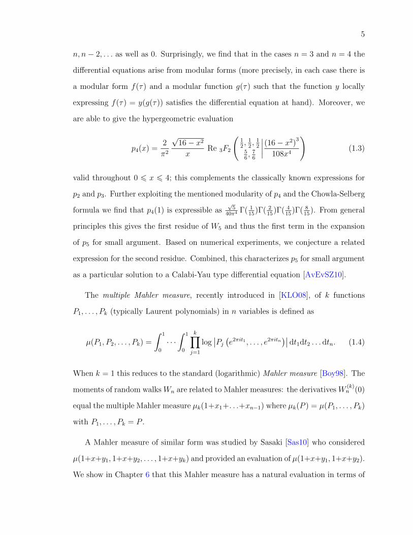
n, n− 2, . . . as well as 0. Surprisingly, we find that in the cases n = 3 and n = 4 the
differential equations arise from modular forms (more precisely, in each case there is
a modular form f(τ) and a modular function g(τ) such that the function y locally
expressing f(τ) = y(g(τ)) satisfies the differential equation at hand). Moreover, we
are able to give the hypergeometric evaluation
p4(x) =2
π2
√16− x2
xRe 3F2
(12, 1
2, 1
256, 7
6
∣∣∣∣(16− x2)3
108x4
)(1.3)
valid throughout 0 6 x 6 4; this complements the classically known expressions for
p2 and p3. Further exploiting the mentioned modularity of p4 and the Chowla-Selberg
formula we find that p4(1) is expressible as√
540π4 Γ( 1
15)Γ( 2
15)Γ( 4
15)Γ( 8
15). From general
principles this gives the first residue of W5 and thus the first term in the expansion
of p5 for small argument. Based on numerical experiments, we conjecture a related
expression for the second residue. Combined, this characterizes p5 for small argument
as a particular solution to a Calabi-Yau type differential equation [AvEvSZ10].
The multiple Mahler measure, recently introduced in [KLO08], of k functions
P1, . . . , Pk (typically Laurent polynomials) in n variables is defined as
µ(P1, P2, . . . , Pk) =
∫ 1
0
· · ·∫ 1
0
k∏j=1
log∣∣Pj (e2πit1 , . . . , e2πitn
)∣∣ dt1dt2 . . . dtn. (1.4)
When k = 1 this reduces to the standard (logarithmic) Mahler measure [Boy98]. The
moments of random walks Wn are related to Mahler measures: the derivatives W(k)n (0)
equal the multiple Mahler measure µk(1+x1+. . .+xn−1) where µk(P ) = µ(P1, . . . , Pk)
with P1, . . . , Pk = P .
A Mahler measure of similar form was studied by Sasaki [Sas10] who considered
µ(1+x+y1, 1+x+y2, . . . , 1+x+yk) and provided an evaluation of µ(1+x+y1, 1+x+y2).
We show in Chapter 6 that this Mahler measure has a natural evaluation in terms of

6
log-sine integrals. Namely, if
Ls(k)n (σ) = −
∫ σ
0
θk logn−1−k∣∣∣∣2 sin
θ
2
∣∣∣∣ dθ (1.5)
denotes the (generalized) log-sine integral then
µ(1 + x+ y1, . . . , 1 + x+ yk) =1
πLsk+1
(π3
)− 1
πLsk+1 (π) . (1.6)
In Chapters 6 and 7 we demonstrate that several other Mahler measures have values
involving generalized log-sine integrals at π, π/3 or more general arguments. Accord-
ingly, we analyze in Chapter 5 log-sine integrals and their evaluations, both explicit
and in terms of generating series. We show that log-sine integrals can be systemati-
cally evaluated in terms of polylogarithms of Nielsen type at corresponding argument.
This approach unifies (and automatizes) various results found in the literature (and
rectifies several errors; see Chapter 5 and [BS11b]). The implementation of our re-
sults in the computer algebra systems SAGE and Mathematica complements existing
computer algebra packages such as lsjk [KS05] for numerical evaluations of log-sine
integrals, or HPL [Mai06] as well as [VW05] for working with multiple polylogarithms.
These packages are used, for instance, in particle physics [DK00, KV00] where log-
sine integrals appeared in recent work on the higher-order terms in the ε-expansion
of various Feynman diagrams.

7
1.3 Methods in definite integration
Many families of definite integrals can be evaluated using Ramanujan’s Master
Theorem (RMT, henceforth)
∫ ∞0
xs−1
{λ(0)− x
1!λ(1) +
x2
2!λ(2)− · · ·
}dx = Γ(s)λ(−s). (1.7)
As an application we show in Chapter 8 that David Broadhurst’s Bessel integral rep-
resentation [Bro09] of the moments Wn(s) of random walks can be derived naturally:
Wn(s) = 2s+1−k Γ(1 + s2)
Γ(k − s2)
∫ ∞0
x2k−s−1
(−1
x
d
dx
)kJn0 (x) dx (1.8)
for 2k > Re s > max(−2,−n2). Moreover, we demonstrate that RMT can be used
to explain the method of brackets, a method for evaluating multidimensional definite
integrals first presented in [GS07] in the context of integrals arising from Feynman
diagrams. While the basic idea is the assignment of a formal symbol 〈a〉 to the
divergent integral ∫ ∞0
xa−1 dx, (1.9)
we refer to [GM10] or Chapter 9 for a complete description of the operational rules.
The method is similar, as discussed in Section 17.1.2, to the approach of repeatedly
introducing Mellin-Barnes integral representations inside an integral but has purely
algebraic rules. This makes the method particularly interesting for implementation
in a computer algebra system, a project initiated by Karen Kohl [Koh11] in her
thesis. The price to pay for not having to care about the contours of integration
in the complex plane and keeping track of the appropriate set of residues is that
the method of brackets, in its current formulation, is heuristic in the sense that an
evaluation does not constitute rigorous proof, see Section 17.1.2. We demonstrate
the utility of the method in Chapter 9 by applying it to several integrals of physical

8
interest including the loop integral (in Schwinger parametrization), also considered in
[BD91], associated to a single-loop Feynman diagram (with one independent external
momentum and one massive denominator)
∫ ∞0
∫ ∞0
∫ ∞0
xa1−11 xa2−1
2 xa3−13
exp (x1m2) exp
(− x1x2x1+x2+x3
s)
(x1 + x2 + x3)D/2dx1 dx2 dx3 (1.10)
which is evaluated in terms of hypergeometric functions in each of the regions |s/m2| <
1 and |s/m2| > 1. An advantage of the method of brackets is that it obtains both
results without the need for analytic continuation.
By using the theory of rational Landen transformations (which mimics the classical
elliptic Landen transformation [MM08a]), we devise an exponentially fast algorithm
in Chapter 10 for numerically integrating rational functions over the real line to high
precision. The algorithm defines a dynamical system on the coefficients of the rational
integrand which at each step preserves the integral on the line. The transformations
are given by explicit polynomials which depend on the degree of the input and the
desired order of the method (both of which are arbitrary). We analyze the complexity
of the algorithm and provide an implementation for Mathematica.
In Chapters 11, 12 and 13 we study specific families of definite integrals which
are briefly indicated next. In Chapter 11 we give an analytic evaluation involving the
dilogarithm function for two integrals including
∫ 1
0
log[x1 + (1− x1)y2]
(1− x1)x2 − x1(1− x2)y2dy (1.11)
which were recently studied in the context of quantum field theories. In Chapter 12
we generalize a classical integral evaluation of Wallis to the integral
∫ ∞0
n∏k=1
1
x2 + q2k
dx (1.12)

9
which is evaluated as a quotient of Schur functions. Various applications are given,
including to a sum related to Feynman diagrams. Lastly, in Chapter 13 we consider
and evaluate the sinc integral
∫ ∞−∞
n∏j=1
sin (kj(x− aj))x− aj
dx (1.13)
which had been posed as a Monthly problem but whose solution was subsequently
withdrawn.
1.4 Some notation
We collect here some notation which is common to Chapters 5, 6, 7 and thus
reproduced here.
The multiple polylogarithm, as studied for instance in [BBK01] and [BBG04, Ch. 3],
will be denoted by
Lia1,...,ak(z) :=∑
n1>···>nk>0
zn1
na11 · · ·nakk.
For our purposes, the a1, . . . , ak will usually be positive integers and a1 > 2 so that the
sum converges for all |z| 6 1. For example, Li2,1(z) =∑∞
k=1zk
k2
∑k−1j=1
1j. In particular,
Lik(x) :=∑∞
n=1xn
nkis the polylogarithm of order k and
Tik(x) :=∞∑n=0
(−1)nx2n+1
(2n+ 1)k
the related inverse tangent of order k. We use the same notation for the analytic
continuations of these functions. The usual notation will be used for repetitions so
that, for instance, Li2,{1}3(z) = Li2,1,1,1(z).

10
Moreover, multiple zeta values are denoted by
ζ(a1, . . . , ak) := Lia1,...,ak(1).
Similarly, we consider the multiple Clausen functions (Cl) and multiple Glaisher func-
tions (Gl) of depth k and weight w = a1 + . . .+ ak defined as
Cla1,...,ak (θ) =
Im Lia1,...,ak(eiθ) if w even
Re Lia1,...,ak(eiθ) if w odd
, (1.14)
Gla1,...,ak (θ) =
Re Lia1,...,ak(eiθ) if w even
Im Lia1,...,ak(eiθ) if w odd
, (1.15)
in accordance with [Lew81]. Thus
Ls2 (θ) = Cl2 (θ) =∞∑n=1
sin(nθ)
n2. (1.16)
As illustrated by (1.16) and later in (5.28), the Clausen and Glaisher functions al-
ternate between being cosine and sine series with the parity of the dimension. Of
particular importance will be the case of θ = π/3 which has also been considered in
[BBK01].
Finally, we recall the following Kummer-type polylogarithm, [Lew81, BBK01],
which has been exploited in [BZB08] among other places:
λn(x) := (n− 2)!n−2∑k=0
(−1)k
k!Lin−k(x) logk |x|+ (−1)n
nlogn |x|, (1.17)
so that
λ1
(12
)= log 2, λ2
(12
)=
1
2ζ(2), λ3
(12
)=
7
8ζ(3),
and λ4
(12
)is the first to reveal the presence of Lin
(12
).
11
Our other notation and usage in Chapters 5, 6, 7 is largely consistent with that
in [Lew81] and that in the newly published [OLBC10] in which most of the requisite
material is described. Finally, a recent elaboration of what is meant when we speak
about evaluations and “closed forms” is to be found in [BC10].
12
Chapter 2
Some arithmetic properties ofshort random walk integrals
The contents of this chapter (apart from minor corrections or adaptions) have
been published as:
[BNSW11] Some arithmetic properties of short random walk integrals(with Jonathan M. Borwein, Dirk Nuyens, James Wan)
published in The Ramanujan Journal, Vol. 26, Nr. 1, 2011, p. 109-132
Abstract We study the moments of the distance traveled by a walk in the plane
with unit steps in random directions. While this historically interesting random walk
is well understood from a modern probabilistic point of view, our own interest is
in determining explicit closed forms for the moment functions and their arithmetic
values at integers when only a small number of steps is taken. As a consequence of a
more general evaluation, a closed form is obtained for the average distance traveled
in three steps. This evaluation, as well as its proof, rely on explicit combinatorial
properties, such as recurrence equations of the even moments (which are lifted to
functional equations). The corresponding general combinatorial and analytic features
are collected and made explicit in the case of 3 and 4 steps. Explicit hypergeometric
expressions are given for the moments of a 3-step and 4-step walk and a general
conjecture for even length walks is made.
13
2.1 Introduction, history and preliminaries
We consider, for various values of s, the n-dimensional integral
Wn(s) :=
∫[0,1]n
∣∣∣∣∣n∑k=1
e2πixk
∣∣∣∣∣s
dx (2.1)
which occurs in the theory of uniform random walks in the plane, where at each step
a unit-step is taken in a random direction, see Figure 2.1. As such, the integral (2.1)
expresses the s-th moment of the distance to the origin after n steps. Our interest
in these integrals is from the point of view of (symbolic) computation. In particular,
we seek explicit closed forms of the moment functions Wn(s) for small n as well as
closed form evaluations of these functions at integer arguments. Of special interest is
the case Wn(1) of the expected distance after n steps.
While the general structure of the moments and densities of the random walks
studied here is well-known from a modern probabilistic point of view (for instance,
the characteristic function of the distance after n steps is simply the Bessel function
Jn0 —a fact reflected in (2.14) and (2.28)), there has been little research on the question
of closed forms. This is exemplified by the fact that W3(1) has apparently not been
evaluated in the literature before (in contrast the case W2(1) = 4π
is easy). As a
consequence of a more general result we show in Section 2.5 that
W3(1) =3
16
21/3
π4Γ6
(1
3
)+
27
4
22/3
π4Γ6
(2
3
)(2.2)
where Γ is the gamma function.
A related second motivation for our work is of a numerical nature. In fact, more
than 70 years after the problem was posed, [MFW77] remarks that for the densities
of 4, 5 and 6-steps walks, “it has remained difficult to obtain reliable values”. One
challenge lies in the difficulty of computing the involved integrals, such as (2.28)

14
(a) Several 4-step walks (b) A 500-step walk
Figure 2.1: Random walks in the plane.
which is highly oscillatory, to reasonably high precision. This is not straightforward,
and so some comments on obtaining high precision numerical evaluations of Wn(s)
are given in Appendix 2.6.2. A more comprehensive study of the numerics of such
multiple-integrations is conducted in [BB11].
The term “random walk” first appears in a question by Karl Pearson in Nature in
1905 [Pea05a]. He asked for the probability density of a two-dimensional random walk
couched in the language of how far a “rambler” (hill walker) might walk. This trig-
gered a response by Lord Rayleigh [Ray05] just one week later. Rayleigh replied that
he had considered the problem earlier in the context of the composition of vibrations
of random phases, and gave the probability distribution 2xne−x
2/n for large n. This
quickly leads to a good approximation for Wn(s) for large n and fixed s = 1, 2, 3, . . . .
Another week later, Pearson again wrote in Nature, see [Pea05b], to note that
G. J. Bennett had given a solution for the probability distribution for n = 3 which
can be written in terms of the complete elliptic integral of the first kind K. This
density function can be written as
p3(x) = Re
(√x
π2K
(√(x+ 1)3(3− x)
16x
)), (2.3)

15
see, e.g., [Hug95] and [Pea06]. Pearson concluded that there was still great interest in
the case of small n which, as he had noted, is dramatically different from that of large
n. This is illustrated in Figure 2.2: while p8 is visually almost indistinguishable from
the smooth limiting form (shown in superimposed dotted lines) given by Rayleigh,
the densities p3, p4 and p5 have remarkable features of their own.
0.5 1.0 1.5 2.0 2.5 3.0
0.1
0.2
0.3
0.4
0.5
0.6
0.7
(a) p3
1 2 3 4
0.1
0.2
0.3
0.4
0.5
(b) p4
1 2 3 4 5
0.05
0.10
0.15
0.20
0.25
0.30
0.35
(c) p5
2 4 6 8
0.05
0.10
0.15
0.20
0.25
0.30
(d) p8
Figure 2.2: Densities p3, p4, p5 and, for contrast, p8.
The results obtained here, as well as in a follow-up study in [BSW11], have been
crucial in the discovery ([BSWZ11]) of a closed form for the density p4 of the distance
traveled in 4 steps. Additionally, an improved hypergeometric evaluation of p3 is
obtained in [BSWZ11]. For the convenience of the reader, the closed forms obtained
in [BSWZ11] are:
p3(x) =2√
3
π
x
(3 + x2)2F1
(13, 2
3
1
∣∣∣∣x2 (9− x2)2
(3 + x2)3
), (2.4)
p4(x) =2
π2
√16− x2
xRe 3F2
(12, 1
2, 1
256, 7
6
∣∣∣∣(16− x2)3
108x4
), (2.5)
for 0 6 x 6 3 and 0 6 x 6 4 respectively.

16
It should be noted that the progress we make here (and in [BSW11, BSWZ11])
on the question of closed forms rely on techniques, for instance analysis of Meijer
G-functions and their relationship with generalized hypergeometric series, that were
fully developed only much later in the 20th century.
We remark that much has been done in generalizing the problem posed by Pearson.
For instance, in further response to Pearson, Kluyver [Klu06] made a lovely analysis of
the cumulative distribution function of the distance traveled by a rambler in the plane
for various choices of step length. Other generalizations include allowing walks in
three dimensions (where the analysis is actually simpler, see [Wat41, §49]), confining
the walks to different kinds of lattices, or calculating whether and when the walker
would return to the origin. An excellent source of this sort of results is [Hug95].
Applications of two-dimensional random walks are numerous and well-known; for
instance, [Hug95] mentions that they may be used to model the random migration
of an organism possessing flagella; analysing the superposition of waves (e.g., from a
laser beam bouncing off an irregular surface); and vibrations of arbitrary frequencies.
The subject also finds use in Brownian motion and quantum chemistry.
We learned of the special case for s = 1 of (2.1) from the whiteboard in the
common room at the University of New South Wales. It had been written down by
Peter Donovan as a generalization of a discrete cryptographic problem, as discussed in
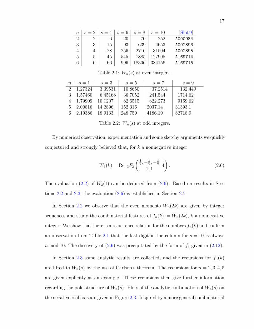
[Don09]. Some numerical values of Wn evaluated at integers are shown in Tables 2.1
and 2.2. One immediately notices the apparent integrality of the sequences for the
even moments—which are the moments of the squared expected distance, and where
the square root for s = 2 gives the root-mean-square distance√n. For n = 2, 3, 4 these
sequences were found in the Online Encyclopedia of Integer Sequences [Slo09]—the
cases n = 5, 6 are in the database as a consequence of this paper.
17
n s = 2 s = 4 s = 6 s = 8 s = 10 [Slo09]2 2 6 20 70 252 A000984
3 3 15 93 639 4653 A002893
4 4 28 256 2716 31504 A002895
5 5 45 545 7885 127905 A169714
6 6 66 996 18306 384156 A169715
Table 2.1: Wn(s) at even integers.
n s = 1 s = 3 s = 5 s = 7 s = 92 1.27324 3.39531 10.8650 37.2514 132.4493 1.57460 6.45168 36.7052 241.544 1714.624 1.79909 10.1207 82.6515 822.273 9169.625 2.00816 14.2896 152.316 2037.14 31393.16 2.19386 18.9133 248.759 4186.19 82718.9
Table 2.2: Wn(s) at odd integers.
By numerical observation, experimentation and some sketchy arguments we quickly
conjectured and strongly believed that, for k a nonnegative integer
W3(k) = Re 3F2
(12,−k
2,−k
2
1, 1
∣∣∣∣4) . (2.6)
The evaluation (2.2) of W3(1) can be deduced from (2.6). Based on results in Sec-
tions 2.2 and 2.3, the evaluation (2.6) is established in Section 2.5.
In Section 2.2 we observe that the even moments Wn(2k) are given by integer
sequences and study the combinatorial features of fn(k) := Wn(2k), k a nonnegative
integer. We show that there is a recurrence relation for the numbers fn(k) and confirm
an observation from Table 2.1 that the last digit in the column for s = 10 is always
n mod 10. The discovery of (2.6) was precipitated by the form of f3 given in (2.12).
In Section 2.3 some analytic results are collected, and the recursions for fn(k)
are lifted to Wn(s) by the use of Carlson’s theorem. The recursions for n = 2, 3, 4, 5
are given explicitly as an example. These recursions then give further information
regarding the pole structure of Wn(s). Plots of the analytic continuation of Wn(s) on
the negative real axis are given in Figure 2.3. Inspired by a more general combinatorial

18
convolution given in Section 2.2 we conjecture, for n = 1, 2, . . ., the recursion
W2n(s)?=∑j>0
(s/2
j
)2
W2n−1(s− 2j),
which has been partially resolved in [BSW11].
-6 -4 -2 2
-3
-2
-1
1
2
3
4
(a) W3
-6 -4 -2 2
-3
-2
-1
1
2
3
4
(b) W4
-6 -4 -2 2
-3
-2
-1
1
2
3
4
(c) W5
-6 -4 -2 2
-3
-2
-1
1
2
3
4
(d) W6
Figure 2.3: Various Wn and their analytic continuations.
2.2 The even moments and their combinatorial
features
In the case s = 2k the square root implicit in the definition (2.1) of Wn(s) dis-
appears, resulting in the fact that the even moments Wn(2k) are integers. In this
section we collect several of the combinatorial features of these moments which, while
sometimes in principle routine, provide important guidance and foundation. For in-
stance, the combinatorial expression for W3(2k) will eventually lead to the evaluation
of all integer moments W3(k) in Section 2.5. As a second example, the recurrence

19
equation, in its explicit form, for W4(2k) is at the heart of the derivation of the closed
form (2.5) in [BSWZ11].
In fact, the even moments are given as sums of squares of multinomials—as is
detailed next. While this result may be readily obtained from general probabilistic
principles starting with the observation that the characteristic function of the distance
traveled in n steps is given by the Bessel function Jn0 (see Section 2.4), we prefer to
give an elementary derivation starting from the integral definition (2.1) of Wn(s).
Proposition 2.2.1. For nonnegative integers k and n,
Wn(2k) =∑
a1+···+an=k
(k
a1, . . . , an
)2
.
Proof. In the spirit of the residue theorem of complex analysis, if f(x1, . . . , xn) has a
Laurent expansion around the origin then
ct f(x1, . . . , xn) =
∫[0,1]n
f(e2πix1 , . . . , e2πixn) dx, (2.7)
where ‘ct’ denotes the operator which extracts from an expression the constant term
of its Laurent expansion. In light of (2.7), the integral definition (2.1) of Wn(s) may
be restated as
Wn(s) = ct ((x1 + · · ·+ xn)(1/x1 + · · ·+ 1/xn))s/2 , (2.8)
see also Appendix 2.6.1. In the case s = 2k the right-hand side may be finitely
expanded to yield the claim: on using the multinomial theorem,
(x1+ · · ·+ xn)k (1/x1 + · · ·+ 1/xn)k
=∑
a1+···+an=k
(k
a1, . . . , an
)xa11 · · ·xann
∑b1+···+bn=k
(k
b1, . . . , bn
)x−b11 · · ·x−bnn ,

20
and the constant term is now obtained by matching a1 = b1, . . . , an = bn.
Remark 2.2.2. In the case that s is not an even integer, the right-hand side of (2.8)
may still be expanded, say, when Re s > 0 to obtain the series evaluation
Wn(s) = ns∑m>0
(−1)m(s/2
m
) m∑k=0
(−1)k
n2k
(m
k
) ∑a1+···+an=k
(k
a1, . . . , an
)2
. (2.9)
An alternative elementary proof of this expansion is given in Appendix 2.6.1. We
include this alternative proof, which chronologically was our first one, because, as a
side-product, it yields other interesting integral evaluations. ♦
In light of Proposition 2.2.1, we consider the combinatorial sums
fn(k) =∑
a1+···+an=k
(k
a1, . . . , an
)2
. (2.10)
of multinomial coefficients squared. These numbers also appear in [RS09] in the
following way: fn(k) counts the number of abelian squares of length 2k over an
alphabet with n letters (that is strings xx′ of length 2k from an alphabet with n
letters such that x′ is a permutation of x). It is not hard to see that
fn1+n2(k) =k∑j=0
(k
j
)2
fn1(j) fn2(k − j), (2.11)
for two non-overlapping alphabets with n1 and n2 letters. In particular, we may use
(2.11) to obtain f1(k) = 1, f2(k) =(
2kk
), as well as
f3(k) =k∑j=0
(k
j
)2(2j
j
)= 3F2
(12,−k,−k
1, 1
∣∣∣∣4) =
(2k
k
)3F2
(−k,−k,−k1,−k + 1
2
∣∣∣∣14),
(2.12)
f4(k) =k∑j=0
(k
j
)2(2j
j
)(2(k − j)k − j
)=
(2k
k
)4F3
( 12,−k,−k,−k1, 1,−k + 1
2
∣∣∣∣1) . (2.13)

21
Here and below pFq notates the generalised hypergeometric function. In general,
(2.11) can be used to write fn as a sum with at most dn/2e − 1 summation indices.
We recall a generating function for (fn(k))∞k=0 used in [BBBG08]. Let In(z) denote
the modified Bessel function of the first kind. Then
∑k>0
fn(k)zk
(k!)2=
(∑k>0
zk
(k!)2
)n
= 0F1(1; z)n = I0(2√z)n. (2.14)
It can be anticipated from (2.10) that, for fixed n, the sequence fn(k) will satisfy
a linear recurrence with polynomial coefficients. A procedure for constructing these
recurrences has been given in [Bar64]; in particular, that paper gives the recursions
for 3 6 n 6 6 explicitly. Moreover, an explicit general formula for the recurrences is
given in [Ver04]:
Theorem 2.2.3. For fixed n > 2, the sequence fn(k) satisfies a recurrence of order
λ = dn/2e with polynomial coefficients of degree n− 1:
∑j>0
kn−1∑
α1,...,αj
j∏i=1
−αi(n+ 1− αi)(
k − ik − i+ 1
)αi−1 fn(k − j) = 0. (2.15)
Here, the sum is over all sequences α1, . . . , αj such that 0 6 αi 6 n and αi+1 6 αi−2.
The recursions for n = 2, 3, 4, 5 are listed in Example 2.3.4 in Section 2.3.3, for-
mulated in terms of Wn(s) as per Theorem 2.3.3. As a consequence of Theorem 2.2.3
we obtain:
Theorem 2.2.4. For fixed n > 2, the sequence fn(k) satisfies a recurrence of order
λ = dn/2e with polynomial coefficients of degree n− 1:
cn,0(k)fn(k) + · · ·+ cn,λ(k)fn(k + λ) = 0 (2.16)

22
where
cn,0(k) = (−1)λ (n!!)2(k +
n
4
)n+1−2λλ−1∏j=1
(k + j)2 , (2.17)
and cn,λ(k) = (k + λ)n−1. Here n!! =∏λ−1
i=0 (n− 2i) is the double factorial.
Proof. The claim for cn,λ follows straight from (2.15). By (2.15), cn,0 is given by
cn,0(k − λ) =
[kn−1
∑α1,...,αλ
λ∏i=1
−αi(n+ 1− αi)(
k − ik − i+ 1
)αi−1]
(2.18)
where the sum is again over all sequences α1, . . . , αλ such that 0 6 αi 6 n and
αi+1 6 αi − 2.
If n is odd then there is only one such sequence, namely {n, n− 2, n− 4, . . .}, and
it follows that
cn,0(k − λ) = (−1)λ (n!!)2λ−1∏j=1
(k − j)2 (2.19)
in accordance with (2.17).
When n = 2λ is even, there are λ+1 sequences, namely α0 = {n, n−2, n−4, . . . , 2},
and αi for 1 6 i 6 λ, where αi is constructed from α0 by subtracting all elements by
1 starting from the (λ+ 1− i)th position.
Now by (2.18), we have
cn,0(k − λ) = (−1)λ
(λ−1∏i=1
(k − i)2
)λ∑j=0
(λ∏i=1
aji (n+ 1− aji ))
(k − λ+ j), (2.20)
where aji denotes the ith element of aj.
We make the key observation that the sum in (2.20) is symmetric, so writing it
backwards and adding that to itself, we factor out the term involving k:
2λ∑j=0
(λ∏i=1
aji (n+ 1− aji ))
(k − λ+ j) = (2k − λ)λ∑j=0
λ∏i=1
aji (n+ 1− aji ). (2.21)

23
As we know the sequences aj explicitly, the product on the right of (2.21) simplifies
to
(2λ)!
(2jj
)(2λ−2jλ−j
)(2λλ
) .
Hence the sum on the right of (2.21) is
λ∑j=0
(2λ)!
(2jj
)(2λ−2jλ−j
)(2λλ
) = 22λλ!2, (2.22)
which can be verified, for instance, using the snake oil method ([Wil90]). Substituting
this into (2.20) gives (2.17) for even n.
Remark 2.2.5. For fixed k, the map n 7→ fn(k) can be given by the evaluation of a
polynomial in n of degree k. This follows from
fn(k) =k∑j=0
(n
j
) ∑a1+···+aj=k
ai>0
(k
a1, . . . , aj
)2
, (2.23)
because the right-hand side is a linear combination (with positive coefficients only
depending on k) of the polynomials(nj
)= n(n−1)···(n−j+1)
j!in n of degree j for j =
0, 1, . . . , k.
From (2.23) the coefficient of(nk
)is seen to be (k!)2. We therefore formally obtain
the first-order approximation Wn(s) ≈n ns/2Γ(s/2 + 1) for n going to infinity, see also
[Klu06]. In particular, Wn(1) ≈n√nπ/2. Similarly, the coefficient of
(nk−1
)is k−1
4(k!)2
which gives rise to the second-order approximation
(k!)2
(n
k
)+k − 1
4(k!)2
(n
k − 1
)= k!nk − k(k − 1)
4k!nk−1 +O(nk−2)
of fn(k). We therefore obtain
Wn(s) ≈n ns/2−1
{(n− 1
2
)Γ(s
2+ 1)
+ Γ(s
2+ 2)− 1
4Γ(s
2+ 3)}
,

24
which is exact for s = 0, 2, 4. In particular, Wn(1) ≈n√nπ/2 +
√π/n/32. More
general approximations are given in [Cra09]. ♦
Remark 2.2.6. It follows straight from (2.10) that, for primes p, fn(p) ≡ n modulo
p. Further, for k > 1, fn(k) ≡ n modulo 2. This may be derived inductively from the
recurrence (2.11) since, assuming that fn(k) ≡ n modulo 2 for some n and all k > 1,
fn+1(k) =k∑j=0
(k
j
)2
fn(j) ≡ 1 +k∑j=1
(k
j
)n = 1 + n(2k − 1) ≡ n+ 1 (mod 2).
Hence for odd primes p,
fn(p) ≡ n (mod 2p). (2.24)
The congruence (2.24) also holds for p = 2 since fn(2) = (2n− 1)n, compare (2.23).
In particular, (2.24) confirms that indeed the last digit in the column for s = 10 is
always n mod 10—an observation from Table 2.1. ♦
Remark 2.2.7. The integers f3(k) (respectively f4(k)) also arise in physics, see for
instance [BBBG08], and are referred to as hexagonal (respectively diamond) lattice in-
tegers. The corresponding entries in Sloane’s online encyclopedia [Slo09] are A002893
and A002895. We recall the following formulae [BBBG08, (186)–(188)], relating these
sequences in non-obvious ways:
(∑k>0
f3(k)(−x)k
)2
=∑k>0
f2(k)3 x3k
((1 + x)3(1 + 9x))k+ 12
=∑k>0
f2(k)f3(k)(−x(1 + x)(1 + 9x))k
((1− 3x)(1 + 3x))2k+1
=∑k>0
f4(k)xk
((1 + x)(1 + 9x))k+1.

25
It would be instructive to similarly engage f5(k) for which we have
f5(k) =
(2 k
k
) k∑j=0
(kj
)4(2 k2 j
) 3F2
(−j,−j,−j1, 1
2− j
∣∣∣∣14),
as follows from (2.11). ♦
2.3 Analytic features of the moments
This section collects analytic features of the moments Wn(s) as a function in s. In
particular, it is shown that the recurrences for the even moments Wn(2k), described
in Section 2.2, extend to functional equations. This is deduced in the usual way from
Carlson’s theorem. Still we find it instructive to give the details, especially as the
explicit form of the functional equations and the resulting pole structures were crucial
for discovery and proof of the closed forms in the cases n = 3, 4, 5 obtained in here
and in [BSW11, BSWZ11], as was true for the results in Section 2.2.
2.3.1 Analyticity
We start with a preliminary investigation of the analyticity of Wn(s) for a given
n. This analyticity also follows from the general principle that the moment functions
of bounded random variables are always analytic in a strip of the complex plane
containing the right half-plane—but again we prefer to give a short direct proof.
Proposition 2.3.1. Wn(s) is analytic at least for Re s > 0.
Proof. Let s0 be a real number such that the integral in (2.1) converges for s = s0.
Then we claim that Wn(s) is analytic in s for Re s > s0. To this end, let s be such

26
that s0 < Re s 6 s0 + λ for some real λ > 0. For any real 0 6 a 6 n,
|as| = aRe s 6 nλas0 ,
and therefore
sups0<Re s6s0+λ
∫[0,1]n
∣∣∣∣∣∣∣∣∣ n∑k=1
e2πixk
∣∣∣∣s∣∣∣∣∣ dx 6 nλWn(s0) <∞.
This local boundedness implies, see for instance [Mat01], that Wn(s) as defined by
the integral in (2.1) is analytic in s for Re s > s0. Since the integral clearly converges
for s = 0, the claim follows.
This result will be extended in Theorem 2.3.5 and Corollary 2.3.6.
2.3.2 n = 1 and n = 2
It follows straight from the integral definition (2.1) that W1(s) = 1. In the case
n = 2, direct integration of (2.40) with n = 2 yields
W2(s) = 2s+1
∫ 1/2
0
cos(πt)sdt =
(s
s/2
), (2.25)
which may also be obtained using (2.9). In particular, W2(1) = 4/π. It may be worth
noting that neither Maple 14 nor Mathematica 7 can evaluate W2(1) if it is entered
naively in form of the defining (2.1) (or expanded as the square root of a sum of
squares), each returning the symbolic answer ‘0’.

27
2.3.3 Functional equations
We may lift the recursive structure of fn, defined in Section 2.2, to Wn to a fair
degree on appealing to Carlson’s theorem [Tit39, 5.81]. We recall that a function f
is of exponential type in a region if |f(z)| 6Mec|z| for some constants M and c.
Theorem 2.3.2 (Carlson). Let f be analytic in the right half-plane Re z > 0 and of
exponential type with the additional requirement that
|f(z)| 6Med|z|
for some d < π on the imaginary axis Re z = 0. If f(k) = 0 for k = 0, 1, 2, . . . then
f(z) = 0 identically.
Theorem 2.3.3. Given that fn(k) satisfies a recurrence
cn,0(k)fn(k) + · · ·+ cn,λ(k)fn(k + λ) = 0
with polynomial coefficients cn,j(k) (see Theorem 2.2.4) then Wn(s) satisfies the cor-
responding functional equation
cn,0(s/2)Wn(s) + · · ·+ cn,λ(s/2)Wn(s+ 2λ) = 0,
for Re s > 0.
Proof. Let
Un(s) := cn,0(s)Wn(2s) + · · ·+ cn,λ(s)Wn(2s+ 2λ).
Since fn(k) = Wn(2k) by Proposition 2.2.1, Un(s) vanishes at the nonnegative integers
by assumption. Consequently, Un(s) is zero throughout the right half-plane and we
are done—once we confirm that Theorem 2.3.2 applies. By Proposition 2.3.1, Wn(s)
28
is analytic for Re s > 0. Clearly, |Wn(s)| 6 nRe s. Thus
|Un(s)| 6(|cn,0(s)|+ |cn,1(s)|n2 + · · ·+ |cn,λ(s)|n2λ
)n2 Re s.
In particular, Un(s) is of exponential type. Further, Un(s) is polynomially bounded
on the imaginary axis Re s = 0. Thus Un satisfies the growth conditions of Theorem
2.3.2.
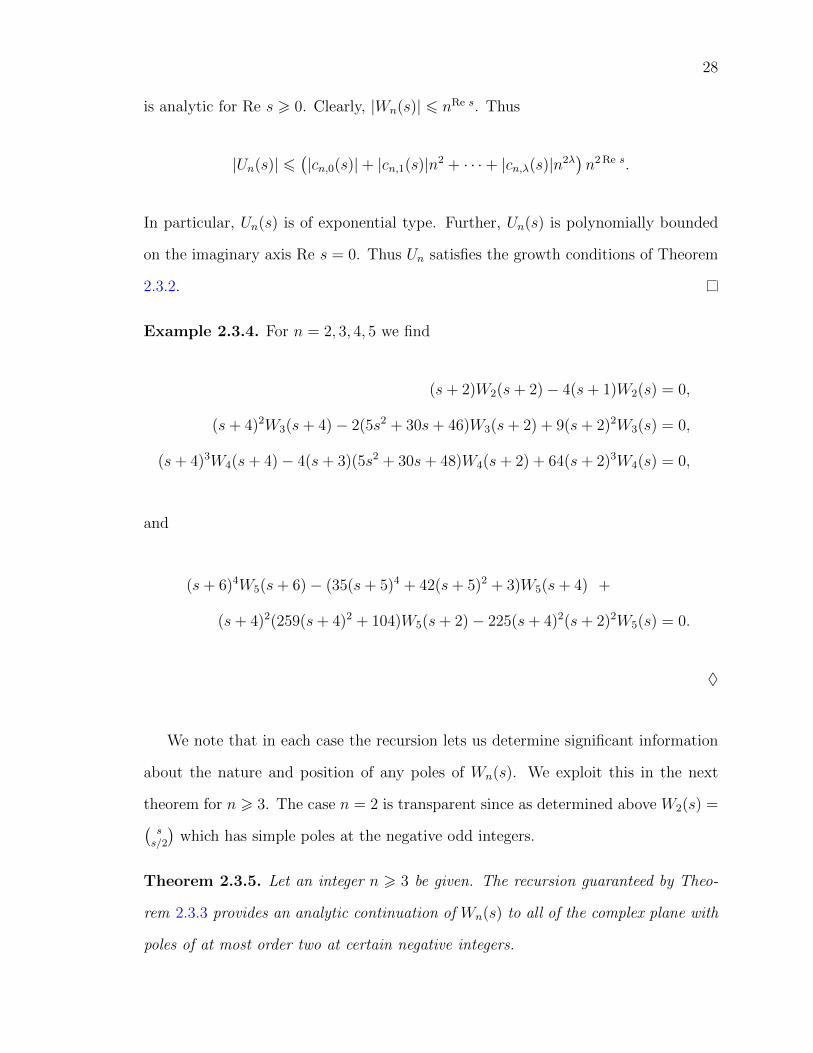
Example 2.3.4. For n = 2, 3, 4, 5 we find
(s+ 2)W2(s+ 2)− 4(s+ 1)W2(s) = 0,
(s+ 4)2W3(s+ 4)− 2(5s2 + 30s+ 46)W3(s+ 2) + 9(s+ 2)2W3(s) = 0,
(s+ 4)3W4(s+ 4)− 4(s+ 3)(5s2 + 30s+ 48)W4(s+ 2) + 64(s+ 2)3W4(s) = 0,
and
(s+ 6)4W5(s+ 6)− (35(s+ 5)4 + 42(s+ 5)2 + 3)W5(s+ 4) +
(s+ 4)2(259(s+ 4)2 + 104)W5(s+ 2)− 225(s+ 4)2(s+ 2)2W5(s) = 0.
♦
We note that in each case the recursion lets us determine significant information
about the nature and position of any poles of Wn(s). We exploit this in the next
theorem for n > 3. The case n = 2 is transparent since as determined above W2(s) =(ss/2
)which has simple poles at the negative odd integers.
Theorem 2.3.5. Let an integer n > 3 be given. The recursion guaranteed by Theo-
rem 2.3.3 provides an analytic continuation of Wn(s) to all of the complex plane with
poles of at most order two at certain negative integers.
29
Proof. Proposition 2.3.1 proves analyticity in the right halfplane. It is clear that
the recursion given by Theorem 2.3.3 ensures an analytic continuation with poles
only possible at negative integer values compatible with the recursion. Indeed, with
λ = dn/2e we have
Wn(s) = −cn,1(s/2)Wn(s+ 2) + · · ·+ cn,λ(s/2)Wn(s+ 2λ)
cn,0(s/2)(2.26)
with the cn,j as in (2.16). We observe that the right side of (2.26) only involves
Wn(s + 2k) for k > 1. Therefore the least negative pole can only occur at a zero of
cn,0(s/2) which is explicitly given in (2.17). We then note that the recursion forces
poles to be simple or of order two, and to be replicated as claimed.
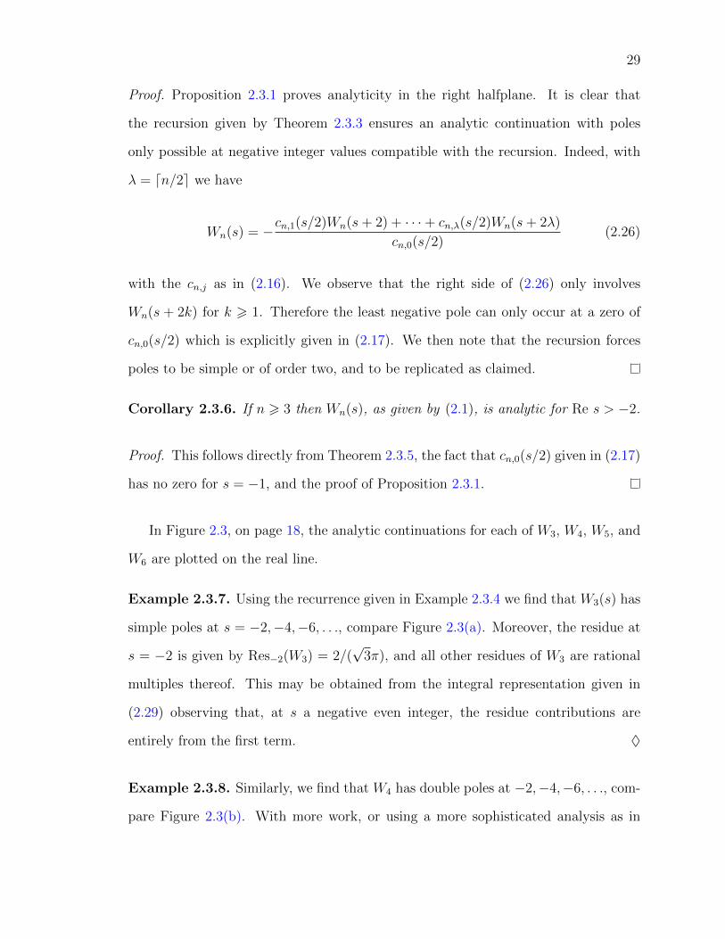
Corollary 2.3.6. If n > 3 then Wn(s), as given by (2.1), is analytic for Re s > −2.
Proof. This follows directly from Theorem 2.3.5, the fact that cn,0(s/2) given in (2.17)
has no zero for s = −1, and the proof of Proposition 2.3.1.
In Figure 2.3, on page 18, the analytic continuations for each of W3, W4, W5, and
W6 are plotted on the real line.
Example 2.3.7. Using the recurrence given in Example 2.3.4 we find that W3(s) has
simple poles at s = −2,−4,−6, . . ., compare Figure 2.3(a). Moreover, the residue at
s = −2 is given by Res−2(W3) = 2/(√
3π), and all other residues of W3 are rational
multiples thereof. This may be obtained from the integral representation given in
(2.29) observing that, at s a negative even integer, the residue contributions are
entirely from the first term. ♦
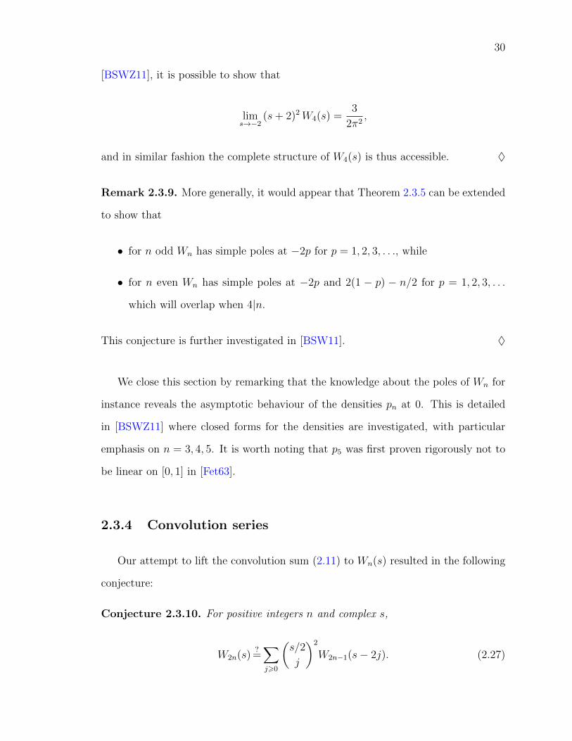
Example 2.3.8. Similarly, we find that W4 has double poles at −2,−4,−6, . . ., com-
pare Figure 2.3(b). With more work, or using a more sophisticated analysis as in
30
[BSWZ11], it is possible to show that
lims→−2
(s+ 2)2W4(s) =3
2π2,
and in similar fashion the complete structure of W4(s) is thus accessible. ♦
Remark 2.3.9. More generally, it would appear that Theorem 2.3.5 can be extended
to show that
• for n odd Wn has simple poles at −2p for p = 1, 2, 3, . . ., while
• for n even Wn has simple poles at −2p and 2(1 − p) − n/2 for p = 1, 2, 3, . . .
which will overlap when 4|n.
This conjecture is further investigated in [BSW11]. ♦
We close this section by remarking that the knowledge about the poles of Wn for
instance reveals the asymptotic behaviour of the densities pn at 0. This is detailed
in [BSWZ11] where closed forms for the densities are investigated, with particular
emphasis on n = 3, 4, 5. It is worth noting that p5 was first proven rigorously not to
be linear on [0, 1] in [Fet63].
2.3.4 Convolution series
Our attempt to lift the convolution sum (2.11) to Wn(s) resulted in the following
conjecture:
Conjecture 2.3.10. For positive integers n and complex s,
W2n(s)?=∑j>0
(s/2
j
)2
W2n−1(s− 2j). (2.27)

31
It is understood that the right-hand side of (2.27) refers to the analytic continu-
ation of Wn as guaranteed by Theorem 2.3.5. Conjecture 2.3.10, which is consistent
with the pole structure described in Remark 2.3.9, has been confirmed by David
Broadhurst [Bro09] using a Bessel integral representation for Wn, given in (2.28),
for n = 2, 3, 4, 5 and odd integers s < 50 to a precision of 50 digits. By (2.11) the
conjecture clearly holds for s an even positive integer. For n = 1 it is confirmed next.
Example 2.3.11. For n = 1 we obtain from (2.27) using W1(s) = 1,
W2(s) =∑j>0
(s/2
j
)2
=
(s
s/2
)
which agrees with (2.25). ♦
We remark that a partial resolution of Conjecture 2.3.10 is obtained in [BSWZ11].
2.4 Bessel integral representations
As noted in the introduction, Kluyver [Klu06] made a lovely analysis of the cu-
mulative distribution function of the distance traveled by a “rambler” in the plane
for various fixed step lengths. In particular, for our uniform walk Kluyver provides
the Bessel function representation
Pn(t) = t
∫ ∞0
J1(xt) Jn0 (x) dx.
Thus, Wn(s) =∫ n
0ts pn(t) dt, where pn = P ′n. From here, Broadhurst [Bro09] obtains
Wn(s) = 2s+1−k Γ(1 + s2)
Γ(k − s2)
∫ ∞0
x2k−s−1
(−1
x
d
dx
)kJn0 (x) dx (2.28)
for real s and is valid as long as 2k > s > max(−2,−n2).

32
Remark 2.4.1. For n = 3, 4, symbolic integration in Mathematica of (2.28) leads to
interesting analytic continuations [Cra09] such as
W3(s) =1
22s+1tan(πs
2
)( ss−1
2
)2
3F2
( 12, 1
2, 1
2s+3
2, s+3
2
∣∣∣∣14)
+
(ss2
)3F2
(− s2,− s
2,− s
2
1,− s−12
∣∣∣∣14),
(2.29)
and
W4(s) =1
22stan(πs
2
)( ss−1
2
)3
4F3
( 12, 1
2, 1
2, s
2+ 1
s+32, s+3
2, s+3
2
∣∣∣∣1)+
(ss2
)4F3
( 12,− s
2,− s
2,− s
2
1, 1,− s−12
∣∣∣∣1) .(2.30)
We note that for s = 2k = 0, 2, 4, . . . the first term in (2.29) (resp. (2.30)) is
zero and the second is a formula given in (2.12) (resp. (2.13)). Thence, one can in
principle prove (2.29) and (2.30) by applying Carlson’s theorem—after showing the
singularities at 1, 3, 5, . . . are removable. A rigorous proof, along with extensions and
more details, appears in [BSW11]. ♦
2.5 The odd moments of a three-step walk
In this section, we combine the results of the previous sections to finally prove the
hypergeometric evaluation (2.6) of the moments W3(k) in Theorem 2.5.1.
It is elementary to express the distance y of an (n + 1)-step walk conditioned on
a given distance x of an n-step walk. By a simple application of the cosine rule we
find
y2 = x2 + 1 + 2x cos(θ),

33
where θ is the outside angle of the triangle with sides of lengths x, 1, and y:
\θx
yjjjjjjjjjjjjj
jjjjjjjjjjjjj 1�����
�����
It follows that the s-th moment of an (n+1)-step walk conditioned on a given distance
x of an n-step walk is
gs(x) :=1
π
∫ π
0
ys dθ = |x− 1|s 2F1
(12,− s
2
1
∣∣∣∣− 4x
(x− 1)2
). (2.31)
Here we appealed to symmetry to restrict the angle to θ ∈ [0, π). We then evaluated
the integral in hypergeometric form which, for instance, can be done with the help of
Mathematica. Observe that gs(x) does not depend on n. Since Wn+1(s) is the s-th
moment of the distance of an (n+ 1)-step walk, we obtain
Wn+1(s) =
∫ n
0
gs(x) pn(x) dx, (2.32)
where pn(x) is the density of the distance x for an n-step walk. Clearly, for the 1-step
walk we have p1(x) = δ1(x), a Dirac delta function at x = 1. It is also easily shown
that the probability density for a 2-step walk is given by p2(x) = 2(π√
4− x2)−1 for
0 6 x 6 2 and 0 otherwise. The density p3(x) is given in (2.3).
For n = 3, based on (2.12) we define
V3(s) := 3F2
(12,− s
2,− s
2
1, 1
∣∣∣∣4) , (2.33)
so that by Proposition 2.2.1 and (2.12), W3(2k) = V3(2k) for nonnegative integers
k. This led us to explore V3(s) more generally numerically and so to conjecture and
eventually prove the following:

34
Theorem 2.5.1. For nonnegative even integers and all odd integers k:
W3(k) = Re V3(k).
Remark 2.5.2. Note that, for all complex s, the function V3(s) also satisfies the
recursion given in Example 2.3.4 for W3(s)—as is routine to prove symbolically using
for instance creative telescoping [PWZ96]. However, V3 does not satisfy the growth
conditions of Carlson’s Theorem (Theorem 2.3.2). Thus, it yields a rather nice illus-
tration that the hypotheses can fail. ♦
Proof of Theorem 2.5.1. It remains to prove the result for odd integers. Since, as
noted in Remark 2.5.2, for all complex s, the function V3(s) defined in (2.33) also
satisfies the recursion given in Example 2.3.4, it suffices to show that the values given
for s = 1 and s = −1 are correct. From (2.32), we have the following expression for
W3:
W3(s) =2
π
∫ 2
0
gs(x)√4− x2
dx =2
π
∫ π/2
0
gs(2 sin(t))dt. (2.34)
For s = 1: equation (2.31), [BB98, Exercise 1c, p. 16], and Jacobi’s imaginary
transformations [BB98, Exercises 7a) & 8b), p. 73] allow us to write
π
2g1(x) = (x+ 1)E
(2√x
x+ 1
)= Re
(2E(x)− (1− x2)K(x)
)(2.35)

35
where K(k) =∫ π/2
0dt/√
1− k2 sin2(t) and E(k) =∫ π/2
0
√1− k2 sin2(t) dt denote the
complete elliptic integrals of the first and second kind. Thus, from (2.34) and (2.35),
W3(1) =4
π2Re
∫ π/2
0
(2E(2 sin(t))− (1− 4 sin2(t))K(2 sin(t))
)dt
=4
π2Re
∫ π/2
0
∫ π/2
0
2√
1− 4 sin2(t) sin2(r) dtdr
− 4
π2Re
∫ π/2
0
∫ π/2
0
1− 4 sin2(t)√1− 4 sin2(t) sin2(r)
dtdr.
Amalgamating the two last integrals and parameterizing, we consider
Q(a) :=4
π2
∫ π/2
0
∫ π/2
0
1 + a2 sin2(t)− 2 a2 sin2(t) sin2(r)√1− a2 sin2(t) sin2(r)
dtdr. (2.36)
We now use the binomial theorem to integrate (2.36) term-by-term for |a| < 1
and substitute 2π
∫ π/20
sin2m(t) dt = (−1)m(−1/2
m
)throughout. Moreover, (−1)m
(−αm
)=
(α)m/m! where the later denotes the Pochhammer symbol. Evaluation of the conse-
quent infinite sum produces:
Q(a) =∑k>0
(−1)k(−1/2
k
)(a2k
(−1/2
k
)2
− a2k+2
(−1/2
k
)(−1/2
k + 1
)− 2a2k+2
(−1/2
k + 1
)2)
=∑k>0
(−1)ka2k
(−1/2
k
)31
(1− 2k)2
= 3F2
(−12,−1
2, 1
2
1, 1
∣∣∣∣a2
).
Analytic continuation to a = 2 yields the claimed result as per for s = 1.

36
For s = −1: we similarly and more easily use (2.31) and (2.34) to derive
W3(−1) = Re4
π2
∫ π/2
0
K(2 sin(t)) dt
= Re4
π2
∫ π/2
0
∫ π/2
0
1√1− 4 sin2(t) sin2(r)
dtdr = V3(−1).
Example 2.5.3. Theorem 2.5.1 allows us to establish the following equivalent ex-
pressions for W3(1):
W3(1) =4√
3
3
(3F2
(−12,−1
2,−1
2
1, 1
∣∣∣∣14)− 1
π
)+
√3
243F2
(12, 1
2, 1
2
2, 2
∣∣∣∣14)
= 2√
3K2 (k3)
π2+√
31
K2 (k3)
=3
16
21/3
π4Γ6
(1
3
)+
27
4
22/3
π4Γ6
(2
3
).
These rely on using Legendre’s identity and several Clausen-like product formulae,
plus Legendre’s evaluation of K(k3) where k3 :=√
3−12√
2is the third singular value as
in [BB98]. More simply but similarly, we have
W3(−1) = 2√
3K2 (k3)
π2=
3
16
21/3
π4Γ6
(1
3
).
Using the recurrence presented in Example 2.3.4 it follows that similar expressions
can be given for W3 evaluated at odd integers.
In [BSW11], corresponding hypergeometric closed forms for W4 are presented. ♦

37
2.6 Appendix
2.6.1 An alternative proof of the series evaluation (2.9)
We begin with:
Proposition 2.6.1. For complex s with Re s > 0,
Wn(s) = ns∑m>0
(−1)m(s/2
m
)(2
n
)2m ∫[0,1]n
( ∑16i<j6n
sin2(π(xj − xi)))m
dx. (2.37)
Proof. Start with
∣∣∣∣∣n∑k=1
e2πixk
∣∣∣∣∣2
=
(n∑k=1
cos(2πxk)
)2
+
(n∑k=1
sin(2πxk)
)2
=
(∑i<j
(cos(2πxi) + cos(2πxj)
)2
+(
sin(2πxi) + sin(2πxj))2)− n(n− 2)
= 4
(∑i<j
cos2(π(xj − xi)))− n(n− 2)
= n2 − 4
(∑i<j
sin2(π(xj − xi))).
Therefore, noting that binomial expansion may be applied to the integrand outside a
set of n-dimensional measure zero,
Wn(s) =
∫[0,1]n
(n2 − 4
(∑i<j
sin2(π(xj − xi))))s/2
dx
= ns∫
[0,1]n
∑m>0
(−1)m(s/2
m
)(2
n
)2m(∑
i<j
sin2(π(xj − xi)))m
dx.
Thus the result follows once changing the order of integration and summation is
justified. Observe that if s is real then (−1)m(s/2m
)has a fixed sign for m > s/2 and
we can apply monotone convergence. On the other hand, if s is complex then we may

38
use
limm→∞
∣∣∣∣∣(s/2m
)(Re s/2m
)∣∣∣∣∣ =
∣∣∣∣Γ(−Re s/2)
Γ(−s/2)
∣∣∣∣ ,which follows from Stirling’s approximation, and apply dominated convergence using
the real case for comparison.
We next evaluate the integrals in (2.37):
Theorem 2.6.2. For nonnegative integers m,
∫[0,1]n
(∑i<j
sin2(π(xj − xi)))m
dx =(n
2
)2mm∑k=0
(−1)k
n2k
(m
k
) ∑a1+···+an=k
(k
a1, . . . , an
)2
.
Proof. Denote the left-hand by In,m. As in the proof of Proposition 2.2.1 we note
that the claim is equivalent to asserting that 22mIn,m is the constant term of
(n2 − (x1 + · · ·+ xn)(1/x1 + · · ·+ 1/xn))m.
Observe that
(n2 − (x1 + · · ·+ xn)(1/x1 + · · ·+ 1/xn))m =
( ∑16i<j6n
(2− xi
xj− xjxi
))m
= (−1)m
( ∑16i<j6n
(xj − xi)2
xixj
)m
.
The result therefore follows from the next proposition.
As before, we denote by ‘ct’ the operator which extracts from an expression the
constant term of its Laurent expansion.
Proposition 2.6.3. For any integers 1 6 i1 6= j1, . . . , im 6= jm 6 n,
∫[0,1]n
m∏k=1
4 sin2(π(xjk − xik)) dx = (−1)m ctm∏k=1
(xjk − xik)2
xikxjk.
39
Proof. We prove this by evaluating both sides independently. First, we have
LHS :=
∫[0,1]n
m∏k=1
4 sin2(π(xjk − xik)) dx
= (−1)m∫
[0,1]n
m∏k=1
(eπi(xjk−xik ) − e−πi(xjk−xik )
)2dx
= (−1)m∑a,b
(−1)∑k(ak+bk−2)/2
∫[0,1]n
eπi∑k(ak+bk)(xjk−xik ) dx
=∑a,b
(−1)∑k(ak+bk)/2
∫[0,1]n
cos
(π∑k
(ak + bk)(xjk − xik))
dx
where the last two sums are over all sequences a, b ∈ {±1}m. In the last step the
summands corresponding to (a, b) and (−a,−b) have been combined.
Now note that, for a an even integer,
∫ 1
0
cos(π(ax+ b))dx =
cos(πb) if a = 0,
0 otherwise.(2.38)
Since ak + bk is even, we may apply (2.38) iteratively to obtain
∫[0,1]n
cos
(π∑k
(ak + bk)(xjk − xik))
dx =
1 if a, b ∈ S,
0 otherwise,
where S denotes the set of sequences a, b ∈ {±1}m such that
m∑k=1
(ak + bk)(xjk − xik) = 0
as a polynomial in x. It follows that
LHS =∑a,b∈S
(−1)∑k(ak+bk)/2 (2.39)
40
On the other hand, consider
RHS := (−1)m ctm∏k=1
(xjk − xik)2
xikxjk,
and observe that, by a similar argument as above,
(−1)mm∏k=1
(xjk − xik)2
xikxjk=∑a,b
m∏k=1
(−1)(ak+bk)/2
(xjkxik
)(ak+bk)/2
where the sum is again over all sequences a, b ∈ {±1}m. From here, it is straight-
forward to verify that RHS is equivalent to the expression given for LHS in (2.39).
The desired evaluation is now available. On combining Theorem 2.6.2 and Propo-
sition 2.6.1 we obtain that for Re s > 0,
Wn(s) = ns∑m>0
(−1)m(s/2
m
) m∑k=0
(−1)k
n2k
(m
k
) ∑a1+···+an=k
(k
a1, . . . , an
)2
.
This is (2.9).
Remark 2.6.4. We briefly outline the experimental genesis of the evaluation given
in Proposition 2.2.1. The sequence 22mI3,m appearing in the proof of Theorem 2.6.2
is Sloane’s, [Slo09], A093388 where a link to [Ver99] is given. That paper contains
the sum
22mI3,m = (−1)mm∑k=0
(m
k
)(−8)k
m−k∑j=0
(m− kj
)3
and further mentions that 22mI3,m is therefore the coefficient of (xyz)m in
(8xyz − (x+ y)(y + z)(z + x))m.

41
Observe also that 22mI2,m is the coefficient of (xy)m in
(4xy − (x+ y)(y + x))m.
It was then noted that
8xyz − (x+ y)(y + z)(z + x) = 32xyz − (x+ y + z)(xy + yz + zx)
and this line of extrapolation led to the correct conjecture, so that the next case
would involve
42wxyz − (w + x+ y + z)(wxy + xyz + yzw + zwx),
which was what we have now proven. ♦
2.6.2 Numerical evaluations
A one-dimensional reduction of the integral (2.1) may be achieved by taking pe-
riodicity into account:
Wn(s) =
∫[0,1]n−1
∣∣∣∣∣1 +n−1∑k=1
e2πixk
∣∣∣∣∣s
d(x1, . . . , xn−1). (2.40)
From here, we note that quick and rough estimates are easily obtained using the
Monte Carlo method. Moreover, since the integrand function is periodic this seems
like an invitation to use lattice sequences—a quasi-Monte Carlo method. E.g., the
lattice sequence from [CKN06] can be straightforwardly employed to calculate an
entire table in one run by keeping a running sum over different values of n and s. A
standard stochastic error estimator can then be obtained by random shifting.

42
Generally, however, Broadhurst’s representation (2.28) seems to be the best avail-
able for high precision evaluations of Wn(s). We close by commenting on the special
cases n = 3, 4.
Example 2.6.5. The first high precision evaluations of W3 were performed by David
Bailey who confirmed the initially only conjectured Theorem 2.5.1 for s = 2, . . . , 7
to 175 digits. This was done on a 256-core LBNL system in roughly 15 minutes by
applying tanh-sinh integration to
W3(s) =
∫ 1
0
∫ 1
0
(9− 4(sin2(πx) + sin2(πy) + sin2(π(x− y)))
)s/2dydx,
which is obtained from (2.40) as in Proposition 2.6.1. More practical is the one-
dimensional form (2.34) which can deliver high precision results in minutes on a simple
laptop. For integral s, Theorem 2.5.1 allows extremely high precision evaluations. ♦
Example 2.6.6. Assuming that Conjecture 2.3.10 holds for n = 2 (for a proof, see
[BSWZ11]), Theorem 2.5.1 implies that for nonnegative integers k
W4(k)?= Re
∑j>0
(s/2
j
)2
3F2
(12,−k
2+ j,−k
2+ j
1, 1
∣∣∣∣4) .This representation is very suitable for high precision evaluations of W4 since, roughly,
one correct digit is added by each term of the sum. Formula (2.30) by Crandall also
lends itself quite well for numerical work (by slightly perturbing even s for integer
arguments). ♦

43
Chapter 3
Three-step and four-step randomwalk integrals
The contents of this chapter (apart from minor corrections or adaptions) have
been published as:
[BSW11] Three-step and four-step random walk integrals(with Jonathan M. Borwein, James Wan)
to appear in Experimental Mathematics
Abstract We investigate the moments of 3-step and 4-step uniform random walks
in the plane. In particular, we further analyse a formula conjectured in [BNSW11]
expressing 4-step moments in terms of 3-step moments. Diverse related results in-
cluding hypergeometric and elliptic closed forms for W4(±1) are given and two new
conjectures are recorded.
3.1 Introduction and preliminaries
Continuing research commenced in [BNSW11], for complex s, we consider the
n-dimensional integral
Wn(s) :=
∫[0,1]n
∣∣∣∣∣n∑k=1
e2πxki
∣∣∣∣∣s
dx (3.1)
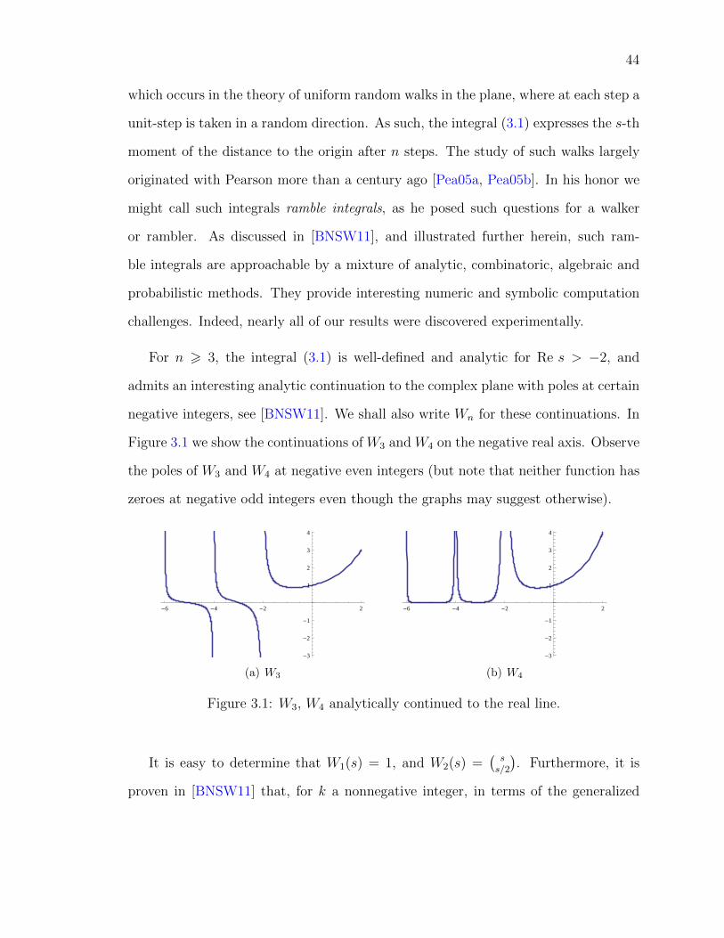
44
which occurs in the theory of uniform random walks in the plane, where at each step a
unit-step is taken in a random direction. As such, the integral (3.1) expresses the s-th
moment of the distance to the origin after n steps. The study of such walks largely
originated with Pearson more than a century ago [Pea05a, Pea05b]. In his honor we
might call such integrals ramble integrals, as he posed such questions for a walker
or rambler. As discussed in [BNSW11], and illustrated further herein, such ram-
ble integrals are approachable by a mixture of analytic, combinatoric, algebraic and
probabilistic methods. They provide interesting numeric and symbolic computation
challenges. Indeed, nearly all of our results were discovered experimentally.
For n > 3, the integral (3.1) is well-defined and analytic for Re s > −2, and
admits an interesting analytic continuation to the complex plane with poles at certain
negative integers, see [BNSW11]. We shall also write Wn for these continuations. In
Figure 3.1 we show the continuations of W3 and W4 on the negative real axis. Observe
the poles of W3 and W4 at negative even integers (but note that neither function has
zeroes at negative odd integers even though the graphs may suggest otherwise).
-6 -4 -2 2
-3
-2
-1
1
2
3
4
(a) W3
-6 -4 -2 2
-3
-2
-1
1
2
3
4
(b) W4
Figure 3.1: W3, W4 analytically continued to the real line.
It is easy to determine that W1(s) = 1, and W2(s) =(ss/2
). Furthermore, it is
proven in [BNSW11] that, for k a nonnegative integer, in terms of the generalized

45
hypergeometric function, we have
W3(k) = Re 3F2
(12,−k
2,−k
2
1, 1
∣∣∣∣4) . (3.2)
From here, the following expressions for W3(1) can be established:
W3(1) =4√
3
3
(3F2
(−12,−1
2,−1
2
1, 1
∣∣∣∣14)− 1
π
)+
√3
243F2
(12, 1
2, 1
2
2, 2
∣∣∣∣14)
(3.3)
= 2√
3K2 (k3)
π2+√
31
K2 (k3)(3.4)
=3
16
21/3
π4Γ6
(1
3
)+
27
4
22/3
π4Γ6
(2
3
)(3.5)
=1
π2
(21/3
4β2
(1
3
)+ 22/3β2
(2
3
)), (3.6)
where K is the complete elliptic integral of the first kind, k3 :=√
3−12√
2is the third
singular value as in [BB98], and β(x) := B(x, x) is a central Beta-function value.
More simply, but similarly,
W3(−1) = 2√
3K2 (k3)
π2=
3
16
21/3
π4Γ6
(1
3
)=
213
4π2β2
(1
3
). (3.7)
Using the two-term recurrence for W3 given in [BNSW11], it follows that similar
expressions can be given for W3 evaluated at any odd integer. It is one of the goals
of this paper to give similar evaluations for a 4-step walk.
For s an even positive integer, the moments Wn(s) take explicit integer values. In
fact, for integers k > 0,
Wn(2k) =∑
a1+···+an=k
(k
a1, . . . , an
)2
. (3.8)
Based on the combinatorial properties of this evaluation, the following conjecture was
made in [BNSW11]. Note that the case n = 1 is easily resolved.
46
Conjecture 3.1.1. For positive integers n and complex s,
W2n(s)?[1]=∑j>0
(s/2
j
)2
W2n−1(s− 2j). (3.9)
We investigate this conjecture in some detail in Section 3.4. For n = 2, in conjunc-
tion with (3.3) this leads to a very efficient computation of W4 at integers, yielding
roughly a digit per term.
3.2 Bessel integral representations
We start with the result of Kluyver [Klu06], amplified in [Wat41, §31.48] and
exploited in [BNSW11], to the effect that the probability that an n-step walk ends
up within a disc of radius α is
Pn(α) = α
∫ ∞0
J1(αx)Jn0 (x) dx. (3.10)
From this, David Broadhurst [Bro09] obtains
Wn(s) = 2s+1−k Γ(1 + s2)
Γ(k − s2)
∫ ∞0
x2k−s−1
(−1
x
d
dx
)kJn0 (x) dx (3.11)
valid as long as 2k > s > −n/2. Here and below Jν(z) denotes the Bessel function
of the first kind.
Example 3.2.1 (Wn(±1)). In particular, from (3.11), for n > 2, we can write:
Wn(−1) =
∫ ∞0
Jn0 (x) dx, Wn(1) = n
∫ ∞0
J1(x)J0(x)n−1 dx
x. (3.12)
♦

47
Equation (3.11) enabled Broadhurst to verify Conjecture 3.1.1 for n = 2, 3, 4, 5
and odd positive s < 50 to a precision of 50 digits. A different proof of (3.11) is
outlined in Remark 3.2.3 below. In particular, for 0 < s < n/2, we have
Wn(−s) = 21−sΓ(1− s/2)
Γ(s/2)
∫ ∞0
xs−1Jn0 (x) dx, (3.13)
so that Wn(−s) essentially is (the analytic continuation of) the Mellin transform of
the nth power of the Bessel function J0.
Example 3.2.2. Using (3.13), the evaluations W1(s) = 1 and W2(s) =(ss/2
)translate
into
∫ ∞0
xs−1J0(x) dx = 2s−1 Γ(s/2)
Γ(1− s/2),∫ ∞
0
xs−1J20 (x) dx =
1
2Γ(1/2)
Γ(s/2)Γ(1/2− s/2)
Γ(1− s/2)2
in the region where the left-hand side converges.
The Mellin transforms of J30 and J4
0 in terms of Meijer G-functions appear in the
proofs of Theorems 3.2.7 and 3.2.8. ♦
Remark 3.2.3. Here, we demonstrate how Ramanujan’s “master theorem” may be
applied to find the Bessel integral representation (3.11) in a natural way; this and
more applications of Ramanujan’s master theorem will appear in [AEG+11]. For an
alternative proof see [Bro09].
Ramanujan’s master theorem [Har78] states that, under certain conditions on the
analytic function ϕ,
∫ ∞0
xν−1
(∞∑k=0
(−1)k
k!ϕ(k)xk
)= Γ(ν)ϕ(−ν). (3.14)
48
Based on the evaluation (3.8), we have, as noted in [BNSW11], the generating
function ∑k>0
Wn(2k)(−x)k
(k!)2=
(∑k>0
(−x)k
(k!)2
)n
= J0(2√x)n (3.15)
for the even moments. Applying Ramanujan’s master theorem (3.14) to ϕ(k) :=
Wn(2k)/k!, we find
Γ(ν)ϕ(−ν) =
∫ ∞0
xν−1Jn0 (2√x) dx. (3.16)
Upon a change of variables and setting s = 2ν,
Wn(−s) = 21−sΓ(1− s/2)
Γ(s/2)
∫ ∞0
xs−1Jn0 (x) dx. (3.17)
This is the case k = 0 of (3.11). The general case follows from the fact that if F (s)
is the Mellin transform of f(x), then (s− 2)(s− 4) · · · (s− 2k)F (s− 2k) is the Mellin
transform of(− 1x
ddx
)kf(x). ♦
3.2.1 Pole structure
A very useful consequence of equation (3.13) is the following proposition.
Proposition 3.2.4 (Poles). The structure of the poles of Wn is as follows:
(a) (Reflection) For n = 3, we have explicitly for k = 0, 1, 2, . . . that
Res(−2k−2)(W3) =2
π√
3
W3(2k)
32k> 0,
and the corresponding poles are simple.

49
(b) For each integer n > 5, the function Wn(s) has a simple pole at −2k − 2 for
integers 0 6 k < (n− 1)/4 with residue given by
Res(−2k−2)(Wn) =(−1)k
22k(k!)2
∫ ∞0
x2k+1Jn0 (x) dx. (3.18)
(c) Moreover, for odd n > 5, all poles of Wn(s) are simple as soon as the first (n−1)/2
are.
In fact, we believe that for odd n, all poles of Wn(s) are simple as stated in
Conjecture 3.4.1. For individual n this may be verified as in Example 3.2.5. This was
done by the authors for n 6 45.
Proof. (a) For n = 3 it was shown in [BNSW11] that Res−2(W3) = 2/(√
3π). This
also follows from (3.24) of Corollary 3.2.9. We remark that from [Wat41, (4)
p. 412] this is also the value of the conditional integral∫∞
0xJ3
0 (x) dx in accordance
with (3.18). Letting r3(k) := Res(−2k)(Wn), the explicit residue equation is
r3 (k) =(10 k2 − 30 k + 23) r3(k − 1)− (k − 2)2r3(k − 2)
9 (k − 1)2,
which has the asserted solution, when compared to the recursion for W3(s):
(s+ 4)2W3(s+ 4)− 2(5s2 + 30s+ 46)W3(s+ 2) + 9(s+ 2)2W3(s) = 0. (3.19)
We give another derivation in Example 3.3.4 in Section 3.3.
(b) For n > 5 we note that the integral in (3.18) is absolutely convergent since
|J0(x)| 6 1 on the real axis and J0(x) ≈√
2/(πx) cos(x − π/4) (see [AS72,
(9.2.1)]). Since
lims→2k
(s− 2k)Γ(1− s/2) = 2(−1)k
(k − 1)!,

50
the residue is as claimed by (3.17).
(c) As shown in [BNSW11] Wn, for odd n, satisfies a recursion of the form
(−1)λ (n!!)2λ−1∏j=1
(s+ 2j)2 Wn(s)+c1(s)Wn(s+2)+· · ·+(s+ 2λ)n−1Wn(s+2λ) = 0,
with polynomial coefficients of degree n− 1 where λ := (n+ 1)/2. From this, on
multiplying by (s+2k)(s+2k−2) · · · (s−2k+2λ) one may derive a corresponding
recursion for Res(−2k)(Wn) for k = 1, 2, . . . Inductively, this lets us establish that
the poles are simple. The argument breaks down if one of the initial values is
infinite as it is when 4|n.
Example 3.2.5 (Poles of W5). We illustrate Proposition 3.2.4 in the case n = 5. In
particular, we demonstrate how to show that all poles are indeed simple. To this end,
we start with the recursion:
(s+ 6)4W5(s+ 6)− (35(s+ 5)4 + 42(s+ 5)2 + 3)W5(s+ 4)
+ (s+ 4)2(259(s+ 4)2 + 104)W5(s+ 2) = 225(s+ 4)2(s+ 2)2W5(s).
From here,
lims→−2
(s+ 2)2W5(s) =4
225(285W5(0)− 201W5(2) + 16W5(4)) = 0
which shows that the first pole is indeed simple as is also guaranteed by Proposition
3.2.4b. Similarly,
lims→−4
(s+ 4)2W5(s) = − 4
225(5W5(0)−W5(2)) = 0
51
showing that the second pole is simple as well. It follows from Proposition 3.2.4c that
all poles of W5 are simple. More specifically, let r5(k) := Res(−2k)(W5). With initial
values r5(0) = 0, r5(1) and r5(2), we derive that
r5(k + 3) =k4r5(k)− (5 + 28 k + 63 k2 + 70 k3 + 35 k4) r5(k + 1)
225(k + 1)2(k + 2)2
+(285 + 518 k + 259 k2) r5(k + 2)
225(k + 2)2.
♦
3.2.2 Meijer G-function representations
The Meijer G-function was introduced in 1936 by the Dutch mathematician Cor-
nelis Simon Meijer (1904-1974). It is defined, for parameter vectors a and b [AAR99],
by
Gm,np,q
(a
b
∣∣∣∣x) = Gm,np,q
(a1, . . . , apb1, . . . , bq
∣∣∣∣x)=
1
2πi
∫L
∏mk=1 Γ(bk − t)
∏nk=1 Γ(1− ak + t)∏q
k=m+1 Γ(1− bk + t)∏p
k=n+1 Γ(ak − t)xt dt. (3.20)
In the case |x| < 1 and p = q the contour L is a loop that starts at infinity on a
line parallel to the positive real axis, encircles the poles of the Γ(bk − t) once in the
negative sense and returns to infinity on another line parallel to the positive real axis.
L is a similar contour when |x| > 1. Moreover Gp,qm,n is analytic in each parameter; in
consequence so are the compositions arising below.
Our main tool below is the following special case of Parseval’s formula giving the
Mellin transform of a product.

52
Theorem 3.2.6. Let G(s) and H(s) be the Mellin transforms of g(x) and h(x) re-
spectively. Then
∫ ∞0
xs−1g(x)h(x) dx =1
2πi
∫ δ+i∞
δ−i∞G(z)H(s− z) dz (3.21)
for any real number δ in the common region of analyticity.
This leads to:
Theorem 3.2.7 (Meijer form for W3). For all complex s
W3(s) =Γ(1 + s/2)
Γ(1/2)Γ(−s/2)G2,1
3,3
(1, 1, 1
1/2,−s/2,−s/2
∣∣∣∣14). (3.22)
Proof. We apply Theorem 3.2.6 to J30 = J2
0 · J0 for s in a vertical strip. Using
Example 3.2.2 we then obtain
∫ ∞0
xs−1J30 (x) dx =
1
2πi
∫ δ+i∞
δ−i∞
2s−z−2
Γ(1/2)
Γ(z/2)Γ(1/2− z/2)
Γ(1− z/2)2
Γ(s/2− z/2)
Γ(1− s/2 + z/2)dz
=2s
2Γ(1/2)
1
2πi
∫ δ/2+i∞
δ/2−i∞4−t
Γ(t)Γ(1/2− t)Γ(s/2− t)Γ(1− t)2Γ(1− s/2 + t)
dt
=2s
2Γ(1/2)G2,1
3,3
(1, 1, 1
1/2, s/2, s/2
∣∣∣∣14)
where 0 < δ < 1. The claim follows from (3.17) by analytic continuation.
Similarly we obtain:
Theorem 3.2.8 (Meijer form for W4). For all complex s with Re s > −2
W4(s) =2s
π
Γ(1 + s/2)
Γ(−s/2)G2,2
4,4
(1, (1− s)/2, 1, 1
1/2,−s/2,−s/2,−s/2
∣∣∣∣1) . (3.23)

53
Proof. We now apply Theorem 3.2.6 to J40 = J2
0 · J20 , again for s in a vertical strip.
Using once more Example 3.2.2, we obtain
∫ ∞0
xs−1J40 (x) dx =
1
2πi
∫ δ+i∞
δ−i∞
1
4π
Γ(z/2)Γ(1/2− z/2)
Γ(1− z/2)2
Γ(s/2− z/2)Γ(1/2− s/2 + z/2)
Γ(1− s/2 + z/2)2dz
=1
2πG2,2
4,4
(1, (1 + s)/2, 1, 1
1/2, s/2, s/2, s/2
∣∣∣∣1)
where 0 < δ < 1. The claim again follows from (3.17).
We illustrate with graphs of W3,W4 in the complex plane in Figure 3.2. Note
the poles, which are white, and zeros, which are black (other complex numbers are
assigned a (non-unique) color depending on argument and modulus in such a way
that the order of poles and zeros is visible). These graphs were produced employing
the Meijer forms in their hypergeometric form as presented in the next section. In
the case n = 4, the functional equation is employed for s with Re s 6 −2.
(a) W3 (b) W4
Figure 3.2: W3 via (3.22) and W4 via (3.23) in the complex plane.

54
3.2.3 Hypergeometric representations
By Slater’s theorem [Mar83, p. 57], the Meijer G-function representations for
W3(s) and W4(s) given in Theorems 3.2.7 and 3.2.8 can be expanded in terms of
generalized hypergeometric functions.
Corollary 3.2.9 (Hypergeometric forms). For s not an odd integer, we have
W3(s) =1
22s+1tan(πs
2
)( ss−1
2
)2
3F2
( 12, 1
2, 1
2s+3
2, s+3
2
∣∣∣∣14)
+
(ss2
)3F2
(− s2,− s
2,− s
2
1,− s−12
∣∣∣∣14),
(3.24)
and, if also Re s > −2, we have
W4(s) =1
22stan(πs
2
)( ss−1
2
)3
4F3
( 12, 1
2, 1
2, s
2+ 1
s+32, s+3
2, s+3
2
∣∣∣∣1)+
(ss2
)4F3
( 12,− s
2,− s
2,− s
2
1, 1,− s−12
∣∣∣∣1) .(3.25)
These lovely analytic continuations of W3 and W4, first found in [Cra09], can also
be obtained by symbolic integration of (3.11) in Mathematica.
Example 3.2.10. From (3.24) and taking the limit using L’Hopital’s rule, we have
W3(−1) =16
π3K2
(√3− 1
2√
2
)log 2 +
3
π
∞∑n=0
(2nn
)3
44n
2n∑k=1
(−1)k
k. (3.26)
In conjunction with (3.7) we obtain
∞∑n=0
(2n
n
)3 ∑2nk=1
(−1)k
k
44n=
(2√3π− 16
3π2log 2
)K2
(√3− 1
2√
2
). (3.27)
For comparison, (3.25) produces
W4(−1) =4
π
∞∑n=0
(2nn
)4
44n
∞∑k=2n+1
(−1)k+1
k.
♦
55
We see that while Corollary 3.2.9 makes it easy to analyse the poles, the provably
removable singularities at odd integers are much harder to resolve explicitly [Cra09].
For W4(−1) we proceed as follows:
Theorem 3.2.11 (Hypergeometric form for W4(−1)).
W4(−1) =π
47F6
( 54, 1
2, 1
2, 1
2, 1
2, 1
2, 1
214, 1, 1, 1, 1, 1
∣∣∣∣1) . (3.28)
Proof. Using Theorem 3.2.8 we write
W4(−1) =1
2πG2,2
4,4
(1, 1, 1, 112, 1
2, 1
2, 1
2
∣∣∣∣1) .Using the definition (3.20) of the Meijer G-function as a contour-integral, we see that
the corresponding integrand is
Γ(12− t)2Γ(t)2
Γ(12
+ t)2Γ(1− t)2xt =
Γ(12− t)2Γ(t)4
Γ(12
+ t)2· sin2(πt)
π2xt, (3.29)
where we have used Γ(t)Γ(1 − t) = πsin(πt)
. We choose the contour of integration to
enclose the poles of Γ(12−t). Note then that the presence of sin2(πt) does not interfere
with the contour or the residues (for sin2(πt) = 1 at half integers). Hence we may
ignore sin2(πt) in the integrand altogether. Then the right-hand side of (3.29) is the
integrand of another Meijer G-function; thus we have shown that
G2,24,4
(1, 1, 1, 112, 1
2, 1
2, 1
2
∣∣∣∣1) =1
π2G2,4
4,4
(1, 1, 1, 112, 1
2, 1
2, 1
2
∣∣∣∣1) . (3.30)
The same argument shows that the factor of 1π2 applies to all W4(s) when we change
from G2,24,4 to G2,4
4,4.

56
Now, using the transformation
xαGm,np,q
(a
b
∣∣∣∣x) = Gm,np,q
(a + α
b + α
∣∣∣∣x) (3.31)
we deduce that
W4(−1) =1
2π3G2,4
4,4
(12, 1
2, 1
2, 1
2
0, 0, 0, 0
∣∣∣∣1) .Finally, we appeal to Bailey’s identity [Bai32, Formula (3.4)]:
7F6
(a, 1 + a
2 , b, c, d, e, fa2 , 1 + a− b, 1 + a− c, 1 + a− d, 1 + a− e, 1 + a− f
∣∣∣∣1)=
Γ(1 + a− b)Γ(1 + a− c)Γ(1 + a− d)Γ(1 + a− e)Γ(1 + a− f)
Γ(1 + a)Γ(b)Γ(c)Γ(d)Γ(1 + a− b− c)Γ(1 + a− b− d)Γ(1 + a− c− d)Γ(1 + a− e− f)
×G2,44,4
(e + f − a, 1− b, 1− c, 1− d
0, 1 + a− b− c− d, e− a, f − a
∣∣∣∣1) . (3.32)
The claim follows upon setting all parameters to 1/2.
An attempt to analogously apply Bailey’s identity for W4(1) fails, since its Meijer
G representation as obtained from Theorem 3.2.8 does not meet the precise form re-
quired in the formula. Nevertheless, a combination of Nesterenko’s theorem ([Nes03])
and Zudilin’s theorem ([Zud02]) gives the following result:
Theorem 3.2.12 (Hypergeometric form for W4(1)).
W4(1) =3π
47F6
( 74, 3
2, 3
2, 3
2, 1
2, 1
2, 1
234, 2, 2, 2, 1, 1
∣∣∣∣1)− 3π
87F6
( 74, 3
2, 3
2, 1
2, 1
2, 1
2, 1
234, 2, 2, 2, 2, 1
∣∣∣∣1) . (3.33)
Proof. We first prove a result that will allow us to use Nesterenko’s theorem, which
converts the Meijer G form of W4(1) to a triple integral. We need the following
57
identities which can be readily verified:
d
dz
(z−b1G2,2
4,4
(a1, a2, a3, a4
b1, b2, b3, b4
∣∣∣∣z)) = −z−1−b1G2,24,4
(a1, a2, a3, a4
b1 + 1, b2, b3, b4
∣∣∣∣z) (3.34)
d
dz
(z1−a1G2,2
4,4
(a1, a2, a3, a4
b1, b2, b3, b4
∣∣∣∣z)) = z−a1G2,24,4
(a1 − 1, a2, a3, a4
b1, b2, b3, b4
∣∣∣∣z) (3.35)
Let a(z) := G2,24,4
(0,1,1,1
− 12, 12,− 1
2,− 1
2
∣∣z). Note that a(1) = −2πW4(1) by Theorem 3.2.8.
Applying (3.34) to a(z) and using the product rule, we get 12a(1) + a′(1) = c1, where
c1 := −G2,24,4
(0,1,1,1
12, 12,− 1
2,− 1
2
∣∣1). Applying (3.35) and (3.31) to a(z), we obtain a′(1) = b1
where b1 := G2,24,4
(− 1
2,− 1
2, 12, 12
0,−1,−1,−1
∣∣1). Appealing to equation (3.65), we see that b1 = −c1.
Hence a(1) = 4c1. Converting c1 to a G2,44,4 as in (3.30), which finally satisfies the
conditions of Nesterenko’s theorem, we obtain:
W4(1) =4
π3
∫ 1
0
∫ 1
0
∫ 1
0
√x(1− y)(1− z)
(1− x)yz(1− x(1− yz))dx dy dz.
We now make a change of variable z′ = 1− z. Writing
(z′)12 = (z′)−
12 (1− (1− z′)) = (z′)−
12 − (z′)−
12 (1− z′)
splits the previous triple integral into two terms. Each term satisfies Zudilin’s theorem
and so can be written as a 7F6. We thence obtain the result as claimed.
The following alternative relation was first predicted by the integer relation algo-
rithm PSLQ in a computational hunt for results similar to that in Theorem 3.2.11:
Theorem 3.2.13 (Alternative hypergeometric form for W4(1)).
W4(1) =9π
47F6
( 74, 3
2, 3
2, 3
2, 1
2, 1
2, 1
234, 2, 2, 2, 1, 1
∣∣∣∣1)− 2π7F6
( 54, 1
2, 1
2, 1
2, 1
2, 1
2, 1
214, 1, 1, 1, 1, 1
∣∣∣∣1) . (3.36)
58
Proof. For notational convenience, let
A :=3π4
1287F6
( 74, 3
2, 3
2, 3
2, 1
2, 1
2, 1
234, 2, 2, 2, 1, 1
∣∣∣∣1) ,B :=
3π4
2567F6
( 74, 3
2, 3
2, 1
2, 1
2, 1
2, 1
234, 2, 2, 2, 2, 1
∣∣∣∣1) ,C :=
π4
167F6
( 54, 1
2, 1
2, 1
2, 1
2, 1
2, 1
214, 1, 1, 1, 1, 1
∣∣∣∣1) .By (3.33), W4(1) = (32/π3)(A − B), and the truth of (3.36) is equivalent to the
evaluation W4(1) = (32/π3)(3A− C). Thus, we only need to show 2A+B − C = 0.
The triple integral for A encountered in the application of Zudilin’s theorem is
A =1
8
∫ 1
0
∫ 1
0
∫ 1
0
√x(1− y)
(1− x)yz(1− z)(1− x(1− yz))dx dy dz,
and can be reduced to a one dimensional integral:
A = A1 :=
∫ 1
0
(K ′(k)− E ′(k))2
1− k2dk,
Here, as usual, K ′(k) := K(√
1− k2)
and E ′(k) := E(√
1− k2).
Happily, we may apply a non-trivial action on the exponents of x, y, z and leave
the value of the integral unchanged (see [Zud04], remark after lemma 8). We obtain:
A =1
8
∫ 1
0
∫ 1
0
∫ 1
0
√1− x(1− yz)
xyz(1− x)(1− y)(1− z)dx dy dz
= A2 :=
∫ 1
0
K ′(k)E ′(k) dk.
The like integral for B can also be reduced to a one dimensional integral,
B = B2 :=
∫ 1
0
k2K ′(k)2 dk.

59
But B also satisfies the conditions of Bailey’s identity and Nesterenko’s theorem, from
which we are able to produce an alternative triple integral, and reduce it to:
B = B1 :=
∫ 1
0
(K ′(k)− E ′(k))(E ′(k)− k2K ′(k)
) dk
1− k2.
As for C, equation (3.57) details its evaluation, which we also record here:
C =
∫ 1
0
K ′(k)2 dk.
Now 2A+B−C = A1 +A2 +B1−C = 0, because the integrand of the later expression
is zero.
Note that the theorem gives the identity
2
∫ 1
0
K ′(k)E ′(k) dk =
∫ 1
0
(1− k2)K ′(k)2 dk, (3.37)
among others. An ensuing systematic study of the moments of products of elliptic
integrals may be found in [Wan12].
Remark 3.2.14. Note that each of the 7F6’s involved in Theorems 3.2.11, 3.2.12 and
3.2.13 can also be easily written as a sum of two 6F5’s.
Also note that the first 7F6 term in Theorem 3.2.13 satisfies the conditions of
Bailey’s identity (3.32) (with a = e = f = 32, b = c = d = 1
2):
7F6
( 74, 3
2, 3
2, 3
2, 1
2, 1
2, 1
234, 2, 2, 2, 1, 1
∣∣∣∣1) = − 16
3π4G2,4
4,4
(32, 1
2, 1
2, 1
2
1, 0, 0, 0
∣∣∣∣1) . (3.38)
We can thence convert the right-hand side to a Meijer G form. On the other hand,
W4(1) = − 1
2π3G2,4
4,4
(0, 1, 1, 1
12,−1
2,−1
2,−1
2
∣∣∣∣1) .
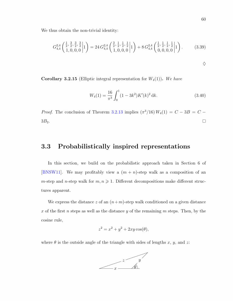
60
We thus obtain the non-trivial identity:
G2,44,4
(12, 3
2, 3
2, 3
2
1, 0, 0, 0
∣∣∣∣1) = 24G2,44,4
(32, 1
2, 1
2, 1
2
1, 0, 0, 0
∣∣∣∣1)+ 8G2,44,4
(12, 1
2, 1
2, 1
2
0, 0, 0, 0
∣∣∣∣1) . (3.39)
♦
Corollary 3.2.15 (Elliptic integral representation for W4(1)). We have
W4(1) =16
π3
∫ 1
0
(1− 3k2)K ′(k)2 dk. (3.40)
Proof. The conclusion of Theorem 3.2.13 implies (π3/16)W4(1) = C − 3B = C −
3B2.
3.3 Probabilistically inspired representations
In this section, we build on the probabilistic approach taken in Section 6 of
[BNSW11]. We may profitably view a (m + n)-step walk as a composition of an
m-step and n-step walk for m,n > 1. Different decompositions make different struc-
tures apparent.
We express the distance z of an (n+m)-step walk conditioned on a given distance
x of the first n steps as well as the distance y of the remaining m steps. Then, by the
cosine rule,
z2 = x2 + y2 + 2xy cos(θ),
where θ is the outside angle of the triangle with sides of lengths x, y, and z:
\θx
zjjjjjjjjjjjjj
jjjjjjjjjjjjj y�����
�����

61
It follows that for s > 0, the s-th moment of an (n+m)-step walk conditioned on the
distance x of the first n steps and the distance y of the remaining m steps is
gs(x, y) :=1
π
∫ π
0
zs dθ = |x− y|s 2F1
(12,− s
2
1
∣∣∣∣− 4xy
(x− y)2
). (3.41)
Here we appealed to symmetry to restrict the angle to θ ∈ [0, π). We then evaluated
the integral in hypergeometric form which, for instance, can be done with the help of
Mathematica or Maple.
Remark 3.3.1 (Alternate forms for gs). Using Kummer’s quadratic transformation
[AAR99], we obtain
gs(x, y) = Re ys 2F1
(− s2,− s
2
1
∣∣∣∣x2
y2
)(3.42)
for general positive x, y. This provides an analytic continuation of s 7→ gs(x, y). In
particular, we have
g−1(x, y) =2
πRe
1
yK
(x
y
)(3.43)
and, with E the complete elliptic integral of the second kind, we have
g1(x, y) =2
πRe y
{2E
(x
y
)−(
1− x2
y2
)K
(x
y
)}. (3.44)
This later form has various re-expressions. ♦
Denote by pn(x) the density of the distance x for an n-step walk. Since Wn+m(s)
is the s-th moment of the distance of an (n+m)-step walk, we obtain
Wn+m(s) =
∫ n
0
∫ m
0
gs(x, y) pn(x)pm(y) dy dx, (3.45)
for s > 0. Since for the 1-step walk we have p1(x) = δ1(x), this generalizes the
corresponding formula given for Wn+1(s) in [BNSW11].
62
In (3.45), if n = 0, then we may take p0(x) = δ0(x), and regard the limits of
integration as from −ε and +ε, ε→ 0. Then gs = ys as the hypergeometric collapses
to 1, and we recover the basic form
Wm(s) =
∫ m
0
yspm(y) dy. (3.46)
It is also easily shown that the probability density for a 2-step walk is given by
p2(x) =2
π√
4− x2
for 0 6 x 6 2 and 0 otherwise.
The density p3(x) for 0 6 x 6 3 can be expressed by
p3(x) = Re
(√x
π2K
(√(x+ 1)3(3− x)
16x
)), (3.47)
see, e.g., [Pea06]. To make (3.47) more accessible we need the following cubic identity.
Proposition 3.3.2. For all 0 6 x 6 1 we have
K
(√16x3
(3− x)3(1 + x)
)=
3− x3 + 3x
K
(√16x
(3− x)(1 + x)3
).
Proof. Both sides satisfy the differential equation
4x2(x+3)2f(x)+(x−3)(x+1)2((x3−9x2−9x+9)f ′(x)+x(x3−x2−9x+9)f ′′(x)) = 0,
and both of their function values and derivative values agree at the origin.
Applying Jacobi’s imaginary transform [BB98, p. 73], Re K(x) = 1xK(
1x
), for

63
x > 1 to express p3(x) as a real function over [0, 1] and [1, 3], leads to
W3(−1) =
∫ 3
0
p3(x)
xdx =
4
π2
∫ 1
0
K(√
16x(3−x)(1+x)3
)√
(3− x)(1 + x)3dx+
1
π2
∫ 3
1
K
(√(3−x)(1+x)3
16x
)√x
dx.
The change of variables x→ 3−t1+t
in the last integral transforms it into the second
last integral. Therefore,
W3(−1) = 2
∫ 1
0
p3(x)
xdx. (3.48)
To make sense of this more abstractly, let
σ(x) =3− x1 + x
, λ(x) =(1 + x)3(3− x)
16x.
Then for 0 < x < 3 we have σ2(x) = x and λ(x)λ(σ(x)) = 1. In consequence σ is an
involution that sends [0, 1] to [1, 3] and
p3(x) =4x
(3− x)(x+ 1)p3(σ(x)). (3.49)
Example 3.3.3 (Series for p3 and W3(−1)). We know that
W3(2k) =k∑j=0
(k
j
)2(2j
j
)
is the sum of squares of trinomials (see (3.8) and [BNSW11]). Using Proposition
3.3.2, we may now apply equation (184) in [BBBG08, Section 5.10] to obtain
p3(x) =2x
π√
3
∞∑k=0
W3(2k)(x
3
)2k
, (3.50)
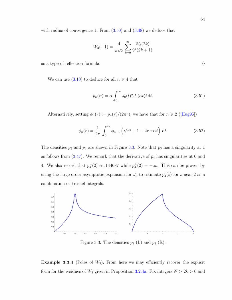
64
with radius of convergence 1. From (3.50) and (3.48) we deduce that
W3(−1) =4
π√
3
∞∑k=0
W3(2k)
9k(2k + 1)
as a type of reflection formula. ♦
We can use (3.10) to deduce for all n > 4 that
pn(α) = α
∫ ∞0
J0(t)nJ0(αt)t dt. (3.51)
Alternatively, setting φn(r) := pn(r)/(2πr), we have that for n > 2 ([Hug95])
φn(r) =1
2π
∫ 2π
0
φn−1
(√r2 + 1− 2r cos t
)dt. (3.52)
The densities p3 and p4 are shown in Figure 3.3. Note that p3 has a singularity at 1
as follows from (3.47). We remark that the derivative of p4 has singularities at 0 and
4. We also record that p−4 (2) ≈ .144687 while p+4 (2) = −∞. This can be proven by
using the large-order asymptotic expansion for Jν to estimate p′4(s) for s near 2 as a
combination of Fresnel integrals.
0.5 1.0 1.5 2.0 2.5 3.0
0.1
0.2
0.3
0.4
0.5
0.6
0.7
1 2 3 4
0.1
0.2
0.3
0.4
0.5
Figure 3.3: The densities p3 (L) and p4 (R).
Example 3.3.4 (Poles of W3). From here we may efficiently recover the explicit
form for the residues of W3 given in Proposition 3.2.4a. Fix integers N > 2k > 0 and
65
0 < α < 1. Use the series p3(x) =∑
j>0 ajx2j+1 in (3.50) to write
W3(s)−∫ 3
α
p3(x)xs dx−∫ α
0
∞∑j=N
ajx2j+1+s dx =
∫ α
0
N−1∑j=0
ajx2j+1+s dx
=N∑j=1
aj−1α2j+s
2j + s, (3.53)
and observe that both sides are holomorphic and so (3.53) holds in a neighborhood
of s = −2k. Since only the first term on the left has a pole at −2k we may deduce
that Res(−2k)(W3) = ak−1. Equivalently,
Res(−2k−2)(W3) =2
π√
3
W3(2k)
32k,
which exposes an elegant reflection property. ♦
Remark 3.3.5 (W5). Using (3.45) we may express W5(s) and W6(s) as double inte-
grals, for example,
W5(−1) =4
π4
∫ 3
0
∫ 2
0
√x
y√
4− y2Re
(K
(x
y
))Re
(K
(√(x+ 1)3(3− x)
16x
))dy dx.
We also have an expression based on taking two 2-step walks and a 1-step walk:
W5(−1) =8
π4
∫ 2
0
∫ 2
0
∫ π
0
Re K(√x2 + y2 + 2xy cos z)√
(4− x2)(4− y2)dz dx dy
=8
π4
∫ π2
0
∫ π2
0
∫ π
0
Re K(
2√
sin2 a+ sin2 b+ 2 sin a sin b cos c)
dc da db,
but we have been unable to make further progress with these forms. ♦

66
3.3.1 Elliptic integral representations
From (3.45), we derive
W4(s) =2s+2
π2
∫ 1
0
∫ 1
0
gs(x, y)√(1− x2)(1− y2)
dx dy
=2s+2
π2
∫ π/2
0
∫ π/2
0
gs(sinu, sin v) du dv.
where s > −2. In particular, for s = −1, again using Jacobi’s imaginary transforma-
tion, we have:
W4(−1) =4
π3Re
∫ 1
0
∫ 1
0
K(x/y)
y√
(1− x2)(1− y2)dx dy (3.54)
=8
π3
∫ 1
0
∫ 1
0
K(t)√(1− t2y2)(1− y2)
dy dt
=8
π3
∫ 1
0
K2(k) dk. (3.55)
The corresponding integral at s = 1 is
W4(1) =32
π3
∫ 1
0
(k + 1)(K(k)− E(k))
k2E
(2√k
k + 1
)dk.
Starting with Nesterenko’s theorem [Nes03] we have the following:
W4(−1) =1
2π3
∫[0,1]3
dxdydz√xyz(1− x)(1− y)(1− z)(1− x(1− yz))
. (3.56)
(Such integrals are related to Beukers’ integrals, which were used in the elementary
derivation of the irrationality of ζ(3).) Upon computing the dx integral, followed by

67
the change of variable k2 = yz, we have:
W4(−1) =1
π3
∫ 1
0
∫ 1
0
K(√
1− yz)√yz(1− y)(1− z)
dy dz (3.57)
=2
π3
∫ 1
0
∫ 1
k2
K(√
1− k2)√y(1− y)(y − k2)
dy dk
=4
π3
∫ 1
0
K ′(k)2 dk. (3.58)
Compare this with the corresponding (3.54). In particular, appealing to Theorem
3.2.11 we derive the closed forms:
2
∫ 1
0
K(k)2 dk =
∫ 1
0
K ′(k)2 dk =(π
2
)4
7F6
( 54, 1
2, 1
2, 1
2, 1
2, 1
2, 1
214, 1, 1, 1, 1, 1
∣∣∣∣1) . (3.59)
Recalling Corollary 3.2.15 and equation (3.37) we also deduce that
W4(1) =96
π3
∫ 1
0
E ′(k)K ′(k) dk − 8W4(−1). (3.60)
If we make a trigonometric change of variables in (3.57), we obtain
W4(−1) =4
π3
∫ π/2
0
∫ π/2
0
K
(√1− sin2 x sin2 y
)dx dy. (3.61)
We may rewrite the integrand as a sum, and then interchange integration and sum-
mation to arrive at a slowly convergent representation of the same general form as in
Conjecture 3.1.1:
W4(−1) =1
2
∞∑n=0
(−1/2
n
)2
3F2
(12, 1
2,−n
1, 1
∣∣∣∣1) . (3.62)
Remark 3.3.6 (Relation to Watson integrals). From the evaluation (3.7) we note
that W3(−1) equals twice the second of three triple integrals considered by Watson

68
in [Wat38]:
W3(−1) =1
π3
∫ π
0
∫ π
0
∫ π
0
dudvdw
3− cos v cosw − cosw cosu− cosu cos v. (3.63)
This is derived in [BBG04] and various related extensions are to be found in [BBBG08].
It is not clear how to generalize this to W4(−1).
Watson’s second integral (3.63) also gives the alternative representation:
W3(−1) = π−5/2G3,23,3
(12, 1
2, 1
2
0, 0, 0
∣∣∣∣4) . (3.64)
The equivalence of this and the Meijer G representation coming from Theorem 3.2.7
can be established similarly to the proof of Theorem 3.2.11 upon using the Meijer G
transformation
Gm,np,q
(a
b
∣∣∣∣x) = Gn,mq,p
(1− b
1− a
∣∣∣∣1x). (3.65)
♦
Remark 3.3.7 (Probability of return to the unit disk). By a simple geometric argu-
ment, there is a 13
chance of returning to the unit disk in a 2-step walk. Similarly, for
a 3-step walk, if the second step makes an angle θ with the first step, then the third
step can only vary over a range of θ to return to the unit disk (it can be parallel to
the first step, to the second step, or anywhere in between). Thus the probability of
returning to the unit disk in three steps is
1
4π2
∫ π
−π|θ| dθ =
1
4=
∫ 1
0
p3(x) dx.
Appealing to (3.50) we deduce that
∞∑k=0
W3(2k)
9k(k + 1)=
√3π
4.

69
In fact, as Kluyver showed [Klu06], the probability of an n-step walk ending in the
unit disk is 1/(n + 1). This is easily obtained by setting α = 1 in (3.10). See also
[Ber10] for a very short proof of this fact which is not based on a Bessel integral
representation. ♦
3.4 Partial resolution of Conjecture 3.1.1
We may now investigate Conjecture 3.1.1 which is restated below for convenience.
Conjecture. For positive integers n and complex s,
W2n(s)?[1]=∑j>0
(s/2
j
)2
W2n−1(s− 2j). (3.66)
We can resolve this conjecture modulo a conjectured technical estimate given in
Conjecture 3.4.2. The proof outline below certainly explains Conjecture 3.1.1 by
identifying the terms of the infinite sum as natural residues.
Proof. Using (3.17) we write W2n as a Bessel integral
W2n(−s) = 21−sΓ(1− s/2)
Γ(s/2)
∫ ∞0
xs−1J2n0 (x) dx.
Then we apply Theorem 3.2.6 to J2n0 = J2n−1
0 ·J0 for s in a vertical strip. Since, again
by (3.17), we have
∫ ∞0
xs−1J2n0 (x) dx = 2s−1 Γ(s/2)
Γ(1− s/2)Wn(−s)

70
we obtain
W2n(−s) = 21−sΓ(1− s/2)
Γ(s/2)
∫ ∞0
xs−1J2n−10 (x) · J0(x) dx (3.67)
=Γ(1− s/2)
Γ(s/2)
1
2πi
∫ δ+i∞
δ−i∞
1
2
Γ(z/2)Γ(s/2− z/2)
Γ(1− z/2)Γ(1− s/2 + z/2)W2n−1(−z) dz
where 0 < δ < 1.
Observe that the integrand has poles at z = s, s+2, s+4, . . . coming from Γ(s/2−
z/2) as well as (irrelevant for current purposes) poles at z = 0,−2,−4, . . . coming
from Γ(z/2). On the other hand, the term W2n−1(−z) has at most simple poles at
z = 2, 4, 6, . . . which are cancelled by the corresponding zeros of Γ(1 − z/2). This
asserted pole structure of W2n−1 was shown in Example 3.2.5 for n = 3 and may be
shown analogously for each n = 4, 5, . . . based on Proposition 3.2.4. That this works
generally is stated as Conjecture 3.4.1 below.
Next, we determine the residue of the integrand at z = s+ 2j. Since Γ(s/2− z/2)
has a residue of −2(−1)j/j! at z = s+ 2j, the residue of the integrand is
− (−1)jΓ(s/2 + j)
(j!)2Γ(1− s/2− j)W2n−1(−(2j + s)) = − Γ(s/2)
Γ(1− s/2)
(−s/2j
)2
W2n−1(−s− 2j).
Thus it follows that
W2n(−s) =∑j>0
(−s/2j
)2
W2n−1(−s− 2j), (3.68)
which is what we want to prove, provided that the contour of the integral after (3.67)
can be closed in the right half-plane. This is Conjecture 3.4.2 below.
This proof is thus rigorous provided that the next two conjectures hold. However,
note that Conjecture 3.4.1 is easily checked for individual n. In particular, it is true
for 2n− 1 6 45.

71
Conjecture 3.4.1 (Poles of W2n−1). For each n > 1 all poles of W2n−1 are simple.
Conjecture 3.4.2 (Growth of W2n−1). For given s,
lim infr→∞
∫γr
Γ(z/2)Γ(s/2− z/2)
Γ(1− z/2)Γ(1− s/2 + z/2)W2n−1(−z) dz = 0,
where γr is a right half-circle of radius r around δ ∈ (0, 1).
Remark 3.4.3 (Other approaches to Conjecture 3.1.1). We restrict ourself to the
core case with n = 2. One can prove that both sides of the needed identity satisfy the
recursion for W4. Hence, it suffices to show that the conjecture is correct for s = ±1.
Working entirely formally with (3.11) and ignoring the restriction on s we have:
∑j>0
(−1/2
j
)2
W3(−1− 2j) =∞∑j=0
(−1/2
j
)2
2−2jΓ(12− j)
Γ(12
+ j)
∫ ∞0
x2jJ30 (x) dx
=
∫ ∞0
J30 (x)
∞∑j=0
(−1/2
j
)2 Γ(12− j)
Γ(12
+ j)
(x2
)2j
dx
=
∫ ∞0
J40 (x) dx
= W4(−1),
on appealing to Example 3.2.1, since
∞∑j=0
(−1/2
j
)2 Γ(12− j)
Γ(12
+ j)x2j = J0(2x)
for x > 0. There is a corresponding manipulation for s = 1, but we cannot make
them rigorous. However, in [BSWZ11], we prove the conjecture for n = 2 and s an
integer. ♦

72
Conclusion
In addition to the two new conjectures made explicit above, it would be fascinating
to obtain closed forms for any of the residues in Proposition 3.2.4 with n > 5. It would
likewise be very informative to obtain a closed form for W5(±1).

73
Chapter 4
Densities of short uniform randomwalks
The contents of this chapter (apart from minor corrections or adaptions) have
been published as:
[BSWZ11] Densities of short uniform random walks(with Jonathan M. Borwein, James Wan, Wadim Zudilin (appendix by Don Zagier))
to appear in Canadian Journal of Mathematics
Abstract We study the densities of uniform random walks in the plane. A special
focus is on the case of short walks with three or four steps and less completely those
with five steps. As one of the main results, we obtain a hypergeometric representation
of the density for four steps, which complements the classical elliptic representation
in the case of three steps. It appears unrealistic to expect similar results for more
than five steps. New results are also presented concerning the moments of uniform
random walks and, in particular, their derivatives. Relations with Mahler measures
are discussed.
4.1 Introduction
An n-step uniform random walk is a walk in the plane that starts at the origin
and consists of n steps of length 1 each taken into a uniformly random direction.

74
The study of such walks largely originated with Pearson more than a century ago
[Pea05a, Pea05b, Pea06] who posed the problem of determining the distribution of
the distance from the origin after a certain number of steps. In this paper, we study
the (radial) densities pn of the distance travelled in n steps. This continues research
commenced in [BNSW11, BSW11] where the focus was on the moments of these
distributions:
Wn(s) :=
∫ n
0
pn(t)ts dt.
The densities for walks of up to 8 steps are depicted in Figure 4.1. As established
by Lord Rayleigh [Ray05], pn quickly approaches the probability density 2xne−x
2/n for
large n. This limiting density is superimposed in Figure 4.1 for n > 5.
0.5 1.0 1.5 2.0 2.5 3.0
0.1
0.2
0.3
0.4
0.5
0.6
0.7
(a) p3
1 2 3 4
0.1
0.2
0.3
0.4
0.5
(b) p4
1 2 3 4 5
0.05
0.10
0.15
0.20
0.25
0.30
0.35
(c) p5
1 2 3 4 5 6
0.05
0.10
0.15
0.20
0.25
0.30
0.35
(d) p6
1 2 3 4 5 6 7
0.05
0.10
0.15
0.20
0.25
0.30
(e) p7
2 4 6 8
0.05
0.10
0.15
0.20
0.25
0.30
(f) p8
Figure 4.1: Densities pn with the limiting behaviour superimposed for n > 5.
Closed forms were only known in the cases n = 2 and n = 3. The evaluation, for
0 6 x 6 2,
p2(x) =2
π√
4− x2(4.1)

75
is elementary. On the other hand, the density p3(x) for 0 6 x 6 3 can be expressed
in terms of elliptic integrals by
p3(x) = Re
(√x
π2K
(√(x+ 1)3(3− x)
16x
)), (4.2)
see, e.g., [Pea06]. One of the main results of this paper is a closed form evaluation of
p4 as a hypergeometric function given in Theorem 4.4.9. In (4.20) we also provide a
single hypergeometric closed form for p3 which, in contrast to (4.2), is real and valid
on all of [0, 3]. For convenience, we list these two closed forms here:
p3(x) =2√
3
π
x
(3 + x2)2F1
(13, 2
3
1
∣∣∣∣x2 (9− x2)2
(3 + x2)3
), (4.3)
p4(x) =2
π2
√16− x2
xRe 3F2
(12, 1
2, 1
256, 7
6
∣∣∣∣(16− x2)3
108x4
). (4.4)
We note that while Maple handled these well to high precision, Mathematica strug-
gled, especially with the analytic continuation of the 3F2 when the argument is greater
than 1.
A striking feature of the 3- and 4-step random walk densities is their modularity.
It is this circumstance which not only allows us to express them via hypergeometric
series, but also makes them a remarkable object of mathematical study.
This paper is structured as follows: In Section 4.2 we give general results for
the densities pn and prove for instance that they satisfy certain linear differential
equations. In Sections 4.3, 4.4, and 4.5 we provide special results for p3, p4, and p5
respectively. Particular interest is taken in the behaviour near the points where the
densities fail to be smooth. In Section 4.6 we study the derivatives of the moment
function and make a connection to multidimensional Mahler measures. Finally in
Section 4.7 we provide some related new evaluations of moments and so resolve a
central case of an earlier conjecture on convolutions of moments in [BSW11].

76
The amazing story of the appearance of Theorem 4.2.7 is worth mentioning here.
The theorem was a conjecture in an earlier version of this manuscript, and one of the
present authors communicated it to D. Zagier. That author was surprised to learn
that Zagier had already been asked for a proof of exactly the same identities a little
earlier, by P. Djakov and B. Mityagin.
Those authors had in fact proved the theorem already in 2004 (see [DM04, Theo-
rem 4.1] and [DM07, Theorem 8]) during their study of the asymptotics of the spectral
gaps of a Schrodinger operator with a two-term potential — their proof was indirect,
so that we should never have come across the identities without the accident of ask-
ing the same person the same question! Djakov and Mityagin asked Zagier about the
possibility of a direct proof of their identities (the subject of Theorem 4.2.7), and he
gave a very neat and purely combinatorial answer. It is this proof which is herein
presented in the Appendix.
We close this introduction with a historical remark illustrating the fascination
arising from these densities and their curious geometric features. H. Fettis devotes
the entire paper [Fet63] to proving that p5 is not linear on the initial interval [0, 1] as
ruminated upon by Pearson [Pea06]. This will be explained in Section 4.5.
4.2 The densities pn
It is a classical result of Kluyver [Klu06] that pn has the following Bessel integral
representation:
pn(x) =
∫ ∞0
xtJ0(xt)Jn0 (t) dt. (4.5)
Here Jν is the Bessel function of the first kind of order ν.
Remark 4.2.1. Equation (4.5) naturally generalizes to the case of nonuniform step
lengths. In particular, for n = 2 and step lengths a and b we record (see [Wat41,

77
p. 411] or [Hug95, 2.3.2]; the result is attributed to Sonine) that the corresponding
density is
p2(x; a, b) =
∫ ∞0
xtJ0(xt)J0(at)J0(bt) dt
=2x
π√
((a+ b)2 − x2)(x2 − (a− b)2)(4.6)
for |a− b| 6 x 6 a+ b and p2(x; a, b) = 0 otherwise. Observe how (4.6) specializes to
(4.1) in the case a = b = 1.
In the case n = 3 the density p3(x; a, b, c) has been evaluated by Nicholson [Wat41,
p. 414] in terms of elliptic integrals directly generalizing (4.2). The corresponding
extensions for four and more variables appear much less accessible. ♦
It is visually clear from the graphs in Figure 4.1 that pn is getting smoother for
increasing n. This can be made precise from (4.5) using the asymptotic formula for
J0 for large arguments and dominated convergence:
Theorem 4.2.2. For each integer n > 0, the density pn+4 is bn/2c times continuously
differentiable.
On the other hand, we note from Figure 4.1 that the only points preventing pn
from being smooth appear to be integers. This will be made precise in Theorem 4.2.4.
To this end, we recall a few things about the s-th moments Wn(s) of the density
pn which are given by
Wn(s) =
∫ ∞0
xspn(x) dx =
∫[0,1]n
∣∣∣∣∣n∑k=1
e2πxki
∣∣∣∣∣s
dx. (4.7)
Starting with the right-hand side, these moments had been investigated in [BNSW11,
BSW11]. There it was shown that Wn(s) admits an analytic continuation to all of

78
the complex plane with poles of at most order two at certain negative integers. In
particular, W3(s) has simple poles at s = −2,−4,−6, . . . and W4(s) has double poles
at these integers [BNSW11, Thm. 6, Ex. 2 & 3].
Moreover, from the combinatorial evaluation
Wn(2k) =∑
a1+···+an=k
(k
a1, . . . , an
)2
(4.8)
for integers k > 0 it followed that Wn(s) satisfies a functional equation, as in
[BNSW11, Ex. 1], coming from the inevitable recursion that exists for the right-
hand side of (4.8) . For instance,
(s+ 4)2W3(s+ 4)− 2(5s2 + 30s+ 46)W3(s+ 2) + 9(s+ 2)2W3(s) = 0,
and equation (4.9) below.
The first part of equation (4.7) can be rephrased as saying that Wn(s − 1) is
the Mellin transform of pn ([ML86]). We denote this by Wn(s − 1) = M [pn; s].
Conversely, the density pn is the inverse Mellin transform of Wn(s − 1). We intend
to exploit this relation as detailed for n = 4 in the following example.
Example 4.2.3 (Mellin transforms). For n = 4, the moments W4(s) satisfy the
functional equation
(s+ 4)3W4(s+ 4)− 4(s+ 3)(5s2 + 30s+ 48)W4(s+ 2) + 64(s+ 2)3W4(s) = 0. (4.9)
Recall the following rules for the Mellin transform: if F (s) = M [f ; s] then in the
appropriate strips of convergence
• M [xµf(x); s] = F (s+ µ),
• M [Dxf(x); s] = −(s− 1)F (s− 1).
79
Here, and below, Dx denotes differentiation with respect to x, and, for the second
rule to be true, we have to assume, for instance, that f is continuously differentiable.
Thus, purely formally, we can translate the functional equation (4.9) of W4 into
the differential equation A4 · p4(x) = 0 where A4 is the operator
A4 = x4(θ + 1)3 − 4x2θ(5θ2 + 3) + 64(θ − 1)3 (4.10)
= (x− 4)(x− 2)x3(x+ 2)(x+ 4)D3x + 6x4
(x2 − 10
)D2x (4.11)
+ x(7x4 − 32x2 + 64
)Dx +
(x2 − 8
) (x2 + 8
).
Here θ = xDx. However, it should be noted that p4 is not continuously differentiable.
Moreover, p4(x) is approximated by a constant multiple of√
4− x as x → 4− (see
Theorem 4.4.1) so that the second derivative of p4 is not even locally integrable. In
particular, it does not have a Mellin transform in the classical sense. ♦
Theorem 4.2.4. Let an integer n > 1 be given.
• The density pn satisfies a differential equation of order n− 1.
• If n is even (respectively odd) then pn is real analytic except at 0 and the even
(respectively odd) integers m ≤ n.
Proof. As illustrated for p4 in Example 4.2.3, we formally use the Mellin transform
method to translate the functional equation of Wn into a differential equation An ·
y(x) = 0. Since pn is locally integrable and compactly supported, it has a Mellin
transform in the distributional sense as detailed for instance in [ML86]. It follows
rigorously that pn solves An · y(x) = 0 in a distributional sense. In other words, pn
is a weak solution of this differential equation. The degree of this equation is n − 1
because the functional equation satisfied by Wn has coefficients of degree n − 1 as
shown in [BNSW11, Thm. 1].

80
The leading coefficient of the differential equation (in terms of Dx as in (4.11))
turns out to be
xn−1∏
2|(m−n)
(x2 −m2) (4.12)
where the product is over the even or odd integers 1 ≤ m ≤ n depending on whether
n is even or odd. This is discussed below in Section 4.2.1.
Thus the leading coefficient of the differential equation is nonzero on [0, n] except
for 0 and the even or odd integers already mentioned. On each interval not containing
these points it follows, as described for instance in [Hor89, Cor. 3.1.6], that pn is
in fact a classical solution of the differential equation. Moreover the analyticity of
the coefficients, which are polynomials in our case, implies that pn is piecewise real
analytic as claimed.
Remark 4.2.5. It is one of the basic properties of the Mellin transform, see for
instance [FS09, Appendix B.7], that the asymptotic behaviour of a function at zero is
determined by the poles of its Mellin transform which lie to the left of the fundamental
strip. It is shown in [BNSW11] that the poles of Wn(s) occur at specific negative
integers and are at most of second order. This translates into the fact that pn has an
expansion at 0 as a power series with additional logarithmic terms in the presence of
double poles. This is made explicit in the case of p4 in Example 4.4.3.
4.2.1 An explicit recursion
We close this section by providing details for the claim made in (4.12). Recall
that the even moments fn(k) := Wn(2k) satisfy a recurrence of order λ := dn/2e with
polynomial coefficients of degree n− 1 (see [BNSW11]). An entirely explicit formula
for this recurrence is given in [Ver04]:

81
Theorem 4.2.6.
∑j>0
kn+1∑
α1,...,αj
j∏i=1
(−αi)(n+ 1− αi)(
k − ik − i+ 1
)αi−1 fn(k − j) = 0 (4.13)
where the sum is over all sequences α1, . . . , αj such that 0 6 αi 6 n and αi+1 6 αi−2.
Observe that (4.12) is easily checked for each fixed n by applying Theorem 4.2.6.
We explicitly checked the cases n 6 1000 (using a recursive formulation of Theorem
4.2.6 from [Ver04]) while only using this statement for n 6 5 in this paper. The fact
that (4.12) is true in general is recorded and made more explicit in Theorem 4.2.7
below.
For fixed n, write the recurrence for fn(k) in the form∑n−1
j=0 kjqj(K) where qj
are polynomials and K is the shift k → k + 1. Then qn−1 is the characteristic
polynomial of this recurrence, and, by the rules outlined in Example 4.2.3, we find
that the differential equation satisfied by pn(x) is of the form qn−1(x2)θn−1 + · · · ,
where θ = xDx and the dots indicate terms of lower order in θ.
We claim that the characteristic polynomial of the recurrence (4.13) satisfied by
fn(k) is∏
2|(m−n)(x − m2) where the product is over the integers 1 ≤ m ≤ n such
that m ≡ n modulo 2. This implies (4.12). By Theorem 4.2.6 the characteristic
polynomial isλ∑j=0
∑α1,...,αj
j∏i=1
(−αi)(n+ 1− αi)
xλ−j (4.14)
where λ = dn/2e and the sum is again over all sequences α1, . . . , αj such that 0 6
αi 6 n and αi+1 6 αi − 2. The claimed evaluation is thus equivalent to the following
identity, first proven by P. Djakov and B. Mityagin [DM04, DM07]. Zagier’s more
direct and purely combinatorial proof is given in the Appendix.

82
Theorem 4.2.7. For all integers n, j > 1,
∑06m1,...,mj<n/2
mi<mi+1
j∏i=1
(n− 2mi)2 =
∑16α1,...,αj6nαi6αi+1−2
j∏i=1
αi(n+ 1− αi). (4.15)
4.3 The density p3
The elliptic integral evaluation (4.2) of p3 is very suitable to extract information
about the features of p3 exposed in Figure 4.1(a). It follows, for instance, that p3 has
a singularity at 1. Moreover, using the known asymptotics for K(x), we may deduce
that the singularity is of the form
p3(x) =3
2π2log
(4
|x− 1|
)+O(1) (4.16)
as x→ 1.
We also recall from [BSW11, Ex. 5] that p3 has the expansion, valid for 0 6 x 6 1,
p3(x) =2x
π√
3
∞∑k=0
W3(2k)(x
3
)2k
(4.17)
where
W3(2k) =k∑j=0
(k
j
)2(2j
j
)(4.18)
is the sum of squares of trinomials. Moreover, we have from [BSW11, Eqn. 29] the
functional relation
p3(x) =4x
(3− x)(x+ 1)p3
(3− x1 + x
)(4.19)
so that (4.17) determines p3 completely and also makes apparent the behaviour at 3.
We close this section with two more alternative expressions for p3.
83
Example 4.3.1 (Hypergeometric form for p3). Using the techniques in [CZ10] we
can deduce from (4.17) that
p3(x) =2√
3x
π (3 + x2)2F1
(1
3,2
3; 1;
x2 (9− x2)2
(3 + x2)3
)(4.20)
which is found in a similar but simpler way than the hypergeometric form of p4 given
in Theorem 4.4.9. Once obtained, this identity is easily proven using the differential
equation from Theorem 4.2.4 satisfied by p3. From (4.20) we see, for example, that
p3(√
3)2 = 32π2W3(−1). ♦
Example 4.3.2 (Iterative form for p3). The expression (4.20) can be interpreted in
terms of the cubic AGM, AG3, see [BB91], as follows. Recall that AG3(a, b) is the
limit of iterating
an+1 =an + 2bn
3, bn+1 = 3
√bn
(a2n + anbn + b2
n
3
),
beginning with a0 = a and b0 = b. The iterations converge cubically, thus allowing
for very efficient high-precision evaluation. On the other hand,
1
AG3(1, s)= 2F1
(1
3,2
3; 1; 1− s3
)
so that in consequence of (4.20), for 0 6 x 6 3,
p3(x) =2√
3
π
x
AG3(3 + x2, 3 |1− x2|2/3). (4.21)
Note that p3(3) =√
32π
is a direct consequence of the final formula.
Finally we remark that the cubic AGM also makes an appearance in the case
n = 4. We just mention that the modular properties of p4 recorded in Remark 4.4.11

84
can be stated in terms of the theta functions
b(τ) =η(τ)3
η(3τ), c(τ) = 3
η(3τ)3
η(τ)(4.22)
where η is the Dedekind eta function defined in (4.42). For more information and
proper definitions of the functions b, c as well as a, which is related by a3 = b3 +c3, we
refer to [BBG94]. Ultimately we are hopeful that, in search for an analogue of (4.19)
for p4, this may lead to an algebraic relation between algebraically related arguments
of p4. ♦
4.4 The density p4
The densities pn are recursively related. As in [Hug95], setting φn(x) = pn(x)/(2πx),
we have that for integers n > 2
φn(x) =1
2π
∫ 2π
0
φn−1
(√x2 − 2x cosα + 1
)dα. (4.23)
We use this recursive relation to get some quantitative information about the
behaviour of p4 at x = 4.
Theorem 4.4.1. As x→ 4−,
p4(x) =
√2
π2
√4− x− 3
√2
16π2(4− x)3/2 +
23√
2
512π2(4− x)5/2 +O
((4− x)7/2
).
Proof. Set y =√x2 − 2x cosα + 1. For 2 < x < 4,
φ4(x) =1
π
∫ π
0
φ3(y) dα =1
π
∫ arccos(x2−82x
)
0
φ3(y) dα

85
since φ3 is only supported on [0, 3]. Note that φ3(y) is continuous and bounded in the
domain of integration. By the Leibniz integral rule, we can thus differentiate under
the integral sign to obtain
φ′4(x) = − 1
π
(x2 + 8)φ3(3)
x√
(16− x2)(x2 − 4)+
1
π
∫ arccos(x2−82x
)
0
(x− cos(α))φ′3(y)
ydα. (4.24)
This shows that φ′4, and hence p′4, have a singularity at x = 4. More specifically,
φ′4(x) = − 1
8√
2π3√
4− x+O(1) as x→ 4−.
Here, we used that φ3(3) =√
312π2 . It follows that
p′4(x) = − 1√2π2√
4− x+O(1)
which, upon integration, is the claim to first order. Differentiating (4.24) twice more
proves the claim.
Remark 4.4.2. The situation for the singularity at x = 2+ is more complicated since
in (4.24) both the integral (via the logarithmic singularity of φ3 at 1, see (4.16)) and
the boundary term contribute. Numerically, we find, as x→ 2+,
p′4(x) = − 2
π2√x− 2
+O(1).
On the other hand, the derivative of p4 at 2 from the left is given by
p′4(2−) =
√3
π3F2
(−12, 1
3, 2
3
1, 1
∣∣∣∣1)− 2
3p4(2).
These observations can be proven in hindsight from Theorem 4.4.7. ♦
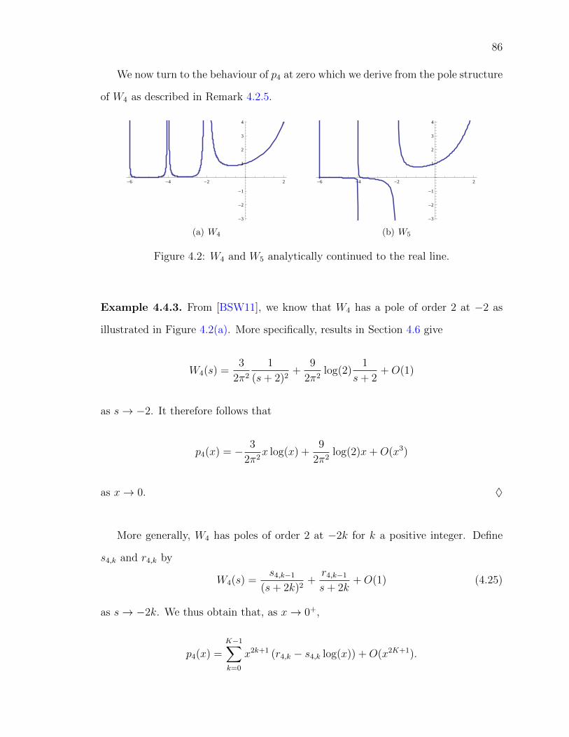
86
We now turn to the behaviour of p4 at zero which we derive from the pole structure
of W4 as described in Remark 4.2.5.
-6 -4 -2 2
-3
-2
-1
1
2
3
4
(a) W4
-6 -4 -2 2
-3
-2
-1
1
2
3
4
(b) W5
Figure 4.2: W4 and W5 analytically continued to the real line.
Example 4.4.3. From [BSW11], we know that W4 has a pole of order 2 at −2 as
illustrated in Figure 4.2(a). More specifically, results in Section 4.6 give
W4(s) =3
2π2
1
(s+ 2)2+
9
2π2log(2)
1
s+ 2+O(1)
as s→ −2. It therefore follows that
p4(x) = − 3
2π2x log(x) +
9
2π2log(2)x+O(x3)
as x→ 0. ♦
More generally, W4 has poles of order 2 at −2k for k a positive integer. Define
s4,k and r4,k by
W4(s) =s4,k−1
(s+ 2k)2+r4,k−1
s+ 2k+O(1) (4.25)
as s→ −2k. We thus obtain that, as x→ 0+,
p4(x) =K−1∑k=0
x2k+1 (r4,k − s4,k log(x)) +O(x2K+1).

87
In fact, knowing that p4 solves the linear Fuchsian differential equation (4.10) with a
regular singularity at 0 we may conclude:
Theorem 4.4.4. For small values x > 0,
p4(x) =∞∑k=0
(r4,k − s4,k log(x)) x2k+1. (4.26)
Note that
s4,k =3
2π2
W4(2k)
82k
as the two sequences satisfy the same recurrence and initial conditions. The numbers
W4(2k) are also known as the Domb numbers ([BBBG08]), and their generating
function in hypergeometric form is given in [Rog09] and has been further studied in
[CZ10]. We thus have
∞∑k=0
s4,k x2k+1 =
6x
π2 (4− x2)3F2
(13, 1
2, 2
3
1, 1
∣∣∣∣ 108x2
(x2 − 4)3
)(4.27)
which is readily verified to be an analytic solution to the differential equation satisfied
by p4.
Remark 4.4.5. For future use, we note that (4.27) can also be written as
∞∑k=0
s4,k x2k+1 =
24x
π2 (16− x2)3F2
(13, 1
2, 2
3
1, 1
∣∣∣∣ 108x4
(16− x2)3
)(4.28)
which follows from the transformation
(1− 4x)3F2
(13, 1
2, 2
3
1, 1
∣∣∣∣− 108x
(1− 16x)3
)= (1− 16x)3F2
(13, 1
2, 2
3
1, 1
∣∣∣∣ 108x2
(1− 4x)3
)(4.29)
given in [CZ10, (3.1)]. ♦
88
On the other hand, as a consequence of (4.25) and the functional equation (4.9)
satisfied by W4, the residues r4,k can be obtained from the recurrence relation
128k3r4,k = 4(2k − 1)(5k2 − 5k + 2)r4,k−1 − 2(k − 1)3r4,k−2
+ 3(64k2s4,k − (20k2 − 20k + 6)s4,k−1 + (k − 1)2s4,k−2
)(4.30)
with r4,−1 = 0 and r4,0 = 92π2 log(2).
Remark 4.4.6. In fact, before realizing the connection between the Mellin transform
and the behaviour of p4 at 0, we empirically found that p4 on (0, 2) should be of the
form r(x) − s(x) log(x) where a and r are odd and analytic. We then numerically
determined the coefficients and observed the relation with the residues of W4 as given
in Theorem 4.4.4. ♦
The differential equation for p4 has a regular singularity at 0. A basis of solutions
at 0 can therefore be obtained via the Frobenius method, see for instance [Inc26].
Since the indicial equation has 1 as a triple root, the solution (4.27) is the unique
analytic solution at 0 while the other solutions have a logarithmic or double logarith-
mic singularity. The solution with a logarithmic singularity at 0 is explicitly given
in (4.34), and, from (4.26), it is clear that p4 on (0, 2) is a linear combination of the
analytic and the logarithmic solution.
Moreover, the differential equation for p4 is a symmetric square. In other words, it
can be reduced to a second order differential equation, which after a quadratic substi-
tution, has 4 regular singularities and is thus of Heun type. In fact, a hypergeometric
representation of p4 with rational argument is possible.
Theorem 4.4.7. For 2 < x < 4,
p4(x) =2
π2
√16− x2
x3F2
(12, 1
2, 1
256, 7
6
∣∣∣∣(16− x2)3
108x4
). (4.31)

89
Proof. Denote the right-hand side of (4.31) by q4(x) and observe that the hyperge-
ometric series converges for 2 < x < 4. It is routine to verify that q4 is a solution
of the differential equation A4 · y(x) = 0 given in (4.10) which is also satisfied by
p4 as proven in Theorem 4.2.4. Together with the boundary conditions supplied by
Theorem 4.4.1 it follows that p4 = q4.
We note that Theorem 4.4.7 gives 2√
16− x2/(π2x) as an approximation to p4(x)
near x = 4, which is much more accurate than the elementary estimates established
in Theorem 4.4.1.
Corollary 4.4.8. In particular,
p4(2) =27/3π
3√
3Γ
(2
3
)−6
=
√3
πW3(−1). (4.32)
Quite marvelously, as first discovered numerically:
Theorem 4.4.9. For 0 < x < 4,
p4(x) =2
π2
√16− x2
xRe 3F2
(12, 1
2, 1
256, 7
6
∣∣∣∣(16− x2)3
108x4
). (4.33)
Proof. To obtain the analytic continuation of the 3F2 for 0 < x < 2 we employ the
formula [Luk69, 5.3], valid for all z,
q+1Fq
(a1, . . . , aq+1
b1, . . . , bq
∣∣∣∣z) =
∏j Γ(bj)∏j Γ(aj)
q+1∑k=1
Γ(ak)∏
j 6=k Γ(aj − ak)∏j Γ(bj − ak)
(−z)−ak
× q+1Fq
(ak, {ak − bj + 1}j{ak − aj + 1}j 6=k
∣∣∣∣1z),
which requires the aj to not differ by integers. Therefore we apply it to
3F2
( 12
+ ε, 12, 1
2− ε
56, 7
6
∣∣∣∣z) .

90
and take the limit as ε→ 0. This ultimately produces, for z > 1,
Re 3F2
( 12, 1
2, 1
256, 7
6
∣∣∣∣z) =log(108z)
2√
3z3F2
(13, 1
2, 2
3
1, 1
∣∣∣∣1z)
(4.34)
+1
2√
3z
∞∑n=0
(13)n(1
2)n(2
3)n
n!3
(1
z
)n(5Hn − 2H2n − 3H3n).
Here Hn =∑n
k=1 1/k is the n-th harmonic number. Now, insert the appropriate
argument for z and the factors so the left-hand side corresponds to the claimed closed
form. Observing that (13
)n
(12
)n
(23
)n
=(2n)!(3n)!
108n(n!)2,
we thus find that the right-hand side of (4.33) is given by − log(x)S4(x) plus
6
π2
∞∑n=0
(2n)!(3n)!
(n!)5
x4n+1
(16− x2)3n
(5Hn − 2H2n − 3H3n + 3 log(16− x2)
)where S4 is the solution (analytic at 0) to the differential equation for p4 given in
(4.28). This combination can now be verified to be a formal and hence actual solution
of the differential equation for p4. Together with the boundary conditions supplied
by Theorem 4.4.4 this proves the claim.
Remark 4.4.10. Let us indicate how the hypergeometric expression for p4 given in
Theorem 4.4.7 was discovered. Consider the generating series
y0(z) =∞∑k=0
W4(2k)zk (4.35)
of the Domb numbers which is just a rescaled version of (4.27). Corresponding to
(4.28), the hypergeometric form for this series given in [Rog09] is
y0(z) =1
1− 4z3F2
(13, 1
2, 2
3
1, 1
∣∣∣∣ 108z2
(1− 4z)3
)(4.36)

91
which converges for |z| < 1/16. y0 satisfies the differential equation B4 · y0(z) = 0
where
B4 = 64z2(θ + 1)3 − 2z(2θ + 1)(5θ2 + 5θ + 2) + θ3 (4.37)
and θ = z ddz
. Up to a change of variables this is (4.10); y0 is the unique solution
which is analytic at zero and takes the value 1 at zero; the other solutions which are
not a multiple of y0 have a single or double logarithmic singularity. Let y1 be the
solution characterized by
y1(z)− y0(z) log(z) ∈ zQ[[z]]. (4.38)
Note that it follows from (4.38) as well as Theorem 4.4.4 together with the initial
values s4,0 = 32π2 and r4,0 = s4,0 log(8) that p4, for small positive argument, is given
by
p4(x) = − 3x
4π2y1
(x2
64
). (4.39)
If x ∈ (2, 4) and z = x2/64 then the argument t = 108z2
(1−4z)3of the hypergeometric
function in (4.36) takes the values (1,∞). We therefore consider the solutions of the
corresponding hypergeometric equation at infinity. A standard basis for these is
t−1/33F2
( 13, 1
3, 1
323, 5
6
∣∣∣∣1t), t−1/2
3F2
( 12, 1
2, 1
256, 7
6
∣∣∣∣1t), t−2/3
3F2
( 23, 2
3, 2
343, 7
6
∣∣∣∣1t). (4.40)
In fact, the second element suffices to express p4 on the interval (2, 4) as shown in
Theorem 4.4.7. ♦
We close this section by showing that, remarkably, p4 has modular structure.
Remark 4.4.11. As shown in [CZ10] the series y0 defined in (4.35) possesses the

92
modular parameterization
y0
(−η(2τ)6η(6τ)6
η(τ)6η(3τ)6
)=
η(τ)4η(3τ)4
η(2τ)2η(6τ)2. (4.41)
Here η is the Dedekind eta function defined as
η(τ) = q1/24
∞∏n=1
(1− qn) = q1/24
∞∑n=−∞
(−1)nqn(3n+1)/2, (4.42)
where q = e2πiτ . Moreover, the quotient of the logarithmic solution y1 defined in
(4.38) and y0 is related to the modular parameter τ used in (4.41) by
exp
(y1(z)
y0(z)
)= e(2τ+1)πi = −q. (4.43)
Combining (4.41), (4.43) and (4.39) one obtains the modular representation
p4
(8iη(2τ)3η(6τ)3
η(τ)3η(3τ)3
)=
6(2τ + 1)
πη(τ)η(2τ)η(3τ)η(6τ) (4.44)
valid when the argument of p4 is small and positive. This is the case for τ = −1/2 +
iy when y > 0. Remarkably, the argument attains the value 1 at the quadratic
irrationality τ = (√−5/3− 1)/2 (the 5/3rd singular value of the next section). As a
consequence, the value p4(1) has a nice evaluation which is given in Theorem 4.5.1.
♦
4.5 The density p5
As shown in [BSW11], W5(s) has simple poles at −2,−4, . . ., compare Figure
4.2(b). We write r5,k = Res−2k−2W5 for the residue of W5 at s = −2k − 2. A

93
surprising bonus is an evaluation of r5,0 = p4(1) ≈ 0.3299338011, the residue at
s = −2. This is because in general for n > 4, one has
Res−2Wn+1 = p′n+1(0) = pn(1),
as follows from [BSW11, Prop. 1(b)]; here p′n+1(0) denotes the derivative from the
right at zero.
Explicitly, using Theorem 4.4.9, we have,
r5,0 = p′5(0) =2√
15
π2Re 3F2
( 12, 1
2, 1
256, 7
6
∣∣∣∣125
4
). (4.45)
In fact, based on the modularity of p4 discussed in Remark 4.4.11 we find:
Theorem 4.5.1.
r5,0 =1
2π2
√Γ( 1
15)Γ( 2
15)Γ( 4
15)Γ( 8
15)
5Γ( 715
)Γ(1115
)Γ(1315
)Γ(1415
). (4.46)
Proof. The value τ = (√−5/3− 1)/2 in (4.44) gives the value p4(1) = r5,0. Applying
the Chowla–Selberg formula [SC67, BB98] to evaluate the eta functions yields the
claimed evaluation.
Using [BZ92, Table 4, (ii)], (4.46) may be simplified to
r5,0 =
√5
40
Γ( 115
)Γ( 215
)Γ( 415
)Γ( 815
)
π4(4.47)
=3√
5
π3
(√5− 1
)2
K215 =
√15
π3K5/3K15, (4.48)
where K15 and K5/3 are the complete elliptic integral at the 15th and 5/3rd singular
values [BB98].
Remarkably, these evaluations appear to extend to r5,1 ≈ 0.006616730259, the
residue at s = −4. Resemblance to the tiny nome of Bologna [BBBG08] led us to

94
discover — and then check to 400 places using (4.55) and (4.56) — that
r5,1?=
13
1800√
5
Γ( 115
)Γ( 215
)Γ( 415
)Γ( 815
)
π4− 1√
5
Γ( 715
)Γ(1115
)Γ(1315
)Γ(1415
)
π4. (4.49)
Using (4.47) this evaluation can be neatly restated as
r5,1?=
13
225r5,0 −
2
5π4
1
r5,0
. (4.50)
We summarize our knowledge as follows:
Theorem 4.5.2. The density p5 is real analytic on (0, 5) except at 1 and 3 and
satisfies the differential equation A5 · p5(x) = 0 where A5 is the operator
A5 = x6(θ + 1)4 − x4(35θ4 + 42θ2 + 3) (4.51)
+ x2(259(θ − 1)4 + 104(θ − 1)2)− (15(θ − 3)(θ − 1))2
and θ = xDx. Moreover, for small x > 0,
p5(x) =∞∑k=0
r5,k x2k+1 (4.52)
where
(15(2k + 2)(2k + 4))2 r5,k+2 =(259(2k + 2)4 + 104(2k + 2)2
)r5,k+1
−(35(2k + 1)4 + 42(2k + 1)2 + 3
)r5,k + (2k)4r5,k−1
(4.53)
with explicit initial values r5,−1 = 0 and r5,0, r5,1 given by (4.47) and (4.49) above.
Proof. First, the differential equation (4.51) is computed as was that for p4, see (4.10).
Next, as detailed in [BSW11, Ex. 3] the residues satisfy the recurrence relation (4.53)

95
with the given initial values. Finally, proceeding as for (4.26), we deduce that (4.52)
holds for small x > 0.
Numerically, the series (4.52) appears to converge for |x| < 3 which is in accor-
dance with 19
being a root of the characteristic polynomial of the recurrence (4.53);
see also (4.12). The series (4.52) is depicted in Figure 4.3.
0.5 1.0 1.5 2.0 2.5
0.2
0.4
0.6
0.8
Figure 4.3: The series (4.52) (dotted) and p5.
Since the poles of W5 are simple, no logarithmic terms are involved in (4.52) as
opposed to (4.26). In particular, by computing a few more residues from (4.53),
p5(x) = 0.329934x+ 0.00661673x3 + 0.000262333x5 + 0.0000141185x7 +O(x9)
near 0 (with each coefficient given to six digits of precision only), explaining the
strikingly straight shape of p5(x) on [0, 1]. This phenomenon was observed by Pearson
[Pea06] who stated that for p5(x)/x between x = 0 and x = 1,
“the graphical construction, however carefully reinvestigated, did not per-
mit of our considering the curve to be anything but a straight line. . . Even
if it is not absolutely true, it exemplifies the extraordinary power of such
integrals of J products [that is, (4.5)] to give extremely close approxima-
tions to such simple forms as horizontal lines.”

96
This conjecture was investigated in detail in [Fet63] wherein the nonlinearity was
first rigorously established. This work and various more recent papers highlight the
difficulty of computing the underlying Bessel integrals.
Remark 4.5.3. Recall from Example 4.4.3 that the asymptotic behaviour of pn at
zero is determined by the poles of the moments Wn(s). To obtain information about
the behaviour of pn(x) as x → n−, we consider the “reversed” densities pn(x) =
pn(n− x) and their moments Wn(s). For non-negative integers k,
Wn(k) =
∫ n
0
xkpn(x) dx =
∫ n
0
(n− x)kpn(x) dx =k∑j=0
(k
j
)(−1)jnk−jWn(j)
On the other hand, we can find a recurrence satisfied by the Wn(s) as follows: a
differential equation for the densities pn(x) is obtained from Theorem 4.2.4 by a
change of variables. The Mellin transform method as described in Example 4.2.3 then
provides a recurrence for the moments Wn(s). We next apply the same reasoning as
in [BSW11] to obtain information about the pole structure of Wn(s). It should be
emphasized that this involves knowledge about initial conditions in term of explicit
values of initial moments Wn(2k).
For instance, in the case n = 4, we find that the moments W4(s) have simple poles
at −32,−5
2,−7
2, . . . which predicts an expansion of p4(x) as given in Theorem 4.4.1.
For n = 5, we learn that W5(s) has simple poles at s = −2,−3,−4, . . .. It then
follows, as for (4.52), that p5(x) =∑∞
k=0 r5,k (x− 5)k+1 for x 6 5 and close to 5. The
r5,k are the residues of W5(s) at s = −k − 2. ♦
97
4.6 Derivative evaluations of Wn
As illustrated by Theorem 4.4.4, the residues of Wn(s) are very important for
studying the densities pn as they directly translate into behaviour of pn at 0. The
residues may be obtained as a linear combination of the values of Wn(s) and W ′n(s).
Example 4.6.1 (Residues of Wn). Using the functional equation for W3(s) and
L’Hopital’s rule we find that the residue at s = −2 can be expressed as
Res−2(W3) =8 + 12W ′
3(0)− 4W ′3(2)
9. (4.54)
This is a general principle and we likewise obtain for instance:
Res−2(W5) =16 + 1140W ′
5(0)− 804W ′5(2) + 64W ′
5(4)
225, (4.55)
Res−4(W5) =26 Res−2(W5)− 16− 20W ′
5(0) + 4W ′5(2)
225. (4.56)
In the presence of double poles, as for W4,
lims→−2
(s+ 2)2W4(s) =3 + 4W ′
4(0)−W ′4(2)
8(4.57)
and for the residue:
Res−2(W4) =9 + 18W ′
4(0)− 3W ′4(2) + 4W ′′
4 (0)−W ′′4 (2)
16. (4.58)
Equations (4.57, 4.58) are used in Example 4.4.3 and each unknown is evaluated
below. ♦
We are therefore interested in evaluations of the derivatives of Wn for even argu-
ments.

98
Example 4.6.2 (Derivatives of W3 and W4). Differentiating the double integral for
W3(s) (4.7) under the integral sign, we have
W ′3(0) =
1
2
∫ 1
0
∫ 1
0
log(4 sin(πy) cos(2πx) + 3− 2 cos(2πy)) dx dy.
Then, using
∫ 1
0
log(a+ b cos(2πx)) dx = log
(1
2
(a+√a2 − b2
))for a > b > 0,
we deduce
W ′3(0) =
∫ 5/6
1/6
log(2 sin(πy)) dy =1
πCl(π
3
), (4.59)
where Cl denotes the Clausen function. Knowing as we do that the residue at s = −2
is 2/(√
3π), we can thus also obtain from (4.54) that
W ′3(2) = 2 +
3
πCl(π
3
)− 3√
3
2π.
In like fashion,
W ′4(0) =
3
8π2
∫ π
0
∫ π
0
log (3 + 2 cosx+ 2 cos y + 2 cos(x− y)) dx dy
=7
2
ζ(3)
π2. (4.60)
The final equality will be shown in Example 4.6.6. Note that we may also write
W ′3(0) =
1
8π2
∫ 2π
0
∫ 2π
0
log(3 + 2 cos x+ 2 cos y + 2 cos(x− y)) dx dy.
99
The similarity between W ′3(0) and W ′
4(0) is not coincidental, but comes from applying
∫ 1
0
log((a+ cos 2πx)2 + (b+ sin 2πx)2
)dx =
log(a2 + b2) if a2 + b2 > 1,
0 otherwise
to the triple integral of W ′4(0). As this reduction breaks the symmetry, we cannot
apply it to W ′5(0) to get a similar integral. ♦
In general, differentiating the Bessel integral expression
Wn(s) = 2s+1−k Γ(1 + s2)
Γ(k − s2)
∫ ∞0
x2k−s−1
(−1
x
d
dx
)kJn0 (x) dx, (4.61)
obtained by David Broadhurst [Bro09] and discussed in [BSW11], under the integral
sign gives
W ′n(0) = n
∫ ∞0
(log
(2
x
)− γ)Jn−1
0 (x)J1(x) dx
= log(2)− γ − n∫ ∞
0
log(x)Jn−10 (x)J1(x) dx, (4.62)
where γ is the Euler-Mascheroni constant, and
W ′′n (0) = n
∫ ∞0
(log
(2
x
)− γ)2
Jn−10 (x)J1(x) dx.
Likewise
W ′n(−1) = (log(2)− γ)Wn(−1)−
∫ ∞0
log(x)Jn0 (x) dx,
and
W ′n(1) =
∫ ∞0
n
xJn−1
0 (x)J1(x) (1− γ − log(2x)) dx.
Remark 4.6.3. We may therefore obtain many identities by comparing the above

100
equations to known values. For instance,
3
∫ ∞0
log(x)J20 (x)J1(x) dx = log(2)− γ − 1
πCl(π
3
).
♦
Example 4.6.4 (Derivatives of W5). In the case n = 5,
W ′5(0) = 5
∫ ∞0
(log
(2
t
)− γ)J4
0 (t)J1(t) dt ≈ 0.54441256
with similar but more elaborate formulae for W ′5(2) and W ′
5(4). Observe that in
general we also have
W ′n(0) = log(2)− γ −
∫ 1
0
(Jn0 (x)− 1)dx
x−∫ ∞
1
Jn0 (x)dx
x, (4.63)
which is useful numerically. ♦
In fact, the hypergeometric representation of W3 and W4 first obtained in [Cra09]
and recalled below also makes derivation of the derivatives of W3 and W4 possible.
Corollary 4.6.5 (Hypergeometric forms). For s not an odd integer, we have
W3(s) =1
22s+1tan(πs
2
)( ss−1
2
)2
3F2
( 12, 1
2, 1
2s+3
2, s+3
2
∣∣∣∣14)
+
(ss2
)3F2
(− s2,− s
2,− s
2
1,− s−12
∣∣∣∣14),
(4.64)
and, if also Re s > −2, we have
W4(s) =1
22stan(πs
2
)( ss−1
2
)3
4F3
( 12, 1
2, 1
2, s
2+ 1
s+32, s+3
2, s+3
2
∣∣∣∣1)+
(ss2
)4F3
( 12,− s
2,− s
2,− s
2
1, 1,− s−12
∣∣∣∣1) .(4.65)
Example 4.6.6 (Evaluation of W ′3(0) and W ′
4(0)). If we write (4.64) or (4.65) as
Wn(s) = f1(s)F1(s) + f2(s)F2(s), where F1, F2 are the corresponding hypergeometric
101
functions, then it can be readily verified that f1(0) = f ′2(0) = F ′2(0) = 0. Thus,
differentiating (4.64) by appealing to the product rule we get:
W ′3(0) =
1
π3F2
( 12, 1
2, 1
232, 3
2
∣∣∣∣14)
=1
πCl(π
3
).
The last equality follows from setting θ = π/6 in the identity
2 sin(θ)3F2
( 12, 1
2, 1
232, 3
2
∣∣∣∣sin2 θ
)= Cl (2 θ) + 2 θ log (2 sin θ) .
Likewise, differentiating (4.65) gives
W ′4(0) =
4
π2 4F3
( 12, 1
2, 1
2, 1
32, 3
2, 3
2
∣∣∣∣1) =7ζ(3)
2π2, (4.66)
thus verifying (4.60). In this case the hypergeometric evaluation
4F3
( 12, 1
2, 1
2, 1
32, 3
2, 3
2
∣∣∣∣1) =∞∑n=0
1
(2n+ 1)3=
7
8ζ(3),
is elementary. ♦
Differentiating (4.64) at s = 2 leads to the evaluation
3F2
( 12, 1
2, 1
252, 5
2
∣∣∣∣14)
=27
4
(Cl(π
3
)−√
3
2
),
while from (4.65) at s = 2 we obtain
W ′4(2) = 3 +
14ζ(3)− 12
π2. (4.67)
Thus we have enough information to evaluate (4.57) (with the answer 3/(2π2)).

102
Note that with two such starting values, all derivatives of W3(s) or W4(s) at even
s may be computed recursively.
We also note here that the same technique yields
W ′′3 (0) =
π2
12− 2
π
∞∑n=0
(2nn
)42n
Hn+1/2
(2n+ 1)2(4.68)
=π2
12+
4 log(2)
πCl(π
3
)− 4
π
∞∑n=0
(2nn
)42n
∑nk=0
12k+1
(2n+ 1)2, (4.69)
and, quite remarkably,
W ′′4 (0) =
π2
12+
7ζ(3) log(2)
π2+
4
π2
∞∑n=0
Hn − 3Hn+1/2
(2n+ 1)3(4.70)
=24Li4
(12
)− 18ζ(4) + 21ζ(3) log(2)− 6ζ(2) log2(2) + log4(2)
π2,
where the very final evaluation is obtained from results in [BZB08, §5]. Here Li4(1/2)
is the polylogarithm of order 4, while Hn := γ + Ψ(n + 1) denotes the nth harmonic
number, where Ψ is the digamma function. So for non-negative integers n, we have
explicitly Hn =∑n
k=1 1/k, as before, and
Hn+1/2 = 2n+1∑k=1
1
2k − 1− 2 log(2).
An evaluation of W ′′3 (0) in terms of polylogarithmic constants is given in [BS11a].
In particular, this gives an evaluation of the sum on the right-hand side of (4.68).
Finally, the corresponding sum for W ′′4 (2) may be split into a telescoping part and
a part involving W ′′4 (0). Therefore, it can also be written as a linear combination of
the constants used in (4.70). In summary, we have all the pieces to evaluate (4.58),
obtaining the answer 9 log(2)/(2π2).

103
4.6.1 Relations with Mahler measure
For a (Laurent) polynomial f(x1, . . . , xn), its logarithmic Mahler measure, see for
instance [RVTV04], is defined as
m(f) =
∫ 1
0
. . .
∫ 1
0
log∣∣f (e2πit1 , . . . , e2πitn
)∣∣ dt1 · · · dtn.Recall that the sth moments of an n-step random walk are given by
Wn(s) =
∫ 1
0
. . .
∫ 1
0
∣∣∣∣∣n∑k=1
e2πitk
∣∣∣∣∣s
dt1 · · · dtn = ‖x1 + . . .+ xn‖ss
where ‖ · ‖p denotes the p-norm over the unit n-torus, and hence
W ′n(0) = m(x1 + . . .+ xn) = m(1 + x1 + . . .+ xn−1).
Thus the derivative evaluations in the previous sections are also Mahler measure
evaluations. In particular, we rediscovered
W ′3(0) =
1
πCl(π
3
)= L′(χ−3,−1) = m(1 + x1 + x2),
along with
W ′4(0) =
7ζ(3)
2π2= m(1 + x1 + x2 + x3)
which are both due to C. Smyth [RVTV04, (1.1) and (1.2)] with proofs first published
in [Boy81, Appendix 1].
With this connection realized, we find the following conjectural expressions put
forth by Rodriguez-Villegas, mentioned in different form in [Fin05],
W ′5(0)
?=
(15
4π2
)5/2 ∫ ∞0
{η3(e−3t)η3(e−5t) + η3(e−t)η3(e−15t)
}t3 dt (4.71)

104
and
W ′6(0)
?=
(3
π2
)3 ∫ ∞0
η2(e−t)η2(e−2t)η2(e−3t)η2(e−6t) t4 dt, (4.72)
where η was defined in (4.42). We have confirmed numerically that the evaluation of
W ′5(0) in (4.71) holds to 600 places. Likewise, we have confirmed that (4.72) holds to
80 places. Details of these somewhat arduous confirmations are given in [BB11].
Differentiating the series expansion for Wn(s) obtained in [BNSW11] term by
term, we obtain
W ′n(0) = log(n)−
∞∑m=1
1
2m
m∑k=0
(m
k
)(−1)kWn(2k)
n2k. (4.73)
On the other hand, from [RVTV04] we find the strikingly similar
W ′n(0) =
1
2log(n)− γ
2−∞∑m=2
1
2m
m∑k=0
(m
k
)(−1)kWn(2k)
k!nk. (4.74)
Finally, we note that Wn(s) itself is a special case of zeta Mahler measure as
introduced recently in [Aka09].
4.7 New results on the moments Wn
From [BBBG08] equation (23), we have for k > 0 even,
W3(k) =3k+3/2
π 2k Γ(k/2 + 1)2
∫ ∞0
tk+1K0(t)2I0(t)dt, (4.75)
where I0(t), K0(t) denote the modified Bessel functions of the first and second kind,
respectively.
105
Similarly, [BBBG08] equation (55) states that for k > 0 even,
W4(k) =4k+2
π2 Γ(k/2 + 1)2
∫ ∞0
tk+1K0(t)3I0(t)dt. (4.76)
Equation (4.75) can be formally reduced to a closed form as a 3F2 (for instance
by Mathematica). At k = ±1, the closed form agrees with W3(±1). As both sides
of (4.75) satisfy the same recursion ([BBBG08] equation (8)), we see that it in fact
holds for all integers k > −2.
In the following we shall use Carlson’s theorem ([Tit39]) which states:
Let f be analytic in the right half-plane Re z > 0 and of exponential type with the
additional requirement that
|f(z)| 6Med|z|
for some d < π on the imaginary axis Re z = 0. If f(k) = 0 for k = 0, 1, 2, . . . then
f(z) = 0 identically. We then have the following:
Lemma 4.7.1. Equation (4.75) holds for all k with Re k > −2.
Proof. Both sides of (4.75) are of exponential type and agree when k = 0, 1, 2, . . .. The
standard estimate shows that the right-hand side grows like e|y|π/2 on the imaginary
axis. Therefore the conditions of Carlson’s theorem are satisfied and the identity
holds whenever the right-hand side converges.
Using the closed form given by the computer algebra system, we thus have:
Theorem 4.7.2 (Single hypergeometric for W3(s)). For s not a negative integer
< −1,
W3(s) =3s+3/2
2π
Γ(1 + s/2)2
Γ(s+ 2)3F2
( s+22, s+2
2, s+2
2
1, s+32
∣∣∣∣14). (4.77)

106
Turning our attention to negative integers, we have for k > 0 an integer:
W3(−2k − 1) =4
π3
(2kk!
(2k)!
)2 ∫ ∞0
t2kK0(t)3dt, (4.78)
because the two sides satisfy the same recursion ([BBBG08, (8)]), and agree when
k = 0, 1 ([BBBG08, (47) and (48)]).
Remark 4.7.3. Equation (4.78) however does not hold when k is not an integer.
Also, combining (4.78) and (4.75) for W3(−1), we deduce
∫ ∞0
K0(t)2I0(t) dt =2√3π
∫ ∞0
K0(t)3 dt =π2
2√
3
∫ ∞0
J0(t)3 dt.
From (4.78), we experimentally determined a single hypergeometric for W3(s) at
negative odd integers:
Lemma 4.7.4. For k > 0 an integer,
W3(−2k − 1) =
√3(
2kk
)2
24k+132k 3F2
(12, 1
2, 1
2
k + 1, k + 1
∣∣∣∣14).
Proof. It is easy to check that both sides agree at k = 0, 1. Therefore we need only to
show that they satisfy the same recursion. The recursion for the left-hand side implies
a contiguous relation for the right-hand side, which can be verified by extracting the
summand and applying Gosper’s algorithm ([PWZ96]).
The integral in (4.78) shows that W3(−2k− 1) decays to 0 rapidly – very roughly
like 9−k as k →∞ – and so is never 0 when k is an integer.
To show that (4.76) holds for more general k required more work. Using Nichol-
son’s integral representation in [Wat41],
I0(t)K0(t) =2
π
∫ π/2
0
K0(2t sin a) da,

107
the integral in (4.76) simplifies to
2
π
∫ π/2
0
∫ ∞0
tk+1K0(t)2K0(2t sin a) dtda. (4.79)
The inner integral in (4.79) simplifies in terms of a Meijer G-function; Mathematica
is able to produce √π
8 sink+2 aG3,2
3,3
(−12,−1
2, 1
2
0, 0, 0
∣∣∣∣ 1
sin2 a
),
which transforms to √π
8 sink+2 aG2,3
3,3
(1, 1, 132, 3
2, 1
2
∣∣∣∣ sin2 a
).
Let t = sin2 a in the above, so the outer integral in (4.79) transforms to
√π
16
∫ 1
0
t−k+32 (1− t)− 1
2 G2,33,3
(1, 1, 132, 3
2, 1
2
∣∣∣∣t) dt. (4.80)
We can resolve this integral by applying the Euler-type integral
∫ 1
0
t−a(1− t)a−b−1Gm,np,q
(c
d
∣∣∣∣zt) dt = Γ(a− b)Gm,n+1p+1,q+1
(a, c
d, b
∣∣∣∣z) . (4.81)
Indeed, when k = −1, the application of (4.81) recovers the Meijer G representation
of W4(−1) ([BSW11]); that is, (4.76) holds for k = −1.
When k = 1, the resulting Meijer G-function is
G2,44,4
(2, 1, 1, 132, 3
2, 1
2, 3
2
∣∣∣∣1) ,to which we apply Nesterenko’s theorem ([Nes03]), deducing a triple integral (up to
a constant factor) for it:
∫ 1
0
∫ 1
0
∫ 1
0
√x(1− x)z
y(1− y)(1− z)(1− x(1− yz))3dxdydz.

108
We can reduce the triple integral to a single integral,
∫ 1
0
8E ′(t)((1 + t2)K ′(t)− 2E ′(t)
)(1− t2)2
dt.
Now applying the change of variable t 7→ (1 − t)/(1 + t), followed by quadratic
transformations for K and E, we finally get
∫ 1
0
4(1 + t)
t2E
(2√t
1 + t
)(K(t)− E(t)
)dt,
which is, indeed, (a correct constant multiple times) the expression for W4(1) which
follows from Section 3.1 in [BSW11].
We finally observe that both sides of (4.76) satisfy the same recursion ([BBBG08]
equation (9)), hence they agree for k = 0, 1, 2, . . .. Carlson’s theorem applies with the
same growth on the imaginary axis as in (4.75) and we have proven the following:
Lemma 4.7.5. Equation (4.76) holds for all k with Re k > −2.
Theorem 4.7.6 (Alternative Meijer G representation for W4(s)). For all s,
W4(s) =22s+1
π2 Γ(12(s+ 2))2
G2,44,4
(1, 1, 1, s+3
2s+2
2, s+2
2, s+2
2, 1
2
∣∣∣∣1) . (4.82)
Proof. Apply (4.81) to (4.80) for general k, and equality holds by Lemma 4.7.5.
Note that Lemma 4.7.5 combined with the known formula for W4(−1) in [BSW11]
gives
4
π3
∫ ∞0
K0(t)3I0(t) dt =
∫ ∞0
J0(t)4 dt.
Armed with the knowledge of Lemma 4.7.5, we may now resolve a very special
but central case (corresponding to n = 2) of Conjecture 1 in [BSW11].

109
Theorem 4.7.7. For integer s,
W4(s) =∞∑j=0
(s/2
j
)2
W3(s− 2j). (4.83)
Proof. In [BNSW11] it is shown that both sides satisfy the same three term recur-
rence, and agree when s is even. Therefore, we only need to show that the identity
holds for two consecutive odd values of s.
For s = −1, the right-hand side of (4.83) is
∞∑j=0
(−1/2
j
)2
W3(−1− 2j) =∞∑j=0
22−2j
π3j!2
∫ ∞0
t2jK0(t)3 dt
upon using (4.78), and after interchanging summation and integration (which is jus-
tified as all terms are positive), this reduces to
4
π3
∫ ∞0
K0(t)3I0(t) dt,
which is the value for W4(−1) by Lemma 4.7.5.
We note that the recursion for W4(s) gives the pleasing reflection property
W4(−2k − 1) 26k = W4(2k − 1).
In particular, W4(−3) = 164W4(1). Now computing the right-hand side of (4.83) at
s = −3, and interchanging summation and integration as before, we obtain
∞∑j=0
(−3/2
j
)2
W3(−3− 2j) =4
π3
∫ ∞0
t2K0(t)3I0(t) dt =1
64W4(1) = W4(−3).
Therefore (4.83) holds when s = −1,−3, and thus holds for all integer s.

110
4.8 Appendix: A family of combinatorial
identities
DON ZAGIER1
The “collateral result” of Djakov and Mityagin, [DM04, DM07], is the pair of
identities
∑−m<i1<···<ik<mi2−i1,...,ik−ik−1>2
k∏s=1
(m2 − i2s) = σk(12, 32, . . . , (2m− 1)2) ,
∑1−m<i1<···<ik<mi2−i1,...,ik−ik−1>2
k∏s=1
(m− is)(m+ is − 1) = σk(22, 42, . . . , (2m− 2)2) ,
where m and k are integers with m > k > 0 and σk denotes the kth elementary
symmetric function. By setting js = is + m in the first sum and js = is + m − 1 in
the second, we can rewrite these formulas more uniformly as2
FM,k(M) =
σk(1
2, 32, . . . , (M − 1)2) if M is even,
σk(22, 42, . . . , (M − 1)2) if M is odd,
(4.84)
where FM,k(X) is the polynomial in X (non-zero only if M > 2k > 0) defined by
FM,k(X) =∑
0<j1<···<jk<Mj2−j1,...,jk−jk−1>2
k∏s=1
js(X − js) . (4.85)
1The original note is unchanged.2Note that (4.84) is precisely Theorem 4.2.7.

111
The advantage of introducing the free variable X in (4.85) is that the functions
FM,k(X) satisfy the recursion
FM+1,k+1(X)− FM,k+1(X) = M (X −M)FM−1,k(X), (4.86)
because the only paths that are counted on the left are those with 0 < j1 < · · · <
jk < jk+1 = M .
It is also advantageous to introduce the polynomial generating function
ΦM = ΦM(X, u) =∑
06k6M/2
(−1)k FM,k(X)uM−2k ,
the first examples being
Φ0 = 1 , Φ1 = u , Φ2 = u2 − (X − 1) , Φ3 = u3 − (3X − 5)u ,
Φ4 = u4 − (6X − 14)u2 + (3X2 − 12X + 9) ,
Φ5 = u5 − (10X − 30)u3 + (15X2 − 80X + 89) ,
Φ6 = u6 − (15X − 55)u4 + (45X2 − 300X + 439)u2 − (15X3 − 135X2 + 345X − 225) .
In terms of this generating function, the recursion (4.86) becomes
ΦM+1 = uΦM −M(X −M) ΦM−1 (4.87)
and the identity (4.84) to be proved can be written succinctly as
ΦM(M,u) =∏|λ|<M
λ 6≡M (mod 2)
(u− λ) . (4.88)
Denote by PM(u) the polynomial on the right-hand side of (4.88). Looking for other
pairs (M,X) where ΦM(X, u) has many integer roots, we find experimentally that
112
this happens whenever M −X is a non-negative integer, and studying the data more
closely we are to conjecture the two formulas
ΦM(M − n, u) =1
2n
n∑j=0
(n
j
)PM(u− n+ 2j) (M, n > 0) (4.89)
(a generalization of (4.88)) and
ΦM+n(M,u) = ΦM(M,u) Φn(−M,u) (M, n > 0) . (4.90)
Formula (4.90) is easy to prove, since it holds for n = 0 trivially and for n = 1
by (4.87) and since both sides satisfy the recursion yn+1 = u yn + n(M + n) yn−1 for
n = 1, 2, . . . by (4.87). On the other hand, combining (4.88), (4.89) and (4.90) leads
to the conjectural formula
Φn(−M,u) =1
2n
n∑j=0
(n
j
)PM+n(u− n+ 2j)
Pn(u)= n!
n∑j=0
(−1)j(−u−M−1
2
j
)(u−M−1
2
n− j
)
or, renaming the variables,
1
M !ΦM(x+ y + 1, y − x) =
M∑j=0
(−1)j(x
j
)(y
M − j
). (4.91)
To prove this, we see by (4.87) that, denoting by GM = GM(x, y) the expression on
the right, it suffices to prove the recursion (M + 1)GM+1 = (y − x)GM + (M − x −
y − 1)GM−1. This is an easy binomial coefficient identity, but once again it is easier
to work with generating functions: the sum
G(x, y;T ) :=∞∑
M=0
GM(x, y)Tm = (1− T )x (1 + T )y (4.92)
113
satisfies the differential equation
1
G∂G∂T
=y
1 + T− x
1− T
or
∂G∂T
= (y − x)G +
(T∂
∂T− x− y
)G,
and this is equivalent to the desired recursion.
We can now complete the proof of (4.84). Rewriting (4.92) in the form
1
M !ΦM(X, u) = coeffTM
((1− T )
X−u−12 (1 + T )
X+u−12
),
we find that, for 1 6 j 6M ,
1
M !ΦM(M,M + 1− 2j) = coeffTM
((1− T )j−1 (1 + T )M−j
)= 0
and hence that the polynomial on the left-hand side of (4.88) is divisible by the
polynomial on the right, which completes the proof since both are monic of degree M
in u.

114
Chapter 5
Special values of generalizedlog-sine integrals
The contents of this chapter (apart from minor corrections or adaptions) have
been published as:
[BS11c] Special values of generalized log-sine integrals(with Jonathan M. Borwein)
published in Proceedings of ISSAC 2011 (36th International Symposium on Symbolic and
Algebraic Computation), ACM Press, Jun 2011, p. 43-50
— received ISSAC 2011 Distinguished Student Author Award
Abstract We study generalized log-sine integrals at special values. At π and mul-
tiples thereof explicit evaluations are obtained in terms of Nielsen polylogarithms
at ±1. For general arguments we present algorithmic evaluations involving Nielsen
polylogarithms at related arguments. In particular, we consider log-sine integrals at
π/3 which evaluate in terms of polylogarithms at the sixth root of unity. An imple-
mentation of our results for the computer algebra systems Mathematica and SAGE
is provided.

115
5.1 Introduction
For n = 1, 2, . . . and k > 0, we consider the (generalized) log-sine integrals defined
by
Ls(k)n (σ) := −
∫ σ
0
θk logn−1−k∣∣∣∣2 sin
θ
2
∣∣∣∣ dθ. (5.1)
The modulus is not needed for 0 6 σ 6 2π. For k = 0 these are the (basic) log-sine
integrals Lsn (σ) := Ls(0)n (σ). Various log-sine integral evaluations may be found in
[Lew81, §7.6 & §7.9].
In this paper, we will be concerned with evaluations of the log-sine integrals
Ls(k)n (σ) for special values of σ. Such evaluations are useful for physics [KS05]: log-sine
integrals appeared for instance in recent work on the ε-expansion of various Feynman
diagrams in the calculation of higher terms in the ε-expansion, [DK00, KV00, DK01,
Dav00, Kal05]. Of particular importance are the log-sine integrals at the special val-
ues π/3, π/2, 2π/3, π. The log-sine integrals also appear in many settings in number
theory and analysis: classes of inverse binomial sums can be expressed in terms of
generalized log-sine integrals, [DK04, BBK01].
In Section 5.2 we focus on evaluations of log-sine and related integrals at π. Gen-
eral arguments are considered in Section 5.4 with a focus on the case π/3 in Section
5.4.1. Imaginary arguments are briefly discussed in 5.4.2. The results obtained are
suitable for implementation in a computer algebra system. Such an implementation
is provided for Mathematica and SAGE, and is described in Section 5.6. This com-
plements existing packages such as lsjk [KS05] for numerical evaluations of log-sine
integrals or HPL [Mai06] as well as [VW05] for working with multiple polylogarithms.
Further motivation for such evaluations was sparked by our recent study [BS11a]
of certain multiple Mahler measures. For k functions (typically Laurent polynomials)
in n variables the multiple Mahler measure µ(P1, P2, . . . , Pk), introduced in [KLO08],

116
is defined by
∫ 1
0
· · ·∫ 1
0
k∏j=1
log∣∣Pj (e2πit1 , . . . , e2πitn
)∣∣ dt1dt2 . . . dtn.
When P = P1 = P2 = · · · = Pk this devolves to a higher Mahler measure, µk(P ),
as introduced and examined in [KLO08]. When k = 1 both reduce to the standard
(logarithmic) Mahler measure [Boy81].
The multiple Mahler measure
µk(1 + x+ y∗) := µ(1 + x+ y1, 1 + x+ y2, . . . , 1 + x+ yk) (5.2)
was studied by Sasaki [Sas10, Lemma 1] who provided an evaluation of µ2(1+x+y∗).
It was observed in [BS11a] that
µk(1 + x+ y∗) =1
πLsk+1
(π3
)− 1
πLsk+1 (π) . (5.3)
Many other Mahler measures studied in [BS11a, BBSW12] were shown to have eval-
uations involving generalized log-sine integrals at π and π/3 as well.
To our knowledge, this is the most exacting such study undertaken — perhaps
because it would be quite impossible without modern computational tools and absent
a use of the quite recent understanding of multiple polylogarithms and multiple zeta
values [BBBL01].
117
5.2 Evaluations at π
5.2.1 Basic log-sine integrals at π
The exponential generating function, [Lew58, Lew81],
− 1
π
∞∑m=0
Lsm+1 (π)λm
m!=
Γ (1 + λ)
Γ2(1 + λ
2
) =
(λλ2
)(5.4)
is well-known and implies the recurrence
(−1)n
n!Lsn+2 (π) = π α(n+ 1)
+n−2∑k=1
(−1)k
(k + 1)!α(n− k) Lsk+2 (π) , (5.5)
where α(m) = (1− 21−m)ζ(m).
Example 5.2.1. (Values of Lsn (π)) We have Ls2 (π) = 0 and
−Ls3 (π) =1
12π3
Ls4 (π) =3
2π ζ(3)
−Ls5 (π) =19
240π5
Ls6 (π) =45
2π ζ(5) +
5
4π3ζ(3)
−Ls7 (π) =275
1344π7 +
45
2π ζ(3)2
Ls8 (π) =2835
4π ζ(7) +
315
8π3ζ(5) +
133
32π5ζ(3),
and so forth. The fact that each integral is a multivariable rational polynomial in π
and zeta values follows directly from the recursion (5.5). Alternatively, these values
may be conveniently obtained from (5.4) by a computer algebra system. For instance,
in Mathematica the code

118
FullSimplify[D[-Binomial[x,x/2], {x,6}] /.x->0]
produces the above evaluation of Ls6 (π). ♦
5.2.2 The log-sine-cosine integrals
The log-sine-cosine integrals
Lscm,n (σ) := −∫ σ
0
logm−1
∣∣∣∣2 sinθ
2
∣∣∣∣ logn−1
∣∣∣∣2 cosθ
2
∣∣∣∣ dθ (5.6)
appear in physical applications as well, see for instance [DK01, Kal05]. They have
also been considered by Lewin, [Lew58, Lew81], and he demonstrates how their values
at σ = π may be obtained much the same as those of the log-sine integrals in Section
5.2.1. As observed in [BBSW12], Lewin’s result can be put in the form
− 1
π
∞∑m,n=0
Lscm+1,n+1 (π)xm
m!
yn
n!=
2x+y
π
Γ(
1+x2
)Γ(
1+y2
)Γ(1 + x+y
2
)=
(x
x/2
)(y
y/2
)Γ(1 + x
2
)Γ(1 + y
2
)Γ(1 + x+y
2
) . (5.7)
The last form makes it clear that this is an extension of (5.4).
The notation Lsc has been introduced in [DK01] where evaluations for other values
of σ and low weight can be found.
5.2.3 Log-sine integrals at π
As Lewin [Lew81, §7.9] sketches, at least for small values of n and k, the general-
ized log-sine integrals Ls(k)n (π) have closed forms involving zeta values and Kummer-
type constants such as Li4(1/2). This will be made more precise in Remark 5.2.8.

119
Our analysis starts with the generating function identity
−∑n,k>0
Ls(k)n+k+1 (π)
λn
n!
(iµ)k
k!=
∫ π
0
(2 sin
θ
2
)λeiµθ dθ
= ieiπλ2 B1
(µ− λ
2, 1 + λ
)− ieiπµB1/2
(µ− λ
2,−µ− λ
2
)(5.8)
given in [Lew81]. Here Bx is the incomplete Beta function:
Bx(a, b) =
∫ x
0
ta−1(1− t)b−1 dt.
We shall show that with care — because of the singularities at zero — (5.8) can be
differentiated as needed as suggested by Lewin.
Using the identities, valid for a, b > 0 and 0 < x < 1,
Bx(a, b) =xa(1− x)b−1
a2F1
(1− b, 1a+ 1
∣∣∣∣ x
x− 1
)=xa(1− x)b
a2F1
(a+ b, 1
a+ 1
∣∣∣∣x) ,found for instance in [OLBC10, §8.17(ii)], the generating function (5.8) can be rewrit-
ten as
ieiπλ2
(B1
(µ− λ
2, 1 + λ
)−B−1
(µ− λ
2, 1 + λ
)).
Upon expanding this we obtain the following computationally more accessible gener-
ating function for Ls(k)n+k+1 (π):

120
Theorem 5.2.2. For 2|µ| < λ < 1 we have
−∑n,k>0
Ls(k)n+k+1 (π)
λn
n!
(iµ)k
k!
= i∑n>0
(λ
n
)(−1)neiπ
λ2 − eiπµ
µ− λ2
+ n. (5.9)
We now show how the log-sine integrals Ls(k)n (π) can quite comfortably be ex-
tracted from (5.9) by differentiating its right-hand side. The case n = 0 is covered
by:
Proposition 5.2.3. We have
dk
dµkdm
dλmieiπ
λ2 − eiπµ
µ− λ2
∣∣∣∣λ=0µ=0
=π
2m(iπ)m+kB(m+ 1, k + 1).
Proof. This may be deduced from
ex − ey
x− y =∑m,k>0
xmyk
(k +m+ 1)!
=∑m,k>0
B(m+ 1, k + 1)xm
m!
yk
k!
upon setting x = iπλ/2 and y = iπµ.
The next proposition is most helpful in differentiation of the right-hand side of
(5.9) for n > 1, Here, we denote a multiple harmonic number by
H[α]n−1 :=
∑n>i1>i2>...>iα
1
i1i2 · · · iα. (5.10)
If α = 0 we set H[0]n−1 := 1.

121
Proposition 5.2.4. For n > 1
(−1)α
α!
(d
dλ
)α(λ
n
)∣∣∣∣λ=0
=(−1)n
nH
[α−1]n−1 . (5.11)
Note that, for α > 0,
∑n>0
(±1)n
nβH
[α]n−1 = Liβ,{1}α(±1)
which shows that the evaluation of the log-sine integrals will involve Nielsen polylog-
arithms at ±1, that is polylogarithms of the type Lia,{1}b(±1).
Using the Leibniz rule coupled with Proposition 5.2.4 to differentiate (5.9) for
n > 1 and Proposition 5.2.3 in the case n = 0, it is possible to explicitly write
Ls(k)n (π) as a finite sum of Nielsen polylogarithms with coefficients only being rational
multiples of powers of π. The process is now exemplified for Ls(2)4 (π) and Ls
(1)5 (π).
Example 5.2.5. (Ls(2)4 (π)) To find Ls
(2)4 (π) we differentiate (5.9) once with respect
to λ and twice with respect to µ. To simplify computation, we exploit the fact that
the result will be real which allows us to neglect imaginary parts:
−Ls(2)4 (π) =
d2
dµ2
d
dλi∑n>0
(λ
n
)(−1)neiπ
λ2 − eiπµ
µ− λ2
+ n
∣∣∣∣λ=µ=0
= 2π∑n>1
(−1)n+1
n3=
3
2πζ(3).
In the second step we were able to drop the term corresponding to n = 0 because its
contribution −iπ4/24 is purely imaginary as follows a priori from Proposition 5.2.4.
♦
Example 5.2.6. (Ls(1)5 (π)) Similarly, setting
Li±a1,...,an := Lia1,...,an(1)− Lia1,...,an(−1)
122
we obtain Ls(1)5 (π) as
−Ls(1)5 (π) =
3
4
∑n>1
8(1− (−1)n)
n4
(nH
[2]n−1 −Hn−1
)+
6(1− (−1)n)
n5− π2
n3
= 6 Li±3,1,1−6 Li±4,1 +9
2Li±5 −
3
4π2ζ(3)
= − 6 Li3,1,1(−1) +105
32ζ(5)− 1
4π2ζ(3).
The last form is what is automatically produced by our program, see Example 5.6.1,
and is obtained from the previous expression by reducing the polylogarithms as dis-
cussed in Section 5.5. ♦
The next example hints at the rapidly growing complexity of these integrals,
especially when compared to the evaluations given in Examples 5.2.5 and 5.2.6.
Example 5.2.7. (Ls(1)6 (π)) Proceeding as before we find
−Ls(1)6 (π) = − 24 Li±3,1,1,1 +24 Li±4,1,1−18 Li±5,1 +12 Li±6
+ 3π2ζ(3, 1)− 3π2ζ(4) +π6
480
= 24 Li3,1,1,1(−1)− 18 Li5,1(−1)
+ 3ζ(3)2 − 3
1120π6. (5.12)
In the first equality, the term π6/480 is the one corresponding to n = 0 in (5.9)
obtained from Proposition 5.2.3. The second form is again the automatically reduced
output of our program. ♦
Remark 5.2.8. From the form of (5.9) and (5.11) we find that the log-sine integrals
Ls(k)n (π) can be expressed in terms of π and Nielsen polylogarithms at ±1. Using the
duality results in [BBBL01, §6.3, and Example 2.4] the polylogarithms at −1 may be
123
explicitly reexpressed as multiple polylogarithms at 1/2. Some examples are given in
[BS11a].
Particular cases of Theorem 5.2.2 have been considered in [KS05] where explicit
formulae are given for Ls(k)n (π) where k = 0, 1, 2. ♦
5.2.4 Log-sine integrals at 2π
As observed by Lewin [Lew81, 7.9.8], log-sine integrals at 2π are expressible in
terms of zeta values only. If we proceed as in the case of evaluations at π in (5.8) we
find that the resulting integral now becomes expressible in terms of gamma functions:
−∑n,k>0
Ls(k)n+k+1 (2π)
λn
n!
(iµ)k
k!=
∫ 2π
0
(2 sin
θ
2
)λeiµθ dθ
= 2πeiµπ(
λλ2
+ µ
)(5.13)
The special case µ = 0, in the light of (5.18) which gives Lsn (2π) = 2 Lsn (π), recovers
(5.4).
We may now extract log-sine integrals Ls(k)n (2π) in a similar way as described in
Section 5.2.1.
Example 5.2.9. For instance,
Ls(2)5 (2π) = −13
45π5.
We remark that this evaluation is incorrectly given in [Lew81, (7.144)] as 7π5/30
underscoring an advantage of automated evaluations over tables (indeed, there are
more misprints in [Lew81] pointed out for instance in [DK01, KS05]). ♦

124
5.2.5 Log-sine-polylog integrals
Motivated by the integrals LsLsck,i,j defined in [Kal05] we show that the consid-
erations of Section 5.2.3 can be extended to more involved integrals including
Ls(k)n (π; d) := −
∫ π
0
θk logn−k−1
(2 sin
θ
2
)Lid(e
iθ) dθ.
On expressing Lid(eiθ) as a series, rearranging, and applying Theorem 5.2.2, we obtain
the following exponential generating function for Ls(k)n (π; d):
Corollary 5.2.10. For d > 0 we have
−∑n,k>0
Ls(k)n+k+1 (π; d)
λn
n!
(iµ)k
k!
= i∑n>1
Hn,d(λ)eiπ
λ2 − (−1)neiπµ
µ− λ2
+ n(5.14)
where
Hn,d(λ) :=n−1∑k=0
(−1)k(λk
)(n− k)d
. (5.15)
We note for 0 6 θ 6 π that Li−1(eiθ) = −1/(2 sin θ
2
)2, Li0(eiθ) = −1
2+ i
2cot θ
2,
while Li1(eiθ) = − log(2 sin θ
2
)+ iπ−θ
2, and Li2(eiθ) = ζ(2) + θ
2
(θ2− π
)+ iCl2 (θ).
Remark 5.2.11. Corresponding results for an arbitrary Dirichlet series La,d(x) :=∑n>1 anx
n/nd can be easily derived in the same fashion. Indeed, for
Ls(k)n (π; a, d) := −
∫ π
0
θk logn−k−1
(2 sin
θ
2
)La,d(e
iθ) dθ

125
one derives the exponential generating function (5.14) with Hn,d(λ) replaced by
Hn,a,d(λ) :=n−1∑k=0
(−1)k(λk
)an−k
(n− k)d. (5.16)
This allows for Ls(k)n (π; a, d) to be extracted for many number theoretic functions. It
does not however seem to cover any of the values of the LsLsck,i,j function defined in
[Kal05] that are not already covered by Corollary 5.2.10. ♦
5.3 Quasiperiodic properties
As shown in [Lew81, (7.1.24)], it follows from the periodicity of the integrand
that, for integers m,
Ls(k)n (2mπ)− Ls(k)
n (2mπ − σ)
=k∑j=0
(−1)k−j(2mπ)j(k
j
)Ls
(k−j)n−j (σ) . (5.17)
Based on this quasiperiodic property of the log-sine integrals, the results of Section
5.2.4 easily generalize to show that log-sine integrals at multiples of 2π evaluate in
terms of zeta values. This is shown in Section 5.3.1. It then follows from (5.17)
that log-sine integrals at general arguments can be reduced to log-sine integrals at
arguments 0 6 σ 6 π. This is discussed briefly in Section 5.3.2.
Example 5.3.1. In the case k = 0, we have that
Lsn (2mπ) = 2mLsn (π) . (5.18)
126
For k = 1, specializing (5.17) to σ = 2mπ then yields
Ls(1)n (2mπ) = 2m2π Lsn−1 (π)
as is given in [Lew81, (7.1.23)]. ♦
5.3.1 Log-sine integrals at multiples of 2π
For odd k, specializing (5.17) to σ = 2mπ, we find
2 Ls(k)n (2mπ) =
k∑j=1
(−1)j−1(2mπ)j(k
j
)Ls
(k−j)n−j (2mπ)
giving Ls(k)n (2mπ) in terms of lower order log-sine integrals.
More generally, on setting σ = 2π in (5.17) and summing the resulting equations
for increasing m in a telescoping fashion, we arrive at the following reduction. We
will use the standard notation
H(a)n :=
n∑k=1
k−a
for generalized harmonic sums.
Theorem 5.3.2. For integers m > 0,
Ls(k)n (2mπ) =
k∑j=0
(−1)k−j(2π)j(k
j
)H(−j)m Ls
(k−j)n−j (2π) .
Summarizing, we have thus shown that the generalized log-sine integrals at mul-
tiples of 2π may always be evaluated in terms of integrals at 2π. In particular,
Ls(k)n (2mπ) can always be evaluated in terms of zeta values by the methods of Sec-
tion 5.2.4.

127
5.3.2 Reduction of arguments
A general (real) argument σ can be written uniquely as σ = 2mπ ± σ0 where
m > 0 is an integer and 0 6 σ0 6 π. It then follows from (5.17) and
Ls(k)n (−θ) = (−1)k+1 Ls(k)
n (θ)
that Ls(k)n (σ) equals
Ls(k)n (2mπ)±
k∑j=0
(±1)k−j(2mπ)j(k
j
)Ls
(k−j)n−j (σ0) . (5.19)
Since the evaluation of log-sine integrals at multiples of 2π was explicitly treated in
Section 5.3.1 this implies that the evaluation of log-sine integrals at general arguments
σ reduces to the case of arguments 0 6 σ 6 π.
5.4 Evaluations at other values
In this section we first discuss a method for evaluating the generalized log-sine
integrals at arbitrary arguments in terms of Nielsen polylogarithms at related argu-
ments. The gist of our technique originates with Fuchs ([Fuc61], [Lew81, §7.10]).
Related evaluations appear in [DK00] for Ls3 (τ) to Ls6 (τ) as well as in [DK01] for
Lsn (τ) and Ls(1)n (τ).
We then specialize to evaluations at π/3 in Section 5.4.1. The polylogarithms
arising in this case have been studied under the name of multiple Clausen and Glaisher
values in [BBK01]. In fact, the next result (5.20) with τ = π/3 is a modified version
of [BBK01, Lemma 3.2]. We employ the notation
(n
a1, . . . , ak
):=
n!
a1! · · · ak!(n− a1 − . . .− ak)!
128
for multinomial coefficients.
Theorem 5.4.1. For 0 6 τ 6 2π, and nonnegative integers n, k such that n−k > 2,
ζ(n− k, {1}k)−k∑j=0
(−iτ)j
j!Li2+k−j,{1}n−k−2(eiτ )
=ik+1(−1)n−1
(n− 1)!
n−k−1∑r=0
r∑m=0
(n− 1
k,m, r −m
)×(i
2
)r(−π)r−m Ls
(k+m)n−(r−m) (τ) . (5.20)
Proof. Starting with
Lik,{1}n(α)− Lik,{1}n(1) =
∫ α
1
Lik−1,{1}n(z)
zdz
and integrating by parts repeatedly, we obtain
k−2∑j=0
(−1)j
j!logj(α) Lik−j,{1}n(α)− Lik,{1}n(1)
=(−1)k−2
(k − 2)!
∫ α
1
logk−2(z) Li{1}n+1(z)
zdz. (5.21)
Letting α = eiτ and changing variables to z = eiθ, as well as using
Li{1}n(z) =(− log(1− z))n
n!,
the right-hand side of (5.21) can be rewritten as
(−1)k−2
(k − 2)!
i
(n+ 1)!
∫ τ
0
(iθ)k−2(− log
(1− eiθ
))n+1dθ.
Since, for 0 6 θ 6 2π and the principal branch of the logarithm,
log(1− eiθ) = log
∣∣∣∣2 sinθ
2
∣∣∣∣+i
2(θ − π), (5.22)
129
this last integral can now be expanded in terms of generalized log-sine integrals at τ .
ζ(k, {1}n)−k−2∑j=0
(−iτ)j
j!Lik−j,{1}n(eiτ )
=(−i)k−1
(k − 2)!
(−1)n
(n+ 1)!
n+1∑r=0
r∑m=0
(n+ 1
r
)(r
m
)(i
2
)r(−π)r−m Ls
(k+m−2)n+k−(r−m) (τ) . (5.23)
Applying the MZV duality formula [BBBL01], we have
ζ(k, {1}n) = ζ(n+ 2, {1}k−2),
and a change of variables yields the claim.
We recall that the real and imaginary parts of the multiple polylogarithms are
Clausen and Glaisher functions as defined in (1.14) and (1.15).
Example 5.4.2. Applying (5.20) with n = 4 and k = 1 and solving for Ls(1)4 (τ)
yields
Ls(1)4 (τ) = 2ζ(3, 1)− 2 Gl3,1 (τ)− 2τ Gl2,1 (τ)
+1
4Ls
(3)4 (τ)− 1
2π Ls
(2)3 (τ) +
1
4π2 Ls
(1)2 (τ)
=1
180π4 − 2 Gl3,1 (τ)− 2τ Gl2,1 (τ)
− 1
16τ 4 +
1
6πτ 3 − 1
8π2τ 2.
For the last equality we used the trivial evaluation
Ls(n−1)n (τ) = −τ
n
n. (5.24)

130
It appears that both Gl2,1 (τ) and Gl3,1 (τ) are not reducible for τ = π/2 or τ = 2π/3.
Here, reducible means expressible in terms of multi zeta values and Glaisher functions
of the same argument and lower weight. In the case τ = π/3 such reductions are
possible. This is discussed in Example 5.4.5 and illustrates how much less simple
values at 2π/3 are than those at π/3. We remark, however, that Gl2,1 (2π/3) is
reducible to one-dimensional polylogarithmic terms [BS11a]. In [BBSW12] explicit
reductions for all weight four or less polylogarithms are given. ♦
Remark 5.4.3. Lewin [Lew81, 7.4.3] uses the special case k = n − 2 of (5.20) to
deduce a few small integer evaluations of the log-sine integrals Ls(n−2)n (π/3) in terms
of classical Clausen functions. ♦
In general, we can use (5.20) recursively to express the log-sine values Ls(k)n (τ) in
terms of multiple Clausen and Glaisher functions at τ .
Example 5.4.4. (5.20) with n = 5 and k = 1 produces
Ls(1)5 (τ) = −6ζ(4, 1) + 6 Cl3,1,1 (τ) + 6τ Cl2,1,1 (τ)
+3
4Ls
(3)5 (τ)− 3
2π Ls
(2)4 (τ) +
3
4π2 Ls
(1)3 (τ) .
Applying (5.20) three more times to rewrite the remaining log-sine integrals produces
an evaluation of Ls(1)5 (τ) in terms of multi zeta values and Clausen functions at τ . ♦
5.4.1 Log-sine integrals at π/3
We now apply the general results obtained in Section 5.4 to the evaluation of
log-sine integrals at τ = π/3. Accordingly, we encounter multiple polylogarithms at
the basic 6-th root of unity ω := exp(iπ/3). Their real and imaginary parts satisfy

131
various relations and reductions, studied in [BBK01], which allow us to further treat
the resulting evaluations. In general, these polylogarithms are more tractable than
those at other values because ω = ω2.
Example 5.4.5. (Values at π3) Continuing Example 5.4.2 we have
−Ls(1)4
(π3
)= 2 Gl3,1
(π3
)+
2
3πGl2,1
(π3
)+
19
6480π4.
Using known reductions from [BBK01] we get:
Gl2,1
(π3
)=
1
324π3, Gl3,1
(π3
)= − 23
19440π4, (5.25)
and so arrive at
− Ls(1)4
(π3
)=
17
6480π4. (5.26)
Lewin explicitly mentions (5.26) in the preface to [Lew81] because of its “queer”
nature which he compares to some of Landen’s curious 18th century formulas. ♦
Many more reduction besides (5.25) are known. In particular, the one-dimensional
Glaisher and Clausen functions reduce as follows [Lew81]:
Gln (2πx) =2n−1(−1)1+bn/2c
n!Bn(x)πn,
Cl2n+1
(π3
)=
1
2(1− 2−2n)(1− 3−2n)ζ(2n+ 1). (5.27)
Here, Bn denotes the n-th Bernoulli polynomial. Further reductions can be derived
for instance from the duality result [BBK01, Theorem 4.4]. For low dimensions, we
have built these reductions into our program, see Section 5.5.

132
Example 5.4.6. (Values of Lsn (π/3)) The log-sine integrals at π/3 are evaluated by
our program as follows:
Ls2
(π3
)= Cl2
(π3
)−Ls3
(π3
)=
7
108π3
Ls4
(π3
)=
1
2π ζ(3) +
9
2Cl4
(π3
)−Ls5
(π3
)=
1543
19440π5 − 6 Gl4,1
(π3
)Ls6
(π3
)=
15
2π ζ(5) +
35
36π3ζ(3) +
135
2Cl6
(π3
)−Ls7
(π3
)=
74369
326592π7 +
15
2πζ(3)2 − 135 Gl6,1
(π3
)
As follows from the results of Section 5.4 each integral is a multivariable rational
polynomial in π as well as Cl, Gl, and zeta values. These evaluations confirm those
given in [DK01, Appendix A] for Ls3
(π3
), Ls4
(π3
), and Ls6
(π3
). Less explicitely, the
evaluations of Ls5
(π3
)and Ls7
(π3
)can be recovered from similar results in [KS05,
DK01] (which in part were obtained using PSLQ; we refer to Section 5.5 for how our
analysis relies on PSLQ).
The first presumed-irreducible value that occurs is
Gl4,1
(π3
)=∞∑n=1
∑n−1k=1
1k
n4sin(nπ
3
)=
3341
1632960π5 − 1
πζ(3)2 − 3
4π
∞∑n=1
1(2nn
)n6. (5.28)
The final evaluation is described in [BBK01]. Extensive computation suggests it is
not expressible as a sum of products of one dimensional Glaisher and zeta values.
Indeed, conjectures are made in [BBK01, §5] for the number of irreducibles at each
depth. Related dimensional conjectures for polylogs are discussed in [Zlo07]. ♦
133
5.4.2 Log-sine integrals at imaginary values
The approach of Section 5.4 may be extended to evaluate log-sine integrals at
imaginary arguments. In more usual terminology, these are log-sinh integrals
Lsh(k)n (σ) := −
∫ σ
0
θk logn−1−k∣∣∣∣2 sinh
θ
2
∣∣∣∣ dθ (5.29)
which are related to log-sine integrals by
Lsh(k)n (σ) = (−i)k+1 Ls(k)
n (iσ) .
We may derive a result along the lines of Theorem 5.4.1 by observing that equation
(5.22) is replaced, when θ = it for t > 0, by the simpler
log(1− e−t) = log
∣∣∣∣2 sinht
2
∣∣∣∣− t
2. (5.30)
This leads to:
Theorem 5.4.7. For t > 0, and nonnegative integers n, k such that n− k > 2,
ζ(n− k, {1}k)−k∑j=0
tj
j!Li2+k−j,{1}n−k−2(e−t)
=(−1)n+k
(n− 1)!
n−k−1∑r=0
(n− 1
k, r
)(−1
2
)rLsh(k+r)
n (t) . (5.31)
Example 5.4.8. Let ρ := (1 +√
5)/2 be the golden mean. Then, by applying
Theorem 5.4.7 with n = 3 and k = 1,
Lsh(1)3 (2 log ρ) = ζ(3)− 4
3log3 ρ
− Li3(ρ−2)− 2 Li2(ρ−2) log ρ.

134
This may be further reduced, using Li2(ρ−2) = π2
15− log2 ρ and Li3(ρ−2) = 4
5ζ(3) −
215π2 log ρ+ 2
3log3 ρ, to yield the well-known
Lsh(1)3 (2 log ρ) =
1
5ζ(3).
The interest in this kind of evaluation stems from the fact that log-sinh integrals
at 2 log ρ express values of alternating inverse binomial sums (the fact that log-sine
integrals at π/3 give inverse binomial sums is illustrated by Example 5.4.6 and (5.28)).
In this case,
Lsh(1)3 (2 log ρ) =
1
2
∞∑n=1
(−1)n−1(2nn
)n3
.
More on this relation and generalizations can be found in each of [NYW95, KV00,
BBK01, BBG04]. ♦
5.5 Reducing polylogarithms
The techniques described in Sections 5.2.3 and 5.4 for evaluating log-sine inte-
grals in terms of multiple polylogarithms usually produce expressions that can be
considerably reduced as is illustrated in Examples 5.2.6, 5.2.7, and 5.4.5. Relations
between polylogarithms have been the subject of many studies [BBBL01, BBG04]
with a special focus on (alternating) multiple zeta values [Kol82, HO03, Zlo07] and,
to a lesser extent, Clausen values [BBK01].
There is a certain deal of choice in how to combine the various techniques that
we present in order to evaluate log-sine integrals at certain values. The next example
shows how this can be exploited to derive relations among the various polylogarithms
involved.

135
Example 5.5.1. For n = 5 and k = 2, specializing (5.17) to σ = π and m = 1 yields
Ls(2)5 (2π) = 2 Ls
(2)5 (π)− 4π Ls
(1)4 (π) + 4π2 Ls3 (π) .
By Example 5.2.9 we know that this evaluates as −13/45π5. On the other hand, we
may use the technique of Section 5.2.3 to reduce the log-sine integrals at π. This
leads to
−8π Li3,1(1) + 12π Li4(1)− 2
5π5 = −13
45π5.
In simplified terms, we have derived the famous identity ζ(3, 1) = π4
360. Similarly, the
case n = 6 and k = 2 leads to ζ(3, 1, 1) = 32ζ(4, 1) + 1
12π2ζ(3) − ζ(5) which further
reduces to 2ζ(5) − π2
6ζ(3). As a final example, the case n = 7 and k = 4 produces
ζ(5, 1) = π6
1260− 1
2ζ(3)2. ♦
For the purpose of an implementation, we have built many reductions of multiple
polylogarithms into our program. Besides some general rules, such as (5.27), the
program contains a table of reductions at low weight for polylogarithms at the values
1 and −1, as well as Clausen and Glaisher functions at the values π/2, π/2, and 2π/3.
These correspond to the polylogarithms that occur in the evaluation of the log-sine
integrals at the special values π/3, π/2, 2π/3, π which are of particular importance
for applications as mentioned in the introduction. This table of reductions has been
compiled using the integer relation finding algorithm PSLQ [BBG04]. Its use is thus of
heuristic nature (as opposed to the rest of the program which is working symbolically
from the analytic results in this paper) and is therefore made optional.
136
5.6 The program
5.6.1 Basic usage
As promised, we implemented1 the presented results for evaluating log-sine inte-
grals for use in the computer algebra systems Mathematica and SAGE. The basic
usage is very simple and illustrated in the next example for Mathematica2.
Example 5.6.1. Consider the log-sine integral Ls(2)5 (2π). The following self-explanatory
code evaluates it in terms of polylogarithms:
LsToLi[Ls[5,2,2Pi]]
This produces the output −13/45π5 as in Example 5.2.9. As a second example,
-LsToLi[Ls[5,0,Pi/3]]
results in the output
1543/19440* Pi^5 - 6*Gl[{4,1},Pi/3]
which agrees with the evaluation in Example 5.4.6. Finally,
LsToLi[Ls[5,1,Pi]]
produces
6*Li[{3,1,1},-1] + (Pi^2* Zeta [3])/4
- (105* Zeta [5])/32
as in Example 5.2.6. ♦
1The packages are freely available for download fromhttp://arminstraub.com/pub/log-sine-integrals
2The interface in the case of SAGE is similar but may change slightly, especially as we hope tointegrate our package into the core of SAGE.
137
Example 5.6.2. Computing
LsToLi[Ls[6,3,Pi/3]-2*Ls[6,1,Pi/3]]
yields the value 313204120
π6 and thus automatically proves a result of Zucker [Zuc85]. A
family of relations between log-sine integrals at π/3 generalizing the above has been
established in [NYW95]. ♦
5.6.2 Implementation
The conversion from log-sine integrals to polylogarithmic values demonstrated in
Example 5.6.1 roughly proceeds as follows:
• First, the evaluation of Ls(k)n (σ) is reduced to the cases of 0 6 σ 6 π and
σ = 2mπ as described in Section 5.3.2.
• The cases σ = 2mπ are treated as in Section 5.2.4 and result in multiple zeta
values.
• The other cases σ result in polylogarithmic values at eiσ and are obtained using
the results of Sections 5.2.3 and 5.4.
• Finally, especially in the physically relevant cases, various reductions of the
resulting polylogarithms are performed as outlined in Section 5.5.
5.6.3 Numerical usage
The program is also useful for numerical computations provided that it is coupled
with efficient methods for evaluating polylogarithms to high precision. It complements
for instance the C++ library lsjk “for arbitrary-precision numeric evaluation of the
generalized log-sine functions” described in [KS05].
138
Example 5.6.3. We evaluate
Ls(2)5
(2π
3
)= 4 Gl4,1
(2π
3
)− 8
3πGl3,1
(2π
3
)− 8
9π2 Gl2,1
(2π
3
)− 8
1215π5.
Using specialized code3 such as [VW05], the right-hand side is readily evaluated to,
for instance, two thousand digit precision in about a minute. The first 1024 digits of
the result match the evaluation given in [KS05]. However, due to its implementation
lsjk currently is restricted to log-sine functions Ls(k)n (θ) with k 6 9. ♦
3The C++ code we used is based on the fast Holder transform described in [BBBL01], and isavailable on request.

139
Chapter 6
Log-sine evaluations of Mahlermeasures
The contents of this chapter (apart from minor corrections or adaptions) have
been published as:
[BS11a] Log-sine evaluations of Mahler measures(with Jonathan M. Borwein)
to appear in Journal of the Australian Mathematical Society
Abstract We provide evaluations of several recently studied higher and multiple
Mahler measures using log-sine integrals. This is complemented with an analysis of
generating functions and identities for log-sine integrals which allows the evaluations
to be expressed in terms of zeta values or more general polylogarithmic terms. The
machinery developed is then applied to evaluation of further families of multiple
Mahler measures.
6.1 Preliminaries
For k functions (typically Laurent polynomials) in n variables the multiple Mahler
measure, introduced in [KLO08], is defined by
µ(P1, P2, . . . , Pk) :=
∫ 1
0
· · ·∫ 1
0
k∏j=1
log∣∣Pj (e2πit1 , . . . , e2πitn
)∣∣ dt1dt2 . . . dtn.

140
When P = P1 = P2 = · · · = Pk this devolves to the higher Mahler measure, µk(P ),
as introduced and examined in [KLO08]. When k = 1 both reduce to the standard
(logarithmic) Mahler measure [Boy81].
For n = 1, 2, . . ., we consider the log-sine integrals defined by
Lsn (σ) := −∫ σ
0
logn−1
∣∣∣∣2 sinθ
2
∣∣∣∣ dθ (6.1)
and their moments for k > 0 given by
Ls(k)n (σ) := −
∫ σ
0
θk logn−1−k∣∣∣∣2 sin
θ
2
∣∣∣∣ dθ. (6.2)
This is the notation used by Lewin [Lew58, Lew81], and the integrals in (6.2) are
usually referred to as generalized log-sine integrals. Note that in each case the modulus
is not needed for 0 6 σ 6 2π. Various log-sine integral evaluations may be found in
Lewin’s book [Lew81, §7.6 & §7.9].
We observe that Ls1 (σ) = −σ and that Ls(0)n (σ) = Lsn (σ). In particular,
Ls2 (σ) = Cl2 (σ) :=∞∑n=1
sin(nσ)
n2(6.3)
is the Clausen function which plays a prominent role below. Generalized Clausen
functions are introduced in (1.14).
Remark 6.1.1. We remark that it is fitting given the dedication of this article and
volume that Alf van der Poorten wrote the foreword to Lewin’s “bible” [Lew81]. In
fact, he enthusiastically mentions the evaluation
−Ls(1)4
(π3
)=
17
6480π4
141
and its relation with inverse central binomial sums. This will be explained in Example
6.2.5. Evaluations of log-sine integrals at π/3 are discussed in Section 6.2.2. ♦
Example 6.1.2 (Two classical Mahler measures revisited). As we will have recourse
to the methods used in this example, we reevaluate µ(1 +x+ y) and µ(1 +x+ y+ z).
The starting point is Jensen’s formula:
∫ 1
0
log∣∣α + e2πi t
∣∣ dt = log (max{|α|, 1}) . (6.4)
To evaluate µ(1 + x+ y), we use (6.4) to obtain
µ(1 + x+ y) =
∫ 5/6
1/6
log(2 sin(πy)) dy =1
πLs2
(π3
)=
1
πCl2
(π3
), (6.5)
which is a form of Smyth’s seminal 1981 result, see [Boy81, Appendix 1].
To evaluate µ(1 + x + y + z), we follow Boyd [Boy81, Appendix 1] and observe,
on applying Jensen’s formula, that for complex constants a and b
µ(ax+ b) = log |a| ∨ log |b|. (6.6)
Writing w = y/z we have
µ(1 + x+ y + z) = µ(1 + x+ z(1 + w)) = µ(log |1 + w| ∨ log |1 + x|)
=1
π2
∫ π
0
dθ
∫ π
0
max
{log
(2 sin
θ
2
), log
(2 sin
t
2
)}dt
=2
π2
∫ π
0
dθ
∫ θ
0
log
(2 sin
θ
2
)dt
=2
π2
∫ π
0
θ log
(2 sin
θ
2
)dθ
= − 2
π2Ls
(1)3 (π) =
7
2
ζ(3)
π2. (6.7)
The final result is again due originally to Smyth. ♦

142
6.2 Log-sine integrals at π and π/3
The multiple Mahler measure
µk(1 + x+ y∗) := µ(1 + x+ y1, 1 + x+ y2, . . . , 1 + x+ yk) (6.8)
was studied by Sasaki [Sas10, (4.1)]. He uses Jensen’s formula (6.4) to observe that
µk(1 + x+ y∗) =
∫ 5/6
1/6
logk∣∣1− e2πi t
∣∣ dt (6.9)
and so provides an evaluation of µ2(1+x+y∗). On the other hand, immediately from
(6.9) and the definition (6.1) of the log-sine integrals we have:
Theorem 6.2.1. For positive integers k,
µk(1 + x+ y∗) =1
πLsk+1
(π3
)− 1
πLsk+1 (π) . (6.10)
In Sections 6.2.1 and 6.2.2 we will cultivate Theorem 6.2.1 by showing how to re-
cursively evaluate the log-sine integrals at π and π/3 respectively. In view of Theorem
6.2.1 this then provides evaluations of all multiple Mahler measures µk(1 + x+ y∗) as
is made explicit in Section 6.3.1.
Further Mahler measure evaluations given later in this paper will further involve
the generalized log-sine integrals, defined in (6.2), at π. These are studied in Section
6.2.3.
143
6.2.1 Log-sine integrals at π
First, [Lew58, Eqn (8)] provides
Lsn+2 (π) = (−1)nn!
(π α(n+ 1) +
n−2∑k=1
(−1)k
(k + 1)!α(n− k) Lsk+2 (π)
), (6.11)
where α(m) = (1− 21−m)ζ(m). Note that α(1) = 0 while for m > 2
α(m) = −Lim(−1) =∞∑k=1
(−1)k+1
km.
This is a consequence of the exponential generating function [Lew81, Eqn. (7.109)]
for the requisite log-sine integrals:
−∞∑m=0
Lsm+1 (π)xm
m!= π
Γ (1 + x)
Γ2(1 + x
2
) = π
(x
x/2
). (6.12)
This will be revisited and explained in Section 6.4.1.
Example 6.2.2 (Values of Lsn(π)). We have Ls2 (π) = 0 and
−Ls3 (π) =1
12π3,
Ls4 (π) =3
2π ζ(3),
−Ls5 (π) =19
240π5,
Ls6 (π) =45
2π ζ(5) +
5
4π3ζ(3),
−Ls7 (π) =275
1344π7 +
45
2π ζ2(3),
Ls8 (π) =2835
4π ζ(7) +
315
8π3ζ(5) +
133
32π5ζ(3),
and so forth. The fact that each integral is a multi-variable rational polynomial
in π and zeta values follows directly from the recursion (6.11). Alternatively, these
values may be conveniently obtained from (6.12) by a computer algebra system as

144
the following snippet of Maple code demonstrates:
for k to 7 do simplify(subs(x=0,diff(Pi*binomial(x,x/2),x$k))) od ♦
6.2.2 Log-sine integrals at π/3
In this section, we turn to the log-sine integrals integrals at π/3. It is shown in
[BS11c] that the log-sine integrals Ls(k)n (τ) can be evaluated in terms of zeta values
with the addition of multiple Clausen and Glaisher functions at τ . The gist of the
technique originates with Fuchs ([Fuc61], [Lew81, §7.10]). In the case τ = π/3 the
resulting evaluations usually allow considerable reductions. This is because the basic
sixth root of unity ω = eiπ/3 satisfies ω = ω2. As a consequence, the log-sine integrals
Ls(k)n (π/3) are more tractable than those at other values; which fact we illustrate
next.
Example 6.2.3 (Reducibility). Proceeding as in [BS11c], in addition to Ls(n−1)n (τ) =
−τn/n and Ls2 (τ) = Cl2 (τ), we have
−Ls3 (τ) = 2 Gl2,1 (τ) +1
12τ(3π2 − 3πτ + τ 2)
Ls(1)3 (τ) = Cl3 (τ) + τ Cl2 (τ)− ζ(3),
as well as
−Ls4 (τ) = −6 Cl2,1,1 (τ) +3
2Cl4 (τ) +
3
2(π − τ) Cl3 (τ)− 3
4(π − τ)2 Cl2 (τ)− 3
2πζ(3),
Ls(1)4 (τ) =
1
180π4 − 1
16τ 4 +
1
6πτ 3 − 1
8π2τ 2 − 2 Gl3,1 (τ)− 2τ Gl2,1 (τ) ,
Ls(2)4 (τ) = −2 Cl4 (τ) + 2τ Cl3 (τ) + τ 2 Cl2 (τ) .
In the case τ = π/3 these evaluations can be further reduced as will be shown
in Example 6.2.4. On the other hand, it appears that, for instance, Gl2,1 (τ) is not

145
reducible even for the special values τ = π/2 or τ = 2π/3. Here, reducible means
expressible in terms of multi zeta values and Glaisher (resp. Clausen) functions of the
same argument and lower weight. Yet, Gl2,1 (2π/3) is reducible to one-dimensional
polylogarithmic terms at different arguments as will be shown in (6.59).
More generally, in [BBSW12] explicit reductions for all weight-four-or-less poly-
logarithms are given. ♦
Example 6.2.4 (Values of Lsn (π/3)). The following evaluations may be obtained
with the help of the implementation1 accompanying [BS11c]:
Ls2
(π3
)= Cl2
(π3
),
−Ls3
(π3
)=
7
108π3,
Ls4
(π3
)=
1
2π ζ(3) +
9
2Cl4
(π3
),
−Ls5
(π3
)=
1543
19440π5 − 6 Gl4,1
(π3
),
Ls6
(π3
)=
15
2π ζ(5) +
35
36π3ζ(3) +
135
2Cl6
(π3
),
−Ls7
(π3
)=
74369
326592π7 +
15
2πζ(3)2 − 135 Gl6,1
(π3
),
Ls8
(π3
)=
13181
2592π5ζ(3) +
1225
24π3ζ(5) +
319445
864πζ(7)
+35
2π2 Cl6
(π3
)+
945
4Cl8
(π3
)+ 315 Cl6,1,1
(π3
),
and so forth, where we note that each integral is a multivariable rational polynomial
in π as well as Cl, Gl, and zeta values.
The first presumed-irreducible value that occurs is
Gl4,1
(π3
)=∞∑n=1
∑n−1k=1
1k
n4sin(nπ
3
)=
3341
1632960π5 − 1
πζ(3)2 − 3
4π
∞∑n=1
1(2nn
)n6. (6.13)
1available for download from http://arminstraub.com/pub/log-sine-integrals

146
The final evaluation is described in [BBK01]. Extensive computation suggests it is
not reducible in the sense of Example 6.2.3. Indeed, conjectures are made in [BBK01,
§5] for the number of irreducible Clausen and Glaisher values at each depth. ♦
Example 6.2.5 (Central binomial sums). As suggested by (6.13), the log-sine integral
Ls(1)n (π/3) has an appealing evaluation in terms of the central binomial sum
S±(n) :=∞∑k=1
(±1)k+1(2kk
)kn
which is given by
− Ls(1)n+2
(π3
)= n!
(−1
2
)nS+(n+ 2). (6.14)
This is proven in [BBK01, Lemma 1], in connection with a study of Apery-like sums
— of which the value 52S−(3) = ζ(3) plays a role in Apery’s proof of the later’s irra-
tionality. The story of Apery’s proof is charmingly described in Alf van der Poorten’s
most cited paper [Poo79].
Comtet’s evaluation S+(4) = 1736ζ(4) thus also evaluates Ls
(1)4
(π3
)= −17π4
6480, while
the classical arcsin series gives Ls(1)2
(π3
)= −π2
18. We recall from [BBK01] that, for
instance,
S+(8) =3462601
2204496000π8 +
1
9π2ζ(3)2 − 38
3ζ(3)ζ(5)− 14
15ζ(5, 3)− 4πGl6,1
(π3
).
Thus, apart from MZVs, S+(8) involves the same Clausen value Gl6,1(π3
)as appears
in Ls7
(π3
)(and hence µ6(1 + x+ y∗)). In other words, µ6(1 + x+ y∗) can be written
entirely in terms of MZVs and S+(8). This is true for the other cases in Example
6.3.1 as well: µk(1 + x + y∗) can be written in terms of MZVs as well as S+(k + 2)
for k 6 6. ♦

147
6.2.3 Generalized log-sine integrals at π
Following [BS11c], we demonstrate how the generalized log-sine integrals Ls(k)n (π)
may be extracted from a generating function given in Theorem 6.2.6. As Lewin
[Lew81, §7.9] sketches, at least for small values of n and k, these log-sine integrals at π
have closed forms involving zeta values and Kummer-type constants such as Li4(1/2).
This will be made more precise in Remark 6.2.8. We start with the generating function
identity
−∑n,k>0
Ls(k)n+k+1 (π)
λn
n!
(iµ)k
k!=
∫ π
0
(2 sin
θ
2
)λeiµθ dθ
= ieiπλ2 B
(µ− λ
2, 1 + λ
)− ieiπµB1/2
(µ− λ
2,−µ− λ
2
)(6.15)
given in [Lew81]. Here Bx is the incomplete Beta function. With care — because
of the singularities at zero — (6.15) can be differentiated as needed as suggested by
Lewin.
Using the identities, valid for a, b > 0 and 0 < x < 1,
Bx(a, b) =xa(1− x)b−1
a2F1
(1− b, 1a+ 1
∣∣∣∣ x
x− 1
)=xa(1− x)b
a2F1
(a+ b, 1
a+ 1
∣∣∣∣x) ,found for instance in [OLBC10, §8.17(ii)], the generating function (6.15) can be rewrit-
ten as
−∑n,k>0
Ls(k)n+k+1 (π)
λn
n!
(iµ)k
k!= ieiπ
λ2
(B1
(µ− λ
2, 1 + λ
)−B−1
(µ− λ
2, 1 + λ
)).
Upon expanding the right-hand side this establishes the following computationally
more accessible form given in [BS11c]:
148
Theorem 6.2.6 (Generating function for Ls(k)n+k+1 (π)). For 2|µ| < λ < 1 we have
−∑n,k>0
Ls(k)n+k+1 (π)
λn
n!
(iµ)k
k!= i∑n>0
(−1)n(λ
n
)eiπ
λ2 − (−1)neiπµ
µ− λ2
+ n. (6.16)
The log-sine integrals Ls(k)n (π) can be quite comfortably extracted from (6.16) by
appropriately differentiating its right-hand side. For that purpose it is very helpful
to observe that
(−1)α
α!
(d
dλ
)α(λ
n
)∣∣∣∣λ=0
=(−1)n
n
∑n>i1>i2>...>iα−1
1
i1i2 · · · iα−1
. (6.17)
Fuller theoretical and computational details are given in [BS11c].
The general process is now exemplified for the cases Ls(2)4 (π) and Ls
(1)5 (π).
Example 6.2.7 (Ls(k)4 (π) and Ls
(k)5 (π)). In order to find Ls
(2)4 (π) we differentiate
(6.16) once with respect to λ and twice with respect to µ. To further simplify com-
putation, we take advantage of the fact that the result will be real which allows us to
neglect imaginary parts:
−Ls(2)4 (π) =
d2
dµ2
d
dλi∑n>0
(λ
n
)(−1)neiπ
λ2 − eiπµ
µ− λ2
+ n
∣∣∣∣λ=µ=0
= 2π∑n>1
(−1)n+1
n3=
3
2πζ(3). (6.18)
In the second step we were able to drop the term corresponding to n = 0 because its
contribution −iπ4/24 is purely imaginary.
149
Similarly, writing H(1,1)n−1 =
∑n>n1>n2
1n1n2
, we obtain Ls(1)5 (π) as
−Ls(1)5 (π) =
3
4
∑n>1
6(1− (−1)n)
n5− π2
n3+
8(1− (−1)n)
n4
(nH
(1,1)n−1 −Hn−1
)=
9
2(ζ(5)− Li5(−1))− 3
4π2ζ(3)
+ 6 (Li3,1,1(1)− Li3,1,1(−1)− Li4,1(1) + Li4,1(−1))
= 2λ5
(12
)− 3
4π2ζ(3)− 93
32ζ(5). (6.19)
Here λ5 is as defined in (1.17). Further such evaluations include
−Ls(1)4 (π) = 2λ4
(12
)− 19
8ζ(4), (6.20)
−Ls(2)5 (π) = 4π λ4
(12
)− 3
40π5, (6.21)
−Ls(3)5 (π) =
9
4π2ζ(3)− 93
8ζ(5). (6.22)
Ls(2)5 (π) has also been evaluated in [Lew81, Eqn. (7.145)] but the exact formula was
not given correctly. ♦
Remark 6.2.8. From the form of (6.16) and (6.17) we can see that the log-sine
integrals Ls(k)n (π) can be expressed in terms of π and the polylogarithms Lin,{1}m(±1).
Further, the duality results in [BBBL01, §6.3, and Example 2.4] show that the terms
Lin,{1}m(−1) will produce explicit multi-polylogarithmic values at 1/2. ♦
The next example illustrates the rapidly growing complexity of these integrals,
especially when compared to the evaluations given in Example 6.2.7.
Example 6.2.9 (Ls(k)6 (π) and Ls
(3)7 (π)). Proceeding as in Example 6.2.7 and writing
Li±a1,...,an = Lia1,...,an(1)− Lia1,...,an(−1)

150
we find
−Ls(1)6 (π) = −24 Li±3,1,1,1 +24 Li±4,1,1−18 Li±5,1 +12 Li±6 +3π2ζ(3, 1)− 3π2ζ(4) +
π6
480
=43
60log6 2− 7
12π2 log4 2 + 9ζ(3) log3 2 +
(24 Li4
(12
)− 1
120π4
)log2 2
+(36 Li5
(12
)− π2ζ(3)
)log 2 + 12 Li5,1
(12
)+ 24 Li6
(12
)− 247
10080π6
= 2λ6
(12
)− 6 Li5,1(−1)− 3ζ(3)2 − 451
10080π6. (6.23)
In the first equality, the term π6/480 is the one corresponding to n = 0 in (6.16).
Similarly, we find
−Ls(2)6 (π) = 4πλ5
(12
)− π3ζ(3)− 189
16πζ(5), (6.24)
−Ls(3)6 (π) = 6π2λ4
(12
)− 12 Li5,1(−1)− 6ζ(3)2 − 187
1680π6, (6.25)
−Ls(4)6 (π) = −45
2πζ(5) + 3π3ζ(3), (6.26)
as well as
−Ls(3)7 (π) =
9
35log7 2 +
4
5π2 log5 2 + 9ζ(3) log4 2− 31
30π4 log3 2
−(
72 Li5(
12
)− 9
8ζ(5)− 51
4π2ζ(3)
)log2 2
+(72 Li5,1
(12
)− 216 Li6
(12
)+ 36π2 Li4
(12
))log 2 + 72 Li6,1
(12
)− 216 Li7
(12
)+ 36π2 Li5
(12
)− 1161
32ζ(7)− 375
32π2ζ(5) +
1
10π4ζ(3)
= 6π2λ5
(12
)+ 36 Li5,1,1(−1)− π4ζ(3)− 759
32π2ζ(5)− 45
32ζ(7). (6.27)
Note that in each case the monomials in Ls(k)n (π) are of total order n — where π is
order one, ζ(3) is order three and so on. ♦
151
Remark 6.2.10. A purely real form of Theorem 6.2.6 is the following:
∫ π
0
(2 sin
θ
2
)xeθydθ =
∞∑n=0
(−1)n(xn
) (y((−1)n eπy − cos πx
2
)−(n− x
2
)sin πx
2
)(n− x
2
)2+ y2
.
(6.28)
One may now also deduce one-variable generating functions from (6.28). For instance,
∞∑n=0
Ls(1)n+2 (π)
λn
n!=∞∑n=0
(λ
n
)(−1)n cos πλ
2− 1(
n− λ2
)2 , (6.29)
and we may again now extract individual values. ♦
6.2.4 Hypergeometric evaluation of Lsn (π/3)
We close this section with an alternative approach to the evaluation of Lsn (π/3)
complementing the one given in Section 6.2.2.
Theorem 6.2.11 (Hypergeometric form of Lsn(π3
)). For nonnegative integers n,
(−1)n+1
n!Lsn+1
(π3
)= n+2Fn+1
({12
}n+2{32
}n+1
∣∣∣∣14)
=∞∑k=0
2−4k
(2k + 1)n+1
(2k
k
). (6.30)
Consequently,
−∞∑n=0
Lsn+1
(π3
) snn!
=1
s+ 12F1
( 12, s
2+ 1
2s2
+ 32
∣∣∣∣14)
=∞∑k=0
2−4k
2k + 1 + s
(2k
k
).
Proof. We compute as follows:
−Lsn+1
(π3
)=
∫ π/3
0
logn(
2 sinθ
2
)dθ
=
∫ 1
0
logn(x)√1− x2/4
dx
=∞∑k=0
2−4k
(2k
k
)∫ 1
0
x2k logn(x) dx.

152
The claim thus follows from
∫ 1
0
xs−1 logn(x) dx =
∫ ∞0
(−x)ne−sx dx =(−1)nΓ(n+ 1)
sn+1
which is a consequence of the integral representation of the gamma function.
Observe that the sum in (6.30) converges very rapidly and so is very suitable for
computation. Also, from Example 6.2.4 we have evaluations — some known — such
as∞∑k=0
2−4k
(2k + 1)
(2k
k
)=π
3
and∞∑k=0
2−4k
(2k + 1)2
(2k
k
)= Cl2
(π3
).
Remark 6.2.12. As outlined in [DK01], the series (6.30) combined with (6.14) can
also be used to produce rapidly-convergent series for certain multi zeta values includ-
ing ζ(5, 3), ζ(7, 3) and ζ(3, 5, 3). ♦
6.3 Log-sine evaluations of multiple Mahler
measures
We first substantiate that we can recursively determine µk(1+x+y∗) from equation
(6.10) as claimed.
6.3.1 Evaluation of µk(1 + x+ y∗)
Substituting the values given in Example 6.2.4 and Example 6.2.2 into equation
(6.10) we obtain the following multiple Mahler evaluations:
153
Example 6.3.1 (Values of µk(1 + x+ y∗)). We have
µ1(1 + x+ y∗) =1
πCl2
(π3
), (6.31)
µ2(1 + x+ y∗) =π2
54, (6.32)
µ3(1 + x+ y∗) =9
2πCl4
(π3
)− ζ(3), (6.33)
µ4(1 + x+ y∗) =6
πGl4,1
(π3
)− π4
4860, (6.34)
µ5(1 + x+ y∗) =135
2πCl6
(π3
)− 15ζ(5)− 5
18π2ζ(3), (6.35)
µ6(1 + x+ y∗) =135
πGl6,1
(π3
)+ 15ζ(3)2 − 943
40824π6, (6.36)
and the like. The first is again a form of Smyth’s result (6.5). ♦
Remark 6.3.2. Note that we may rewrite the multiple Mahler measure µk(1+x+y∗)
as follows:
µk(1 + x+ y∗) = µ(1 + x, . . . , 1 + x︸ ︷︷ ︸k−1
, 1 + x+ y). (6.37)
This is easily seen from Jensen’s formula (6.4). Indeed, using (6.4) the left-hand side
of (6.37) becomes
µk(1 + x+ y∗) =
∫ 1
0
· · ·∫ 1
0
k∏j=1
log∣∣1 + e2πis + e2πitj
∣∣ dsdt1 · · · dtk=
∫ 1
0
[∫ 1
0
log∣∣1 + e2πis + e2πit
∣∣ dt]k ds
=
∫logk
∣∣1 + e2πis∣∣ ds
where the last integral is over 0 6 s 6 1 such that |1 + e2πis| > 1. The same integral
is obtained when applying (6.4) to the right-hand side of (6.37). ♦
154
6.3.2 Evaluation of µk(1 + x+ y∗ + z∗)
We next follow a similar course for multiple Mahler measures built from 1+x+y+z
to that given for µk(1 + x+ y∗) in Section 6.3.1. Analogous to (6.8) we define:
µk(1 + x+ y∗ + z∗) := µ(1 + x+ y1 + z1, . . . , 1 + x+ yk + zk). (6.38)
Working as in (6.7) we may write
µk(1 + x+ y∗ + z∗) =1
π
∫ π
0
[1
π
∫ π
0
max
{log
(2 sin
θ
2
), log
(2 sin
σ
2
)}dσ
]kdθ.
We observe that the inner integral with respect to σ evaluates separately, and on
recalling that Ls2 (θ) = Cl2 (θ) and Cl2 (π) = 0 we arrive at:
Theorem 6.3.3. For all positive integers k, we have
µk(1 + x+ y∗ + z∗) =1
πk+1
∫ π
0
(θ log
(2 sin
θ
2
)+ Cl2 (θ)
)kdθ. (6.39)
Example 6.3.4 (Values of µk(1 + x + y∗ + z∗)). Thus, for µ2(1 + x + y∗ + z∗), we
obtain
π3 µ2(1 + x+ y∗ + z∗) = −Ls(2)5 (π) +
∫ π
0
Cl22(θ) dθ +
∫ π
0
2θ log
(2 sin
θ
2
)Cl2 (θ) dθ.
Applying Parseval’s equation evaluates the first integral in this equation to π5/180.
Integration by parts of the second integral shows that it equals minus the first one.
For k = 3, one term is a log-sine integral and two of the terms are equal, but we
could not completely evaluate the two remaining terms.

155
Hence, from (6.39), we have:
µ1(1 + x+ y∗ + z∗) = − 2
π2Ls
(1)3 (π) =
7
2
ζ(3)
π2, (6.40)
µ2(1 + x+ y∗ + z∗) = − 1
π3Ls
(2)5 (π) +
π2
90=
4
π2Li3,1(−1) +
7
360π2, (6.41)
µ3(1 + x+ y∗ + z∗) =2
π4
∫ π
0
Cl32(θ) dθ +3
π4
∫ π
0
θ2 log2
(2 sin
θ
2
)Cl2 (θ) dθ
− 1
π4Ls
(3)7 (π) . (6.42)
The first of these is a form of (6.7) which originates with Smyth and Boyd [Boy81].
The relevant log-sine integrals have been discussed in Section 6.2.3. In particular,
Ls(2)5 (π) and Ls
(3)7 (π) have been evaluated in (6.21) and (6.27).
It is possible to further reexpress the integrals in (6.42) but we have not so far
found an entirely satisfactory resolution. ♦
6.3.3 Evaluation of µ(1 + x, . . . , 1 + x, 1 + x+ y + z)
Recall from Remark 6.3.2 that the multiple Mahler measure µk(1 +x+ y∗) can be
rewritten as µ(1+x, . . . , 1+x, 1+x+y) with the term 1+x repeated k−1 times. This
is not possible for µk(1+x+y∗+z∗) which is distinct from µ(1+x, . . . , 1+x, 1+x+y+z)
which we study next.
Applying Jensen’s formula as in (6.7) for k = 0, 1, 2, . . . we obtain (6.43) below.
Then (6.44) follows on integrating by parts.
Theorem 6.3.5. For all nonnegative integers k we have:
µ(1 + x, . . . , 1 + x︸ ︷︷ ︸k
, 1 + x+ y + z)
= − 1
π2Ls
(1)k+3 (π) +
1
π2
∫ π
0
Ls2 (θ) logk(
2 sinθ
2
)dθ (6.43)
= − 1
π2Ls
(1)k+3 (π)− 1
π2
∫ π
0
Lsk+1 (θ) log
(2 sin
θ
2
)dθ. (6.44)
156
Example 6.3.6. Equation (6.44) recovers (6.7) when k = 0 since Ls1 (θ) = −θ.
Setting k = 1 in (6.44) we obtain
µ(1 + x, 1 + x+ y + z) = − 1
π2Ls
(1)4 (π) +
1
π2
∫ π
0
Cl2 (θ) log
(2 sin
θ
2
)dθ
= − 1
π2Ls
(1)4 (π)− 1
2π2Cl22(π)
= − 1
π2Ls
(1)4 (π) =
2
π2λ4
(12
)− 19
720π2 (6.45)
on again using Ls2 (θ) = Cl2 (θ) and Cl2 (π) = 0. The final evaluation was given in
(6.20) of Example 6.2.7. For k = 2 we have
µ(1 + x, 1 + x, 1 + x+ y + z) = − 1
π2Ls
(1)5 (π) +
1
π2
∫ π
0
Ls2 (θ) log2
(2 sin
θ
2
)dθ
= − 1
π2Ls
(1)5 (π)− 2
3π2λ5
(12
)+
155
32π2ζ(5),
where the last integral was found via PSLQ. This agrees with the more complicated
version conjectured in [Kal05]. We may use (6.19) of Example 6.2.7 to arrive at
µ(1 + x, 1 + x, 1 + x+ y + z) =4
3π2λ5
(12
)− 3
4ζ(3) +
31
16π2ζ(5). (6.46)
For k = 3, things are more complicated as is suggested by (6.23). ♦
6.4 Moments of random walks
The s-th moments of an n-step uniform random walk are given by
Wn(s) =
∫ 1
0
. . .
∫ 1
0
∣∣∣∣∣n∑k=1
e2πitk
∣∣∣∣∣s
dt1 · · · dtn (6.47)

157
and their relation with Mahler measure is observed in [BSWZ11]. In particular,
W ′n(0) = µ(1 + x1 + . . .+ xn−1)
with the cases n = 3 and n = 4 given in (6.5) and (6.7) respectively. The cases n = 5
and n = 6 are discussed in (6.75) and (6.76) respectively. Higher derivatives of Wn
correspond to higher Mahler measures:
W (k)n (0) = µk(1 + x1 + . . .+ xn−1). (6.48)
More general moments corresponding to other Mahler measures were introduced in
[Aka09] and studied in [KLO08] as zeta Mahler measures.
6.4.1 Evaluation of µk(1 + x)
Equipped with the results of the first section, we may now fruitfully revisit another
recent result which is concerned with the evaluation of W(k)2 (0) = µk(1 + x).
A central evaluation in [KLO08, Thm. 3] is:
µk(1 + x) = (−1)kk!∞∑n=1
1
4n
∑bj>2,
∑bj=k
ζ(b1, b2, . . . , bn). (6.49)
We note that directly from the definition and an easy change of variables
µk(1 + x) = − 1
πLsk+1 (π) . (6.50)
Hence, we have closed forms such as provided by Example 6.2.2.

158
Example 6.4.1. For instance,
−µ5(1 + x) =45
2ζ(5) +
5
4π2ζ(3), (6.51)
µ6(1 + x) =45
2ζ2(3) +
275
1344π6. (6.52)
These are derived more elaborately in [KLO08, Ex. 5] from the right of equation
(6.49). ♦
We have, inter alia, evaluated the multi zeta value sum on the right of equation
(6.49) as a simple log-sine integral.
Also, note that the evaluation W2(s) =(ss/2
), [BSWZ11], in combination with
(6.50) thus explains and proves the generating function (6.12).
6.4.2 A generating function for µk(1 + x+ y)
The evaluation of the Mahler measures W ′3(0) = µ(1 + x + y) and W ′
4(0) =
µ(1 + x+ y + z) is classical and was discussed in Example 6.1.2.
The derivatives W ′′3 (0) = µ2(1 + x + y) and W ′′
4 (0) = µ2(1 + x + y + z) were
evaluated using explicit forms for W3(s) and W4(s) in [BSWZ11, §6]. For example,
W ′′3 (0) =
π2
12− 4 log 2
πCl2
(π3
)− 4
π
∞∑n=0
(2nn
)42n
∑nk=0
12k+1
(2n+ 1)2. (6.53)
We shall revisit these two Mahler measures in (6.58) and (6.73) of Sections 6.4.3 and
6.4.4.
As a consequence of the study of random walks in [BSWZ11] we record the fol-
lowing generating function for µk(1 + x + y) which follows from (6.48) and the hy-
pergeometric expression for W3 in [BSWZ11, Thm. 10]. There is a corresponding

159
expression, using a single Meijer-G function, for W4 (i.e., µm(1 + x+ y+ z)) given in
[BSWZ11, Thm. 11].
Theorem 6.4.2. For complex |s| < 2, we may write
∞∑m=0
µm(1+x+y)sm
m!= W3(s) =
√3
2π3s+1 Γ(1 + s/2)2
Γ(s+ 2)3F2
( s+22, s+2
2, s+2
2
1, s+32
∣∣∣∣14). (6.54)
The particular measure µ2(1 + x + y) will be investigated in Section 6.4.3. The
general case µm(1 + x+ y) is studied in [BBSW12].
6.4.3 Evaluation of µ2(1 + x+ y)
Example 6.4.3. A purported evaluation given in [KLO08] is:
µ2(1 + x+ y) = µ2(1 + x+ y)?=
5
54π2 = 5µ2(1 + x+ y∗) (6.55)
where the last equality follows from (6.32). However, we are able to numerically
disprove (6.55).2 Indeed, we find µ2(1 + x+ y) ≈ 0.419299 while 554π2 ≈ 0.913852. ♦
We note that for integer k > 1 we do have
µk(1 + x+ y) =1
4π2
∫ 2π
0
dθ
∫ 2π
0
(Re log
(1− 2 sin(θ)ei ω
))kdω, (6.56)
directly from the definition and some simple trigonometry, since Re log = log | · |.
We revisit Example 6.4.3 in the next result, in which we evaluate µ2(1 + x+ y) as a
log-sine integrals as well as in terms of polylogarithmic constants.
2There are two errors in the proof given in [KLO08, Theorem 11]. A term is dropped betweenlines 8 and 9 of the proof and the limits of integration are wrong after changing s(1− s) to t.

160
Theorem 6.4.4. We have
µ2(1 + x+ y) =24
5πTi3
(1√3
)+
2 log 3
πCl2
(π3
)− log2 3
10− 19π2
180(6.57)
=π2
4+
3
πLs3
(2π
3
). (6.58)
Remark 6.4.5. We note that
Ls3
(2π
3
)= −
∫ π/3
0
log2
(2 cos
θ
2
)dθ
and that these log-cosine integrals have fewer explicit closed forms. Using the results
of [BS11c] to evaluate log-sine integrals in polylogarithmic terms we find that
Ls3
(2π
3
)= − 13
162π3 − 2 Gl2,1
(2π
3
). (6.59)
In fact, this is automatic if we employ the provided implementation. Theorem 6.4.4
thus also gives a reduction of Gl2,1(
2π3
)to one-dimensional polylogarithmic constants.
♦
A preparatory result is helpful before proceeding to the proof of Theorem 6.4.4.
Proposition 6.4.6 (A dilogarithmic representation). We have:
(a)
2
π
∫ π
0
Re Li2(4 sin2 θ
)dθ = 2ζ(2). (6.60)
(b)
µ2(1 + x+ y) =1
36π2 +
2
π
∫ π/6
0
Li2(4 sin2 θ
)dθ. (6.61)
Proof. For (a) we define τ(z) := 2π
∫ π0
Li2(4z sin2 θ
)dθ. This is an analytic function
of z. For |z| < 1/4 we may use the original series for Li2 and expand term by term
161
using Wallis’ formula to derive
τ(z) =2
π
∑n>1
(4z)n
n2
∫ π
0
sin2n θ dθ = 4z 4F3
(1, 1, 1, 3
2
2, 2, 2
∣∣∣∣4z)
= 4 Li2
(1
2− 1
2
√1− 4z
)− 2 log
(1
2+
1
2
√1− 4z
)2
.
The final equality can be obtained in Mathematica and then verified by differentiation.
In particular, the final function provides an analytic continuation and so we obtain
τ(1) = 2ζ(2) + 4iCl2(π3
)which yields the assertion.
For (b), commencing much as in [KLO08, Thm. 11], we write
µ2(1 + x+ y) =1
4π2
∫ π
−π
∫ π
−πRe log
(1− 2 sin(θ)ei ω
)2dω dθ.
We consider the inner integral ρ(α) :=∫ π−π (Re log (1− α ei ω))
2dω with α := 2 sin θ.
For |θ| 6 π/6 we directly apply Parseval’s identity to obtain
ρ(2 sin θ) = π Li2(4 sin2 θ
). (6.62)
In the remaining case we write
ρ(2 sin θ) =
∫ π
−π
{log |α|+ Re log
(1− α−1 ei ω
)}2dω
= 2π log2 |α| − 2 log |α|∫ π
−πlog∣∣1− α−1 ei ω
∣∣ dω + π Li2
(1
4 sin2 θ
)= 2π log2 |2 sin θ|+ π Li2
(1
4 sin2 θ
), (6.63)
where we have appealed to Parseval’s and Jensen’s formulas. Thus,
µ2(1 + x+ y) =1
π
∫ π/6
0
Li2(4 sin2 θ
)dθ +
1
π
∫ π/2
π/6
Li2
(1
4 sin2 θ
)dθ +
π2
54, (6.64)
162
since 2π
∫ π/2π/6
log2 α dθ = µ2(1 + x+ y∗) = π2
54. Now, for α > 1, the functional equation
in [Lew58, A2.1 (6)] — Li2(α) + Li2(1/α) + 12
log2 α = 2ζ(2) + iπ logα — gives:
∫ π/2
π/6
{Re Li2
(4 sin2 θ
)+ Li2
(1
4 sin2 θ
)}dθ =
5
54π3. (6.65)
We now combine (6.60), (6.65) and (6.64) to deduce the desired result in (6.61).
We are now in a position to prove the desired evaluation of µ2(1 + x + y) as a
log-sine integral.
Proof of Theorem 6.4.4. Using Proposition 6.4.6 we have:
µ2(1 + x+ y) =π2
36+
2
π
∫ π/6
0
Li2(4 sin2w
)dw
=π2
36+
2
π
∑n>1
4n
n2
∫ π/6
0
sin2nw dw
=π2
36+
√3
π
∑n>1
(2n−1n−1
)4n
∞∑k=n
1
(2 k + 1)(
2kk
) , (6.66)
where the last line is a consequence of the formula
∫ π/6
0
sin2nw dw =
√3
2
(2n−1n−1
)4n
∞∑k=n
1
(2 k + 1)(
2kk
)given in [KLO08]. Hence, on using a beta-integral and then exchanging sum and
integral we obtain:
µ2(1 + x+ y) =π2
36+
2√
3
π
∑n>1
(2n− 1
n− 1
)∫ 1/2
0
tn(1− t)n1− t+ t2
dt
=π2
36+
2√
3
π
∫ 1/2
0
∑n>1
(2n− 1
n− 1
)(t(1− t))n1− t+ t2
dt
=π2
36+
√3
π
∫ 1/2
0
2 Li2 (t)− log2 (1− t)1− t+ t2
dt (6.67)

163
where the last equality comes from evaluating the power series above.
Further careful integrations by parts let us use [Lew81, Appendix A5.3, (1)] to
derive
πµ2(1 + x+ y) =67
324π3 + 2 Cl2
(π3
)log 3− 8 Im Li3
(i√
3)
+ 4 Im Li3
(3 + i
√3
2
). (6.68)
Next, we note that
Im Li3
(3 + i
√3
2
)=
55
1296π3 +
5
48π log2 3 + Im Li3
(3− i
√3
6
), (6.69)
while
Im Li3
(i√
3)
=1
16π3 +
1
16π log2 3− 1
6Ti3
(1√3
). (6.70)
Above, we have had recourse to various reduction formulae [Lew81, BCC10] for higher
Clausen functions to arrive at the final form. Substituting (6.69), (6.70) in (6.68), we
arrive at the asserted result (6.57).
A connection with the log-sine integrals is made by noting that
Ti3
(1√3
)=
5
8Ls3
(2π
3
)− 1
2Ti2
(1√3
)log 3− 1
48π log2 3 +
2
27π3, (6.71)
Ti2
(1√3
)=
5
6Cl2
(π3
)− π
12log 3. (6.72)
These follow from [Lew81, Eqn. (44), p. 298] and [Lew81, Eqn. (18), p. 292]
respectively. Applying (6.71) and (6.72) to (6.57) now yields (6.58).
Finally, we observe that it is possible to take the analysis of µn(1 + x + y) for
n > 3 a fair distance. This will be detailed in the forthcoming paper [BBSW12].

164
6.4.4 Evaluation of µ2(1 + x+ y + z)
Paralleling the evaluation of µ2(1 + x+ y) in Theorem 6.4.4 we now give a closed
form for µ2(1+x+y+z) which was obtained in [BSWZ11] by quite different methods
to those of Theorem 6.4.4.
Theorem 6.4.7. We have
µ2(1 + x+ y + z) =12
π2λ4
(12
)− π2
5(6.73)
where λ4 is as defined in (1.17).
Proof. The formula
π2W ′′4 (0) = 24 Li4(1
2)− 18ζ(4) + 21ζ(3) log 2− 6ζ(2) log2 2 + log4 2
was deduced in [BSWZ11]. We now observe that
24 Li4(12)− 18ζ(4) + 21ζ(3) log 2− 6ζ(2) log2 2 + log4 2
= 12λ4
(12
)− π4
5,
and appeal to equation (6.48) for µ2(1 + x+ y + z) = W ′′4 (0).
6.4.5 A conjecture of Rodriguez-Villegas
Finally, we mention two conjectures concerning the Mahler measures µ(1 + x +
y+ z+w) and µ(1 +x+y+ z+w+v), contained in slightly different form in [Fin05].
These correspond to the moment values W ′5(0) and W ′
6(0).

165
Recall that η is the Dirichlet eta-function given by
η(τ) = η(q) := q1/24
∞∏n=1
(1− qn) = q1/24
∞∑n=−∞
(−1)nqn(3n+1)/2 (6.74)
where q = e2πiτ .
The following two conjectural expressions have been put forth by Rodriguez-
Villegas:
µ(1 + x+ y + z + w)?=
(15
4π2
)5/2 ∫ ∞0
{η3(e−3t)η3(e−5t) + η3(e−t)η3(e−15t)
}t3 dt
(6.75)
and
µ(1 + x+ y + z + w + v)?=
(3
π2
)3 ∫ ∞0
η2(e−t)η2(e−2t)η2(e−3t)η2(e−6t) t4 dt. (6.76)
As discussed in [BSWZ11], we have confirmed numerically that the evaluation of
µ(1 + x + y + z + w + v) in (6.75) holds to 600 places. Likewise, we have confirmed
that (6.76) holds to 80 places.
6.5 Conclusion
It is reasonable to ask what other Mahler measures can be placed in log-sine form,
and to speculate as to whether the η integrals (6.75) and (6.76) can be.
As described in [LS11], it is a long standing question due to Lehmer as to whether,
for single-variable integer polynomials P , µ(P ) can be arbitrarily close to zero. For
higher Mahler measures [LS11, Thm. 7] shows that for k = 1, 2, . . . the measure
µ2k+1 ((xn − 1)/(x− 1)) does tend to zero as n goes to infinity.
166
It was shown in (6.10) that for positive integers k,
π µ(1 + x+ y1, 1 + x+ y2, . . . , 1 + x+ yk) = Lsk+1
(π3
)− Lsk+1 (π) . (6.77)
This rapidly tends to zero with k since |Lsk+1
(π3
)− Lsk+1 (π) | 6 2π
3logk 2. Can one
find any natural polynomial sequences so that µ(Pn, Qn) tends to zero with n and so
generalize [LS11, Thm. 7] ?

167
Chapter 7
Log-sine evaluations of Mahlermeasures, II
The contents of this chapter (apart from minor corrections or adaptions) have
been published as:
[BBSW12] Log-sine evaluations of Mahler measures, part II(with David Borwein, Jonathan M. Borwein, James Wan)
to appear in Integers (Selfridge memorial volume)
Abstract We continue our analysis of higher and multiple Mahler measures using
log-sine integrals as started in [BS11a, BS11c]. This motivates a detailed study of
various multiple polylogarithms [BBBL01] and worked examples are given. Our tech-
niques enable the reduction of several multiple Mahler measures, and supply an easy
proof of two conjectures by Boyd.
7.1 Introduction
In [BS11a] the classical log-sine integrals and their extensions were used to develop
a variety of results relating to higher and multiple Mahler measures [Boy81, KLO08].
The utility of this approach was such that we continue the work herein. Among
other things, it allows us to tap into a rich analytic literature [Lew81]. In [BS11c]
the computational underpinnings of such studies are illuminated. The use of related

168
integrals is currently being exploited for multi-zeta value studies [Ona11]. Such eval-
uations are also useful for physics [KS05]: log-sine integrals appeared for instance
in the calculation of higher terms in the ε-expansion of various Feynman diagrams
[Dav00, Kal05]. Of particular importance are the log-sine integrals at the special
values π/3, π/2, 2π/3, and π. The log-sine integrals also come up in many settings
in number theory and analysis: classes of inverse binomial sums can be expressed in
terms of generalized log-sine integrals [BBK01, DK04].
The structure of this article is as follows. In Section 7.2 our basic tools are
described. After providing necessary results on log-sine integrals in Section 7.3, we
turn to relationships between random walks and Mahler measures in Section 7.4. In
particular, we will be interested in the multiple Mahler measure µn(1 + x+ y) which
has a fine hypergeometric generating function (7.21) and a natural trigonometric
representation (7.23) as a double integral.
In Section 7.5 we directly expand (7.21) and use known results from the ε-
expansion of hypergeometric functions [DK01, DK04] to obtain µn(1 + x + y) in
terms of multiple inverse binomial sums. In the cases n = 1, 2, 3 this leads to explicit
polylogarithmic evaluations.
An alternative approach based of the double integral representation (7.23) is taken
up in Section 7.6 which considers the evaluation of the inner integral in (7.23). Aided
by combinatorics, we show in Theorems 7.6.3 and 7.6.12 that these can always be
expressed in terms of multiple harmonic polylogarithms of weight k. Accordingly, we
demonstrate in Section 7.6.3 how these polylogarithms can be reduced explicitly for
low weights. In Section 7.7.1 we reprise from [BS11a] the evaluation of µ2(1 + x+ y).
Then in Section 7.7.2 we apply our general results from Section 7.6 to a conjectural
evaluation of µ3(1 + x+ y).
In Section 7.8 we finish with an elementary proof of two recently established 1998
conjectures of Boyd and use these tools to obtain a new Mahler measure.

169
7.2 Preliminaries
For k functions (typically Laurent polynomials) in n variables the multiple Mahler
measure, introduced in [KLO08], is defined as
µ(P1, P2, . . . , Pk) :=
∫ 1
0
· · ·∫ 1
0
k∏j=1
log∣∣Pj (e2πit1 , . . . , e2πitn
)∣∣ dt1dt2 . . . dtn.
When P = P1 = P2 = · · · = Pk this devolves to a higher Mahler measure, µk(P ),
as introduced and examined in [KLO08]. When k = 1 both reduce to the standard
(logarithmic) Mahler measure [Boy81].
We also recall Jensen’s formula:
∫ 1
0
log∣∣α− e2πi t
∣∣ dt = log (|α| ∨ 1) , (7.1)
where x∨y = max(x, y). An easy consequence of Jensen’s formula is that for complex
constants a and b we have
µ(ax+ b) = log |a| ∨ log |b|. (7.2)
7.3 Log-sine integrals
For n = 1, 2, . . ., we consider the log-sine integrals defined by
Lsn (σ) := −∫ σ
0
logn−1
∣∣∣∣2 sinθ
2
∣∣∣∣ dθ (7.3)
and, for k = 0, 1, . . . , n− 1, their generalized versions
Ls(k)n (σ) := −
∫ σ
0
θk logn−1−k∣∣∣∣2 sin
θ
2
∣∣∣∣ dθ. (7.4)

170
This is the notation used by Lewin [Lew58, Lew81]. In each case the modulus is not
needed for 0 6 σ 6 2π.
We observe that Ls1 (σ) = −σ and that Ls(0)n (σ) = Lsn (σ). In particular,
Ls2 (σ) = Cl2 (σ) :=∞∑n=1
sin(nσ)
n2(7.5)
is the Clausen function introduced in (1.14). Various log-sine integral evaluations
may be found in [Lew81, §7.6 & §7.9].
7.3.1 Log-sine integrals at π
We first recall that the log-sine integrals at π can always be evaluated in terms
of zeta values. This is a consequence of the exponential generating function [Lew81,
Eqn. (7.109)]
− 1
π
∞∑m=0
Lsm+1 (π)um
m!=
Γ (1 + u)
Γ2(1 + u
2
) =
(u
u/2
). (7.6)
This will be revisited and put in context in Section 7.4. Here we only remark that, by
the very definition, log-sine integrals at π correspond to very basic multiple Mahler
measures:
µm(1 + x) = − 1
πLsm+1 (π) (7.7)

171
Example 7.3.1 (Values of Lsn (π)). For instance, we have Ls2 (π) = 0 as well as
−Ls3 (π) =1
12π3
Ls4 (π) =3
2π ζ(3)
−Ls5 (π) =19
240π5
Ls6 (π) =45
2π ζ(5) +
5
4π3ζ(3)
−Ls7 (π) =275
1344π7 +
45
2π ζ2(3)
Ls8 (π) =2835
4π ζ(7) +
315
8π3ζ(5) +
133
32π5ζ(3),
and so forth. Note that these values may be conveniently obtained from (7.6) by a
computer algebra system as the following snippet of Maple code demonstrates:
for k to 6 do simplify(subs(x=0,diff(Pi*binomial(x,x/2),x$k))) od;
More general log-sine evaluations with an emphasis on automatic evaluations have
been studied in [BS11c]. ♦
For general log-sine integrals, the following computationally effective exponential
generating function was obtained in [BS11c].
Theorem 7.3.2 (Generating function for Ls(k)n+k+1 (π)). For 2|µ| < λ < 1 we have
∑n,k>0
Ls(k)n+k+1 (π)
λn
n!
(iµ)k
k!= −i
∑n>0
(λ
n
)(−1)n eiπ
λ2 − eiπµ
µ− λ2
+ n. (7.8)
One may extract one-variable generating functions from (7.8). For instance,
∞∑n=0
Ls(1)n+2 (π)
λn
n!=∞∑n=0
(λ
n
)−1 + (−1)n cos πλ2(
n− λ2
)2 .

172
The log-sine integrals at π/3 are especially useful as illustrated in [BBK01] and are
discussed at some length in [BS11a] where other applications to Mahler measures are
given.
7.3.2 Extensions of the log-sine integrals
It is possible to extend some of these considerations to the log-sine-cosine integrals
Lscm,n (σ) := −∫ σ
0
logm−1
∣∣∣∣2 sinθ
2
∣∣∣∣ logn−1
∣∣∣∣2 cosθ
2
∣∣∣∣ dθ. (7.9)
Then Lscm,1 (σ) = Lsm (σ) and Lscm,n (σ) = Lscn,m (σ). As in (7.7), these are related
to basic multiple Mahler measures. Namely, if we set
µm,n(1− x, 1 + x) := µ(1− x, · · · , 1− x︸ ︷︷ ︸m
, 1 + x, · · · , 1 + x︸ ︷︷ ︸n
) (7.10)
then, immediately from the definition, we obtain the following:
Theorem 7.3.3 (Evaluation of µm,n(1− x, 1 + x)). For non-negative integers m,n,
µm,n(1− x, 1 + x) = − 1
πLscm+1,n+1 (π) . (7.11)
In every case this is evaluable in terms of zeta values. Indeed, using the result in
[Lew81, §7.9.2, (7.114)], we obtain the generating function
gs(u, v) := − 1
π
∞∑m,n=0
Lscm+1,n+1 (π)um
m!
vn
n!=
2u+v
π
Γ(
1+u2
)Γ(
1+v2
)Γ(1 + u+v
2
) . (7.12)
From the duplication formula for the gamma function this can be rewritten as
gs(u, v) =
(u
u/2
)(v
v/2
)Γ(1 + u
2
)Γ(1 + v
2
)Γ(1 + u+v
2
) ,

173
so that
gs(u, 0) =
(u
u/2
)= gs(u, u).
From here it is apparent that (7.12) is an extension of (7.6):
Example 7.3.4 (Values of Lscn,m (π)). For instance,
µ2,1(1− x, 1 + x) = µ1,2(1− x, 1 + x) =1
4ζ(3),
µ3,2(1− x, 1 + x) =3
4ζ(5)− 1
8π2ζ(3),
µ6,3(1− x, 1 + x) =315
4ζ(9) +
135
32π2ζ(7) +
309
128π4ζ(5)− 45
256π6ζ(3)− 1575
32ζ3(3).
As in Example 7.3.1 this can be easily obtained with a line of code in a computer
algebra system such as Mathematica or Maple. ♦
Remark 7.3.5. From gs(u,−u) = sec(πu/2) we may deduce that, for n = 0, 1, 2, . . .,
n∑k=0
(−1)kµk,n−k(1− x, 1 + x) = |E2n|(π2
)2n
(2n)!=
4
πL−4(2n+ 1),
where E2n are the even Euler numbers: 1,−1, 5,−61, 1385 . . . . ♦
A more recondite extended log-sine integral of order three is developed in [Lew81,
§8.4.3] from properties of the trilogarithm. It is defined by
Ls3 (θ, ω) := −∫ θ
0
log∣∣∣2 sin
σ
2
∣∣∣ log
∣∣∣∣2 sinσ + ω
2
∣∣∣∣ dσ, (7.13)

174
so that Ls3 (θ, 0) = Ls3 (θ) . This extended log-sine integral reduces as follows:
−Ls3 (2θ, 2ω) =1
2Ls3 (2ω)− 1
2Ls3 (2θ)− 1
2Ls3 (2θ + 2ω)
− 2 Im Li3
(sin(θ)eiω
sin(θ + ω)
)+ θ log2
(sin(θ)
sin(θ + ω)
)+ log
(sin(θ)
sin(θ + ω)
){Cl2 (2θ) + Cl2 (2ω)− Cl2 (2θ + 2ω)} . (7.14)
We note that − 12π
Ls3 (2π, ω) = µ(1−x, 1−eiωx) but this is more easily evaluated
by Fourier techniques. Indeed one has:
Proposition 7.3.6 (A dilogarithmic measure, part I [KLO08]). For two complex
numbers u and v we have
µ(1− ux, 1− v x) =
12
Re Li2 (vu) , if |u| 6 1, |v| 6 1,
12
Re Li2(vu
), if |u| > 1, |v| 6 1,
12
Re Li2(
1vu
)+ log |u| log |v|, if |u| > 1, |v| > 1.
(7.15)
This is proven much as is (7.75) of Proposition 7.7.2. In Lewin’s terms [Lew81,
A.2.5] for 0 < θ 6 2π and r > 0 we may write
Re Li2(reiθ)
=: Li2 (r, θ) = −1
2
∫ r
0
log(t2 + 1− 2t cos θ
) dt
t, (7.16)
with the reflection formula
Li2 (r, θ) + Li2
(1
r, θ
)= ζ(2)− 1
2log2 r +
1
2(π − θ)2. (7.17)
This leads to:
Proposition 7.3.7 (A dilogarithmic measure, part II). For complex numbers u = reiθ

175
and v = seiτ we have
µ(1− ux, 1− v x) =
12
Li2 (rs, θ − τ) if r 6 1, s 6 1,
12
Li2(sr, θ + τ
), if r > 1, s 6 1,
12
Li2(
1sr, θ − τ
)+ log r log s, if r > 1, s > 1.
(7.18)
We remark that Proposition 7.3.7 and equation (7.17) allow for efficient numerical
computation.
7.4 Mahler measures and moments of random
walks
The s-th moments of an n-step uniform random walk are given by
Wn(s) =
∫ 1
0
. . .
∫ 1
0
∣∣∣∣∣n∑k=1
e2πitk
∣∣∣∣∣s
dt1 · · · dtn
and their relation with Mahler measure is observed in [BSWZ11]. In particular,
W ′n(0) = µ(1 + x1 + . . .+ xn−1),
with the cases 2 6 n 6 6 discussed in [BS11a].
Higher derivatives of Wn correspond to higher Mahler measures:
W (m)n (0) = µm(1 + x1 + . . .+ xn−1). (7.19)

176
The evaluation W2(s) =(ss/2
)thus explains and proves the generating function (7.6);
in other words, we find that
W(m)2 (0) = − 1
πLsm+1 (π) . (7.20)
As a consequence of the study of random walks in [BSWZ11] we record the fol-
lowing generating function for µm(1 + x + y) which follows from (7.19) and the hy-
pergeometric expression for W3 in [BSWZ11]. There is a corresponding expression
for W4, the generating function of µm(1 + x + y + z), in terms of a single Meijer-G
function [BSWZ11].
Theorem 7.4.1 (Hypergeometric form for W3(s)). For complex |s| < 2, we may
write
W3(s) =∞∑n=0
µn(1 + x+ y)sn
n!=
√3
2π3s+1 Γ(1 + s
2)2
Γ(s+ 2)3F2
( s+22, s+2
2, s+2
2
1, s+32
∣∣∣∣14)
(7.21)
=
√3
π
(3
2
)s+1 ∫ 1
0
z1+s2F1
(1+ s
2,1+ s
21
∣∣∣∣ z24 )√
1− z2dz. (7.22)
Proof. Equation (7.21) is proven in [BSWZ11], while (7.22) is a consequence of (7.21)
and [OLBC10, Eqn. (16.5.2)].
We shall exploit Theorem 7.4.1 next, in Section 7.5. For integers n > 1 we also
have
µn(1 + x+ y) =1
4π2
∫ 2π
0
dθ
∫ 2π
0
(Re log
(1− 2 sin(θ)ei ω
))ndω, (7.23)
as follows directly from the definition and some simple trigonometry, since Re log z =
log |z|. This is the basis for the evaluations of Section 7.6. In particular, in Section 7.6
we will evaluate the inner integral in terms of multiple harmonic polylogarithms.

177
7.5 Epsilon expansion of W3
In this section we use known results from the ε-expansion of hypergeometric func-
tions [DK01, DK04] to obtain µn(1+x+y) in terms of multiple inverse binomial sums.
We then derive complete evaluations of µ1(1 +x+ y), µ2(1 +x+ y) and µ3(1 +x+ y).
An alternative approach will be pursued in Sections 7.6 and 7.7.
In light of Theorem 7.4.1, the evaluation of µn(1 + x+ y) is essentially reduced to
the Taylor expansion
3F2
( ε+22, ε+2
2, ε+2
2
1, ε+32
∣∣∣∣14)
=∞∑n=0
αnεn. (7.24)
Indeed, from (7.21) and Leibniz’ rule we have
µn(1 + x+ y) =
√3
2π
n∑k=0
(n
k
)αkβn−k (7.25)
where βk is defined by
3ε+1 Γ(1 + ε2)2
Γ(2 + ε)=∞∑n=0
βnεn. (7.26)
Note that βk is easy to compute as illustrated in Example 7.3.1. The expansion of
hypergeometric functions in terms of their parameters as in (7.24) occurs in physics
[DK01, DK04] in the context of the evaluation of Feynman diagrams and is commonly
referred to as epsilon expansion, thus explaining the choice of variable in (7.24).
Remark 7.5.1. From (7.26) we see that the βn may be computed directly from the
coefficients γn defined by the Taylor expansion
Γ(1 + ε2)2
Γ(1 + ε)=
1(εε/2
) =∞∑n=0
γnεn.

178
Appealing to (7.6) we find that γn is recursively determined by γ0 = 1 and
γn =1
π
n∑k=1
Lsk+1 (π)γn−kk!
.
In particular, the results of Section 7.3.1 show that γn can always be expressed in
terms of zeta values. Accordingly, βn evaluates in terms of log 3 and zeta values. ♦
Let Sk(j) :=∑j
m=11mk
denote the harmonic numbers of order k. Following [DK04]
we abbreviate Sk := Sk(j − 1) and Sk := Sk(2j − 1) in order to make it more clear
which results in this reference contribute to the evaluations below. As in [DK01,
Appendix B], we use the duplication formula (2a)2j = 4j(a)j(a+ 1/2)j as well as the
expansion
(m+ aε)j(m)j
= exp
[−∞∑k=1
(−aε)kk
[Sk(j +m− 1)− Sk(m− 1)]
], (7.27)
for m a positive integer, to write
3F2
( ε+22, ε+2
2, ε+2
2
1, ε+32
∣∣∣∣14)
=∞∑j=0
(1 + ε/2)3j
4j(j!)2(3/2 + ε/2)j
=∞∑j=0
(1 + ε/2)4j
(j!)2(2 + ε)2j
=∞∑j=0
2
j + 1
1(2(j+1)j+1
) [(1 + ε/2)jj!
]4 [(2 + ε)2j
(2j + 1)!
]−1
=∞∑j=1
2
j
1(2jj
) exp
[∞∑k=1
(−ε)kk
Ak,j
](7.28)
where
Ak,j := Sk(2j − 1)− 1− 4Sk(j − 1)
2k=
2j−1∑m=2
2(−1)m+1 − 1
mk. (7.29)
We can now read off the terms αn of the ε-expansion (7.24):

179
Theorem 7.5.2. For n = 0, 1, 2, . . .
αn = [εn] 3F2
( ε+22, ε+2
2, ε+2
2
1, ε+32
∣∣∣∣14)
= (−1)n∞∑j=1
2
j
1(2jj
)∑ n∏k=1
Amkk,jmk!kmk
(7.30)
where the inner sum is over all non-negative integers m1, . . . ,mn such that m1+2m2+
. . .+ nmn = n.
Proof. Equation (7.30) may be derived from (7.28) using, for instance, Faa di Bruno’s
formula for the n-th derivative of the composition of two functions.
Example 7.5.3 (α0, α1 and α2). In particular,
α1 = [ε] 3F2
( ε+22, ε+2
2, ε+2
2
1, ε+32
∣∣∣∣14)
= −∞∑j=1
2
j
1(2jj
)A1,j
= −∞∑j=1
2
j
1(2jj
) [S1 − 2S1 − 1].
Such multiple inverse binomial sums are studied in [DK04]. In particular, using
[DK04, (2.20), (2.21)] we find
α0 =2π
3√
3, (7.31)
α1 =2
3√
3
[π − π log 3 + Ls2
(π3
)]. (7.32)
For the second term α2 in the ε-expansion (7.28) produces
[ε2] 3F2
( ε+22, ε+2
2, ε+2
2
1, ε+32
∣∣∣∣14)
=∞∑j=1
1
j
1(2jj
) [A21,j + A2,j
]=∞∑j=1
1
j
1(2jj
) [S2 − S2 + (S1 − 2S1)2 − 2S1 + 4S1
].
180
Using [DK04, (2.8),(2.22)–(2.24)] we obtain
α2 =2
3√
3
[π
72− π log 3 +
1
2π log 3 + (1− log 3) Ls2
(π3
)+
3
2Ls3
(π3
)+
3
2Ls3
(2π
3
)− 3 Ls3 (π)
]. (7.33)
♦
These results provide us with evaluations of µ1(1 + x + y) and µ2(1 + x + y) as
given next. As expected, the result for µ1(1 + x + y) agrees with Smyth’s original
evaluation, and the result for µ2(1+x+y) agrees with our prior evaluation in [BS11a].
The latter evaluation will be recalled in Section 7.7.1.
Theorem 7.5.4 (Evaluation of µ1(1 + x+ y) and µ2(1 + x+ y)). We have
µ1(1 + x+ y) =1
πLs2
(π3
), (7.34)
µ2(1 + x+ y) =3
πLs3
(2π
3
)+π2
4. (7.35)
Proof. Using Theorem 7.4.1 we obtain
µ1(1 + x+ y) =3√
3
2π[(log 3− 1)α0 + α1] . (7.36)
Combining this with equations (7.31) and (7.32) yields (7.34).
Again using Theorem 7.4.1 we find
µ2(1 + x+ y) =3√
3
2π
[(log2 3− 2 log 3 + 2− π2
12)α0 + 2(log 3− 1)α1 + 2α2
](7.37)
181
and, together with equations (7.31), (7.32) and (7.33), arrive at
πµ2(1 + x+ y) = 3 Ls3
(2π
3
)+ 3 Ls3
(π3
)− 6 Ls3 (π)− π3
18
= 3 Ls3
(2π
3
)+π3
4. (7.38)
The last equality follows, for instance, automatically from the results in [BS11c].
Example 7.5.5 (α3). The evaluation of α3 is more involved and we omit some details.
Again, (7.28) produces
[ε3] 3F2
( ε+22, ε+2
2, ε+2
2
1, ε+32
∣∣∣∣14)
= −1
3
∞∑j=1
1
j
1(2jj
) [A31,j + 3A1,jA2,j + 2A3,j
].
Using [DK04, (2.25)–(2.28),(2.68)–(2.70),(2.81),(2.89)] as well as results from [BS11c]
we are lead to
α3 =2
3√
3
[5π3
108(1− log 3) +
1
2π log2 3− 1
6π log3 3 +
11
9πζ(3)
+ Cl2
(π3
)( 5
36π2 − log 3 +
1
2log2 3
)− 3 Gl2,1
(2π
3
)(1− log 3)
−35
6Cl4
(π3
)+ 15 Cl2,1,1
(2π
3
)− 3 Lsc2,3
(π3
)]. (7.39)
Observe the occurrence of the log-sine-cosine integral Lsc2,3
(π3
). These integrals were
defined in (7.9). ♦
Proceeding as in the proof of Theorem 7.5.4 we obtain:
Theorem 7.5.6 (Evaluation of µ3(1 + x+ y)). We have
πµ3(1 + x+ y) = 15 Ls4
(2π
3
)− 18 Lsc2,3
(π3
)− 15 Cl4
(π3
)− 1
4π2 Cl2
(π3
)− 17πζ(3). (7.40)

182
The log-sine-cosine integral Lsc2,3
(π3
)appears to reduce further as
12 Lsc2,3
(π3
)?[1]= 6 Ls4
(2π
3
)− 4 Cl4
(π3
)− 7πζ(3) (7.41)
= 6 Ls4
(2π
3
)− 8
9Ls4
(π3
)− 59
9πζ(3).
This conjectural reduction also appears in [DK01, (A.30)] where it was found via
PSLQ. Combining this with (7.40), we obtain an conjectural evaluation of µ3(1+x+y)
equivalent to (7.81).
On the other hand, it follows from [DK04, (2.18)] that
12 Lsc2,3
(π3
)= Ls4
(2π
3
)− 4 Ls4
(π3
)− 1
12π log3 3
+ 24 Ti 41√3
+ 12 log 3 Ti 31√3
+ 3 log2 3 Ti 21√3. (7.42)
Using the known evaluations — see for instance [BS11a, (76),(77)] — for the inverse
tangent integrals of order two and three, we find that (7.41) is equivalent to
Ti 41√3
?[1]=
5
24Ls4
(2π
3
)+
7
54Ls4
(π3
)− 59
216πζ(3)− 1
288π log3 3
− 1
2log 3 Ti 3
1√3− 1
8log2 3 Ti 2
1√3. (7.43)
7.6 Trigonometric analysis of µn(1 + x + y)
As promised in [BS11a] — motivated by the development outlined above — we
take the analysis of µn(1+x+y) for n > 3 a fair distance. In light of (7.23) we define
ρn(α) :=1
2π
∫ π
−π
(Re log
(1− α ei ω
))ndω (7.44)

183
for n > 0 so that
µn(1 + x+ y) =1
2π
∫ π
−πρn(|2 sin θ|) dθ. (7.45)
We thus typically set α = |2 sin θ|. Note that ρ0(α) = 1, ρ1(α) = log(|α| ∨ 1).
Proposition 7.6.1 (Properties of ρn). Let n be a positive integer.
(a) For |α| 6 1 we have
ρn(α) = (−1)n∞∑m=1
αm
mnωn(m), (7.46)
where ωn is defined as
ωn(m) =∑
∑nj=1 kj=m
1
2π
∫ π
−π
n∏j=1
m
kjcos(kjω) dω. (7.47)
(b) For |α| > 1 we have
ρn(α) =n∑k=0
(n
k
)logn−k |α| ρk
(1
α
). (7.48)
Proof. For (a) we use (7.44) to write
ρn(α) =1
2π
∫ π
−π
(Re log
(1− αei ω
))ndω
=1
2π
∫ π
−π
{−∑k>1
αk
kcos(kω)
}n
dω
= (−1)n∞∑m=1
αm
mnωn(m),
as asserted. We note that |ωn(m)| 6 mn and so the sum is convergent.

184
For (b) we now use (7.44) to write
ρn(α) =1
2π
∫ π
−πlogn
(|α|∣∣1− α−1ei ω
∣∣) dω
=1
2π
∫ π
−π
(log |α|+ log
∣∣1− α−1ei ω∣∣)n dω
=n∑k=0
(n
k
)logn−k |α| 1
2π
∫ π
−πlogk
∣∣1− α−1ei ω∣∣ dω
=n∑k=0
(n
k
)logn−k |α| ρk
(1
α
),
as required.
Example 7.6.2 (Evaluation of ωn and ρn for n 6 2). We have ω0(m) = 0, ω1(m) =
δ0(m), and
ω2(0) = 1, ω2(2m) = 2, ω2(2m+ 1) = 0. (7.49)
Likewise, ρ0(α) = 1, ρ1(α) = log (|α| ∨ 1), and
ρ2(α) =
12
Li2(α2) for |α| 6 1,
12
Li2(
1α2
)+ log2 |α| for |α| > 1,
(7.50)
where the latter follows from (7.49) and Proposition 7.6.1. ♦
We have arrived at the following description of µn(1 + x+ y):
Theorem 7.6.3 (Evaluation of µn(1 + x+ y)). Let n be a positive integer. Then
µn(1 + x+ y) =1
π
{Lsn+1
(π3
)− Lsn+1 (π)
}+
2
π
∫ π/6
0
ρn (2 sin θ) dθ
+2
π
n∑k=2
(n
k
)∫ π/2
π/6
logn−k (2 sin θ) ρk
(1
2 sin θ
)dθ. (7.51)

185
Proof. Since |α| < 1 exactly when |θ| < π/6 we start with (7.45) to get
µn(1 + x+ y) =1
2π
∫ π
−πρn(|2 sin θ|) dθ
=2
π
∫ π/6
0
ρn(2 sin θ) dθ +2
π
∫ π/2
π/6
ρn(2 sin θ) dθ
=2
π
∫ π/6
0
ρn(2 sin θ) dθ
+n∑k=0
(n
k
)2
π
∫ π/2
π/6
logn−k(2 sin θ) ρk
(1
2 sin θ
)dθ.
We observe that for k = 1 the contribution is zero since ρ1 is zero for |α| < 1. After
evaluating the term with k = 0 we arrive at (7.51).
As is shown in [BS11a],
1
π
{Lsn+1
(π3
)− Lsn+1 (π)
}= µ(1 + x+ y1, 1 + x+ y2, . . . , 1 + x+ yn)
is a multiple Mahler measure. While log-sine integrals at π were the subject of
Example 7.3.1 we record the following for values at π/3:
Example 7.6.4 (Values of Lsn (π/3)). The following evaluations may be obtained

186
with the help of the implementation1 accompanying [BS11c].
Ls2
(π3
)= Cl2
(π3
)−Ls3
(π3
)=
7
108π3
Ls4
(π3
)=
1
2π ζ(3) +
9
2Cl4
(π3
)−Ls5
(π3
)=
1543
19440π5 − 6 Gl4,1
(π3
)Ls6
(π3
)=
15
2π ζ(5) +
35
36π3ζ(3) +
135
2Cl6
(π3
)−Ls7
(π3
)=
74369
326592π7 +
15
2πζ(3)2 − 135 Gl6,1
(π3
)Ls8
(π3
)=
13181
2592π5ζ(3) +
1225
24π3ζ(5) +
319445
864πζ(7)
+35
2π2 Cl6
(π3
)+
945
4Cl8
(π3
)+ 315 Cl6,1,1
(π3
)
♦
7.6.1 Further evaluation of ρn
To make further progress, we need first to determine ρn for n > 3. It is instructive
to explore the next few cases.
Example 7.6.5 (Evaluation of ω3 and ρ3). We use
4 cos (a) cos (b) cos (c) = cos (a + b + c) + cos (a− b− c) + cos (a− b + c) + cos (a− c + b)
and so derive
ω3(m) =1
4
∑ {m3
ijk: i± j ± k = 0, i+ j + k = m
}.
1Packages are available for download from http://arminstraub.com/pub/log-sine-integrals
187
Note that we must have exactly one of i = j + k, j = k + i or k = i + j. We thus
learn that ω3(2m+ 1) = 0. Moreover, by symmetry,
ω3(2m) =3
4
∑j+k=m
(2m)3
jk(j + k)
= 6∑
j+k=m
m2
jk= 12m
m−1∑k=1
1
k. (7.52)
Hence, by Proposition 7.6.1,
ρ3(α) = −3
2
∞∑m=1
∑m−1k=1
1k
m2α2m = −3
2Li2,1(α2) (7.53)
for |α| < 1. ♦
7.6.2 A general formula for ρn
In the general case we have
n∏j=1
cos(xj) = 2−n∑
ε∈{−1,1}ncos
(n∑j=1
εjxj
)(7.54)
which follows inductively from 2 cos(a) cos(b) = cos(a+ b) + cos(a− b).
Proposition 7.6.6. For integers n,m > 0 we have ωn(2m+ 1) = 0.
Proof. In light of (7.54) the summand corresponding to the indices k1, . . . , kn in (7.47)
for ωn(2m + 1) = 0 is nonzero if and only if there exists ε ∈ {−1, 1}n such that
ε1k1 + . . .+ εnkn = 0. In other words, there is a set S ⊂ {1, . . . , n} such that
∑j∈S
kj =∑j 6∈S
kj.
Thus k1 + . . .+ kn = 2∑
j∈S kj which contradicts k1 + . . .+ kn = 2m+ 1.

188
Example 7.6.7 (Evaluation of ω4 and ρ4). Proceeding as in Example 7.6.5 and
employing (7.54), we find
ω4(2m) =3
8
∑i+j=mk+`=m
(2m)4
ijk`+
1
2
∑i+j+k=m
(2m)4
ijk`
= 24m2∑i<mj<m
1
ij+ 24m2
∑i+j<m
1
ij
= 48m2
m−1∑i=1
1
i
i−1∑j=1
1
j+ 24m2
m−1∑i=1
1
i2+ 48m2
m−1∑i=1
1
i
i−1∑j=1
1
j. (7.55)
Consequently, for |α| < 1 and appealing to Proposition 7.6.1,
ρ4(α) =∞∑m=1
α2m
(2m)4ω4(2m) = 6 Li2,1,1(α2) +
3
2Li2,2(α2). (7.56)
This suggests that ρn(α) is generally expressible as a sum of polylogarithmic terms,
as will be shown next. ♦
To help the general evaluation of ωn(2m), for integers j > 0 and m > 1, let us
define
σj(m) :=∑
m1+...+mj=m
1
m1 · · ·mj
. (7.57)
Proposition 7.6.8. For positive integers n, m we have
ωn(2m)
mn=
n−1∑j=1
(n
j
)σj(m)σn−j(m) (7.58)
where σj is as defined in (7.57).
Proof. It follows from (7.54) that
ωn(2m) =∑
k1+...+kn=2m
∑ε∈{−1,1}n∑j εjkj=0
n∏j=1
m
kj.
189
Arguing as in Proposition 7.6.6 we therefore find that
ωn(2m) =n−1∑j=1
(n
j
) ∑k1+...+kj=mkj+1+...+kn=m
n∏j=1
m
kj.
This is equivalent to (7.58).
Moreover, we have a simple useful recursion:
Proposition 7.6.9. Let m > 1. Then σ1(m) = 1/m while for j > 2 we have
σj(m) =j
m
m−1∑r=1
σj−1(r).
Proof. We have
σj(m) =∑
m1+...+mj=m
1
m1 · · ·mj
=j
m
∑m1+...+mj=m
1
m1 · · ·mj−1
=j
m
m−1∑r=1
∑m1+...+mj−1=r
1
m1 · · ·mj−1
which yields the claim.
Corollary 7.6.10. We have
σj(m) =j!
m
∑m>m1>...>mj−1>0
1
m1 · · ·mj−1
.
Thus, for instance, σ2(m) = 2Hm−1/m. From here, we easily re-obtain the evalua-
tions of ω3 and ω4 given in Examples 7.6.5 and 7.6.7. To further illustrate Propositions
7.6.8 and 7.6.9, we now compute ρ5 and ρ6.

190
Example 7.6.11 (Evaluation of ρ5 and ρ6). From Proposition 7.6.8,
ω5(2m)
m5= 10σ1(m)σ4(m) + 20σ2(m)σ3(m).
Consequently, for |α| < 1,
−ρ5(α) =∞∑m=1
α2m
(2m)5ω5(2m)
=10 · 4!
32Li2,1,1,1(α2) +
20 · 2! · 3!
32
(3 Li2,1,1,1(α2) + Li2,1,2(α2) + Li2,2,1(α2)
)= 30 Li2,1,1,1(α2) +
15
2
(Li2,1,2(α2) + Li2,2,1(α2)
). (7.59)
Similarly, we have for |α| < 1,
ρ6(α) = 180 Li2,1,1,1,1(α2) + 45(Li2,1,1,2(α2) + Li2,1,2,1(α2) + Li2,2,1,1(α2)
)+
45
4Li2,2,2(α2). (7.60)
From these examples the general pattern, established next, begins to transpire. ♦
In general, ρn evaluates as follows:
Theorem 7.6.12 (Evaluation of ρn). For |α| < 1 and integers n > 2,
ρn(α) =(−1)nn!
4n
∑w
4`(w) Liw(α2)
where the sum is over all indices w = (2, a2, a3, . . . , a`(w)) such that a2, a3, . . . ∈ {1, 2}
and |w| = n.
Proof. From Proposition 7.6.8 and Corollary 7.6.10 we have
ρn(α) =(−1)nn!
2n
∞∑m=1
α2m
m2
n−2∑j=0
∑m>m1>...>mj>0
m>mj+1>...>mn−2>0
1
m1 · · ·mn−2
.

191
Combining the right-hand side into harmonic polylogarithms yields
ρn(α) =(−1)nn!
2n
n−2∑k=0
∑a1,...,ak∈{1,2}a1+...+ak=n−2
2c(a) Li2,a1,...,ak(α2)
where c(a) is the number of 1s among a1, . . . , ak. The claim follows.
Example 7.6.13 (Special values of ρn). Given Theorem 7.6.12, one does not expect
to be able to evaluate ρn(α) explicitly at most points. Three exceptions are α = 0
(which is trivial), α = 1, and α = 1/√
2. For instance we have ρ4(1) = 19240
π4 as well
as −ρ5(1) = 452ζ(5) + 5
4ζ(3) and ρ6(1) = 275
1344π6 + 45
2ζ(3)2. At α = 1/
√2 we have
ρ4
(1√2
)=
7
16log4 2 +
3
16π2 log2 2− 39
8ζ(3) log 2 +
13
192π4 − 6 Li4
(12
). (7.61)
For n > 5 the expressions are expected to be more complicated. ♦
7.6.3 Reducing harmonic polylogarithms of low weight
Theorems 7.6.3 and 7.6.12 take us closer to a closed form for µn(1 +x+ y). As ρn
are expressible in terms of multiple harmonic polylogarithms of weight n, it remains to
supply reductions for those of low weight. Such polylogarithms are reduced [BBBL01]
by the use of the differential operators
(D0f)(x) = xf ′(x) and (D1f)(x) = (1− x)f ′(x)
depending on whether the outer index is ‘2’ or ‘1’.

192
1. As was known to Ramanujan, and as studied further in [BB06, §8.1], for 0 <
x < 1,
Li2,1(x) =1
2log2(1− x) log(x) + log(1− x) Li2(1− x)
− Li3(1− x) + ζ(3). (7.62)
Equation (7.62), also given in [Lew81], provides a useful expression numerically
and symbolically. For future use, we also record the relation, obtainable as in
[Lew81, §6.4 & §6.7],
Re Li2,1
(1
x
)+ Li2,1(x) = ζ(3)− 1
6log3 x+
1
2π2 log x
− Li2(x) log x+ Li3(x) for 0 < x < 1. (7.63)
2. For Li2,2 we work as follows. As (1− x) Li′1,2(x) = Li2 (x), integration yields
Li1,2(x) = 2 Li3(1− x)− log(1− x) Li2(x)− 2 log(1− x) Li2(1− x)
− log(1− x)2 log(x)− 2ζ(3). (7.64)
Then, since xLi′2,2(x) = Li1,2(x), on integrating again we obtain Li2,2(x) in
terms of polylogarithms up to order four. We appeal to various formulae in
[Lew81, §6.4.4] to arrive at
Li2,2(t) =1
2log2(1− t) log2 t− 2ζ(2) log(1− t) log t− 2ζ(3) log t− 1
2Li22(t)
+ 2 Li3 (1− t) log t− 2
∫ t
0
Li2 (x) log x
1− x dx−∫ t
0
log (1− x) log2 x
1− x dx.

193
Expanding the penultimate integral as a series leads to
∫ t
0
Li2 (x) log x
1− x dx = Li1,2(t) log t− Li2,2(t).
Then, using [Lew81, A3.4 Eq. (12)] to evaluate the remaining integral, we
deduce that
Li2,2(t) = − 1
12log4(1− t) +
1
3log3(1− t) log t− ζ(2) log2(1− t)
+ 2 log(1− t) Li3(t)− 2 ζ(3) log(1− t)− 2 Li4(t)
− 2 Li4
(t
t− 1
)+ 2 Li4(1− t)− 2ζ(4) +
1
2Li22(t). (7.65)
3. The form for Li3,1(t) is obtained in the same way but starting from Li2,1(t) as
given in (7.62). This leads to:
2 Li3,1(t) + Li2,2(t) =1
2Li22(t). (7.66)
This symmetry result, and its derivative
2 Li2,1(t) + Li1,2(t) = Li1(t) Li2(t), (7.67)
are also obtained in [Zlo07, Cor. 2 & Cor. 3] by other methods.
4. Since Li2,1,1(x) =∫ x
0Li1,1,1(t)/t dt and Li1,1,1(x) =
∫ x0
Li1,1(t)/(1− t) dt, we first
compute Li1,1(x) = log2(1 − x)/2 to find that Li1,1,1(x) = − log3(1 − x)/6 (the

194
pattern is clear). Hence
Li2,1,1(x) = −1
6
∫ x
0
log3(1− t)dt
t
=π4
90− 1
6log(1− t)3 log t− 1
2log(1− t)2 Li2(1− t)
+ log(1− t) Li3(1− t)− Li4(1− t). (7.68)
5. In general,
Li{1}n(x) =(−1)n
n!log(1− x)n, (7.69)
and therefore
Li2,{1}n−1(x) =(−1)n
n!
∫ x
0
log(1− t)ndt
t
= ζ(n+ 1)−n∑
m=0
(−1)n−m
(n−m)!log(1− x)n−m Lim+1(1− x). (7.70)
We have, inter alia, provided closed reductions for all multiple polylogarithms of
weight less than five. One does not expect such complete results thereafter.
The reductions presented in this section allow us to express ρ3 and ρ4 in terms of
polylogarithms of depth 1. Equation (7.62) treats ρ3 while (7.56) leads to
ρ4
(α2)
= 3(Li3(α2)− ζ(3) + Li3
(1− α2
))log(1− α2
)− 1
8log4
(1− α2
)+ 3ζ(4)− 3 Li4
( −α2
1− α2
)− 3 Li4
(α2)− 3 Li4
(1− α2
)+
3
4Li22(1− α2
)− logα log3
(1− α2
)−(π2
4+ 3 Li2
(1− α2
))log2
(1− α2
). (7.71)

195
7.7 Explicit evaluations of µn(1 + x + y) for small n
We now return to the explicit evaluation of the multiple Mahler measures µk(1 +
x+y). The starting point for this section is the evaluation of µ2(1+x+y) from [BS11a]
which is reviewed in Section 7.7.1 and was derived alternatively in Theorem 7.5.4.
Building on this, we present an informal evaluation of µ3(1 + x+ y) in Section 7.7.2.
A conjectural evaluation of µ4(1 + x + y) is presented in equation (7.107) of the
Conclusion.
7.7.1 Evaluation of µ2(1 + x+ y)
Theorem 7.7.1 (Evaluation of µ2(1 + x+ y)). We have
µ2(1 + x+ y) =3
πLs3
(2π
3
)+π2
4. (7.72)
By comparison, Smyth’s original result may be written as (see [BS11a])
µ1(1 + x+ y) =3
2πLs2
(2π
3
)=
1
πCl2
(π3
). (7.73)
We recall from [BS11a] that the evaluation in Theorem 7.7.1 is proceeded by first
establishing the following dilogarithmic form.
Proposition 7.7.2 (A dilogarithmic representation). We have
(a)
2
π
∫ π
0
Re Li2(4 sin2 θ
)dθ = 2ζ(2), (7.74)
(b)
µ2(1 + x+ y) =π2
36+
2
π
∫ π/6
0
Li2(4 sin2 θ
)dθ. (7.75)

196
We include the proof from [BS11a] as it is instructive for evaluation of µ3(1+x+y).
Proof. For (a) we define τ(z) := 2π
∫ π0
Li2(4z sin2 θ
)dθ. This is an analytic function
of z. For |z| < 1/4 we may use the defining series for Li2 and expand term by term
using Wallis’ formula to derive
τ(z) =2
π
∑n>1
(4z)n
n2
∫ π
0
sin2n θ dθ = 4z 4F3
(1, 1, 1, 3
2
2, 2, 2
∣∣∣∣4z)
= 4 Li2
(1
2− 1
2
√1− 4z
)− 2 log
(1
2+
1
2
√1− 4z
)2
.
The final equality can be obtained in Mathematica and then verified by differentiation.
In particular, the final function provides an analytic continuation from which we
obtain τ(1) = 2ζ(2) + 4iCl2(π3
). This yields the assertion.
For (b), commencing much as in [KLO08, Thm. 11], we write
µ2(1 + x+ y) =1
4π2
∫ π
−π
∫ π
−πRe log
(1− 2 sin(θ)ei ω
)2dω dθ.
We consider the inner integral ρ(α) :=∫ π−π (Re log (1− α ei ω))
2dω with α := 2 sin θ.
For |θ| 6 π/6 we directly apply Parseval’s identity to obtain
ρ(2 sin θ) = π Li2(4 sin2 θ
)(7.76)
which is equivalent to (7.50) since ρ(α) = 2πρ2(α). In the remaining case we write
ρ(α) =
∫ π
−π
{log |α|+ Re log
(1− α−1 ei ω
)}2dω
= 2π log2 |α| − 2 log |α|∫ π
−πlog∣∣1− α−1 ei ω
∣∣ dω + π Li2
(1
α2
)= 2π log2 |α|+ π Li2
(1
α2
), (7.77)

197
where we have appealed to Parseval’s and Jensen’s formulae. Thus,
µ2(1 + x+ y) =1
π
∫ π/6
0
Li2(4 sin2 θ
)dθ +
1
π
∫ π/2
π/6
Li2
(1
4 sin2 θ
)dθ +
π2
54, (7.78)
since 2π
∫ π/2π/6
log2 α dθ = µ(1 + x+ y1, 1 + x+ y2) = π2
54. Now, for α > 1, the functional
equation in [Lew58, A2.1 (6)]
Li2(α) + Li2(1/α) +1
2log2 α = 2ζ(2) + iπ logα (7.79)
gives ∫ π/2
π/6
{Re Li2
(4 sin2 θ
)+ Li2
(1
4 sin2 θ
)}dθ =
5
54π3. (7.80)
We then combine (7.74), (7.80) and (7.78) to deduce the desired result (7.75).
7.7.2 Evaluation of µ3(1 + x+ y)
In this section we provide a remarkably concise closed form of µ3(1 + x+ y). We
were led to this form by the integer relation algorithm PSLQ [BBG04] (see Example
7.9.2 for some comments on obtaining high precision evaluations), and by considering
the evaluation (7.72) of µ2(1 + x+ y).
The details of formalization are formidable — at least by the route chosen here
— and so we proceed more informally leaving three conjectural identities.
Conjecture 7.7.3 (Evaluation of µ3(1 + x+ y)). We have
µ3(1 + x+ y)?[1]=
6
πLs4
(2π
3
)− 9
πCl4
(π3
)− π
4Cl2
(π3
)− 13
2ζ(3). (7.81)
This evaluation is equivalent to the conjectural identities (7.41) and (7.43).

198
Proof. We first use Theorem 7.6.3 to write
µ3(1 + x+ y) =2
π
∫ π/6
0
ρ3(2 sin θ) dθ +2
π
∫ π/2
π/6
ρ3
(1
2 sin θ
)dθ (7.82)
+3
π
∫ π/2
π/6
log(2 sin θ) Li2
(1
4 sin2 θ
)dθ − ζ(3) +
9
2πCl4
(π3
),
on appealing to Examples 7.3.1 and 7.6.4.
Now the functional equation for the dilogarithm (7.79) as used above and knowl-
edge of Lsn (π/3) (see [BS11a, BS11c]) allow us to deduce
3
π
∫ π/6
0
log(2 sin θ) Li2(4 sin2 θ
)dθ +
3
π
∫ π/6
0
log(2 sin θ) Li2
(1
4 sin2 θ
)dθ
=3
2ζ(3)− π
2Cl2
(π3
)+
27
2πCl4
(π3
), (7.83)
3
π
∫ π/2
π/6
log(2 sin θ) Re Li2(4 sin2 θ
)dθ +
3
π
∫ π/2
π/6
log(2 sin θ) Re Li2
(1
4 sin2 θ
)dθ
= 3ζ(3) +π
2Cl2
(π3
)− 27
2πCl4
(π3
). (7.84)
Moreover, we have
3
π
{∫ π/6
0
+
∫ π/2
π/6
}log(2 sin θ) Re Li2
(4 sin2 θ
)dθ
?[2]=
7
2ζ(3)− πCl2
(π3
), (7.85)
3
π
{∫ π/6
0
+
∫ π/2
π/6
}log(2 sin θ) Re Li2
(1
4 sin2 θ
)dθ
?[2]= ζ(3) + πCl2
(π3
), (7.86)
which are provable as was (7.74) because, for |z| < 1/2, we have
1
π
∫ π
0
log
(2 sin
θ
2
)Li2
(4 z2 sin2 θ
2
)dθ =
∞∑n=1
(2n
n
)∑2nk=1
(−1)k
k
n2z2n.
(The latter is derivable also from (7.83), (7.84) and (7.85).)

199
Thence, (7.83), (7.84) and (7.85) together establish that the equality
3
π
∫ π/2
π/6
log(2 sin θ) Li2
(1
4 sin2 θ
)dθ
?[3]=
2
3ζ(3) +
7π
12Cl2
(π3
)− 17
2πCl4
(π3
)(7.87)
is true as soon as we establish
I3 :=3
π
∫ π/6
0
log(2 sin θ) Li2(4 sin2 θ
)dθ
?[3]=
7
6ζ(3)− 11π
12Cl2
(π3
)+ 5 Cl4
(π3
).
(7.88)
This can, in principle, be achieved by writing the integral as
I3 =3
π
∞∑n=1
1
n2
∫ 1
0
s2n
√4− s2
log s ds
and using the binomial series to arrive at
I3 = − 3
2π
∞∑m=0
(2mm
)42m
∞∑n=1
1
n2 (1 + 2(n+m))2 . (7.89)
This leaves us to deal with the two terms in (7.82) involving ρ3. These two terms
are in turn related by
2
π
∫ π/6
0
Li2,1(4 sin2 θ
)dθ +
2
π
∫ π/6
0
Re Li2,1
(1
4 sin2 θ
)dθ
=1
9
{ζ(3)− πCl2
(π3
)+
6
πCl4
(π3
)}, (7.90)
as we see by integrating (7.63). Likewise,
2
π
∫ π/2
π/6
Re Li2,1(4 sin2 θ
)dθ +
2
π
∫ π/2
π/6
Li2,1
(1
4 sin2 θ
)dθ
=1
9
{2ζ(3)− 5πCl2
(π3
)− 6
πCl4
(π3
)}. (7.91)

200
Also, using (7.62) we arrive at
2
π
∫ π/6
0
Li2,1(4 sin2 θ
)dθ =
20
27ζ(3)− 8π
27Cl2
(π3
)+
4
9πCl4
(π3
)+
1
π
∫ π/3
0
log2
(1− 4 sin2 θ
2
)log
(2 sin
θ
2
)dθ, (7.92)
and
2
π
∫ π/2
0
Re Li2,1(4 sin2 θ
)dθ =
1
3ζ(3)− 2π
3Cl2
(π3
). (7.93)
We may now establish — from (7.87), (7.90), (7.91), (7.92), (7.93) and (7.82) —
that
µ3(1 + x+ y) =43
18ζ(3)− 47π
36Cl2
(π3
)− 13
3πCl4
(π3
)+
2
π
∫ π/3
0
log2
(1− 4 sin2 θ
2
)log
(2 sin
θ
2
)dθ. (7.94)
Hence, to prove (7.81) we are reduced to verifying that
− 1
πLs4
(2π
3
)?[4]= −37
54ζ(3) +
7π
27Cl2
(π3
)− 7
9πCl4
(π3
)+
1
2π
∫ π/3
0
log2
(1− 4 sin2 θ
2
)log
(2 sin
θ
2
)dθ. (7.95)
which completes the evaluation.
Remark 7.7.4. By noting that, for integers n > 2,
Cln
(π3
)=
(1
2n−1+ (−1)n
)Cln
(2π
3
),
the arguments of the Clausen functions in the evaluation (7.81) of µ3(1 + x+ y) may
be transformed to 2π3
.

201
Many further variations are possible. For instance, it follows from [BS11c] that
Ls4
(2π
3
)=
31
18πζ(3) +
π2
12Cl2
(2π
3
)− 3
2Cl4
(2π
3
)+ 6 Cl2,1,1
(2π
3
)(7.96)
in terms of multi Clausen values. ♦
7.8 Proofs of two conjectures of Boyd
We now use log-sine integrals to recapture the following evaluations conjectured
by Boyd in 1998 and first proven in [Tou08] using Bloch-Wigner logarithms. Below,
L−n denotes a primitive L-series and G is Catalan’s constant.
Theorem 7.8.1 (Two quadratic evaluations). We have
µ(y2(x+ 1)2 + y(x2 + 6x+ 1) + (x+ 1)2) =16
3πL−4(2) =
16
3πG, (7.97)
as well as
µ(y2(x+ 1)2 + y(x2 − 10x+ 1) + (x+ 1)2) =5√
3
πL−3(2) =
20
3 πCl2
(π3
). (7.98)
Proof. Let Pc = y2(x + 1)2 + y(x2 + 2cx + 1) + (x + 1)2 and µc = µ(Pc) for a real
variable c. We set x = e2πit, y = e2πiu and note that
|Pc| = |(x+ 1)2(y2 + y + 1) + 2(c− 1)xy|
=∣∣(x+ x−1 + 2)(y + 1 + y−1) + 2(c− 1)
∣∣= |2(cos(2πt) + 1)(2 cos(2πu) + 1) + 2(c− 1)|
= 2 |c+ 2 cos(2πu) + (1 + 2 cos(2πu)) cos(2πt)|.

202
It is known that (see [GR80, §4.224, Ex. 9]), for real a, b with |a| > |b| > 0,
∫ 1
0
log |2a+ 2b cos(2πθ)| dθ = log(|a|+
√a2 − b2
). (7.99)
Applying this, with a = c+ 2 cos(2πu) and b = 1 + 2 cos(2πu)) to∫ 1
0|Pc| dt, we get
µc =
∫ 1
0
log∣∣∣c+ 2 cos(2πu) +
√(c2 − 1) + 4(c− 1) cos(2πu)
∣∣∣ du. (7.100)
If c2− 1 = ±4(c− 1), that is if c = 3 or c = −5, then the surd is a perfect square and
also |a| > |b|.
(a) When c = 3 for (7.97), by symmetry, after factorization we obtain
µ3 =1
π
∫ π
0
log(1 + 4| cos θ|+ 4| cos2 θ|) dθ =4
π
∫ π/2
0
log(1 + 2 cos θ) dθ
=4
π
∫ π/2
0
log
(2 sin 3θ
2
2 sin θ2
)dθ =
4
3 π
(Ls2
(3π
2
)− 3 Ls2
(π2
))=
16
3
L−4(2)
π
as required, since Ls2
(3π2
)= −Ls2
(π2
)= L−4(2), which is Catalan’s constant G.
(b) When c = −5 for (7.98), we likewise obtain
µ−5 =2
π
∫ π
0
log(√
3 + 2 sin θ)
dθ =2
π
∫ 4π/3
π/3
log(√
3 + 2 sin(θ − π
3
))dθ
=2
π
∫ 4π/3
π/3
{log 2
(sin
θ
2
)+ log 2
(sin
θ + π3
2
)}dθ
=2
π
∫ 4π/3
π/3
log 2
(sin
θ
2
)dθ +
2
π
∫ 5π/3
2π/3
log 2
(sin
θ
2
)dθ
=4
πCl2
(π3
)− 4
πCl2
(4π
3
)=
20
3πCl2
(π3
),
since Cl2(
4π3
)= −2
3Cl2(π3
)and so we are done.
203
When c = 1 the cosine in the surd disappears, and we obtain µ1 = 0, which is
trivial as in this case the polynomial factorizes as (1 +x)2(1 + y+ y2). For c = −1 we
are able, with some care, to directly integrate (7.100) and so to obtain an apparently
new Mahler measure:
Theorem 7.8.2. We have
µ−1 = µ((x+ 1)2(y2 + y + 1)− 2xy
)(7.101)
=1
π
{1
2B
(1
4,1
4
)3F2
( 14, 1
4, 1
34, 5
4
∣∣∣∣14)− 1
6B
(3
4,3
4
)3F2
( 34, 3
4, 1
54, 7
4
∣∣∣∣14)}
.
Here, B(s, t) = Γ(s)Γ(t)Γ(s+t)
denotes the Euler beta function.
We observe that an alternative form of µ−1 is given by
µ−1 = µ((x+ 1/x+ 2
√1/x)
(y + 1/y + 1)− 2).
Remark 7.8.3. Equation (7.99) may be applied to other conjectured Mahler mea-
sures. For instance, µ(1 + x+ y + 1/x+ 1/y) = .25133043371325 . . . was conjectured
by Deninger [Fin05] to evaluate in L-series terms as
µ(1 + x+ y + 1/x+ 1/y) = 15∞∑n=1
ann2, (7.102)
where∑∞
n=1 anqn = η(q)η(q3)η(q5)η(q15). Here η is the Dirichlet eta-function:
η(q) := q1/24
∞∏n=1
(1− qn) = q1/24
∞∑n=−∞
(−1)nqn(3n+1)/2. (7.103)
This has recently been proven in [RZ11].
204
Application of (7.99) shows that
µ(1 + x+ y + 1/x+ 1/y) =1
π
∫ π/3
0
log
1 + 2 cos θ
2+
√(1 + 2 cos θ
2
)2
− 1
dθ,
but the surd remains an obstacle to a direct evaluation. ♦
7.9 Conclusion
To recapitulate, µk(1 + x + y) = W(k)3 (0) has been evaluated in terms of log-sine
integrals for 1 6 k 6 3. Namely,
µ1(1 + x+ y) =3
2πLs2
(2π
3
), (7.104)
µ2(1 + x+ y) =3
πLs3
(2π
3
)+π2
4, (7.105)
µ3(1 + x+ y)?[1]=
6
πLs4
(2π
3
)− 9
πCl4
(π3
)− π
4Cl2
(π3
)− 13
2ζ(3). (7.106)
Hence it is reasonable to ask whether µ4(1 +x+ y) and higher Mahler measures have
evaluations in similar terms.
Example 7.9.1. In the case of µ4(1 + x+ y), numerical experiments suggest that
πµ4(1 + x+ y)?[5]= 12 Ls5
(2π
3
)− 49
3Ls5
(π3
)+ 81 Gl4,1
(2π
3
)(7.107)
+ 3π2 Gl2,1
(2π
3
)+ 2ζ(3) Cl2
(π3
)+ πCl2
(π3
)2
− 29
90π5
while the higher Mahler measure µ5(1 +x+ y) does not appear to have an evaluation
in terms of generalized Glaisher and Clausen values only. ♦
We close with numerical values for these quantities.

205
Example 7.9.2. By computing higher-order finite differences in the right-hand side
of (7.21) we have obtained values for µn(1 + x + y) to several thousand digits. To
confirm these values we have evaluated the double-integral (7.23) to about 250 digits
for all n 6 8. These are the results for µk := µk(1 + x+ y) to fifty digits:
µ2 = 0.41929927830117445534618570174886146566170299117521, (7.108)
µ3 = 0.13072798584098927059592540295887788768895327503289, (7.109)
µ4 = 0.52153569858138778267996782141801173128244973155094, (7.110)
µ5 = −0.46811264825699083401802243892432823881642492433794. (7.111)
These values will allow a reader to confirm many of our results numerically. ♦
206
Chapter 8
Ramanujan’s Master Theorem
The contents of this chapter (apart from minor corrections or adaptions) have
been published as:
[AEG+11] Ramanujan’s Master Theorem(with Tewodros Amdeberhan, Ivan Gonzalez, Marshall Harrison, Victor H. Moll)
to appear in The Ramanujan Journal
Abstract S. Ramanujan introduced a technique, known as Ramanujan’s Master
Theorem, which provides an explicit expression for the Mellin transform of a function
in terms of the analytic continuation of its Taylor coefficients. The history and proof
of this result are reviewed, and a variety of applications is presented. Finally, a
multi-dimensional extension of Ramanujan’s Master Theorem is discussed.
8.1 Introduction
Ramanujan’s Master Theorem refers to the formal identity
∫ ∞0
xs−1
{λ(0)− x
1!λ(1) +
x2
2!λ(2)− · · ·
}dx = Γ(s)λ(−s) (8.1)
stated by S. Ramanujan’s in his Quarterly Reports [Ber85, p. 298]. It was widely
used by him as a tool in computing definite integrals and infinite series. In fact, as

207
G. H. Hardy puts it in [Har78], he “was particularly fond of them [(8.1) and (8.6)],
and used them as one of his commonest tools.”
The goal of this semi-expository paper is to discuss the history of (8.1) and to
describe a selection of applications of this technique. Section 8.2 discusses evidence
that (8.1) was nearly discovered as early as 1874 by J. W. L. Glaisher and J. O’Kinealy.
Section 8.3 briefly outlines Hardy’s proof of Ramanujan’s Master Theorem. The
critical issue is the extension of the function λ from N to C. Section 8.4 presents the
evaluation of a collection of definite integrals with most of the examples coming from
the classical table [GR80]. Further examples of definite integrals are given in Section
8.8 which collects integrals derived from classical polynomials.
Section 8.5 is a recollection on the evaluation of the quartic integral
N0,4(a;m) =
∫ ∞0
dx
(x4 + 2ax2 + 1)m+1. (8.2)
This section provides a personal historical context: it was the evaluation of (8.2) that
lead one of the authors to (8.1).
Sections 8.6 and 8.9 outline the use of Ramanujan’s Master Theorem to ongoing
research projects: Section 8.6 deals with an integral related to the distance traveled
by a uniform random walk in a fixed number of steps; finally, Section 8.9 presents a
multi-dimensional version of the main theorem that has appeared in the context of
Feynman diagrams.
The use of Ramanujan’s Master Theorem has been restricted here mostly to the
evaluation of definite integrals. Many other applications appear in the literature.
For instance, Ramanujan himself employed it to derive various expansions: the two
examples given in [Har78, 11.9] are the expansion of e−ax in powers of xebx as well as
an expansion of the powers xr of a root of aqxp + xq = 1 in terms of powers of a.

208
8.2 History
The first integral theorem in the spirit of Ramanujan’s Master Theorem appears
to have been given by Glaisher in 1874, [Gla74b]:
∫ ∞0
(a0 − a1x
2 + a2x4 − . . .
)dx =
π
2a− 1
2. (8.3)
Glaisher writes, “of course, an being only defined for n a positive integer, a− 12
is with-
out meaning. But in cases where an involves factorials, there is a strong presumption,
derived from experience in similar questions, that the formula will give correct results
if the continuity of the terms is preserved by the substitution of gamma functions for
the factorials. This I have found to be true in every case to which I have applied
(8.3).”
Glaisher in [Gla74b] formally obtained (8.3) by integrating term-by-term the iden-
tity
a0 − a1x2 + a2x
4 − · · · = a0
1 + x2−∆a0
x2
(1 + x2)2+ ∆2a0
x4
(1 + x2)3− · · · . (8.4)
Here ∆ is the forward-difference operator defined by ∆an = an+1 − an.
Glaisher’s argument, published in July 1874, was picked up in October of the same
year by O’Kinealy who critically simplified it in [O’K74]. Employing the forward-shift
operator E defined by E · λ(n) = λ(n + 1), O’Kinealy writes the left-hand side of
(8.4) as 11+x2E
· a0 which he then integrates treating E as a number to obtain
π
2E−1/2 · a0 =
π
2a− 1
2,

209
thus arriving at the identity (8.3). O’Kinealy, [O’K74], remarks that “it is evident
that there are numerous theorems of the same kind”. As an example, he proposes
integrating cos(xE) · a0 and sin(xE) · a0.
O’Kinealy’s improvements are emphatically received by Glaisher in a short letter
[Gla74a] to the editors in which he remarks that he had examined O’Kinealy’s work
and that, “after developing the method so far as to include these formulae and several
others, I communicated it, with the examples, to Professor Cayley, in a letter on the
22nd or 23rd of July, which gave rise to a short correspondence between us on the
matter at the end of July. My only reason for wishing to mention this at once is that
otherwise, as I hope soon to be able to return to the subject and somewhat develop the
principle, which is to a certain extent novel, it might be thought at some future time
that I had availed myself of Mr. O’Kinealy’s idea without proper acknowledgement.”
Unfortunately, no further work seems to have appeared along these lines so that
one can only speculate as to what Glaisher and Cayley have figured out. It is not
unreasonable to guess that they might very well have developed an idea somewhat
similar to Ramanujan’s Master Theorem (8.1). In fact, just slightly generalizing
O’Kinealy’s argument is enough to formally obtain (8.1). This is shown next.
Formal proof of (8.1).
∫ ∞0
xs−1
∞∑n=0
(−1)n
n!λ(n)xn dx =
∫ ∞0
xs−1
∞∑n=0
(−1)n
n!Enxn dx · λ(0)
=
∫ ∞0
xs−1e−Ex dx · λ(0)
=Γ(s)
Es· λ(0)
= Γ(s)λ(−s)

210
where in the penultimate step the integral representation
Γ(s) =
∫ ∞0
xs−1e−x dx (8.5)
of the gamma function was employed and the operator E treated as a number. It is
this step which renders the proof formal: clearly the coefficient function λ(n) needs to
satisfy certain conditions for the result to be valid. This will be discussed in Section
8.3.
The identity
∫ ∞0
xs−1{ϕ(0)− xϕ(1) + x2ϕ(2)− · · ·
}dx =
π
sin sπϕ(−s), (8.6)
is given by Ramanujan alongside (8.1) (see [Ber85]). The formulations are equivalent:
the relation ϕ(n) = λ(n)/Γ(n+ 1) converts (8.6) into (8.1).
The integral theorem (8.3) also appears in the text [Edw22] as Exercise 7 on
Chapter XXVI. It is attributed there to Glaisher. The exercise asks to show (8.3)
and to “apply this theorem to find∫∞
0sin axx
dx.”
The argument that Ramanujan gives for (8.1) appears in Hardy [Har78] where
the author demonstrates that, while the argument can be made rigorous in certain
cases, it usually leads to false intermediate formulae which “excludes practically all
of Ramanujan’s examples”.
A rigorous proof of (8.1) and its special case (8.3) was given in Chapter XI of
[Har78]. This text is based on a series of lectures on Ramanujan’s work given in the
Fall semester of 1936 at Harvard University.
211
8.3 Rigorous treatment of the Master Theorem
The proof of Ramanujan’s Master Theorem provided by Hardy in [Har78] employs
Cauchy’s residue theorem as well as the well-known Mellin inversion formula which
is recalled next followed by an outline of the proof.
Theorem 8.3.1 (Mellin inversion formula). Assume that F (s) is analytic in the strip
a < Re s < b and define f by
f(x) =1
2πi
∫ c+i∞
c−i∞F (s)x−s ds.
If this integral converges absolutely and uniformly for c ∈ (a, b) then
F (s) =
∫ ∞0
xs−1f(x) dx.
Theorem 8.3.2 (Ramanujan’s Master Theorem). Let ϕ(z) be an analytic (single-
valued) function, defined on a half-plane
H(δ) = {z ∈ C : Re z ≥ −δ} (8.7)
for some 0 < δ < 1. Suppose that, for some A < π, ϕ satisfies the growth condition
|ϕ(v + iw)| < CePv+A|w| (8.8)
for all z = v + iw ∈ H(δ). Then (8.6) holds for all 0 < Re s < δ, that is
∫ ∞0
xs−1{ϕ(0)− xϕ(1) + x2ϕ(2)− · · ·
}dx =
π
sin sπϕ(−s). (8.9)

212
Proof. Let 0 < x < e−P . The growth conditions show that the series
Φ(x) = ϕ(0)− xϕ(1) + x2ϕ(2)− · · ·
converges. The residue theorem yields
Φ(x) =1
2πi
∫ c+∞
c−i∞
π
sin πsϕ(−s)x−s ds (8.10)
for any 0 < c < δ. Observe that π/ sin(πs) has poles at s = −n for n = 0, 1, 2, . . .
with residue (−1)n. The integral in (8.10) converges absolutely and uniformly for
c ∈ (a, b) for any 0 < a < b < δ. The claim now follows from Theorem 8.3.1.
Remark 8.3.3. The conversion ϕ(u) = λ(u)/Γ(u+ 1) establishes Ramanujan’s Mas-
ter Theorem in the form (8.1). The condition δ < 1 ensures convergence of the
integral in (8.9). Analytic continuation may be employed to validate (8.9) to a larger
strip in which the integral converges. See also Section 8.7.
8.4 A collection of elementary examples
This section contains a collection of definite integrals that can be evaluated directly
from Ramanujan’s Master Theorem 8.3.2. For the convenience of the reader, the main
theorem in the form (8.1) is reproduced below. Its hypotheses are described in Section
8.3.
Theorem 8.4.1. Assume f admits an expansion of the form
f(x) =∞∑k=0
λ(k)
k!(−x)k. (8.11)

213
Then, the Mellin transform of f is given by
∫ ∞0
xs−1f(x) dx = Γ(s)λ(−s). (8.12)
Example 8.4.2. Instances of series expansions involving factorials are particularly
well-suited for the application of Ramanujan’s Master Theorem. To illustrate this
fact, use the binomial theorem for a > 0 in the form
(1 + x)−a =∞∑k=0
(k + a− 1
k
)(−x)k =
∞∑k=0
Γ(k + a)
Γ(a)
(−x)k
k!. (8.13)
Ramanujan’s Master Theorem (8.1), with λ(k) = Γ(a+ k)/Γ(a), then yields
∫ ∞0
xs−1 dx
(1 + x)a=
Γ(s)Γ(a− s)Γ(a)
= B(s, a− s) (8.14)
where B is the beta integral.
Example 8.4.3. Several of the functions appearing in this paper are special cases of
the hypergeometric function
pFq(c; d;−x) =∞∑k=0
(c1)k (c2)k · · · (cp)k(d1)k (d2)k · · · (dq)k
(−x)k
k!(8.15)
where c = (c1, . . . , cp), d = (d1, . . . , dq), and (a)k = a(a+1) · · · (a+k−1) denotes the
rising factorial. To apply Ramanujan’s Master Theorem, write (a)k = Γ(a+ k)/Γ(a).
The result is the standard evaluation
∫ ∞0
xs−1pFq(c; d;−x) dx = Γ(s)
Γ(c1 − s) · · ·Γ(cp − s)Γ(d1) · · ·Γ(dq)
Γ(c1) · · ·Γ(cp)Γ(d1 − s) · · ·Γ(dq − s), (8.16)
which appears as Entry 7.511 in [GR80].

214
Example 8.4.4. The Bessel function Jν(x) admits the hypergeometric representation
Jν(x) =1
Γ(ν + 1)
xν
2ν0F1
(−; ν + 1;−x
2
4
). (8.17)
Its Mellin transform is therefore obtained from (8.16) as
∫ ∞0
xs−1Jν(x) dx =2s−1Γ
(s+ν
2
)Γ(ν−s
2+ 1) . (8.18)
This formula appears as 6.561.14 in [GR80].
Example 8.4.5. The expansion
cos(t tan−1√x)
(1 + x)t/2=∞∑k=0
Γ(t+ 2k) Γ(k + 1)
Γ(t) Γ(2k + 1)
(−x)k
k!.
was established in [BEM03] in the process of evaluating of a class of definite inte-
grals (alternatively, as pointed out by the referee, the expansion may be deduced
hypergeometricly; in fact, the conversion is done automatically by Mathematica 7
upon expressing the series as a hypergeometric function). A direct application of
Ramanujan’s Master Theorem yields
∫ ∞0
xν−1 cos(2t tan−1√x)
(1 + x)tdx =
Γ(2t− 2ν) Γ(1− ν) Γ(ν)
Γ(2t) Γ(1− 2ν),
and x = tan2 θ gives
∫ π/2
0
sinµ θ cos2t−µ θ cos(2tθ) dθ =πΓ(2t− µ− 1)
2 sin(πµ/2) Γ(2t)Γ(−µ). (8.19)
Similarly, the expansion
sin(2t tan−1√x)√
x(1 + x)t=∞∑k=0
Γ(2t+ 2k + 1) Γ(k + 1)
Γ(2t)Γ(2k + 2)
(−x)k
k!

215
produces
∫ π/2
0
sinµ−1 θ cos2t−µ θ sin(2tθ) dθ =πΓ(2t− µ)
2 sin(πµ/2)Γ(2t)Γ(1− µ). (8.20)
Example 8.4.6. The Mellin transform of the function log(1 +x)/(1 +x) is obtained
from the expansion
log(1 + x)
1 + x= −
∞∑k=1
Hk(−x)k, (8.21)
where Hk = 1 + 12
+ · · ·+ 1k
is the kth harmonic number. The analytic continuation of
the harmonic numbers, required for an application of Ramanujan’s Master Theorem,
is achieved by the relation
Hk = γ + ψ(k + 1), (8.22)
where ψ(x) = Γ′(x)/Γ(x) is the digamma function and γ = −Γ′(1) is the Euler
constant. The expansion (8.21) and Ramanujan’s Master Theorem now give
∫ ∞0
xν−1
1 + xlog(1 + x) dx = − π
sin πν(γ + ψ(1− ν)) . (8.23)
The special case ν = 12
produces the logarithmic integral
∫ ∞0
log(1 + t2)
1 + t2dt = π log 2 (8.24)
which is equivalent to the classic evaluation
∫ π/2
0
log sinx dx = −π2
log 2 (8.25)
given by Euler.
216
Example 8.4.7. The infinite product representation of the gamma function
Γ(x) =e−γx
x
∞∏n=1
(1 +
x
n
)−1
ex/n (8.26)
is equivalent to the expansion
log Γ(1 + x) = −γx+∞∑k=2
ζ(k)
k(−x)k. (8.27)
Hence Ramanujan’s Master Theorem implies
∫ ∞0
xν−1γx+ log Γ(1 + x)
x2dx =
π
sin πν
ζ(2− ν)
2− ν , (8.28)
valid for 0 < ν < 1.
8.5 A quartic integral
The authors’ first encounter with Ramanujan’s Master Theorem occured while
evaluating the quartic integral
N0,4(a;m) =
∫ ∞0
dx
(x4 + 2ax2 + 1)m+1. (8.29)
The goal was to provide a proof of the experimental observation that
N0,4(a;m) =π
2m+3/2 (a+ 1)m+1/2Pm(a), (8.30)
where
Pm(a) = 2−2m
m∑k=0
2k(
2m− 2k
m− k
)(m+ k
m
)(a+ 1)k. (8.31)

217
The reader will find in [AM09] a variety of proofs of this identity, but it was
Ramanujan’s Master Theorem that was key to the first proof of (8.30). This proof is
outlined next.
The initial observation is that the double square root function√a+√
1 + c sat-
isfies the unexpected relation
d
dc
√a+√
1 + c =1
π√
2
∫ ∞0
dx
x4 + 2ax2 + 1 + c. (8.32)
This leads naturally to the Taylor series expansion
√a+√
1 + c =√a+ 1 +
1
π√
2
∞∑k=1
(−1)k−1
kN0,4(a; k − 1)ck. (8.33)
Thus, in terms of
λ(k) = −(k − 1)!
π√
2N0,4(a; k − 1), (8.34)
Ramanujan’s Master Theorem implies that
Γ(s)λ(−s) =
∫ ∞0
cs−1
√a+√
1 + c dc. (8.35)
The next ingredient emerges from a direct differentiation of the integral N0,4:
(d
da
)jN0,4(a; k − 1) =
(−1)j2j(k + j − 1)!
(k − 1)!
∫ ∞0
x4k+2j−2 dx
(x4 + 2ax2 + 1)k+j
Note that the integral on the right-hand side can be expressed in terms of N0,4 if
j = 1− 2k. In this case, the formal relation
(d
da
)1−2k
λ(k) = (−2)1−2kλ(1− k) (8.36)

218
is obtained. This may be rewritten as
λ(m+ 1) =
(−1
2
d
da
)2m+1
λ(−m) (8.37)
and relates the quartic integral N0,4(a;m), as a function in m, to its analytic contin-
uation appearing in (8.35). Combining (8.37) and (8.35) one arrives at
N0,4(a;m) =π√
2
22m+1(m− 1)!m!
(d
da
)2m+1 ∫ ∞0
cm−1
√a+√
1 + c dc
=mπ√
2
26m+2
(4m
2m
)(2m
m
)∫ ∞0
cm−1 dc
(a+√
1 + c)2m+1/2. (8.38)
The substitution u =√
1 + c shows that
N0,4(a;m) =mπ√
2
26m+1
(4m
2m
)(2m
m
)∫ ∞1
fm(u)(a+ u)−(2m+1/2) du, (8.39)
with fm(u) = u(u2 − 1)m−1. This final integral can now be evaluated to give the
desired expression (8.30) for N0,4. To this end one integrates by parts and uses the
fact that the derivatives of fm at u = 1 have a closed-form evaluation. Further details
can be found in [BM01].
8.6 Random walk integrals
In this section, the n-dimensional integral
Wn(s) :=
∫[0,1]n
∣∣∣∣∣n∑k=1
e2πixk
∣∣∣∣∣s
dx1dx2 · · · dxn (8.40)
is considered which has recently been studied in [BNSW11] and [BSW11]. This
integral is connected to planar random walks. In detail, such a walk is said to be
uniform if it starts at the origin and at each step takes a unit-step in a random
219
direction. As such, (8.40) expresses the s-th moment of the distance to the origin
after n steps. The study of these walks originated with K. Pearson more than a
century ago [Pea05a].
For s an even integer, the moments Wn(s) take integer values. In fact, for integers
k > 0, the explicit formula
Wn(2k) =∑
a1+···+an=k
(k
a1, . . . , an
)2
(8.41)
has been established in [BNSW11]. The evaluation of Wn(s) for values of s 6= 2k
is more challenging. In particular, the definition (8.40) is not well-suited for high-
precision numerical evaluations, and other representations are needed.
In the remainder of this section, it is indicated how Ramanujan’s Master Theorem
may be applied to find a one-dimensional integral representation for Wn(s). While
(8.40) may be used to justify a priori that Ramanujan’s Master Theorem 8.3.2 applies,
it should be noted that one may proceed formally with only the sequence (8.41)
given. This is the approach taken below in the proof of Theorem 8.6.1. Ramanujan’s
Master Theorem produces a formal candidate for an analytic extension of the sequence
Wn(2k). This argument yields the following Bessel integral representation of (8.40),
previously obtained by D. Broadhurst [Bro09].
Theorem 8.6.1. Let s ∈ C with 2k > Re s > max(−2,−n2). Then
Wn(s) = 2s+1−k Γ(1 + s2)
Γ(k − s2)
∫ ∞0
x2k−s−1
(−1
x
d
dx
)kJn0 (x) dx. (8.42)
Proof. The evaluation (8.41) yields the generating function for the even moments:
∑k>0
Wn(2k)(−x)k
(k!)2=
(∑k>0
(−x)k
(k!)2
)n
= J0(2√x)n, (8.43)
220
with J0(z) the Bessel function of the first kind as in (8.17). Applying Ramanujan’s
Master Theorem (8.1) to λ(k) = Wn(2k)/k! produces
Γ(ν)λ(−ν) =
∫ ∞0
xν−1Jn0 (2√x) dx. (8.44)
A change of variables and setting s = 2ν gives
Wn(−s) = 21−sΓ(1− s/2)
Γ(s/2)
∫ ∞0
xs−1Jn0 (x) dx. (8.45)
The claim now follows from the fact that if F (s) is the Mellin transform of f(x) then
(s− 2)(s− 4) · · · (s− 2k)F (s− 2k) is the corresponding transform of(− 1x
ddx
)kf(x).
The latter is a consequence of Ramanujan’s Master Theorem.
8.7 Extending the domain of validity
The region of validity of the identity given by Ramanujan’s Master Theorem
is restricted by the region of convergence of the integral. For example, the integral
representation of the gamma function given in (8.5) holds for Re s > 0. In this section
it is shown that analytic continuations of such representations are readily available
by dropping the first few terms of the Taylor series of the defining integrand. This
provides an alternative to the method used at the end of the proof of Theorem 8.6.1.
Theorem 8.7.1. Suppose ϕ satisfies the conditions of Theorem 8.3.2 so that for all
0 < Re s < δ ∫ ∞0
xs−1
∞∑k=0
ϕ(k)(−x)k dx =π
sin sπϕ(−s).
Then, for any positive integer N and −N < Re s < −N + 1,
∫ ∞0
xs−1
∞∑k=N
ϕ(k)(−x)k dx =π
sin sπϕ(−s). (8.46)
221
Proof. Applying Theorem 8.3.2 to the function ϕ(·+N) shows that
∫ ∞0
xs−1
∞∑k=0
ϕ(k +N)(−x)k dx =π
sin sπϕ(−s+N).
Now shift s to obtain (8.46).
Example 8.7.2. Apply the result (8.46) with N = 1 to obtain
Γ(s) =
∫ ∞0
xs−1(e−x − 1
)dx. (8.47)
This integral representation now gives an analytic continuation of (8.5) to −1 <
Re s < 0.
8.8 Some classical polynomials
In this section the explicit formulas for the generating functions of classical poly-
nomials are employed to derive some definite integrals.
8.8.1 The Bernoulli polynomials
The generating function for the Bernoulli polynomials Bm(q) is given by
teqt
et − 1=
∞∑m=0
Bm(q)tm
m!. (8.48)
These polynomials relate to the Hurwitz zeta function
ζ(z, q) =∞∑n=0
1
(n+ q)z(8.49)
222
via Bm(q) = −mζ(1−m, q) for m ≥ 1. Then (8.48) yields
e−qt
1− e−t− 1
t=
∞∑m=0
ζ(−m, q)(−t)mm!
. (8.50)
Ramanujan’s Master Theorem now provides the integral representation
∫ ∞0
tν−1
(e−qt
1− e−t− 1
t
)dt = Γ(ν)ζ(ν, q), (8.51)
valid in the range 0 < Re ν < 1.
8.8.2 The Hermite polynomials
The generating function for the Hermite polynomials Hm(x) is
e2xt−t2 =∞∑m=0
Hm(x)tm
m!. (8.52)
Their analytic continuation, as a function in the index m, is given by
Hm(x) = 2mU
(−m
2,1
2, x2
)(8.53)
where U is Whittaker’s confluent hypergeometric function. Ramanujan’s Master The-
orem now provides the integral evaluation
∫ ∞0
ts−1e−2xt−t2 dt =Γ(s)
2sU
(s
2,1
2, x2
). (8.54)
An equivalent form of this evaluation appears as Entry 3.462.1 in [GR80].

223
8.8.3 The Laguerre polynomials
The Laguerre polynomials Ln(x) given by
1
1− t exp
(− xt
1− t
)=∞∑n=0
Ln(x)tn (8.55)
can be expressed also as Ln(x) = M(−n, 1;x), where
M(a, c;x) = 1F1
(a
c
∣∣∣∣x) =∞∑j=0
(a)j(c)j
xj
j!(8.56)
is the confluent hypergeometric or Kummer function. Ramanujan’s Master Theorem
yields the evaluation
∫ ∞0
tν−1
1 + texp
(xt
1 + t
)dt = Γ(ν)Γ(1− ν)M(ν, 1;x). (8.57)
The change of variables r = t/(1 + t) then gives
M(ν, 1;x) =1
Γ(ν)Γ(1− ν)
∫ 1
0
rν−1(1− r)−νerx dr, (8.58)
which is Entry 9.211.2 in [GR80].
8.8.4 The Jacobi polynomials
The Jacobi polynomials P(α,β)n (x) are defined by the generating function
∞∑n=0
P (α,β)n (x)tn =
2α+β
R∗(x, t)(1− t+R∗(x, t))−α(1 + t+R∗(x, t))−β, (8.59)

224
where R∗(x, t) =√
1− 2xt+ t2. These polynomials admit the hypergeometric repre-
sentation
P (α,β)n (x) =
Γ(n+ 1 + α)
n! Γ(1 + α)2F1
(n+ α + β + 1,−n; 1 + α;
1− x2
). (8.60)
Now write R(x, t) = R∗(x,−t), so that R(x, t) =√
1 + 2xt+ t2, to obtain
2α+βR−1(1 + t+R)−α(1− t+R)−β =∞∑k=0
λ(k)(−t)kk!
(8.61)
where
λ(k) =Γ(k + 1 + α)
Γ(1 + α)2F1
(k + α + β + 1,−k; 1 + α;
1− x2
). (8.62)
Ramanujan’s Master Theorem produces
∫ ∞0
tν−1 dt
R(1 + t+R)α(1− t+R)β
=B(ν, 1 + α− ν)
2α+β 2F1
(1 + α + β − ν, ν
1 + α
∣∣∣∣1− x2
).
8.8.5 The Chebyshev polynomials of the second kind
These polynomials are defined by
Un(a) =sin((n+ 1)x)
sinx, where cosx = a, (8.63)
and have the generating function
∞∑k=0
Uk(a)xk =1
1− 2ax+ x2. (8.64)

225
The usual application of Ramanujan’s Master Theorem yields
∫ ∞0
xν−1 dx
1 + 2ax+ x2=
π
sin πν
sin[(1− ν) cos−1 a]√1− a2
. (8.65)
This result appears as Entry 3.252.12 in [GR80].
8.9 The method of brackets
The focus of this final section will be on a multi-dimensional extension of Ra-
manujan’s Master Theorem. This has been called the method of brackets and it was
originally presented in [GS07] in the context of integrals arising from Feynman dia-
grams. A complete description of the operational rules of the method, together with
a variety of examples, was first discussed in [GM10]. The basic idea is the assignment
of a formal symbol 〈a〉 to the divergent integral
∫ ∞0
xa−1 dx. (8.66)
The rules for operating with brackets are described below. These rules employ the
symbol
φn =(−1)n
Γ(n+ 1), (8.67)
called the indicator of n.
Rule 8.9.1. The bracket expansion
1
(a1 + a2 + · · ·+ ar)α=
∑m1,...,mr
φm1,...,mram11 · · · amrr
〈α +m1 + · · ·+mr〉Γ(α)

226
holds. Here φm1,...,mr is a shorthand notation for the product φm1 · · ·φmr . Where there
is no possibility of confusion this will be further abridged as φ{m}. The notation∑{m}
is to be understood likewise.
Rule 8.9.2. A series of brackets
∑{n}
φ{n}f(n1, . . . , nr) 〈a11n1 + · · · a1rnr + c1〉 · · · 〈ar1n1 + · · · arrnr + cr〉
is assigned the value
1
|det(A)|f(n∗1, · · · , n∗r)Γ(−n∗1) · · ·Γ(−n∗r),
where A is the matrix of coefficients (aij) and (n∗i ) is the solution of the linear system
obtained by the vanishing of the brackets. No value is assigned if the matrix A is
singular.
Rule 8.9.3. In the case where a higher dimensional series has more summation
indices than brackets, the appropriate number of free variables is chosen among the
indices. For each such choice, Rule 8.9.2 yields a series. Those converging in a
common region are added to evaluate the desired integral.
Example 8.9.4. Apply the method of brackets to
∫ ∞0
xν−1F (x) dx (8.68)
where F has the series representation
F (x) =∞∑k=0
φkλ(k)xk.

227
Then (8.68) can be written as the bracket series
∫ ∞0
xν−1F (x) dx =
∫ ∞0
∞∑k=0
φkλ(k)xk+ν−1 dx =∑k
φkλ(k) 〈k + ν〉 .
Rule 8.9.2 assigns the value
∑k
φkλ(k) 〈k + ν〉 = λ(k∗)Γ(−k∗) (8.69)
where k∗ is the solution of k + ν = 0. Thus one obtains
∫ ∞0
xν−1F (x) dx = λ(−ν)Γ(ν). (8.70)
This is precisely Ramanujan’s Master Theorem as given by Theorem 8.3.2.
Rule 8.9.1 is a restatement of the fact that the Mellin transform of e−x is Γ(s):
Γ(s)
(a1 + . . .+ ar)s =
∫ ∞0
xs−1e−(a1+...+ar)x dx
=
∫ ∞0
xs−1
r∏i=1
∑mi
φmi(aix)mi dx
=∑{m}
φ{m}am11 · · · amrr 〈s+m1 + · · ·+mr〉 .
Example 8.9.4 has shown that the 1-dimensional version of Rule 8.9.2 is Ra-
manujan’s Master Theorem. A formal argument is now presented to show that the
multi-dimensional version of Rule 8.9.2 follows upon iterating the one-dimensional
result. The exposition is restricted to the 2-dimensional case. Consider the bracket
series ∑n1,n2
φn1φn2f(n1, n2) 〈a11n1 + a12n2 + c1〉 〈a21n1 + a22n2 + c2〉 (8.71)

228
which encodes the integral
∫ ∞0
∫ ∞0
∑n1,n2
φn1φn2f(n1, n2)xa11n1+a12n2+c1−1ya21n1+a22n2+c2−1 dx dy.
Substituting (u, v) = (xa11ya21 , xa12ya22) yields dxdyxy
= 1|a11a22−a12a21|
dudvuv
, and hence
the above integral simplifies to
1
|a11a22 − a12a21|
∫ ∞0
∫ ∞0
∑n1,n2
φn1φn2f(n1, n2)un1−n∗1−1vn2−n∗2−1 du dv.
Here (n∗1, n∗2) is the solution to a11n
∗1 + a12n
∗2 + c1 = 0, a21n
∗1 + a22n
∗2 + c2 = 0.
Ramanujan’s Master Theorem gives
∫ ∞0
∑n1
φn1f(n1, n2)un1−n∗1−1 du = f(n∗1, n2)Γ(−n∗1).
A second application of Ramanujan’s Master Theorem shows that the bracket series
(8.71) evaluates to
1
|a11a22 − a12a21|f(n∗1, n
∗2)Γ(−n∗1)Γ(−n∗2).
This is Rule 8.9.2.
8.9.1 A gamma-like higher dimensional integral
The next example illustrates the power and ease of the method of brackets for the
treatment of certain multidimensional integrals such as
∫ ∞0
· · ·∫ ∞
0
exp (−(x1 + . . .+ xn)α)n∏i=1
xsi−1i dxi. (8.72)

229
It should be pointed out that this class of integrals is beyond the scope of current
computer algebra systems including Mathematica 7 and Maple 12.
For simplicity of exposition, take n = 2 in (8.72). The n-dimensional case presents
no additional difficulties.
∫ ∞0
∫ ∞0
xs−1yt−1 exp (−(x+ y)α) dx dy
=∑j
φj
∫ ∞0
∫ ∞0
xs−1yt−1(x+ y)αj dx dy
=∑j
φj
∫ ∞0
∫ ∞0
xs−1yt−1∑n,m
φn,mxnym〈n+m− αj〉
Γ(−αj) dx dy
=∑j,n,m
φj,n,m1
Γ(−αj) 〈n+m− αj〉 〈n+ s〉 〈m+ t〉
Solving the linear equations for the vanishing of the brackets gives n∗ = −s, m∗ = −t,
and j∗ = − s+tα
. The determinant of the system is α, therefore the integral is
1
α
1
Γ(−αj∗)Γ(−n∗)Γ(−m∗)Γ(−j∗) =1
α
Γ(s)Γ(t)
Γ(s+ t)Γ
(s+ t
α
).
The full statement of this result is presented as the next theorem.
Theorem 8.9.5.
∫ ∞0
· · ·∫ ∞
0
exp (−(x1 + . . .+ xn)α)n∏i=1
xsi−1i dxi
=1
α
Γ(s1)Γ(s2) . . .Γ(sn)
Γ(s1 + . . .+ sn)Γ
(s1 + . . .+ sn
α
).
Remark 8.9.6. The correct interpretation of Rule 8.9.3 is work in-progress. The
next example illustrates the subtleties associated with this question. The evaluation
∫ ∞0
xs−1e−2x dx =Γ(s)
2s(8.73)

230
follows directly from the bracket expansion
∫ ∞0
xs−1e−2x dx =∑n
φn2n 〈n+ s〉
and Rule 8.9.2. On the other hand, rewriting the integrand as e−2x = e−xe−x and
expanding it in a bracket series produces
∫ ∞0
xs−1e−xe−x dx =∑n,m
φn,m 〈n+m+ s〉 .
The resulting bracket series has more summation indices than brackets. The choice
of n as a free variable, gives m∗ = −n − s and Rule 8.9.2 produces the convergent
series∞∑n=0
(−1)n
n!Γ(n+ s) = Γ(s)1F0
(s
−
∣∣∣∣−1
)=
Γ(s)
2s. (8.74)
Symmetry dictates that the choice of m as a free variable leads to the same result.
Rule 8.9.3, as stated currently, would yield the correct evaluation (8.73), twice.
The trouble has its origin in that the series in (8.74) has been evaluated at the
boundary of its region of convergence. Rule 8.9.3 should be modified by introducing
extra parameters to distinguish different regions of convergence. This remains to be
clarified. For instance,
∫ ∞0
xs−1e−Axe−Bx dx =∑n,m
φn,mAnBm 〈n+m+ s〉 (8.75)
which, upon choosing n and m as free variables, yields the two series
Γ(s)
Bs 1F0
(s
−
∣∣∣∣−AB),
Γ(s)
As1F0
(s
−
∣∣∣∣−BA)
respectively. Both series evaluate to Γ(s)/(A+B)s, but it is now apparent that their
regions of convergence are different. Accordingly, they should not be added in order

231
to obtain the value (8.75). The original integral (8.73) appears as the limit A,B → 1.

232
Chapter 9
The method of brackets. Part 2:Examples and applications
The contents of this chapter (apart from minor corrections or adaptions) have
been published as:
[GMS10] The method of brackets. Part 2: Examples and applications(with Ivan Gonzalez, Victor H. Moll)
published in “Gems in Experimental Mathematics”, Contemporary Mathematics, Vol. 517,
2010, p. 157-171
Abstract A new heuristic method for the evaluation of definite integrals is pre-
sented. This method of brackets has its origin in methods developed for the evalua-
tion of Feynman diagrams. The operational rules are described and the method is
illustrated with several examples. The method of brackets reduces the evaluation of
a large class of definite integrals to the solution of a linear system of equations.
9.1 Introduction
The method of brackets presented here provides a method for the evaluation of a
large class of definite integrals. The ideas were originally presented in [GS07] in the
context of integrals arising from Feynman diagrams. A complete description of the
233
operational rules of the method together with a variety of examples was first discussed
in [GM10].
The method is quite simple to work with and many of the entries from the classical
table of integrals [GR80] can be derived using this method. The basic idea is to
introduce the formal symbol 〈a〉, called a bracket, which represents the divergent
integral ∫ ∞0
xa−1 dx. (9.1)
The formal rules for operating with these brackets are described in Section 9.2 and
their justification (especially of the heuristic Rule 9.2.5) is work-in-progress. In partic-
ular, convergence issues are ignored at the moment. Roughly, each integral generates
a linear system of equations and for each choice of free variables the method yields a
series with the free variables as summation indices. A heuristic rule states that those
converging in a common region give the desired evaluation.
Section 9.3 illustrates the method by evaluating the Laplace transform of the
Bessel function Jν(x). In this example, the two resulting series converge in different
regions and are analytic continuations of each other. This is a general phenomenon
which is used in Section 9.5 to produce an explicit analytic continuation of the hy-
pergeometric function q+1Fq(x). Section 9.4 presents the evaluation of a family of
integrals Cn appearing in Statistical Mechanics. These were introduced in [BBC06]
as a toy model and their physical interpretation was discovered later. The method of
brackets is employed here to evaluate the first four values, the only known cases (an
expression for the next value C5 in terms of a double hypergeometric series is possible
but is not given here). The last section employs the method of brackets to resolve a
Feynman diagram.
234
9.2 The method of brackets
The method of brackets discussed in this paper is based on the assignment of the
formal symbol 〈a〉 to the divergent integral (9.1).
Example 9.2.1. If f is given by the formal power series
f(x) =∞∑n=0
anxαn+β−1,
then the improper integral of f over the positive real axis is formally written as the
bracket series ∫ ∞0
f(x) dx =∑n
an 〈αn+ β〉 . (9.2)
Here, and in the sequel,∑
n is used as a shorthand for∑∞
n=0.
Formal rules for operating with brackets are described next. In particular, Rule
9.2.4 describes how to evaluate a bracket series such as the one appearing in (9.2).
To this end, it is useful to introduce the symbol
φn =(−1)n
Γ(n+ 1), (9.3)
which is called the indicator of n.
Example 9.2.2. The gamma function has the bracket expansion
Γ(a) =
∫ ∞0
xa−1e−x dx =∑n
φn 〈n+ a〉 . (9.4)
Rule 9.2.3. The bracket expansion
1
(a1 + a2 + · · ·+ ar)α=
∑m1,...,mr
φm1,...,mram11 · · · amrr
〈α +m1 + · · ·+mr〉Γ(α)
(9.5)
235
holds. Here φm1,...,mr is a shorthand notation for the product φm1 · · ·φmr . If there is
no possibility of confusion this will be further abridged as φ{m}. The notation∑{m}
is to be understood likewise.
Rule 9.2.4. A series of brackets is assigned a value according to
∑n
φnf(n) 〈an+ b〉 =1
|a|f(n∗)Γ(−n∗), (9.6)
where n∗ is the solution of the equation an+ b = 0. Observe that this might result in
the replacing of the index n, initially a nonnegative integer, by a complex number n∗.
Similarly, a higher dimensional bracket series, that is,
∑{n}
φ{n}f(n1, . . . , nr) 〈a11n1 + · · · a1rnr + c1〉 · · · 〈ar1n1 + · · · arrnr + cr〉
is assigned the value
1
|det(A)|f(n∗1, · · · , n∗r)Γ(−n∗1) · · ·Γ(−n∗r), (9.7)
where A is the matrix of coefficients (aij) and (n∗i ) is the solution of the linear system
obtained by the vanishing of the brackets. The value is not defined if the matrix A is
not invertible.
Rule 9.2.5. In the case where a higher dimensional series has more summation
indices than brackets, the appropriate number of free variables is chosen among the
indices. For each such choice, Rule 9.2.4 yields a series. Those converging in a
common region are added to evaluate the desired integral.

236
9.3 An example from Gradshteyn and Ryzhik
The second author is involved in a long term project of providing proofs of all the
entries from the classical table of integrals by Gradshteyn and Ryzhik [GR80]. The
proofs can be found at:
http://www.math.tulane.edu/~vhm/Table.html
In this section the method of brackets is illustrated to find
∫ ∞0
xνe−αxJν(βx) dx =(2β)νΓ(ν + 1
2)√
π(α2 + β2)ν+1/2(9.8)
which is entry 6.623.1 of [GR80]. Here
Jν(x) =∞∑k=0
(−1)k(x/2)2k+ν
k! Γ(k + ν + 1)(9.9)
is the Bessel function of order ν. To this end, the integrand is expanded as
e−αxJν(βx) =
(∑n
φn(αx)n
)(∑k
φk(βx
2)2k+ν
Γ(k + ν + 1)
)(9.10)
=∑k,n
φk,nαn(β
2)2k+ν
Γ(k + ν + 1)xn+2k+2ν ,
so as to obtain the bracket series
∫ ∞0
e−αxJν(βx)dx =∑k,n
φk,nαn(β
2)2k+ν
Γ(k + ν + 1)〈n+ 2k + 2ν + 1〉 . (9.11)
The evaluation of this double sum by the method of brackets produces two series
corresponding to using either k or n as the free variable when applying Rule 9.2.4.
237
The index k is free
Choosing k as the free variable when applying Rule 9.2.4 to (9.11), yields n∗ =
−2k − 2ν − 1 and thus the resulting series
∑k
φkα−2k−2ν−1(β
2)2k+ν
Γ(k + ν + 1)Γ(2k + 2ν + 1) (9.12)
= α−2ν−1(β2)ν
Γ(2ν + 1)
Γ(ν + 1)1F0
(ν + 1
2
−
∣∣∣∣−β2
α2
).
The right-hand side employs the usual notation for the hypergeometric function
pFq
(a1, . . . , apb1, . . . , bq
∣∣∣∣x) =∞∑n=0
(a1)n · · · (ap)n(b1)n · · · (bq)n
xn
n!(9.13)
where (α)n = Γ(α+n)Γ(α)
is the Pochhammer symbol. Note that the 1F0 in (9.12) converges
provided |β| < |α|. In this case, the standard identity 1F0(a|x) = (1− x)−a together
with the duplication formula for the Γ function shows that the series in (9.12) is
indeed equal to the right-hand side of (9.8).
The index n is free
In this second case, the linear system in Rule 9.2.4 has determinant 2 and yields
k∗ = −n/2− ν − 1/2. This gives
1
2
∑n
φnαn(β
2)−n−ν−1
Γ(−n/2 + 1/2)Γ(n/2 + ν + 1/2). (9.14)
This series now converges provided that |β| > |α| in which case it again sums to the
right-hand side of (9.8).

238
Note 9.3.1. This is the typical behavior of the method of brackets. The different
choices of indices as free variables give representations of the solution valid in different
regions. Each of these is an analytic continuation of the other ones.
9.4 Integrals of the Ising class
In this section the method of brackets is used to discuss the integral
Cn =4
n!
∫ ∞0
· · ·∫ ∞
0
1(∑nj=1(uj + 1/uj)
)2
du1
u1
· · · dunun
. (9.15)
This family was introduced in [BBC06] as a caricature of the Ising susceptibility
integrals
Dn =4
n!
∫ ∞0
· · ·∫ ∞
0
∏i<j
(ui − ujui + uj
)21(∑n
j=1(uj + 1/uj))2
du1
u1
· · · dunun
. (9.16)
Actually, the integrals Cn appear naturally in the analysis of certain amplitude trans-
forms [PT81]. The first few values are given by
C1 = 2, C2 = 1, C3 = L−3(2), C4 =7
12ζ(3). (9.17)
Here, LD is the Dirichlet L-function. In this case,
L−3(2) =∞∑n=0
(1
(3n+ 1)2− 1
(3n+ 2)2
). (9.18)
No analytic expression for Cn is known for n > 5. Similarly,
D1 = 2, D2 =1
3, D3 = 8 +
4π2
3− 27L−3(2), D4 =
4π2
9− 1
6− 7
12ζ(3) (9.19)
239
are given in [BBC06]. High precision numerical evaluation and PSLQ experiments
have further produced the conjecture
D5 = 42− 1984Li4(12) +
189
10π4 − 74ζ(3)− 1272ζ(3) ln 2 + 40π2 ln2 2 (9.20)
− 62
3π3 +
40
3π2 ln 2 + 88 ln4 2 + 464 ln2 2− 40 ln 2.
The integral Cn is the special case k = 1 of the family
Cn,k =4
n!
∫ ∞0
· · ·∫ ∞
0
1(∑nj=1(uj + 1/uj)
)k+1
du1
u1
· · · dunun
(9.21)
that also gives the moments of powers of the Bessel function K0 via
Cn,k =2n−k+1
n! k!cn,k :=
2n−k+1
n! k!
∫ ∞0
tkKn0 (t) dt. (9.22)
The values
c1,k = 2k−1Γ2
(k + 1
2
), c2,k =
√π
4
Γ3(k+1
2
)Γ(k2
+ 1) , (9.23)
as well as the recursion
(k + 1)4c3,k − 2(5k2 + 20k + 21)c3,k+2 + 9c3,k+4 = 0 (9.24)
with initial data
c3,0 =3α
32π, c3,1 =
3
4L−3(2), c3,2 =
α
96π− 4π5
9α, c3,3 = L−3(2)− 2
3, (9.25)
where α = 2−2/3Γ6(13) are given in [BBBG08] and [BS08].
The evaluation of these integrals presented in the literature usually begins with
the introduction of spherical coordinates. This reduces the dimension of Cn by two
and immediately gives the values of C1 and C2. The evaluation of C3 is reduced to
240
the logarithmic integral
C3 =2
3
∫ ∞0
ln(1 + x) dx
x2 + x+ 1. (9.26)
Its value is obtained by the change of variables x → 1t− 1 followed by an expansion
of the integrand. A systematic discussion of these type of logarithmic integrals is
provided in [MM09]. The value of C4 is obtained via the double integral representation
C4 =1
6
∫ ∞0
∫ ∞0
ln(1 + x+ y)
(1 + x+ y)(1 + 1/x+ 1/y)− 1
dx
x
dy
y. (9.27)
Moreover, the limiting behavior
limn→∞
Cn = 2e−2γ (9.28)
was established in [BBC06].
In this section the method of brackets is used to obtain the expressions for C2, C3,
and C4 described above. An advantage of this method is that it systematically gives
an analytic expression for these integrals. When applied to C5, the method produces
a double series representation which is not discussed here.
9.4.1 Evaluation of C2,k
The numbers C2,k are given by
C2,k = 2
∫ ∞0
∫ ∞0
dx dy
xy (x+ 1/x+ y + 1/y)k+1. (9.29)
A direct application of the method of brackets, by applying Rule 9.2.3 to the integrand
as in (9.29), results in a bracket expansion involving a 4-fold sum and 3 brackets. Rules
9.2.4 and 9.2.5 translates this into a collection of series with 4 − 3 = 1 summation
indices. However, it is generally desirable to minimize the final number of summations

241
by reducing the number of sums and increasing the number of brackets. In this
example this is achieved by writing
C2,k = 2
∫ ∞0
∫ ∞0
(xy)k dx dy
(x2y + y + xy2 + x)k+1
= 2
∫ ∞0
∫ ∞0
(xy)k dx dy
(xy [x+ y] + [x+ y])k+1.
In the evaluation of these expressions, the term (x+ y) must be expanded at the last
step. The method of brackets now yields
1
(xy [x+ y] + [x+ y])k+1=∑n1,n2
φn1,n2 xn1yn1 (x+ y)n1+n2
〈k + 1 + n1 + n2〉Γ(k + 1)
,
and the expansion of the term (x+ y) gives
1
(x+ y)−n1−n2=∑n3,n4
φn3,n4 xn3yn4
〈−n1 − n2 + n3 + n4〉Γ (−n1 − n2)
.
Replacing in the integral produces the bracket expansion
C2,k = 2∑{n}
φ{n}〈k + 1 + n1 + n2〉
Γ(k + 1)
〈−n1 − n2 + n3 + n4〉Γ(−n1 − n2)
× 〈k + 1 + n1 + n3〉 〈k + 1 + n1 + n4〉 .
The value of this formal sum is now obtained by solving the linear system k + 1 +
n1 + n2 = 0, −n1 − n2 + n3 + n4 = 0, k + 1 + n1 + n3 = 0, and k + 1 + n1 + n4 = 0
coming from the vanishing of brackets. This system has determinant 2 and its unique
solution is n∗1 = n∗2 = n∗3 = n∗4 = −k+12
. It follows that
C2,k =Γ (−n∗1) Γ (−n∗2) Γ (−n∗3) Γ (−n∗4)
Γ(k + 1)Γ (−n∗1 − n∗2)=
Γ(k+1
2
)4
Γ(k + 1)2. (9.30)
242
Note that, upon employing Legendre’s duplication formula for the Γ function, this
evaluation is equivalent to (9.23). In particular, this confirms the value C2 = C2,1 = 1
in (9.17).
Remark 9.4.1. The evaluation
C2,k(α, β) = 2
∫ ∞0
∫ ∞0
xα−1yβ−1 dx dy
(x+ 1/x+ y + 1/y)k+1(9.31)
=Γ(k+1+α+β
2
)Γ(k+1−α−β
2
)Γ(k+1+α−β
2
)Γ(k+1−α+β
2
)Γ(k + 1)2
that generalizes C2,k is obtained as a bonus. Similarly,
Jr,s(α, β) = 2
∫ ∞0
∫ ∞0
xα−1yβ−1 dx dy
(x+ y)r(xy + 1)s(9.32)
=Γ(−r+α+β
2
)Γ(
2s+r−α−β2
)Γ(r+α−β
2
)Γ(r−α+β
2
)Γ(r)Γ(s)
.
Note that C2,k(α, β) = Jk+1,k+1(α + k + 1, β + k + 1).
Remark 9.4.2. The Ising susceptibility integral D2, see (9.16), is obtained directly
from the expression for Jr,s given above. Indeed,
D2 = 2
∫ ∞0
∫ ∞0
(x2 − 2xy + y2)xy dx dy
(x+ y)4(xy + 1)2(9.33)
= 2 (J4,2(4, 2)− 2J4,2(3, 3) + J4,2(2, 4))
=1
3.
This agrees with (9.19). This technique also yields the generalization
D2(α, β) = 2
∫ ∞0
∫ ∞0
(x− yx+ y
)2xα−1yβ−1 dx dy
(x+ 1/x+ y + 1/y)2 (9.34)
=(b− a)(b+ a)(2 + (b− a)2)π2
12(cos(απ)− cos(βπ))

243
with limiting case D2(α, α) = 13
απsin(απ)
.
9.4.2 Evaluation of C3,k
Next, consider the integral
C3,k =2
3
∫ ∞0
∫ ∞0
∫ ∞0
dx dy dz
xyz (x+ 1/x+ y + 1/y + z + 1/z)k+1(9.35)
=2
3
∫ ∞0
∫ ∞0
∫ ∞0
(xyz)k dx dy dz
(xyz (x+ y) + z (x+ y) + xyz2 + xy)k+1.
The second form of the integrand is motivated by the desire to to minimize the number
of sums and to maximize the number of brackets in the expansion. The denominator
is now expanded as
∑{n}
φ{n}(xy)n1+n3+n4zn1+n2+2n3 (x+ y)n1+n2〈k + 1 + n1 + n2 + n3 + n4〉
Γ (k + 1),
and further expanding (x+ y)n1+n2 as
(x+ y)n1+n2 =∑n5,n6
φn5,n6 xn5yn6
〈−n1 − n2 + n5 + n6〉Γ(−n1 − n2)
produces a complete bracket expansion of the integrand of C3,k. Integration then
yields
C3,k =2
3
1
k!
∑{n}
φ{n}〈−n1 − n2 + n5 + n6〉
Γ (−n1 − n2)(9.36)
× 〈k + 1 + n1 + n2 + n3 + n4〉 〈k + 1 + n1 + n3 + n4 + n5〉
× 〈k + 1 + n1 + n3 + n4 + n6〉 〈k + 1 + n1 + n2 + 2n3〉 .

244
This expression is regularized by replacing the bracket 〈k + 1 + n1 + n2 + 2n3〉 with
〈k + 1 + n1 + n2 + 2n3 + ε〉 with the intent of letting ε → 0. (This corresponds to
multiplying the initial integrand with zε; however, note that many other regulariza-
tions are possible and eventually lead to Theorem 9.4.3. It will become clear shortly,
see (9.38), why regularizing is necessary.) The method of brackets now gives a set
of series expansions obtained by the vanishing of the five brackets in (9.36). The
solution of the corresponding linear system (which has determinant 2) leaves one free
index and produces the integral as a series in this variable. Of the six possible free
indices, only n3 and n4 produce convergent series (more specifically, for each free in-
dex one obtains a hypergeometric series 3F2 times an expression free of the index; for
the indices n3, n4 the argument of this 3F2 is 14
while otherwise it is 4.) The heuristic
Rule 9.2.5 states that their sum yields the value of the integral:
C3,k =1
3limε→0
1
k!
∞∑n=0
(−1)n
n!(fk,n(ε) + fk,n(−ε)) (9.37)
where
fk,n(ε) =Γ(n+ k+1+ε
2
)4Γ(−n− ε)
Γ(2n+ k + 1 + ε). (9.38)
Observe that the terms fk,n(ε) are contributed by the index n3 while the terms fk,n(−ε)
come from the index n4. At ε = 0, each of them has a simple pole. Consequently, the
even combination fk,n(ε) + fk,n(−ε) has no pole at ε = 0. Using the expansions
Γ(x+ ε) = Γ(x)(1 + ψ(x)ε) +O(ε2), (9.39)
for x 6= 0,−1,−2, . . ., as well as
Γ(−n+ ε) =(−1)n
n!
(1
ε+ ψ(n+ 1)
)+O(ε), (9.40)
for n = 0, 1, 2, . . ., provides the next result.

245
Theorem 9.4.3. The integrals C3,k are given by
C3,k =2
3
1
k!
∞∑n=0
1
(n!)2
Γ(n+ k+1
2
)4
Γ(2n+ k + 1)
(ψ(n+ 1)− 2ψ
(n+ k+1
2
)+ ψ(2n+ k + 1)
).
In particular, for k = 1
C3 =2
3
∞∑n=0
(n!)2
(2n+ 1)!(ψ(2n+ 2)− ψ(n+ 1)) . (9.41)
The evaluation of this sum using Mathematica 7 yields a large collection of special
values of (poly-)logarithms. After simplifications, it yields C3 = L−3(2) as in (9.17).
Remark 9.4.4. An extension of Theorem 9.4.3 is presented next:
C3,k(α, β, γ) =
∫ ∞0
∫ ∞0
∫ ∞0
xα−1yβ−1zγ−1 dx dy dz
(x+ 1/x+ y + 1/y + z + 1/z)k+1, (9.42)
for γ = 0, is given by
1
k!
∞∑n=0
1
(n!)2
Γ(n+ k+1±α±β
2
)Γ(2n+ k + 1)
(ψ(n+ 1)− 1
2ψ(n+ k+1±α±β
2
)+ ψ(2n+ k + 1)
)
where the notation Γ(n + k+1±α±β2
) = Γ(n + k+1+α+β2
)Γ(n + k+1+α−β2
) · · · as well as
ψ(n + k+1±α±β2
) = ψ(n + k+1+α+β2
) + ψ(n + k+1+α−β2
) + · · · is employed. Similar
expressions can be given for other integral values of γ. In the case where γ is not
integral, C3,k(α, β, γ) can be written as a sum of two 3F2’s with Γ factors. The
symmetry of C3,k(α, β, γ) in α, β, γ, shows that this can be done if at least one of
these arguments is nonintegral.

246
9.4.3 Evaluation of C4
The last example discussed here is
C4 =1
6
∫ ∞0
∫ ∞0
∫ ∞0
∫ ∞0
dx dy dz dw
xyzw (x+ 1/x+ y + 1/y + z + 1/z + w + 1/w)2 .
To minimize the number of sums and to maximize the number of brackets this is
rewritten as
1
6
∫ ∞0
∫ ∞0
∫ ∞0
∫ ∞0
x1+εy1+εz1+εw1+ε dx dy dz dw
[Axyzw(x+ y) + zw(x+ y) + xyzw(z + w) + xy(z + w)]2
with the intent of letting ε→ 0 and A→ 1. As in the case of C3,k, the regulator pa-
rameter ε is introduced to cure the divergence of the resulting expressions. Similarly,
the parameter A is employed to divide the resulting sums into convergence groups
according to the heuristic Rule 9.2.5. The denominator expands as
∑{n}
φ{n} An1xn1+n3+n4yn1+n3+n4zn1+n2+n3wn1+n2+n3
× (x+ y)n1+n2(z + w)n3+n4 〈2 + n1 + n2 + n3 + n4〉 .
As before,
(x+ y)n1+n2 =∑n5,n6
φn5,n6 xn5yn6
〈−n1 − n2 + n5 + n6〉Γ(−n1 − n2)
and
(z + w)n3+n4 =∑n7,n8
φn7,n8 zn7wn8
〈−n3 − n4 + n7 + n8〉Γ(−n3 − n4)
.

247
These expansions of the integrand yield the bracket series
1
6
∑{n}
φ{n} An1 〈2 + n1 + n2 + n3 + n4〉 (9.43)
× 〈−n1 − n2 + n5 + n6〉Γ(−n1 − n2)
〈−n3 − n4 + n7 + n8〉Γ(−n3 − n4)
× 〈2 + ε+ n1 + n3 + n4 + n5〉 〈2 + ε+ n1 + n3 + n4 + n6〉
× 〈2 + ε+ n1 + n2 + n3 + n7〉 〈2 + ε+ n1 + n2 + n3 + n8〉 .
The evaluation of this bracket series by Rules 9.2.4 and 9.2.5 yields hypergeometric
series with arguments A (n1, n2, n5, or n6 chosen as the free index) and 1/A (n3, n4,
n7, or n8 chosen as the free index). Either combination produces an expression for
the integral C4. Taking those with argument A (the indices n5 and n6 yield the same
series; however, it is only taken into account once) gives
1
12A−εΓ2(ε)Γ2(1− ε)
(Aε
1 + 2ε2F1
( 12
+ ε, 132
+ ε
∣∣∣∣A) (9.44)
+A−ε
1− 2ε2F1
( 12− ε, 1
32− ε
∣∣∣∣A)− 22F1
( 12, 132
∣∣∣∣A)).As ε→ 0, the limiting value is
1
24ln2A ln
(1 +√A
1−√A
)+
1
3√A
[Li3(√A)− Li3(−
√A)]
(9.45)
− lnA
6√A
[Li2(√A)− Li2(−
√A)].
Finally, the value of C4 is obtained by taking A→ 1:
C4 =1
3[Li3(1)− Li3(−1)] =
7
12ζ(3). (9.46)
This agrees with (9.17).

248
9.5 Analytic continuation of hypergeometric
functions
The hypergeometric function pFq, defined by the series
pFq(x) = pFq
(a1, . . . , apb1, . . . , bq
∣∣∣∣x) =∞∑n=0
(a1)n · · · (ap)n(b1)n · · · (bq)n
xn
n!, (9.47)
converges for all x ∈ C if p < q + 1 and for |x| < 1 if p = q + 1. In the remaining
case, p > q + 1, the series diverges for x 6= 0. The analytic continuation of the series
q+1Fq has been recently considered in [Sko04a, Sko04b]. In this section a brackets
representation of the hypergeometric series is obtained and then employed to produce
its analytic extension.
Theorem 9.5.1. The bracket representation of the hypergeometric function is given
by
pFq(x) =∑n
t1,...,tps1,...,sq
φn,{t},{s}[(−1)q−1x
]n p∏j=1
〈aj + n+ tj〉Γ(aj)
q∏k=1
〈1− bk − n+ sk〉Γ(1− bk)
.
Proof. This follows from (9.47) and the representations
(aj)n =Γ(aj + n)
Γ(aj)=
1
Γ(aj)
∫ ∞0
τaj+n−1e−τ dτ =∑tj
φtj〈aj + n+ tj〉
Γ(aj)(9.48)
as well as
1
(bk)n= (−1)n
Γ(1− bk − n)
Γ(1− bk)= (−1)n
∑sk
φsk〈1− bk − n+ sk〉
Γ(1− bk)(9.49)
for the Pochhammer symbol.
The bracket expression for the hypergeometric function given in Theorem 9.5.1
249
contains p+ q brackets and p+ q + 1 indices (n, tj and sk). This leads to a full rank
system
aj + n+ tj = 0 for 1 ≤ j ≤ p (9.50)
1− bk − n+ sk = 0 for 1 ≤ k ≤ q.
of linear equations of size (p+ q+ 1)× (p+ q) and determinant 1. For each choice of
an index as a free variable the method of brackets yields a one-dimensional series for
the integral.
Series with n as a free variable
Solving (9.50) yields t∗j = −aj − n and s∗k = −(1 − bk) + n with 1 ≤ j ≤ p and
1 ≤ k ≤ q. Rule 9.2.4 yields
∞∑n=0
[(−1)qx]n
n!
p∏j=1
Γ(n+ aj)
Γ(aj)
q∏k=1
Γ(−n+ 1− bk)Γ(1− bk)
=∞∑n=0
(a1)n · · · (ap)n(b1)n · · · (bq)n
xn
n!.
This is the original series representation (9.47) of the hypergeometric function. In
particular, in the case q = p− 1, this series converges for |x| < 1.
Series with ti as a free variable
Fix an index i in the range 1 ≤ i ≤ p and solve (9.50) to get n∗ = −ai− ti, as well
as t∗j = ti − aj + ai for 1 ≤ j ≤ p, j 6= i, and s∗k = −(1− bk)− ai − ti for 1 ≤ k ≤ q.
The method of brackets then produces the series
∑ti
φti[(−1)q−1x
]−ti−ai Γ(ti + ai)
Γ(ai)
∏j 6=i
Γ(aj − ai − ti)Γ(aj)
∏k
Γ(1− bk + ai + ti)
Γ(1− bk)
250
which may be rewritten as
(−x)−ai∏j 6=i
Γ(aj − ai)Γ(aj)
∏k
Γ(bk)
Γ(bk − ai)(9.51)
× q+1Fp−1
(ai, {1− bk + ai}16k6q
{1− aj + ai}16j6p,j 6=i
∣∣∣∣(−1)p+q−1
x
).
Recall that the initial hypergeometric series pFq(x) converges for some x 6= 0 if and
only if p 6 q + 1. Hence, assuming that p 6 q + 1, observe that the hypergeometric
series (9.51) converges for some x if and only if p = q + 1.
Series with si as a free variable
Proceeding as in the previous case and choosing i in the range 1 ≤ i ≤ q and then
si as the free index, gives
[(−1)p+q−1x
]1−bi Γ(bi − 1)
Γ(1− bi)∏j
Γ(1− aj)Γ(bi − aj)
∏k 6=i
Γ(bi − bk)Γ(1− bk)
(9.52)
× pFq
( {aj + 1− bi}16j6p
2− bi, {1− bk + bi}16k6q,k 6=i
∣∣∣∣x) .
Summary
Assume p = q + 1 and sum up the series coming from the method of brackets
converging in the common region |x| > 1. Rule 9.2.5 gives the analytic continuation
q+1Fq(x) =
q+1∑i=1
(−x)−ai∏j 6=i
Γ(aj − ai)Γ(aj)
∏k
Γ(bk)
Γ(bk − ai)(9.53)
× q+1Fq
(ai, {1− bk + ai}16k6q
{1− aj + ai}16j6q+1,j 6=i
∣∣∣∣1x)
for the series (9.47).

251
On the other hand, the q + 1 functions coming from choosing n or si, 1 6 i 6
q, as the free variables form linearly independent solutions to the hypergeometric
differential equation
q+1∏j=1
(x
d
dx+ aj
)y =
q∏k=1
(x
d
dx+ bk
)y (9.54)
in a neighborhood of x = 0. Likewise, the q+1 functions (9.51) coming from choosing
ti, 1 6 i 6 q + 1, as the free variables form linearly independent solutions to (9.54)
in a neighborhood of x =∞.
Example 9.5.2. For instance, if p = 2 and q = 1 then
2F1
(a, b
c
∣∣∣∣x) = (−x)−aΓ(b− a)Γ(c)
Γ(b)Γ(c− a)2F1
(a, 1− c+ a
1− b+ a
∣∣∣∣1x)
(9.55)
+(−x)−bΓ(a− b)Γ(c)
Γ(a)Γ(c− b)2F1
(b, 1− c+ b
1− a+ b
∣∣∣∣1x).
This is entry 9.132.1 of [GR80]. On the other hand, the two functions
2F1
(a, b
c
∣∣∣∣x) , x1−c2F1
(a+ 1− c, b+ 1− c
2− c
∣∣∣∣x) (9.56)
form a basis of the solutions to the second-order hypergeometric differential equation
(x
d
dx+ a
)(x
d
dx+ b
)y =
(x
d
dx+ c
)y (9.57)
in a neighborhood of x = 0.
9.6 Feynman diagram application
In Quantum Field Theory the permanent contrast between experimental mea-
surements and theoretical models has been possible due to the development of novel
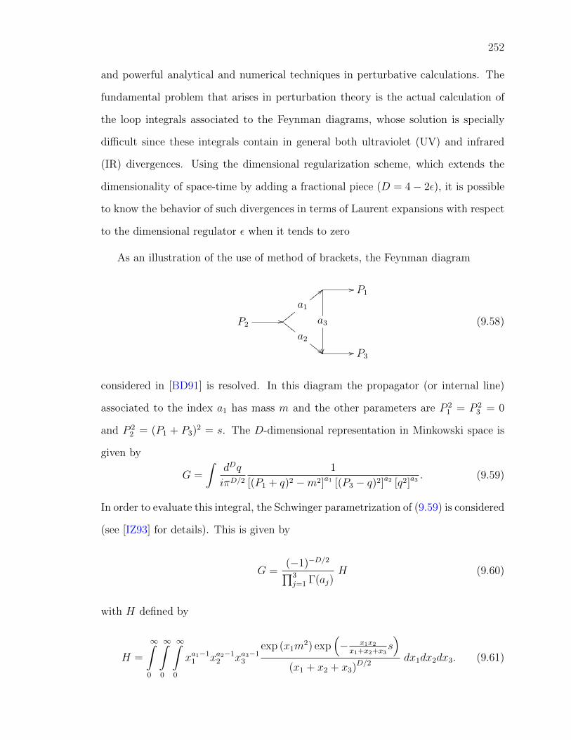
252
and powerful analytical and numerical techniques in perturbative calculations. The
fundamental problem that arises in perturbation theory is the actual calculation of
the loop integrals associated to the Feynman diagrams, whose solution is specially
difficult since these integrals contain in general both ultraviolet (UV) and infrared
(IR) divergences. Using the dimensional regularization scheme, which extends the
dimensionality of space-time by adding a fractional piece (D = 4− 2ε), it is possible
to know the behavior of such divergences in terms of Laurent expansions with respect
to the dimensional regulator ε when it tends to zero
As an illustration of the use of method of brackets, the Feynman diagram
P2
P1
P3
// a3
��
a1yyyy
<<yyyy//
a2
EEEE
""EEEE
//
(9.58)
considered in [BD91] is resolved. In this diagram the propagator (or internal line)
associated to the index a1 has mass m and the other parameters are P 21 = P 2
3 = 0
and P 22 = (P1 + P3)2 = s. The D-dimensional representation in Minkowski space is
given by
G =
∫dDq
iπD/21
[(P1 + q)2 −m2]a1 [(P3 − q)2]a2 [q2]a3. (9.59)
In order to evaluate this integral, the Schwinger parametrization of (9.59) is considered
(see [IZ93] for details). This is given by
G =(−1)−D/2∏3j=1 Γ(aj)
H (9.60)
with H defined by
H =
∞∫0
∞∫0
∞∫0
xa1−11 xa2−1
2 xa3−13
exp (x1m2) exp
(− x1x2x1+x2+x3
s)
(x1 + x2 + x3)D/2dx1dx2dx3. (9.61)
253
To apply the method of brackets the exponential terms are expanded as
exp(x1m
2)
exp
(− x1x2
x1 + x2 + x3
s
)=∑n1,n2
φn1,n2 (−1)n1m2n1sn2xn1+n2
1 xn22
(x1 + x2 + x3)n2,
and then (9.61) is transformed into
∑n1,n2
φn1,n2(−m2)n1sn2
∞∫0
∞∫0
∞∫0
xa1+n1+n2−11 xa2+n2−1
2 xa3−13
(x1 + x2 + x3)D/2+n2dx1dx2dx3. (9.62)
Further expanding
1
(x1 + x2 + x3)D/2+n2=
∑n3,n4,n5
φn3,n4,n5 xn31 x
n42 x
n53
⟨D2
+ n2 + n3 + n4 + n5
⟩Γ(D
2+ n2)
,
and replacing into (9.62) and substituting the resulting integrals by the corresponding
brackets yields
H =∑{n}
φ{n}(−1)n1m2n1sn2
⟨D2
+ n2 + n3 + n4 + n5
⟩Γ(D
2+ n2)
(9.63)
× 〈a1 + n1 + n2 + n3〉 〈a2 + n2 + n4〉 〈a3 + n5〉 .
This bracket series is now evaluated employing Rules 9.2.4 and 9.2.5. Possible choices
for free variables are n1, n2, and n4. The series associated to n2 converges for | sm2 | < 1,
whereas the series associated to n1, n4 converge for |m2
s| < 1. The following two
representations for G follow from here.
Theorem 9.6.1. In the region | sm2 | < 1,
H = η2 · 2F1
(a1 + a2 + a3 − D
2, a2
D2
∣∣∣∣ sm2
)(9.64)

254
with η2 defined by
η2 =(−m2
)D2−a1−a2−a3 Γ(a2)Γ(a3)Γ
(a1 + a2 + a3 − D
2
)Γ(D2− a2 − a3
)Γ(D2
) .
Theorem 9.6.2. In the region |m2
s| < 1,
H = η1 · 2F1
(a1 + a2 + a3 − D
2, 1 + a1 + a2 + a3 −D
1 + a1 + a3 − D2
∣∣∣∣m2
s
)(9.65)
+ η4 · 2F1
(1 + a2 − D
2, a2
1− a1 − a3 + D2
∣∣∣∣m2
s
)
with η1, η4 defined by
η1 = sD2−a1−a2−a3 Γ(a3)Γ
(a1 + a2 + a3 − D
2
)Γ(D2− a1 − a3
)Γ(D2− a2 − a3
)Γ (D − a1 − a2 − a3)
,
η4 = s−a2(−m2
)D2−a1−a3 Γ(a2)Γ(a3)Γ
(a1 + a3 − D
2
)Γ(D2− a2 − a3
)Γ(D2− a2
) .
These two solutions are now specialized to a1 = a2 = a3 = 1. This situation is
specially relevant, since when an arbitrary Feynman diagram is computed, the indices
associated to the propagators are normally 1. Then, with D = 4− 2ε, the equations
(9.64) and (9.65) take the form
H = (−m2)−1−εΓ(ε− 1)2F1
(1 + ε, 1
2− ε
∣∣∣∣ sm2
)(9.66)
for | sm2 | < 1, as well as
H = s−1−εΓ(−ε)2Γ(1 + ε)
Γ(1− 2ε)
(1− m2
s
)−2ε
−m−2εΓ(ε)
εs2F1
(ε, 1
1− ε
∣∣∣∣m2
s
)(9.67)
for |m2
s| < 1. Observe that these representations both have a pole at ε = 0 of first
order (for the second representation, each of the summands has a pole of second order

255
which cancel each other).
9.7 Conclusions and future work
The method of brackets provides a very effective procedure to evaluate definite
integrals over the interval [0,∞). The method is based on a heuristic list of rules on
the bracket series associated to such integrals. In particular, a variety of examples
that illustrate the power of this method has been provided. A rigorous validation of
these rules as well as a systematic study of integrals from Feynman diagrams is in
progress.

256
Chapter 10
A fast numerical algorithm for theintegration of rational functions
The contents of this chapter (apart from minor corrections or adaptions) have
been published as:
[MMMS10] A fast numerical algorithm for the integration of rational functions(with Dante Manna, Luis Medina, Victor H. Moll)
published in Numerische Mathematik, Vol. 115, Nr. 2, Apr 2010, p. 289-307
Abstract A new iterative method for high-precision numerical integration of ra-
tional functions on the real line is presented. The algorithm transforms the rational
integrand into a new rational function preserving the integral on the line. The coeffi-
cients of the new function are explicit polynomials in the original ones. These trans-
formations depend on the degree of the input and the desired order of the method.
Both parameters are arbitrary. The formulas can be precomputed. Iteration yields
an approximation of the desired integral with m-th order convergence. Examples
illustrating the automatic generation of these formulas and the numerical behaviour
of this method are given.

257
10.1 Introduction
The numerical integration of the elliptic integral
G(a, b) =
∫ π/2
0
dθ√a2 cos2 θ + b2 sin2 θ
(10.1)
can be accomplished by iterating the transformation
Le : R2 → R2, (a, b) 7→(a+ b
2,√ab
). (10.2)
Gauss [Gau99] established that G(a, b) is invariant under the transformation Le, i.e.,
G(Le(a, b)) = G(a, b). (10.3)
Moreover, the iterates (an, bn) defined recursively by (a0, b0) = (a, b) and (an, bn) =
Le(an−1, bn−1) for n ≥ 1, satisfy
|an+1 − bn+1| ≤1
2|an − bn|2, (10.4)
illustrating the quadratic convergence of an and bn to a common limit AGM(a, b).
This is the arithmetic-geometric mean of a and b. Le is known as the elliptic Landen
transformation. The reader will find in [MM08a] a survey of the diverse aspects of
this transformation and its generalizations.
The invariance of the integral G(a, b) under Le yields
G(a, b) =π
2AGM−1(a, b). (10.5)
In particular, the value of the elliptic integral G(a, b) can be approximated using
the iterates an (or bn). The functions G(a, b) and AGM(a, b) along with the formula

258
(10.5), are at the center of highly effective computation of the basic constants of
Analysis [BB98].
A scheme for the computation of the rational integral
F (a, b) =
∫ ∞−∞
b0xp−2 + . . .+ bp−3x+ bp−2
a0xp + . . .+ ap−1x+ apdx, (10.6)
with a = (a0, a1, . . . , ap), b = (b0, b1, . . . , bp−2), is presented here. Rational Landen
transformations
Lm,p : C2p → C2p, (a, b) 7→ Lm,p(a, b) (10.7)
which preserve the integral F (a, b) are constructed. Iteration of Lm,p yields a sequence
of coefficients (an,0, an,1, · · · , an,p) and (bn,0, bn,1, · · · , bn,p−2) for a sequence of rational
functions which are shown to converge to a constant multiple of 1/(x2 + 1). The
invariance of the integral F (a, b) under Lm,p yields
F (a, b) = c
∫ ∞−∞
dx
x2 + 1= πc = π lim
n→∞
bn,0an,0
, (10.8)
that determines the constant c. The sequence {πbn,0/an,0 : n = 1, 2, 3 . . .} of approx-
imations to the integral F (a, b) converges with order m; that is, the error en :=
|πbn,0/an,0 − F (a, b)| satisfies
|en+1 − en| ≤ C|en − en−1|m (10.9)
with an absolute constant C.
The outlined algorithm for computing rational integrals over the real line, pre-
sented in more detail in Section 10.6, consists of the two parts:
• Creation of the rational Landen transformation Lm,p where m is the desired
order of convergence and p is the degree of the denominator of the rational

259
function to be integrated. This is discussed in Section 10.2.
• Iteration of the Landen transformation, which is analyzed in Sections 10.3 and
10.6 with the view towards complexity and implementation, respectively.
Numerical examples of this method are discussed in Section 10.4.
Remark 10.1.1. Given m and p, the map Lm,p can be precomputed and the result
can be stored for use in the second part of the algorithm. Therefore, the first part
of the algorithm carries a one-time cost and is not figured into the complexity of the
method which is discussed in Section 10.3.
Remark 10.1.2. The numerical method for the integration of rational functions
presented here is different in spirit than the standard ones: the approximation to the
integral is obtained from a recurrence acting on the coefficients of the integrand. In
particular, the domain of integration is not discretized and the integrand is never
evaluated. Examples that illustrate the method and a study of the cost involved are
presented.
Future work. The algorithm presented here is restricted to integrals on the whole
line. The extension to a finite interval requires the development of Landen transfor-
mations on the half line. This question is open, even for the simplest case of
I2(a, b, c) :=
∫ ∞0
dx
ax2 + bx+ c. (10.10)
The method has been coupled with Pade approximations [BCGK+10] to produce
a fast, robust integration algorithm for some non-rational integrands; namely, those
of the form R(µ(x))µ′(x) for a rational function R and an increasing change of scale
µ. Extensions to all smooth integrands remain to be completed.
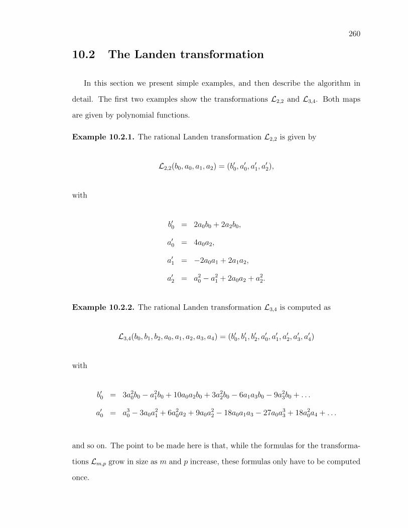
260
10.2 The Landen transformation
In this section we present simple examples, and then describe the algorithm in
detail. The first two examples show the transformations L2,2 and L3,4. Both maps
are given by polynomial functions.
Example 10.2.1. The rational Landen transformation L2,2 is given by
L2,2(b0, a0, a1, a2) = (b′0, a′0, a′1, a′2),
with
b′0 = 2a0b0 + 2a2b0,
a′0 = 4a0a2,
a′1 = −2a0a1 + 2a1a2,
a′2 = a20 − a2
1 + 2a0a2 + a22.
Example 10.2.2. The rational Landen transformation L3,4 is computed as
L3,4(b0, b1, b2, a0, a1, a2, a3, a4) = (b′0, b′1, b′2, a′0, a′1, a′2, a′3, a′4)
with
b′0 = 3a20b0 − a2
1b0 + 10a0a2b0 + 3a22b0 − 6a1a3b0 − 9a2
3b0 + . . .
a′0 = a30 − 3a0a
21 + 6a2
0a2 + 9a0a22 − 18a0a1a3 − 27a0a
33 + 18a2
0a4 + . . .
and so on. The point to be made here is that, while the formulas for the transforma-
tions Lm,p grow in size as m and p increase, these formulas only have to be computed
once.
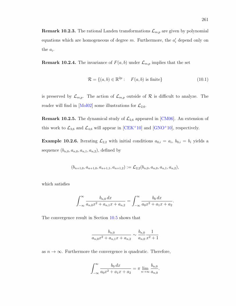
261
Remark 10.2.3. The rational Landen transformations Lm,p are given by polynomial
equations which are homogeneous of degree m. Furthermore, the a′i depend only on
the ai.
Remark 10.2.4. The invariance of F (a, b) under Lm,p implies that the set
R = {(a, b) ∈ R2p : F (a, b) is finite} (10.1)
is preserved by Lm,p. The action of Lm,p outside of R is difficult to analyze. The
reader will find in [Mol02] some illustrations for L2,6.
Remark 10.2.5. The dynamical study of L2,6 appeared in [CM06]. An extension of
this work to L3,6 and L4,6 will appear in [CEK+10] and [GNO+10], respectively.
Example 10.2.6. Iterating L2,2 with initial conditions a0,i = ai, b0,i = bi yields a
sequence (bn,0, an,0, an,1, an,2), defined by
(bn+1,0, an+1,0, an+1,1, an+1,2) := L2,2(bn,0, an,0, an,1, an,2),
which satisfies
∫ ∞−∞
bn,0 dx
an,0x2 + an,1x+ an,2=
∫ ∞−∞
b0 dx
a0x2 + a1x+ a2
.
The convergence result in Section 10.5 shows that
bn,0an,0x2 + an,1x+ an,2
∼ bn,0an,0
1
x2 + 1
as n→∞. Furthermore the convergence is quadratic. Therefore,
∫ ∞−∞
b0 dx
a0x2 + a1x+ a2
= π limn→∞
bn,0an,0
.
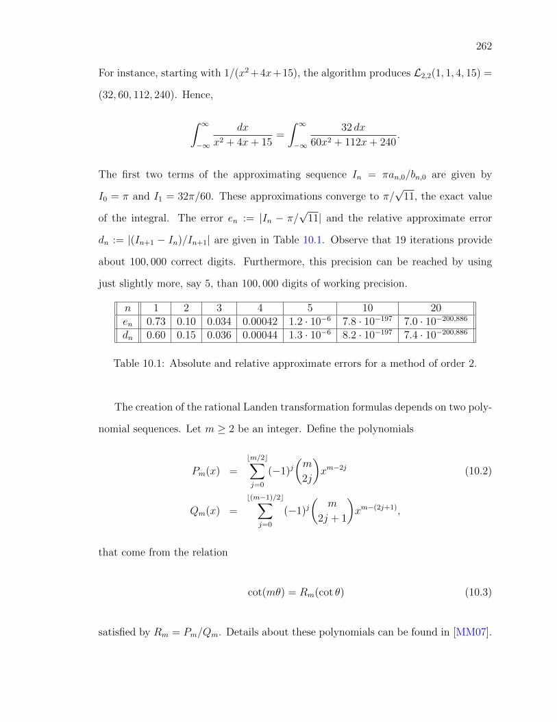
262
For instance, starting with 1/(x2 +4x+15), the algorithm produces L2,2(1, 1, 4, 15) =
(32, 60, 112, 240). Hence,
∫ ∞−∞
dx
x2 + 4x+ 15=
∫ ∞−∞
32 dx
60x2 + 112x+ 240.
The first two terms of the approximating sequence In = πan,0/bn,0 are given by
I0 = π and I1 = 32π/60. These approximations converge to π/√
11, the exact value
of the integral. The error en := |In − π/√
11| and the relative approximate error
dn := |(In+1 − In)/In+1| are given in Table 10.1. Observe that 19 iterations provide
about 100, 000 correct digits. Furthermore, this precision can be reached by using
just slightly more, say 5, than 100, 000 digits of working precision.
n 1 2 3 4 5 10 20en 0.73 0.10 0.034 0.00042 1.2 · 10−6 7.8 · 10−197 7.0 · 10−200,886
dn 0.60 0.15 0.036 0.00044 1.3 · 10−6 8.2 · 10−197 7.4 · 10−200,886
Table 10.1: Absolute and relative approximate errors for a method of order 2.
The creation of the rational Landen transformation formulas depends on two poly-
nomial sequences. Let m ≥ 2 be an integer. Define the polynomials
Pm(x) =
bm/2c∑j=0
(−1)j(m
2j
)xm−2j (10.2)
Qm(x) =
b(m−1)/2c∑j=0
(−1)j(
m
2j + 1
)xm−(2j+1),
that come from the relation
cot(mθ) = Rm(cot θ) (10.3)
satisfied by Rm = Pm/Qm. Details about these polynomials can be found in [MM07].

263
Let A, B be polynomials. The change of variables y = Rm(x) yields a new pair
of polynomials A1, B1 such that
∫ ∞−∞
B1(x)
A1(x)dx =
∫ ∞−∞
B(x)
A(x)dx. (10.4)
The change of variables requires the domain to be splitted according to the branches
of the inverse R−1m . These are specified by the intervals (qj−1, qj) where q0 = −∞,
qj = cot(πj/m) for 1 ≤ j ≤ m − 1, and qm = +∞. The function y = Rm(x) is
invertible on each of the subintervals (qj−1, qj), and the (local) inverse is denoted by
x = ωj(y). After substituting y = Rm(x) in each interval, it follows that
∫ ∞−∞
B(x)
A(x)dx =
m∑j=1
∫ qj
qj−1
B(x)
A(x)dx =
∫ ∞−∞
m∑j=1
B(ωj(y))
A(ωj(y))ω′j(y)dy. (10.5)
The integrand on the right-hand side of (10.5) is indeed a rational function B1/A1;
see [MM07]. The rational Landen transformation Lm : C(x) → C(x) is defined by
B/A 7→ B1/A1. The full details are given below.
Step 1 The rational function Rm = Pm/Qm comes from (10.2). First construct the
polynomial
A1(x) := Res (A,Pm − xQm)
where Res denotes the resultant. The degrees of the polynomials involved are
p := degA and m = deg(Pm − xQm), respectively. The degree of the de-
nominator is preserved; that is, deg(A1) = deg(A). The coefficients of A1 are
polynomials in those of A.
Step 2 The polynomial Em(x) := [Pm(x)]pA1(Rm(x)) is a multiple of A. Compute
the quotient
C(x) := E(x)B(x)
A(x)=
s∑k=0
ckxs−k,
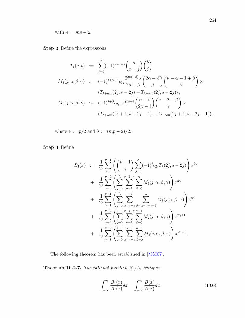
264
with s := mp− 2.
Step 3 Define the expressions
Tx(a, b) :=x∑j=0
(−1)a−x+j
(a
x− j
)(b
j
),
M1(j, α, β, γ) := (−1)j+α−βc2j22(α−β)α
2α− β
(2α− ββ
)(ν − α− 1 + β
γ
)×
(Tλ+αm(2j, s− 2j) + Tλ−αm(2j, s− 2j)) ,
M2(j, α, β, γ) := (−1)j+βc2j+122β+1
(α + β
2β + 1
)(ν − 2− β
γ
)×
(Tλ+αm(2j + 1, s− 2j − 1)− Tλ−αm(2j + 1, s− 2j − 1)) ,
where ν := p/2 and λ := (mp− 2)/2.
Step 4 Define
B1(x) :=1
2s
ν−1∑γ=0
((ν − 1
γ
) λ∑j=0
(−1)jc2jTλ(2j, s− 2j)
)x2γ
+1
2s
ν−2∑γ=0
(λ∑j=0
ν−1−γ∑α=1
α∑β=0
M1(j, α, β, γ)
)x2γ
+1
2s
ν−1∑γ=1
(λ∑j=0
ν−1∑α=ν−γ
α∑β=α−ν+γ+1
M1(j, α, β, γ)
)x2γ
+1
2s
ν−2∑γ=0
(λ−1∑j=0
ν−1−γ∑α=1
α−1∑β=0
M2(j, α, β, γ)
)x2γ+1
+1
2s
ν−2∑γ=1
(λ−1∑j=0
ν−1∑α=ν−γ
α−1∑β=0
M2(j, α, β, γ)
)x2γ+1.
The following theorem has been established in [MM07].
Theorem 10.2.7. The rational function B1/A1 satisfies
∫ ∞−∞
B1(x)
A1(x)dx =
∫ ∞−∞
B(x)
A(x)dx (10.6)

265
whenever one of the integrals is finite. Moreover degA1 = degA.
Definition 10.2.8. The rational Landen transformation Lm : C(x)→ C(x) is defined
by Lm(B/A) = B1/A1. When Lm is acting on the coefficients of a rational function of
degree p we write Lm,p(b0, b1, . . . , bp−2, a0, a1, . . . , ap) as in (10.7) and Example 10.2.6.
Precomputed formulas for the Lm,p as well as a program written in Mathematica
that generates these formulas following the above algorithm and featuring the numer-
ical integration of rational functions over the real line, as outlined in the introduction,
are available for download from the authors. Some details of the implementation will
be discussed in Section 10.6.
10.3 Complexity of the algorithm
This section discusses the complexity of computing definite integrals using Landen
transformations. The analysis is restricted to the cost of one iteration. The actual
generation of the Landen transformation is not considered since it is a one-time cost.
Examples 10.2.1 and 10.2.2 illustrate the fact that Lm,p is a mapping C2p → C2p
defined by polynomial equations with integer coefficients. Assume that these polyno-
mial equations appear in expanded form. The number of multiplications cm,p involved
in computing Lm,p not including multiplications with constants is now counted. Ad-
ditions and multiplying with constants have lower complexity than multiplication
which is why they are not included in this count.

266
Example 10.3.1. Example 10.2.1 gives L2,2(b0, a0, a1, a2) = (b′0, a′0, a′1, a′2) with
b′0 = 2a0b0 + 2a2b0,
a′0 = 4a0a2,
a′1 = −2a0a1 + 2a1a2,
a′2 = a20 − a2
1 + 2a0a2 + a22.
Hence L2,2 requires c2,2 = 9 multiplications. More values cm,p are given in Table 10.2.
p\m 2 3 4 52 9 32 75 1444 36 204 702 18966 94 756 3492 120408 195 2056 11895 4971210 351 4600 31923 15651212 574 9012 72858 409688
Table 10.2: Number of operations involved in Lm,p.
The data above suggest that cm,p = O(pm+1). Moreover, for m = 2 and m = 3
the number of multiplications cm,2p seem to be exactly
c2,2p =1
2(p+ 1)
(2 + 3p+ 4p2
), (10.1)
c3,2p =2
3p(15 + 13p+ 12p2 + 8p3
). (10.2)
Remark 10.3.2. As noted in Remark 10.2.3, the Landen transformation Lm,p only
involves monomials of degree m. Therefore, cm,p is the number of these monomials
times m−1. Writing the polynomial expressions defining Lm,p in a different form, one
may hope to decrease the cost of its computation. Experiments conducted in Math-
ematica show that writing these polynomials in multivariate Horner form decreases
the order of growth to O(pm).

267
Remark 10.3.3. From a practical point of view, the Landen transformations of order
2 are generally preferable to higher order ones. This is because combining n Landen
iterations L2,p into one step gives a method of order 2n (in fact, Ln2,p = L2n,p) which
requires nc2,p multiplications. Multiple experiments show that nc2,p � c2n,p.
10.4 Some numerical examples
In this section two examples that illustrate the procedure described in this work
are presented.
Example 10.4.1. This first example illustrates the behavior on highly oscillatory
integrands which, as it turns out, is basically no different from the behaviour on more
regular integrands. A Landen transformation of order 2 is applied to the rational
function
fk(x) =2kPk(x/2)(kbk/2c
)(x2k + 1)
, (10.1)
where Pk is the Legendre polynomial. The normalization factor is chosen so that
|fk(0)| = 1 for even k.
-1.0 -0.5 0.5 1.0
-1.0
-0.5
0.5
1.0
Figure 10.1: The oscillatory rational function f50(x)
The number of steps nk(d) needed for the relative error to drop below 10−d is
tabulated in Table 10.3. These calculations only require a working precision of a few
more, say 5, than d digits. Observe that, as expected, to obtain the 10 fold precision
only about log(2, 10) ≈ 3.32 additional iterations are necessary.

268
k 2 4 6 8 10 20 30 40 50nk(20) 6 7 8 8 9 10 10 11 11nk(50) 8 9 9 10 10 11 12 12 12nk(100) 9 10 10 11 11 12 13 13 13nk(1000) 12 13 14 14 14 15 16 16 17nk(10000) 15 16 17 17 18 19 19 20 20
Table 10.3: Number of steps nk(d) needed to get relative error less than 10−d.
Example 10.4.2. The method proposed here is also applicable to problems that are
nearly singular, that is, to rational functions with poles arbitrarily close to the real
axis. For fixed ε > 0, apply L2,2 to the rational function
fε(x) =1
(x− 1)2 + ε2=
1
x2 − 2x+ (1 + ε2)(10.2)
which over the real line integrates to 1/ε. For decreasing values of ε = 10−k the
number of steps nk(d) needed so that the relative error is less than 10−d can be found
in Table 10.4. In this case, it is sufficient to use a working precision of d + 2k. The
data in Table 10.4 suggest that the number of steps nk(d) grows linear in k and, as
expected, logarithmic in d.
k 1 2 3 4 5 10 20 40nk(20) 9 13 16 19 23 39 72 139nk(50) 11 14 17 21 24 41 74 140nk(100) 12 15 18 22 25 42 75 141nk(1000) 15 18 22 25 28 45 78 145nk(10000) 18 22 25 28 32 48 81 148
Table 10.4: Number of steps nk(d) needed to get relative error less than 10−d whenintegrating f10−k .

269
10.5 Convergence of Landen iterates
In this section the convergence of the iterates of the Landen transformation Lm,pstarting at the rational function
f(x) =B(x)
A(x)=b0x
p−2 + . . .+ bp−3x+ bp−2
a0xp + . . .+ ap−1x+ ap
is considered. Denote by fn = Bn/An the Landen iterates Lnm,p(f). Assuming that f
has no poles on the real line, Theorem 10.5.7 shows that, as n→∞,
fn →c
x2 + 1, (10.1)
where c is determined by the integral of f (and vice versa). Moreover, convergence is
of order m. This implies the convergence of the coefficients of An = an,0xp+an,1x
p−1+
. . . + an,p and Bn = bn,0xp−2 + bn,1x
p−3 + . . . + bn,p−2 as described in the following
proposition.
Proposition 10.5.1. Let λ+ be the number of roots of A with positive imaginary part
and λ− the number of roots with negative imaginary part (note that λ+ + λ− is the
degree of A). Then for the constant c defined in (10.1)
Bn
an,0→ c(x− i)λ+−1(x+ i)λ−−1,
Anan,0→ (x− i)λ+(x+ i)λ− .
Note that the constant c in (10.1) vanishes if either λ+ = 0 or λ− = 0.
Proof. The proof is given for m = 2, the general case can be established by similar
methods. Recall that the denominator An only depends on A and it is transformed
according to
An+1(x) = Resz(An(z), z2 − 2xz − 1). (10.2)

270
Hence, if An/an,0 =∏
k(x− λn,k) then
An+1/an,0 =∏k
(λ2n,k − 2λn,kx− 1
).
Therefore the roots of An+1(x) are λn+1,k =λ2n,k−1
2λn,k. Note that
Im
(λ2 − 1
2λ
)=
1
2
(1 +
1
|λ|2)
Im(λ),
which implies that the signs of the imaginary part of the roots of A are preserved
by the Landen iterations. In particular, this shows that the integrablity of a rational
function is preserved by Lm,p.
The transformation λ 7→ λ2 − 1
2λ= λ − λ2 + 1
2λis the Newton map of λ2 + 1.
Therefore, each root λn,k converges to i or −i depending on the sign of Im λ1,k.
Furthermore, the Newton map is known to exhibit quadratic convergence. This es-
tablishes the result about An. Theorem 10.5.7 shows that Bn/An → c/(x2 + 1). This
gives the corresponding result for Bn.
Corollary 10.5.2. If A has only real coefficients, then p is even and
Bn
an,0→ c(x2 + 1)p/2−1,
Anan,0→ (x2 + 1)p/2.
Remark 10.5.3. An explicit and curious formula for the denominator A1 of L2(1/A)
is described next. This is an expression independent of the roots of A. In the compu-
tation of A1(x) = Resz(A(z), z2 − 2xz − 1), reduce A(z) modulo z2 − 2xz − 1 before
computing the resultant. Proceeding in a recursive manner, write zn ≡ an(x)+bn(x)z.
Then z2 ≡ 1 + 2xz leads to the recurrence
an+1(x) = bn(x), bn+1(x) = an(x) + 2xbn(x).

271
Therefore zn ≡ bn−1(x) + bn(x)z where bn(x) is defined by
bn+1(x) = 2xbn(x) + bn−1(x), b0 = 0, b1 = 1. (10.3)
It follows that zn ≡ Fn−1(2x)+Fn(2x)z where Fn(x) is the nth Fibonacci polynomial.
These polynomials are defined recursively by F0(x) = 0, F1(x) = 1 and Fn+1(x) =
xFn(x) + Fn−1(x) and they are explicitely given by
Fn+1(x) =
bn/2c∑k=0
(n− kk
)xn−2k.
If A(z) =∑akz
k then A(z) ≡ a(x) + b(x)z for a(x) =∑akFk−1(2x) and b(x) =∑
akFk(2x). It follows that
A1(x) = a(x)2 − b(x)2 + 2a(x)b(x)x
= a(x)(a(x) + 2xb(x))− b(x)2
=(∑
akFk−1
)(∑akFk+1
)−(∑
akFk
)2
where Fk is used to abbreviate Fk(2x).
Remark 10.5.4. The proof of Proposition 10.5.1 contains explicitly the transforma-
tion of the denominator under the Landen transformation L2 in terms of its roots. In
particular,
L2
(1
x− λ
)=
−2λ
−2λx+ λ2 − 1=
1
x− λ2−12λ
.
For a rational function f = B/A, with no repeated poles off the real line and
deg(B) ≤ deg(A) − 2 (for integrability), consider the partial fraction decomposition
f =∑
k bk/(x− λk). Then, by linearity of L2,
L2(f) = L2
(∑k
bkx− λk
)=∑k
bk
x− λ2k−1
2λk
.

272
Assume that the poles of Ln2 (f) remain simple. Then
Ln2f →∑k
bkx− λ∞,k
where λ∞,k is either i or −i depending on the sign of Im λk. Thus, for some constants
c±,
Ln2f →c+
x− i +c−x+ i
=c
x2 + 1,
where the last equality follows from Theorem 10.2.7 and the fact that a Landen
transformation preserves integrability.
The general proof requires some machinery from complex analysis. To this end,
identify the integral of the rational function f = B/A over the real line with the
integral of the holomorphic 1-form φ = f(z)dz over the real projective line RP 1; that
is, ∫ ∞−∞
f(x)dx =
∫RP 1
φ,
where RP 1 is the completed real axis sitting inside the Riemann sphere CP 1. Recall
that f being a rational function corresponds to a holomorphic function on CP 1.
The next required concept is that of a pull-back of a holomorphic 1-form. After
the definition, recall the change of variables formula that connects the integral of a
1-form to that of its pull-back. The reader will find all these concepts in [Sha94].
Definition 10.5.5. Let φ be a 1-form on a Riemann surface S, and π : S → T a
holomorphic mapping between Riemann surfaces. The pull-back of φ induced by π is
defined as
π∗φ|U =k∑i=1
σ∗i φ,
on all U ⊂ T simply connected and containing no critical values of π. Here σ1, ..., σk :
U → S are the distinct sections of π.

273
It is an elementary consequence of this definition that for holomorphic mappings
π1 : S2 7→ S3 and π2 : S1 7→ S2,
π1∗π2∗φ = (π1 ◦ π2)∗φ
for any 1-form φ on S1. The next lemma concerning holomorphic pull-backs and their
path integrals is again an immediate consequence of the definition.
Lemma 10.5.6. If π : S → T is a holomorphism of Riemann surfaces, and φ is a
holomorphic 1-form on S, then π∗φ is a holomorphic 1-form on T . Furthermore, for
any oriented rectifiable curve γ on T , the identity
∫γ
π∗φ =
∫π−1γ
φ (10.4)
holds.
Let f = B/A be a rational function. The pull-back of the 1-form φ = f(z)dz on
CP 1 induced by Rm : CP 1 → CP 1 is the 1-form
(Rm)∗φ =m∑j=1
B(ωj(y))
A(ωj(y))ω′j(y)dy.
Note that the right-hand side of (10.5) is precisely the integral of (Rm)∗φ over the
projective real line. In this case, Lemma 10.5.6 amounts to (10.5). The map Lm may
therefore be identified with (Rm)∗. The following is a restatement of (10.1).
Theorem 10.5.7. Let φ be a holomorphic 1-form in a neighborhood U of RP 1 ⊂ CP 1.
Then
limn→∞
(Rm)n∗φ =1
π
(∫RP 1
φ
)dz
z2 + 1
where the convergence is of order m and uniform on compact subsets of U .
274
Remark 10.5.8. Let f = B/A be a rational function such that its integral over the
real line is finite. Then the 1-form f(z)dz on CP 1 is holomorphic on some open set
U ⊃ RP 1. In particular, for β = min{| Im x| : A(x) = 0}, and N = max{|x| : A(x) =
0}, f(z)dz is holomorphic on
Vε = {x ∈ CP 1 : | Im x| < β − ε} ∪ {x ∈ CP 1 : |x| > N + ε}
for all ε < β.
A statement equivalent to Theorem 10.5.7 is proved now. This follows from con-
jugation by the map M(z) = z+iz−i . Recall that Rm = M−1 ◦ fm ◦M , see for instance
[MM07], where fm(z) = zm, so that Rnm = M−1 ◦ fnm ◦M and therefore
limn→∞
(Rm∗)nφ = M−1
∗ limn→∞
(fm∗)nφ1
where φ1 = M∗φ. On the other hand, one verifies that
M∗dz
z2 + 1= − dz
2iz.
Finally, observe that, by Lemma 10.5.6,
∫RP 1
φ =
∫RP 1
M−1∗ φ1 = −
∫S1
φ1
where S1 denotes the path that rotates once around the unit circle in counterclockwise
direction. Theorem 10.5.7 is therefore equivalent to the following statement.
Theorem 10.5.9. Let φ be a holomorphic 1-form in a neighborhood U of S1. Then
limn→∞
(fm)n∗φ =1
2πi
(∫S1
φ
)dz
z

275
where the convergence is of order m and uniform on compact subsets of U .
Proof. Using the local coordinate z, write φ = φ(z)dz where φ(z) is analytic on an
annulus 1R< |z| < R for some R > 1. The function φ(z) admits a Laurent expansion
φ(z) =∞∑
k=−∞
akzk
and the coefficients ak satisfy
‖φ‖ :=∞∑
k=−∞
|ak|R|k| <∞.
Since
a−1 =1
2πi
∫S1
φ(z)dz
it is required to show that
limn→∞
(fm)n∗ φ = a−1dz
z.
In order to verify this, start with
(fm)∗φ =m∑j=1
σ∗j (φ(z)dz) =∞∑
k=−∞
m∑j=1
akσ∗j (z
kdz) =∞∑
k=−∞
ak(fm)∗(zkdz)
where σ1(w), ..., σm(w) are the m-th root sections of w = fm(z) = zm, defined by
σj(w) = e2πij/mσ0(w)
where σ0(w) = w1/m is the value of the complex m-th root whose argument is between

276
0 and 2π/m. A direct calculation yields
(fm)∗(zkdz) =
m∑j=1
σ∗j (zkdz)
=m∑j=1
e2πijk/mwk/m(
1
me2πij/mw1/m−1
)dw
=1
m
(m∑j=1
e2πij(k+1)/m
)w(k+1−m)/mdw
=
z(k+1−m)/mdz if m|k + 1,
0 if m|k + 1.
This establishes the formula
(fm)∗φ =∞∑
k=−∞
am(k+1)−1zkdz.
Consequently,
∥∥∥∥(fm)n∗φ− a−1dz
z
∥∥∥∥ =
∥∥∥∥∥∞∑
k=−∞
amn(k+1)−1zkdz − a−1
dz
z
∥∥∥∥∥=
∞∑k=−∞,k 6=−1
|amn(k+1)−1|R|k|
=∞∑
k=−∞,k 6=−1
|amn(k+1)−1|R|mn(k+1)−1| R|k|
R|mn(k+1)−1|
≤ R
Rmn
∞∑k=−∞,k 6=−1
|amn(k+1)−1|R|mn(k+1)−1|
≤ R
Rmn
∥∥∥∥φ− a−1dz
z
∥∥∥∥ .As n→∞, this quantity converges to zero to order m.

277
Corollary 10.5.10. For a rational function f
∫ ∞−∞
f(x)dx = π limn→∞
Lnm(f)(0)
provided that the integral is finite. In that case, convergence is of order m.
10.6 Implementation
In this section the implementation of the numerical scheme proposed in the pre-
vious sections is discussed. Assume that A and B are polynomials and let
I :=
∫ ∞−∞
B(x)
A(x)dx. (10.1)
The first issue under consideration is that the exact evaluation of the iterates of
Lnm,p(B/A) usually leads to extreme growth in the size of the coefficients. Therefore,
while computing these iterates numerically, the coefficients are normalized after each
iteration by keeping the denominator polynomial with leading coefficient 1.
Example 10.6.1. This continues Example 10.2.6 where
∫ ∞−∞
dx
x2 + 4x+ 15=
π√11
is approximated using L2,2. The first iterate is 3260x2+112x+240
. The next two Landen
iterates are
19200
57600x2 + 40320x+ 77456,
5186150400
17845862400x2 + 1601187840x+ 16614420736.
Experiments show that the number of digits in the coefficients grows exponentially
even if common factors are cancelled.
278
Fix m ∈ N and let p = deg(A). The normalization proceeds as follows: let
b0 = (b0,0, b0,1, . . . , b0,p−2) and a0 = (a0,0, a0,1, . . . , a0,p) (10.2)
be the coefficients of the initial rational function B/A. For n ≥ 1, let
(bn, an) =1
a′n,0(b′n, a
′n), where (b′n, a
′n) = Lm,p(bn−1, an−1). (10.3)
Recall that the rational Landen transformations preserve the degree of the denomina-
tor. Hence, a′n,0 6= 0 throughout. If the integral of B/A converges, then by Corollary
10.5.10 its value is given by π limn→∞ bn,0.
Proposition 10.5.1 shows that, if the integral over B/A is finite, then an converges
to the coefficients ck of one of the p+ 1 candidates
(x− i)k(x+ i)p−k, 0 ≤ k ≤ p, (10.4)
depending on the number k of roots of A with positive imaginary part. In particular,
Corollary 10.5.2 shows that if all coefficients are real, then an will converge to
((p/2
0
), 0,
(p/2
1
), 0, . . . ,
(p/2
p/2− 1
), 0,
(p/2
p/2
)). (10.5)
Conversely, if convergence to one of the candidates in (10.4) is observed, then
the invariance of the integral under Lm shows that the initial integral must be finite.
Thus the algorithm also detects the integrability of rational functions.
After each step, the implementation checks if the approximate relative error |(bn,0−
bn−1,0)/bn,0| is less than the precision goal. The distance of the coefficients an to their
limiting values is also monitored. While computations may be made symbolically
(provided that the initial coefficients are known exactly) it is generally sensible to

279
work with a fixed precision throughout. For most integrands (compare Examples
10.2.6 and 10.4.1) this working precision need only be slightly larger, say 5 digits, than
the precision goal. In case of almost singular integrands (compare Example 10.4.2)
the working precision may need to be chosen somewhat higher. For the problems
considered by the authors, a reasonable choice (currently used as a default in the
Mathematica implementation mentioned below) seems to be 20 additional digits.
The implementation of the Landen iteration method is given below in pseudo code.
Input: the coefficients (b0, a0) of the rational function B/A of degree p, the order m
of the method, and the precision goal ε > 0.
Output: an approximation (produced using Landen iterations of order m) to the
integral of B/A over the real line with (approximate) relative error less than ε.
n := 0
repeat
n := n+ 1
(b′n, a′n) := Lm,p(bn−1, an−1)
(bn, an) := 1a′n,0
(b′n, a′n)
until |(bn,0 − bn−1,0)/bn,0| < ε and |(an,j − ck,j)/ck,j| < ε
for all j and some 0 ≤ k ≤ p
OUTPUT πbn,0
The described method for integrating rational functions over the real line has been
implemented in Mathematica and can be downloaded from the website
http://www.math.tulane.edu/∼vhm
The Landen transformations can be either generated by the package, following the
description in Section 10.2, or downloaded as well. The following examples demon-

280
strate the basic usage of this package. Further examples can be obtained from the
above website.
Example 10.6.2. Given a rational function f , its integral over the entire real line
can be computed using the function NLandenIntegrate. For instance, to compute
the integral of 1/(x2 + 4x+ 15) to a precision of 100 digits, input:
NLandenIntegrate[1/(x^2+4x+15), PrecisionGoal->100]
> 0.94722582509948293642963438181697406661998807...
By default the Landen transformation is chosen to be of order 2 (see Remark 10.3.3 for
why this is desirable) but higher orders m may be used by setting MethodOrder->m.
Further options exist to control the number of iterations, set the working precision
manually, or to obtain the intermediate Landen iterates.
Example 10.6.3. Before using the function NLandenIntegrate demonstrated in the
previous example the corresponding Landen transformation needs to be available.
The command
GenerateLandenTransforms[10]
will generate the Landen transformations of order 2 for degrees up to 10. Note that
on a modern desktop computer this will take less than half a second. After execution,
the Landen transformations are directly available as follows, compare example 10.2.1:
LandenStep[{{b0}, {a0,a1,a2}}, 2]
> {{2a0b0+2a2b0}, {4a0a2, -2a0a1+2a1a2, a0^2-a1^2+2a0a2+a2^2}}
Again, higher orders than 2 can be generated using the option MethodOrder. Once
generated, these Landen transformations may be stored to a file. Alternatively, pre-
generated Landen transformations are available for download.

281
10.7 Conclusions
A numerical method for the integration of rational functions on the real line has
been described. The method has order of convergence prescribed by the user. Its
convergence and robustness have been analyzed. Examples illustrating speed of con-
vergence as well as the flexibility of this method have been provided. A Mathematica
package is available for the general public.
Future work will attempt to couple this method with Pade approximations of
the integrand to produce a highly efficient numerical scheme for smooth integrable
functions. The construction of a numerical scheme for the finite interval case requires
the theory of Landen transformations on a half-line. This is an open question.

282
Chapter 11
Closed-form evaluation of integralsappearing in positronium decay
The contents of this chapter (apart from minor corrections or adaptions) have
been published as:
[AMS09] Closed-form evaluation of integrals appearing in positronium decay(with Tewodros Amdeberhan, Victor H. Moll)
published in Journal of Mathematical Physics, Vol. 50, Nr. 10, Oct 2009, 6 p.
Abstract A theoretical prediction for the total width of the positronium decay in
QED has been given by B. Kniehl et al. in the form of an expansion in Sommerfeld’s
fine-structure constant. The coefficients of this expansion are given in the form of two-
dimensional definite integrals, with an integrand involving the polylogarithm function.
We provide here an analytic expression for the one-loop contribution to this problem.
11.1 Introduction
The single-scale problems in multi-loop analytic calculations from quantum field
theories yield interesting classes of integrals. Some examples have appeared in the
recent work by B. Kniehl et al [KKV08a] and [KKV08b] dealing with the lifetime of
one of the two ground states of the positronium. This is the electromagnetic bound

283
state of the electron e− and the positron e+. The main result of [KKV08b] is a
theoretical prediction for the total width of positronium decay in QED given by
Γ(theory) = Γ0
[1 +
Aα
π+
1
3α2 lnα +B
(απ
)2
− 3α3 ln2 α
2π+Cα3 lnα
π
], (11.1)
where α is Sommerfeld’s fine-structure constant. The leading order term Γ0 = 2(π2−
9)mα6/9π, as well as the O (α2 lnα) and O(α3 ln2 α
)terms are in the literature
(with A, B, C in numerical form only). The remarkable contribution of [KKV08b]
is to provide the first analytic expression for the coefficients A and C in (11.1). An
analogous expression for B still remains to be completed. The formulas for A and C
consist of a formidable collection of terms involving special values of lnx, the Riemann
zeta function ζ(x), the polylogarithm Lin(x) and the function
Sn,p(x) =(−1)n+p−1
(n− 1)! p!
∫ 1
0
lnn−1 t lnp(1− tx) dt. (11.2)
The explicit formulas can be found in [KKV08b].
The one-loop contribution to the width is given as
Γ1 =mα7
36π2
∫ 1
0
dx1
x1
dx2
x2
dx3
x3
δ(2− x1 − x2 − x3)× [F (x1, x3) + · · · ] , (11.3)
where xi, with 0 ≤ xi ≤ 1, is the normalized energy of the i-th photon and “. . .” repre-
sents F applied to each of the other five permutations of the variables. The evaluation
of the integral (11.3) presents considerable analytic difficulties. After reparametriza-
tion, some terms in the function F involve integrals of the form
I1(x1, x2) =
∫ 1
0
log[x1 + (1− x1)y2]
(1− x1)x2 − x1(1− x2)y2dy (11.4)
I2(x1, x2) =
∫ 1
0
log[x1 + (1− x1)y2]
x1x2 − (1− x1)(1− x2)y2dy.

284
The goal of this note is to present an analytic evaluation of the integrals (11.4).
This evaluation includes elementary functions as well as the dilogarithm function
Li2(z) =∞∑k=1
zk
k2= −
∫ z
0
log(1− t)t
dt. (11.5)
Remark 1.1. D. Zagier states in [Zag88] that ‘the dilogarithm is one of the simplest
non-elementary functions. It is also one of the strangest. . . . Almost all of its ap-
pearances in mathematics, and almost all formulas relating to it, have something of
the fantastical in them, as if this function alone among all others possessed a sense
of humor.’
The following basic relations are due to Euler:
Li2(z) + Li2(1− z) =π2
6− log z log(1− z),
Li2(z) + Li2(−z) =1
2Li2(z2),
Li2(z) + Li2(1/z) =π2
3− 1
2log2(z)− iπ log z.
Information about dilogarithms can be found in [Lew81].
Notation. For a ∈ R, we let a∗ :=1− a1 + a
. Note that (a∗)∗ = a, and 0 < a < 1 if and
only if 0 < a∗ < 1. For a ∈ C, the condition |a∗| ≤ 1 is equivalent to Re a > 0. The
functions
`(a, b) = Li2
(1− a1− b
)(11.6)
and
`s(a, b) = `(a, b)− `(−a, b)− `(a,−b) + `(−a,−b) (11.7)
are used to give an analytic expression for the integrals I1 and I2.
285
Theorem 11.1.1. The positronium integrals are given by
I1
(1
1− t21,
1
1− t22
)= −(1− t21)(1− t22)
2t1t2
(log t∗1 log
((t2/t
21)∗)− `s(t1, t21/t2)
),
I2
(1
1− t21,
1
1− t22
)=
(1− t21)(1− t22)
2t1t2(log t∗1 log t∗2 − `s(t1, 1/t2)) .
Remark 1.2. Kummer’s formula for the dilogarithm [Lew81] is
Li2
(x(1− y)2
y(1− x)2
)= Li2
(x(1− y)
x− 1
)+ Li2
(1− y
y(x− 1)
)+ Li2
(x(1− y)
y(1− x)
)+ Li2
(1− y1− x
)+
1
2log2 y.
A change of variable gives the identity
`(a, b) + `(−a, b) + `(a,−b) + `(−a,−b) = `(a2, b2)− 1
2log2(−b∗) (11.8)
and shows that `s(a, b) may be expressed as a sum of three dilogarithms plus elemen-
tary functions.
11.2 Some logarithmic integrals
The hypergeometric function
pFq
(a1, a2, · · · , apb1, b2, · · · , bq
; z
):=
∞∑k=0
(a1)k(a2)k · · · (ap)k(b1)k(b2)k · · · (bq)k
zk
k!. (11.1)
is now employed to establish the results in this section.
Lemma 11.2.1. For a 6= b
∫(1− ax)λ−1(1− bx)µ−1dx =
1
λ
(1− ax)λ(1− bx)µ
b− a 2F1
(1, λ+ µ
λ+ 1;
1− ax1− a/b
).

286
Proof. This is verified by differentiation both sides with respect to x.
Proposition 11.2.2. For a 6= b
∫ 1
0
log(1− ax)
1− bx dx =1
b
[Li2
(1
1− a/b
)− Li2
(1− a
1− a/b
)− log(1− a) log
(1− b
1− b/a
)],∫ 1
0
log(1− a2x2)
1− b2x2dx =
1
2b
[`s(a, a/b) + log a∗ log((b/a)∗)− log b∗ log(1− a2)
].
Proof. Lemma 11.2.1 yields
∫(1− ax)λ−1
1− bx dx =1
λ
(1− ax)λ
b− a 2F1
(1, λ
λ+ 1;
1− ax1− a/b
).
Observe that
d
dλ2F1
(1, λ
λ+ 1; z
)=
z
(1 + λ)2 3F2
(2, λ+ 1, λ+ 1
λ+ 2, λ+ 2; z
). (11.2)
Differentiating with respect to λ leads to
∫log(1− ax)
(1− ax)λ−1
1− bx dx =
1
λ
(1− ax)λ
b− a
[(log(1− ax)− 1
λ
)2F1
(1, λ
λ+ 1;
1− ax1− a/b
)
+1− ax
(1− a/b)(1 + λ)2 3F2
(2, λ+ 1, λ+ 1
λ+ 2, λ+ 2;
1− ax1− a/b
)].
Now set λ = 1 and use Li1(z) = − log(1− z), as well as
3F2
(2, 2, 2
3, 3; z
)= − 4
z2[log(1− z) + Li2(z)] (11.3)
to establish the first claim. The factorization (1− a2x2) = (1− ax)(1 + ax) and the

287
partial fraction decomposition
2
1− b2x2=
1
1− bx +1
1 + bx(11.4)
give the second evaluation.
11.3 A trigonometric integral
The results in Section 11.2 provide the value of an interesting trigonometric inte-
gral in terms of Legendre’s χ2 function
χ2(a) :=1
2(Li2(a)− Li2(−a)) . (11.1)
Proposition 11.3.1. For a ∈ R
∫ ∞b
tan−1(ax)
1 + x2dx = χ2(a) +
1
2log a log a∗ +
1
4`s(a, i/b). (11.2)
Proof. Observe that
d
da
∫ ∞b
tan−1(ax) dx
1 + x2=
∫ ∞b
x dx
(1 + a2x2)(1 + x2)
=1
2(1− a2)
(log(1 + a2b2)− 2 log a− log(1 + b2)
).
The original integral is recovered via
∫ a
0
ds
1− s2=
1
2log
(1 + a
1− a
)= −1
2log a∗, (11.3)

288
as well as
∫ a
0
2 log s ds
1− s2= Li2(1− a)− Li2(1) + Li2(−a) + log a log(1 + a). (11.4)
The last term to evaluate
∫ a
0
log(1 + s2b2)
1− s2ds = a
∫ 1
0
log(1 + a2b2x2)
1− a2x2dx, (11.5)
is given by Proposition 11.2.2 as
1
2
[`s(iab, ib) + log((iab)∗) log(−(ib)∗)− log(a∗) log(1 + a2b2)
]. (11.6)
The result now follows from Euler’s transformations for the dilogarithm given after
Remark 1.1.
Letting b→ 0 produces the integral over the half-line.
Corollary 11.3.2. The evaluation
∫ ∞0
tan−1(ax) dx
1 + x2= χ2(a) +
1
2log a log(a∗). (11.7)
holds.
11.4 Application to the positronium decay
integrals
For the convenience of the reader we reproduce Theorem 11.1.1:
289
Theorem 11.4.1. The positronium integrals are given by
I1
(1
1− t21,
1
1− t22
)= −(1− t21)(1− t22)
2t1t2
(log t∗1 log
((t2/t
21)∗)− `s(t1, t21/t2)
),
I2
(1
1− t21,
1
1− t22
)=
(1− t21)(1− t22)
2t1t2(log t∗1 log t∗2 − `s(t1, 1/t2)) .
Proof. The integral I1(x1, x2) is written as
−t21(1− t21)(1− t22)
I1
(1
1− t21,
1
1− t22
)=
∫ 1
0
log
(1− t21y2
1− t21
)dy
1− (t2/t1)2y2. (11.1)
Proposition 11.2.2 yields
∫ 1
0
log
(1− t21y2
1− t21
)dy
1− (t2/t1)2y2=
∫ 1
0
log(1− t21y2)
1− (t2/t1)2y2dy −
∫ 1
0
log(1− t21)
1− (t2/t1)2y2dy
=t12t2
[log t∗1 log((t2/t
21)∗)− `s(t1, t21/t2)
].
The second positronium integral is evaluated analogously.
The following special case is recorded.
Corollary 11.4.2. Assume 0 < a < 1. Then
∫ 1
0
log(a+ (1− a)x2)
1− x2dx = − arctan2
(√1− aa
). (11.2)
Proof. Let a = 1/(1− t2). Then
∫ 1
0
log(a+ (1− a)x2)
1− x2dx = a(1− a)I1(a, a)
=1
2[log t∗ log((1/t)∗)− `s(t, t)] .

290
It follows from Remark 1.1 that
`s(t, t) =π2
3− Li2
(1− t1 + t
)− Li2
(1 + t
1− t
)=
1
2log2 t∗ + iπ log t∗. (11.3)
Thus ∫ 1
0
log(a+ (1− a)x2)
1− x2dx =
(1
2log t∗
)2
(11.4)
and this is (11.2).
291
Chapter 12
Wallis-Ramanujan-Schur-Feynman
The contents of this chapter (apart from minor corrections or adaptions) have
been published as:
[AEMS10] Wallis-Ramanujan-Schur-Feynman(with Tewodros Amdeberhan, Olivier Espinosa, Victor H. Moll)
published in American Mathematical Monthly, Vol. 117, Nr. 15, Aug 2010, p. 618-632
Abstract One of the earliest examples of analytic representations for π is given by
an infinite product provided by Wallis in 1655. The modern literature often presents
this evaluation based on the integral formula
2
π
∫ ∞0
dx
(x2 + 1)n+1=
1
22n
(2n
n
).
In trying to understand the behavior of this integral when the integrand is replaced
by the inverse of a product of distinct quadratic factors, the authors encounter re-
lations to some formulas of Ramanujan, expressions involving Schur functions, and
Matsubara sums that have appeared in the context of Feynman diagrams.

292
12.1 Wallis’ infinite product for π
Among the earliest analytic expressions for π one finds two infinite products: the
first one given by Vieta [Vie70] in 1593,
2
π=
√1
2
√1
2+
1
2
√1
2
√√√√1
2+
1
2
√1
2+
1
2
√1
2· · · ,
and the second by Wallis [Wal86] in 1655,
2
π=
1 · 32 · 2 ·
3 · 54 · 4 ·
5 · 76 · 6 ·
7 · 98 · 8 · · · . (12.1)
In this journal, T. Osler [Osl99] has presented the remarkable formula
2
π=
p∏n=1
√√√√√1
2+
1
2
√√√√1
2+
√1
2+ · · ·+ 1
2
√1
2
∞∏n=1
2p+1n− 1
2p+1n· 2p+1n+ 1
2p+1n,
where the nth term in the first product has n radical signs. This equation becomes
Wallis’ product when p = 0 and Vieta’s formula as p→∞. It is surprising that such
a connection between the two products was not discovered earlier.
The collection [BBB97] contains both original papers of Vieta and Wallis as well as
other fundamental papers in the history of π. Indeed, there are many good historical
sources on π. The text by P. Eymard and J. P. Lafon [EL04] is an excellent place to
start.
Wallis’ formula (12.1) is equivalent to
Wn :=n∏k=1
(2k) · (2k)
(2k − 1) · (2k + 1)=
24n(2nn
) (2n+1n
)(n+ 1)
→ π
2(12.2)

293
as n→∞. This may be established using Stirling’s approximation
m! ∼√
2πm(me
)m.
Alternatively, there are many elementary proofs of (12.2) in the literature. Among
them, [Was07] and [LD09] have recently appeared in this journal.
Section 12.3 presents a proof of (12.2) based on the evaluation of the rational
integral
Gn :=2
π
∫ ∞0
dx
(x2 + 1)n. (12.3)
This integral is discussed in the next section. The motivation to generalize (12.3) has
produced interesting links to symmetric functions from combinatorics and to one-loop
Feynman diagrams from particle physics. The goal of this work is to present these
connections.
12.2 A rational integral and its trigonometric
version
The method of partial fractions reduces the integration of a rational function
to an algebraic problem: the factorization of its denominator. The integral (12.3)
corresponds to the presence of purely imaginary poles. See [BM04] for a treatment
of these ideas.
A recurrence for Gn is obtained by writing 1 = (x2 + 1)− x2 for the numerator of
(12.3) and integrating by parts. The result is
Gn+1 =2n− 1
2nGn. (12.4)

294
Since G1 = 1 it follows that
Gn+1 =1
22n
(2n
n
). (12.5)
The choice of a new variable is one of the fundamental tools in the evaluation of
definite integrals. The new variable, if carefully chosen, usually simplifies the prob-
lem or opens up unsuspected possibilities. Trigonometric changes of variables are
considered elementary because these functions appear early in the scientific training.
Unfortunately, this hides the fact that this change of variables introduces a transcen-
dental function with a multivalued inverse. One has to proceed with care.
The change of variables x = tan θ in the definition (12.3) of Gn gives
Gn+1 =2
π
∫ π/2
0
(cos θ)2n dθ.
In this context, the recurrence (12.4) is obtained by writing
(cos θ)2n = (cos θ)2n−2 +sin θ
2n− 1
d
dθ(cos θ)2n−1
and then integrating by parts. Yet another recurrence for Gn is obtained by a double-
angle substitution yielding
Gn+1 =2
π
∫ π/2
0
(1 + cos 2θ
2
)ndθ,
and a binomial expansion (observe that the odd powers of cosine integrate to zero).
It follows that
Gn+1 = 2−nbn/2c∑k=0
(n
2k
)Gk+1.
Thus, (12.5) is equivalent to proving the finite sum identity
bn/2c∑k=0
2−2k
(n
2k
)(2k
k
)= 2−n
(2n
n
). (12.6)

295
There are many possible ways to prove this identity. For instance, it is a perfect
candidate for the truly 21st-century WZ method [PWZ96] that provides automatic
proofs; or, as pointed out by M. Hirschhorn in [Hir02], it is a disguised form of the
Chu-Vandermonde identity
∑k≥0
(x
k
)(y
k
)=
(x+ y
x
)(12.7)
(which was discovered first in 1303 by Zhu Shijie). Namely, upon employing Legen-
dre’s duplication formula for the gamma function
Γ(12)Γ(2z + 1) = 22zΓ(z + 1)Γ(z + 1
2),
the identity (12.6) can be rewritten as
∑k≥0
(n2
k
)(n2− 1
2
k
)=
(n− 1
2n2− 1
2
).
This is a special case of (12.7). Another, particularly nice and direct, proof of (12.6),
as kindly pointed out by one of the referees, is obtained from looking at the constant
coefficient of (x
2+x−1
2+ 1
)n= 2−n
(x1/2 + x−1/2
)2n.
Remark 12.2.1. The idea of double-angle reduction lies at the heart of the rational
Landen transformations. These are polynomial maps on the coefficient of the integral
of a rational function that preserve its value. See [MM08a] for a survey on Landen
transformations and open questions.

296
12.3 A squeezing method
In this section we employ the explicit expression for Gn given in (12.5) to establish
Wallis’ formula (12.1). This approach is also contained in Stewart’s calculus text book
[Ste07] in the form of several guided exercises (45, 46, and 68 of Section 7.1). The
proof is based on analyzing the integrals
In :=
∫ π/2
0
(sinx)n dx.
The formula
I2n =
∫ π/2
0
(sinx)2n dx =(2n− 1)!!
(2n)!!
π
2
follows from (12.5) by symmetry. Its companion integral
I2n+1 =
∫ π/2
0
(sinx)2n+1 dx =(2n)!!
(2n+ 1)!!
is of the same flavor. Here n!! = n(n − 2)(n − 4) · · · {1 or 2} denotes the double
factorial. The ratio of these two integrals gives
WnI2n/I2n+1 =π
2,
where Wn is defined by (12.2). The convergence of Wn to π/2 now follows from the
inequalities 1 ≤ I2n/I2n+1 ≤ 1 + 1/(2n). The first of these inequalities is equivalent
to I2n+1 ≤ I2n, which holds because (sinx)2n+1 ≤ (sinx)2n. The second is equivalent
to
2n
∫ π/2
0
(sinx)2n dx ≤ (2n+ 1)
∫ π/2
0
(sinx)2n+1 dx,
which follows directly from the bound I2n ≤ I2n−1 and the recurrence (2n+1)I2n+1 =
2nI2n−1. Alternatively, the second inequality can be proven by observing that the

297
function
f(s) = s
∫ π/2
0
(sinx)s dx
is increasing. This may be seen from the change of variables t = sin x and a series
expansion of the new integrand yielding
f ′(s) =∞∑k=0
1
22k
(2k
k
)2k + 1
(2k + s+ 1)2> 0. (12.8)
Remark 12.3.1. Comparing the series (12.8) at s = 0 with the limit
f ′(0) = lims→0
f(s)
s= lim
s→0
∫ π/2
0
sins x dx =π
2
immediately proves∞∑k=0
(2k
k
)2−2k
2k + 1=π
2.
This value may also be obtained by letting x = 12
in the series
∞∑k=0
(2k
k
)x2k
2k + 1=
arcsin2x
2x.
The reader will find in [Leh85] a host of other interesting series that involve the central
binomial coefficients.
12.4 An example of Ramanujan and a
generalization
A natural generalization of Wallis’ integral (12.3) is given by
Gn(q) =2
π
∫ ∞0
n∏k=1
1
x2 + q2k
dx, (12.9)

298
where q = (q1, q2, . . . , qn) with qk ∈ C. This notation will be employed throughout.
Similarly, qα is used to denote (qα1 , qα2 , . . . , q
αn). As the value of the integral (12.9) is
fixed under a change of sign of the parameters qk, it is assumed that Re qk > 0. Note
that the integral Gn(q) is a symmetric function of q that reduces to Gn in the special
case q1 = · · · = qn = 1.
The special case n = 4 appears as Entry 13, Chapter 13 of volume 2 of B. Berndt’s
Ramanujan’s Notebooks [Ber89], in the form1:
Example 12.4.1. Let q1, q2, q3, and q4 be positive real numbers. Then
2
π
∫ ∞0
dx
(x2 + q21)(x2 + q2
2)(x2 + q23)(x2 + q2
4)=
(q1 + q2 + q3 + q4)3 − (q31 + q3
2 + q33 + q3
4)
3q1q2q3q4(q1 + q2)(q2 + q3)(q1 + q3)(q1 + q4)(q2 + q4)(q3 + q4).
Using partial fractions the following general formula for Gn(q) is obtained. In the
next section a representation in terms of Schur functions is presented.
Lemma 12.4.2. Let q = (q1, . . . , qn) be distinct and Re qk > 0. Then
Gn(q) =n∑k=1
1
qk
n∏j=1
j 6=k
1
q2j − q2
k
. (12.10)
Proof. Observe first that if b1, b2, . . . , bn are distinct then
n∏k=1
1
y + bk=
n∑k=1
1
y + bk
n∏j=1
j 6=k
1
bj − bk. (12.11)
Replacing y by x2 and bk by q2k and using the elementary integral
2
π
∫ ∞0
dx
x2 + q2=
1
q
1A minor correction from [Ber89].

299
produces the desired evaluation of Gn(q).
Remark 12.4.3. Gn(q), as defined by (12.9), is a symmetric function in the qi’s which
remains finite if two of these parameters coincide. Therefore, the factors qj − qk in
the denominator of the right-hand side of (12.10) cancel out. This may be checked
directly by combining the summands corresponding to j and k. Alternatively, note
that the right-hand side of (12.10) is symmetric while the critical factors qj − qk
in the denominator combine to form the antisymmetric Vandermonde determinant.
Accordingly, they have to cancel.
Example 12.4.4. The identities
2
π
∫ ∞0
n+1∏j=1
1
x2 + j2dx =
1
(2n+ 1)n!(n+ 1)!,
2
π
∫ ∞0
n+1∏j=1
1
x2 + (2j − 1)2dx =
1
22n(2n+ 1)(n!)2,
2
π
∫ ∞0
n∏j=1
1
x2 + 1/j2dx =
2A(2n− 1, n− 1)(2nn
)may be deduced inductively from Lemma 12.4.2. Here, A(n, k) are the Eulerian
numbers which count the number of permutations of n objects with exactly k de-
scents. Recall that a permutation σ of the n letters 1, 2, . . . , n, here written as
σ(1)σ(2) . . . σ(n), has a descent at position k if σ(k) > σ(k + 1). For instance,
A(3, 1) = 4 because there are 4 permutations of 1, 2, 3, namely 1 3 2, 2 1 3, 2 3 1, and
3 1 2, which have exactly one descent.
The problem of finding an explicit formula for the numerator appearing on the
right-hand side of (12.10) when put on the lowest common denominator is discussed
in the next section.

300
12.5 Representation in terms of Schur functions
The expression for Gn(q) developed in this section is given in terms of Schur
functions. The reader is referred to [Bre99] for a motivated introduction to these
functions in the context of alternating sign matrices and to [Sag01] for their role
in the representation theory of the symmetric group. Among the many equivalent
definitions for Schur functions, we now recall their definition in terms of quotients of
alternants. Using this approach, we are able to associate a Schur function not only
to a partition but more generally to an arbitrary vector.
Here, a vector µ = (µ1, µ2, . . .) means a finite sequence of real numbers. µ is
further called a partition (of m) if µ1 > µ2 > · · · and all the parts µj are positive
integers (summing up to m). Write 1n for the partition with n ones, and denote by
λ(n) the partition
λ(n) = (n− 1, n− 2, . . . , 1).
Vectors and partitions may be added componentwise. In case they are of different
length, the shorter one is padded with zeroes. For instance, one has λ(n + 1) =
λ(n)+1n. Likewise, vectors and partitions may be multiplied by scalars. In particular,
a · 1n is the partition with n a’s.
Fix n and consider q = (q1, q2, . . . , qn). Let µ = (µ1, µ2, . . .) be a vector of length
at most n. The corresponding alternant aµ is defined as the determinant
aµ(q) =∣∣qµji ∣∣16i,j6n .
Again, µ is padded with zeroes if necessary. Note that the alternant aλ(n) is the
classical Vandermonde determinant
aλ(n)(q) =∣∣qn−ji
∣∣16i,j6n
=∏
16i<j6n
(qi − qj).

301
The Schur function sµ associated with the vector µ can now be defined as
sµ(q) =aµ+λ(n)(q)
aλ(n)(q).
If µ is a partition with integer entries this is a symmetric polynomial. Indeed, as µ
ranges over the partitions of m of length at most n, the Schur functions sµ(q) form a
basis for the homogeneous symmetric polynomials in q of degree m.
The Schur functions include as special cases the elementary symmetric functions
ek and the complete homogeneous symmetric functions hk. Namely, ek(q) = s1k(q)
and hk(q) = s(k)(q).
The next result expresses the integral Gn(q) defined in (12.9) as a quotient of
Schur functions.
Theorem 12.5.1. Let q = (q1, . . . , qn) and Re qk > 0. Then
Gn(q) =sλ(n−1)(q)
sλ(n+1)(q)=
sλ(n−1)(q)
en(q)sλ(n)(q). (12.12)
Proof. The equality en(q)sλ(n)(q) = sλ(n+1)(q) amounts to the identity
q1q2 · · · qn∣∣q2n−2ji
∣∣i,j
=∣∣q2n−2j+1i
∣∣i,j,
which follows directly by inserting the factor qi into row i of the matrix.
From the previous definition of Schur functions, the right-hand side of (12.12)
becomes
sλ(n−1)(q)
en(q) sλ(n)(q)=aλ(n−1)+λ(n)(q)
en(q)a2λ(n)(q).
Observe that a2λ(n)(q) = |q2n−2ji |i,j = aλ(n)(q
2) is simply the Vandermonde determi-
nant with qi replaced by q2i . Next, expand the determinant aλ(n−1)+λ(n) by the last
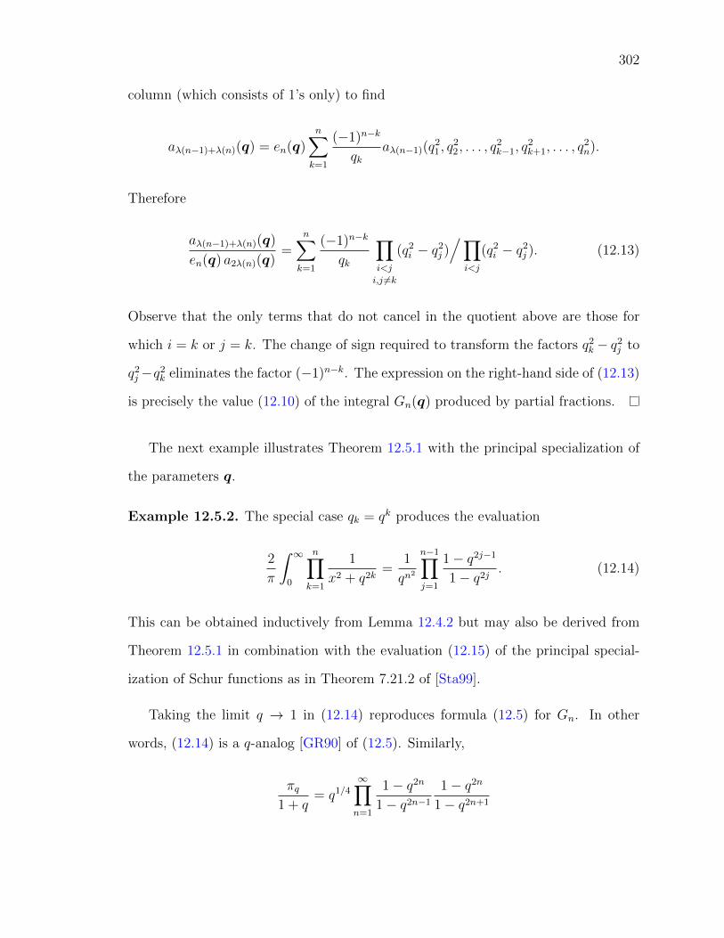
302
column (which consists of 1’s only) to find
aλ(n−1)+λ(n)(q) = en(q)n∑k=1
(−1)n−k
qkaλ(n−1)(q
21, q
22, . . . , q
2k−1, q
2k+1, . . . , q
2n).
Therefore
aλ(n−1)+λ(n)(q)
en(q) a2λ(n)(q)=
n∑k=1
(−1)n−k
qk
∏i<j
i,j 6=k
(q2i − q2
j )/∏
i<j
(q2i − q2
j ). (12.13)
Observe that the only terms that do not cancel in the quotient above are those for
which i = k or j = k. The change of sign required to transform the factors q2k − q2
j to
q2j−q2
k eliminates the factor (−1)n−k. The expression on the right-hand side of (12.13)
is precisely the value (12.10) of the integral Gn(q) produced by partial fractions.
The next example illustrates Theorem 12.5.1 with the principal specialization of
the parameters q.
Example 12.5.2. The special case qk = qk produces the evaluation
2
π
∫ ∞0
n∏k=1
1
x2 + q2k=
1
qn2
n−1∏j=1
1− q2j−1
1− q2j. (12.14)
This can be obtained inductively from Lemma 12.4.2 but may also be derived from
Theorem 12.5.1 in combination with the evaluation (12.15) of the principal special-
ization of Schur functions as in Theorem 7.21.2 of [Sta99].
Taking the limit q → 1 in (12.14) reproduces formula (12.5) for Gn. In other
words, (12.14) is a q-analog [GR90] of (12.5). Similarly,
πq1 + q
= q1/4
∞∏n=1
1− q2n
1− q2n−1
1− q2n
1− q2n+1
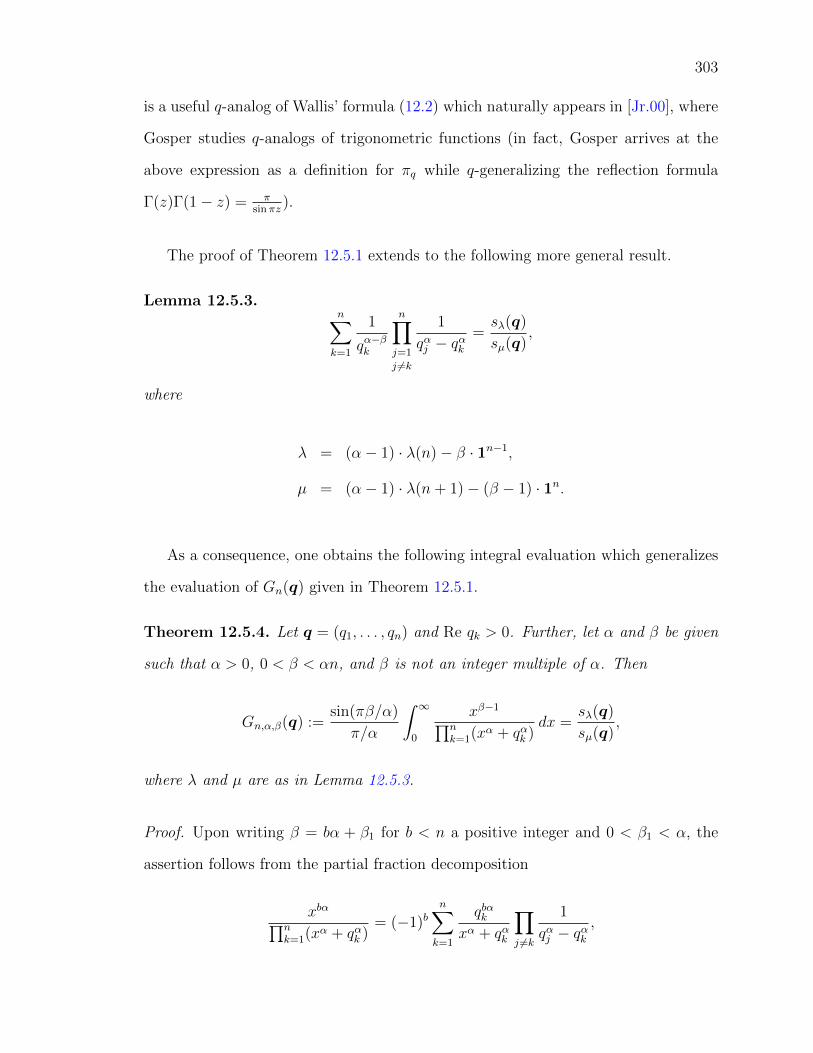
303
is a useful q-analog of Wallis’ formula (12.2) which naturally appears in [Jr.00], where
Gosper studies q-analogs of trigonometric functions (in fact, Gosper arrives at the
above expression as a definition for πq while q-generalizing the reflection formula
Γ(z)Γ(1− z) = πsinπz
).
The proof of Theorem 12.5.1 extends to the following more general result.
Lemma 12.5.3.n∑k=1
1
qα−βk
n∏j=1
j 6=k
1
qαj − qαk=sλ(q)
sµ(q),
where
λ = (α− 1) · λ(n)− β · 1n−1,
µ = (α− 1) · λ(n+ 1)− (β − 1) · 1n.
As a consequence, one obtains the following integral evaluation which generalizes
the evaluation of Gn(q) given in Theorem 12.5.1.
Theorem 12.5.4. Let q = (q1, . . . , qn) and Re qk > 0. Further, let α and β be given
such that α > 0, 0 < β < αn, and β is not an integer multiple of α. Then
Gn,α,β(q) :=sin(πβ/α)
π/α
∫ ∞0
xβ−1∏nk=1(xα + qαk )
dx =sλ(q)
sµ(q),
where λ and µ are as in Lemma 12.5.3.
Proof. Upon writing β = bα + β1 for b < n a positive integer and 0 < β1 < α, the
assertion follows from the partial fraction decomposition
xbα∏nk=1(xα + qαk )
= (−1)bn∑k=1
qbαkxα + qαk
∏j 6=k
1
qαj − qαk,

304
the integral evaluation
∫ ∞0
xβ1−1dx
xα + qα=
1
qα−β1π/α
sin(πβ1/α),
and Lemma 12.5.3.
12.6 Schur functions in terms of SSYT
The Schur function sλ(q) associated to a partition λ also admits a representation
in terms of semi-standard Young tableaux (SSYT). The reader will find information
about this topic in [Bre99]. Given a partition λ = (λ1, λ2, . . . , λm), the Young diagram
of shape λ is an array of boxes, arranged in left-justified rows, consisting of λ1 boxes
in the first row, λ2 in the second row, and so on, ending with λm boxes in the mth
row. A SSYT of shape λ is a Young diagram of shape λ in which the boxes have been
filled with positive integers. These integers are restricted to be weakly increasing
across rows (repetitions are allowed) and strictly increasing down columns. From this
point of view, the Schur function sλ(q) = sλ(q1, . . . , qn) can be defined as
sλ(q) =∑T
qT ,
where the sum is over all SSYT of shape λ with entries from {1, 2, . . . , n}. The symbol
qT is a monomial in the variables qj in which the exponent of qj is the number of
appearances of j in T . For example, the array shown in Figure 12.1 is a tableau T for
the partition (6, 4, 3, 3). The corresponding monomial qT is given by q1q32q3q
34q
45q
26q7q8.
The number Nn(λ) of SSYT of shape λ with entries from {1, 2, . . . , n} can be

305
1 2 2 4 5 52 3 4 54 6 65 7 8
Figure 12.1: A tableau T for the partition (6, 4, 3, 3).
obtained by letting q → 1 in the formula
sλ(1, q, q2, . . . , qn−1) =
∏1≤i<j≤n
qλi+n−i − qλj+n−jqj−1 − qi−1
(12.15)
(see page 375 of [Sta99]). This yields
Nn(λ) =∏
1≤i<j≤n
λi − λj + j − ij − i . (12.16)
The evaluation (12.5) of Wallis’ integral (12.3) may be recovered from here as
Gn+1 =sλ(n)(1
n+1)
sλ(n+2)(1n+1)
=Nn+1(λ(n))
Nn+1(λ(n+ 2))=
1
22n
(2n
n
).
12.7 A counting problem
The k-central binomial coefficients c(n, k), defined by the generating function
(1− k2x)−1/k =∑n≥0
c(n, k)xn,
are given by
c(n, k) =kn
n!
n−1∏m=1
(1 + km).
For k = 2 these coefficients reduce to the central binomial coefficients(
2nn
). The
numbers c(n, k) are integers in general and their divisibility properties have been

306
studied in [SMA09]. In particular, the authors establish that the k-central binomial
coefficients are always divisible by k and characterize their p-adic valuations.
The next result attempts an (admittedly somewhat contrived) interpretation of
what the numbers −c(n,−k) count.
Corollary 12.7.1. Let λ and µ be the partitions given by
λ = (k − 1) · λ(n)− 1n−1,
µ = (k − 1) · λ(n+ 1).
Then the integer −c(n,−k) enumerates the ratio between the total number of SSYT
of shapes λ and µ with entries from {1, 2, . . . , n} times the factor k2n−1/n.
Proof. By Theorem 12.5.4,
Nn(λ)
Nn(µ)=sλ(1
n)
sµ(1n)= Gn,k,1(1n) =
sin(π/k)
π/k
∫ ∞0
1
(xk + 1)ndx,
and the expression on the right-hand side is routine to evaluate:
Nn(λ)
Nn(µ)=
Γ(n− 1k)
Γ(n)Γ(1− 1k)
=n−1∏m=1
km− 1
km.
This product equals −c(n,−k) divided by k2n−1/n.
Remark 12.7.2. R. Stanley pointed out some interesting Schur function quotient
results. See exercises 7.30 and 7.32 in [Sta99].
12.8 An integral from Gradshteyn and Ryzhik
It is now demonstrated how the previous results may be used to prove an integral
evaluation found as entry 3.112 in [GR80]. The main tool is the (dual) Jacobi-Trudi

307
identity which expresses a Schur function in terms of elementary symmetric functions.
Namely, if λ is a partition such that its conjugate λ′ (the unique partition whose Young
diagram, see Section 12.6, is obtained from the one of λ by interchanging rows and
columns) has length at most m then
sλ =∣∣eλ′i−i+j∣∣16i,j6m .
This identity may be found for instance in [Sta99, Corollary 7.16.2].
Theorem 12.8.1. Let fn and gn be polynomials of the form
gn(x) = b0x2n−2 + b1x
2n−4 + . . .+ bn−1,
fn(x) = a0xn + a1x
n−1 + . . .+ an,
and assume that all roots of fn lie in the upper half-plane. Then
∫ ∞−∞
gn(x)dx
fn(x)fn(−x)=πi
a0
Mn
∆n
,
where
∆n =
∣∣∣∣∣∣∣∣∣∣∣∣∣∣∣∣
a1 a3 a5 . . . 0
a0 a2 a4 0
0 a1 a3 0
.... . .
0 0 0 an
∣∣∣∣∣∣∣∣∣∣∣∣∣∣∣∣, Mn =
∣∣∣∣∣∣∣∣∣∣∣∣∣∣∣∣
b0 b1 b2 . . . bn−1
a0 a2 a4 0
0 a1 a3 0
.... . .
0 0 0 an
∣∣∣∣∣∣∣∣∣∣∣∣∣∣∣∣.
Proof. Write fn(x) = a0
∏nj=1(x− iqj). By assumption, Re qj > 0. Further,
fn(x)fn(−x) = (−1)na20
n∏j=1
(x2 + q2j ).

308
Let q = (q1, q2, . . . , qn). It follows from Theorem 12.5.4 that
∫ ∞−∞
x2βdx
fn(x)fn(−x)=
(−1)n+βπ
a20
sλ(n−1)−2β·1n−1(q)
sλ(n+1)−2β·1n(q)=
(−1)nπ
a20
sλ′(q)
sλ(n+1)(q)
where λ = λ(n−1) + 2 ·1β. The latter equality is obtained by writing the quotient of
Schur functions as a quotient of alternants, multiplying the kth row of each matrix by
q2βk , and reordering the columns of the determinant in the numerator. The right-hand
side now is a quotient of Schur functions to which the Jacobi-Trudi identity may be
applied. In the denominator, this gives
sλ(n+1)(q) = |en+1−2k+j(q)|16k,j6n = |e2k−j(q)|16k,j6n .
Note that em(q) = 0 whenever m < 0 or m > n. Further, ek(q) = ikak/a0. Hence,
sλ(n+1)(q) = in(n+1)/2∆n/an0 . The term sλ′(q) is dealt with analogously. The claim
follows by expanding the determinant Mn with respect to the first row.
12.9 A sum related to Feynman diagrams
Particle scattering in quantum field theory is usually described in terms of Feyn-
man diagrams. A Feynman diagram is a graphical representation of a particular term
arising in the expansion of the relevant quantum-mechanical scattering amplitude
as a power series in the coupling constants that parametrize the strengths of the
interactions.
From the mathematical point of view, a Feynman diagram is a graph to which
a certain function is associated. If the graph has circuits (loops, in the physics ter-
minology) then this function is defined in terms of a number of integrals over the

309
4-dimensional momentum space (k0,k), where k0 is the energy integration variable
and k is a 3-dimensional momentum variable.
Feynman diagrams also appear in calculations of the thermodynamic properties
of a system described by quantum fields. In this context, the integral over the energy
component of a Feynman loop diagram is replaced by a summation over discrete
energy values. These Matsubara sums were introduced in [Mat55]. A general method
to compute these sums in terms of an associated integral was presented in [Esp10].
These techniques, applied to the expression (12.10) for the integral Gn(q), give
the value of the sum associated with the one-loop Feynman diagram consisting of n
vertices and vanishing external momenta, Ni = 0, as depicted in Figure 12.2.
Figure 12.2: The one-loop Feynman diagram with n vertices and vanishing externalmomenta. m is the summation variable associated to each of the internal lines.
The Matsubara sum associated to the diagram in Figure 12.2 is
Mn(q) :=∞∑
m=−∞
n∏k=1
1
m2 + q2k
, (12.17)
where the variables qk are related to the kinematic energies carried by the (virtual)
particles in the Feynman diagram. This sum was denoted by SG in [Esp10]; the
notation has been changed here to avoid confusion.

310
Example 12.9.1. The first few Matsubara sums are
M1(q1) = πD1
q1
,
M2(q1, q2) = πq2D1 − q1D2
q1q2(q22 − q2
1),
M3(q1, q2, q3) = πq2q3(q2
2 − q23)D1 + q3q1(q2
3 − q21)D2 + q1q2(q2
1 − q22)D3
q1q2q3(q23 − q2
2)(q22 − q2
1)(q21 − q2
3),
with Dj = coth(πqj).
Theorem 12.9.2. The Matsubara sum Mn(q) is given by
Mn(q) = πn∑k=1
coth(πqk)
qk
n∏j=1
j 6=k
1
q2j − q2
k
.
Proof 1. This follows from the partial fraction expansion
n∏k=1
1
m2 + q2k
=n∑k=1
1
q2k +m2
∏j 6=k
1
q2j − q2
k
,
which is a special case of (12.11), switching the order of summation, and employing
the classical
π coth(πz)
z=
∞∑m=−∞
1
z2 +m2.
Proof 2. The method developed in [Esp10] shows that
Mn(q) = π
[1 +
n∑m=1
nb(qm)(1−Rm)
]Gn(q), (12.18)
where Gn(q) is the integral defined in (12.9),
nb(q) =1
e2πq − 1=
1
2(cothπq − 1) ,

311
and Rm is the reflection operator defined by
Rmf(q1, . . . , qm, . . .) = f(q1, . . . ,−qm, . . .).
To use (12.18) combined with the evaluation (12.10) of Gn(q) it is required to compute
the action of each 1−Rm on the summands of (12.10). Namely,
(1−Rm)1
qk
n∏j=1
j 6=k
1
q2j − q2
k
=2δkmqk
n∏j=1
j 6=k
1
q2j − q2
k
,
where δkm is the Kronecker delta. Therefore
nb(qm)(1−Rm)Gn(q) =2 nb(qm)
qm
n∏j=1
j 6=m
1
q2j − q2
m
,
and the result follows from 2 nb(q) = coth(πq)− 1.
Finally, an expansion of Mn(q) in terms of symmetric functions is given. Starting
with the classical expansion
π coth qkqk
=1
q2k
− 2∞∑m=1
(−1)mq2m−2k ζ(2m),
where ζ(s) denotes the Riemann zeta function, it follows that
Mn(q) =n∑k=1
1
q2k
∏j 6=k
1
q2j − q2
k
− 2∞∑m=1
(−1)mζ(2m)n∑k=1
q2(m−1)k
∏j 6=k
1
q2j − q2
k
.
Using the identity (hj being the complete homogeneous symmetric function)
hm−n(x1, . . . , xn) = (−1)n−1
n∑k=1
xm−1k
∏j 6=k
1
xj − xk,

312
which follows from Lemma 12.5.3 (or see page 450, Exercise 7.4 of [Sta99]), this
proves:
Corollary 12.9.3. The Matsubara sum Mn(q), defined in (12.17), is given by
Mn(q) =1
en(q2)+ 2
∞∑m=0
(−1)mζ(2m+ 2n)hm(q2).
12.10 Conclusions
The evaluation of definite integrals has the charming quality of taking the reader
for a tour of many parts of mathematics. An innocent-looking generalization of one
of the oldest formulas in analysis has been shown to connect the work of the four
authors in the title.

313
Chapter 13
A sinc that sank
The contents of this chapter (apart from minor corrections or adaptions) have
been published as:
[BBS12] A sinc that sank(with David Borwein, Jonathan M. Borwein)
to appear in American Mathematical Monthly, Vol. 119, Nr. 7, Aug-Sep 2012
Abstract We resolve and further study a sinc integral evaluation, first posed in this
Monthly in [1967, p. 1015], which was solved in [1968, p. 914] and withdrawn in
[1970, p. 657]. After a short introduction to the problem and its history, we give a
general evaluation which we make entirely explicit in the case of the product of three
sinc functions. Finally, we exhibit some more general structure of the integrals in
question.
13.1 Introduction and background
In [1967, #5529, p. 1015] D. Mitrinovic asked in this Monthly for an evaluation
of
In :=
∫ ∞−∞
n∏j=1
sin (kj(x− aj))x− aj
dx (13.1)

314
for real numbers aj, kj with 1 6 j 6 n. We shall write In
(a1,...,ank1,...,kn
)when we wish to
emphasize the dependence on the parameters. Up to a constant factor, (13.1) is an
integral over a product of sinc functions: sinc x := sinxx
.
The next year a solution [1968, #5529, p. 914] was published in the form of
In = πn∏j=2
sin (kj(a1 − aj))a1 − aj
(13.2)
under the assumption that k1 > k2 > . . . > kn > 0. This solution, as M. Klamkin
pointed out in [1970, p. 657], can not be correct, since it is not symmetric in the
parameters while In is. Indeed, in the case k1 = k2 = k3 = 1 the evaluation (13.2)
is not symmetric in the variables aj and gives differing answers on permuting the
a’s. The proof given relies on formally correct Fourier analysis; but there are missing
constraints on the kj variables which have the effect that it is seldom right for more
than two variables. Indeed, as shown then by D. Djokovic and L. Glasser [Gla11]
— who were both working in Waterloo at the time — the evaluation (13.2) holds
true under the restriction k1 > k2 + k3 + . . . + kn when all of the kj are positive.
However, no simple general fix appeared possible — and indeed for n > 2 the issue is
somewhat complex. The problem while recorded several times in later Monthly lists
of unsolved problems appears (from a JSTOR hunt1) to have disappeared without
trace in the later 1980’s.
The precise issues regarding evaluation of sinc integrals are described in detail in
[BB01] or [BBG04, Chapter 2] along with some remarkable consequences [BBB08,
BB01, BBG04]. In the two-variable case, the 1968 solution is essentially correct; we
do obtain
I2 = πsin ((k1 ∧ k2)(a1 − a2))
a1 − a2
(13.3)
1A search on JSTOR through all Monthly volumes, suggests that the solutions were neverpublished and indeed for some years the original problem reappeared on lists of unsolved Monthlyproblems before apparently disappearing from view. Such a JSTOR search is not totally convincingsince there is no complete indexing of problems and their status.

315
for a1 6= a2 as will be made explicit below. Here a ∧ b := min{a, b}. Some of the
delicacy is a consequence of the fact that the classical sinc evaluation given next is
only conditionally true [BB01]. We have
∫ ∞−∞
sin(kx)
xdx = π sgn(k), (13.4)
where sgn(0) = 0, sgn(k) = 1 for k > 0 and sgn(k) = −1 for k < 0.
In (13.4) the integral is absolutely divergent and is best interpreted as a Cauchy-
Riemann limit. Thus the evaluation of (13.1) yields I1 = π sgn(k1) which has a
discontinuity at k1 = 0. For n > 2, however, In is an absolutely convergent integral
which is (jointly) continuous as a function of all kj and all aj. This follows from
Lebesgue’s dominated convergence theorem since the absolute value of the integrand
is less than∏n
j=1 |kj| for all x and less than 2/x2 for all sufficiently large |x|.
It is worth observing that the oscillatory structure of the integrals, see Figure 13.1,
means that their evaluation both numerically and symbolically calls for a significant
amount of care.
-Π Π
-0.05
0.05
0.1
Figure 13.1: Integrand in (13.1) with a = (−3,−2,−1, 0, 1, 2), k = (1, 2, 3, 4, 5, 6)
We wish to emphasize the continuing fascination with similar sinc integrals [GNJ87].
Indeed, the work in [BB01] was triggered by the exact problem described by K. Morri-

316
son in this Monthly [Mor95]. This led also to a lovely Monthly article on random
series [Sch03], and there is further related work in [BG02].
A most satisfactory introduction to the many applications and properties of the
sinc function is given in [GS90]. Additionally, T. Feeman’s recent book on medical
imaging [Fee10] chose to begin with the example given at the beginning of Section 13.4.
The paper [MM08b] makes a careful and historically informed study of the geometric
results implicit in the study of related multiple sinc integrals. This includes recording
that G. Polya in his 1912 doctoral thesis showed that if k = (k1, . . . , kn) has nonzero
coefficients and
Sk(θ) := {x ∈ Rn : |〈k, x〉| 6 θ/2, x ∈ Cn}
denotes the slab inside the hypercube Cn =[−1
2, 1
2
]ncut off by the hyperplanes
〈k, x〉 = ±θ/2, then
Voln(Sk(θ)) =1
π
∫ ∞−∞
sin(θx)
x
n∏j=1
sin(kjx)
kjxdx, (13.5)
a relationship we return to in Section 13.4. More general polyhedra volumes deter-
mined by multidimensional sinc integrals are examined in [BBM02]. As a consequence
of (13.5) and described for instance in [BB01], the integral (13.5) may also be inter-
preted as the probability that ∣∣∣∣∣n∑j=1
kjXj
∣∣∣∣∣ 6 θ (13.6)
where Xj are independent random variables uniformly distributed on [−1, 1].
13.2 Evaluation of In
Without loss of generality, we assume that all kj are strictly positive. In this
section, we shall only consider the case when all the aj are distinct. As illustrated

317
in Sections 13.3.2 and 13.3.3, the special cases can be treated by taking limits. We
begin with the classical and simple partial fraction expression
n∏j=1
1
x− aj=
n∑j=1
1
x− aj∏i 6=j
1
aj − ai(13.7)
valid when the aj are distinct. Applying (13.7) to the integral In we then have
In =n∑j=1
∫ ∞−∞
sin(kj(x− aj))x− aj
∏i 6=j
sin(ki(x− ai))aj − ai
dx
=n∑j=1
∫ ∞−∞
sin(kjx)
x
∏i 6=j
sin(ki(x+ (aj − ai)))aj − ai
dx. (13.8)
We pause and illustrate the general approach in the case of n = 2 variables.
Example 13.2.1 (Two variables). We apply (13.8) to write
I2 =
∫ ∞−∞
sin(k1x)
x
sin (k2(x+ a1 − a2))
a2 − a1
dx
+
∫ ∞−∞
sin(k2x)
x
sin (k1(x+ a2 − a1))
a1 − a2
dx
=sin (k2(a1 − a2))
a1 − a2
∫ ∞−∞
sin(k1x)
xcos(k2x) dx
+sin (k1(a2 − a1))
a2 − a1
∫ ∞−∞
sin(k2x)
xcos(k1x) dx
where for the second equation we have used the addition formula for the sine and
noticed that the sine-only integrands (being odd) integrate to zero. Finally, we either
appeal to [BB01, Theorem 3] or express
∫ ∞−∞
sin(k1x)
xcos(k2x) dx =
1
2
∫ ∞−∞
sin ((k1 + k2)x)
xdx
+1
2
∫ ∞−∞
sin ((k1 − k2)x)
xdx,

318
and appeal twice to (13.4) to obtain the final elegant cancellation
I2 = πsin ((k1 ∧ k2)(a1 − a2))
a1 − a2
(13.9)
valid for a1 6= a2. We observe that the result remains true for a1 = a2, in which case
the right-hand side of (13.9) attains the limiting value π(k1 ∧ k2). ♦
Let us observe that after the first step in Example 13.2.1 — independent of the
exact final formula — the integrals to be obtained have lost their dependence on the
aj. This is what we exploit more generally. Proceeding as in Example 13.2.1 and
applying the addition formula to (13.8) we write,
In =n∑j=1
∑A,B
Cj,A,B αj,A,B (13.10)
where the sum is over all sets A and B partitioning {1, 2 . . . , j − 1, j + 1, . . . n}, and
Cj,A,B :=∏i∈A
cos(ki(aj − ai))aj − ai
∏i∈B
sin(ki(aj − ai))aj − ai
(13.11)
while
αj,A,B :=
∫ ∞−∞
∏i∈A∪{j}
sin(kix)∏i∈B
cos(kix)dx
x. (13.12)
Notice that we may assume the cardinality |A| of A to be even since the integral in
(13.12) vanishes if |A| is odd.
To further treat (13.10), we write the products of sines and cosines in terms of
sums of single trigonometric functions. The general formulae are made explicit next.

319
Proposition 13.2.2 (Cosine product).
r∏j=1
cos(xj) = 2−r∑
ε∈{−1,1}rcos
(r∑j=1
εjxj
). (13.13)
Proof. The formula follows from the trigonometric identity 2 cos(a) cos(b) = cos(a +
b) + cos(a− b) applied inductively.
Observe that by taking derivatives with respect to some of the xj in (13.13), we
obtain similar formulae for general products of sines and cosines.
Corollary 13.2.3 (Sine and cosine product).
s∏j=1
sin(xj)r∏
j=s+1
cos(xj) = 2−r∑
ε∈{−1,1}r
(s∏j=1
εi
)cos
(r∑j=1
εjxj −sπ
2
). (13.14)
Here, we used ddx
cos(x) = cos(x− π/2) to write the evaluation rather compactly.
Note that when s = 2k+1 is odd then cos(x−sπ/2) = (−1)k sin(x). Applying (13.14)
to the definition (13.12), it thus follows that, for even |A|,
αj,A,B = (−1)|A|/2∫ ∞−∞
1
2n
∑ε∈{−1,1}n
∏i∈A∪{j}
εi
sin
(n∑i=1
εikix
)dx
x
= π (−1)|A|/21
2n
∑ε∈{−1,1}n
∏i∈A∪{j}
εi
sgn
(n∑i=1
εiki
). (13.15)
Then, on combining (13.15) with (13.10), we obtain the following general evaluation.
Theorem 13.2.4 (General evaluation). We have
In =n∑j=1
∑A,B
αj,A,B Cj,A,B (13.16)
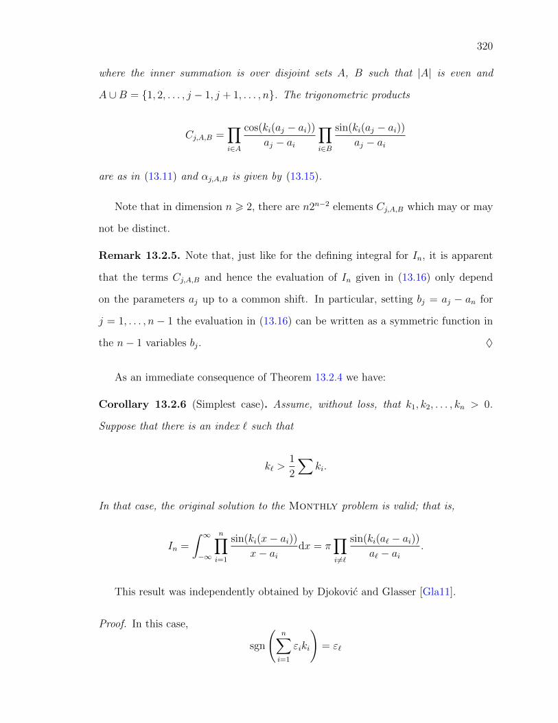
320
where the inner summation is over disjoint sets A, B such that |A| is even and
A ∪B = {1, 2, . . . , j − 1, j + 1, . . . , n}. The trigonometric products
Cj,A,B =∏i∈A
cos(ki(aj − ai))aj − ai
∏i∈B
sin(ki(aj − ai))aj − ai
are as in (13.11) and αj,A,B is given by (13.15).
Note that in dimension n > 2, there are n2n−2 elements Cj,A,B which may or may
not be distinct.
Remark 13.2.5. Note that, just like for the defining integral for In, it is apparent
that the terms Cj,A,B and hence the evaluation of In given in (13.16) only depend
on the parameters aj up to a common shift. In particular, setting bj = aj − an for
j = 1, . . . , n− 1 the evaluation in (13.16) can be written as a symmetric function in
the n− 1 variables bj. ♦
As an immediate consequence of Theorem 13.2.4 we have:
Corollary 13.2.6 (Simplest case). Assume, without loss, that k1, k2, . . . , kn > 0.
Suppose that there is an index ` such that
k` >1
2
∑ki.
In that case, the original solution to the Monthly problem is valid; that is,
In =
∫ ∞−∞
n∏i=1
sin(ki(x− ai))x− ai
dx = π∏i 6=`
sin(ki(a` − ai))a` − ai
.
This result was independently obtained by Djokovic and Glasser [Gla11].
Proof. In this case,
sgn
(n∑i=1
εiki
)= ε`

321
for all values of the εi. The claim now follows from Theorem 13.2.4. More precisely,
if there is some index k 6= ` such that k ∈ A or j = k, then αj,A,B = 0. This is
because the term in (13.15) contributed by ε ∈ {−1, 1}n has opposite sign than the
term contributed by ε′, where ε′ is obtained from ε by flipping the sign of εk. It
remains to observe that α`,∅,B = π according to (13.15). This is the only surviving
term.
13.2.1 Alternative evaluation of In
In 1970 Djokovic sent in a solution to the Monthly after the original solution
was withdrawn [Gla11]. He used the following identity involving the principal value
(PV) of the integral
(PV)
∫ ∞−∞
eitx
x− ajdx = lim
δ→0+
{∫ aj−δ
−∞+
∫ ∞aj+δ
}eitx
x− ajdx = πi sgn(t)eitaj
where t is real. Note that setting aj = 0 and taking the imaginary part gives (13.4).
He then showed, using the same partial fraction expansion as above, that
In =πi
(2i)n
n∑j=1
{Aj
∑ε∈{−1,1}n
(n∏r=1
εr
)sgn
(n∑r=1
εrkr
)(13.17)
· exp
(i
n∑r=1
εrkr(aj − ar))}
where a1, a2, . . . , an are distinct and
Aj :=1∏
r 6=j(aj − ar). (13.18)
The formula (13.17) is quite elegant and also allows one to derive Corollary 13.2.6,
which was independently found by Glasser [Gla11]. For instance, it suffices to appeal
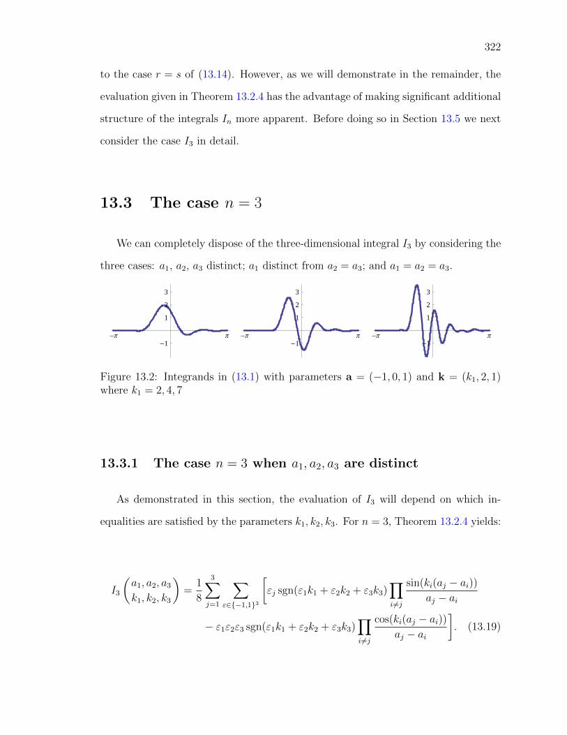
322
to the case r = s of (13.14). However, as we will demonstrate in the remainder, the
evaluation given in Theorem 13.2.4 has the advantage of making significant additional
structure of the integrals In more apparent. Before doing so in Section 13.5 we next
consider the case I3 in detail.
13.3 The case n = 3
We can completely dispose of the three-dimensional integral I3 by considering the
three cases: a1, a2, a3 distinct; a1 distinct from a2 = a3; and a1 = a2 = a3.
-Π Π-1
1
2
3
-Π Π-1
1
2
3
-Π Π-1
1
2
3
Figure 13.2: Integrands in (13.1) with parameters a = (−1, 0, 1) and k = (k1, 2, 1)where k1 = 2, 4, 7
13.3.1 The case n = 3 when a1, a2, a3 are distinct
As demonstrated in this section, the evaluation of I3 will depend on which in-
equalities are satisfied by the parameters k1, k2, k3. For n = 3, Theorem 13.2.4 yields:
I3
(a1, a2, a3
k1, k2, k3
)=
1
8
3∑j=1
∑ε∈{−1,1}3
[εj sgn(ε1k1 + ε2k2 + ε3k3)
∏i 6=j
sin(ki(aj − ai))aj − ai
− ε1ε2ε3 sgn(ε1k1 + ε2k2 + ε3k3)∏i 6=j
cos(ki(aj − ai))aj − ai
]. (13.19)

323
Remark 13.3.1 (Recovering Djokovic’s evaluation). Upon using the trigonometric
identity sin(x) sin(y)− cos(x) cos(y) = − cos(x+ y) to combine the two products, the
right-hand side of equation (13.19) can be reexpressed in the symmetric form
−1
8
∑ε∈{−1,1}3
ε1ε2ε3 sgn(ε1k1 + ε2k2 + ε3k3)3∑j=1
cos(∑
i 6=j εiki(aj − ai))∏i 6=j(aj − ai)
.
This is precisely Djokovic’s evaluation (13.17). ♦
In fact, distinguishing between two cases, illustrated in Figure 13.3, the evaluation
(13.19) of I3 can be made entirely explicit:
Corollary 13.3.2 (a1, a2, a3 distinct). Assume that k1, k2, k3 > 0. Then
1. If 12
∑ki 6 k`, as can happen for at most one index `, then
I3
(a1, a2, a3
k1, k2, k3
)= π
∏i 6=`
sin(ki(a` − ai))a` − ai
. (13.20)
2. Otherwise, that is if max ki <12
∑ki, then
I3
(a1, a2, a3
k1, k2, k3
)=π
2
3∑j=1
[∏i 6=j
sin(ki(aj − ai))aj − ai
+∏i 6=j
cos(ki(aj − ai))aj − ai
]. (13.21)
Proof. The first case is a special case of Corollary 13.2.6. Alternatively, assuming
without loss that the inequality for k` is strict, it follows directly from (13.19) (because
sgn(ε1k1 + ε2k2 + ε3k3) = ε`, all but one sum over ε ∈ {−1, 1}3 cancel to zero).
In the second case, k1 < k2 + k3, k2 < k3 + k1, k3 < k1 + k2. Therefore
1
8
∑ε∈{−1,1}3
εj sgn(ε1k1 + ε2k2 + ε3k3) =1
2for all j,
−1
8
∑ε∈{−1,1}3
ε1ε2ε3 sgn(ε1k1 + ε2k2 + ε3k3) =1
2.

324
ℓ = 3 ℓ = 1
ℓ = 2
k3
k2k2
0 k3 k1k1
Figure 13.3: The constraints on the parameters kj in Corollary 13.3.2 — if k1, k2 takevalues in the shaded regions then (13.20) holds with the indicated choice of `
The claim then follows from (13.19).
Remark 13.3.3 (Hidden trigonometric identities). Observe that because of the con-
tinuity of I3 as a function of k1, k2, and k3, we must have the nonobvious identity
∏i 6=1
[sin(ki(a1 − ai))
a1 − ai
]=
1
2
3∑j=1
[∏i 6=j
sin(ki(aj − ai))aj − ai
+∏i 6=j
cos(ki(aj − ai))aj − ai
](13.22)
when k1 = k2 + k3. We record that Mathematica 7 is able to verify (13.22); however,
it struggles with the analogous identities arising for n > 4. ♦
13.3.2 The case n = 3 when a1 6= a2 = a3
As a limiting case of Corollary 13.3.2 we obtain the following.
Corollary 13.3.4 (a1 6= a2 = a3). Assume that k1, k2, k3 > 0 and a1 6= a2. Set
a := a2 − a1.

325
1. If k1 > 12
∑ki, then
I3
(a1, a2, a2
k1, k2, k3
)= π
sin(k2a)
a
sin(k3a)
a. (13.23)
2. If max(k2, k3) > 12
∑ki, then
I3
(a1, a2, a2
k1, k2, k3
)= πmin(k2, k3)
sin(k1a)
a. (13.24)
3. Otherwise, that is if max ki <12
∑ki, then
I3
(a1, a2, a2
k1, k2, k3
)=π
2
cos((k2 − k3)a)− cos(k1a)
a2+π
2
(k2 + k3 − k1) sin(k1a)
a.
(13.25)
Proof. The first two cases are immediate consequences of (13.20) upon taking the
limit a3 → a2.
Likewise, the third case follows from (13.21) with just a little bit of care. The
contribution of the sine products from (13.21) is
π
2
sin(k2a) sin(k3a)
a2+π
2
(k2 + k3) sin(k1a)
a.
On the other hand, writing a3 = a2 + ε with the intent of letting ε → 0, the cosine
products contribute
π
2
[cos(k2a) cos(k3a)
a2− cos(k1a) cos(k3ε)
aε+
cos(k1(a+ ε)) cos(k2ε)
(a+ ε)ε
].
The claim therefore follows once we show
cos(k1a) cos(k3ε)
aε− cos(k1(a+ ε)) cos(k2ε)
(a+ ε)ε→ cos(k1a)
a2+k1 sin(k1a)
a.

326
This is easily verified by expanding the left-hand side in a Taylor series with respect
to ε. In fact, all the steps in this proof can be done automatically using, for instance,
Mathematica 7.
Observe that, since In is invariant under changing the order of its arguments,
Corollary 13.3.4 covers all cases where exactly two of the parameters aj agree.
Remark 13.3.5 (Alternative approach). We remark that Corollary 13.3.4 can al-
ternatively be proved in analogy with the proof given for Theorem 13.2.4 — that is
by starting with a partial fraction decomposition and evaluating the occurring basic
integrals. Besides integrals covered by equation (13.15), this includes formulae such
as
∫ ∞−∞
sin(k2x)
x
sin(k3x)
xcos(k1x)dx
=π
8
∑ε∈{−1,1}3
ε2ε3(ε1k1 + ε2k2 + ε3k3) sgn(ε1k1 + ε2k2 + ε3k3). (13.26)
This evaluation follows from [BB01, Theorem 3(ii)]. In fact, (13.26) is an immediate
consequence of equation (13.15) with n = 3 and A = ∅ after integrating with respect
to one of the parameters ki where i ∈ B. Clearly, this strategy evaluates a large class
of integrals, similar to (13.26), over the real line with integrands products of sines
and cosines as well as powers of the integration variable (see also [BB01]). ♦
13.3.3 The case n = 3 when a1 = a2 = a3
In this case,
I3 =
∫ ∞−∞
sin(k1(x− a1))
x− a1
sin(k2(x− a1))
x− a1
sin(k3(x− a1))
x− a1
dx
=
∫ ∞−∞
sin(k1x)
x
sin(k2x)
x
sin(k3x)
xdx. (13.27)

327
Corollary 13.3.6 (a1 = a2 = a3). Assume, without loss, that k1 > k2 > k3 > 0.
Then
1. If k1 > k2 + k3, then
I3
(a1, a1, a1
k1, k2, k3
)= π k2k3.
2. If k1 6 k2 + k3, then
I3
(a1, a1, a1
k1, k2, k3
)= π
(k2k3 −
(k2 + k3 − k1)2
4
).
Proof. The first part follows from Theorem 2 and the second from Corollary 1 in
[BB01].
Alternatively, Corollary 13.3.6 may be derived from Corollary 13.3.4 on letting a
tend to zero. Again, this can be automatically done in a computer algebra system
such as Mathematica 7 or Maple 14.
13.4 Especially special cases of sinc integrals
The same phenomenon as in equation (13.5) and in Corollary 13.3.6 leads to
one of the most striking examples in [BB01]. Consider the following example of a
re-normalized In integral, in which we set
Jn :=
∫ ∞−∞
sincx · sinc(x
3
)· · · sinc
(x
2n+ 1
)dx.
328
Then — as Maple and Mathematica are able to confirm — we have the following
evaluations:
J0 =
∫ ∞−∞
sincx dx = π,
J1 =
∫ ∞−∞
sincx · sinc(x
3
)dx = π,
...
J6 =
∫ ∞−∞
sincx · sinc(x
3
)· · · sinc
( x13
)dx = π.
As explained in detail in [BB01] or [BBG04, Chapter 2], the seemingly obvious
pattern — a consequence of Corollary 13.2.6 — is then confounded by
J7 =
∫ ∞−∞
sincx · sinc(x
3
)· · · sinc
( x15
)dx
=467807924713440738696537864469
467807924720320453655260875000π < π,
where the fraction is approximately 0.99999999998529 . . . which, depending on the
precision of calculation, numerically might not even be distinguished from 1.
This is a consequence of the following general evaluation given in [BB01].
Theorem 13.4.1 (First bite). Denote Km = k0 + k1 + . . .+ km. If 2kj > kn > 0 for
j = 0, 1, . . . , n− 1 and Kn > 2k0 > Kn−1, then
∫ ∞−∞
n∏j=0
sin(kjx)
xdx = πk1k2 · · · kn −
π
2n−1n!(Kn − 2k0)n. (13.28)
Note that Theorem 13.4.1 is a “first-bite” extension of Corollary 13.2.6; assuming
only that kj > 0 for j = 0, 1, . . . , n then if 2k0 > Kn the integral evaluates to
πk1k2 · · · kn.

329
Theorem 13.4.1 makes clear that the pattern Jn = π for n = 0, 1, . . . , 6 breaks for
J7 because
1
3+
1
5+ . . .+
1
15> 1
whereas all earlier partial sums are less than 1. Geometrically, the situation is as
follows. In light of (13.5), the integral Jn may be interpreted as the volume of the
part of a hypercube lying between two planes. For n = 7 these planes intersect with
the hypercube for the first time.
Example 13.4.2 (A probabilistic interpretation). Let us illustrate Theorem 13.4.1
using the probabilistic point of view mentioned in (13.6) at the end of the introduction.
As such the integral
1
π
∫ ∞−∞
sin(k0x)
x
sin(k1x)
k1x
sin(k2x)
k2xdx
is the probability that |k1X1 + k2X2| 6 k0 where X1, X2 are independent random
variables distributed uniformly on [−1, 1].
-1-
2
30 2
31
-1
-
1
2
1
2
1
Figure 13.4: The event |3X1 + 2X2| 6 4
In the case k0 = 4, k1 = 3, k2 = 2, for example, this event is represented as the
shaded area in Figure 13.4. Since each of the removed triangular corners has sides

330
of length 1/2 and 1/3, this region has area 23/6. Because the total area is 4, the
probability of the event in question is 23/24. Thus,
1
π
∫ ∞−∞
sin(4x)
x
sin(3x)
3x
sin(2x)
2xdx =
23
24=
1
3 · 2
(3 · 2− (3 + 2− 4)2
2 · 2
)
in agreement with Theorem 13.4.1. ♦
Let us return to the example of the integrals Jn. Even past n = 7, we do have
a surprising equality [BBB08] of these integrals and corresponding Riemann sums.
This alternative evaluation of the integrals Jn is
∫ ∞−∞
n∏j=0
sinc
(x
2j + 1
)dx =
∞∑m=−∞
n∏j=0
sinc
(m
2j + 1
)(13.29)
which is valid for n = 1, 2, . . . , 7, 8, . . . , 40248. The “first-bite” phenomenon is seen
here again but at larger n. For n > 40248 this equality fails as well; the sum being
strictly bigger than the integral. As in the case of (13.28), there is nothing special
about the choice of parameters kj = 12j+1
in the sinc functions. Indeed, the following
general result is proved in [BBB08].
Theorem 13.4.3. Suppose that k1, k2, . . . , kn > 0. If k1 + k2 + . . .+ kn < 2π, then
∫ ∞−∞
n∏j=1
sinc(kjx) dx =∞∑
m=−∞
n∏j=1
sinc(kjm). (13.30)
Note that the condition k1 + k2 + . . . + kn < 2π may always be satisfied through
a common rescaling kj → τkj of the parameters kj at the expense of writing the sinc
integral as a sinc sum with differently scaled parameters.
As a consequence of Theorem 13.4.3, we see that (13.29) holds for n provided that
n∑j=0
1
2j + 1< 2π

331
which is true precisely for the range of n specified above.
Remark 13.4.4. With this insight, it is not hard to contrive more persistent exam-
ples. An entertaining example given in [BBB08] is taking the reciprocals of primes.
Using the Prime Number Theorem, one estimates that the sinc integrals equal the
sinc sums until the number of products is about 10176. That of course makes it rather
unlikely to find, by mere testing, an example where the two are unequal. Even worse
for the naive tester is the fact that the discrepancy between integral and sum is always
less than 10−1086 (and even smaller if the Riemann hypothesis is true). ♦
A related integral, which because of its varied applications has appeared repeat-
edly in the literature, see e.g. [MR65] and the references therein, is
2
π
∫ ∞0
(sinx
x
)ncos(bx) dx (13.31)
which, for 0 6 b < n, has the closed form
1
2n−1(n− 1)!
∑06k<(n+b)/2
(−1)k(n
k
)(n+ b− 2k)n−1.
To give an idea of the range of applications, we only note that the authors of [MR65]
considered the integral (13.31) because it is proportional to “the intermodulation
distortion generated by taking the nth power of a narrow-band, high-frequency white
noise”; on the other hand, the recent [Ali08] uses (13.31) with b = 0 to obtain an
improved lower bound for the Erdos-Moser problem.
If b > n, then the integral (13.31) vanishes. The case b = 0 in (13.31) is the
interesting special case of In with k1 = . . . = kn = 1 and a1, . . . , an = 0. Its evaluation
appears as an exercise in [WW27, p. 123]; in [BB01] it is demonstrated how it may
be derived using the present methods.

332
13.5 The case n > 4
Returning to Theorem 13.2.4, we now show — somewhat briefly — that in certain
general cases the evaluation of the integral In may in essence be reduced to the evalua-
tion of the integral Im for some m < n. In particular, we will see that Corollary 13.2.6
is the most basic such case — corresponding to m = 1.
In order to exhibit this general structure of the integrals In, we introduce the
notation
In,j :=∑A,B
αj,A,B Cj,A,B (13.32)
so that, by (13.16), In =∑n
j=1 In,j.
Theorem 13.5.1 (Substructure). Assume that k1 > k2 > . . . > kn > 0, and that
a1, a2, . . . , an are distinct. Suppose that there is some m such that for all ε ∈ {−1, 1}n
we have
sgn(ε1k1 + . . .+ εmkm + . . .+ εnkn) = sgn(ε1k1 + . . .+ εmkm). (13.33)
Then
In =m∑j=1
Im,j∏i>m
sin(ki(aj − ai))aj − ai
. (13.34)
Proof. Note that in light of (13.15) and (13.33) we have αj,A,B = 0 unless {m +
1, . . . , n} ⊂ B. To see this, assume that there is some index k > m such that k ∈ A
or k = j. Then the term in (13.15) contributed by ε ∈ {−1, 1}n has opposite sign
as the term contributed by ε′, where ε′ is obtained from ε by flipping the sign of εk.
The claim now follows from Theorem 13.2.4.

333
Remark 13.5.2. The condition (13.33) may equivalently be stated as
min |ε1k1 + . . .+ εmkm| > km+1 + . . .+ kn (13.35)
where the minimum is taken over ε ∈ {−1, 1}m. We idly remark that, for large m,
computing this minimum is a hard problem. In fact, in the special case of integral
kj, just deciding whether the minimum is zero (which is equivalent to the partition
problem of deciding whether the parameters kj can be partitioned into two sets with
the same sum) is well-known to be NP-complete [GJ79, Section 3.1.5]. ♦
Observe that the case m = 1 of Theorem 13.5.1, together with the basic evaluation
(13.4), immediately implies Corollary 13.2.6. This is because the condition (13.33)
holds for m = 1 precisely if k1 > k2 + . . .+ kn.
If (13.33) holds for m = 2, then it actually holds for m = 1 provided that the
assumed inequality k1 > k2 is strict. Therefore the next interesting case is m = 3.
The final evaluation makes this case explicit. It follows from Corollary 13.3.2.
Corollary 13.5.3 (A second n-dimensional case). Let n > 3. Assume that k1 > k2 >
. . . > kn > 0, and that a1, a2, . . . , an are distinct. If
k1 6 k2 + . . .+ kn and k2 + k3 − k1 > k4 + . . .+ kn,
then
In =π
2
3∑j=1
∏i>4
sin(ki(aj − ai))aj − ai
[ ∏i63,i 6=j
sin(ki(aj − ai))aj − ai
+∏
i63,i 6=j
cos(ki(aj − ai))aj − ai
].
The cases m > 4 quickly become much more involved. In particular, the condition
(13.33) becomes a set of inequalities. To close, we illustrate with the first case not
covered by Corollaries 13.2.6 and 13.5.3:

334
Example 13.5.4. As usual, assume that k1 > k2 > k3 > k4 > 0, and that a1, a2, a3, a4
are distinct. If k1 < k2 +k3 +k4 (hence Corollary 13.2.6 does not apply) and k1 +k4 >
k2 + k3 (hence Corollary 13.5.3 does not apply either), then
I4 =π
4
4∑j=1
∑A,B
Cj,A,B +π
2
∏i 6=1
sin(ki(a1 − ai))a1 − ai
(13.36)
− π
2
4∑j=2
sin(k1(aj − a1))
aj − a1
∏i 6=1,j
cos(ki(aj − ai))aj − ai
where the summation in the first sum is as in Theorem 13.2.4. Note that the terms
I4,j of (13.32) are implicit in (13.36) and may be used to make the case m = 4 of
Theorem 13.5.1 explicit as has been done in Corollary 13.5.3 for m = 3. ♦
13.6 Conclusions
We present these results for several reasons. First is the intrinsic beauty and utility
of the sinc function. It is important in so many areas of computing, approximation
theory, and numerical analysis. It is used in interpolation and approximation of
functions, approximate evaluation of transforms — e.g., Hilbert, Fourier, Laplace,
Hankel, and Mellin transforms as well as the fast Fourier transform — see [Ste93].
It is used in approximating solutions of differential and integral equations, in image
processing [Fee10], in other signal processing and in information theory. It is the
Fourier transform of the box filter and so central to the understanding of the Gibbs
phenomenon [Str81] and its descendants. Much of this is nicely described in [GS90].
Second is that the forensic nature of the mathematics was entertaining. It also
made us reflect on how computer packages and databases have changed mathematics
over the past forty to fifty years. As our hunt for the history of this Monthly
problem indicates, better tools for searching our literature are much needed. Finally

335
some of the evaluations merit being better known as they are excellent tests of both
computer algebra and numerical integration.

336
Chapter 14
The p-adic valuation of k-centralbinomial coefficients
The contents of this chapter (apart from minor corrections or adaptions) have
been published as:
[SMA09] The p-adic valuation of k-central binomial coefficients(with Tewodros Amdeberhan, Victor H. Moll)
published in Acta Arithmetica, Vol. 140, 2009, p. 31-42
Abstract The coefficients c(n, k) defined by
(1− k2x)−1/k =∑n≥0
c(n, k)xn
reduce to the central binomial coefficients(
2nn
)for k = 2. Motivated by a question of
H. Montgomery and H. Shapiro for the case k = 3, we prove that c(n, k) are integers
and study their divisibility properties.
14.1 Introduction
In a recent issue of the American Mathematical Monthly, Hugh Montgomery and
Harold S. Shapiro proposed the following problem (Problem 11380, August-September
2008):
337
For x ∈ R, let (x
n
)=
1
n!
n−1∏j=0
(x− j). (14.1)
For n ≥ 1, let an be the numerator and qn the denominator of the rational number(−1/3n
)expressed as a reduced fraction, with qn > 0.
1. Show that qn is a power of 3.
2. Show that an is odd if and only if n is a sum of distinct powers of 4.
Our approach to this problem employs Legendre’s remarkable expression [Leg30]:
νp(n!) =n− sp(n)
p− 1, (14.2)
that relates the p-adic valuation of factorials to the sum of digits of n in base p. For
m ∈ N and a prime p, the p-adic valuation of m, denoted by νp(m), is the highest
power of p that divides m. The expansion of m ∈ N in base p is written as
m = a0 + a1p+ · · ·+ adpd, (14.3)
with integers 0 ≤ aj ≤ p− 1 and ad 6= 0. The function sp in (14.2) is defined by
sp(m) := a0 + a1 + · · ·+ ad. (14.4)
Since, for n > 1, νp(n) = νp(n!)− νp((n− 1)!), it follows from (14.2) that
νp(n) =1 + sp(n− 1)− sp(n)
p− 1. (14.5)
The p-adic valuations of binomial coefficients can be expressed in terms of the
function sp:
νp
((n
k
))=sp(k) + sp(n− k)− sp(n)
p− 1. (14.6)

338
In particular, for the central binomial coefficients Cn :=(
2nn
)and p = 2, we have
ν2 (Cn) = 2s2(n)− s2(2n) = s2(n). (14.7)
Therefore, Cn is always even and 12Cn is odd precisely whenever n is a power of 2.
This is a well-known result.
The central binomial coefficients Cn have the generating function
(1− 4x)−1/2 =∑n≥0
Cnxn. (14.8)
The binomial theorem shows that the numbers in the Montgomery-Shapiro problem
bear a similar generating function
(1− 9x)−1/3 =∑n≥0
(−13
n
)(−9x)n. (14.9)
It is natural to consider the coeffients c(n, k) defined by
(1− k2x)−1/k =∑n≥0
c(n, k)xn, (14.10)
which include the central binomial coefficients as a special case. We call c(n, k) the
k-central binomial coefficients. The expression
c(n, k) = (−1)n(− 1
k
n
)k2n (14.11)
comes directly from the binomial theorem. Thus, the Montgomery-Shapiro question
from (14.1) deals with arithmetic properties of
(−13
n
)= (−1)n
c(n, 3)
32n. (14.12)

339
14.2 The integrality of c(n, k)
It is a simple matter to verify that the coefficients c(n, k) are rational numbers.
The expression produced in the next proposition is then employed to prove that
c(n, k) are actually integers. The next section will explore divisibility properties of
the integers c(n, k).
Proposition 14.2.1. The coefficient c(n, k) is given by
c(n, k) =kn
n!
n−1∏m=1
(1 + km). (14.13)
Proof. The binomial theorem yields
(1− k2x)−1/k =∑n≥0
(− 1k
n
)(−k2x)n
=∑n≥0
kn
n!
(n−1∏m=1
(1 + km)
)xn,
and (14.13) has been established.
An alternative proof of the previous result is obtained from the simple recurrence
c(n+ 1, k) =k(1 + kn)
n+ 1c(n, k), for n ≥ 0, (14.14)
and its initial condition c(0, k) = 1. To prove (14.14), simply differentiate (14.10) to
produce
k(1− k2x)−1/k−1 =∑n≥0
(n+ 1)c(n+ 1, k)xn (14.15)
and multiply both sides by 1− k2x to get the result.
340
Note 14.2.2. The coefficients c(n, k) can be written in terms of the Beta function as
c(n, k) =k2n
nB(n, 1/k). (14.16)
This expression follows directly by writing the product in (14.13) in terms of the
Pochhammer symbol (a)n = a(a+ 1) · · · (a+ n− 1) and the identity
(a)n =Γ(a+ n)
Γ(a). (14.17)
The proof employs only the most elementary properties of the Euler’s Gamma and
Beta functions. The reader can find details in [BM04]. The conclusion is that we
have an integral expression for c(n, k), given by
c(n, k)
∫ 1
0
(1− u1/n)1/k−1 du = k2n. (14.18)
It is unclear how to use it to further investigate c(n, k).
In the case k = 2, we have that c(n, 2) = Cn is a positive integer. This result
extends to all values of k.
Theorem 14.2.3. The coefficient c(n, k) is a positive integer.
Proof. First observe that if p is a prime dividing k, then the product in (14.10) is
relatively prime to p. Therefore we need to check that νp(n!) ≤ νp(kn). This is simple:
νp(n!) =n− sp(n)
p− 1≤ n ≤ νp(k
n). (14.19)
Now let p be a prime not dividing k. Clearly,
νp(c(n, k)) = νp
(∏m<n
(1 + km)
)− νp
(∏m<n
(1 +m)
). (14.20)

341
To prove that c(n, k) is an integer, we compare the p-adic valuations of 1 + km and
1+m. Observe that 1+m is divisible by pα if and only if m is of the form λpα−1. On
the other hand, 1+km is divisible by pα precisely when m is of the form λpα− ipα(k),
where ipα(k) denotes the inverse of k modulo pα in the range 1, 2, · · · , pα − 1. Thus,
νp(c(n, k)) =∑α≥1
⌊n+ipα (k)−1
pα
⌋−⌊npα
⌋. (14.21)
The claim now follows from ipα(k) ≥ 1.
Next, Theorem 14.2.3 will be slightly strengthened and an alternative proof be
provided.
Theorem 14.2.4. For n > 0, the coefficient c(n, k) is a positive integer divisible by
k.
Proof. Expanding the right hand side of the identity
(1− k2x)−1 =((1− k2x)−1/k
)k(14.22)
by the Cauchy product formula gives
∑i1+···+ik=m
c(i1, k)c(i2, k) · · · c(ik, k) = k2m, (14.23)
where the multisum runs through all the k-tuples of non-negative integers. Obviously
c(0, k) = 1 and it is easy to check that c(1, k) = k. We proceed by induction on n,
so we assume the assertion is valid for c(1, k), c(2, k), · · · , c(n − 1, k). We prove the
same is true for c(n, k). To this end, break up (14.23) as
kc(n, k) +∑
i1+···+ik=n0≤ij<n
c(i1, k)c(i2, k) · · · c(ik, k) = k2n. (14.24)

342
Hence by the induction assumption kc(n, k) is an integer.
To complete the proof, divide (14.24) through by k2 and rewrite as follows
c(n, k)
k= k2n−2 − 1
k2
∑i1+···+ik=n
0≤ij<n
c(i1, k)c(i2, k) · · · c(ik, k). (14.25)
The key point is that each summand in (14.25) contains at least two terms, each one
divisible by k.
Note 14.2.5. W. Lang [Lan00] has studied the numbers appearing in the generating
function
c2(l;x) :=1− (1− l2x)1/l
lx, (14.26)
that bears close relation to the case k = −l < 0 of equation (14.10). The special
case l = 2 yields the Catalan numbers. The author establishes the integrality of the
coefficients in the expansion of c2 and other related functions.
14.3 The valuation of c(n, k)
We consider now the p-adic valuation of c(n, k). The special case when p divides
k is easy, so we deal with it first.
Proposition 14.3.1. Let p be a prime that divides k. Then
νp(c(n, p)) = νp(k)n− n− sp(n)
p− 1. (14.27)
Proof. The p-adic valuation of c(n, p) is given by
νp(c(n, p)) = νp(k)n− νp(n!) = νp(k)n− n− sp(n)
p− 1. (14.28)
343
Finally note that sp(n) = O(log n).
Note 14.3.2. For p, k 6= 2, we have νp(c(n, p)) ∼(νp(k)− 1
p−1
)n, as n→∞.
We now turn attention to the case where p does not divide k. Under this as-
sumption, the congruence kx ≡ 1 mod pα has a solution. Elementary arguments of
p-adic analysis can be used to produce a p-adic integer that yields the inverse of k.
This construction proceeds as follows: first choose b0 in the range {1, 2, · · · , p − 1}
to satisfy kb0 ≡ 1 mod p. Next, choose c1, satisfying kc1 ≡ 1 mod p2 and write it as
c1 = b0 + kb1 with 0 ≤ b1 ≤ p− 1. Proceeding in this manner, we obtain a sequence
of integers {bj : j ≥ 0}, such that 0 ≤ bj ≤ p− 1 and the partial sums of the formal
object x = b0 + b1p+ b2p2 + · · · satisfy
k(b0 + b1p+ · · ·+ bj−1p
j−1)≡ 1 mod pj. (14.29)
This is the standard definition of a p-adic integer and
ip∞(k) =∞∑j=0
bjpj (14.30)
is the inverse of k in the ring of p-adic integers. The reader will find in [Gou97] and
[Mur02] information about this topic.
Note 14.3.3. It is convenient to modify the notation in (14.30) and write it as
ip∞(k) = 1 +∞∑j=0
bjpj (14.31)
which is always possible since the first coefficient cannot be zero. The reader is invited
to check that, when doing so, the bj are periodic in j with period the multiplicative or-
der of p in Z/kZ. Furthermore, the bj take values amongst bp/kc, b2p/kc, . . . , b(k − 1)p/kc.
This will be exemplified in the case k = 3 later.

344
The analysis of νp(c(n, k)) for those primes p not dividing k begins with a charac-
terization of those indices for which νp(c(n, k)) = 0, that is, p does not divide c(n, k).
The result is expressed in terms of the expansions of n in base p, written as
n = a0 + a1p+ a2p2 + · · ·+ adp
d, (14.32)
and the p-adic expansion of the inverse of k as given by (14.31).
Theorem 14.3.4. Let p be a prime that does not divide k. Then νp(c(n, k)) = 0 if
and only if aj + bj < p for all j in the range 1 ≤ j ≤ d.
Proof. It follows from (14.21) that c(n, k) is not divisible by p precisely when
⌊1pα
(n+
∑j bjp
j)⌋
=⌊npα
⌋, (14.33)
for all α ≥ 1, or equivalently, if and only if
α−1∑j=0
(aj + bj)pj < pα, (14.34)
for all α ≥ 1. An inductive argument shows that this is equivalent to the condition
aj + bj < p for all j. Naturally, the aj vanish for j > d, so it is sufficient to check
aj + bj < p for all j ≤ d.
Corollary 14.3.5. For all primes p > k and d ∈ N, we have νp(c(pd, k)) = 0.
Proof. The coefficients of n = pd in Theorem 14.3.4 are aj = 0 for 0 ≤ j ≤ d− 1 and
ad = 1. Therefore the restrictions on the coefficients bj become bj < p for 0 ≤ j ≤ d−1
and bd < p− 1. It turns out that bj 6= p− 1 for all j ∈ N. Otherwise, for some r ∈ N,
we have br = p− 1 and the equation
k
(1 +
r−1∑j=0
bjpj + brp
r
)≡ k
(1 +
r−1∑j=0
bjpj − pr
)≡ 1 mod pr+1, (14.35)

345
is impossible in view of
− kpr < k
(1 +
r−1∑j=0
bjpj − pr
)< 0. (14.36)
Now we return again to the Montgomery-Shapiro question. The identity (14.12)
shows that the denominator qn is a power of 3. We now consider the indices n for
which c(n, 3) is odd and provide a proof of the second part of their problem.
Corollary 14.3.6. The coefficient c(n, 3) is odd precisely when n is a sum of distinct
powers of 4.
Proof. The result follows from Theorem 14.3.4 and the explicit formula
i2∞(3) = 1 +∞∑j=0
22j+1, (14.37)
for the inverse of 3, so that b2j = 0 and b2j+1 = 1. Therefore, if c(n, 3) is odd, the
theorem now shows that aj = 0 for j odd, as claimed.
More generally, the discussion of νp(c(n, 3)) = 0 is divided according to the residue
of p modulo 3. This division is a consequence of the fact that for p = 3u+ 1, we have
ip∞(3) = 1 + 2u∞∑m=0
pm, (14.38)
and for p = 3u+ 2, one computes p2 = 3(3u2 + 4u+ 1) + 1, to conclude that
ip∞(3) = 1 + 2(3u2 + 4u+ 1)∞∑m=0
p2m = 1 +∞∑m=0
up2m + (2u+ 1)p2m+1. (14.39)

346
Theorem 14.3.7. Let p 6= 3 be a prime and n = a0 + a1p + a2p2 + . . . + adp
d as
before. Then p does not divide c(n, 3) if and only if the p-adic digits of n satisfy
aj <
p/3 if j is odd or p = 3u+ 1,
2p/3 otherwise.
(14.40)
For general k we have the following analogous statement.
Theorem 14.3.8. Let p = ku+ 1 be a prime. Then p does not divide c(n, k) if and
only if the p-adic digits of n are less than p/k.
Observe that Theorem 14.3.8 implies the following well-known property of the
central binomial coefficients: Cn is not divisible by p 6= 2 if and only if the p-adic
digits of n are less than p/2.
Now we return to (14.21) which will be written as
νp(c(n, k)) =∑α≥0
⌊1
pα+1
∑αm=0 (am + bm)pm
⌋. (14.41)
From here, we bound
α∑m=0
(am + bm)pm ≤α∑
m=0
(2p− 2)pm = 2(pα+1 − 1) < 2pα+1. (14.42)
Therefore, each summand in (14.41) is either 0 or 1. The p-adic valuation of c(n, p)
counts the number of 1’s in this sum. This proves the final result.
Theorem 14.3.9. Let p be a prime that does not divide k. Then, with the previous
notation for am and bm, we have that νp(c(n, k)) is the number of indices m such that
either
• am + bm ≥ p or

347
• there is j ≤ m such that am−i+bm−i = p−1 for 0 ≤ i ≤ j−1 and am−j+bm−j ≥
p.
Corollary 14.3.10. Let p be a prime that does not divide k, and write n =∑amp
m
and ip∞(k) = 1 +∑bmp
m, as before. Let v1 and v2 be the number of indices m such
that am + bm ≥ p and am + bm ≥ p− 1, respectively. Then
v1 ≤ νp(c(n, k)) ≤ v2. (14.43)
14.4 A q-generalization of c(n, k)
A standard procedure to generalize an integer expression is to replace n ∈ N by
the polynomial
[q]n :=1− qn1− q = 1 + q + q2 + . . .+ qn−1. (14.44)
The original expression is recovered as the limiting case q → 1. For example, the
factorial n! is extended to the polynomial
[n]q! := [n]q[n− 1]q . . . [2]q[1]q =n∏j=1
1− qj1− q . (14.45)
The reader will find in [KC02] an introduction to this q-world.
In this spirit we generalize the integers
c(n, k) =kn
n!
n−1∏m=0
(km+ 1) =n∏
m=1
k(k(m− 1) + 1)
m, (14.46)
into the q-world as
Fn,k(q) :=n∏
m=1
[km]q[k(m− 1) + 1]q[m]2q
. (14.47)
348
Note that this expression indeed gives c(n, k) as q → 1. The corresponding extension
of Theorem 14.2.3 is stated in the next result. The proof is similar to that given
above, so it is left to the curious reader.
Theorem 14.4.1. The function
Fn,k(q) :=n∏
m=1
(1− qkm)(1− qk(m−1)+1)
(1− qm)2(14.48)
is a polynomial in q with integer coefficients.
14.5 Future directions
In this final section we discuss some questions related to the integers c(n, k).
A combinatorial interpretation The integers c(n, 2) are given by the central bi-
nomial coefficients Cn =(
2nn
). These coefficients appear in many counting situations:
Cn gives the number of walks of length 2n on an infinite linear lattice that begin and
end at the origin. Moreover, they provide the exact answer for the elementary sum
n∑k=0
(n
k
)2
= Cn. (14.49)
Is it possible to produce similar results for c(n, k), with k 6= 2? In particular, what
do the numbers c(n, k) count?
A further generalization The polynomial Fn,k(q) can be written as
Fn,k(q) =(1− q)
(1− qkn+1)
n∏m=1
(1− qkm)(1− qkm+1)
(1− qm)2(14.50)

349
which suggests the extension
Gn,k(q, t) :=(1− q)
(1− tqkn)
n∏m=1
(1− qkm)(1− tqkm)
(1− qm)2(14.51)
so that Fn,k(q) = Gn,k(q, q). Observe that Gn,k(q, t) is not always a polynomial. For
example,
G2,1(q, t) =1− qt1− q2
. (14.52)
On the other hand,
G1,2(q, t) = q + 1. (14.53)
The following functional equation is easy to establish.
Proposition 14.5.1. The function Gn,k(q, t) satisfies
Gn,k(q, tqk) =
(1− qknt)(1− qkt) Gn,k(q, t). (14.54)
The reader is invited to explore its properties. In particular, find minimal condi-
tions on n and k to guarantee that Gn,k(q, t) is a polynomial.
Consider now the function
Hn,k,j(q) := Gn,k(q, qj) (14.55)
that extends Fn,k(q) = Hn,k,1(q). The following statement predicts the situation where
Hn,k,j(q) is a polynomial.
Problem 14.5.2. Show that Hn,k,j(q) is a polynomial precisely if the indices satisfy
k ≡ 0 mod gcd(n, j).
A result of Erdos, Graham, Ruzsa and Strauss In this paper we have explored
the conditions on n that result in νp(c(n, k)) = 0. Given two distinct primes p and

350
q, P. Erdos et al. [EGRS75] discuss the existence of indices n for which νp(Cn) =
νq(Cn) = 0. Recall that by Theorem 14.3.8 such numbers n are characterized by
having p-adic digits less than p/2 and q-adic digits less than q/2. The following result
of [EGRS75] proves the existence of infinitely many such n.
Theorem 14.5.3. Let A, B ∈ N such that A/(p − 1) + B/(q − 1) ≥ 1. Then there
exist infinitely many numbers n with p-adic digits ≤ A and q-adic digits ≤ B.
This leaves open the question for k > 2 whether or not there exist infinitely many
numbers n such that c(n, k) is neither divisible by p nor by q. The extension to more
than two primes is open even in the case k = 2. In particular, a prize of $1000 has
been offered by R. Graham for just showing that there are infinitely many n such
that Cn is coprime to 105 = 3 · 5 · 7. On the other hand, it is conjectured that there
are only finitely many indices n such that Cn is not divisible by any of 3, 5, 7 and 11.
Finally, we remark that Erdos et al. conjectured in [EGRS75] that the central
binomial coefficients Cn are never squarefree for n > 4 which has been proved by
Granville and Ramare in [GR96]. Define
c(n, k) := Numerator(k−nc(n, k)
). (14.56)
We have some empirical evidence which suggests the existence of an index n0(k), such
that c(n, k) is not squarefree for n ≥ n0(k). The value of n0(k) could be large. For
instance
c(178, 5) = 10233168474238806048538224953529562250076040177895261
58561031939088200683714293748693318575050979745244814
765545543340634517536617935393944411414694781142

351
is squarefree, so that n0(5) ≥ 178. The numbers c(n, k) present new challeges, even
in the case k = 2. Recall that 12Cn is odd if and only if n is a power of 2. Therefore,
C786 is not squarefree. On the other hand, the complete factorization of C786 shows
that c(786, 2) is squarefree. We conclude that n0(2) ≥ 786.

352
Chapter 15
Positivity of Szego’s rationalfunction
The contents of this chapter (apart from minor corrections or adaptions) have
been published as:
[Str08] Positivity of Szego’s rational functionpublished in Advances in Applied Mathematics, Vol. 41, Issue 2, Aug 2008, p. 255-264
Abstract We consider the problem of deciding whether a given rational function has
a power series expansion with all its coefficients positive. Introducing an elementary
transformation that preserves such positivity we are able to provide an elementary
proof for the positivity of Szego’s function
1
(1− x)(1− y) + (1− y)(1− z) + (1− z)(1− x)
which has been at the historical root of this subject starting with Szego. We then
demonstrate how to apply the transformation to prove a 4-dimensional generalization
of the above function, and close with discussing the set of parameters (a, b) such that
1
1− (x+ y + z) + a(xy + yz + zx) + bxyz
has positive coefficients.

353
15.1 Introduction
A rational function is called positive if all its Taylor coefficients are positive. In
1930 H. Lewy and K. Friedrichs conjectured the positivity of the rational function
1
(1− x)(1− y) + (1− y)(1− z) + (1− z)(1− x)=
∑k,m,n>0
a(k,m, n)xkymzn. (15.1)
The positivity of the a(k,m, n) was proved shortly after by G. Szego employing heavy
machinery in [Sze33], but he remarks himself “die angewendeten Hilfsmittel stehen
allerdings in keinem Verhaltnis zu der Einfachheit des Satzes”1. Motivated by these
words, T. Kaluza gave an elementary but technically difficult proof that was pub-
lished in the very same journal [Kal33]. R. Askey and G. Gasper also proved the
above positivity in [AG72] using some of Szego’s observations but avoiding the use
of Bessel functions in favour of Legendre polynomials. The problem has also been
considered in the recent paper [Kau07] by M. Kauers from the viewpoint of computer
algebra, and Kauers establishes the result under the constraint that k 6 16 by find-
ing appropriate recurrences. We provide an elementary proof of Szego’s result with
the main ingredient being a simple positivity preserving operation in the spirit of
[GRZ83], whence we reduce the positivity of the coefficients a(k,m, n) to the posi-
tivity of another rational function that is easier to handle. While our proof is indeed
elementary, to check that the latter rational function is positive is most conveniently
done with the aid of computer algebra.
1“the used tools, however, are disproportionate to the simplicity of the statement”
354
15.2 Positivity preserving operations
The following elementary proposition is closely related to the positivity preserving
operations given by J. Gillis, B. Reznick and D. Zeilberger in [GRZ83, Proposition
2].
Proposition 15.2.1. Fix n > 1. Let 1 6 j 6 n and suppose that the polynomial
p(x1, . . . , xn) is linear in xj. If 1/p(x1, . . . , xn) is positive then so is
Tj,λ
(1
p(x1, . . . , xn)
):=
1
p(x1, . . . , xn)− λxjp(x1, . . . , xj−1, 0, xj+1, . . . , xn)
whenever λ > 0. In other words, the operator Tj,λ as defined above is positivity
preserving for λ > 0.
Proof. We may assume j = 1. Write p(x1, . . . , xn) = a(x2, . . . , xn)− x1b(x2, . . . , xn).
Since
1
p=
1
a− x1b=∑n>0
bn
an+1xn1
has positive coefficients so does bn/an+1. The quotient
bn
an+1
xn1(1− λx1)n+1
has nonnegative coefficients, and for n = 0 they are all positive. This finally implies
the positivity of
∑n>0
(x1b)n
((1− λx1)a)n+1 =1
(1− λx1)a− x1b=
1
p− λx1a.
355
In this paper, we will only be interested in the positivity of symmetric rational
functions 1/p. We therefore introduce another operator which preserves both posi-
tivity and symmetry.
Corollary 15.2.2. The operator Tλ defined by
Tλ := Tn,λ · · ·T2,λT1,λ
is positivity preserving for λ > 0.
Note that Tλ(1/p) is only defined for polynomials p which are linear in each of their
variables. Further note that Tj,λ is invertible with T−1j,λ = Tj,−λ. Since the operators
T1,λ, T2,λ, . . . , Tn,λ commute, this shows that Tλ is invertible as well and T−1λ = T−λ.
Hence, in order to establish the positivity of 1/p it is sufficient to do so for some
T−λ(1/p) with λ > 0. That Tλ preserves symmetry also follows from the fact that
T1,λ, . . . , Tn,λ commute.
Example 15.2.3. To prove positivity of 1/p(x, y, z), assuming p to be linear in each
of x, y, z, it suffices to prove positivity of
T−1
(1
p(x, y, z)
)=
(p(x, y, z) + xp(0, y, z) + yp(x, 0, z) + zp(x, y, 0)
+xyp(0, 0, z) + yzp(x, 0, 0) + zxp(0, y, 0) + xyzp(0, 0, 0))−1
Notice that the right-hand side is indeed a symmetric rational function if p is sym-
metric itself.

356
15.3 Szego’s rational function
15.3.1 Positivity of Szego’s rational function
Theorem 15.3.1. Szego’s rational function
f(x, y, z) :=1
1− 2(x+ y + z) + 3(xy + yz + zx)
is positive.
Remark 15.3.2. Note that up to rescaling this is the rational function from (15.1),
namely
1
3f(x
3,y
3,z
3
)=
1
(1− x)(1− y) + (1− y)(1− z) + (1− z)(1− x).
Proof. The denominator of f is linear in all the variables x, y, z, so we can apply our
inverted positivity preserving operation T−1. We obtain
g(x, y, z) := T−1(f(x, y, z)) =1
1− (x+ y + z) + 4xyz.
By Corollary 15.2.2 positivity of g implies positivity of f . The positivity of g, however,
is well-known, and several short proofs have been given in the literature (not so, to
our knowledge, for f). One possibility is to note that the coefficients b(k,m, n) of g
satisfy the following recurrence, first observed by J. Gillis and J. Kleeman [GK79],
(1+n)b(k+1,m+1, n+1) = 2(n+m−k)b(k+1,m, n)+(1+n−m+k)b(k+1,m+1, n),
which together with the initial b(0, 0, 0) = 1 proves positivity of the b(k,m, n) by
induction. That the b(k,m, n) satisfy this recurrence is verified by just checking that
their generating function g solves the corresponding differential equation.

357
Remark 15.3.3. Kauers describes in [Kau07] how to automatically find positivity
proving recurrences with computer algebra, and also remarks that no such first-order
recurrence with linear coefficients exists for Szego’s f .
Another simple proof of the positivity of g based on MacMahon’s master theorem
is given by M. Ismail and M. Tamhankar in [IT79]. We will discuss this theorem
in Section 15.3.3. The reason for doing so is that we discovered the transformation
presented in Corollary 15.2.2 by applying MacMahon’s master theorem, whence it is
possible to just see its impact.
15.3.2 A 4-dimensional generalization
Following [Sze33, §3] we define
qn(t) =n∏k=1
(t− xk),
and observe that one can recover Szego’s function as
1
q′3(1)=
1
(1− x1)(1− x2) + (1− x2)(1− x3) + (1− x3)(1− x1).
Szego proves that 1/q′n(1) as a rational function in x1, . . . , xn has positive Taylor
coefficients for all n > 2, and remarks that the essential difficulty lies in the cases
n = 3 and n = 4. While our previous discussion covers n = 3, we now want to briefly
demonstrate how to use the operators Tλ from Corollary 15.2.2 to also establish the
case n = 4 in an elementary way.
Theorem 15.3.4. The rational function
1
q′4(1)=
1∑i<j<k(1− xi)(1− xj)(1− xk)
,

358
where i, j, k = 1, 2, 3, 4, is positive.
Proof. Expanding the denominator of 1/q′4(1) and rescaling produces the rational
function
1
1− 3∑
i xi + 8∑
i<j xixj − 16∑
i<j<k xixjxk.
Applying T−2 we find that it suffices to establish positivity of
1
1−∑i xi + 4∑
i<j<k xixjxk − 16x1x2x3x4
.
This again is a well-known result. In particular, Gillis, Reznick and Zeilberger demon-
strate in [GRZ83] how a single application of their elementary methods can be used
to deduce the desired positivity.
For other possible generalizations of Szego’s function the interested reader is re-
ferred to [AG72], [Ask74]. In [AIK78] relations to rearrangement problems and inte-
grals of products of Laguerre polynomials are studied.
15.3.3 MacMahon’s master theorem
The following is a celebrated result of P. A. MacMahon published in [Mac15], and
coined by himself as “a master theorem in the Theory of Permutations”.
Theorem 15.3.5 (MacMahon, 1915). Let R be a commutative ring, A ∈ Rn×n a
matrix, and x = (x1, . . . , xn) commuting indeterminants. For every multi-index m =
(m1, . . . ,mn) ∈ Zn>0
[xm]n∏i=1
(n∑j=1
Ai,jxi
)mi
= [xm] det
In − A
x1
. . .
xn
−1
,

359
where [xm] denotes the coefficient of xm11 · · ·xmnn in the expansion of what follows.
We find, preferably by using computer algebra, that Szego’s function f(x, y, z)
can be expressed as
1
1− 2(x+ y + z) + 3(xy + yz + zx)= det
I3 −
2 −1 −1
−1 2 −1
−1 −1 2
x
y
z
−1
.
MacMahon’s theorem 15.3.5 now asserts that the coefficient a(k,m, n) of xkymzn in
this expansion is equal to the coefficient of xkymzn in
(2x− y − z)k(−x+ 2y − z)m(−x− y + 2z)n.
Using the binomial theorem this product is equal to
∑r,s,t
(k
r
)(m
s
)(n
t
)xk−rym−szn−t(x− y − z)r(−x+ y − z)s(−x− y + z)t,
which shows that in order to establish positivity of the a(k,m, n) it is sufficient to
prove positivity of the coefficient of xryszt in
(x− y − z)r(−x+ y − z)s(−x− y + z)t.
By applying MacMahon’s master theorem 15.3.5 backwards we find that
det
I3 −
1 −1 −1
−1 1 −1
−1 −1 1
x
y
z
−1
=1
1− (x+ y + z) + 4xyz,
which once more reduces positivity of f to the positivity of g.

360
With this example in mind, we see the following relation to the positivity preserv-
ing operations Tλ: Let f be a rational function that Tλ can be applied to and which
can be represented as f = 1/ det(I − AX) for some matrix A (here X denotes the
diagonal matrix with the variables of f as its entries). Then Tλ(f) = 1/ det(I−AλX)
where Aλ is obtained from A by increasing all its diagonal entries by λ. Similarly,
application of Tj,λ corresponds to increasing the j-th diagonal element by λ. Thus
when working with a matrix A corresponding to f instead of with f itself, the action
of the positivity preserving operators described here is plainly visible.
15.4 On positivity of a family of rational
functions
Kauers states that “it is easy to show that there can be no algorithm which for
a given multivariate rational function decides whether all its series coefficients are
positive”, see [Kau07]. Therefore we focus on the reciprocals of certain symmetric
polynomials. In the 3-dimensional case we have the 4 elementary symmetric polyno-
mials
1, x+ y + z, xy + yz + zx, xyz,
and if we further require that every variable appears at most linearly, the most general
normalized candidate for positivity is
ha,b(x, y, z) =1
1− (x+ y + z) + a(xy + yz + zx) + bxyz.
We are interested in the set of all (a, b) such that ha,b has positive coefficients. First,
we note that positivity of some ha,b implies positivity of ha′,b′ whenever a′ 6 a and
b′ 6 b. This is a consequence of the following general fact.

361
Proposition 15.4.1. Let 1/p(x1, . . . , xr) be a positive rational function, and q(x1, . . . , xr)
any polynomial with non-negative coefficients. Then the rational function
1
p− q
is positive provided that it has no pole at the origin.
Proof. This follows from the geometric summation
1
p− q =1
p
∑n>0
(q
p
)n.
Example 15.4.2. We shortly demonstrate another application of this fact. In [Kau07],
it was conjectured that the rational function
1
1− (x+ y + z) + 14(x2 + y2 + z2)
is positive. Clearly,
1
(1− x)2
has positive coefficents, and thus has
1
(1− x+y+z2
)2=
1
1− (x+ y + z) + 12(xy + yz + zx) + 1
4(x2 + y2 + z2)
.
Proposition 15.4.1 now implies positivity of the function considered by Kauers.
Based upon numerical evidence and partial proofs, which will be provided in the
sequel, we present the following conjecture attempting to describe the set of all (a, b)
such that ha,b has positive coefficients.
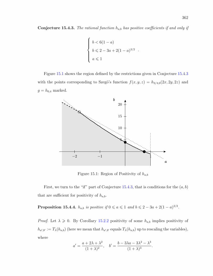
362
Conjecture 15.4.3. The rational function ha,b has positive coefficients if and only if
b < 6(1− a)
b 6 2− 3a+ 2(1− a)3/2
a 6 1
.
Figure 15.1 shows the region defined by the restrictions given in Conjecture 15.4.3
with the points corresponding to Szego’s function f(x, y, z) = h3/4,0(2x, 2y, 2z) and
g = h0,4 marked.
5
10
15
20bb
−2 −1 1
aa
Figure 15.1: Region of Positivity of ha,b
First, we turn to the “if” part of Conjecture 15.4.3, that is conditions for the (a, b)
that are sufficient for positivity of ha,b.
Proposition 15.4.4. ha,b is positive if 0 6 a 6 1 and b 6 2− 3a+ 2(1− a)3/2.
Proof. Let λ > 0. By Corollary 15.2.2 positivity of some ha,b implies positivity of
ha′,b′ := Tλ(ha,b) (here we mean that ha′,b′ equals Tλ(ha,b) up to rescaling the variables),
where
a′ =a+ 2λ+ λ2
(1 + λ)2, b′ =
b− 3λa− 3λ2 − λ3
(1 + λ)3.

363
Starting with the positivity of g = h0,4, that is (a, b) = (0, 4), we find that b′ =
2 − 3a′ + 2(1 − a′)3/2. Using Proposition 15.4.1 this proves the case 0 6 a < 1. For
a = 1 observe that
h1,−1(x, y, z) =1
(1− x)(1− y)(1− z)
is obviously positive.
Using the positivity of g and the positivity preserving operations Tλ we have thus
been able to prove the “if” part of Conjecture 15.4.3 under the hypothesis that a > 0.
Clearly, we can strengthen this hypothesis to a > a1 if we succeed in proving the
positivity of ha1,b1 with b1 = 2− 3a1 + 2(1−a1)3/2. However, according to Conjecture
15.4.3 we neccessarily have a1 > a0, where a0 ≈ −1.81451 is the unique real solution
of
2− 3a0 + 2(1− a0)3/2 = 6(1− a0).
Let’s now consider the “only if” direction of Conjecture 15.4.3.
Proposition 15.4.5. ha,b is positive only if b < 6(1− a) and a 6 1.
Proof. Observe that the coefficient of xyz in the expansion of ha,b(x, y, z) evaluates
as 6(1− a)− b which proves that b < 6(1− a) for positivity.
For the second claim we expand ha,b(x, y, 0) as
ha,b(x, y, 0) =1
1− x− y + axy=∑n>0
(1− ax)n
(1− x)n+1yn.
Using
1
(1− x)n+1=∑m>0
(n+m
n
)xm,
we deduce that the coefficient of xyn in ha,b(x, y, z) is given by n+ 1− na. Positivity
of ha,b thus implies that
a <n+ 1
n

364
for all positive integers n.
Proposition 15.4.4 is based upon the positivity of g = h0,4, which by Proposition
15.4.1 implies that b 6 4 suffices for positivity of h0,b. This bound turns out to be
sharp.
Proposition 15.4.6. h0,b is positive only if b 6 4.
Proof. We expand h0,b as
h0,b(x, y, z) =1
1− x− y − z + bxyz=∑n>0
(1− bxy)n
(1− x− y)n+1zn.
Using
1
(1− x− y)n+1=∑m>0
(n+m
n
)(x+ y)m,
we conclude that the coefficient of xynzn in h0,b(x, y, z) is given by
(n+ 1)
(2n+ 1
n
)− bn
(2n− 1
n
).
Positivity of h0,b then implies that
b <2(2n+ 1)
n
for all integers n > 0.
Corollary 15.4.7. Let a 6 0. Then ha,b is positive only if b 6 2− 3a+ 2(1− a)3/2.
Proof. Otherwise an application of Tλ with appropriate λ > 0 would produce (after
normalization) a positive h0,b′ with b′ > 4 contradicting Proposition 15.4.6.
To improve on the hypothesis a 6 0, it would be desirable to show optimality
of Szego’s function, that is that ha,0 is positive only if a 6 3/4. As in the proof of

365
Proposition 15.4.6 we believe that it suffices to consider the coefficients of xynzn in
ha,0(x, y, z). While we readily find a second order recurrence for those coefficients we
didn’t see how to derive the necessity of a 6 3/4 in order to prove positivity.
Example 15.4.8. By computing the first 100 coefficients of xynzn in ha,0(x, y, z) we
learn that ha,0 is positive only if a < 0.75188.
The (conjectured) optimality of Szego’s function f is surprising in this context
since f = T1(g) allows us to conclude the positivity of f from the positivity of g
but not vice versa. Yet, the positivity preserving operator T1 still provided us with
an optimal result. In fact, more seems to be true. As stated in Conjecture 15.4.3,
starting with a positive ha,b which is optimal (in the sense that increasing either a
or b will destroy positivity) the positivity preserving operators Tλ, λ > 0, not only
yield a positive rational function Tλ(ha,b) but again they seem to produce an optimal
rational function.

366
Chapter 16
A q-analog of Ljunggren’s binomialcongruence
The contents of this chapter (apart from minor corrections or adaptions) have
been published as:
[Str11] A q-analog of Ljunggren’s binomial congruencepublished in DMTCS Proceedings: 23rd International Conference on Formal Power Series
and Algebraic Combinatorics (FPSAC), Jun 2011, p. 897-902
Abstract We prove a q-analog of a classical binomial congruence due to Ljunggren
which states that (ap
bp
)≡(a
b
)modulo p3 for primes p > 5. This congruence subsumes and builds on earlier congru-
ences by Babbage, Wolstenholme and Glaisher for which we recall existing q-analogs.
Our congruence generalizes an earlier result of Clark.
16.1 Introduction and notation
Recently, q-analogs of classical congruences have been studied by several authors
including [Cla95], [And99], [SP07], [Pan07], [CP08], [Dil08]. Here, we consider the
classical congruence (ap
bp
)≡(a
b
)mod p3 (16.1)

367
which holds true for primes p > 5. This also appears as Problem 1.6 (d) in [Sta97].
Congruence (16.1) was proved in 1952 by Ljunggren, see [Gra97], and subsequently
generalized by Jacobsthal, see Remark 16.4.2.
Let [n]q := 1 + q + . . . qn−1, [n]q! := [n]q[n− 1]q · · · [1]q and
(n
k
)q
:=[n]q!
[k]q![n− k]q!
denote the usual q-analogs of numbers, factorials and binomial coefficients respec-
tively. Observe that [n]1 = n so that in the case q = 1 we recover the usual factorials
and binomial coefficients as well. Also, recall that the q-binomial coefficients are poly-
nomials in q with nonnegative integer coefficients. An introduction to these q-analogs
can be found in [Sta97].
We establish the following q-analog of (16.1):
Theorem 16.1.1. For primes p > 5 and nonnegative integers a, b,
(ap
bp
)q
≡(a
b
)qp2−(
a
b+ 1
)(b+ 1
2
)p2 − 1
12(qp − 1)2 mod [p]3q. (16.2)
The congruence (16.2) and similar ones to follow are to be understood over the
ring of polynomials in q with integer coefficients. We remark that p2 − 1 is divisible
by 12 for all primes p > 5.
Observe that (16.2) is indeed a q-analog of (16.1): as q → 1 we recover (16.1).
Example 16.1.2. Choosing p = 13, a = 2, and b = 1, we have
(26
13
)q
= 1 + q169 − 14(q13 − 1)2 + (1 + q + . . .+ q12)3f(q)
where f(q) = 14 − 41q + 41q2 − . . . + q132 is an irreducible polynomial with integer
coefficients. Upon setting q = 1, we obtain(
2613
)≡ 2 modulo 133.
368
Since our treatment very much parallels the classical case, we give a brief history
of the congruence (16.1) in the next section before turning to the proof of Theorem
16.1.1.
16.2 A bit of history
A classical result of Wilson states that (n − 1)! + 1 is divisible by n if and only
if n is a prime number. “In attempting to discover some analogous expression which
should be divisible by n2, whenever n is a prime, but not divisible if n is a composite
number”, [Bab19], Babbage is led to the congruence
(2p− 1
p− 1
)≡ 1 mod p2 (16.3)
for primes p > 3. In 1862 Wolstenholme, [Wol62], discovered (16.3) to hold modulo
p3, “for several cases, in testing numerically a result of certain investigations, and
after some trouble succeeded in proving it to hold universally” for p > 5. To this end,
he proves the fractional congruences
p−1∑i=1
1
i≡ 0 mod p2, (16.4)
p−1∑i=1
1
i2≡ 0 mod p (16.5)
for primes p > 5. Using (16.4) and (16.5) he then extends Babbage’s congruence
(16.3) to hold modulo p3: (2p− 1
p− 1
)≡ 1 mod p3 (16.6)
for all primes p > 5. Note that (16.6) can be rewritten as(
2pp
)≡ 2 modulo p3.
The further generalization of (16.6) to (16.1), according to [Gra97], was found by

369
Ljunggren in 1952. The case b = 1 of (16.1) was obtained by Glaisher, [Gla00], in
1900.
In fact, Wolstenholme’s congruence (16.6) is central to the further generalization
(16.1). This is just as true when considering the q-analogs of these congruences as we
will see here in Lemma 16.4.1.
A q-analog of the congruence of Babbage has been found by Clark [Cla95] who
proved that (ap
bp
)q
≡(a
b
)qp2
mod [p]2q. (16.7)
We generalize this congruence to obtain the q-analog (16.2) of Ljunggren’s congruence
(16.1). A result similar to (16.7) has also been given by Andrews in [And99].
Our proof of the q-analog proceeds very closely to the history just outlined. Be-
sides the q-analog (16.7) of Babbage’s congruence (16.3) we will employ q-analogs of
Wolstenholme’s harmonic congruences (16.4) and (16.5) which were recently supplied
by Shi and Pan, [SP07]:
Theorem 16.2.1. For primes p > 5,
p−1∑i=1
1
[i]q≡ −p− 1
2(q − 1) +
p2 − 1
24(q − 1)2[p]q mod [p]2q (16.8)
as well asp−1∑i=1
1
[i]2q≡ −(p− 1)(p− 5)
12(q − 1)2 mod [p]q. (16.9)
This generalizes an earlier result [And99] of Andrews.
16.3 A q-analog of Ljunggren’s congruence
In the classical case, the typical proof of Ljunggren’s congruence (16.1) starts with
the Chu-Vandermonde identity which has the following well-known q-analog:

370
Theorem 16.3.1.
(m+ n
k
)q
=∑j
(m
j
)q
(n
k − j
)q
qj(n−k+j).
We are now in a position to prove the q-analog of (16.1).
Proof of Theorem 16.1.1. As in [Cla95] we start with the identity
(ap
bp
)q
=∑
c1+...+ca=bp
(p
c1
)q
(p
c2
)q
· · ·(p
ca
)q
qp∑
16i6a(i−1)ci−∑
16i<j6a cicj(16.10)
which follows inductively from the q-analog of the Chu-Vandermonde identity given
in Theorem 16.3.1. The summands which are not divisible by [p]2q correspond to the
ci taking only the values 0 and p. Since each such summand is determined by the
indices 1 6 j1 < j2 < . . . < jb 6 a for which ci = p, the total contribution of these
terms is
∑16j1<...<jb6a
qp2∑bk=1(jk−1)−p2(b2) =
∑06i16...6ib6a−b
qp2∑bk=1 ik =
(a
b
)qp2.
This completes the proof of (16.7) given in [Cla95].
To obtain (16.2) we now consider those summands in (16.10) which are divisible
by [p]2q but not divisible by [p]3q. These correspond to all but two of the ci taking
values 0 or p. More precisely, such a summand is determined by indices 1 6 j1 <
j2 < . . . < jb < jb+1 6 a, two subindices 1 6 k < ` 6 b + 1, and 1 6 d 6 p − 1 such
that
ci =
d for i = jk,
p− d for i = j`,
p for i ∈ {j1, . . . , jb+1}\{jk, j`},
0 for i 6∈ {j1, . . . , jb+1}.

371
For each fixed choice of the ji and k, ` the contribution of the corresponding summands
isp−1∑d=1
(p
d
)q
(p
p− d
)q
qp∑
16i6a(i−1)ci−∑
16i<j6a cicj
which, using that qp ≡ 1 modulo [p]q, reduces modulo [p]3q to
p−1∑d=1
(p
d
)q
(p
p− d
)q
qd2
=
(2p
p
)q
− [2]qp2 .
We conclude that
(ap
bp
)q
≡(a
b
)qp2
+
(a
b+ 1
)(b+ 1
2
)((2p
p
)q
− [2]qp2
)mod [p]3q. (16.11)
The general result therefore follows from the special case a = 2, b = 1 which is
separately proved next.
16.4 A q-analog of Wolstenholme’s congruence
We have thus shown that, as in the classical case, the congruence (16.2) can be
reduced, via (16.11), to the case a = 2, b = 1. The next result therefore is a q-analog
of Wolstenholme’s congruence (16.6).
Lemma 16.4.1. For primes p > 5,
(2p
p
)q
≡ [2]qp2 −p2 − 1
12(qp − 1)2 mod [p]3q.
Proof. Using that [an]q = [a]qn [n]q and [n+m]q = [n]q + qn [m]q we compute
(2p
p
)q
=[2p]q [2p− 1]q · · · [p+ 1]q
[p]q [p− 1]q · · · [1]q=
[2]qp
[p− 1]q!
p−1∏k=1
([p]q + qp [p− k]q
)

372
which modulo [p]3q reduces to (note that [p− 1]q! is relatively prime to [p]3q)
[2]qp
(q(p−1)p + q(p−2)p
∑16i6p−1
[p]q[i]q
+ q(p−3)p∑
16i<j6p−1
[p]q [p]q[i]q [j]q
). (16.12)
Combining the results (16.8) and (16.9) of Shi and Pan, [SP07], given in Theorem
16.2.1, we deduce that for primes p > 5,
∑16i<j6p−1
1
[i]q [j]q≡ (p− 1)(p− 2)
6(q − 1)2 mod [p]q. (16.13)
Together with (16.8) this allows us to rewrite (16.12) modulo [p]3q as
[2]qp
(q(p−1)p + q(p−2)p
(−p− 1
2(qp − 1) +
p2 − 1
24(qp − 1)2
)+
+q(p−3)p (p− 1)(p− 2)
6(qp − 1)2
).
Using the binomial expansion
qmp = ((qp − 1) + 1)m =∑k
(m
k
)(qp − 1)k
to reduce the terms qmp as well as [2]qp = 1 + qp modulo the appropriate power of [p]q
we obtain
(2p
p
)q
≡ 2 + p(qp − 1) +(p− 1)(5p− 1)
12(qp − 1)2 mod [p]3q.
Since
[2]qp2 ≡ 2 + p(qp − 1) +(p− 1)p
2(qp − 1)2 mod [p]3q
the result follows.
Remark 16.4.2. Jacobsthal, see [Gra97], generalized the congruence (16.1) to hold

373
modulo p3+r where r is the p-adic valuation of
ab(a− b)(a
b
)= 2a
(a
b+ 1
)(b+ 1
2
).
It would be interesting to see if this generalization has a nice analog in the q-world.
374
Chapter 17
Outlook
In the following two final sections we comment on certain aspects of two methods
which have been in repeated use throughout this thesis: the method of brackets and
the method of creative telescoping. We demonstrate how, at least in each particular
instance, the method of brackets can be made rigorous by translating its application
into the framework of Mellin–Barnes contour integrals. Finally we describe a situaton
in which a direct application of creative telescoping is prevented by the divergence
of the involved integrals. It is pointed out that, on the level of Mellin calculus, the
difficulties at hand can be dealt with by considering distributions instead of classical
functions. For both methods this indicates opportunities for further investigation.
17.1 The method of brackets and similar
approaches
The method of brackets has been discussed in Chapters 8 and 9. In particular, it
was shown that it can be regarded as a multi-dimensional extension of Ramanujan’s
Master Theorem in the form
∫ ∞0
xs−1
[∞∑n=0
(−1)n
n!λ(n)xn
]dx = Γ(s)λ(−s). (17.1)
375
In Section 17.1.1 below, we briefly sketch the negative dimensional integration
(NDIM) approach [HR87] which led [GS07] to the method of brackets, initially re-
ferred to as optimized NDIM. While the fundamental (formal) objects in NDIM are
the integrals ∫ ∞−∞
(x2)α dDx,
a very natural choice in the context of the evaluation of Feynman integrals, the
method of brackets revolves around the (formal) integrals
∫ ∞0
xα−1 dx,
which are usually more convenient for the evaluation of general definite integrals as
collected, for instance, in [GR80].
In Section 17.1.2 we describe, mostly by example, how an application of the
method of brackets can be made rigorous by writing the integrand in terms of Mellin–
Barnes contour integrals which is a common practice in the context of evaluating
Feynman integrals [Smi06]. The heuristic part of the method of brackets is Rule 8.9.3
which postulates that an integral is evaluated as the joint contribution of the sum-
mations (each corresponding to a choice of free variables) converging in a common
region. As will become clear, this situation corresponds to a representation of the
desired integral as a multiple Mellin–Barnes integral: closing the contours in a par-
ticular way and collecting the appropriate residues yields a series which gives the
integral in its region of convergence. For future investigations, it would be interesting
to make the relation between combinations of free variables and collections of residues
more explicit. Further, given a multiple Mellin–Barnes integral
1
(2πi)n
∫ c1+i∞
c1−i∞· · ·∫ cn+i∞
cn−i∞
∏rk=1 Γ(Lk(s1, . . . , sn))∏sk=r+1 Γ(Lk(s1, . . . , sn))
x−s11 · · ·x−snn ds1 · · · dsn, (17.2)
376
where the Lk are affine, it would be useful to have a systematic way of determining
appropriate sets of residues whose sum represents (17.2) in a chosen region. For n = 2
this problem is discussed in [FG12].
17.1.1 Negative dimensional integration
In the negative dimensional integration (NDIM) approach, advocated in [HR87],
one makes the formal definition
∫ ∞−∞
(x2)α dDx = (−1)απD/2Γ(α + 1) δα+D/2,0. (17.3)
Here, x = (x1, . . . , xD), x2 = x21 + . . .+x2
D and δi,j is the Kronecker delta. This formal
identity is used for nonnegative α and gives a non-zero value only when the D 6 0,
which explains the label of negative dimensionality.
Initially, α is a positive integer and the definition (17.3) is motivated by taking
the limit β → 0 of
∫ ∞−∞
(x2)α
(x2 +M2)βdDx = πD/2(M2)D/2+α−βΓ(α +D/2)Γ(β − α−D/2)
Γ(D/2)Γ(β). (17.4)
It is then observed in [HR87] that, using the formal rule (17.3), the Gaussian
integral evaluates as
∫ ∞−∞
e−αx2
dDx =∑n
(−α)n
n!
∫ ∞−∞
(x2)ndDx (17.5)
=∑n
(−α)n
n!(−1)nπD/2Γ(n+ 1) δn+D/2,0
=(πα
)D/2.

377
In turn, the formal equality
∑n
(−α)n
n!
∫ ∞−∞
(x2)ndDx =(πα
)D/2may be used to motivate the definition (17.3).
The method of brackets, as first presented in [GS07], started from the same under-
lying idea. Instead of formally expanding the Gaussian integral (17.5), one expands
Γ(s)
αs=
∫ ∞0
xs−1e−αx dx =∑n
(−α)n
n!
∫ ∞0
xn+s−1 dx,
which leads to the formal definition [GS07, (A.2)]
∫ ∞0
xn+s−1 dx =Γ(s)Γ(n+ 1)
(−1)nδn+s,0. (17.6)
Gonzalez and Schmidt then introduce the notation 〈n+ s〉 for the left-hand side and
go on to develop the formal rules that are presented in Section 8.9 of Chapter 8.
One advantage of the modified approach (17.6) over the original (17.3) is that it
is easier to apply to integrals outside the context of Feynman integrals. A variety of
examples is given in [GM10].
17.1.2 Mellin–Barnes integrals
Another standard practice, especially in particle physics [Smi06], is the intro-
duction of Mellin–Barnes representations to evaluate definite integrals. The final
(multiple) Mellin–Barnes integral may then be solved by closing the contours and
collecting the appropriate residues. By way of several examples, we will illustrate
that an application of the method of brackets corresponds to a way of systematically
introducing Mellin–Barnes representations. The rigor that may be obtained in this

378
fashion comes at the price of introducing, along the way, arguably more technically
involved contour integrals and having to collect appropriate sets of residues.
We begin by illustrating the correspondence by observing that a Taylor expan-
sion of a function f(x) may be expressed as a Mellin–Barnes integral representation.
Namely, if
f(x) =∞∑n=0
(−1)n
n!a(n)xn, (17.7)
then, by Ramanujan’s Master Theorem and under appropriate conditions on a(n) as
stated for instance in Theorem 8.3.2, we have
∫ ∞0
xs−1f(x) dx = Γ(s)a(−s). (17.8)
Hence, by Mellin inversion, proved in Theorem 17.1.6, f(x) has the Mellin–Barnes
integral representation
f(x) =1
2πi
∫ i∞
−i∞Γ(s)a(−s)x−s ds. (17.9)
Here, and below, the exact contour is meant to be chosen appropriately. In this case
that means that the poles of Γ(s) lie to the left of the contour and that, on this side,
a(−s) is analytic.
Example 17.1.1. In the case f(x) = 11+x
we have a(n) = Γ(n+ 1) and hence
1
1 + x=
1
2πi
∫ i∞
−i∞Γ(s)Γ(1− s)x−s ds. (17.10)
We remark that closing the contour to the left reproduces the Taylor expansion of
f(x) at 0 which converges for |x| < 1. The Mellin–Barnes representation of f(x) also
allows the contour to be closed to the right. In that case, one sums the residues at

379
the poles s = n+ 1 for n = 0, 1, . . . to obtain the series
∞∑n=0
(−1)n
n!Γ(n+ 1)x−(n+1) =
1
x
1
1 + 1x
=1
1 + x,
which also represents f(x), but now for |x| > 1. It is this well-known aspect of Mellin–
Barnes representations [AAR99] that is responsible for the fact that the method of
brackets is able to give different evaluations of a given integral which are valid in
different regions and analytic continuations of each other.
The bracket expansion
1
(a1 + a2)α=∑m1,m2
(−1)m1+m2
m1!m2!am1
1 am22
〈α +m1 +m2〉Γ(α)
(17.11)
stated more generally as Rule 8.9.1 has the following Mellin–Barnes analog:
1
(a1 + a2)α=
1
2πi
∫ i∞
−i∞
Γ(−s)Γ(α + s)
Γ(α)as1a
−α−s2 ds (17.12)
Here, | arg a1− arg a2| < π and the contour is understood to be such that it separates
the poles s = 0, 1, 2, . . . of Γ(−s) from the poles s = −α,−α− 1, . . . of Γ(α + s).
Remark 17.1.2. Equation (17.12) is a special case of the Mellin–Barnes representa-
tion, see [PK01, Section 3.4.2], for the hypergeometric function, valid for | arg(x)| < π,
Γ(a)Γ(b)
Γ(c)2F1
(a, b
c
∣∣∣∣−x) =1
2πi
∫ i∞
−i∞
Γ(a+ s)Γ(b+ s)
Γ(c+ s)Γ(−s)xs ds,
and the fact that, when b = c, the left-hand side reduces to Γ(a)(1+x)a
.
In a sequence of examples we now show how these tools, coupled with the inverse
Mellin transform which is shortly reviewed in Section 17.1.3, allow evaluation of
definite integrals along the lines of an application of the method of brackets.
380
Example 17.1.3. As in Section 8.9.1 we consider, for illustration, the integral
∫ ∞0
∫ ∞0
xs−1yt−1 exp (−(x+ y)α) dx dy.
Using the Mellin–Barnes integral (17.9) for the exponential function, followed by an
application of (17.12), we have
exp (−(x+ y)α) =1
2πi
∫ i∞
−i∞Γ(σ)(x+ y)−σα dσ
=1
(2πi)2
∫ i∞
−i∞
∫ i∞
−i∞
Γ(σ)Γ(−τ)Γ(σα + τ)
Γ(σα)xτy−σα−τ dτ dσ
=1
(2πi)2
∫ i∞
−i∞
∫ i∞
−i∞
1
α
Γ( s+tα
)Γ(s)Γ(t)
Γ(s+ t)x−sy−t ds dt.
In the last step we performed the change of variables −s = τ and −t = −σα−τ . Thus
an application of the (multiple) inverse Mellin transform, stated as Theorem 17.1.6,
yields the integral evaluation
∫ ∞0
∫ ∞0
xs−1yt−1 exp (−(x+ y)α) dx dy =1
α
Γ( s+tα
)Γ(s)Γ(t)
Γ(s+ t).
This agrees with the result obtained in Section 8.9.1 using the method of brackets.
Example 17.1.4. Consider, for α, β, ν > 0, the integral
∫ ∞0
xνe−αxJν(βx) dx =(2β)νΓ(ν + 1
2)√
π(α2 + β2)ν+1/2(17.13)
that was evaluated in Section 9.3 using the method of brackets. The relevant Mellin–
Barnes representations, equivalent through (17.9) to the respective Taylor expansions,
381
are
e−αx =1
2πi
∫ i∞
−i∞
Γ(s)
αsx−s ds,
xνJν(βx) =1
2πi
∫ i∞
−i∞
1
2
(2
β
)t+ν Γ(ν + t2)
Γ(1− t2)x−t dt,
valid for Re s > 0 and −2ν < Re t < 3/2 − ν, respectively. Recall that the contour
integrals are understood to seperate the increasing from the decreasing sequence of
poles.
After the change of variables u = s+ t, v = t/2, we have
e−αxxνJν(βx) =1
(2πi)2
∫ i∞
−i∞
∫ i∞
−i∞
Γ(u− 2v)
αu−2v
(2
β
)2v+νΓ(ν + v)
Γ(1− v)x−u dv du.
It then follows that the left-hand side of (17.13) is given by setting u = 1 in
∫ ∞0
xu+ν−1e−αxJν(βx) dx =1
2πi
∫ i∞
−i∞
Γ(u− 2v)
αu−2v
(2
β
)2v+νΓ(ν + v)
Γ(1− v)dv. (17.14)
Note that the integrand has two sequences of poles: an increasing sequence of poles at
2v = u, u+1, u+2, . . . and a decreasing sequence of poles at v = −ν,−ν−1,−ν−2, . . ..
Closing the contour to the left, that is collecting the residues of the poles at v = −ν−n
for n ∈ Z>0, yields
1
αu+ν
∞∑n=0
(−1)n
n!
Γ(u+ 2ν + 2n)
Γ(1 + ν + n)
(β
2α
)ν+2n
.
In the case u = 1 this is precisely the series (9.12) obtained previously by the method
of brackets. In particular, one obtains, for |β| < |α|, the evaluation (17.13).
On the other hand, closing the contour in (17.14) to the right, yields the series
1
2
(2
β
)u+ν ∞∑n=0
(−1)n
n!
(2α
β
)nΓ(ν + u/2 + n/2)
Γ(1− u/2− n/2),

382
which, for u = 1, coincides with (9.14). This second series converges for |β| > |α|.
Example 17.1.5. In this example we will illustrate the heuristic Rule 8.9.3 of the
method of brackets by evaluating the integral
∫ ∞0
J0(αx)xs−1
(1 + x2)λdx, (17.15)
first by employing the method of brackets and then, in the corresponding fashion, by
the Mellin–Barnes approach. For this integral, the method of brackets yields three
bracket series, one of which is divergent. The two other series converge in a common
region and add up to (17.15). This is confirmed in the Mellin–Barnes approach which
results in a Mellin–Barnes contour integral representing (17.15): closing the contour
to the right produces a divergent asymptotic expansion while closing the contour to
the left results in two series of residues which together give (17.15).
Applying the method of brackets, we have
∫ ∞0
J0(αx)xs−1
(1 + x2)λdx
=∑k
φk
∫ ∞0
(α2
)2k 1
Γ(k + 1)
x2k+s−1
(1 + x2)λdx
=1
Γ(λ)
∑k,n,m
φk,n,m
(α2
)2k 1
Γ(k + 1)〈n+m+ λ〉 〈2m+ 2k + s〉 .
There are 3 indices and 2 brackets which leaves 1 free variable to be chosen. If k is
chosen as the free variable, then m∗ = −k− s2
and n∗ = −λ+ k+ s2. Since | det | = 2,

383
the contribution is
1
2Γ(λ)
∑k
φk
(α2
)2k 1
Γ(k + 1)Γ(−n∗)Γ(−m∗) (17.16)
=1
2Γ(λ)
∑k
(−1)k
(k!)2
(α2
)2k
Γ(λ− k − s2)Γ(k + s
2)
=Γ( s
2)Γ(λ− s
2)
2Γ(λ)1F2
(s2
1, 1− λ+ s2
∣∣∣∣α2
4
).
This converges for∣∣∣α2
4
∣∣∣ < 1. Similarly, the contribution with n as the free variable is
(α2
)2λ−s Γ(−λ+ s2)
2Γ(λ+ 1− s2)
1F2
(λ
1 + λ− s2, 1 + λ− s
2
∣∣∣∣α2
4
), (17.17)
which converges in the same region. On the other hand, with m as free variable one
obtains the divergent series
1
2Γ(λ)
∑m
(−1)m
m!
(α2
)−2m−s Γ(m+ λ)Γ(m+ s2)
Γ(1−m− s2)
. (17.18)
Combining the two convergent series, we therefore have the evaluation
∫ ∞0
J0(αx)xs−1
(1 + x2)λdx =
Γ( s2)Γ(λ− s
2)
2Γ(λ)1F2
(s2
1, 1− λ+ s2
∣∣∣∣α2
4
)+(α
2
)2λ−s Γ(−λ+ s2)
2Γ(λ+ 1− s2)
1F2
(λ
1 + λ− s2, 1 + λ− s
2
∣∣∣∣α2
4
).
We remark that in the special case s = 2 this combines pleasantly to
∫ ∞0
J0(αx)x
(1 + x2)λ+1dx =
(α2
)λ Kλ(α)
λ!,
and, even more specially,
∫ ∞0
J0(αx)x
(1 + x2)3/2dx = e−α.

384
Let us now evaluate (17.15) by using the Mellin–Barnes approach. In that case we
commence with
J0(αx) =1
2πi
∫ i∞
−i∞
1
2
(2
α
)sΓ(s/2)
Γ(1− s/2)x−s ds
which, as in (17.9), is equivalent to the series expansion of J0(αx). By (17.12),
introduced as the analog of Rule 8.9.1, we further have
1
(1 + x2)λ=
1
2πi
∫ i∞
−i∞
Γ(−t)Γ(λ+ t)
Γ(λ)x2t dt.
Hence, after the change of variables u = s− 2t,
J0(αx)
(1 + x2)λ=
1
2πi
∫ i∞
−i∞
[1
2πi
∫ i∞
−i∞
1
2
(2
α
)u+2tΓ(u/2 + t)Γ(−t)Γ(λ+ t)
Γ(1− u/2− t)Γ(λ)dt
]x−u du.
By the Mellin inversion formula, Theorem 17.1.6, it follows that
∫ ∞0
J0(αx)xs−1
(1 + x2)λdx =
1
2πi
∫ i∞
−i∞
1
2
(2
α
)s+2tΓ(s/2 + t)Γ(−t)Γ(λ+ t)
Γ(1− s/2− t)Γ(λ)dt.
(17.19)
The integrand has decreasing sequences of poles at t = −s/2− n and t = −λ− n for
n ∈ Z>0. The residues of the poles at t = −s/2− n sum to
1
2
∞∑n=0
(−1)n
n!
(α2
)2n Γ(s/2 + n)Γ(λ− s/2− n)
Γ(1 + n)Γ(λ), (17.20)
which coincides with (17.16). Likewise the residues of the poles at t = −λ − n sum
to
1
2
∞∑n=0
(−1)n
n!
(α2
)2n+2λ−s Γ(λ+ n)Γ(s/2− λ− n)
Γ(1− s/2 + λ+ n)Γ(λ), (17.21)
which rewrites to (17.17). If, on the other hand, one closes the contour in (17.19) to
the right then the residues at t = 0, 1, 2, . . . yield the divergent asymptotic expansion

385
(17.18).
17.1.3 Mellin transform
For completeness and convenience of the reader we include here a proof of the
Mellin inversion theorem which is at the heart of Section 17.1.2. The proof given here
is adopted from the two-dimensional case discussed in [Ree44, Fox57] which is based
on Mellin’s original treatment; it thus is most likely precisely the classical one.
Theorem 17.1.6 (Mellin inversion formula). Assume that F (s) is analytic in the
strip a < Re s < b and that F (s) → 0 as | Im s| → ∞. upon restricting to compact
[a’,b’]) Define f by
f(x) =1
2πi
∫ c+i∞
c−i∞F (s)x−s ds. (17.22)
If this integral converges absolutely for all c ∈ (a, b), then
F (s) =
∫ ∞0
xs−1f(x) dx.
Proof. First, note that the integral (17.22) does not depend on the specific value of
c ∈ (a, b). Given s with a < Re s < b we can therefore write, for any c1, c2 satisfying
a < c1 < Re s < c2 < b,
∫ ∞0
xs−1f(x) dx =
∫ 1
0
xs−1 1
2πi
∫ c1+i∞
c1−i∞F (t)x−t dt dx
+
∫ ∞1
xs−1 1
2πi
∫ c2+i∞
c2−i∞F (t)x−t dt dx
= − 1
2πi
∫ c1+i∞
c1−i∞
F (t)
t− s dt+1
2πi
∫ c2+i∞
c2−i∞
F (t)
t− s dt,
where in the last step we used that the involved integrals are absolutely convergent
to justify switching the order of integration. By Cauchy’s residue theorem we have,

386
for M > | Im s|,
1
2πi
[∫ c2+iM
c2−iM−∫ c2+iM
c1+iM
−∫ c1+iM
c1−iM+
∫ c2−iM
c1−iM
]F (t)
t− s dt = F (s).
By the assumed convergence F (t) → 0 as | Im t| → ∞, the two auxiliary horizontal
line integrals vanish as M →∞. Hence
∫ ∞0
xs−1f(x) dx = F (s)
as claimed.
The Mellin inversion theorem and its proof extend to several variables. The two-
dimensional case, which results in no loss of generality, is proven in [Ree44] along the
lines of the proof just given.
Theorem 17.1.7. Assume that F (s1, . . . , sn), as a function of sk, is analytic in the
strip ak < Re sk < bk for each k = 1, . . . , n. Further, assume that F (s1, . . . , sn)→ 0
as | Im s1|, . . . , | Im sn| → ∞, independently of each other. Define f by
f(x1, . . . , xn) =1
(2πi)n
∫ c1+i∞
c1−i∞· · ·∫ cn+i∞
cn−i∞F (s1, . . . , sn)x−s11 · · ·x−snn ds1 · · · dsn.
(17.23)
If this integral converges absolutely for all c1, . . . , cn with ck ∈ (ak, bk) then
F (s1, . . . , sn) =
∫ ∞0
· · ·∫ ∞
0
xs1−11 · · ·xsn−1
n f(x1, . . . , xn) dx1 · · · dxn.
387
17.2 Creative telescoping leading to divergent
integrals
In this section, we apply the creative telescoping approach to the problem, consid-
ered in Chapter 4, of obtaining the differential equation satisfied by the probability
density function p4. This problem splits into two parts: finding the differential equa-
tion and proving that p4 is one of its solutions. As we are going to illustrate, the
first part of this problem is straightforward to solve using creative telescoping. Yet,
the step of proving, which in other applications of creative telescoping often reduces
to routine verification, poses certain issues, described below, which include that ap-
plying differential operators and taking limits do not commute. We do not offer a
satisfactory resolution but remark that a general approach to solving the issues at
hand would be interesting: when deducing the differential equation in Chapter 4 we
had to use the distributional Mellin transform to work around the issues.
The probability density of the distance travelled by a four-step random walk, as
discussed in Chapter 4, is
p4(x) =
∫ ∞0
xtJ0(t)4J0(xt) dt, (17.24)
where J0 is a Bessel function. Using Mellin calculus and the relation of p4 to the mo-
ments W4, it was shown in Example 4.2.3 of Chapter 4 that p4 satisfies the differential
equation A4 · p4 = 0 with
A4 = x4(θ + 1)3 − 4x2θ(5θ2 + 3) + 64(θ − 1)3 (17.25)
= (x− 4)(x− 2)x3(x+ 2)(x+ 4)D3x + 6x4
(x2 − 10
)D2x
+ x(7x4 − 32x2 + 64
)Dx +
(x2 − 8
) (x2 + 8
).
Here θ = xDx = x ddx
.
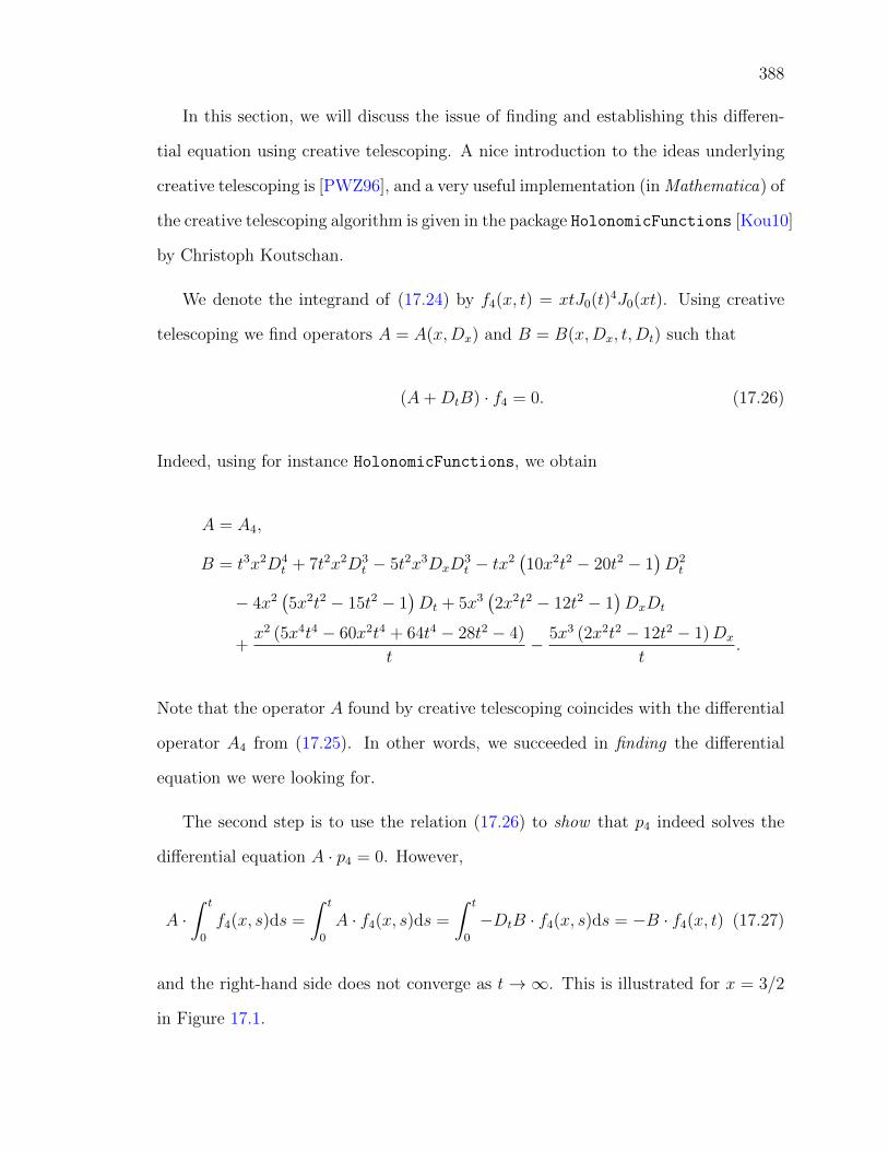
388
In this section, we will discuss the issue of finding and establishing this differen-
tial equation using creative telescoping. A nice introduction to the ideas underlying
creative telescoping is [PWZ96], and a very useful implementation (in Mathematica) of
the creative telescoping algorithm is given in the package HolonomicFunctions [Kou10]
by Christoph Koutschan.
We denote the integrand of (17.24) by f4(x, t) = xtJ0(t)4J0(xt). Using creative
telescoping we find operators A = A(x,Dx) and B = B(x,Dx, t, Dt) such that
(A+DtB) · f4 = 0. (17.26)
Indeed, using for instance HolonomicFunctions, we obtain
A = A4,
B = t3x2D4t + 7t2x2D3
t − 5t2x3DxD3t − tx2
(10x2t2 − 20t2 − 1
)D2t
− 4x2(5x2t2 − 15t2 − 1
)Dt + 5x3
(2x2t2 − 12t2 − 1
)DxDt
+x2 (5x4t4 − 60x2t4 + 64t4 − 28t2 − 4)
t− 5x3 (2x2t2 − 12t2 − 1)Dx
t.
Note that the operator A found by creative telescoping coincides with the differential
operator A4 from (17.25). In other words, we succeeded in finding the differential
equation we were looking for.
The second step is to use the relation (17.26) to show that p4 indeed solves the
differential equation A · p4 = 0. However,
A ·∫ t
0
f4(x, s)ds =
∫ t
0
A · f4(x, s)ds =
∫ t
0
−DtB · f4(x, s)ds = −B · f4(x, t) (17.27)
and the right-hand side does not converge as t→∞. This is illustrated for x = 3/2
in Figure 17.1.

389
120 140 160 180 200
-40 000
-20 000
20 000
40 000
Figure 17.1: −B · f4(3/2, t)
In fact, it is not true that, as t→∞,
Dnx ·∫ t
0
f4(x, s)ds −→ Dnx ·∫ ∞
0
f4(x, s)ds = p(n)4 (x). (17.28)
To see the failure of (17.28), note that in the case n = 2
D2x ·∫ t
0
f4(x, s)ds =
∫ t
0
D2x · f4(x, s)ds = −
∫ t
0
s2J0(s)4 (xsJ0(xs) + J1(xs)) ds.
(17.29)
In light of the asymptotic form
Jα(x) ≈√
2
πxcos(x− απ
2− π
4
),
the integral (17.29) is seen to not converge as t→∞. The integrand and the integral
are depicted in Figure 17.2.
It is unclear to the author how to proceed from here.
Remark 17.2.1. From (17.27), as suggested by Manuel Kauers, one can proceed by
seeking an operator C = C(x,Dx, t) which annihilates the right-hand side of (17.27).
For such C and for all t > 0, we will then have
CA ·∫ t
0
f4(x, s)ds = 0. (17.30)

390
20 40 60 80 100
-2
-1
1
2
20 40 60 80 100
-2.0
-1.5
-1.0
-0.5
0.5
1.0
1.5
Figure 17.2: The integrand of the RHS of (17.29) and the integral (17.29) whenx = 1/2
Using, for instance, once more the functionality of the package HolonomicFunctions
we indeed find such C of order 10 in Dx and degree 10 in both x and t. Moreover,
the only monomial in C which involves t10 is of the form x10t10; in other words,
C
t10−→ x10 as t→∞.
At this point, we would like to take the limit t → ∞ in (17.30) after dividing both
sides by t10. If possible, this would allow us to conclude that x10A · p4 = 0 which, of
course, implies A · p4 = 0. In light of (17.28), there is, however, similar trouble as in
(17.27): the limit t→∞ in (17.30) can not be taken individually for each monomial
of CA.
Remark 17.2.2. Maybe it is worth pointing out that the integral (17.29) as t→∞
seems to approach the desired value p′′4(x) in a certain “average sense”: as illustrated
in Figure 17.3, the oscillations, though increasing in magnitude, appear to stabilize
about p′′4(x). The same phenomenon can be observed in equation (17.27) and Figure
17.1 where the desired value is zero.
Remark 17.2.3. As suggested by Doron Zeilberger, one way to circumvent the ap-
pearance of integrals that do not converge is to replace the integrand f4(x, t) by
e−λtf4(x, t) with an extra parameter λ > 0. In other words, instead of for p4, as in

391
20 40 60 80 100
-2.0
-1.5
-1.0
-0.5
0.5
1.0
1.5
Figure 17.3: The integral (17.29) when x = 1/2 with p′′4(1/2) = −0.266 superimposed
(17.24), we set out to find a differential equation for
∫ ∞0
xtJ0(t)4J0(xt)e−λt dt. (17.31)
In the resulting equations we finally take the limit λ→ 0.
While this approach can solve the problem of finding and proving a differential
equation for p4, it does so not via the relation (17.26) for the integrand f4(x, t) but
via a corresponding relation for the generalized integrand e−λtf4(x, t). This latter
relation, as well as finding it, is much more involved. It would be nice to deduce, by
some general principle, the differential equation directly from (17.26).
In conclusion, it would be very interesting to have an a priori reason of some
sort that would allow us to conclude (in this and other cases) that the differential
operator A+DtB, from (17.26), found by the creative telescoping method yields the
desired differential operator A annihilating p4 (even though we cannot do the usual
interchange of differentiation and integration). In light of Remark 17.2.2 and the
success of the distributional Mellin transform in this instance, distributions may well
be the right framework for further insight.

392
Bibliography
[AAR99] G. E. Andrews, R. Askey, and R. Roy. Special Functions. CambridgeUniversity Press, 1999.
[AEG+11] T. Amdeberhan, O. Espinosa, I. Gonzalez, M. Harrison, V. H. Moll, andA. Straub. Ramanujan’s Master Theorem. The Ramanujan Journal,2011. Accepted.
[AEMS10] T. Amdeberhan, O. R. Espinosa, V. H. Moll, and A. Straub.Wallis-Ramanujan-Schur-Feynman. American Mathematical Monthly,117(15):618–632, Aug 2010.
[AG72] R. Askey and G. Gasper. Certain rational functions whose power serieshave positive coefficients. Amer. Math. Monthly, 79(4):327–341, apr1972.
[AIK78] R. Askey, M. E. H. Ismail, and T. Koornwinder. Weighted permuta-tion problems and Laguerre polynomials. J. Combin. Theory Ser. A,25(3):277–287, 1978.
[Aka09] H. Akatsuka. Zeta Mahler measures. Journal of Number Theory,129(11):2713–2734, 2009.
[Ali08] I. Aliev. Siegel’s Lemma and sum-distinct sets. Discrete Comput. Geom.,39(1-3):59–66, 2008.
[AM09] T. Amdeberhan and V. Moll. A formula for a quartic integral: a surveyof old proofs and some new ones. The Ramanujan Journal, 18:91–102,2009.
[AMS09] T. Amdeberhan, V. H. Moll, and A. Straub. Closed-form evaluationof integrals appearing in positronium decay. Journal of MathematicalPhysics, 50(10), Oct 2009.
[And99] G. E. Andrews. q-analogs of the binomial coefficient congruences ofBabbage, Wolstenholme and Glaisher. Discrete Math., 204(1):15–25,1999.
[AS72] M. Abramowitz and I. Stegun. Handbook of Mathematical Functionswith Formulas, Graphs and Mathematical Tables. Dover, New York,1972.

393
[Ask74] R. Askey. Certain rational functions whose power series have positivecoefficients. II. SIAM J. Math. Anal., 5(1):53–57, 1974.
[AvEvSZ10] G. Almkvist, C. van Enckevort, D. van Straten, and W. Zudilin. Tablesof Calabi-Yau equations. arXiv:math/0507430v2, 2010.
[Bab19] C. Babbage. Demonstration of a theorem relating to prime numbers.Edinburgh Philosophical J., 1:46–49, 1819.
[Bai32] W. N. Bailey. Some transformations of generalized hypergeometric series,and contour integrals of barnes’s type. Quart. J. Math. Oxford, 3:168–182, 1932.
[Bar64] P. Barrucand. Sur la somme des puissances des coefficients multinomiauxet les puissances successives d’une fonction de Bessel. Comptes rendushebdomadaires des seances de l’Academie des sciences, 258:5318–5320,1964.
[BB91] J. M. Borwein and P. B. Borwein. A cubic counterpart of Jacobi’s iden-tity and the AGM. Transactions of the American Mathematical Society,323(2):691–701, 1991.
[BB98] J. M. Borwein and P. B. Borwein. Pi and the AGM: A Study in AnalyticNumber Theory and Computational Complexity. Wiley, 1998.
[BB01] D. Borwein and J. M. Borwein. Some remarkable properties of sinc andrelated integrals. Ramanujan J., 5:73–90, 2001.
[BB06] J. M. Borwein and D. M. Bradley. Thirty two Goldbach variations. Int.J. Number Theory, 2(1):65–103, 2006.
[BB11] D. Bailey and J. Borwein. Hand-to-hand combat with multi-thousand-digit integrals. Journal of Computational Science, 2011. Web pub-lished Feb 2011, available at: http://www.carma.newcastle.edu.au/
~jb616/combat.pdf.
[BBB97] L. Berggren, J. Borwein, and P. Borwein. Pi: A Source Book. SpringerVerlag, New York, 1997.
[BBB08] R. Baillie, D. Borwein, and J. M. Borwein. Surprising sinc sums andintegrals. American Mathematical Monthly, 115(10):888–901, 2008.
[BBBG08] D. H. Bailey, J. M. Borwein, D. J. Broadhurst, and M. L. Glasser. Ellipticintegral evaluations of Bessel moments and applications. Phys. A: Math.Theor., 41:5203–5231, 2008.
[BBBL01] J. M. Borwein, D. M. Bradley, D. J. Broadhurst, and P. Lisonek. Specialvalues of multiple polylogarithms. Trans. Amer. Math. Soc., 353(3):907–941, 2001.

394
[BBC06] D. H. Bailey, J. M. Borwein, and R. E. Crandall. Integrals of the Isingclass. Jour. Phys. A, 39:12271–12302, 2006.
[BBG94] J. Borwein, P. Borwein, and F. Garvan. Some cubic modular identitiesof ramanujan. Trans. Amer. Math. Soc., 343:35–48, 1994.
[BBG04] J. M. Borwein, D. H. Bailey, and R. Girgensohn. Experimentation inMathematics: Computational Paths to Discovery. A K Peters, 1st edi-tion, 2004.
[BBK01] J. M. Borwein, D. J. Broadhurst, and J. Kamnitzer. Central binomialsums, multiple Clausen values, and zeta values. Experimental Mathe-matics, 10(1):25–34, 2001.
[BBM02] D. Borwein, J. M. Borwein, and B. Mares. Multi-variable sinc integralsand volumes of polyhedra. Ramanujan J., 6:189–208, 2002.
[BBS12] D. Borwein, J. M. Borwein, and A. Straub. A sinc that sank. AmericanMathematical Monthly, 119(7), Aug 2012. (in press).
[BBSW12] D. Borwein, J. M. Borwein, A. Straub, and J. Wan. Log-sine evaluationsof Mahler measures, II. Integers, 2012. (in press).
[BC10] J. M. Borwein and R. E. Crandall. Closed forms: what they are andwhy we care. Notices Amer. Math. Soc., 2010. (in press).
[BCC10] J. M. Borwein, O.-Y. Chan, and R. E. Crandall. Higher-dimensional boxintegrals. Experimental Mathematics, 19(3):431–446, 2010.
[BCGK+10] E. Beyerstedt, N. Cayco-Gajic, N. Kallus, L. Medina, V. Moll, andJ. Stigile. Numerical integration with rational Landen transformations.In preparation, 2010.
[BD91] E. E. Boos and A. I. Davydychev. A method of evaluating massiveFeynman integrals. Theor. Math. Phys., 89:1052–1063, 1991.
[BEM03] G. Boros, O. Espinosa, and V. Moll. On some families of integralssolvable in terms of polygamma and negapolygamma functions. IntegralsTransforms and Special Functions, 14:187–203, 2003.
[Ber85] B. Berndt. Ramanujan’s Notebooks, Part I. Springer-Verlag, New York,1985.
[Ber89] B. Berndt. Ramanujan’s Notebooks, Part II. Springer-Verlag, New York,1989.
[Ber10] O. Bernardi. (Very) short proof of Rayleigh’s Theorem (and extensions).Preprint, 2010.

395
[BG02] D. M. Bradley and R. C. Gupta. On the distribution of the sum of nnon-identically distributed uniform random variables. Ann. Inst. Statist.Math., 54:689–700, 2002.
[BM01] G. Boros and V. Moll. The double square root, Jacobi polynomials andRamanujan’s master theorem. Jour. Comp. Applied Math., 130:337–344,2001.
[BM04] G. Boros and V. Moll. Irresistible Integrals. Cambridge University Press,New York, 1st edition, 2004.
[BNSW11] J. M. Borwein, D. Nuyens, A. Straub, and J. Wan. Some arithmeticproperties of short random walk integrals. The Ramanujan Journal,26(1):109–132, 2011.
[Boy81] D. W. Boyd. Speculations concerning the range of Mahler’s measure.Canad. Math. Bull., 24:453–469, 1981.
[Boy98] D. W. Boyd. Mahler’s measure and special values of L-functions. Ex-periment. Math., 7(1):37–82, 1998.
[Bre99] D. Bressoud. Proofs and Confirmations: the story of the AlternatingSign Matrix Conjecture. Cambridge University Press, 1999.
[Bro09] D. J. Broadhurst. Bessel moments, random walks and Calabi-Yau equa-tions. Preprint, 2009.
[BS08] J. M. Borwein and B. Salvy. A proof of a recursion for Bessel moments.Experimental Mathematics, 17:223–230, 2008.
[BS11a] J. M. Borwein and A. Straub. Log-sine evaluations of Mahler measures.J. Aust Math. Soc., Mar 2011. In press.
[BS11b] J. M. Borwein and A. Straub. Mahler measures, short walks and log-sineintegrals. Submitted, Oct 2011.
[BS11c] J. M. Borwein and A. Straub. Special values of generalized log-sineintegrals. Proceedings of ISSAC 2011 (36th International Symposium onSymbolic and Algebraic Computation), pages 43–50, June 2011.
[BSW11] J. M. Borwein, A. Straub, and J. Wan. Three-step and four-step randomwalk integrals. Experimental Mathematics, 2011. In Press. Available at:http://www.carma.newcastle.edu.au/~jb616/walks2.pdf.
[BSWZ11] J. M. Borwein, A. Straub, J. Wan, and W. Zudilin. Densities of shortuniform random walks (with an appendix by Don Zagier). CanadianJournal of Mathematics, 2011. (published electronically at http://dx.
doi.org/10.4153/CJM-2011-079-2).
396
[BZ92] J. M. Borwein and I. J. Zucker. Fast evaluation of the gamma functionfor small rational fractions using complete elliptic integrals of the firstkind. IMA J. Numer. Anal., 12(4):519–526, 1992.
[BZB08] J. M. Borwein, I. J. Zucker, and J. Boersma. The evaluation of characterEuler double sums. The Ramanujan Journal, 15(3):377–405, 2008.
[CEK+10] L. Castro, C. Enrique, G. Koffi, C. Price, L. Medina, and V. Moll.Landen transformation with cubic convergence. In preparation, 2010.
[CKN06] R. Cools, F. Y. Kuo, and D. Nuyens. Constructing embedded latticerules for multivariate integration. SIAM J. Sci. Comput., 28:2162–2188,2006.
[Cla95] W. E. Clark. q-analogue of a binomial coefficient congruence. Internat.J. Math. and Math. Sci., 18(1):197–200, 1995.
[CM06] M. Chamberland and V. Moll. Dynamics of the degree six Landen trans-formation. Discrete and Dynamical Systems, 15:905–919, 2006.
[CP08] R. Chapman and H. Pan. q-analogues of Wilson’s theorem. Int. J.Number Theory, 4(4):539–547, 2008.
[Cra09] R. E. Crandall. Analytic representations for circle-jump moments. PSI-press, 2009. Preprint, available at: http://www.perfscipress.com/
papers/analyticWn_psipress.pdf.
[CZ10] H. H. Chan and W. Zudilin. New representations for Apery-like se-quences. Mathematika, 56:107–117, 2010.
[Dav00] A. I. Davydychev. Explicit results for all orders of the ε expansion ofcertain massive and massless diagrams. Phys. Rev. D, 61(8):087701, Mar2000.
[Dil08] K. Dilcher. Determinant expressions for q-harmonic congruences anddegenerate Bernoulli numbers. Electron. J. Combin., 15(1), 2008.
[DK00] A. Davydychev and M. Kalmykov. Some remarks on the ε-expansion ofdimensionally regulated Feynman diagrams. Nuclear Physics B - Pro-ceedings Supplements, 89(1-3):283–288, October 2000.
[DK01] A. Davydychev and M. Kalmykov. New results for the ε-expansion ofcertain one-, two- and three-loop Feynman diagrams. Nuclear PhysicsB, 605:266–318, 2001.
[DK04] A. Davydychev and M. Kalmykov. Massive Feynman diagrams andinverse binomial sums. Nuclear Physics B, 699(1-2):3–64, 2004.

397
[DM04] P. Djakov and B. Mityagin. Asymptotics of instability zones of Hilloperators with a two term potential. C. R. Math. Acad. Sci. Paris,339(5):351–354, 2004.
[DM07] P. Djakov and B. Mityagin. Asymptotics of instability zones of the Hilloperator with a two term potential. J. Funct. Anal., 242(1):157–194,2007.
[Don09] P. Donovan. The flaw in the JN-25 series of ciphers, II. submitted toCryptologia, 2009.
[Edw22] J. Edwards. A treatise on the Integral Calculus, volume 2. MacMillan,New York, 1922.
[EGRS75] P. Erdos, R. Graham, I. Ruzsa, and E. Straus. On the prime factors of(2nn
). Math. Comp., 29:83–92, 1975.
[EL04] P. Eynard and J. P. Lafon. The number π. American MathematicalSociety, 1st edition, Translation by S. Wilson, 2004.
[Esp10] O. Espinosa. On the evaluation of Matsubara sums. Math. Comp., toappear, 2010.
[Fee10] T. Feeman. A Beginner’s Guide to the Mathematics of Medical Imaging.Springer Undergraduate Texts in Mathematics and Technology, 2010.
[Fet63] H. E. Fettis. On a conjecture of Karl Pearson. Rider Anniversary Vol-ume, pages 39–54, 1963.
[FG12] S. Friot and D. Greynat. On convergent series representations of Mellin–Barnes integrals. Journal of Mathematical Physics, 53(2):023508–45,February 2012.
[Fin05] S. Finch. Modular forms on SL2(Z). Preprint, 2005.
[Fox57] C. Fox. Some applications of Mellin transforms to the theory of bivari-ate statistical distributions. Mathematical Proceedings of the CambridgePhilosophical Society, 53(03):620–628, 1957.
[FS09] P. Flajolet and R. Sedgewick. Analytic Combinatorics. Cambridge Uni-versity Press, 2009.
[Fuc61] W. Fuchs. Two definite integrals (solution to a problem posed by L.Lewin). The American Mathematical Monthly, 68(6):580–581, 1961.
[Gau99] K. F. Gauss. Arithmetisch Geometrisches Mittel. Werke, 3:361–432,1799.
[GJ79] M. R. Garey and D. S. Johnson. Computers and Intractability: A Guideto the Theory of NP-Completeness. W. H. Freeman and Company, 1979.

398
[GK79] J. Gillis and J. Kleeman. A combinatorial proof of a positivity result.Math. Proc. Cambridge Philos. Soc., 86:13–19, 1979.
[Gla74a] J. Glaisher. Letter to the editors: On a new formula in definite integrals.The London, Edinburgh, and Dublin Philosophical Magazine and Journalof Science, 48(319):400, Nov 1874.
[Gla74b] J. Glaisher. A new formula in definite integrals. The London, Edinburgh,and Dublin Philosophical Magazine and Journal of Science, 48(315):53–55, Jul 1874.
[Gla00] J. W. L. Glaisher. Residues of binomial-theorem coefficients with respectto p3. Quart. J. Math., Oxford Ser., 31:110–124, 1900.
[Gla11] M. L. Glasser. Unpublished solutions to Problem 5529. Including relatedrecollections and Djokovic’s work, June 2011.
[GM10] I. Gonzalez and V. Moll. Definite integrals by the method of brackets.Part 1. Adv. Appl. Math., 45(1):50–73, July 2010.
[GMS10] I. Gonzalez, V. H. Moll, and A. Straub. The method of brackets. Part2: Examples and applications. In T. Amdeberhan, L. A. Medina, andV. H. Moll, editors, Gems in Experimental Mathematics, volume 517,pages 157–171. American Mathematical Society, 2010.
[GNJ87] M. L. Glasser, W. A. Newcomb, and A. A. Jagers. A multiple sineintegral. American Mathematical Monthly, 94(1):83–86, 1987.
[GNO+10] R. Garcia, A. Nguyen, I. Ojeda, B. Wilson, C. Price, L. Medina, andV. Moll. Landen transformation with quartic convergence. In prepara-tion, 2010.
[Gou97] F. Gouvea. p-adic numbers. Springer Verlag, 2nd edition, 1997.
[GR80] I. Gradstein and I. Ryszik. The Tables of Integrals, Sums and Products.Academic Press, 1980.
[GR90] G. Gasper and M. Rahman. Basic Hypergeometric Series. CambridgeUniversity Press, 1st edition, 1990.
[GR96] A. Granville and O. Ramare. Explicit bounds on exponential sums andthe scarcity of squarefree binomail coefficients. Mathematika, 43:73–107,1996.
[Gra97] A. Granville. Arithmetic properties of binomial coefficients I: Binomialcoefficients modulo prime powers. CMS Conf. Proc., 20:253–275, 1997.
[GRZ83] J. Gillis, B. Reznick, and D. Zeilberger. On elementary methods inpositivity theory. SIAM J. Math. Anal., 14(2):396–398, 1983.

399
[GS90] W. B. Gearhart and H. S. Schultz. The function sin(x)x
. College Math.J., 2:90–99, 1990.
[GS07] I. Gonzalez and I. Schmidt. Optimized negative dimensional integrationmethod (NDIM) and multiloop Feynman diagram calculation. NuclearPhysics B, 769:124–173, 2007.
[Har78] G. H. Hardy. Ramanujan. Twelve Lectures on subjects suggested by hislife and work. Chelsea Publishing Company, New York, N.Y., 3rd edi-tion, 1978.
[Hir02] M. Hirschhorn. Hypergeometric identities. Notices of the AMS, 49:758,2002.
[HO03] M. E. Hoffman and Y. Ohno. Relations of multiple zeta values and theiralgebraic expression. J. Algebra, 262:332–347, 2003.
[Hor89] L. Hormander. The Analysis of Linear Partial Differential Operators I.Springer, 2nd edition, 1989.
[HR87] I. G. Halliday and R. M. Ricotta. Negative dimensional integrals. I.Feynman graphs. Phys. Lett. B, 193:241, 1987.
[Hug95] B. D. Hughes. Random Walks and Random Environments, volume 1.Oxford University Press, 1995.
[Inc26] E. L. Ince. Ordinary Differential Equations. Green and Co., London,1926.
[IT79] M. E. H. Ismail and M. V. Tamhankar. A combinatorial approach tosome positivity problems. SIAM J. Math. Anal., 10(3):478–485, 1979.
[IZ93] C. Itzykson and J. B. Zuber. Quantum Field Theory. World Scientific,Singapore, 2nd edition, 1993.
[Jr.00] R. W. G. Jr. Experiments and discoveries in q-Trigonometry. In F. Gar-van and M. Ismail, editors, Symbolic Computation, Number Theory,Special Functions, Physics and Combinatorics, pages 79–106. AmericanMathematical Society, 2000.
[Kal33] T. Kaluza. Elementarer Beweis einer Vermutung von K. Friedrichs undH. Lewy. Math. Z., 37(1):689–697, 1933.
[Kal05] M. Kalmykov. About higher order ε-expansion of some massive two- andthree-loop master-integrals. Nuclear Physics B, 718:276–292, July 2005.
[Kau07] M. Kauers. Computer algebra and power series with positive coefficients.In Proc. FPSAC 2007, in press, 2007.

400
[KC02] V. Kac and P. Cheung. Quantum Calculus. Springer-Verlag University-text, New York, 2002.
[KKV08a] B. A. Kniehl, A. V. Kotikov, and O. L. Veretin. Irrational constants inpositronium decays. arXiv:hep-ph/0811.0306 v1 3 Nov 2008, 2008.
[KKV08b] B. A. Kniehl, A. V. Kotikov, and O. L. Veretin. Orthopositroniumlifetime: analytic results in O (α) and O (α3 lnα). Phys. Rev. Lett.,101:193401, 2008.
[KLO08] N. Kurokawa, M. Lalın, and H. Ochiai. Higher Mahler measures andzeta functions. Acta Arithmetica, 135(3):269–297, 2008.
[Klu06] J. C. Kluyver. A local probability problem. Nederl. Acad. Wetensch.Proc., 8:341–350, 1906.
[Koh11] K. Kohl. Algorithmic Methods for Definite Integration. PhD thesis,Tulane University, 2011.
[Kol82] K. S. Kolbig. Closed expressions for∫ 1
0t−1 logn−1 t logp(1− t)dt. Math-
ematics of Computation, 39(160):647–654, 1982.
[Kou10] C. Koutschan. HolonomicFunctions (User’s Guide). Technical Report10-01, Johannes Kepler University, Linz, Austria, 2010.
[KS05] M. Kalmykov and A. Sheplyakov. lsjk – a C++ library for arbitrary-precision numeric evaluation of the generalized log-sine functions. Com-put. Phys. Commun., 172(1):45–59, 2005.
[KV00] M. Kalmykov and O. Veretin. Single scale diagrams and multiple bino-mial sums. Phys. Lett. B, 483(1-3):315–323, 2000.
[Lan00] W. Lang. On generalizations of the Stirling numbers. Journal of IntegerSequences, 3:Article 00.2.4; 18 pages, 2000.
[LD09] P. Levrie and W. Daems. Evaluating the probability integral using Wal-lis’s product formula for π. Amer. Math. Mon., 116:538–541, 2009.
[Leg30] A. M. Legendre. Theorie des Nombres. Firmin Didot Freres, Paris, 1830.
[Leh85] D. H. Lehmer. Interesting series involving the central binomial coeffi-cient. Amer. Math. Monthly, 92:449–457, 1985.
[Lew58] L. Lewin. On the evaluation of log-sine integrals. The MathematicalGazette, 42:125–128, 1958.
[Lew81] L. Lewin. Polylogarithms and associated functions. North Holland, 1981.
[LS11] M. Lalın and K. Sinha. Higher Mahler measure for cyclotomic polyno-mials and Lehmer’s question. Ramanujan Journal, 26(2):257–294, 2011.
401
[Luk69] Y. L. Luke. The Special Functions and Their Approximations, volume 1.Academic Press, 1969.
[Mac15] P. A. MacMahon. Combinatory Analysis. Cambridge Univ. Press, 1915.
[Mai06] D. Maitre. HPL, a Mathematica implementation of the harmonic poly-logarithms. Comput. Phys. Commun., 174:222–240, 2006.
[Mar83] O. I. Marichev. Handbook of Integral Transforms of Higher Transcenden-tal Functions: Theory and Algorithmic Tables. Ellis Horwood Limited,Chichester, England, 1983.
[Mat55] T. Matsubara. A new approach to Quantum-Statistical Mechanics. Prog.Theoret. Phys., 14:351–378, 1955.
[Mat01] L. Mattner. Complex differentiation under the integral. Nieuw. Arch.Wisk., IV. Ser. 5/2(1):32–35, 2001.
[MFW77] E. Merzbacher, J. M. Feagan, and T.-H. Wu. Superposition of the ra-diation from N independent sources and the problem of random flights.American Journal of Physics, 45(10), 1977.
[ML86] O. P. Misra and J. L. Lavoine. Transform Analysis of Generalized Func-tions. Elsevier, Amsterdam, 1986.
[MM07] D. Manna and V. Moll. Rational Landen transformations on R. Math.Comp., 76:2023–2043, 2007.
[MM08a] D. Manna and V. Moll. Landen Survey. MSRI Publications: Probability,Geometry and Integrable Systems. In honor of Henry McKean’s 75thbirthday, 55:201–233, 2008.
[MM08b] J.-L. Marichal and M. J. Mossinghoff. Slices, slabs, and sections of theunit hypercube. Online J. Anal. Comb., 3:1–11, 2008.
[MM09] L. Medina and V. Moll. A class of logarithmic integrals. RamanujanJournal, 20:91–126, 2009.
[MMMS10] D. V. Manna, L. A. Medina, V. H. Moll, and A. Straub. A fast nu-merical algorithm for the integration of rational functions. NumerischeMathematik, 115(2):289–307, Apr 2010.
[Mol02] V. Moll. The evaluation of integrals: a personal story. Notices of theAMS, 49:311–317, 2002.
[Mor95] K. E. Morrison. Cosine products, Fourier transforms, and random sums.American Mathematical Monthly, 102(8):716–724, 1995.
[MR65] R. G. Medhurst and J. H. Roberts. Evaluation of the integral In(b) =2π
∫∞0
( sinxx
)n cos(bx)dx. Math. Comp., 19(89):113–117, 1965.

402
[Mur02] M. R. Murty. Introduction to p-adic Analytic Number Theory, volume 27of Studies in Advanced Mathematics. American Mathematical Society,1st edition, 2002.
[Nes03] Y. V. Nesterenko. Integral identities and constructions of approxima-tions to zeta-values. J. Theor. Nombres Bordeaux, 15(2):535–550, 2003.
[NYW95] Z. Nan-Yue and K. S. Williams. Values of the Riemann zeta functionand integrals involving log(2 sinh(θ/2)) and log(2 sin(θ/2)). Pacific J.Math., 168(2):271–289, 1995.
[O’K74] J. O’Kinealy. On a new formula in definite integrals. The London,Edinburgh, and Dublin Philosophical Magazine and Journal of Science,48(318):295–296, Oct 1874.
[OLBC10] F. W. J. Olver, D. W. Lozier, R. F. Boisvert, and C. W. Clark. NISTHandbook of Mathematical Functions. Cambridge University Press, 2010.
[Ona11] K. Onadera. Generalized log sine integrals and the Mordell-Tornheimzeta values. Trans. Amer. Math. Soc., 363(3):1463–1485, 2011.
[Osl99] T. J. Osler. The union of Vieta’s and Wallis’ product for pi. Amer.Math. Monthly, 106:774–776, 1999.
[Pan07] H. Pan. A q-analogue of Lehmer’s congruence. Acta Arith., 128(4):303–318, 2007.
[Pea05a] K. Pearson. The problem of the random walk. Nature, 72:294, 1905.
[Pea05b] K. Pearson. The problem of the random walk. Nature, 72:342, 1905.
[Pea06] K. Pearson. A mathematical theory of random migration. In DrapersCompany Research Memoirs, number 3 in Biometric Series. CambridgeUniversity Press, 1906.
[PK01] R. B. Paris and D. Kaminski. Asymptotics and Mellin-Barnes Integrals.Cambridge University Press, September 2001.
[Poo79] A. v. d. Poorten. A proof that Euler missed ... Apery’s proof of theirrationality of ζ(3). Math. Intelligencer, 1(4):195–203, 1979.
[PT81] J. Palmer and C. Tracy. Two-dimensional Ising correlations: Conver-gence of the scaling limit. Adv. Appl. Math., 2:329–388, 1981.
[PWZ96] M. Petkovsek, H. Wilf, and D. Zeilberger. A=B. A. K. Peters, 1996.
[Ray05] L. Rayleigh. The problem of the random walk. Nature, 72:318, 1905.
[Ree44] I. S. Reed. The Mellin type of double integral. Duke MathematicalJournal, 11(3):565–572, September 1944.

403
[Rog09] M. D. Rogers. New 5F4 hypergeometric transformations, three-variableMahler measures, and formulas for 1/π. Ramanujan Journal, 18(3):327–340, 2009.
[RS09] L. B. Richmond and J. Shallit. Counting abelian squares. The ElectronicJournal of Combinatorics, 16, 2009.
[RVTV04] F. Rodriguez-Villegas, R. Toledano, and J. D. Vaaler. Estimates forMahler’s measure of a linear form. Proceedings of the Edinburgh Math-ematical Society, 2(47):473–494, 2004.
[RZ11] M. Rogers and W. Zudilin. On the Mahler measure of 1+x+1/x+y+1/y.Preprint, Feb 2011.
[Sag01] B. Sagan. The Symmetric Group, volume 203 of Graduate Texts inMathematics. Springer Verlag, New York, 2nd edition, 2001.
[Sas10] Y. Sasaki. On multiple higher Mahler measures and multiple L values.Acta Arithmetica, 144(2):159–165, 2010.
[SC67] A. Selberg and S. Chowla. On Epstein’s zeta-function. J. Reine Angew.Math., 227:86–110, 1967.
[Sch03] B. Schmuland. Random harmonic series. American MathematicalMonthly, 110(5):407–416, 2003.
[Sha94] I. Shafarevic. Basic Algebraic Geometry. Varieties in Projective Space.Springer Verlag, New York, second edition, 1994.
[Sko04a] S. L. Skorokhodov. Method of analytic continuation of the generalizedhypergeometric functions pFp−1(a1, · · · , ap; b1, · · · , bp−1; z). Comp. Math.and Math. Physics, 44:1102–1123, 2004.
[Sko04b] S. L. Skorokhodov. Symbolic transformations in the problem of analyticcontinuation of the hypergeometric function pFp−1(z) to the neighbor-hood of the point z = 1 in the logarithmic case. Programming andComputer Software, 30:150–156, 2004.
[Slo09] N. J. A. Sloane. The On-Line Encyclopedia of Integer Sequences, 2009.Published electronically at http://www.research.att.com/sequences.
[SMA09] A. Straub, V. H. Moll, and T. Amdeberhan. The p-adic valuation ofk-central binomial coefficients. Acta Arithmetica, 140:31–42, 2009.
[Smi06] V. A. Smirnov. Feynman Integral Calculus. Springer, 2006.
[SP07] L.-L. Shi and H. Pan. A q-analogue of Wolstenholme’s harmonic seriescongruence. Amer. Math. Monthly, 114(6):529–531, 2007.
404
[Sta97] R. P. Stanley. Enumerative Combinatorics, volume 1. Cambridge Uni-versity Press, 1997.
[Sta99] R. P. Stanley. Enumerative Combinatorics, volume 2. Cambridge Uni-versity Press, 1999.
[Ste93] F. Stenger. Numerical Methods Based on Sinc and Analytic Functions,volume 20 of Springer Series in Computational Mathematics. Springer–Verlag, 1993.
[Ste07] J. Stewart. Calculus: Early Transcendentals. Thomson Brooks/Cole,Belmont, MA, 6th edition, 2007.
[Str81] K. R. Stromberg. An Introduction to Classical Real Analysis.Wadsworth, 1981.
[Str08] A. Straub. Positivity of Szego’s rational function. Advances in AppliedMathematics, 41(2):255–264, Aug 2008.
[Str11] A. Straub. A q-analog of Ljunggren’s binomial congruence. DMTCSProceedings: 23rd International Conference on Formal Power Series andAlgebraic Combinatorics (FPSAC 2011), pages 897–902, Jun 2011.
[Sze33] G. Szego. Uber gewisse Potenzreihen mit lauter positiven Koeffizienten.Math. Z., 37(1):674–688, 1933.
[Tit39] E. Titchmarsh. The Theory of Functions. Oxford University Press, 2ndedition, 1939.
[Tou08] N. Touafek. Mahler’s measure: proof of two conjectured formulae. An.St. Univ. Ovidius Constanta, 16:127–136, 2008.
[Ver99] H. A. Verrill. Some congruences related to modular forms. PreprintMPI-1999-26, Max-Planck-Institut, 1999.
[Ver04] H. A. Verrill. Sums of squares of binomial coefficients, with applicationsto Picard-Fuchs equations. Preprint, 2004.
[Vie70] F. Viete. Variorum de Rebus Mathematicis Responsorum Liber vii,1593. In Opera Omnia, volume I, pages 436–446. Georg Olms Verlag,Hildesheim, 1970.
[VW05] J. Vollinga and S. Weinzierl. Numerical evaluation of multiple polylog-arithms. Comput. Phys. Commun., 167:177, 2005.
[Wal86] J. Wallis. Computation of π by successive interpolation. In D. J. Stru-ick, editor, A Source Book in Mathematics, 1200-1800, pages 244–253.Princeton University Press, 1986.

405
[Wan12] J. Wan. Moments of products of elliptic integrals. Advances in AppliedMathematics, 48(1):121–141, 2012.
[Was07] J. Wastlund. An elementary proof of the Wallis product formula for pi.Amer. Math. Monthly, 114:914–917, 2007.
[Wat38] G. N. Watson. Three triple integrals. Physica, 5:465, 1938.
[Wat41] G. N. Watson. A Treatise on the Theory of Bessel Functions. CambridgeUniversity Press, 2nd edition, 1941.
[Wil90] H. S. Wilf. Generatingfunctionology. Academic Press, 1990.
[Wol62] J. Wolstenholme. On certain properties of prime numbers. Quart. J.Math., Oxford Ser., 5:35–39, 1862.
[WW27] E. T. Whittaker and G. N. Watson. A Course of Modern Analysis.Cambridge University Press, 4th edition, 1927.
[Zag88] D. Zagier. The Dilogarithm function in Geometry and Number Theory.In Number Theory and Related Topics, chapter 12, pages 231–249. TataInstitute of Fundamental Research, Bombay, 1988.
[Zlo07] S. Zlobin. Special values of generalized polylogarithms. To appear inproceedings of the conference “Diophantine and Analytic Problems inNumber Theory”, 2007.
[Zuc85] I. Zucker. On the series∑∞
k=1
(2kk
)−1k−n and related sums. J. Number
Theory, 20:92–102, 1985.
[Zud02] W. Zudilin. Very well-poised hypergeometric series and multiple inte-grals. Russian Math. Surveys, 57(4):824–826, 2002.
[Zud04] W. Zudilin. Arithmetic of linear forms involving odd zeta values. J.Theorie Nombres Bordeaux, 16(1):251–291, 2004.
406
Biography
Armin Straub graduated with a diploma in Mathematics and a minor in Computer
Science from Technische Universitat Darmstadt, Germany, in 2008 under the guidance
of Ralf Kohl. During his time at Darmstadt he had spent the academic year of
2006/2007 at Tulane University as part of an exchange program initiated by Karl H.
Hofmann. At Tulane University he obtained a master’s degree and started to learn
from and work with Victor H. Moll and Tewodros Amdeberhan. Completing his
diploma at Darmstadt, Armin therefore returned to New Orleans in 2008 to pursue
a doctoral degree under the guidance of Victor Moll. In the summer of 2009, he had
the chance to visit Jonathan M. Borwein at Newcastle University, Australia, which
has resulted in ongoing collaboration and two further visits including a semester-long
stay at Newcastle University in Fall 2010.
Beginning Fall 2012, Armin will be J. L. Doob Research Assistant Professor at the
University of Illinois at Urbana-Champaign, working with Bruce Berndt. During the
academic year 2013 he will take a leave to visit the Max-Planck Institute in Bonn,
Germany. Armin is very excited about both.