Are There Classical Business Cycles? �

Michael Reiter and Ulrich Woitek

February 1999

Abstract

The aim of this paper is to test formally the classical business cycle hypothesis,

using data from industrialized countries for the time period since 1960. The hypoth-

esis is characterized by the view that the cyclical structure in GDP is concentrated

in the investment series: �xed investment has typically a long cycle, while the cycle

in inventory investment is shorter. To check the robustness of our results, we sub-

ject the data for 15 OECD countries to a variety of detrending techniques. While

the hypothesis is not con�rmed uniformly for all countries, there is a considerably

high number for which the data display the predicted pattern. None of the coun-

tries shows a pattern which can be interpreted as a clear rejection of the classical

hypothesis.

Addresses of the authors (send correspondence to the �rst author):

Michael Reiter Ulrich Woitek

Department of Economics Department of Economics

Universitat Pompeu Fabra University of Glasgow

Ramon Trias Fargas 25-27 Adam Smith Building,

E-08005 Barcelona Glasgow G12 8RT

e-mail: reiter@upf.es u.woitek@socsci.gla.ac.uk

�We are grateful to Fabio Canova, Jim Costain, Claude Hillinger and Jim Malley for very helpful

comments and discussions.

1

1 Introduction

Over the last years, it has become increasingly common to test business cycle theories

against some stylized facts. Identifying a set of key stylized facts, or empirical regularities

of economic uctuations, is therefore not only interesting in its own right, it also has

important implications for theoretical research.

With respect to these empirical regularities, there is a signi�cant di�erence between

the view of modern business cycles researchers and that of their classical predecessors. In

the classical tradition, uctuations were seen as genuine cycles, that is as recurrent phe-

nomena with characteristic periodicities. This tradition originated in the 19th century

with the seminal work of Juglar (1862) and was continued until the 1950s, comprising,

among many others, the works of Aftalion (1909), Kitchin (1923), Kuznetz (1926) and

Schumpeter (1939). An important aspect of the classical view is that cycles of di�erent

frequencies can be found in di�erent series, mainly the investment series. In contrast,

the perception of most modern macroeconomists is that economic time series do typ-

ically not have a pronounced cyclical pattern around the business cycle frequencies.

According to the modern view, the de�ning property of business cycles is the strong

coherence of many important economic time series at business cycle frequencies, i.e.,

their tendency to move together (cf. the discussion in Sargent, 1987, Ch. XI.11). The

modern view was greatly in uenced by the work of Burns and Mitchell (1946) and the

NBER methodology.

The aim of this paper is to de�ne an exact hypothesis that represents the classical

view, and to test it formally. Within the classical tradition, there seems to have a

consensus emerged around 1950 that at least three types of cycles can be found in

the data: i) a three- to four-year cycle (Kitchin cycle), typically found in inventory

investment; ii) a seven- to ten-year cycle (Juglar cycle), typically found in equipment

investment; iii) a cycle of about 20 years (Kuznetz cycle) in building investment. The

existence of long waves (Kondratie� cycle) of about 50 years was debated. This view

is documented for example in Davis (1941, Ch. 7) and Matthews (1959, Ch. XII). The

�rst two cycles roughly coincide with NBER minor and major cycles. In Section 2 we

will propose a de�nition of what it means that an economic time series exhibits a cycle

in a speci�ed frequency range. Since our data are too short to identify cycles of 20 years

or more, we will focus on cycles of type i) and ii).

Tests on the cyclical structure of economic time series are not very powerful, mainly

because the available time series are short compared to the cycle periods under consid-

eration. In the present paper, this problem is somewhat alleviated, because we do not

look for cyclicality in general, but test a very speci�c hypothesis, namely that of the

2

classical business cycle. In addition, we use data from 15 industrialized countries, which

should partially compensate for the small sample size. The data used are from 1960

onwards, which means that the sample starts many years after the classical view has

been established. In fact, one can almost say that by 1960 this view had already been

abandoned. We think this is an additional argument why the obtained results are not

just a product of chance.

Previous empirical studies (cf. Hillinger and Sebold-Bender, 1992 and Woitek, 1996)

have led us to believe that the classical view contains an important element of truth.

This is con�rmed by the formal tests in this paper. While the methodology used here is

from time series analysis, the results should also have implications for future attempts

to build structural models of economic uctuations. Most of the recent contributions

to business cycle theory (see, e.g., Cooley, 1995) do not address the question whether

economic uctuations have a cyclical structure or not. Some recent models do produce

genuine cycles, for example Gale (1996). However, the aspect of genuine cyclicality

versus more general uctuations is usually not stressed by the authors, and it is not

discussed whether this is a realistic or unrealistic feature of their model. (One notable

exception is Wen, 1998, who develops a time-to-build model in order to explain a seven-

year cycle in the �xed investment/GDP ratio.) In fact, the widely used practice to

confront models and data by means of low order auto- and cross-correlations is not

suitable for this purpose. To investigate the cyclical structure, one has to use frequency

domain techniques, as for example in Watson (1993). The present results indicate that

it is worthwhile doing so.

The plan of the paper is as follows: Section 2 provides an exact statement of the

classical business cycle hypothesis. As a preliminary step for the empirical analysis,

Section 3 discusses the problem of detrending. Section 4 presents suitable tests statistics,

states their asymptotic properties and investigates their small sample properties. The

empirical results are in Section 5, and Section 6 concludes.

2 The De�nition of Classical Business Cycles

To engage in formal statistical testing, it is necessary to de�ne precisely what is meant

by a cycle in the classical sense. Since classical writers saw business cycles as recurrent

phenomena with typical frequencies, one could de�ne the existence of a cycle as a peak

in the spectrum of a time series in the speci�ed range. This, however, is not yet precise

enough, because the spectral density of a process may have many local maxima, and

there is no widely accepted de�nition of what is a \signi�cant maximum". In addition,

since economic time series do obviously not show a very regular periodicity, one should

3

not require the existence of a very sharp peak. It seems more natural to concentrate on

the spectral mass contained in speci�ed frequency ranges, and we therefore propose the

following

De�nition 1. An economic time series exhibits a Classical Long (Short) Cycle if there

is signi�cantly more spectral mass in the business cycle range 7-10 (3-5) years than in

the other relevant frequency ranges.

To make this de�nition operative, we have to clarify what we mean by \the other

relevant frequency ranges". Why don't we just say \signi�cantly more mass than the

average of all frequencies"? The problems of such a de�nition can be illustrated by

the following picture, which displays the (stylized) graph of the spectral density of a

hypothetical quarterly economic time series:

Cycle period in years

0.5124816

Spectral density

Average

Figure 1: Spectral density of hypothetical economic time series

The x-axis in the picture measures frequency, but the numbers on the axis indicate

the cycle period, for convenience. Recall that the frequency range of the periodogram

of a quarterly series is from zero to 2 (half-year cycle). Our hypothesized series has a

very strong seasonal component, depicted by a high spectral density for periods smaller

than 1. It also has a high density in the low frequency range, for cycles of period greater

than 16 years, perhaps due to inadequate detrending. In the intermediate range, there

is low density, except around the business cycle periods 4 and 8. This picture would

4

certainly indicate classical business cycles, despite the fact that the spectral density at

these ranges is only about average. The average is so high because of the high seasonal

and long-run components. The strength of seasonal cycles, however, is irrelevant for the

question whether business cycles are genuine cycles or not, and our de�nition of business

cycles should therefore not depend on it. The spectral mass in the very low frequency

range should also not a�ect our measurement of cycles, since it mainly re ects how

the time series was detrended. We will therefore compare the business cycle frequency

ranges to the frequencies conforming to periods between 1 and 15 years. The upper

boundary was chosen as 15 years because this is well above the business cycle periods,

but the spectral estimates are not yet too sensitive to detrending, with the available

data series.

One should note that the above de�nition is, in one sense, rather weak. A time series

with the \typical spectral shape" of Granger (1966), i.e., with spectral density that is

high for low frequencies and decreases monotonically as we go to higher frequencies,

might well qualify as showing a classical long cycle according to the above de�nition.

This is certainly inadequate and one might therefore argue that a genuine cycle only

exists if the average spectral density in the speci�ed frequency range is not only higher

than the average of all other relevant ranges, but also signi�cantly higher than in both

neighboring frequency ranges. However, in the formal analysis we stick to the above

weak formulation, since we can test for it in a straightforward way by considering the

null hypothesis of equality of the average spectral density in two regions (cf. Section 4.1).

In contrast, the null hypothesis for the stronger condition would have to comprise several

regimes, which considerably complicates the investigation of small sample properties of

tests. In the empirical section, we will report the average spectral density of all frequency

ranges, and thereby detect this kind of undesired spectral shape, if it exists.

Using the above de�nition, we can specify precisely what we mean by classical busi-

ness cycles. We follow closely the description given in Matthews (1959). We do not

consider the Kuznetz cycle and long waves, since our data do not allow the identi�-

cation of cycles of this length. We di�er from Matthew's account only in one detail,

we de�ne the range for the short cycle as 3{5 years rather than 3{4 years, since our

data analysis has shown that 3{4 years is a too narrow range to �t the data of many

di�erent countries. Accordingly, denote by S the range of frequencies corresponding

to periods of 3{5 years, by L the one corresponding 7{10 years, and by R the union

of frequency ranges corresponding to 2{3, 5{7 and 10{15 years. The Classical Business

Cycle Hypothesis is then characterized by the following three statements:

1. In �xed investment, the average spectral density in L is greater than that in R

(\�xed investment has a long cycle").

5

2. In inventory investment, the average spectral density in S is greater than that in

R (\inventory investment has a short cycle").

3. In GDP, the average spectral density in S as well as in L is greater than that in

R (\GDP has a long and a short cycle").

3 Detrending

The most serious obstacle to the application of spectral methods in economics is that

economic time series contain uctuations as well as trend components, and that the

nature of the trend component as well as its interaction with the cyclical component

is not su�ciently understood. The discussion in Canova (1998a, 1998b) and Burnside

(1998) makes clear that di�erent detrending methods emphasize di�erent frequency

ranges in the data, and that many stylized facts are sensitive to the choice of detrending

method. This is most obvious for a hypothesis of the sort that we investigate here, that

a time series contains more spectral mass in a given frequency range than in others.

The Classical Business Cycle Hypothesis therefore seems ill de�ned, as long as there

is no convincing way to identify the cyclical component of an economic time series.

Formulating the hypothesis relative to a certain detrending method appears arbitrary.

The only possible way is therefore to state the hypothesis in a stronger form: an economic

time series contains a business cycle component in a certain frequency range, only if the

spectral density has more mass in this range than in other ranges, under a variety of

detrending techniques which are routinely employed by econometricians. If there is a

strong cyclical component, it will dominate the e�ects of the detrending �lter, and the

results will be roughly equivalent for di�erent methods.

In our application we employ �rst di�erencing, �rst di�erencing plus subtracting

a linear trend, the Hodrick-Prescott �lter HP100 (with smoothness parameter set to

100, since we use annual data) and the Baxter-King and modi�ed Baxter-King �lter1

to identify the stationary series. We choose 1/20 as the cut-o� frequency of the Baxter-

King �lter, that means, the �lter is designed to eliminate uctuations of duration greater

than 20 years. The �lter length is 3.

All �lters may lead to spurious cycles. Figure 2 shows the gain functions for the

di�erent �lters, valid for I(1) series (except for the di�erence �lter, where the gain

1The Baxter-King �lter from Baxter and King (1995) is a symmetric moving average bandpass �lter

to isolate business cycle components in non-stationary time series. The �lter weights are determined in

frequency domain by minimizing the sum of squared deviations of the gain of the �lter from an ideal

gain, i.e., one that perfectly isolates the business cycle frequency band. The modi�ed Baxter-King �lter

was developed by one of us (Woitek 1998) and uses Lanczos' � factors to deal with the problem of

spurious side lobes, which invariably arises with �nite length �lters.

6

function is valid for I(0) series). First di�erencing plus subtracting a linear trend, which

is not shown in the picture, is equivalent in large samples to �rst di�erencing, both for

I(0) and I(1) processes.

In the empirical section, we will consider the results of the modi�ed Baxter-King

�lter in more detail, because this �lter appears to introduce the least distortions in the

relevant frequency ranges, at least when applied to I(1) series. Furthermore, if this �lter

has a bias, it acts against the Classical Business Cycle Hypothesis, since it emphasizes

the frequency range 5{7 years.

Period in years

15 10 7 5 3 2

Gai

n

0.0

0.5

1.0

1.5

2.0

2.5

3.0

3.5

4.0

Hodrick-PrescottFirst Diff.Baxter-KingMod. Baxter-King

Figure 2: Gain function for di�erent �lters

4 Testing for Business Cycles

4.1 Theory

This section presents three simple tests which are designed to test the Classical Business

Cycle hypothesis.

First we state formally a suitable null hypothesis. Let both 1 and 2 be the �nite

union of intervals of the frequency range [0; �] such that 1 [ 2 = ;. Let k:k denote

Lebesgues measure and h(!) the spectral density of a stochastic process. Then we

consider the

Null hypothesis H0: the frequency ranges 1 and 2 have the same average spectral

7

density, R1h(!) d!

k1k =

R2h(!) d!

k2k (1)

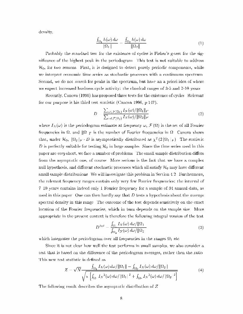
Probably the standard test for the existence of cycles is Fisher's g-test for the sig-

ni�cance of the highest peak in the periodogram. This test is not suitable to address

H0, for two reasons. First, it is designed to detect purely periodic components, while

we interpret economic time series as stochastic processes with a continuous spectrum.

Second, we do not search for peaks in the spectrum, but have an a priori idea of where

we expect increased business cycle activity: the classical ranges of 3-5 and 7-10 years.

Recently, Canova (1996) has proposed three tests for the existence of cycles. Relevant

for our purpose is his third test statistic (Canova 1996, p.147),

D =

P!2F(1)

IN (!)=k1kFP!2F(2)

IN (!)=k2kF (2)

where IN (!) is the periodogram estimate at frequency !, F () is the set of all Fourier

frequencies in , and kkF is the number of Fourier frequencies in . Canova shows

that, under H0, k2kF � D is asymptotically distributed as �2 (2k1kF ). The statistic

D is perfectly suitable for testing H0 in large samples. Since the time series used in this

paper are very short, we face a number of problems. The small sample distribution di�ers

from the asymptotic one, of course. More serious is the fact that we have a complex

null hypothesis, and di�erent stochastic processes which all satisfyH0 may have di�erent

small sample distributions. We will investigate this problem in Section 4.2. Furthermore,

the relevant frequency ranges contain only very few Fourier frequencies: the interval of

7{10 years contains indeed only 1 Fourier frequency for a sample of 34 annual data, as

used in this paper. One can then hardly say that D tests a hypothesis about the average

spectral density in this range. The outcome of the test depends sensitively on the exact

location of the Fourier frequencies, which in turn depends on the sample size. More

appropriate in the present context is therefore the following integral version of the test

DInt =

R1IN (!) d!=k1kR

2IN (!) d!=k2k (3)

which integrates the periodogram over all frequencies in the ranges 1 etc.

Since it is not clear how well the test performs in small samples, we also consider a

test that is based on the di�erence of the periodogram averages, rather then the ratio.

This new test statistic is de�ned as

Z =pN

R1IN (!) d!=k1k �

R2IN (!) d!=k2kr

�hR

1IN

2(!) d!=k1k2 +R2IN

2(!) d!=k2k2i (4)

The following result describes the asymptotic distribution of Z.

8

Proposition 1. Under H0, the statistic Z in (4) is asymptotically distributed as stan-

dard normal.

Proof. The asymptotic expectation ofRAIN d! is equal to

RAh(!) d! (Priestley 1981,

p.473), so that the numerator of Z has asymptotically zero expectation under the null

hypothesis. In addition, it is normally distributed: the integrated cumulative peri-

odogram is asymptotically distributed as a time-stretched Brownian motion (Priestley

1981, p.474). The asymptotic variance ofRAIN d! is equal to 2�

RAh2(!) d! (Priestley

1981, p.474). Since 12

RAIN

2 d! is a consistent estimator forRAh2(!) d! (Priestley 1981,

p.477), the claim follows.

The following section will compare the small sample properties of the di�erent test

statistics.

4.2 Small sample properties

The international data series available for our purposes are very short and comprise only

34 annual observations. For such short time series, the distribution of the test statistics

D, DInt and Z is far from their asymptotic distribution. More importantly, the small

sample distribution is not the same for all processes satisfying our composite hypothesis

H0. In a �rst step, we therefore examine how strongly the distribution varies under a

wide variety of processes which all satisfy the null hypothesis. Afterwards we investigate

the power of the tests to detect deviations from H0.

The null hypotheses appropriate to test the Classical Business Cycle Hypothesis as

de�ned at the end of the Introduction, are special cases of (1). In both cases, 2 =

R =�2�15 ;

2�10

�[ �2�7 ; 2�5 �[ �2�3 ; 2�2 �. For the test on the long cycle, 1 = L =�2�10 ;

2�7

�,

while for the short cycle, 1 = S =�2�5 ;

2�3

�. The corresponding test statistics are

denoted by Dlc, Dsc etc.

Distribution under H0

We use Monte-Carlo experiments to study the small sample distribution of the test

statistics for a wide variety of processes that satisfy H0. We consider a white noise

process as well as 24 di�erent ARMA processes, where the order of the AR parts is

between 1 and 5, and the order of the MA parts between 3 and 16. The processes 1{12

satisfy H0 for the long cycle, processes 13{24 for the short cycle. The processes have

zero, one or two internal maxima. The spectral densities of all 24 processes are shown

in Figures 4 and Figures 5 of Appendix A.

We take the white noise process as the reference case, from which we obtain the crit-

ical values. Table 1 presents critical values for di�erent percentiles, as well as expected

9

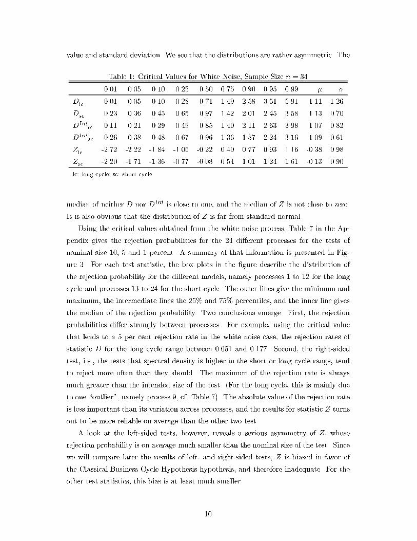
value and standard deviation. We see that the distributions are rather asymmetric. The

Table 1: Critical Values for White Noise, Sample Size n = 34

0.01 0.05 0.10 0.25 0.50 0.75 0.90 0.95 0.99 � �

Dlc 0.01 0.05 0.10 0.28 0.71 1.49 2.58 3.51 5.91 1.11 1.26

Dsc 0.23 0.36 0.45 0.65 0.97 1.42 2.01 2.45 3.58 1.13 0.70

DIntlc 0.11 0.21 0.29 0.49 0.85 1.40 2.11 2.63 3.98 1.07 0.82

DIntsc 0.26 0.38 0.48 0.67 0.96 1.36 1.87 2.24 3.16 1.09 0.61

Zlc -2.72 -2.22 -1.84 -1.06 -0.22 0.40 0.77 0.93 1.16 -0.38 0.98

Zsc -2.20 -1.71 -1.36 -0.77 -0.08 0.54 1.01 1.24 1.61 -0.13 0.90

lc: long cycle; sc: short cycle

median of neither D nor DInt is close to one, and the median of Z is not close to zero.

It is also obvious that the distribution of Z is far from standard normal.

Using the critical values obtained from the white noise process, Table 7 in the Ap-

pendix gives the rejection probabilities for the 24 di�erent processes for the tests of

nominal size 10, 5 and 1 percent. A summary of that information is presented in Fig-

ure 3. For each test statistic, the box plots in the �gure describe the distribution of

the rejection probability for the di�erent models, namely processes 1 to 12 for the long

cycle and processes 13 to 24 for the short cycle. The outer lines give the minimum and

maximum, the intermediate lines the 25% and 75% percentiles, and the inner line gives

the median of the rejection probability. Two conclusions emerge. First, the rejection

probabilities di�er strongly between processes. For example, using the critical value

that leads to a 5 per cent rejection rate in the white noise case, the rejection rates of

statistic D for the long cycle range between 0.051 and 0.177. Second, the right-sided

test, i.e., the tests that spectral density is higher in the short or long cycle range, tend

to reject more often than they should. The maximum of the rejection rate is always

much greater than the intended size of the test. (For the long cycle, this is mainly due

to one \outlier", namely process 9, cf. Table 7). The absolute value of the rejection rate

is less important than its variation across processes, and the results for statistic Z turns

out to be more reliable on average than the other two test.

A look at the left-sided tests, however, reveals a serious asymmetry of Z, whose

rejection probability is on average much smaller than the nominal size of the test. Since

we will compare later the results of left- and right-sided tests, Z is biased in favor of

the Classical Business Cycle Hypothesis hypothesis, and therefore inadequate. For the

other test statistics, this bias is at least much smaller.

10

0

0.1

0.2

0.3

0.4

0.5

0

0.1

0.2

0.3

0.4

0.5

0.10 0.05 0.01 0.10 0.05 0.01

DDIntZ DDIntZ DDIntZ DDIntZ DDIntZ DDIntZ

DDIntZ DDIntZ DDIntZ DDIntZ DDIntZ DDIntZ

Size of test

rejection probabilities

short cycle

long cycle

left-sided test right-sided test

left-sided test right-sided test

Figure 3: Rejection probabilities for 24 ARMA processes

11

Power

Next we investigate the power of our test statistic. We consider AR(2) processes that

have a peak in one of the business cycle frequency ranges. Table 2 presents the simulation

results. The columns \Period" and \�" denote the period (the inverse frequency) and

the modulus of the roots of the characteristic polynomial of the process. The limit case

of modulus � = 0 is equivalent to white noise, the higher �, the greater is the deviation

from the null hypothesis. The deviation from H0 is also measured by Qlong and Qshort,

which give the ratio of the spectral density in the long cycle region or short cycle region

to the spectral density in the other relevant regions. These statistics are the theoretical

counterparts toDInt. As to be expected, increasing the modulus � increases the rejection

probability of all three tests of the frequency range in which the process has its cycle.

The rejection probability for the other frequency range is declining strongly in �, since a

spectral peak in one range leads to increased spectral density in the neighboring ranges

which belong to R. The power of DInt to detect this kind of violation of the null

Table 2: Rejection Probabilities, AR(2)-Models,n = 34, Power: 0.05

Period � Qlong Qshort Dlc DIntlc Zlc Dsc DInt

sc Zsc

8.000 0.135 1.434 1.049 0.036 0.039 0.035 0.014 0.013 0.011

8.000 0.368 2.267 0.929 0.124 0.148 0.124 0.020 0.011 0.007

8.000 0.741 4.589 0.377 0.302 0.449 0.355 0.005 0.001 0.000

8.000 0.905 13.275 0.192 0.550 0.800 0.685 0.001 0.000 0.000

8.000 0.990 168.813 0.157 0.910 0.987 0.965 0.000 0.000 0.000

4.000 0.135 1.006 1.040 0.012 0.012 0.011 0.013 0.013 0.013

4.000 0.368 1.024 1.347 0.015 0.013 0.011 0.037 0.039 0.035

4.000 0.741 0.916 4.041 0.012 0.009 0.007 0.525 0.561 0.469

4.000 0.905 0.839 13.851 0.008 0.005 0.003 0.934 0.950 0.875

4.000 0.990 0.825 155.533 0.003 0.001 0.001 0.997 0.999 0.968

7.140 0.819 4.881 0.342 0.288 0.497 0.393 0.005 0.001 0.000

7.140 0.905 6.707 0.189 0.298 0.623 0.455 0.002 0.000 0.000

6.830 0.905 4.070 0.180 0.188 0.465 0.313 0.002 0.000 0.000

6.830 0.819 3.976 0.370 0.234 0.416 0.319 0.009 0.002 0.001

hypothesis is somewhat higher than that of Z, and considerably higher than that of

D, in particular if the cycle is close to the boundary of the long cycle range. Statistic

DInt therefore appears to be the best compromise between power and reliability in the

sense of the last subsection, and we have decided to use DInt in the rest of the paper.

12

The di�erences between the three tests are not big, however, and the empirical results

presented in the next section are not essentially altered if we use any of the other two

test statistics.

5 Empirical business cycles in 15 OECD countries

5.1 Data

The data series contain annual observations from 1960 to 1993 of real GDP, gross �xed

capital formation (GFCF) and inventory investment (II) of 15 OECD countries for which

the data are available since 1960. We work with annual rather than quarterly data since

the latter are not available since 1960 for most of the countries. The switch to higher-

frequency observations would tend to increase the e�ciency of the estimation, but this

e�ect is probably more than outweighed by the reduction in the sample period, if one is

concerned with identifying cycles of a �xed frequency range (here 3{5 and 7{10 years).

This is because the number of Fourier frequencies in a given frequency range is not

increased by a switch to higher frequency data.

5.2 Results

Table 3 presents a summary of the empirical results for the 15 OECD countries and for

the 5 di�erent detrending methods. For example, an entry n=m in the column II of the

long cycle means that the statistic DIntlc is signi�cantly greater than 1 in the inventory

investment series of n countries, and signi�cantly smaller than 1 in m countries. The

signi�cance level is 5% (one-sided), but one should remember that the critical value

was obtained from the white noise series (cf. Table 1), which probably underestimates

the size of the test. Despite di�erences between detrending techniques, a very clear

pattern emerges. First, the average spectral density of �xed investment in the long

cycle range is often signi�cantly higher than in the non-business cycle ranges, it is never

signi�cantly lower. A similar conclusion holds for GDP, but the result here seems more

sensitive to detrending. Second, the average spectral density of inventory investment in

the short cycle range is often signi�cantly higher than in the non-business cycle ranges,

and it is never signi�cantly lower. For �xed investment and GDP, there are practically

no signi�cant results for the short cycle. This is exactly the pattern predicted by the

classical view, with the exception that the inventory cycle is not found in GDP data. The

results show that detrending doesmatter. In particular, the di�erence �lter leads to fewer

signi�cant results. But it is also clear that detrending is not responsible for the main

conclusion. The qualitative results are the same for all the detrending techniques used,

13

Table 3: Number of Signi�cant Results

long cycle short cycle

II GFCF GDP II GFCF GDP

HP 0/0 11/0 12/0 3/0 1/3 0/1

Di� 0/6 5/0 2/0 3/0 1/0 0/0

Di�+LinTr 0/6 5/0 1/0 3/0 1/0 0/0

Baxter-King 0/2 8/0 9/0 5/0 1/0 0/0

Mod. Baxter-King 0/3 8/0 6/0 4/0 2/0 0/0n=m: statistic DIntis signi�cantly > 1 in n countries, signi�cantly

< 1 in m countries (signi�cance level: 5 per cent, one-sided). Results

for (modi�ed) Baxter-King �lter use critical values obtained for the

truncated sample size (n=28).

and the systematic di�erences in the results for �xed investment, inventory investment

and GDP cannot be caused by the detrending �lter, since the same �lter has been

applied to all series.

The detailed results for the modi�ed Baxter-King �lter are presented in Table 4

(detailed results for the other �lters are presented in Tables 8{11 in the Appendix). Of

the nine signi�cant long cycles in GFCF, six are signi�cant at the 1% level, while the

short cycle in II is signi�cant at the 1% level only in Germany. Italy, Sweden and the US

are the only countries that do not signi�cantly ful�ll the classical hypothesis for either

cycle.

14

Table 4: Modi�ed Baxter-King Filter, DInt

long cycle short cycle

II GFCF GDP II GFCF GDP

AUS 0:16�� 5:55??? 2:51? 0:92 4:79??? 1:37

AUT 0:82 3:85?? 2:58? 2:32? 1:26 1:66

BEL 1:07 0:94 3:51?? 2:24? 0:85 1:44

CAN 0:53 5:01??? 1:79 1:32 0:99 1:07

DNK 0:66 3:30?? 2:71? 3:05?? 0:93 2:08?

FRA 0:64 13:44??? 6:54??? 2:09? 1:21 1:67

WGR 1:34 6:29??? 3:76?? 4:29??? 0:89 2:09?

ITA 0:35 1:65 2:08 1:37 0:73 0:93

JPN 0:34 5:58??? 3:31?? 1:53 0:86 1:01

NDL 0:39 2:26? 1:79 1:96? 0:66 1:50

NZL 1:03 6:05??? 2:95?? 2:10? 0:88 1:35

NOR 0:50 0:84 2:75? 1:32 1:27 0:52

SWE 0:09�� 1:56 0:96 1:61 2:14? 1:39

UK 0:31 0:73 2:07 2:62?? 1:03 0:99

USA 0:22� 1:59 0:92 0:96 0:58 0:58

?=??=???: statistic is signi�cantly > 1 (10/5/1 per cent signi�cance level)

�=��=���: statistic is signi�cantly < 1 (10/5/1 per cent signi�cance level)

The absolute values of the test statistics in Table 4 show that the variations in

average spectral density are not only statistically signi�cant, but of substantial size.

For example, in France the average spectral density of GFCF in the long cycle range is

12.78 times as high than in the non-cycle ranges. The importance of the uctuations in

the classical frequency ranges can perhaps be illustrated even better by the fraction of

the spectral mass (variance) in these ranges, compared to the total spectral mass (Cf.

Table 13 of the appendix). While the length of the frequency range of the long cycle is

only 9.89% of the total range from 1=15 to 1=2, it contains a much higher fraction of the

total spectral mass. For the 9 countries with signi�cant long cycle in GFCF, this fraction

ranges from 21.0% in the case of Australia to 57.9% in the case of France. The fraction

is higher than one third also in Canada, West Germany, Japan and New Zealand. The

length of the short cycle range is 30.77%, but the fraction of the spectral mass of II it

contains ranges from 48.2% in New Zealand to 64.5% in Germany (considering only the

countries with signi�cant short cycle).

To provide more detailed information on the characteristics of the spectra of GFCF

15

and II, Table 5 lists the average spectral densities for all 5 frequency ranges.

Table 5: Average Spectral Densities, MBK Filter

II GFCF

[ 115 ;110 ] [ 110 ;

17 ] [17 ;

15 ] [15 ;

13 ] [13 ;

12 ] [ 115 ;

110 ] [ 110 ;

17 ] [17 ;

15 ] [15 ;

13 ] [13 ;

12 ]

AUS 0.002 0.005 0.023 0.010 0.016 0.208 0.385 0.206 0.243 0.108

AUT 0.004 0.018 0.028 0.028 0.007 0.220 1.095 0.415 0.192 0.122

BEL 0.002 0.006 0.004 0.009 0.006 1.738 0.276 0.145 0.259 0.146

CAN 0.009 0.005 0.013 0.005 0.006 0.686 1.035 1.006 0.194 0.120

DNK 0.006 0.005 0.005 0.006 0.004 2.446 5.116 2.320 0.654 0.182

FRA 0.002 0.005 0.001 0.010 0.006 0.178 0.892 0.168 0.048 0.033

WGR 0.001 0.015 0.009 0.014 0.003 0.757 2.626 0.631 0.171 0.041

ITA 0.000 0.007 0.003 0.012 0.012 0.600 0.627 0.822 0.229 0.045

JPN 0.002 0.001 0.002 0.003 0.002 1.239 1.714 0.119 0.163 0.093

NDL 0.002 0.005 0.005 0.009 0.005 0.515 1.341 0.732 0.087 0.073

NZL 0.014 0.049 0.026 0.069 0.066 8.662 5.959 0.352 0.659 0.222

NOR 0.037 0.015 0.114 0.045 0.014 1.812 0.883 0.650 0.673 0.179

SWE 0.006 0.004 0.088 0.033 0.004 0.147 0.035 0.058 0.199 0.041

UK 0.002 0.003 0.015 0.012 0.004 0.306 0.296 0.490 0.125 0.072

USA 0.001 0.002 0.007 0.004 0.003 0.224 1.495 2.995 0.242 0.096

We have mentioned in Section 2 that our de�nition of cycle is weak in the sense that

it does not require the spectral density of the long or short cycle range to be higher

than that of both neighboring ranges. The table shows that this stronger condition is

actually ful�lled for 8 of the nine cases with a signi�cant long cycle in GFCF. The only

exception is New Zealand, where the bulk of the spectral mass is located in the range

of 10{15 years, and which is therefore not really a candidate for a classical long cycle.

For the short cycle in II, the exception is UK, where average spectral density is slightly

higher in the range 5{7 than 3{5 years, and in Austria it is about the same in both

ranges.

For the cases without signi�cant results, di�erent patterns emerge. For GFCF, we

see that in Belgium and Norway the mass is concentrated in the range 10{15 years,

while for Sweden it is highest in the range 3{5 years. In Italy, UK and the US, spectral

density is highest in the range 5{7 years. This, however, depends on the �lter used. In

Italy and the US, spectral density is highest in the range 7{10 years if the HP �lter is

applied (cf. Table 12 in the Appendix). If the data do not show a clear pattern, the

16

results are dominated by the detrending �lter.

Finally, it might be interesting to compare the empirical results with the results

obtained from simulating the most basic neoclassical business cycle model. Table 6

reports the results for the RBC model of Cooley and Prescott (1995). The �xed invest-

ment series was converted to 34 annual observations. The simulation uses the original

calibration of parameters, which is for the USA. We see that the model produces a time

series whose �rst di�erences have an approximately at spectrum. Applying di�erent

detrending �lters we then obtain results which correspond to the respective �lter gain

functions. As we know from Cogley and Nason (1995), the dynamics of output and its

aggregates in this model is not signi�cantly di�erent from the dynamics of the exogenous

technological shock. The model does not produce cycles as they are found in the data

of most countries, unless we postulate the existence of cycles in technological progress.

Table 6: Average Spectral Densities GFCF, RBC model

Trend [ 115 ;110 ] [ 110 ;

17 ] [17 ;

15 ] [15 ;

13 ] [13 ;

12 ]

First Di�erences 1.999 2.083 2.003 1.626 1.106

HP 4.83 3.464 1.948 0.832 0.335

BK 1.549 2.321 2.323 0.992 0.309

MBK 1.110 1.706 1.801 0.897 0.310

Note: Average of 1000 repetitions.

6 Conclusions

The aim of this paper was to demonstrate that the classical view of business cycles,

as we have interpreted it, has an important element of truth. Obviously, the classical

view is not correct in a very strict sense: not every country has signi�cant cyclical

structure in the same frequency range. One could not plausibly expect such a strong

proposition to hold. Too di�erent are the economic structures in the di�erent countries,

and the economic shocks they are subjected to. Nevertheless, the data support the

predictions of the classical writers: �xed investment tends to have more spectral mass

in the frequency range of 7{10 years, inventory behavior in the range of 3{5 years.

Looking at each country separately, these regularities are often not signi�cant in the

statistical sense, which is not too surprising given the shortness of the available time

series. The signi�cance comes mainly from the similarity of results across countries.

We �nd it remarkable that international data starting in 1960 support a hypothesis

that has been established until the 1950s, using data from the 19th and the �rst half

17

of the 20th century. We think that the existence of these cycles is a stylized fact that

current business cycle theory should pay more attention to. The dynamics of �xed

investment is not explained by the most standard RBC model, since investment series

contain more dynamics than neoclassical theories predict (Sensenbrenner 1991). Wen

(1998) is a recent attempt to explain the cycle in �xed investment by a theory based on

investment complementarities.

References

Aftalion, A.: 1909, La realit�e des superproductions g�en�erales, Revue d'�economie politique

23(3), 201{29.

Baxter, M. and King, R. G.: 1995, Measuring business cycles: Approximate band-pass

�lters for economic time series, NBER Working Paper No. 5022.

Burns, A. F. and Mitchell, W. C.: 1946, Measuring Business Cycles, National Bureau

of Economic Research, New York.

Burnside, C.: 1998, Detrending and business cycle facts: A comment, Journal of Mon-

etary Economics 41(3), 513{532.

Canova, F.: 1996, Three tests for the existence of cycles in time series, Ricerche Eco-

nomiche 50, 135{62.

Canova, F.: 1998a, Detrending and business cycle facts, Journal of Monetary Economics

41(3), 475{512.

Canova, F.: 1998b, Detrending and business cycle facts: A user's guide, Journal of

Monetary Economics 41(3), 533{540.

Cogley, T. and Nason, J. M.: 1995, Output dynamics in real-business-cycle models,

American Economic Review 85(3), 492{511.

Cooley, T. F. and Prescott, E. C.: 1995, Economic growth and business cycles, in T. F.

Cooley (ed.), Frontiers of Business Cycle Research, Princeton University Press,

Princeton.

Cooley, T. F. (ed.): 1995, Frontiers of Business Cycle Research, Princeton University

Press, Princeton.

Davis, H. T.: 1941, The Analysis of Economic Time Series, Principia Press, San Anto-

nio, Texas.

18

Gale, D.: 1996, Delay and cycles, Review of Economic Studies 63(2), 169{98.

Granger, C.: 1966, The typical spectral shape of an economic variable, Econometrica

34, 150{161.

Hillinger, C. and Sebold-Bender, M.: 1992, The stylized facts of macroeconomic uc-

tuations, in C. Hillinger (ed.), Cyclical Growth in Market and Planned Economies,

Clarendon Press, Oxford.

Juglar, C.: 1862, Crises commerciales et leur retour p�eriodique en France, en Angleterre

et aux Etats-Unis, Guilaumin, Paris.

Kitchin, J.: 1923, Cycles and trends in economic factors, Review of Economics and

Statistics 5(1), 10{17.

Kuznetz, S.: 1926, Cyclical Fluctuations: Retail and Wholesale Trade, United States

,1919-1925, Adelphi, New York.

Matthews, R.: 1959, The Business Cycle, The University of Chicago Press.

Priestley, M.: 1981, Spectral Analysis and Time Series, Vol.1: Univariate series, Aca-

demic Press, New York.

Sargent, T. J.: 1987, Macroeconomic Theory, second edn, Academic Press, San Diego.

Schumpeter, J. A.: 1939, Business Cycles, McGraw-Hill, New York.

Sensenbrenner, G.: 1991, Aggregate investment, the stock market, and the q model:

Robust results for six oecd countries, European Economic Review 35(4), 769{825.

Watson, M. M.: 1993, Measures of �t for calibrated models, Journal of Political Economy

101(6), 1011{41.

Wen, Y.: 1998, Investment cycles, Journal of Economic Dynamics and Control 22, 1139{

65.

Woitek, U.: 1996, The G7-countries: A multivariate description of business cycle stylized

facts, in G. G. William Barnett and C. Hillinger (eds), Dynamic Disequilibrium

Modelling: Theory and Applications, Cambridge University Press, Cambridge.

Woitek, U.: 1998, A note on the Baxter-King �lter, University of Glasgow, Discussion

Papers in Economics No. 9813.

19

A Appendix: Detailed Tables and Figures

Table 7: Rejection probabilities for 24 di�erent stochastic processes

Prob. of greater value Prob. of greater valueProcess 0.95 0.10 0.05 0.01 Process 0.95 0.10 0.05 0.01

Statistic D1 0.950 0.108 0.056 0.013 13 0.932 0.121 0.069 0.0182 0.948 0.129 0.073 0.019 14 0.924 0.228 0.162 0.0723 0.956 0.161 0.095 0.036 15 0.923 0.236 0.168 0.0784 0.946 0.076 0.037 0.008 16 0.927 0.139 0.084 0.0255 0.942 0.081 0.036 0.007 17 0.918 0.248 0.180 0.0896 0.949 0.145 0.090 0.029 18 0.927 0.239 0.168 0.0757 0.945 0.088 0.041 0.010 19 0.939 0.102 0.052 0.0138 0.959 0.159 0.090 0.028 20 0.903 0.239 0.172 0.0839 0.959 0.204 0.134 0.059 21 0.937 0.372 0.296 0.16810 0.941 0.062 0.029 0.005 22 0.934 0.113 0.067 0.01711 0.948 0.111 0.059 0.014 23 0.909 0.250 0.188 0.08812 0.945 0.091 0.044 0.009 24 0.940 0.204 0.135 0.055

Statistic DInt

1 0.945 0.104 0.051 0.013 13 0.937 0.130 0.075 0.0192 0.947 0.123 0.069 0.017 14 0.925 0.187 0.122 0.0463 0.954 0.166 0.101 0.034 15 0.930 0.189 0.128 0.0504 0.935 0.099 0.051 0.012 16 0.935 0.146 0.087 0.0265 0.941 0.112 0.062 0.013 17 0.926 0.200 0.134 0.0596 0.968 0.226 0.149 0.057 18 0.926 0.186 0.120 0.0487 0.937 0.105 0.060 0.014 19 0.948 0.108 0.057 0.0138 0.954 0.126 0.071 0.019 20 0.904 0.186 0.127 0.0529 0.959 0.249 0.177 0.078 21 0.930 0.254 0.183 0.08410 0.909 0.101 0.053 0.012 22 0.939 0.127 0.071 0.01811 0.946 0.107 0.057 0.013 23 0.911 0.196 0.133 0.05612 0.945 0.105 0.056 0.013 24 0.939 0.153 0.092 0.030

Statistic Z1 0.953 0.102 0.049 0.012 13 0.964 0.117 0.064 0.0122 0.992 0.109 0.059 0.011 14 0.995 0.136 0.076 0.0163 0.999 0.144 0.079 0.020 15 0.996 0.138 0.076 0.0174 0.945 0.095 0.046 0.010 16 0.967 0.122 0.063 0.0145 0.965 0.097 0.048 0.006 17 0.996 0.133 0.070 0.0116 0.999 0.184 0.107 0.029 18 0.995 0.140 0.080 0.0207 0.953 0.097 0.050 0.011 19 0.956 0.107 0.058 0.0128 0.998 0.111 0.058 0.011 20 0.994 0.118 0.058 0.0079 1.000 0.215 0.138 0.050 21 0.999 0.150 0.074 0.01010 0.927 0.089 0.042 0.006 22 0.965 0.122 0.066 0.01511 0.961 0.103 0.054 0.012 23 0.994 0.119 0.058 0.00712 0.954 0.102 0.054 0.013 24 0.993 0.125 0.070 0.016

20

1)

15 10 7 5 3 2

2)

15 10 7 5 3 2

3)

15 10 7 5 3 2

4)

15 10 7 5 3 2

5)

15 10 7 5 3 2

6)

15 10 7 5 3 2

7)

15 10 7 5 3 2

8)

15 10 7 5 3 2

9)

15 10 7 5 3 2

10)

15 10 7 5 3 2

11)

15 10 7 5 3 2

12)

15 10 7 5 3 2

Figure 4: Spectral densities of test processes 1{12

21

13)

15 10 7 5 3 2

14)

15 10 7 5 3 2

15)

15 10 7 5 3 2

16)

15 10 7 5 3 2

17)

15 10 7 5 3 2

18)

15 10 7 5 3 2

19)

15 10 7 5 3 2

20)

15 10 7 5 3 2

21)

15 10 7 5 3 2

22)

15 10 7 5 3 2

23)

15 10 7 5 3 2

24)

15 10 7 5 3 2

Figure 5: Spectral densities of test processes 13{24

22

Table 8: Hodrick-Prescott Filter, DInt

long cycle short cycleII GFCF GDP II GFCF GDP

AUS 0:40 7:57??? 3:91?? 0:85 2:54?? 1:17AUT 1:83 4:40??? 3:38?? 2:49?? 0:77 0:91BEL 1:96 1:15 5:60??? 2:05? 0:24��� 0:73CAN 1:29 6:06??? 2:97?? 0:92 0:43� 0:40�

DNK 0:51 3:64?? 3:31?? 1:17 0:48 1:18FRA 2:01 11:66??? 7:99??? 1:35 0:48 0:64WGR 2:23? 6:90??? 3:62?? 2:72?? 0:55 0:98ITA 0:97 3:66?? 4:39??? 1:33 0:44� 0:56JPN 1:60 7:35??? 4:18??? 1:59 0:36�� 0:44�

NDL 0:44 3:43?? 1:14 1:60 0:42� 0:48NZL 2:00 3:28?? 3:20?? 1:79 0:35�� 0:52NOR 1:16 1:22 4:41??? 1:12 0:59 0:35��

SWE 0:24� 2:02 1:79 1:40 0:53 0:53UK 1:18 2:15? 3:36?? 2:82?? 0:43� 0:41�

USA 0:69 3:47?? 2:32? 0:92 0:58 0:39�

?=??=???: statistic is signi�cantly > 1 (10/5/1 per cent signi�cance level)�=��=���: statistic is signi�cantly < 1 (10/5/1 per cent signi�cance level)

Table 9: Di�erence Filter, DInt

long cycle short cycleII GFCF GDP II GFCF GDP

AUS 0:15�� 3:14?? 1:74 0:51 2:80?? 1:04AUT 0:63 1:99 2:18? 2:54?? 1:01 1:30BEL 0:38 0:53 2:50? 1:34 0:60 0:83CAN 0:46 3:74?? 1:57 0:91 0:75 0:95DNK 0:19�� 1:94 1:83 0:92 1:16 1:83FRA 0:37 6:50??? 4:26??? 1:20 0:71 0:94WGR 0:47 4:54??? 2:91?? 2:66?? 1:03 1:58ITA 0:15�� 2:40? 1:39 1:00 0:70 0:81JPN 0:37 3:58?? 2:37? 1:61 0:53 0:62NDL 0:18�� 1:19 1:00 1:46 0:92 0:44�

NZL 0:37 2:53? 1:65 1:19 0:93 0:92NOR 0:46 0:46 1:97 1:30 1:12 0:59SWE 0:13�� 1:69 1:48 1:41 0:71 0:69UK 0:53 0:73 1:88 2:73?? 1:14 0:94USA 0:15�� 2:30? 1:12 0:85 0:94 0:80?=??=???: statistic is signi�cantly > 1 (10/5/1 per cent signi�cance level)�=��=���: statistic is signi�cantly < 1 (10/5/1 per cent signi�cance level)

23

Table 10: Di�erence Filter + Linear Trend, DInt

long cycle short cycleII GFCF GDP II GFCF GDP

AUS 0:15�� 2:96?? 1:36 0:50 3:05?? 1:16AUT 0:61 1:53 1:14 2:53?? 0:90 1:44BEL 0:36 0:55 1:69 1:35 0:61 0:98CAN 0:46 4:11??? 1:75 0:91 0:75 1:01DNK 0:20�� 2:06 1:37 0:94 1:22 1:90?

FRA 0:31 6:76??? 3:66?? 1:22 0:80 1:24WGR 0:44 3:99??? 1:91 2:66?? 0:97 1:66ITA 0:14�� 2:43? 1:91 1:00 0:73 1:00JPN 0:34 3:75?? 2:17? 1:59 0:63 0:93NDL 0:17�� 1:31 0:38 1:48 0:97 0:48NZL 0:37 2:33? 1:34 1:19 0:94 0:93NOR 0:44 0:58 2:32? 1:31 1:08 0:64SWE 0:12�� 1:71 0:88 1:42 0:80 0:99UK 0:53 0:92 2:12? 2:69?? 1:24 1:06USA 0:16�� 2:14? 1:18 0:85 0:96 0:82?=??=???: statistic is signi�cantly > 1 (10/5/1 per cent signi�cance level)�=��=���: statistic is signi�cantly < 1 (10/5/1 per cent signi�cance level)

Table 11: Baxter-King Filter, DInt

long cycle short cycleII GFCF GDP II GFCF GDP

AUS 0:20� 6:75??? 3:07?? 0:99 4:78??? 1:45AUT 0:96 4:50?? 3:10?? 2:10? 1:23 1:45BEL 1:42 1:04 4:20?? 2:42?? 0:79 1:35CAN 0:63 5:27??? 1:96 1:32 0:89 0:94DNK 0:82 3:63?? 3:11?? 3:09?? 0:76 1:81FRA 0:86 14:65??? 7:24??? 2:08? 1:07 1:47WGR 1:64 6:62??? 4:07?? 4:11??? 0:76 1:82ITA 0:46 1:75 2:32? 1:30 0:64 0:78JPN 0:45 6:32??? 3:75?? 1:40 0:78 0:88NDL 0:47 2:51? 2:02 1:91 0:53 1:40NZL 1:40 6:34??? 3:42?? 2:31? 0:75 1:24NOR 0:56 0:95 2:94?? 1:26 1:15 0:46SWE 0:10�� 1:66 1:08 1:57 1:94 1:37UK 0:36 0:81 2:25? 2:62?? 0:96 0:91USA 0:28 1:72 1:01 0:91 0:51 0:50?=??=???: statistic is signi�cantly > 1 (10/5/1 per cent signi�cance level)�=��=���: statistic is signi�cantly < 1 (10/5/1 per cent signi�cance level)

24

Table 12: Average Spectral Densities, HP Filter

II GFCF[ 115

;

1

10] [ 1

10;

1

7] [ 1

7;

1

5] [ 1

5;

1

3] [ 1

3;

1

2] [ 1

15;

1

10] [ 1

10;

1

7] [ 1

7;

1

5] [ 1

5;

1

3] [ 1

3;

1

2]

AUS 0.005 0.006 0.017 0.013 0.018 0.282 1.110 0.304 0.372 0.066AUT 0.010 0.019 0.024 0.026 0.005 0.619 0.969 0.344 0.169 0.098BEL 0.001 0.007 0.002 0.007 0.004 4.663 0.941 0.431 0.200 0.185CAN 0.017 0.008 0.006 0.006 0.004 1.724 2.436 0.588 0.172 0.074DNK 0.005 0.003 0.007 0.007 0.006 4.595 3.893 1.409 0.514 0.249FRA 0.009 0.011 0.003 0.007 0.005 0.590 1.677 0.144 0.070 0.054WGR 0.005 0.009 0.007 0.011 0.003 0.714 2.382 0.953 0.192 0.063ITA 0.003 0.006 0.004 0.008 0.008 0.662 1.871 1.637 0.223 0.094JPN 0.005 0.004 0.002 0.004 0.002 1.365 2.424 0.388 0.120 0.103NDL 0.003 0.003 0.013 0.010 0.004 1.150 1.097 0.541 0.134 0.079NZL 0.012 0.063 0.017 0.056 0.040 11.472 5.985 0.709 0.637 0.280NOR 0.039 0.036 0.088 0.035 0.010 2.828 0.795 0.819 0.383 0.158SWE 0.009 0.004 0.064 0.025 0.004 2.692 1.410 1.039 0.374 0.183UK 0.006 0.005 0.011 0.013 0.002 2.242 1.116 0.807 0.221 0.076USA 0.001 0.002 0.005 0.002 0.002 0.610 1.701 1.665 0.283 0.062

Table 13: spectral mass in frequency ranges, as fraction of total spectral mass in range1/2{1/15, MBK Filter

II GFCF[ 115

;

1

10] [ 1

10;

1

7] [ 1

7;

1

5] [ 1

5;

1

3] [ 1

3;

1

2] [ 1

15;

1

10] [ 1

10;

1

7] [ 1

7;

1

5] [ 1

5;

1

3] [ 1

3;

1

2]

AUS 0.009 0.018 0.220 0.318 0.435 0.022 0.210 0.069 0.563 0.135AUT 0.011 0.058 0.208 0.514 0.209 0.025 0.279 0.232 0.285 0.179BEL 0.004 0.076 0.081 0.497 0.342 0.263 0.098 0.141 0.277 0.221CAN 0.061 0.049 0.200 0.387 0.302 0.132 0.356 0.205 0.218 0.089DNK 0.008 0.041 0.145 0.587 0.218 0.089 0.271 0.283 0.238 0.119FRA 0.034 0.048 0.032 0.494 0.391 0.095 0.579 0.082 0.162 0.081WGR 0.014 0.065 0.143 0.645 0.134 0.054 0.418 0.307 0.184 0.037ITA 0.007 0.033 0.053 0.401 0.507 0.066 0.167 0.500 0.228 0.039JPN 0.042 0.031 0.129 0.429 0.369 0.157 0.391 0.138 0.188 0.126NDL 0.004 0.031 0.206 0.488 0.270 0.109 0.219 0.313 0.198 0.160NZL 0.008 0.076 0.058 0.482 0.377 0.248 0.409 0.065 0.185 0.094NOR 0.016 0.047 0.403 0.387 0.147 0.120 0.078 0.276 0.366 0.160SWE 0.008 0.008 0.461 0.451 0.072 0.170 0.110 0.150 0.469 0.102UK 0.025 0.021 0.215 0.563 0.175 0.181 0.073 0.310 0.322 0.114USA 0.009 0.024 0.305 0.325 0.338 0.031 0.169 0.565 0.192 0.042

25