1

Chapter 1

Are There Atoms in Molecules? ATOMS AND THE MOLECULAR STRUCTURE HYPOTHESIS

Richard F. W. Bader

McMaster University

Hamilton, Ontario L8S 4MI, Canada....

Introduction No one questions the importance to chemistry of the concept of atoms or of functional

groupings of atoms. We recognize a group in a molecule in terms of a characteristic set of properties assigned to that group and in properties of the molecule in terms of these same group properties. This concept, together with the rest of the molecular structure hypothesis, that a molecule consists of atoms linked by a network of bonds to yield a recognizable structure, is the cornerstone of chemical thinking. Let's be clear in our thinking. We consider a given property of a molecule to be the sum of the corresponding property for each of its constituent atoms or groups. Properties are additive. Group properties are also characteristic, that is, they are transferable to some degree. In some cases they appear experimentally, to be completely transferable to yield what are known as group additivity schemes for properties such as molar volumes, heats of formation, polarizabilities and magnetic susceptibilities.

This being the case, and with quantum mechanics having been with us now for 70 years,

why was there no development of a theory of atoms in molecules long ago that predicted all of this and why, instead, is there still a prevailing opinion among some that while being unquestionably useful, the concepts of atoms and bonds are incapable of precise or unique

. L.A. Montero, L.A. Díaz and R. Bader (eds.), Introduction to Advanced Topics of Computational Chemistry, 1 - 28, 2003, © 2003 Editorial de la Universidad de La Habana, Havana.

2

definition? The reason, I think, is partly the result of failed attempts, failed because people were looking in the wrong place for their definitions -, looking in Hilbert space, or if not directly, their thinking was dominated by the pictures of atoms obtained from orbital models in that space. From this arose the idea that an atom must extend over all space, and atoms are therefore, overlapping. This view precludes their quantum definition, as we shall later illustrate. There is another, deeper reason atoms were not defined and that is because their definition requires a new version of quantum mechanics. It has taken the reformulation of physics, as afforded by the work of Feynman and Schwinger, to provide us with the necessary quantum mechanical framework that lets one both ask and answer the question: “Are there atoms in molecules?”.

I want to present a theory that states that atoms do exist in molecules, and that each atom

is a bounded piece of real space. I want to introduce this theory to you in the very same manner that it evolved, to emphasize its essential observational basis –its basis in experimental chemistry.

The Role of the Electron Density Everything we can know about a system is contained in the state function. We use the

state function to determine the measurable eigenvalues or expectation values of the observables. Among these are the electron density and the electron current density. Schrödinger himself, in his fourth paper in which he introduced these quantities and the equation of continuity relating them, expressed the hope that their study would aid in our understanding of the electrical and magnetic properties of matter. I read ‘electrical’ now as the ‘electronic’ properties of matter. Those who state that the study of the electron density is something less than quantum mechanics fail to understand that the whole point of quantum mechanics is to use the wave function it provides to calculate the measurable properties of the observables and not, as Schrödinger warned us against, to view the wave function as an end in itself. The study of the properties of the electron density leads to a quantum theory of atoms in molecules.

The electron density ρ(r) is obtained in the following way: The probability that any one

electron will be in some infinitesimal volume element dτ with either an α or a β spin is obtained by integrating ψ* ψ over the space coordinates of all electrons but one and summing over all spin coordinates, (dxi = dτi multiplied by α or β spin and there are N electrons):

Multiplication of this result by N gives the probability of finding any of the electrons in

dτ1, and division by dτ1, to obtain a density - a probability per unit volume - yields the electron density at the point defined by the position vector r, the quantity ρ(r)

The mode of integration used in eqn. (2) appears throughout the theory in the definition

of density distributions for any property and is abbreviated to the form shown in eqn. (3):

For a system in a given quantum state, ρ(r) describes the distribution of charge

throughout three-dimensional space, a quantity now measured with great accuracy in many

3

laboratories. (Because of the cusp condition on ψ and hence on ρ, positions of nuclei and their respective charges are also determined by the density and thus ρ(r) determines the total charge distribution of a system.)

A partitioning of space based on the topology of the electron density Through a collaboration with the Mulliken-Roothaan laboratory in the 1960’s my

laboratory had access to near Hartree-Fock quality wave functions for nearly 300 diatomic molecules, in both ground and excited states, and we used these to study the properties of the electron density. I consider these studies to be “theoretical” experiments in the study of ρ. In principle, what we found for these diatomic molecules could now be observed in the densities obtained experimentally for solids, but at that time the experimental techniques and methods had not been perfected to the degree needed to obtain reliable densities.

Fig. 1. Two views of a transferable methylene group in a normal hydrocarbon as defined by the intersection of the van der Waals density envelope (ρ(r) = 0.001 au) with the two bounding C | C zero flux surfaces. The trajectories of ∇ρ (r) that terminate at a bond critical point in the density and define a zero flux surface between a pair of carbon atoms are shown in d. Also shown, is the unique pair of trajectories that originate at the same point and define the bond path linking the two carbon nuclei. Fig. c shows the structure, the bond paths linking the carbon to two protons and the two critical points in the C | C interatomic surfaces.

Eventually we realized that the topology of ρ(r) provided a unique partitioning of the space of a molecule, or a crystal, into mononuclear regions that I shall refer to as atoms. Equally important, it soon became apparent that the resulting regions were transferable to varying extents

4

between molecules. Indeed, if one insisted that the pieces transferred had to exhaust the system, they had the property of maximizing any transferability that was present.

This atomic form imposed on the structure of matter is a consequence of the principal

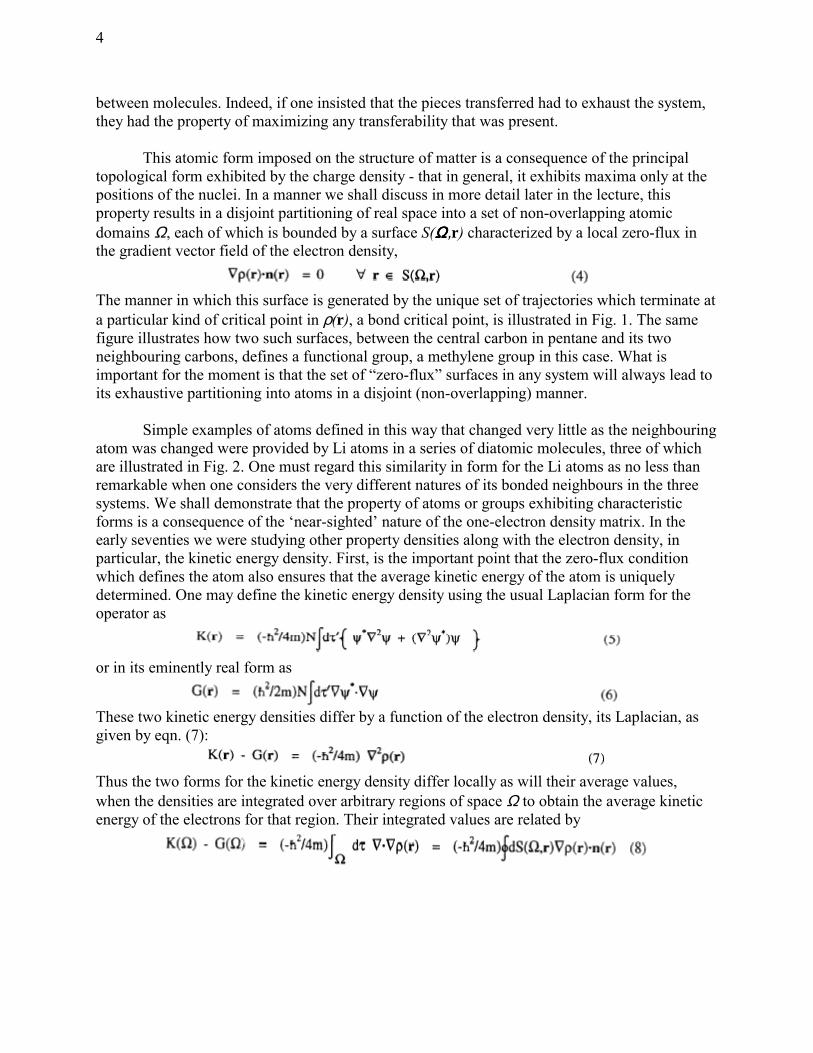
topological form exhibited by the charge density - that in general, it exhibits maxima only at the positions of the nuclei. In a manner we shall discuss in more detail later in the lecture, this property results in a disjoint partitioning of real space into a set of non-overlapping atomic domains Ω, each of which is bounded by a surface S(ΩΩΩΩ,r) characterized by a local zero-flux in the gradient vector field of the electron density,

The manner in which this surface is generated by the unique set of trajectories which terminate at a particular kind of critical point in ρ(r), a bond critical point, is illustrated in Fig. 1. The same figure illustrates how two such surfaces, between the central carbon in pentane and its two neighbouring carbons, defines a functional group, a methylene group in this case. What is important for the moment is that the set of “zero-flux” surfaces in any system will always lead to its exhaustive partitioning into atoms in a disjoint (non-overlapping) manner.

Simple examples of atoms defined in this way that changed very little as the neighbouring

atom was changed were provided by Li atoms in a series of diatomic molecules, three of which are illustrated in Fig. 2. One must regard this similarity in form for the Li atoms as no less than remarkable when one considers the very different natures of its bonded neighbours in the three systems. We shall demonstrate that the property of atoms or groups exhibiting characteristic forms is a consequence of the ‘near-sighted’ nature of the one-electron density matrix. In the early seventies we were studying other property densities along with the electron density, in particular, the kinetic energy density. First, is the important point that the zero-flux condition which defines the atom also ensures that the average kinetic energy of the atom is uniquely determined. One may define the kinetic energy density using the usual Laplacian form for the operator as

or in its eminently real form as

These two kinetic energy densities differ by a function of the electron density, its Laplacian, as given by eqn. (7):

Thus the two forms for the kinetic energy density differ locally as will their average values, when the densities are integrated over arbitrary regions of space Ω to obtain the average kinetic energy of the electrons for that region. Their integrated values are related by

5

Fig. 2. Contour plots of the ground state molecular charge distributions of LiF, LiO and LiH. The intersection of the interatomic surface with the plane shown in the diagram is indicated by the dashed line. Figures show the intersection of the zero-flux surfaces with the plane of the diagram. Note the great similarity in the distribution of density within the basin of the Li atom in all three molecules that is present in spite of the differing chemical nature of its bonded partner. At the Hartree-Fock level the populations of the Li atom differ by only 0.024 e between the least and most electronegative partners H and F while the spread in their energies is - 8 kcal/mole. The extent of transferability of the form of an atom in real space - that is, its charge distribution - is paralleled by a corresponding transferability in its energy. The contours increase in value 2x10n, 4x10n and 8x10n with n beginning at -3 and increasing in steps of unity.

6

Gauss’ theorem enables one to rewrite the volume integral of ρρ ∇⋅∇=∇ 2 as an integral of the flux in ρ∇ through the surface of Ω. Clearly this integral vanishes for an atom, as it does for the total system, because of the defining condition given in eqn. (4). Thus, as indicated in eqn. (9), the average electronic kinetic energy of an atom in a molecule, T(Ω), is well defined,

One notes that the average electronic kinetic energy defined in this manner is necessarily additive over any set of disjoint regions which exhaust the system

We observed in our study of the density distributions that the kinetic energy density K(r)

or G(r) over the basin of an atom up to its zero-flux surface, exhibited the same degree of transferability as did the electron density ρ(r), and thus the conservation in the form of ρ and consequently in its integrated electron population on transfer, was paralleled by a conservation in the electronic kinetic energy.

The paralleling transferability of ρ(r) and G(r) is illustrated in Figure 3 for the methylene

group adjacent to a methyl group in butane in one case and pentane in the other. This is the crucial observation that leads to the theory of atoms in molecules, as deduced from the following chain of reasoning. The virial theorem for a system with Coulombic forces states that the total energy equals minus the kinetic energy. In our case it states that the total electronic energy E equals the negative of the electronic kinetic energy T. If one could show that there is a virial theorem for an atom in a molecule - that is, for a region of space bounded by a zero-flux surface –then the above observation suggests that one could define the energy of atom in a molecule in terms of the atom’s electronic kinetic energy T(Ω)

and, since T(Ω) is additive, eqn. (10), this definition of the energy of an atom would necessarily be additive as well and the total energy of a molecule would be the sum of its atomic contributions,

Furthermore, one would know that when the form of the atom in real space remained

unchanged on transfer between systems, so did its contribution to the total energy. That is, by observation, the energy of an atom would be transferable to the same extent that the charge density was, and when an atom as it appeared in real space - that is, in terms of its distribution of charge - was transferable between systems, so was its energy. Surely if one could do this for the energy, all other properties would follow. Thus the topological atoms exhibit the very properties of additivity and transferability that are the operational essentials to the concept of atoms in molecules.

A spatial partitioning of the total energy is not a trivial problem, because it requires a partitioning of the potential energy contributions. We shall return to this in detail later, but briefly how does one spatially partition the energy of repulsion between the nuclei and between the electrons or partition the energy of attraction of each nucleus for all of the electrons? The answer is provided by the virial theorem which identifies the potential energy with the virial of the forces exerted on the electrons. A force, unlike the energy, is local. One can write down the

7

operator which determines the force exerted on one electron by all of the remaining particles in the system. Knowing the force exerted on an electron and hence on the electron density at a point in space, enables one to determine the potential energy of that element of density by taking the virial of the force. Integration of the resulting potential energy density or virial field over the basin of the atom yields V(Ω), its average potential energy. The energy E(Ω) of the atom can by the virial theorem, be alternatively expressed as the sum of T(Ω) and V(Ω). Figure 3 shows that this virial field is as transferable for the methylene group in butane and pentane as are the electron and kinetic energy densities. The total integrated numbers of electrons in the two groups differ by 0.00005 e and their energies by less than one kcal/mole.

Fig. 3. Contour maps for ρ(r) in (a), G(r) in (b) and VVVV(r) in (c) for the methylene group in butane (lhs) and pentane (rhs) obtained from MP2/6-311++G(2d,2p) calculations. The map for each field in butane is superimposable on the corresponding map in pentane, with charge conservation of 0.0005 e and with a change in energy of 0.88 kcal/mole. The contour values are the same as those used in Fig. 2 with the exception that the outermost contour in each map has the value 0.001 au.

8

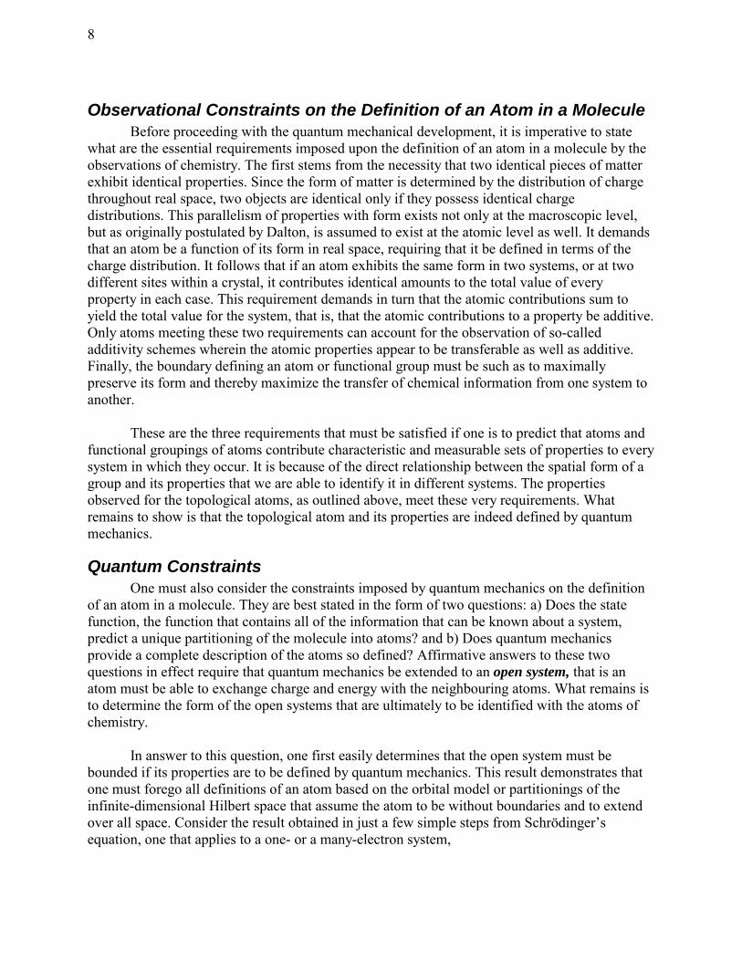
Observational Constraints on the Definition of an Atom in a Molecule Before proceeding with the quantum mechanical development, it is imperative to state

what are the essential requirements imposed upon the definition of an atom in a molecule by the observations of chemistry. The first stems from the necessity that two identical pieces of matter exhibit identical properties. Since the form of matter is determined by the distribution of charge throughout real space, two objects are identical only if they possess identical charge distributions. This parallelism of properties with form exists not only at the macroscopic level, but as originally postulated by Dalton, is assumed to exist at the atomic level as well. It demands that an atom be a function of its form in real space, requiring that it be defined in terms of the charge distribution. It follows that if an atom exhibits the same form in two systems, or at two different sites within a crystal, it contributes identical amounts to the total value of every property in each case. This requirement demands in turn that the atomic contributions sum to yield the total value for the system, that is, that the atomic contributions to a property be additive. Only atoms meeting these two requirements can account for the observation of so-called additivity schemes wherein the atomic properties appear to be transferable as well as additive. Finally, the boundary defining an atom or functional group must be such as to maximally preserve its form and thereby maximize the transfer of chemical information from one system to another.

These are the three requirements that must be satisfied if one is to predict that atoms and

functional groupings of atoms contribute characteristic and measurable sets of properties to every system in which they occur. It is because of the direct relationship between the spatial form of a group and its properties that we are able to identify it in different systems. The properties observed for the topological atoms, as outlined above, meet these very requirements. What remains to show is that the topological atom and its properties are indeed defined by quantum mechanics.

Quantum Constraints One must also consider the constraints imposed by quantum mechanics on the definition

of an atom in a molecule. They are best stated in the form of two questions: a) Does the state function, the function that contains all of the information that can be known about a system, predict a unique partitioning of the molecule into atoms? and b) Does quantum mechanics provide a complete description of the atoms so defined? Affirmative answers to these two questions in effect require that quantum mechanics be extended to an open system, that is an atom must be able to exchange charge and energy with the neighbouring atoms. What remains is to determine the form of the open systems that are ultimately to be identified with the atoms of chemistry.

In answer to this question, one first easily determines that the open system must be

bounded if its properties are to be defined by quantum mechanics. This result demonstrates that one must forego all definitions of an atom based on the orbital model or partitionings of the infinite-dimensional Hilbert space that assume the atom to be without boundaries and to extend over all space. Consider the result obtained in just a few simple steps from Schrödinger’s equation, one that applies to a one- or a many-electron system,

9

In eqn (13), ρG is the density of property G, represented by the operator (observable) G . Its time rate-of-change over some infinitesimal volume element dτ is given by the local expectation value of the commutator of G with H together with the final term which measures the net flow of the property G in or out of dτ in terms of the divergence of the current for property G, the term

)(rjG⋅∇ . We have here the two essential quantities needed to describe any property for any system, a density and its associated current. To determine the time rate of change of the average of the property G for some part of a system, one should integrate (13) over a region Ω to obtain

The final integral of the divergence of a vector is, by Gauss’ theorem, equivalent to an integral of the flux of the current jG(r) through the surface of the open system to yield

Gauss’ theorem brings each term in eqn (15), the equation of motion for the property G for an open system Ω, into correspondence with the a term in eqn (13) for the infinitesimal region dτ, with the final term in (15) determining the net outflow of the property G in terms of the flux in the property’s current density through its boundary surface. Thus the value of a property and its time rate of change are determined for bounded regions of space and an essential part of this description is provided the surface flux of the associated current density. The question remaining is whether any and all regions Ω have physical significance, or whether there is a special class of open systems, special in the sense that they and their properties would be defined and determined by the same physics that determines the properties of the total system of which they are a part.

The extension of quantum mechanics to an open system is indeed possible within the framework of the generalized action principle. The quantum mechanics of a proper open system can be simply outlined. It is based on the reformulation of physics provided by the work of Feynman and Schwinger, an approach that makes possible the asking and answering of questions not possible within the traditional Hamiltonian framework. It is important to appreciate that the alternative to the use of existing models and arbitrary definitions of chemical concepts is a theory of atoms in molecules that is rooted in physics.

QUANTUM MECHANICS OF AN ATOM IN A MOLECULE

From Dirac to Schwinger to Atoms in Molecules We begin our development of the quantum basis for the theory of atoms in molecules by

concentrating on the underlying ideas and we do so by beginning with Dirac, leaving the mathematical details to be filled in later. Dirac demonstrated the equivalence of Schrödinger’s wave mechanics and Heisenberg’s matrix mechanics, both of which are firmly rooted in classical Hamiltonian dynamics. Dirac accomplished this by introducing transformation theory into quantum mechanics, the underlying mathematical formalism of this new physics which consists of the general mathematical scheme of linear operators and state vectors with its associated probability interpretation. In doing so, he stressed how the theory of infinitesimal unitary

10

transformations in quantum mechanics parallels the infinitesimal canonical transformations of classical theory.

We give Dirac’s own words, taken from his book, on the importance of this analogy:

‘The variation with time of the Heisenberg dynamical variable may be looked upon as the continuous unfolding of an infinitesimal unitary transformation and similarly the classical dynamical variables at time t + δt are connected to their values at time t by an infinitesimal contact transformation and the whole motion may be looked upon as the continuous unfolding of a contact transformation. We have here the mathematical foundation of the analogy between the classical and quantum equations of motion, and can develop it to bring out the quantum analogues of all the main features of the classical theory of dynamics.’

In particular such arguments lead in 1933 to what was to be a paper of singular

importance. In it Dirac posed the question of what would correspond to the limiting classical expression for <q,t | q’,t’>, the quantum probability amplitude for the passage of a system with a set of coordinates denoted collectively by q at time t to another state with coordinates q’ at t’. In effect, Dirac was asking for what would correspond in quantum mechanics to the Lagrangian method of classical mechanics, a formulation he considered to be more fundamental than the one based on Hamiltonian theory. In the Lagrangian approach, the equation of motion that determines how a system proceeds from a state (q,t) to another (q’,t’) is obtained from the principle of least action. In this principle, the space-time trajectory connecting the ’ two classical states is the one that minimizes a quantity called the action, the time integral of the system’s Lagrangian.

The limiting classical expression for the quantum probability amplitude proposed by Dirac is:

where W is the solution to the Hamilton-Jacobi equation

and is the quantum analogue of the classical action function evaluated along the classical path connecting the two states and it equals it in the limit ħ approaching zero. To obtain this answer Dirac made use of the multiplicative law of transformation theory, which expresses the probability amplitude connecting two states as a product of contributions connecting intermediate states and, as a consequence, the associated action as a sum. The ideas in this paper formed the basis of the new formulations of quantum mechanics presented independently around 1950 by Feynman and by Schwinger.

In Feynman’s path integral formulation of quantum mechanics, the probability amplitude <q,t|q’,t’> is equated to a sum over all possible paths q(t) (an integral in the limit of a continuum of possible paths δq(t), in eqn (18)) connecting the two space- time points, rather than just the classically allowed one appearing in Dirac’s expression for the classical limit

where N is a normalizing factor. Thus each contributing path has the same modulus, but its phase is proportional to the classical action along the path, as given in Dirac’s expression. Feynman’s path integral expression can be shown to yield Schrödinger’s equation and the commutation relations.

11

Schwinger’s formulation of quantum mechanics is actually a differential form of

Feynman’s path integral expression. To see how Schwinger arrived at its form consider a system in just one spatial dimension, x. The quantum mechanical expression for the Lagrangian density L in this case is a function of ψ, ∂ψ/∂x and t (as opposed to q, dq/dt and t in the classical case) and the action integral is expressed as an integral over both space and time

and the integral thus defines a space-time volume. If the limits on x are at plus and minus infinity, one has the action for a isolated, total system. Note however, that the action is additive over the individual space-time areas obtained by subdividing x into line segments, Fig. 4.

Fig. 4. Diagramatic representation of the space-time area swept out by the action for a one-dimensional system with finite boundaries at x1 and x2. The variation of the action over the space-time area vanishes to yield the equation of motion, leaving only the contributions from the two space-like and two time-like surfaces.

Schwinger showed how one can obtain all the laws of physics by combining the action

principle with Dirac’s transformation theory. He does this by minimizing the Lagrangian in the space-time volume to obtain the equation of motion as is done in the classical principle of least action. However, unlike the procedure followed in that principle, the variations at the time end points are not equated to zero but are retained along with a variation of the time itself. These end point variations are then identified with the generators of infinitesimal unitary transformations of Dirac’s theory, since Schwinger realized that such transformations can be used to provide a differential characterization of a transformation function such as <q,t | q’,t’>. In extending the

12

principle to a subsystem of a total system, one also retains the variations both on and of the surface bounding the subsystem at each time. Thus Schwinger’s general formulation retains the variations at the time-like surfaces (the time evolution of the spatial boundary), as well as at the space-like surfaces (the system at the two time end points) that bound the desired piece of a system and identifies them with the generators of infinitesimal unitary transformations, Fig. 4. Schwinger calls this generalization of the action principle ‘the principle of stationary action’. For the total system with variations restricted to just the space-like surfaces at the two time end points, Schwinger postulates what is in effect a differential form of Feynman’s expression

The corresponding expression for ∂<q,t | q’,t’> obtained from Dirac’s transformation

theory in terms of infinitesimal generators Ĝ(t) acting at the two time end points is given by

A comparison of these two expressions leads to the principle of stationary action, eqn. (22)

that is, the variation in the action does not vanish, as it does in the principle of least action, but instead equals the difference in the values of the generators acting at the two time end points. This principle, like Feynman’s, yields Schrodinger’s equation and the commutation relations.

One can describe all physical changes, both temporal and spatial, in terms of the generators Ĝ(t). Thus one recovers all of physics in Schwinger’s principle of stationary action. In addition to yielding Schrödinger’s equation, it defines the observables of quantum mechanics, their equations of motion and their expectation values. These are precisely the properties which must be established and defined for a subsystem if one wishes to obtain a quantum prescription for an atom in a molecule.

Clearly, if one desires a definition of an atom based on physics, the atom must correspond to a piece of space-time and its boundaries must therefore, be defined in real space, the same conclusion arrived at earlier using the equation of motion for an observable eqn. (15), derived from Schrödinger’s equation. This is the reasoning underlying the basic tenet of the theory of atoms in molecules, which is that atoms be defined as pieces of real space.

The possibility of defining the action for a subsystem is a consequence of its fundamental additive nature, as discussed above. The variation of the action for a subsystem leads one down the same road traversed by Schwinger, but one does not arrive at the same destination (which he arrived at by considering only variations in the space-like surfaces) unless the subsystem satisfies a particular boundary condition on its time-like surfaces. This condition is imposed as a constraint on the variation of the action and it requires that the subsystem be bounded by a surface through which there is a zero flux in the gradient vector field of the electronic charge density.

The Quantum Description of an Atom in a Molecule The quantum action principle as presented by Schwinger, leads one in a natural and

objective manner to the generalization of quantum mechanics to a subsystem of a total system, that is to the definition of a proper open system. Rather than proceed with the demonstration of this in a formal way, we start here with Schrödinger’s development of quantum mechanics for a

13

stationary state as presented in his first paper in 1926 and show how Schwinger’s use of infinitesimal unitary transformations and their introduction via a generalized variation principle, enables one to extend Schrödinger’ s “wave mechanics” to an atom in a molecule. In doing so, one obtains the stationary state analogue of Schwinger’s principle of stationary action and the physics of an atom in a molecule.

Derivation of Subsystem Hypervirial Theorem Before starting the derivation of the principle of stationary action, let us introduce

ourselves to subsystem quantum mechanics and the manner in which it differs from the quantum mechanics for the total system. This difference is a result of operators no longer necessarily being Hermitian when averaged over a subsystem. This has the important result of introducing fluxes in property currents through the surface of the subsystem when deriving the Heisenberg equation of motion for an observable A, an equation which in the case of a stationary state considered here, is referred to by some as the hypervirial theorem. For a stationary state the theorem states that

a result that is easily proved simply by expanding the commutator and making use of the fact that Ĥ is Hermitian and that ψ and ψ* are eigenfunctions of the Hamiltonian operator.

In considering a subsystem one must, because of the loss of Hermiticity, consider the sum of <ψ,[Ĥ,Â]ψ>Ω and its complex conjugate and in addition, one can no longer assume that <ψ,ĤÂψ>Ω = <Ĥψ,Âψ>Ω. We shall detail the derivation for just the term <ψ,[Ĥ,Â]ψ>Ω. When the average of the commutator is taken over a subsystem, one adds and subtracts the term <Ĥψ,Âψ>Ω to the usual derivation of this theorem for a total, isolated system. This yields

Making use of Schrödinger’s equation that Ĥψ = Eψ for the last two terms on the RHS, and writing out the explicit form for a subsystem average denoted by < >Ω for the two remaining terms one has (assuming no derivatives are present in the potential energy operator V appearing in the Hamiltonian Ĥ)

Making use of Gauss’ theorem for transforming the volume integral of a divergence into a surface integral, one has

the surface term represents the flux in vector current density for the observable A(r) through the surface of the subsystem

Thus, for a subsystem, the commutator average of Ĥ and  is given by the flux in the property density of A through the surface of the subsystem,

14

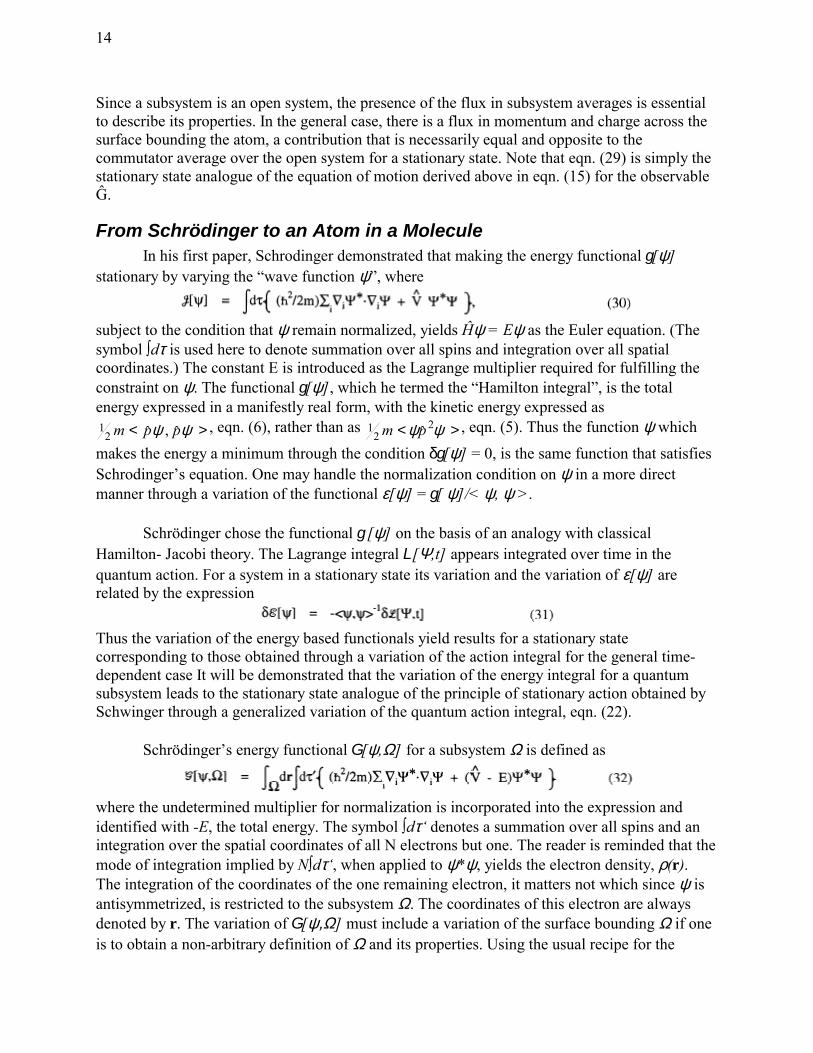
Since a subsystem is an open system, the presence of the flux in subsystem averages is essential to describe its properties. In the general case, there is a flux in momentum and charge across the surface bounding the atom, a contribution that is necessarily equal and opposite to the commutator average over the open system for a stationary state. Note that eqn. (29) is simply the stationary state analogue of the equation of motion derived above in eqn. (15) for the observable Ĝ.

From Schrödinger to an Atom in a Molecule In his first paper, Schrodinger demonstrated that making the energy functional g[ψ]

stationary by varying the “wave function ψ”, where

subject to the condition that ψ remain normalized, yields Ĥψ = Eψ as the Euler equation. (The symbol ∫dτ is used here to denote summation over all spins and integration over all spatial coordinates.) The constant E is introduced as the Lagrange multiplier required for fulfilling the constraint on ψ. The functional g[ψ], which he termed the “Hamilton integral”, is the total energy expressed in a manifestly real form, with the kinetic energy expressed as

>< ψψ ppm ˆ,ˆ21 , eqn. (6), rather than as >< ψψ 2

21 pm , eqn. (5). Thus the function ψ which

makes the energy a minimum through the condition δg[ψ] = 0, is the same function that satisfies Schrodinger’s equation. One may handle the normalization condition on ψ in a more direct manner through a variation of the functional ε[ψ] = g[ ψ]/< ψ, ψ >.

Schrödinger chose the functional g [ψ] on the basis of an analogy with classical Hamilton- Jacobi theory. The Lagrange integral L[Ψ,t] appears integrated over time in the quantum action. For a system in a stationary state its variation and the variation of ε[ψ] are related by the expression

Thus the variation of the energy based functionals yield results for a stationary state corresponding to those obtained through a variation of the action integral for the general time-dependent case It will be demonstrated that the variation of the energy integral for a quantum subsystem leads to the stationary state analogue of the principle of stationary action obtained by Schwinger through a generalized variation of the quantum action integral, eqn. (22).

Schrödinger’s energy functional G[ψ,Ω] for a subsystem Ω is defined as

where the undetermined multiplier for normalization is incorporated into the expression and identified with -E, the total energy. The symbol ∫dτ‘ denotes a summation over all spins and an integration over the spatial coordinates of all N electrons but one. The reader is reminded that the mode of integration implied by N∫dτ‘, when applied to ψ*ψ, yields the electron density, ρ(r). The integration of the coordinates of the one remaining electron, it matters not which since ψ is antisymmetrized, is restricted to the subsystem Ω. The coordinates of this electron are always denoted by r. The variation of G[ψ,Ω] must include a variation of the surface bounding Ω if one is to obtain a non-arbitrary definition of Ω and its properties. Using the usual recipe for the

15

variation of some functional, as described in my book or in Goldstien’s book on classical mechanics, one obtains the result given in eqn. (33). The integrand of the functional ϑ[ψ,Ω], denoted by f depends upon ψ and ψ∇ (and their complex conjugates, ψ* being treated independently of ψ in the variation) and thus the variation of G[ψ,Ω], including a variation of its surface, is of the form

where S(W,r) denotes the surface bounding the subsystem, a function of the coordinate r and δS denotes a variation of S through its dependence on ψ. Carrying out the steps indicated above one obtains

where the operator ∇ refers to the electron with coordinate r. The Hamiltonian appearing in eqn. (34) is

with V denoting the full many-particle potential energy operator. The first of the surface terms in eqn. (11) arises through the use of the integration by parts to rid the expression of variations in

ψ∇ , ie the final term in eqn. (36)

In this manner one obtains the form of the kinetic energy operator as it appears in Ĥ.

When Ω refers to the total system and G[ψ,Ω] reduces to G[ψ], a surface integral for the argument ( ) ( )δψψ iim rn⋅∇ *2/2

is obtained for each electron. In this case the surface S(ri) for every electronic coordinate ri occurs for ri = ∞ and the surface terms are made to vanish either by demanding that δψ = 0 when any ri = ∞, or by imposing the so-called natural boundary condition, that

One requires G[ψ] to be stationary with respect to arbitrary variations in ψ and in this case eqn. (34) reduces to

The condition that δG[ψ] be stationary for all arbitrary δψ or δψ* (which are considered to be independent variations), demands satisfaction of the corresponding Euler equations which in this case are

If eqn. (34) is to be obtained for all variations and for for all regions, then it holds for the

case Ω = R3 which, as demonstrated above, yields Schrodinger’s equations as the Euler

16

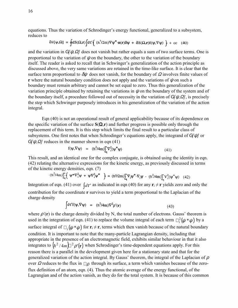
equations. Thus the variation of Schrodinger’s energy functional, generalized to a subsystem, reduces to

and the variation in G[ψ,Ω] does not vanish but rather equals a sum of two surface terms. One is proportional to the variation of ψ on the boundary, the other to the variation of the boundary itself. The reader is asked to recall that in Schwinger’s generalization of the action principle as discussed above, the very same variations are retained in the time-like surface. It is clear that the surface term proportional to δψ does not vanish, for the boundary of Ω involves finite values of r where the natural boundary condition does not apply and the variations of ψ on such a boundary must remain arbitrary and cannot be set equal to zero. Thus this generalization of the variation principle obtained by retaining the variations in ψ on the boundary of the system and of the boundary itself, a procedure followed out of necessity in the variation of G[ψ,Ω], is precisely the step which Schwinger purposely introduces in his generalization of the variation of the action integral.

Eqn (40) is not an operational result of general applicability because of its dependence on the specific variation of the surface S(ΩΩΩΩ,r) and further progress is possible only through the replacement of this term. It is this step which limits the final result to a particular class of subsystems. One first notes that when Schrodinger’s equations apply, the integrand of G[ψ] or G[ψ,Ω] reduces in the manner shown in eqn (41)

This result, and an identical one for the complex conjugate, is obtained using the identity in eqn. (42) relating the alternative expressions for the kinetic energy, as previously discussed in terms of the kinetic energy densities, eqn. (7)

Integration of eqn. (41) over ∫ 'τd as indicated in eqn (40) for any ri ≠ r yields zero and only the

contribution for the coordinate r survives to yield a term proportional to the Laplacian of the charge density

where ρ’(r) is the charge density divided by N, the total number of electrons. Gauss’ theorem is used in the integration of eqn. (41) to replace the volume integral of each term ( )ψψ *2

i∇ by a surface integral of ( )ψψ *i∇ for ri ≠ r, terms which then vanish because of the natural boundary condition. It is important to note that the many-particle Lagrangian density, including that appropriate in the presence of an electromagnetic field, exhibits similar behaviour in that it also integrates to ( ) ( )r'4/ 22 ρ∇m when Schrodinger’s time-dependent equations apply. For this reason there is a parallel in the development given here for a stationary state and that for the generalized variation of the action integral. By Gauss’ theorem, the integral of the Laplacian of ρ over Ω reduces to the flux in ρ∇ through its surface, a term which vanishes because of the zero-flux definition of an atom, eqn. (4). Thus the atomic average of the energy functional, of the Lagrangian and of the action vanish, as they do for the total system. It is because of this common

17

property that the variational properties of an atom are the same as those obtained for the total system. The zero-flux constraint, when applied to eqn. (42) also ensures that the atomic average of the kinetic energy is uniquely defined.

Using the result given in eqn. (43), the variation of G[ψ,Ω] as given in eqn (40), at the point of variation where Schrodinger’s equations apply, reduces to

The general result given in eqn. (44) is transformed into a statement of Schwinger’s principle of stationary action by restricting the subsystem to one which satisfies a particular variational constraint.

One considers the entire variation to be carried out using a trial function φ which, at the point of variation, reduces to the state function ψ. One imposes at all stages of the variational procedure, the constraint that the region Ω(φ), defined in terms of the trial function φ, be bounded by a “zero-flux surface”, one such that

where ρφ’ is the trial density. The region Ω(φ) represents the subsystem in the varied total system described by the trial function φ just as Ω(ψ) represents the subsystem in the state described by ψ. Requiring the fulfillment of eqn. (22) amounts to imposing the variational constraint that the divergence of '' φφ ρρ ∇⋅∇=∇ integrates to zero at all stages of the variation, ie,

for all admissible φ, which in turn implies that

The constraint in eqn. (47), that the variation of the integral of the Laplacian of ρ which includes a variation of its surface must vanish, results in an equating of the surface integral of the variation in the surface to the volume integral of the variation of the integrand to yield

and the RHS of this constraint equation can be substituted for the term involving the variation of the surface in eqn. (44). The RHS is easily evaluated to yield

where the final step uses Gauss’ theorem to replace the volume integral of a divergence with a surface integral. This is a most important step for because of it the imposition of the variational constraint yields only surface terms and thus Schrodinger’s equations are still obtained as the Euler equations from the volume variations. Using eqns. (48) and (49), the expression for the constrained variation obtained from eqn (44) is

18

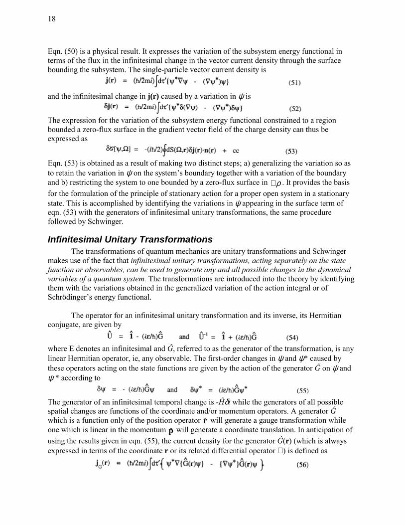
Eqn. (50) is a physical result. It expresses the variation of the subsystem energy functional in terms of the flux in the infinitesimal change in the vector current density through the surface bounding the subsystem. The single-particle vector current density is

and the infinitesimal change in j(r) caused by a variation in ψ is

The expression for the variation of the subsystem energy functional constrained to a region bounded a zero-flux surface in the gradient vector field of the charge density can thus be expressed as

Eqn. (53) is obtained as a result of making two distinct steps; a) generalizing the variation so as to retain the variation in ψ on the system’s boundary together with a variation of the boundary and b) restricting the system to one bounded by a zero-flux surface in ρ∇ . It provides the basis for the formulation of the principle of stationary action for a proper open system in a stationary state. This is accomplished by identifying the variations in ψ appearing in the surface term of eqn. (53) with the generators of infinitesimal unitary transformations, the same procedure followed by Schwinger.

Infinitesimal Unitary Transformations The transformations of quantum mechanics are unitary transformations and Schwinger

makes use of the fact that infinitesimal unitary transformations, acting separately on the state function or observables, can be used to generate any and all possible changes in the dynamical variables of a quantum system. The transformations are introduced into the theory by identifying them with the variations obtained in the generalized variation of the action integral or of Schrödinger’s energy functional.

The operator for an infinitesimal unitary transformation and its inverse, its Hermitian

conjugate, are given by

where E denotes an infinitesimal and Ĝ, referred to as the generator of the transformation, is any linear Hermitian operator, ie, any observable. The first-order changes in ψ and ψ* caused by these operators acting on the state functions are given by the action of the generator Ĝ on ψ and ψ * according to

The generator of an infinitesimal temporal change is -Ĥδt while the generators of all possible spatial changes are functions of the coordinate and/or momentum operators. A generator Ĝ which is a function only of the position operator r will generate a gauge transformation while one which is linear in the momentum p will generate a coordinate translation. In anticipation of using the results given in eqn. (55), the current density for the generator Ĝ(r) (which is always expressed in terms of the coordinate r or its related differential operator ∇ ) is defined as

19

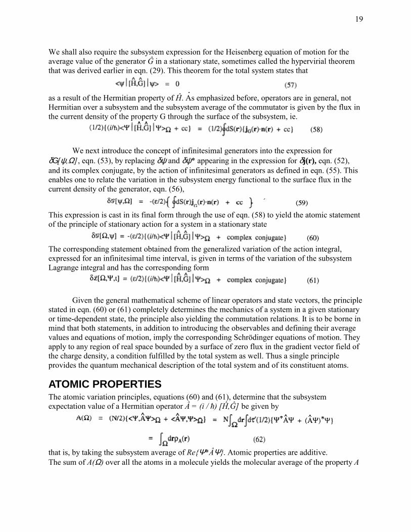
We shall also require the subsystem expression for the Heisenberg equation of motion for the average value of the generator Ĝ in a stationary state, sometimes called the hypervirial theorem that was derived earlier in eqn. (29). This theorem for the total system states that

as a result of the Hermitian property of Ĥ. As emphasized before, operators are in general, not Hermitian over a subsystem and the subsystem average of the commutator is given by the flux in the current density of the property G through the surface of the subsystem, ie.

We next introduce the concept of infinitesimal generators into the expression for

δG[ψ,Ω], eqn. (53), by replacing δψ and δψ* appearing in the expression for δj(r), eqn. (52), and its complex conjugate, by the action of infinitesimal generators as defined in eqn. (55). This enables one to relate the variation in the subsystem energy functional to the surface flux in the current density of the generator, eqn. (56),

This expression is cast in its final form through the use of eqn. (58) to yield the atomic statement of the principle of stationary action for a system in a stationary state

The corresponding statement obtained from the generalized variation of the action integral, expressed for an infinitesimal time interval, is given in terms of the variation of the subsystem Lagrange integral and has the corresponding form

Given the general mathematical scheme of linear operators and state vectors, the principle

stated in eqn. (60) or (61) completely determines the mechanics of a system in a given stationary or time-dependent state, the principle also yielding the commutation relations. It is to be borne in mind that both statements, in addition to introducing the observables and defining their average values and equations of motion, imply the corresponding Schrödinger equations of motion. They apply to any region of real space bounded by a surface of zero flux in the gradient vector field of the charge density, a condition fulfilled by the total system as well. Thus a single principle provides the quantum mechanical description of the total system and of its constituent atoms.

ATOMIC PROPERTIES The atomic variation principles, equations (60) and (61), determine that the subsystem expectation value of a Hermitian operator  = (i / ħ) [Ĥ,Ĝ] be given by

that is, by taking the subsystem average of ReΨ*ÂΨ. Atomic properties are additive. The sum of A(Ω) over all the atoms in a molecule yields the molecular average of the property A

20

The additivity applies to all properties, including those induced by an external field. As a consequence of the atomic force theorem to be derived below, the properties of an atom are determined by its distribution of charge, changing only in response to changes to its form in real space. Because of the zero-flux boundary condition, atoms are the most transferable pieces that can be defined in an exhaustive partitioning of real space. Thus atoms maximize the transfer of chemical information from one system to another. In those limiting cases where an atom can be transferred from one molecule to another without apparent change to its charge distribution, the atom contributes the same amount to every property in both systems and the result is a so-called additivity scheme. The theory of atoms in molecules recovers all experimentally observed cases of additivity, of volume, of moments, of energy, of polarizability and of magnetic susceptibility. The theory also predicts the measured change in the standard transferable energy exhibited by small ring systems, the strain energy. A single theory thus recovers the measurable consequences of the central concept of chemistry; that atoms and functional groupings of atoms exhibit characteristic sets of properties. We predict the behaviour of a substance in terms of the properties of the groups it contains and conversely, we identify the groups present in a substance through the observation of these same characteristic properties.

Atomic Theorems The mechanics of an atom in a molecule are determined by the atomic statements of the Heisenberg equation of motion, the atomic variation principles, equations (60) and (61). We shall summarize the atomic theorems obtained using the following generators in eqns. (60) and (61);

pˆ =G , generating a rigid translation of the coordinates of an electron over the basin of atom Ω and yielding an expression for the atomic force; pr ˆˆˆ ⋅=G , generating a scaling of the coordinates over the atomic basin and yielding the atomic virial theorem; rˆ =G , generating a gauge transformation to demonstrate the conservation of current as being a consequence of gauge invariance when the system is in the presence of a uniform constant magnetic field and to obtain the atomic current theorem.

The theorems determining the mechanics of an atom involve σ, the quantum mechanical stress tensor first introduced by Schrödinger,

In this case, the current density is a tensor and is obtained from eqn. (56) with pr ˆ)(ˆ =G . Properties refer to N electrons and Jp = Njp. The stress tensor, and hence the mechanics of a system, are determined by the information contained in just the first-order density matrix.

The properties of a subsystem are determined by fluxes in corresponding vector or tensor currents through its surface, contributions that are absent in the expressions for a total system of which the atoms are a part. These surface contributions arise from divergences of the same vector and tensor currents appearing in the local expressions for the mechanical properties of a system. Thus the study of the atomic theorems of force, energy and current lead to the formulation of a complementary set of expressions for the corresponding local properties of a system, all derived without the necessity of introducing ad hoc assumptions. Specific surface

21

properties can be of great importance. Poisson’s equation for example, enables one to equate the net charge on an atom or group to the surface flux in the electric field generated by the classical electrostatic potential within the group. The atomic current theorem equates the integral of the vector current density J(r) over the basin of the atom to its position weighted flux through the atomic surface. These two surface properties enable one to define atomic or group contributions to the polarizability and magnetic susceptibility.

The table in Appendix summarizes the atomic theorems for a number of important generators, including those to be derived below. In each case, the same theorem applies whether the spatial region denoted by Ω refers to the total system, in which case the surface integral vanishes, or to a proper open system, one satisfying the zero-flux boundary condition, eqn. (4). For a stationary state, the time-dependent term on the LHS vanishes and the first term on the RHS, the commutator average, is balanced by the associated surface flux term.

Atomic force theorem Setting the generator Ĝ(r) in cqn. (60) or (61) equal to p yields the time rate of change of the momentum, the atomic force theorem. The commutator average, Re(i / ħ)<[H,p]>Ω gives F(Ω), the Ehrenfest force acting over the basin of the atom. The variation in G[Ω,ψ] is determined by the surface term on the RHS of eqn. (33a) for the current jp, the surface integral of Rejp, eqn. (64). In a stationary state the basin and surface forces balance and the resulting expression relates the basin force to the negative of the pressure acting on every element of its surface, which is also the classical result,

or

The expression for the time rate of change of momentum of the density over the atom arises from an imbalance in the basin and surface contributions

where F(r,t), whose integral is F(Ω), is the force density

and Ψ denotes the time-dependent state function. The atomic force theorem demonstrates that the properties of a group in a stationary state, including the effects of external fields, are determined solely by the flux in the forces through its interatomic surfaces. There are no “through-space” effects in the quantum description of a subsystem. By preserving the interatomic surface characteristic of a given interaction, the properties of the group are preserved whether or not the bonded neighbour is considered to be present. Using this property it is not necessary to “cap” a group when wishing to study only a fragment of a larger system.

Atomic virial theorem The virial operator r · p has the dimensions of action and its time derivative is energy.

Setting the generator equal to pr ˆˆ ⋅ or its Hermitian form ( )rppr ˆˆˆˆ21 ⋅+⋅ yields the atomic

22

statement of the virial theorem. The commutator average yields twice the average electronic kinetic energy and the basin virial

The basin virial is the virial of the Ehrenfest forces acting over the basin of the atom (compare eqn. (39))

The variation in G[Ω,ψ] is determined by ReJr,p, eqn. (59), to yield the surface contribution --Vs(Ω), the virial of the forces exerted on the surface of the atom (compare eqn. (65))

where

The final surface integral in eqn. (70), which corresponds to a volume integral of the Laplacian density over the basin of the atom, vanishes because of the zero-flux boundary condition defining the atom. The surface integral Vs(Ω) has been shown to be proportional to the pressure volume product for the atom Ω. Thus this surface integral enables one to determine the pressure acting on an atom in any environment.

Equating the commutator and surface integrals, as required by eqn. (60) for a stationary state followed by some rearrangement, yields the atomic statement of the virial theorem

where the atomic virial V(Ω) is the sum of the basin and surface contributions. The use of eqn. (61) yields an expression for the virial of the force resulting from the change in momentum over the basin of the atom

By equating the electronic potential energy to the virial, one can define the electronic

energy of an atorn in a molecule Ee(Ω) as

When there are no external (Hellmann-Feynman) forces acting on the nuclei, the virial V equals the average potential energy of the molecule and Ee = T + V then equals the total energy of the molecule. Equation (74) is as remarkable as it is unique. It uses a theorem of quantum mechanics to spatially partition all of the interactions in a molecule, electron-nuclear, electron-electron and nuclear-nuclear into a sum of atomic contributions and the total energy of the molecule, as are all molecular properties, is given by a sum of atomic contributions

Remarkable as this definition of the energy of an atom in a molecule is, it would be of no

practical use if it did not exhibit the same degree of transferability from one molecule to another as does the atom itself, as previously illustrated in Fig. 3. As stated in the section listing the chemical constraints on the definition of an atom, if the atom appears the same in two different

23

systems, that is, if its distribution of charge remains unchanged on transfer, then all its properties must exhibit the same invariance. Correspondingly, if the charge distribution of the atom or group does change because of a changed environment, then the properties exhibit a corresponding degree of change.

Atomic continuity theorem The density operator ( )∑ −= i i rrˆ δρ and its associated number operator ( )∫= rrρˆ dN

are quantum observables: they are real dynamical variables which possess complete sets of eigenstates. Using the time dependent atomic variation principle, an atomic population is obtained as the expectation value of the observable N . The commutator of Ĥ and N vanishes, as does the corresponding variation in L[Ω,Ψ,t], and eqn. (61) yields the following integrated equation of continuity for the time-rate of change of an atomic population

Eqn. (76) describes the rate-of-change of the integrated atomic population and thus requires the presence of the term involving the change in the atomic surface with time.

Atomic current theorem When a system is in the presence of a magnetic field B and vector potential A(r) = (1/2)

B ×××× r, the single-particle current density is given by

where the generalized momentum ( )Ap ce+= ˆπ . The current and the magnetic properties it determines are independent of the origin, the gauge origin, chosen to define the vector potential A(r). This follows, because a change in gauge origin is equivalent to subjecting the state function and operators to a unitary transformation which leaves all observable properties unchanged. The generator of the transformation for a shift in origin of amount d is (1/2)(B ×××× d)·r, a constant times the electronic position vector r, and thus corresponds to a gauge transformation. The time rate-of-change of r is velocity and the commutator average in eqns. (60) or (61) with p replaced by π in the Hamiltonian, yields Π(Ω)/m, the atomic average of the velocity. This quantity equals J(Ω), the current in eqn. (77), averaged over the basin of the atom

The atomic variation principles have been shown to apply in the presence of an electromagnetic field and the variation in the atomic Lagrangian induced by the action of the generator r when equated to the RHS of eqn. (61) yields the atomic current theorem

Through the use of the identity

and Gauss’ theorem, eqn. (79) yields

24

Forming the dot product of the generator r with the vector (1/2)(B ×××× d) in eqn. (81) corresponds to subjecting the system to all possible gauge transformations. Since this result is obtained for all arbitrary variations, the quantity they multiply in eqn. (81) must separately vanish yielding the equation of continuity, eqn. (1). The use of the atomic variational principle for a stationary state yields eqn. (79) without the term dρ/dt, and the atomic current theorem states that the basin average of the current equals its position weighted flux through the atomic surface

Fig. 5. Displays of the trajectories of the induced current in benzene in the plane of the nuclei in a and for a plane 0.8 au above that in b for a perpendicularly applied field. The lower diagram is for the current induced in the LiH molecule for a field perpendicular to the plane of the diagram. Note that in benzene, trajectories encompass the entire molecule, while in LiH the majority of the trajectories are confined to the individual atomic basins separated by the interatomic surface indicated in the diagram.

25

Eqn. (61) also holds for all gauge transformations thereby ensuring, again through eqn. (59), conservation of the current for a system in a stationary state through the condition

Thus gauge invariance implies the equation of continuity or current conservation in a stationary state.

Placing a molecule in an external magnetic field induces a current within the molecule

and it is the magnetization density resulting from this induced current that determines the first-order response properties such as magnetic susceptibility χ and the nuclear shielding of NMR spectroscopy. In this situation the induced current replaces the electron density as the field of interest in the determination and understanding of the properties of the molecule. The flow of the density, the trajectories of the vector current field, induced in the benzene molecule for a field applied perpendicular to the plane of the molecule is displayed in Fig. 5. This very accurate display of the induced current (it satisfies the local condition of current conservation very closely) is itself a new development made possible by the use of the theory of atoms in molecules through the introduction of the use of multiple gauge origins in real space. In the IGAIM method (individual gauges for atoms in molecules) the gauge origin is placed at the nucleus of the atom for the determination of the atom’s contribution to the magnetic properties. In the CSGT method (continuous set of gauge transformations), a continuous set of gauge origins is used to calculate the induced current, one origin for each point in real space.

The presence of a ‘ring current’ is invoked in aromatic molecules in the explanation of

the exaltation and exceptional anisotropies observed in their magnetic susceptibilities and in the interpretation of NMR chemical shifts. The current induced by the application of an external magnetic field is a flow of electrons in physical space and its existence and properties are therefore, real and determinable. Thus the display of the current given in Fig. 5 provides a simple direct answer to the question as to whether or not a ring current is generated in benzene by a perpendicular field.

The existence of the ring current is further confirmed in the atomic contributions to χ .

An atomic contribution consists of one arising from the magnetization induced within the basin of the atom and another resulting from the flux in the induced current through the surface of the atom. In ionic and polar systems such as LiH whose current is also illustrated in Fig. 5, the induced current like ρ(r), is strongly localized to the individual atomic basins and the basin contributions to χ dominate. For benzene, which exhibits a significant ring current, the fluxes in the current through the interatomic surfaces of the carbon atoms in the ring far surpass the basin contributions, the same contribution being responsible for the observed anisotropy in χ . The contribution from a carbon atom to the shielding of its neighbouring proton demonstrates that the same ring current is responsible for the deshielding of an aromatic proton, as anticipated in the early shielding models.

Examples of Using Atomic Properties The theory of atoms in molecules enables one to investigate chemical models to

determine their validity and understand their atomic origins. To apply quantum mechanics to such problems, one simply extends the quantum description of the molecule to its constituent

26

atoms, without the use of any assumptions or models. The only approximation involved is in the determination of the wave function used in the analysis. The application of theory towards understanding the origin of specific chemical observations is illustrated for the concept of aromaticity.

To account for “aromatic exaltation” in χ , a carbon atom in benzene should have a

magnetic susceptibility greater than that of a correspondingly conjugated atom in a molecule assumed to be non-aromatic, carbon 2 in 1,3-cis butadiene for example. The value of χ (C) for benzene is found to exceed that for butadiene by 2.5 u where u denotes the unit –l x 10-6 emu mole-1. Six times this value, or 15 u, equals precisely the exaltation assigned to a benzene ring in the experimentally based additivity scheme of Pascal and Pacault. The contributions to χ from the hydrogens attached to these carbons in the two molecules are identical and the hydrogen atoms do not contribute to the exaltation. Not only does theory show that the exaltation arises solely from the carbon atoms in benzene but the relative values of the basin and surface flux contributions to χ (C) show that it is a consequence of the circular current flow that traverses the ring of carbon atoms for a field applied perpendicular to the plane of the nuclei.

The electron delocalization associated with the resonance model is also invoked to

account for aromatic stabilization. Accordingly, the benzene carbon atom should be more stable than the corresponding atom in butadiene and the theory of atoms in molecules shows this to be the case with the difference in their energies equaling -10.0 kcal mol-1. The hydrogen in butadiene possesses the greater electron population by a slight amount, and it is 3.5 kcal mol-1 more stable than H in benzene making the C-H group 6.5 kcal mol-1 more stable in benzene than in butadiene. Benzene is therefore, 39 kcal mol-1 more stable than six correspondingly conjugated acyclic C-H groups, a value comparable to the value of 36 kcal mol-1 quoted for the resonance energy of benzene. Having shown that theory recovers a given model, one may proceed to further analyze the atomic contributions to determine their physical origins. How is the resonance stabilization energy for example, related to electron delocalization? This is another property that is defined and determined by quantum mechanics within the theory of atoms in molecules and this question can be answered.

REFERENCES 1. E. Schrödinger, Quantisation as a problem of proper values, Ann. d. Phys. 79, 361

(1926). 2. P. A. M. Dirac, Physik. Zeits. Sowjetunion 3, 64 (1933). 3. P. A. M. Dirac, The principles of quantum mechanics, Oxford University Press,

Oxford, 1958. 4. R. P. Feynman, Space-time approach to non relativistic quantum mechanics, Rev.

Mod. Phys. 20, 367 (1948). 5. J. Schwinger, The theory of quantized fields. I, Phys. Rev. 82, 914 (1951). 6. R. F. W. Bader, A theory of atoms in molecules - a quantum theory, Oxford

University Press, Oxford, 1990. 7. R. F. W. Bader, Principle of stationary action and the definition of a proper open

system, Phys. Rev. B49, 13348 (1994).

27

8. R. F. W. Bader, Chemistry and the near-sighted nature of the one-electron density matrix, Int. J. Quantum Chem. 56, 409 (1995).

9. R. F. W. Bader and T. A. Keith, Properties of atoms in molecules: magnetic susceptibilties, J. Chem. Phys. 99, 3683 (1993).

10. R. F. W. Bader, P. L. A. Popelier and T. A. Keith, Theoretical definition of a functional group and the molecular orbital paradigm, Angew. Chem. Int. Engl. 33, 620 (1994).

11. R. F. W. Bader, S. Johnson, T.-H. Tang and P. L. A. Popelier, The electron pair, J. Phys. Chem. 100, 15398 (1996).

12. R. F. W. Bader and M. A. Austen, Properties of atoms in molecules: atoms under pressure, J. Chem. Phys. 107, 4271 (1997).

13. R. F. W. Bader and J. A. Platts, Characterization of an F-centre in an alkali halide crystal, J. Chem. Phys, 107, 8545 (1997).

28

Appendix