Federal Reserve Bank of New York

Staff Reports

Are Credit Default Swaps Associated

with Higher Corporate Defaults?

Stavros Peristiani

Vanessa Savino

Staff Report no. 494

May 2011

This paper presents preliminary findings and is being distributed to economists

and other interested readers solely to stimulate discussion and elicit comments.

The views expressed in this paper are those of the authors and are not necessarily

reflective of views at the Federal Reserve Bank of New York or the Federal

Reserve System. Any errors or omissions are the responsibility of the authors.

Are Credit Default Swaps Associated with Higher Corporate Defaults?

Stavros Peristiani and Vanessa Savino

Federal Reserve Bank of New York Staff Reports, no. 494

May 2011

JEL classification: G21, G33

Abstract

Are companies with traded credit default swap (CDS) positions on their debt more likely

to default? Using a proportional hazard model of bankruptcy and Merton’s contingent

claims approach, we estimate the probability of default for U.S. nonfinancial firms. Our

analysis does not generally find a persistent link between CDS and default over the entire

period 2001-08, but does reveal a higher probability of default for firms with CDS over

the last few years of that period. Further, we find that firms trading in the CDS market

exhibited a higher Moody’s KMV expected default frequency during 2004-08. These

findings are consistent with those of Henry Hu and Bernard Black, who argue that agency

conflicts between hedged creditors and debtors would increase the likelihood of corporate

default. In addition, our paper highlights other explanations for the higher defaults of

CDS firms. Consistent with fire-sale spiral theories, we find a positive link between

institutional ownership exposure and corporate distress, with CDS firms facing stronger

selling pressures during the recent financial turmoil.

Key words: credit derivatives, corporate bankruptcy, Merton’s distance to default

Peristiani, Savino: Federal Reserve Bank of New York. Address correspondence to Stavros

Peristiani (e-mail: steve.peristiani@ny.frb.org).The authors gratefully acknowledge the helpful

comments of Anna Kovner, Jennie Bai, Lin Peng, and Joao Santos. This paper benefited from

seminars at Baruch College-CUNY and the Federal Reserve Bank of New York. The authors also

thank Steven Burnett and Vitaly Bord for valuable research assistance. The views expressed in this

paper are those of the authors and do not necessarily reflect the position of the Federal Reserve

Bank of New York or the Federal Reserve System.

 

1  

1. INTRODUCTION

The wide-ranging financial reforms recently enacted by Congress have also focused on

how to regulate the complex over-the-counter global derivatives market. This proposed

legislation has fueled the long-standing debate over the appropriate regulatory framework for the

large and complex derivatives market. Title VII of the Dodd-Frank Wall Street and Consumer

Protection Act will effectively require that most derivatives be traded on centralized exchanges.

While the regulatory reform broadly targets all derivative instruments, the most important

derivatives contract under scrutiny after the recent financial meltdown is the credit default swap

(CDS).1

Since the inception of the credit derivatives market, market participants have underscored

its benefits in mitigating concentrations of credit risk, promoting diversification outside the

banking system, and enhancing trading liquidity. More recently, however, some policy makers

and financial commentators argue that CDS trading actually amplified risks in the recent

financial crisis (Stout 2009). One facet of credit derivatives trading that is often under intense

scrutiny is the “naked” CDS. Like any other naked trading position, this is a more speculative

transaction, because the CDS position is not used to hedge existing exposures to the underlying

asset.2

Besides these concerns, some argue that even if credit derivatives are used to insure

against existing credit risks, these hedges can engender agency problems between creditors and

debtholders and raise the likelihood of corporate bankruptcy. This issue has recently attracted

significant interest in the press and among finance and legal practitioners.3 Hu and Black (2008a,

2008b) formalize these agency problems, arguing that creditors who hedge their positions are

“empty creditors.” In addition to the pecuniary benefits of receiving interest and principal

payments, corporate debt owners also have legal rights that allow them to enforce lending terms

                                                            1 Stephen Fidler, Gregory Zuckerman, and Brian Baskin, “Swaps Come Under Fire — U.S. Regulators, European Leaders Seek More Oversight on Trades in Derivatives,” Wall Street Journal, March 10, 2010. 2 Wolfgang Münchau, “Time to Outlaw Naked Credit Default Swaps,” FT.com, February 28, 2010; Charles Davi, “Naked Credit Default Swaps: Exposed,” Atlantic, May 2009. 3 See, for example, “CDS Derivatives Are Blamed for Role in Bankruptcy Filings,” Financial Times, April 17, 2009; “YRC and the Street’s Appetite for Destruction,” Wall Street Journal, January 5, 2010; Daniel Gross, “Why GM May Go Bankrupt,” slate.com, May 12, 2009; Daniel Gross, “The Scary Rise of the Empty Creditor,” slate.com, April 21 2009; Caroline Salas and Shannon Harrington, “Darth Wall Street Thwarting Debtors with Credit Swaps,” Bloomberg, March 5, 2009; Andrew Ross Sorkin, “Is the Empty Creditor Theory Itself Empty?” NYTimes.com, December 21, 2009.  

 

2  

and take part in restructuring and bankruptcy proceedings. When debtholders hedge their

position with a CDS, they are able to “decouple” their economic and legal rights. Because they

are hedged, these creditors may not particularly care, or sometimes may even prefer, that the

company files for bankruptcy protection. Bankruptcy costs are generally very onerous; therefore,

any interference from an empty creditor can lead to an inefficient economic outcome for other

creditors, shareholders, and the firm, especially in cases where bankruptcy alternatives, such as

restructuring, are more efficient.

While the issue of empty-creditor conflicts between debtholders with CDS protection and

the debtor firm (henceforth referred to as the CDS firm) has attracted a lot of interest in the

financial press, other interpretations for any unusual rise in default risk among larger CDS firms

are possible. A higher default profile among CDS firms may not necessarily be triggered by

empty-creditor agency problems but may simply be caused by a rift in investor behavior and a

shift in credit sentiment in times of financial instability. In the aftermath of the recent financial

crisis, recent studies highlight a number of potential transmission mechanisms of distress across

markets that could indiscriminately drag down large and small companies alike. Shleifer and

Vishny (2011) and Hau, Lai, and Chua (2011) investigate the upsurge in fire sales of financial

assets as a catalyst for financial turmoil. Brunnermeier and Pedersen (2009) focus on the role of

margin financing in amplifying liquidity and funding problems and promulgating destabilizing

liquidity spirals. It is not difficult to envision under any one of these premises a scenario in

which default risks of CDS and non-CDS companies become displaced.

We formally investigate the relationship between credit derivatives and firm bankruptcies

using two distinct but related reduced-form methodologies to calibrate a firm’s default risk. The

first approach is a proportional hazard model that assesses a firm’s likelihood of filing for

reorganization over its entire public life cycle. The second approach measures corporate default

risks using Merton’s contingent claims model (Merton 1974). Merton’s distance-to-default

methodology provides a time-consistent indicator of corporate distress. The first phase of our

analysis relies on our own model-derived measures of implied distance-to-default scores to

assess the link between credit derivatives and firm default. In our second phase, we reestimate

this relationship using Moody’s KMV proprietary expected default frequency (EDF) measures,

which are also based on Merton’s approach to assessing corporate distress.

 

3  

Initially, we evaluate the impact of credit derivatives by using a binary indicator that

identifies firms with nontrivial CDS trading on their debt. We also decompose the effect of the

CDS indicator across years to better understand the effect of CDS over time. Our empirical

analysis reveals no significant link between CDS and the probability of bankruptcy over the

entire panel of U.S. nonfinancial public firms during 2001–08. However, when the effect is

decomposed by year, CDS firms exhibit a greater likelihood of default in 2008. In particular, the

odds ratio of the probability that a CDS firm will file for bankruptcy divided by the probability

that a similar non-CDS firm goes bankrupt surges to 2.57 in 2008.

The estimates of the bankruptcy hazard regressions are driven primarily by the relative

distribution of the bankruptcies among CDS and non-CDS firms and the fact that most of the

bankruptcy filings of CDS firms are clustered over the past few years. To avoid the lumpiness of

corporate bankruptcy events, we use Merton’s model to measure the relationship between

corporate distress and CDS. The relationship between implied default and the binary of indicator

CDS remains insignificant over the entire panel of U.S. nonfinancial firms. The distance-to-

default model estimates reveal again a significant increase in default among CDS firms over the

past few years, reinforcing some of the findings of the bankruptcy hazard regressions. Although

we observe Moody’s KMV corporate EDFs starting in 2004, by this metric of corporate distress

the regression results are more statistically significant in indicating a higher default risk among

CDS firms.

One possible limitation of the empirical analysis is that the observed positive correlation

between CDS and bankruptcy may be a case of reverse causality. In anticipation of problems,

creditors of the firm may buy protection in the period before bankruptcy and thus create this

spurious correlation. We use a two-stage approach to estimate an orthogonal instrument of

excess CDS exposure constructed to eliminate these reverse-causality problems. With this more

sophisticated approach, we continue to find a strong positive association between the firm-

specific index of excess CDS exposure and implied default.

The final phase of our empirical analysis investigates whether the apparent rise in default

risk experienced by CDS firms more recently is circumstantial, stemming from the unusual

fragility of the financial system. Existing theories describing deleveraging spirals and distressed

selling provide various mechanisms by which investors may be forced to sell their holdings when

stock prices plunge. In highlighting the importance of financial asset fire sales, Shleifer and

 

4  

Vishny (2011) note that institutions relying on short-term funding, such as the commercial paper

market, are more vulnerable during a financial crisis. Cella, Ellul, and Giannetti (2010) focus on

the intensity of institutional ownership to measure stock price selling pressures that could

increase volatility and amplify default risks.

We find a weak link between commercial paper funding and default, with firms relying

on this short-term financing exhibiting a slightly higher implied default. To be sure, we expect

these funding pressures to be more pertinent among asset-liability managed financial firms that

rely more heavily on these short-term sources to finance their activities. According to our

regression results, nonfinancial firms that are overly exposed to institutional ownership

experience higher default. Despite controlling for these alternative theories, however, we

continue to observe a strong positive link between excess CDS exposure and firm distress. The

findings are therefore consistent with all those alternative explanations that focus on the

importance of agency problems between creditors and debtors as well as the ferocity of the

recent financial crisis.

The remainder of this paper proceeds as follows. Section 2 briefly summarizes the empty-

creditor hypothesis, outlining the potential agency conflicts between debtholders with CDS

protection and debtors, as well as providing alternative explanations for the amplification of

corporate default risks. In section 3, we discuss the proportional hazard model of bankruptcy and

contrast it to Merton’s methodology. Section 4 describes the data sources and presents summary

statistics for the regression variables. Section 5 briefly documents the explosive growth of the

credit derivatives market. Sections 6 and 7 review our empirical evidence and analyze the

importance of CDS on corporate distress. In section 8, we develop an orthogonal instrument of

excess CDS exposure designed to eliminate reverse-causality problems. In section 9, we examine

more closely a number of competing explanations for the amplified default risks of CDS firms.

Section 10 summarizes our findings and presents concluding remarks.

2. MOTIVATION

2.1 Credit Derivatives and Agency Problems

The underlying economic intuition behind the empty-creditor concept is grounded on the

traditional principal-agent conflict theories formalized in the financial literature (Jensen and

Meckling 1976; Fama and Jensen 1983; Myers and Majluf 1984). In their earlier work

 

5  

highlighting the distortionary influence of credit derivatives, Hu and Black (2006, 2007) focused

mainly on equity ownership by developing the concept of the “empty voter.” Shareholders, in

effect, have economic ownership but also voting rights. Under normal conditions, firm

shareholders are expected to exercise their voting rights to optimize the value of their equity

holdings. Hu and Black point out that a credit derivatives position can weaken the incentives to

use voting rights to safeguard economic ownership.

The empty-creditor concept is a similar agency problem because debtholders with CDS

have a direct mechanism for influencing a firm’s decision through noneconomic rights, such as

voting on the restructuring or bankruptcy-related decisions and the exercise of covenants. Credit

derivatives and other financial innovations, such as collateralized debt obligation securities,

allow debtholders to cushion or entirely eliminate the economic exposure of losing principal and

interest while maintaining valuable noneconomic rights. Moreover, debtholders can benefit from

a negative economic ownership that arises if their hedge is higher than their principal debt

exposure.

The empty-creditor premise has been met with a lot of skepticism from participants in the

credit derivatives and fixed-income markets. A recent research paper of the International Swaps

and Derivatives Association (ISDA) questions the validity of the empty-creditor hypothesis on

logistical grounds (Mengle 2009). This paper argues that CDS hedging strategies cannot be

exploited systematically because the market would anticipate and incorporate much of the credit

risk and thus make such positions prohibitively expensive to protection buyers.

More recently, Bolton and Oehmke (2009) take a careful look at this issue by developing

a theoretical limited-commitment model. The authors show that, at least initially, CDS enhance

value by strengthening incentives for borrowers to engage in positive net-present-value projects,

raising the likelihood that they can repay their obligations. In a limited-commitment setup, where

the borrower is not always bound to pay its debt, the presence of CDS forces debtors to increase

investment and lowers strategic default. However, with creditors opting to increase their credit

protection using CDS to insure their exposures more effectively, these amplified positions

generate empty-creditor conflicts.

Ashcraft and Santos (2009) investigate whether credit derivatives have lowered the cost

of debt financing for corporations. The authors identify two channels through which CDS trading

could reduce such costs. A CDS can ultimately help lenders hedge their underlying exposure to

 

6  

borrowers. Moreover, the CDS market could also lower the cost of debt by increasing

information on traded firms and enhancing price discovery. More important, this study also

highlights a downside to credit derivatives trading, pointing out that it may allow lenders to

hedge their credit exposures after the loan has been granted in a way that is unobservable to the

firm and outside investors. A consequence of CDS hedging is that banks insured against a direct

exposure to borrowers would have reduced incentives to monitor these firms ex post.

This reduction-in-monitoring hypothesis is closely associated with the empty-creditor

hypothesis in many ways. The agency problems are more threatening in the latter hypothesis,

however, because hedged creditors are not only uninterested in monitoring but also stand to

benefit if the firm files for bankruptcy. Ashcraft and Santos (2009) find no evidence that CDS

firms experience lower credit spreads when issuing in the bond market or syndicated loan

market. Instead, their findings suggest that the onset of CDS trading has adversely affected the

financing costs of riskier firms as well as those that are more informationally opaque.

Most of the empirical support for the empty-creditor hypothesis is anecdotal in nature,

based on reported cases of corporate distress in which a firm with existing CDS contracts was

arguably forced into bankruptcy. A recent Economist article highlights several bankruptcies

blamed on bondholders that had unusual economic exposures (cases included Six Flags,

AbitibiBowater, General Growth Properties, and General Motors).4 Morgan (2009) reports the

more recent struggles of Gannet Co. to navigate through a difficult financial period, while

apparently facing intense pressure from hedged CDS debtholders. Bolton and Oehmke (2009)

provide a table summarizing several potential incidences of the empty-creditor problem over the

past few years.

From all the examples cited above, the bankruptcy of AbitibiBowater is one of the most

interesting cases because it highlights all facets of the agency-problems gamesmanship between

creditors and the debtor. Bowater merged with Abitibi in a leveraged buyout in 2008; burdened

by excessive debt, the company wanted to exchange its 9 percent bonds to improve cash flow to

ward off bankruptcy. To complete this exchange, the company needed 97 percent acceptance

from bondholders. In the end, the company was able to get a 54 percent approval. The failure to

                                                            4 “No Empty Threat: Credit-Default Swaps Are Pitting Firms against Their Own Creditors,” Economist, June 18, 2009, page 79. 

 

7  

restructure its debt was largely attributed to bondholders with large CDS positions, who stood to

benefit from the company’s bankruptcy.

The struggle between hedged bondholders and AbitibiBowater was actually more action

packed. On March 20 2009, with their expiration getting closer to maturity, CDS holders lobbied

to have AbitibiBowater default on its obligations. To avoid these pressures, AbitibiBowater

obtained a court order enabling it to suspend bond payments while working through its

restructuring. Running out of time, CDS holders stood to lose close to $500 million. An ISDA

ruling on March 28, however, gave CDS holders the right to backdate their claim through a cash-

auction system, essentially validating their default claims.

2.2 Alternative Hypotheses for Rising Default Risks among CDS Firms

While these agency problems between insured debtholders and debtors outlined above

offer an interesting interpretation, other explanations could also account for an increase in default

among CDS firms. A higher default profile among larger CDS firms may not be associated with

misaligned incentives between insured creditors and debtors but could be simply circumstantial,

caused by a fundamental change in credit sentiment in an economic crisis. Shleifer and Vishny

(2011) assert that fire sales of financial assets during a crisis could be a possible transmission

mechanism of distress across both large and small firms. Under this mechanism, forced sales by

distressed financial firms or investors could trigger a cascade of fire sales that spread to other

institutions and affect not only the creditworthiness of smaller and more vulnerable non-CDS

companies but also bigger CDS corporations.

Several studies in the financial literature argue that investors with shorter trading

horizons, such as hedge fund investors and certain institutional investors, might be more

predisposed to sell during a financial panic, driving stocks below their fundamental value (De

Long, Shleifer, Summers, and Waldman 1990). Brunnermeier and Pedersen (2009) argue that the

perils of margin financing can be amplified by market and funding liquidity problems and lead to

destabilizing liquidity spirals. Cella, Elul, and Giannetti (2010) find that short-term investors

sold more stocks than long-term investors after the collapse of Lehman Brothers. Arguably, one

might expect long-term investors to hold a relatively higher fraction of larger CDS firms in their

portfolios. In this case, a fire sale by short-term investors should be more detrimental to smaller

companies and in theory lead to a widening default premium between CDS and non-CDS firms.

 

8  

3. MODELING FIRM DEFAULT

The primary focus of our empirical analysis is to investigate the relationship between

CDS and the likelihood of debtor default. We use two approaches to measure corporate distress.

The more direct method is a reduced-form hazard regression model of bankruptcy. Terminal

events such as bankruptcy are not uncommon in the life of a corporation. Over the entire sample

period 2001–08, there were more than 520 corporate bankruptcies for publicly traded U.S.

nonfinancial corporations included in Compustat. This fairly large sample shrinks substantially

when we focus on CDS firms, which experienced only 43 bankruptcies. This smaller number of

bankruptcies could be more challenging because much of the proportional hazard analysis is

predicated on the relative frequency of these events across CDS and non-CDS firms. To improve

statistical power, we investigate an alternative measure of firm distress derived from Merton’s

model. In contrast to the bankruptcy approach, these implied measures of default are fully

observable over the entire life cycle of the firm.

3.1 A Proportional Hazard Model of Bankruptcy

Several academic papers have proposed various reduced-form approaches to modeling

corporate bankruptcy. Early studies relied primarily on accounting variables to predict the

probability of bankruptcy (Altman 1968; Ohlson 1980). Altman’s original study uses

discriminant analysis to develop firm Z-scores that are widely used in the academic literature and

by practitioners to evaluate corporate distress. Recent studies propose a dynamic cross-sectional

time-series logit model to estimate the conditional probability of bankruptcy (Shumway 2001;

Campbell, Hilscher, and Szilagyi 2008). Our empirical analysis investigates firm distress using a

hazard model to compare the bankruptcy rate of CDS and non-CDS firms. This methodology,

which offers a convenient framework for analyzing credit risk over the entire life cycle of public

firms, has been extensively applied in the financial literature. Chava and Jarrow (2004) provide a

broad comparison of the forecasting efficiency of these various bankruptcy models.

The actual termination event in the hazard regression model is firm bankruptcy. We use a

proportional hazard framework to analyze the default rate of corporate debt securities. Assume

that i denotes a random variable representing the time to bankruptcy for company (i). The

hazard rate is defined as the probability that the firm files for bankruptcy in the next period,

given that it has not done so up to now. More formally, the bankruptcy rate can be defined as

 

9  

i ii t 0

P(t t t | t)(t) lim .

t

(1)

The basic proportional hazard framework asserts that

i it( ) h( )exp(z ). (2)

The vector itz represents the vector of exogenous variables affecting firm bankruptcy.

The function h( ) is commonly referred to as the baseline hazard function. Essentially, the

proportional hazard specification is a semiparametric method of estimation that conditions out

the baseline hazard and focuses on the proportionality factor tiexp(z ) to estimate the influence

of the explanatory variables.

We can rewrite equation (2) to formalize our general hypothesis of testing the influence

of CDS on the bankruptcy. In particular, the model can be specified as

i 0 1 t 2 SIC t 1,i ti( ) h( )exp( I I x CDS ). (3)

The explanatory variable tI is a dummy variable controlling for time variation, while SICI

measures industry effects at the one-digit SIC level. The lagged explanatory vector t 1,ix

controls for variation observed across the panel of firms. Finally, the variable tiCDS represents a

binary indicator of firms with outstanding CDS on their debt. This specification allows us to test

the following general hypothesis.

Hypothesis 1: A positive and statistically significant coefficient on would be consistent

with empty-creditor agency problems between creditors and the debtor firm, indicating that CDS

increase the bankruptcy rate.

Hypothesis 1 is a broad test of the empty-creditor premise, which asserts that CDS firms

exhibit a higher default over the entire sample period. In reality, the CDS dummy variable is just

a simple proxy for potential empty-creditor problems and does not fully capture the underlying

composition of the protection buyers and the intensity of the empty-creditor problem. In theory,

agency problems will be greater if the protection buyers are existing bondholders —potential

empty creditors—as opposed to other nonvoting investors and dealers taking a short position on

the company’s credit. Ideally, we would want to control for the intensity of the CDS (for

instance, the volume of existing CDS relative to outstanding debt) and the distribution of

 

10  

protection buyers, particularly whether they are creditors or not. Unfortunately, this information

is not historically available at the company level.

Another possible limitation of the specification defined by equation (3) is that it assumes

that agency problems between creditors and borrower would manifest over the entire 2001–08

period. To be sure, these conflicts were evident even in the earlier part of our sample period. The

first such case reported in the financial press was Marconi Corporation’s effort to restructure in

2001. This struggling U.K. telecommunication company faced unyielding members of the bank

syndicate that refused to agree to any restructuring unless it was formally classified as a credit

event under ISDA rules. The potential for empty-creditor conflicts was formally discussed in a

2006 report published by an association of solvency professionals, which detailed the impact of

credit derivatives on restructuring and bankruptcy.5

It is plausible that empty-creditor hedging strategies might have surfaced more gradually

as participants in the CDS market became more sophisticated and developed more complex

strategies. Bolton and Oehmke (2010) demonstrate that the intensity of the agency conflicts are

likely to be much higher when creditors take larger bets and overinsure against the debtor. Their

theoretical findings suggest that debtor-creditor conflicts would be prevalent in a market with

widespread use of the credit derivatives products. Moreover, these conflicts would be magnified

in financial downturns, because the higher incidence of corporate distress would increase the

value of the CDS contract.

To capture this possible incremental effect of credit derivatives on the likelihood of

corporate distress, we modify the regression specification defined by equation (4) to include the

interaction of yearly dummy variables tI with the CDS binary indicator. In particular,

2008

i 0 1 t 2 SIC t 1,i t ti tt 2001

( ) h( ) exp( I I x CDS I ).

(4)

This specification leads to the following hypothesis.

Hypothesis 2: A positive and statistically significant coefficient on t

(t 2001, , 2008) is consistent with the presence of empty-creditor agency problems between

creditors and debtor firms in that particular year t.

                                                            5 See “Credit Derivatives in Restructurings: A Guidance Booklet,” INSOL International, 2006. http://www.insol.org/page/60/credit-derivatives-in-restructuring. 

 

11  

3.3 Merton’s Contingent Claims Approach

In his seminal paper, Merton (1974) models a firm’s equity as a call option on the value

of assets. The strike price of the option is determined by the firm’s contractual liabilities. Crosbie

and Bohn (2001) outline a calibration method that constructs a distance-to-default (DD) measure

from the underlying Black-Scholes option-theoretic model proposed by Merton. Several studies

use Merton’s model to estimate the probability of default for nonfinancial firms (Vassalou and

Xing 2004; Bharath and Shumway 2008; Campbell, Hilscher, and Szilagyi 2008). Park and

Peristiani (2007) apply this same methodology to determine the probability of the failure of

publicly traded banks. In a nutshell, the Merton model can be represented by a two-equation

system:

rTEti Ati 1ti ti 2tiV V N(d ) e L N(d ), (5)

and

AtiEti 1ti Ati

Eti

VN(d ) .

V (6)

The variable EtiV denotes the i-th firm’s market value of equity at period (t) , AtiV represents the

market value of assets, and tiL is total debt, which corresponds to the exercise price. Consistent

with the Black-Scholes framework, AiV is assumed to follow a geometric Brownian process

with drift and volatility Ati . Similarly, the variable Eti denotes the volatility of firm equity,

tr is the risk-free interest rate, and T is time to expiration. The Black-Scholes distance terms are

defined by 21ti Ati ti t Ati Atid [ln(V L ) T(r 0.5 )] T and 2ti 1ti Atid d T .

As described by Crosbie and Bohn (2001), this nonlinear two-equation system can be

solved to derive estimates of AV and A using known values for EV , E , and debt.6 Based on

these estimates, the distance to default at period t is given by

2

Ati ti Atiti

Ati

ln(V L ) T( 0.5 )DD .

T

(7)

                                                            6 To solve the nonlinear system of two unknowns and two equations, we used the SAS PROC MODEL procedure.

Estimates for the firm’s asset value Ait(V ) and volatility Ait( ) were solved using Newton’s nonlinear

approximation technique.

 

12  

In line with most studies in the literature, we assume a yearly framework ( T 1 ), and itL is

measured by debt obligations with one-year maturity plus half the longer-term debt (debt

maturing after one year). Following Campbell, Hilscher, and Szilagyi (2008), the drift parameter

is estimated by 0.06 r where the risk-free is measured by the three-month Treasury bill rate

and the value 0.06 represents the equity risk premium.7 For our purpose, there is no need to

adjust tiDD because it provides a time-consistent indicator of solvency over the life cycle of the

firm. Thus, our structural Merton distance-to-default estimate is appropriate for investigating the

hypothesis that CDS amplify agency problems between creditors and debtors.

Merton’s method has been applied extensively in the recent financial literature to

estimate corporate default and is the foundation for Moody’s KMV model (Kealhofer 2003).

Instead of relying on our derived measures of default, we choose to use the KMV EDFs as a

proxy for corporate distress. Moody’s KMV uses a large proprietary database of defaults to

calibrate the EDFs to the historical experience.

To tests the implications of a CDS in the Merton method, we need to formally define an

econometric model for the determinants of itDD . Admittedly, this “reverse engineering”

approach is an unusual exercise because, as described above, the gist of Merton’s methodology is

to calibrate solvency risks based on a handful of key factors (market value of equity, face value

of debt, equity volatility, and risk-free rate). If the Merton approach were not available, a simple

alternative would have been to gauge corporate distress by the firm’s stock volatility (effectively

the key input in Merton’s model). However, if we can model the underlying factors that

influence firm volatility, it follows by the same logic that we can also use a regression

specification to understand the determinants of the implied measure of default (in addition to the

known inputs used in Merton’s calibration).

Our analysis investigates the most straightforward relationship between Merton’s tiDD

measure of debtor default and the presence of CDS. A company’s distance to default is assumed

to vary over time and across industry and generally be determined by firm-specific factors,

including, of course, equity volatility and the debt ratio. More precisely, the model is defined as

                                                            7 Studies in the literature have proposed different ways to estimate the drift. For instance, Vassalou and Xing (2004) estimate based on the firm’s equity return. This approach is more difficult in a panel with a shorter time dimension

as it is more likely to yield noisier and less efficient estimates of the drift.

 

13  

ti 0 i 1 t 2 SIC t 1,i ti tiDD I I x CDS . (8)

This model is very similar to the parametric component of the hazard regression, with the

exception that now the specification includes a fixed-effects regressor to absorb all the

unobserved heterogeneity among firms. This specification tests again the general premise

defined by hypothesis (1). In the current framework, a negative and statistically significant

coefficient on would suggest the presence of empty-creditor agency problems between

creditors and the debtor firm, in the sense that the CDS decreases the distance to default and

brings the firm closer to default.

We also examine a weaker form of this hypothesis estimated by the model

2008

ti 0 i 1 t 2 SIC t 1,i t ti t tit 2000

DD I I x CDS I .

(9)

This more flexible specification asserts that these agency conflicts manifest under certain

economic conditions. A negative and statistically significant coefficient on t

(t 2000, , 2008) would indicate the presence of empty-creditor agency problems between

creditors and debtor firms in year t.

4. DATA

This study uses several sources of information to identify firms with existing CDS trades

and investigate the bankruptcy rate and distress risks of publicly traded companies. The primary

source for firm-specific information is the Compustat database. To measure stock market

performance, we use information from the Center for Research in Security Prices (CRSP) daily

stock file. These two primary data sources were complemented with additional firm-specific

information from Capital IQ.

We relied on several sources to formally identify firms that filed for bankruptcy

protection (Chapter 11 and 7). Most of our information on bankruptcies during the period 2001–

08 is derived from SDC Platinum and Capital IQ. Together, SDC Platinum and Capital IQ

provide an extensive list of bankruptcies going back to the 1980s. To fill some occasional gaps in

these two databases, we also used information from the Moody’s Default Database and the

CRSP delisting header file. In the case of the latter, we identified as bankruptcies only those

 

14  

firms with a delisting code of 574. In the Moody’s Default Database, we considered only

defaults that had an explicit bankruptcy type code.

It is important to emphasize that the terminal default events are limited to bankruptcies

but exclude restructurings.8 In the U.S. CDS market, restructuring was not typically considered a

trigger event for speculative-grade single-name reference entities. However, restructuring was

often included in the list of possible credit events for investment-grade contracts. In spite of these

conventions, Altman and Karlin (2009) point out that there was a recurring ambiguity in

deciding whether debt-exchange restructurings could trigger a payout. Even though a

restructuring was often included in the menu of credit events, the general practice was not to

consider it a trigger for default. The difficulty with enforcing restructuring as a credit event was

that ISDA documentation specified that this event be binding on all parties; in practice,

restructuring is typically binding only on investors that accept its terms. In 2009, ISDA formally

resolved this ambiguity by ruling that these restructuring events do not constitute a default event

trigger.

Although technically foreign companies can file for bankruptcy in U.S. courts, we limited

the sample of public companies to U.S. domiciled firms. Because our information traces

primarily U.S. bankruptcies, we cannot fully account for the possibility that a foreign company

may have filed for bankruptcy in its home country or in some other overseas jurisdiction. In

addition to dropping foreign firms, we also eliminated any firm with missing values for assets,

all financial firms (that is, firms with SIC codes in the range 6000–6999), and utility companies

(SIC codes in the range 4900–4999). The final sample traces the financial performance of a panel

of U.S. nonfinancial firms during the period 2001–08.9

We identified CDS firms in the sample by using the Markit CDS Pricing Database.

Markit was founded in 2003 after the company entered into agreements with nearly all large

market participants to establish a reference entity database to enhance liquidity, transparency,

and standardization in the credit derivatives market. Currently, Markit provides CDS spread

                                                            8 As shown by Altman and Karlin (2009), the majority of firm restructurings eventually drift into bankruptcy. Thus, even though these restructurings are not initially considered as defaults, they subsequently appear in our bankruptcy sample a few years later. 9 A major complication with financial firms is that often the resolution process is taken over by the regulator. These potential empty-creditor problems are therefore obfuscated by the presence of the regulatory agency. For instance, the insolvent insurance company Ambac Assurance was recently forced to undergo an intricate reorganization that included a partial takeover by its regulatory authority. Even so, ISDA classified Ambac’s failure as a bankruptcy instead of a restructuring event, triggering a payment to CDS protection buyers of Ambac’s bonds.  

 

15  

information on most corporations with nontrivial CDS trading (around 3,000 firms and

sovereigns). Markit’s coverage of the earlier period is also quite broad, covering most companies

with CDS trades (in 2002, the coverage included roughly 1,400 companies and sovereigns).

Despite the long historical coverage, the Markit database does not include every company

with CDS trading. Markit acknowledges that a small fraction of traded reference entities might

not be reported because information on market participants is not adequate for construction of an

accurate composite measure of CDS spread. The undisclosed information on these CDS firms

raises concerns about sample bias, as many of them will be included in the non-CDS sample.

However, the misclassification of CDS firms as non-CDS firms would actually work against the

null hypothesis that credit derivatives contribute to higher default.

Markit provides exact information on the existence of an outstanding CDS contract on

the firm’s dollar-denominated senior unsecured debt. Markit uses its unique tickers to identify

companies that do not always correspond to the official company equity ticker. To compensate

for these discrepancies in tickers, we manually matched each U.S. firms’ CDS ticker in Markit to

its actual exchange ticker using Capital IQ. Finally, to ensure the accuracy and completeness of

the Markit CDS population, we compared this information to a smaller list of companies with

CDS trading available from Bloomberg and the Depository Trust and Clearing Corporation

(DTCC). 10

Last, a key variable in our analysis examining the public life cycle of a company is firm

age. To determine the age of the public firms in our sample, we use information from the New

Issues Database from SDC Platinum. That database contains information on most initial public

offerings (IPOs) in United States starting in the mid-1980s. For the more mature firms that were

in existence before the 1980s, the missing IPO date was filled with origination date from the

CRSP header file.

                                                            10 Markit as well as Bloomberg uses dealer quotes to construct its composites. It is quite plausible therefore that a reported CDS spread may not necessarily reflect a trade. Our analysis presumes that, when dealers are making market on a firm, some trades have been executed at some point in the past. Using DTCC information, we were able to identify about 250 nonfinancial U.S. firms with existing gross notional CDS positions in 2009. Of the largest 100 companies in our sample, most of those identified as CDS firms have a reported outstanding gross notional volume. Nearly all of these top 100 firms not in the DTCC list are large technology firms (Microsoft, Google, Apple, etc.) that have very little debt and therefore should not have made the cutoff. Consistent with these findings, we find that all large non-CDS on the largest 100 list were not included on the DTCC list. This quick comparison suggests that firms reported in the Markit database have existing traded CDS positions on their debt.

 

16  

4.1 Description of Explanatory Variables

The specifications examining the determinants of the distance to default and bankruptcy

rate are closely related. Both models control for time effects, industry effects, and stock

exchange listings. For the most part, the explanatory vector t 1,ix controls for firm

characteristics, is also very similar in both default models. These specifications also allow for the

possibility that the default or bankruptcy rate will likely vary over the life cycle of the firm,

rising as the firm matures but then declining after the firm reaches some optimal scale. One

advantage of the proportional hazard model is that it intrinsically captures this nonlinearity in

bankruptcy rates. In the distance-to-default specification, the concavity of the default probability

is captured by including the age of the firm (AGE) and AGE squared as explanatory variables.11

A key determinant of corporate distress is firm size (SIZE), measured by the logarithm of

total market capitalization. We considered various accounting variables in our regression

analysis. The regression models include several financial ratios used in the earlier bankruptcy

literature. The ratio of working capital to total assets (WORKING_CAP) gauges a firm’s capital

adequacy. The specifications take account of the firm’s ability to generate sales and profits by

controlling for the EBITDA-to-assets ratio (EBITDA_ASSETS), the total sales-to-assets ratio

(SALES_ASSETS), and the ratio of cash assets (CASH_ASSETS).

Shumway (2001) demonstrates that market-based measures of firm performance are

useful predictors of bankruptcy. A key indicator of firm riskiness in both the default and the

bankruptcy models is stock volatility (STOCK_VOLATILITY). In addition, a firm’s abnormal

stock return is a good proxy for idiosyncratic risk (STOCK_RETURN). We computed annual

measures of stock volatility for each firm (measured by the standard deviation of daily returns).

Similarly, we estimated STOCK_RETURN as the average yearly abnormal stock return (firm

stock return minus the value-weighted total market CRSP return). In addition to market-derived

variables, the models include firm valuation, which is defined as the market value divided by the

book value of assets (MARKET_BOOK). This variable is a simplified version of the q ratio that

could reflect a firm’s franchise value and capture its potential growth prospects.

Leverage is also an important trigger of default. To assess the effect of corporate debt

structure, the models control for the debt-to-assets ratio (DEBT_ASSETS). Gilson, John, and

                                                            11 The variable AGE is measured from the time of IPO. For firms with missing IPO dates, the baseline for age is its first public listing reported in the CRSP header files.

 

17  

Lang (1990) point out that firms with complex debt structures—that is, a wide variety and

classes of debt—are less likely to resolve through a restructuring. To investigate the role of debt

complexity, the preliminary specifications also examined the effect of the loan-to-debt ratio and

a Hirschman-Herfindahl concentration measure of debt structure. Overall, these corporate debt

structure variables were not statistically significant and therefore were omitted from the final

specification.12

To reduce the influence of outliers, we winsorized all firm-specific explanatory variables

at the 1st and 99th percentile values computed over the entire sample period of 2001–08. Table 1

summarizes the sample means for all the continuous explanatory variables for CDS and non-

CDS companies. The table illustrates again the considerable size gap between CDS and non-

CDS firms. CDS firms are more mature, with an average life of 25.6 years compared to 12.9

years for the non-CDS firms. While larger CDS companies are generally less risky and exhibit

less volatility, they also garner significantly smaller abnormal stock returns. Non-CDS firms

maintain higher working capital ratios and cash-to-asset ratios to compensate for their greater

risk profile.

5. THE RAPID GROWTH OF THE CREDIT DERIVATIVES

Banks first introduced credit derivatives in the early 1990s to lower exposure to corporate

credit risk. Beginning in 2002, credit derivatives attracted greater interest from institutional

investors and hedge funds and reached over $62 trillion in notional market outstanding by the

end of 2007 (figure 1). Indexed CDS were a key contributor to the high growth in the mid-2000s.

In contrast to “single name” CDS, these indexes offer protection against a group of equally

represented corporate entities (typically, 125 corporate names). This explosive growth of the

credit derivatives market suggests that the intensity of debtor-creditor problems might have risen

more incrementally during this period. As shown by figure 1, in 2000 the existing volume of

credit derivatives amounted to roughly 9.7 percent of the total outstanding value of international

debt securities. By 2007, this ratio surged to over 270 percent.

Table 2 presents the growth of the CDS market by tracing the number of U.S. domiciled

nonfinancial public firms with traded positions as of January 2001. Despite the relatively small

                                                            12 Information on the debt breakdown is available from Capital IQ. We decomposed total debt into six categories (term loans, revolving credit, senior bonds, subordinated bonds, commercial paper, and other debt). Based on these categories, we calibrated a firm’s degree of debt complexity by using a simple Herfindahl-Hirschman index formula.

 

18  

volume of notional volume outstanding in the early 2000s, many of the large public U.S.

companies were trading in the credit derivatives market. The table also documents a wide size

differential between these two groups of firms. The average CDS firm was more than 20 times

larger than the average non-CDS firms during this period. Figure 2 shows that smaller firms are

unlikely to attract any significant interest from CDS buyers. Despite the considerable size gap

between these two subsets of companies, companies with outstanding credit derivatives show

significant heterogeneity. For instance, about half the firms located in the 90th percentile of asset

size have existing CDS contracts on their debt. The diversity in CDS coverage among large firms

is very useful in assessing the importance of agency problems between creditors and debtors.

6. THE IMPACT OF CDS ON THE BANKRUPTCY RATE

The first stage of our empirical analysis investigates the relationship between corporate

bankruptcy and credit derivative contracts. Table 3 presents the evolution of the unconditional

bankruptcy rate for CDS and non-CDS over the entire sample period. The number of smaller

non-CDS firms declines steadily over the 2001–08 period because of the large wave of

consolidations through mergers and acquisitions in the latter half of this period. In contrast, the

number of CDS firms rises gradually, with credit derivatives becoming a popular contract among

banks and institutional investors.

In total, 43 bankruptcies occurred among CDS firms over the entire sample period,

amounting to about 6.4 percent of cumulative bankruptcies. Non-CDS firms experienced 480

bankruptcies, corresponding to close to 14 percent of the cumulative bankruptcy rate. The bulk

of bankruptcies for CDS companies occurred primarily over the last few years of the sample. In

comparison, bankruptcies of non-CDS firms are clustered in the earlier part of the sample period,

following the dot-com collapse and the economic downturn in 2001. It is noteworthy that the

bankruptcy rate for large CDS firms in 2008 is 3.42 percent, significantly greater than the 1.23

percent rate experienced by non-CDS firms.

The specifications reported in the first and second columns in each panel of table 4 are

defined to test hypothesis 1 and 2, respectively. At the bottom of the table, we report the

likelihood ratio 2 statistics for the hazard regressions. The strong significant values of the

likelihood ratio statistics indicate that all the hazard specifications fit the data very well. We

generally observe a strong link between market-based explanatory variables and the conditional

 

19  

probability of bankruptcy. The positive and negative patterns of significant coefficients on the

quadratic terms of log(MARKET_CAP) signify a concave relationship between firm size and

bankruptcy. This concave relationship is consistent with the Gilson, John, and Lang (1990)

paper, which argues that larger companies with more complex debt structures will be more

inclined to file for bankruptcy. This pattern of rising likelihood of default, however, eventually

dissipates for larger and safer corporations.

Firms with higher values of stock volatility exhibit a significantly greater likelihood of

filing for bankruptcy, while better-performing firms with larger excess returns are less likely to

file. Consistent with the previous bankruptcy literature, we find that accounting variables that

measure profitability and capitalization are also strong determinants of firm survival. The

significant negative effect of WORKING_CAP confirms that better capitalized companies are

less likely to become insolvent. The estimates also reveal that firms with higher franchise value,

measured by MARKET_BOOK, exhibit a lower likelihood of bankruptcy.

More important, the effect of the CDS dummy variable over the entire panel of firms is

positive but insignificant (first column of table 4), indicating no close link between credit

derivatives and corporate bankruptcy. As noted earlier, it is quite plausible that empty-creditor

problems would manifest more gradually over a longer period. Bolton and Oehmke (2009) point

out that these hedging positions have to be quite large for empty-creditor problems to surface.

These CDS pressures would more likely accumulate over time and become more valuable to

buyers, and therefore more intrusive, during economic downturns when corporations are less

solvent.

The second column in table 4 reports the time-varying influence by decomposing the

CDS effect across years. The results reveal a positive and significant CDS coefficient for 2008,

indicating a higher incidence of bankruptcy among CDS firms relative to non-CDS firms for that

year. In a way, this outcome is not surprising, since the simple summary statistics in table 3

illustrated a significant surge in bankruptcy filings among CDS companies in 2008. To better

understand the economic significance, we present the importance of CDS for the probability of

bankruptcy in terms of an odds ratio (table 5). Formally, the odds ratio represents the probability

that a CDS firm will file for bankruptcy protection divided by the probability that a non-CDS

 

20  

firm will go bankrupt.13 If the odds ratio is not significantly different from one, we cannot reject

the hypothesis that the presence of CDS does not influence firm bankruptcy. Looking at the

pattern of the bankruptcy odds ratios, we do not find any support for empty-creditor arguments in

the earlier years. The evidence is much stronger in 2008, when the odds ratio rose significantly

higher than 1 to 2.57.

The results of the hazard regression suggest a rise in bankruptcy rates among CDS firms

in 2008. Arguably, the CDS dummy variable cannot gauge the true extent of the pressures

coming from protection buyers. Yet, despite this shortcoming, we cannot fully discount these

results because such a binary measure would generally bias the estimates against finding a link

between CDS exposure and the likelihood of bankruptcy.14 Overall, the evidence from the

bankruptcy regressions does not offer any support to the empty-creditor hypothesis; however, the

results reveal a stronger likelihood of the presence of these agency problems among CDS firms

in 2008.

7. CDS AND DISTANCE-TO-DEFAULT

While the reduced-form hazard model provides a direct framework for testing the empty-

creditor agency hypothesis, these results are inherently determined by the incidence of

bankruptcy among CDS and non-CDS companies. In effect, much of the statistical inference of

the hazard regression model is determined by the comparison of the 43 bankruptcies of CDS

companies with those experienced by the non-CDS control (specifically, the 480 reorganization

filings over the entire sample of nonfinancial firms). The smaller number of bankruptcy events

among CDS companies leaves open the possibility that the results may be circumstantial,

stemming from the unusual ferocity of the recent financial crisis.

To avoid the infrequency and lumpiness of bankruptcy events, we use Merton’s method

to measure the relationship between the implied firm default and credit derivatives. Merton’s

approach offers a time-consistent measure of firm solvency. The distance-to-default specification

                                                            

13 Specifically, the bankruptcy hazard odds ratio is defined as P(firm bankruptcy / CDS 1)

.P(firm bankruptcy / CDS 0)

14 The CDS indicator cannot distinguish the exact exposure to credit derivatives. Essentially, firms with small or large credit derivatives trading are simply assigned the same weight of 100 percent. Firms with smaller CDS exposures (for example, a company like Exxon) should not face any significant interference from hedged creditors. Yet, these companies are assigned a weight of 100 percent, meaning that the binary CDS indicator would be underestimating the true impact of credit derivatives.

 

21  

also allows us to correct for unobserved heterogeneity by including firm fixed-effects in the

regression model. In theory, it is possible to correct for heterogeneity in a survival model by

using a frailty specification that assumes that the hazard function varies from firm to firm. In

practice, these frailty models are very computationally challenging to estimate and may not fully

capture the extent of heterogeneity among firms.

Not surprising, smaller and riskier non-CDS companies garner lower distance-to-default

values than CDS firms (figure 3). CDS firm realized on average a distance-to-default score of

around 13.8, while smaller non-CDS firms attained only 9.8. The top panel in figure 3 illustrates

that the distance to default is somewhat symmetrically distributed, although skewed to the right

by the presence of large firms. In comparison, the implied probability of default, defined by

ti tip N( DD ) , is actually asymmetrically distributed with most of the values clustered closer

to zero (bottom panel of figure 3). This asymmetric shape demonstrates that the implied-default

measure would not be a very effective dependent variable because it violates the normality

assumption of regression analysis.

Panel A in figure 4 plots the path of the distance-to-default measures over time, while the

bottom graph presents the corresponding implied probabilities of default. It is evident from the

lower panel that Merton’s implied-default probabilities are quite uneven, considerably higher

than normal during periods of financial distress and quite small in more normal economic times.

The large dispersion in implied defaults can be attributed mostly to the equity volatility that often

dominates all other inputs in the derivation of the distance to default. One of the key

contributions of the Moody’s KMV methodology is that it recalibrates these implied defaults to

be consistent with the firm’s history of failure.

This simple graphical analysis also reveals a narrowing of the distance-to-default gap

between CDS and non-CDS firms during the more tumultuous dot-com bubble collapse and the

more recent severe financial problems caused by the subprime mortgage crisis. The average

distance-to-default indicator in 2008 for CDS companies was 6.14, just slightly above the 6.02

average value attained by non-CDS firms. Looking at the bottom panel in figure 4, we observe

that the gap in implied-default probability between CDS and non-CDS firms actually widened in

2008.

Estimates of the distance-to-default specifications, formally defined by equations (8) and

(9), are presented in table 6. Overall, the findings of the distance-to-default model are consistent

 

22  

with those of the hazard regression. Note that distance to default is inversely related to the

probability of bankruptcy (that is, firms with smaller distance to default are riskier). This

relationship is captured by the negative and significant effect of STOCK_VOLATILITY. Larger

companies are safer, having on average larger distance-to-default measures, while firms with a

higher debt-to-assets burden are less solvent.

It is notable that the coefficients of the distance-to-default model are not always

consistent with the bankruptcy estimates. In contrast to the bankruptcy model, firms with higher

working capital and market-to-book ratios have higher distance to default. Although bankruptcy

and implied default are closely linked, they are not tautological. Typically, small companies have

higher market-to-book ratios and larger working capital ratios; therefore, equity investors may

view these variables more cautiously as indicators of higher growth and a potential warning

signal of higher default risk. In comparison, in a corporate reorganization framework, more

working capital and higher franchise value are viewed more positively because they reduce the

likelihood of bankruptcy.

Over the entire panel of CDS and non-CDS firms, we observe a negative but insignificant

relationship between implied default and the simple CDS indicator (first column of table 6). The

time-varying impact of CDS on distance to default, however, is concentrated primarily over the

last few years. The estimates reveal a significant decline in distance to default among CDS firms

in 2008, reinforcing some of the findings of the hazard bankruptcy regressions. The last column

in table 6 presents the regression estimates when the sample is restricted to those companies with

outstanding senior and subordinated bond issues in this period. Although creditors could hedge

their exposure using a loan CDS, firms with outstanding bonds should attract closer scrutiny in

the credit derivatives market. Overall, the regression findings are fairly robust to this sample

specification.

The distance-to-default model estimates also reveal that CDS firms’ implied-default

measures were adversely affected in 2002 right after the collapse of the technology firms. This

result may appear counterintuitive to some extent, given that CDS pressures are expected to

build up over time, but it is consistent with figure 3, which actually reveals a decline in distance-

to-default scores for CDS companies in 2002. One possible explanation for this rise in defaults is

that CDS contracts are more valuable to hedged creditors and therefore could become more

intrusive during periods of financial instability.

 

23  

7.1 Measuring Corporate Default Using Moody’s KMV Expected Default Frequency

The underlying structure of Moody’s KMV model is Merton’s contingent claims model

(Crosbie and Bohn 2001; Kealhofer 2003; Bharath and Shumway 2008). The key information

provided by KMV is the EDF, representing a forward-looking default probability. This

probability of default is again extracted from the market value of firm assets, volatility, and

current capital structure. One important difference between our Merton implied-default

probabilities discussed in the previous section and the EDF measure is that the latter is

recalibrated to fit the empirical distribution of corporate defaults. Based on this historical

information, KMV adjusts distance to default to provide a more normative EDF measure that

better reflects the corporate default experience and captures real-time developments in the

market.

Figure 6 traces one-year EDFs for CDS and non-CDS firms over the period 2004–08. As

illustrated previously by figure 4, Merton’s model-derived scores of implied default are generally

more volatile. In contrast, by design EDFs are relatively more stable and better track the actual

corporate defaults for these two subsets of firms. The EDF and Merton’s implied-probability

measures generally follow the same path over this period, converging after 2004 but diverging in

2008 after the onset of the financial crisis.

Consistent with the distribution of the implied-default probability, EDFs are also

clustered close to zero, with a median value around 0.27 percent and a 75th percentile threshold

close to 1.4 percent (top panel of figure 7). Considering the nonnormal shape of the EDF

densities, the implied-default measure would not be a very effective dependent variable in a

regression model. A simple way to address this nonnormality problem is to use the probit

function to transform the EDF measures into normalized distance to defaults (bottom panel of

figure 7).15 We should emphasize that the goal of this probit transformation is not to back out

KMV’s implied distance-to-default values but simply to normalize the default variable for the

regression analysis.

To further examine the robustness of our findings, table 7 summarizes again the distance-

to-default specification, but this time the dependent variable is the normalized measure of EDF.

Because the probit transformation maps the EDFs into pseudo measures of distance to default,                                                             15 The probit function represents the inverse cumulative distribution function. In the case of a normal distribution, the probit transformation means that Pr obit( (z)) z where N(z) simply represents the cumulative normal

distribution.

 

24  

the negative and significant coefficient on the CDS dummy variables indicates again that

companies with outstanding credit derivatives on their debt have greater risk of default. In fact,

Moody’s KMV implied measures generally exhibit a statistically significant positive link

between CDS and firm default across the entire sample period. This finding is important because,

as noted above, the EDFs are specifically calibrated to the actual likelihood that the firm will

default. Translating the influence back into EDFs, the significant coefficient estimate of the CDS

coefficient (model 1) indicates that firms with credit derivatives trading experienced roughly a

20 percent higher likelihood of default during 2004–08.

7.2 The Influence of CDS Conditional on Bankruptcy

The distance-to-default regression analysis presented so far is an unconditional approach

in the sense that the sample includes both firms with and firms without a bankruptcy filing. As

will be discussed in greater detail in the next section, this unconditional model is fraught with

possible endogeneity problems. In this section, we investigate the default risks of CDS firms,

focusing only on those firms that filed for bankruptcy. In a statistical context, these conditional

regression models that focus on firms experiencing a bankruptcy offer an interesting perspective

for analyzing ex ante default risks. While this approach ignores a large segment of the sample

represented by firms that did not file for bankruptcy, its more narrow focus better isolates the

dynamic effects of credit derivatives leading into bankruptcy.

To investigate this conditional framework, we reformulate the regression specification to

capture the influence of CDS before bankruptcy. Specifically, the model is defined by

0 0

ti 0 1 t 2 SIC t 1,i j ti j j ti j tij K j K

DD I I x CDS Y (1 CDS ) Y .

(11)

The variable jY is a binary indicator of the j-th year before bankruptcy. In the current

framework, two specification tests are of interest. Under the empty-creditor hypothesis, we want

to examine if j j ; that is, do CDS firms suffer a greater decline in distance to default (j)

years before bankruptcy? This hypothesis test can be generalized to encompass all (K+1) years

before bankruptcy.

The estimates of the conditional regression model defined above are reported in table 8.

Looking at panel A, which summarizes the impact on distance to default, we observe that the

coefficients, which measure the pre-bankruptcy effects for CDS firms, are generally more

 

25  

negative than corresponding coefficients for non-CDS firms, although the pairwise

comparisons are not statistically significant in the years preceding bankruptcy. The large and

statistically significant F-test statistic, reported at the bottom of table 8, indicates that CDS firms

experience a greater decrease in implied default before the terminal event of bankruptcy.16

Turning to panel B, which reports the estimates for Moody’s KMV regression model, we observe

that CDS firms experience a greater increase in implied default, especially in the years just

before the bankruptcy event, although again the difference between CDS and non-CDS

companies is not statistically significant.

8. ADDRESSING ENDOGENEITY PROBLEMS

The analysis so far has revealed some evidence of a positive association between CDS

and firm default, although that evidence is much stronger in the more recent years of the sample

period. This observed link between CDS and default, however, may result from reverse

causality, or what is formally referred to in econometrics as an endogeneity problem. Put in

simple terms, when a firm’s creditors anticipate problems, they may buy protection in the periods

before bankruptcy and thus create this spurious correlation. The incentives to hedge existing

credit risks may be particularly strong before and during periods marred by deteriorating

economic conditions and financial instability.

These endogeneity problems surface because financial analysts and investors are able to

anticipate corporations’ underlying condition going forward. Creditors rely on public and

sometimes private information to decipher a firm’s financial condition. Public companies

facilitate this process in part because they are required by the SEC to publish information

detailing their current financial condition and providing guidance about their future performance.

It is critical, though, for investors and creditors to obtain timely information that is not fully

priced by the market. Equity and bond markets efficiently reflect company information, but

generally it is unclear which one of these two markets is a better source of price discovery.

Hotchkiss and Ronen (2002) find that neither market achieves a significant pricing advantage

and that they often respond to similar company information. Recent evidence suggests that

                                                            16 One shortcoming of this event-study approach is that the small number of bankruptcies among CDS firms and the fixed-sample period of the panel limit the number of degrees of freedom for estimating the and coefficients. At

the time of bankruptcy (that is, when J 0 ), there are 43 degrees of freedom for CDS firms. Five years before bankruptcy, the number of degrees of freedom decreases to just over 10.

 

26  

syndicated loan lenders may also take advantage of more timely information (Altman, Gande,

and Saunders 2004; Allen, Gottesman, and Peng 2008).

It is plausible that creditors who sense a weakness in the firm might try to offset their

risks by buying CDS protection. This simultaneity between the dependent variable default and

the supposedly exogenous variable CDS engenders a correlation between the random error and

the explanatory variables. The regression specifications presented earlier attempt to reduce the

impact of possible endogeneity problems by using lagged explanatory variables. Typically,

lagged explanatory variables are a simple but effective way of lessening a more generic form of

endogeneity in which the dependent variable may have some unspecified contemporaneous link

with explanatory information. Unfortunately, lagged explanatory variables cannot fully remove

reverse-causality effects stemming from specific events such as bankruptcy. To address these

potential endogeneity issues more effectively, we use a formal econometric technique to

construct a more orthogonal instrument for measuring the impact of CDS that is not influenced

by the creditworthiness of the firm.

8.1 Constructing an Instrument of Excess CDS Exposure

Researchers often use an instrumental variable approach based on a two-stage estimation

method or system of structural equations (such as two-stage least squares or three-stage least

squares) to resolve simultaneity problems between the dependent and the independent variables

and eliminate the endogeneity bias. This two-step approach has been effectively applied in many

situations in which the cause of endogeneity is event specific (see, for example, Mehran and

Peristiani 2010). In the current framework, the first stage uses a qualitative model describing

why firms attract CDS trading on their debt to construct an orthogonal instrument of CDS

exposure. More formally, the model is

*ti ti ti

*ti ti

*ti ti

y w ,

y 1 if y 0 (firm has existing CDS);

y 0 if y 0 (othewise).

(10)

The dependent variable *tiy represents an index that measures a firm’s capacity to attract CDS

interest. Note that *tiy is latent; instead, we observe only the dummy variable tiy which indicates

whether the firm has traded CDS. The model asserts that firms with positive values of the latent

index *tiy have a greater chance of having CDS protection on their debt. The explanatory vector

 

27  

tiw includes the determinants of CDS trading, and ti is random error. Depending on the

distribution of the error component, equation system (10) can be reshaped into a classic probit or

logit model. Both these models can be estimated using maximum likelihood to find the

determinants of the probability that a firm has an outstanding CDS position on its debt.

Neither the probit nor logit estimation model, however, can provide an instrument to

mitigate these possible endogeneity violations in our framework. Essentially, a proper

instrumental variable approach must produce an estimate of the latent index *tiy . Methods like

probit and logit can only estimate *tiP(y 0) . To derive an estimate for *

tiy , we use a linear

probability approach. The linear probability model asserts that *ti tiE(y ) w . The simplicity of

this approach is that the parameter vector can be estimated using ordinary least squares. The

least-squares estimator produces the sought out estimate of *tiy defined by *

ti tiˆy w .

Using this linear probability estimate, we can compute a residual measure of excess CDS

exposure (CDS_EXPOSURE) defined by *ti tiˆy y . Specifically, for the subset of CDS firms,

CDS_EXPOSURE is defined by *tiˆ1 y , while for non-CDS firms it is defined by *

tiy . Simply

put, CDS_EXPOSURE represents the excess level of CDS protection over and above what we

would normally expect the firm to garner in the market. By definition, the excess CDS exposure

instrument is orthogonal to the explanatory vector tiw , removing all the inherent endogeneity

problems and other biases.

Another point to consider is that the aim of the linear probability approach is not to

estimate the probability that the firm will have an existing CDS but simply to derive a proxy for

the latent index *tiy . By definition *

tiy could be positive or negative; therefore, the current

application of the linear probability model does not suffer from the usual shortcomings that

surface when this procedure is used to estimate event probabilities (see Green 1993, section

21.3). A negative score for *tiy indicates that the firm should not be attracting much CDS trading.

In contrast, firms with *tiy 1 should be experiencing a significant interest from CDS investors.

The linear probability model includes again the customary year and industry effects that

may influence market participants’ desire to buy protection against a firm. The vector tiw

incorporates an array of firm characteristics that determine why investors buy protection against

 

28  

firm (i) . As evident from table 1, firm size is a crucial determinant of CDS interest. Firms with a

higher debt-to-assets ratio (DEBT_ASSETS) are expected to have a relatively greater volume of

CDS contracts. Merton’s distance to default is an important explanatory variable controlling

whether the intensity of CDS protection is driven by the company’s riskiness. This control

ensures that the eventual instrument will be independent of the default-risk incentives that may

prompt creditors to buy protection against the firm. In addition, the set of explanatory variables

includes several company financial ratios: the return on assets (ROA) and capital expenditures to

assets (CAPX_ASSETS). The model indirectly controls the possible influence of acquisitions by

including the goodwill-to-asset ratio (GOODWILL).17 Goodwill is a good indicator of a firm’s

acquisitions activities.18

The parameter estimates of the linear probability model are briefly summarized in table

9. Firm size is the most important determinant of the CDS index, having by far the largest

explanatory power. We also observe that firms with larger CDS exposure are more profitable and

more liquid, exhibiting higher ROA, SALES_ASSETS, and CASH_ASSETS ratios.

The linear probability regression uncovers a negative relationship between CDS and

distance to default, indicating a greater desire to buy protection on riskier firms. This result

confirms the propensity of participants in the CDS market to focus on risky companies, which

generates this possible endogeneity biases. Mengle (2009) argues that such CDS hedging

strategies would be very difficult to implement because negative firm information can be easily

disseminated to the public. Market participants can therefore incorporate and price much of the

rising credit risks, making it prohibitively expensive for protection buyers to hedge against

riskier companies. Despite facing these additional costs of the risk premium, riskier firms attract

greater CDS trading, controlling for other factors, according to our evidence.

                                                            17 A merger could adversely affect creditors and CDS buyers and sellers. These hazards were evident in the recent leveraged buyout (LBO) of Equity Properties Office REIT by Blackstone. Equity Properties Office had a significant debt exposure prior to the LBO with restrictive covenants. These covenants stipulated that bondholders had to be made whole at $1.4. This was an expensive option for retiring existing debt for the acquirer. Blackstone instead was able to tender to buy at a lower price, convincing the majority of debtholders to go along to drop the covenant clause. This was a classic prisoner’s dilemma problem. While the majority of bondholders had to settle for less than the covenant claim, they were able to sell at a premium. CDS protection sellers fared much worse because the remaining bonds (now the reference bonds) were relegated to a junk rating. 18 Firm goodwill often reflects its acquisitions activities, representing the difference between the fair and the actual value of the acquired target; therefore the GOODWILL ratio is a good indicator of acquiring companies.

 

29  

8.2 The Accuracy of Excess CDS Exposure

In the second stage of the instrumental variable approach, we replace the CDS indicator

with the excess CDS exposure instrument. The simple binary CDS indicator assumes that the

exposure is one for CDS firms and zero for non-CDS companies. 19 The CDS_EXPOSURE

instrument offers a more accurate model-based measure of exposure. CDS_EXPOSURE is

generally positive between zero and one for CDS firms (panel B in table 10). Therefore, this

model-based measure assumes a lower exposure for firms with existing credit derivatives than

the simple dummy CDS variable, which uniformly assigns a value of one. CDS firms with

negative *tiy values (corresponding to very small companies in the first and second asset quintile

groups) realize a CDS_EXPOSURE score greater than one, indicating that these companies are

overexposed to credit derivatives. In a handful of cases, some very large CDS companies achieve

negative CDS_EXPOSURE values, signifying that these firms have lower-than-anticipated

interest given their size.

The interpretation of CDS_EXPOSURE is similar for firms without existing CDS

protection (panel A in table 10). In this case, the excess exposure estimate is *tiy ; non-CDS firms

with positive (negative) *tiy scores experience negative (positive) excess exposure. Non-CDS

firms with a positive predicted *tiy score are actually underexposed (remember, the actual

exposure-point estimate for these companies is zero). Likewise, very small non-CDS firms will

be overexposed because their actual exposure estimate of zero is greater than the negative

CDS_EXPOSURE prediction.

Although the CDS_EXPOSURE proxy appears to be intuitive and well behaved, the

ultimate decisive factor is whether this proxy is an accurate measure of CDS intensity at the firm

level. In particular, is it indicative of the potential agency problems facing a firm with a high

volume of CDS positions? This question is difficult to answer within the historical context of our

sample period because there is no firm-specific information on total CDS outstanding volumes.

However, in 2009, the DTCC began to publish gross notional values of traded CDS for the top

thousand reference entities. This list of large reference entities includes information on about 50

                                                            19 In the current framework, the binary tiy scores zero and one serve as point estimates of the latent index *

tiy . These

point estimates are quite convenient; however, they can be easily replaced by any other pair of values as long as it

conforms to the setup of equation system (10) (for example,1 1

( , )2 2

).

 

30  

percent of our Compustat sample with existing CDS contracts (corresponding to roughly 240

companies).

Although the DTCC information does not overlap with our sample, it is contiguous and

thus allows for a formal comparison of the actual measure of firm-specific gross notional CDS

exposure with our CDS_EXPOSURE proxy. The goal of this validation exercise is simply to

determine the link between the firm’s gross notional CDS ratio in 2009 and the

CDS_EXPOSURE estimate in 2008. The gross notional CDS ratio is defined by

log(100 (gross notional CDS) (total assets)) . In this case, the logarithmic transformation is

applied to normalize the ratio whose values tend to be asymmetrically skewed. Using DTCC

information, we calculated this gross notional CDS ratio in 2009 for over 240 firms in our

sample. We excluded from this initial sample a handful of observations corresponding to small

firms with relatively large gross notional ratio values. The results are very robust, even when

these outliers are included in the analysis.

The relationship between the 2009 gross notional CDS ratio and the 2008

CDS_EXPOSURE score is depicted by the scatter plot in figure 8. The graphical analysis reveals

a strong association between these two measures. The R-square of the simple regression of the

gross notional ratio on excess CDS exposure is about 0.29, corresponding to a 0.53 correlation

coefficient. Given the cross-sectional nature of the sample, this very strong and statistically

significant correlation confirms that the CDS_EXPOSURE instrument is a very accurate proxy

of the intensity of CDS protection.

8.3 Excess CDS Exposure and Firm Default

Table 11 presents the reestimated distance-to-default models using the derived instrument

of excess CDS exposure. This distance-to-default specification continues to be consistent with

equation (8), except that now we decompose the effect of CDS_EXPOSURE for CDS and non-

CDS companies. Not surprisingly, the coefficient estimates for most explanatory variables are

fairly unchanged. The main finding of this second-stage regression is that the relationship

between distance to default and the new instrument of excess CDS exposure is negative and

statistically significant for CDS companies, while it is positive and statistically significant for

their much smaller non-CDS peers. The negative coefficient indicates that CDS firms with

positive CDS_EXPOSURE become riskier as they experience a decrease in distance to default. It

is also important to note that the negative relationship between CDS_EXPOSURE and distance

 

31  

to default for CDS firms continues to be strong when we use Moody’s KMV implied distance to

default to measure firm default (model 2 in table 11).

To analyze the time-varying effect of excess CDS exposure, table 12 decomposes again

the effect across the years. The relationship of CDS_EXPOSURE to CDS firms remains negative

and significant over the entire span of the sample period. Consistent with our previous findings,

suggesting a higher correlation between CDS and default over the last few years, we continue to

observe a stronger negative effect in 2007 and 2008. These yearly coefficients are again

significant for the Moody’s KMV specification. Given that the EDF scores are adjusted by

Moody’s KMV to present a more time-consistent “through the cycle” risk profile, the pattern of

more negative coefficients on CDS_EXPOSURE in the more recent period is now more subtle.

It is difficult to assign economic significance to our empirical findings because the scale

of the excess exposure measure is somewhat arbitrary. Nevertheless, the regression results imply

that a one-standard-deviation increase in CDS exposure leads to about a 20 percent decrease in

distance to default for CDS companies. A simple way to make the results more intuitive is to

transform the distance-to-default measures into implied-default probabilities, assuming

normality. Under this more intuitive scale, the average implied probability of default of CDS

firms is roughly 1.15 percent. A one-standard-deviation increase in CDS exposure would raise

the implied-default probability to 1.45 percent, or about 26 percent.

9. FINANCIAL SYSTEM FRAGILITY AND FIRM DEFAULT

The final phase of our investigation explores more closely a set of alternative

explanations for the rise in default among CDS firms. As noted earlier, several studies emphasize

the role of asset fire sales and deleveraging mechanisms in contributing to the unprecedented

severity of the recent financial crisis. Under these scenarios, higher implied default among CDS

firms may not necessarily be triggered by agency problems but could be traced to a shift in

investor behavior during a financial turmoil. To illustrate the magnitude of this significant

relocation in risk perceptions in the most recent crisis, figure 5 contrasts the distribution of the

distance to default over the period 2001–06 to that of 2008 (the crisis period). While the profile

of the distribution for non-CDS firms also becomes more risky (lower panel of figure 5), the

magnitude of the shift is nowhere near that experienced by larger CDS firms. This leftward shift

in the distribution of distance to default of CDS firms is consistent with their higher incidence of

 

32  

bankruptcy in 2008, documented by the hazard analysis. Yet this rapid convergence in distance

to default between these two groups is paradoxical because it implies that investors discriminated

less between smaller, risky non-CDS and larger, and presumably more solvent, CDS companies.

Shleifer and Vishny (2011) argue that large-scale fire sales of financial assets during a

crisis could systemically transmit distress, adversely affecting both large and small firms. Firms

that rely on shorter-term financing, such as the commercial paper or repo markets, will be more

exposed to the refinancing pressures that stem from these fire sales and are likely to experience

greater credit pressures. Indeed, we find that a cluster of large corporations with outstanding

CDS contracts relies more on the commercial paper market than smaller firms. Based on

information from Capital IQ, we estimate that about 30 percent of the CDS firms in our sample

are issuers of commercial paper, compared to less than 1 percent for the subset of non-CDS

firms.

To analyze the importance of these shorter-term refinancing pressures faced by firms

during a financial crisis, we added a variable controlling for the potential commercial paper

funding dependence (CP_FUNDING) to the default regression. The capacity to issue commercial

paper is measured by the commercial paper ratio in year (t), minus the average commercial paper

ratio over the previous five-year sample period, in which the commercial paper ratio is defined

simply as commercial paper outstanding divided by total assets.

In addition to addressing funding problems, the literature examining liquidity spirals and

fire sales asserts that publicly traded companies will be exposed to serious selling pressures from

large institutional investors (for example, Shleifer and Vishny 2011; Brunnermeier and Pedersen

2009). Coval and Stafford (2007) demonstrate that outflows from large mutual fund investors

triggered fire sales that caused significant stock price declines, which persisted for a considerable

period.

Expectedly, the nature of the financial turmoil dictated which companies or industries

would suffer the most. During the dot-com bust, we witnessed massive selling of high-

technology stocks that suffered the brunt of the damage. In the most recent crisis, financial firms

with significant exposures to the subprime mortgage market came under intense pressure from

institutional investors and short sellers. While financial stocks represented only about 15 percent

of the market capitalization in United States before the onset of the crisis, Hau, Lai, and Chua

(2011) find that the implosion of this sector eventually led to a 50 percent decrease in the value

 

33  

of nonfinancial stocks as well. Their analysis reveals that mutual funds, which were exposed to

greater investor redemptions, had to resort to massive liquidation of both their financial and their

nonfinancial stock holdings. These selling pressures were more intense on those funds with a

heavy concentration in financial stocks.

The fire sales and deleveraging theories provide an alternative mechanism under which

financial problems can be transmitted to nonfinancial companies, resulting in significant stock

price declines and, more important for our premise, greater equity volatility and higher implied

default. To explore the relationship between the recent massive outflows from the stock market

and firm default, we introduce in the regression model a control measuring the degree of these

selling pressures faced by the nonfinancial companies. We use data from the 13F holdings

reports available from Reuters Thomson Financial to estimate the institutional ownership of each

firm over time.

Analogous to CDS exposure, a firm’s institutional ownership is endogenously related to

firm distress. Simply put, investors who anticipate systemic or firm-specific financial problems

may unwind their holdings and thus create a spurious relationship between default and

institutional ownership. Again, this endogeneity problem can be corrected by using a variation of

the instrumental variable approach described in the previous section. The first phase involves

constructing a model for institutional ownership (the ratio of shares owned by institutions

divided by the firm’s total number of shares). Our specification borrows from several studies in

the finance and accounting literature that analyze institutional ownership (see, for example,

Gompers and Metrick 2001; and Chen and Cheng 2005). For the sake of brevity, we do not

report the results of this first-stage regression in this paper. As expected, the institutional

ownership ratio has several key determinants. Foremost, larger firms attract considerable interest

from investors. In addition, institutional ownership is positively correlated with implied distance

to default and negatively with firm volatility, indicating a preference for safer assets. Consistent

with Ackert and Athanassakos (2003), we find a strong link between financial visibility

(measured by the number of analysts following a firm) and ownership.

This first-stage estimation allows us to construct an orthogonal instrument of institutional

ownership control (INST_CONTROL) that gauges the unanticipated level of investor interest.

The unanticipated institutional interest is measured by the regression residual (firm institutional

ownership minus predicted ownership). A positive (negative) value of INST_CONTROL

 

34  

indicates that the firm attracts higher (lower) interest from investors compared to its peers. To

better understand the importance of institutional ownership, we interacted the variable

INST_CONTROL with the binary indicator CDS.

Table 13 presents the regression results that examine the impact of firm funding problems

and financial system fragility. The negative coefficient estimate of CP_FUNDING implies that

the firm’s capacity to issue commercial paper is weakly related with distress. Nevertheless,

considering the statistical insignificance of this variable, it is obvious that the rapid credit

deterioration of CDS firms was not greatly influenced by the difficulties in funding commercial

paper during the recent financial crisis. Arguably, this result is not very surprising, given that

nonfinancial companies do not rely heavily on the commercial paper market to meet their

funding needs. In comparison, we observe that INST_CONTROL is negative and statistically

significant, signifying that greater institutional interest amplified implied default. Notably, the

impact is significantly higher for CDS firms. The results imply that a one-standard-deviation

increase in INST_CONTROL would reduce Merton’s distance to default by close to 25 percent

for CDS firms, compared to just 6 percent for non-CDS firms.

Based on Moody’s implied-default-regression estimates presented in the second column

of table 13, the parameter estimate of INST_CONTROL continues to be negative and

statistically significant, although now the effect of institutional ownership is similar across all

companies. Given that Moody’s KMV EDFs are shaped to convey a more stable risk profile

consistent with its coveted letter ratings, this result is not surprising. In comparison, our own raw

measure of Merton’s distance to default is more responsive to the unusual fluctuation of stock

price volatility.

As indicated above, Hau, Lai, and Chua (2011) argue that the recent implosion of stock

prices was caused primarily by massive institutional selling of financial assets. To investigate the

magnitude of the fire sale of financial assets, the default regression model controls for a firm’s

underlying exposure to institutional holders with a larger concentration of financial stocks. To

derive this financial concentration variable, we first measured an institutional investor’s fraction

of financial stocks and subsequently calculated the weighted fraction of the institutional holdings

of each firm. The average financial ownership implied by this financial exposure variable is

around 14 percent, remarkably very similar to the 15 percent estimate of the financial sector’s

share of total market capitalization in United States. Unfortunately, this financial exposure

 

35  

measure may not fully reflect the actual vulnerability of institutional investors to the recent

financial crisis because it is solely based on U.S. stock holdings. It is possible that some

institutional investors may have large unobserved financial positions in corporate bond holdings

or may have hedged some of these exposures in the credit derivatives market. With this caveat in

mind, we included in the regression specification this financial exposure control as well as its

interactions with the INST_CONTROL. For the sake of brevity, these results are not tabulated.

Overall, we find that some of the effect of institutional ownership for non-CDS firms is absorbed

by the interaction of INST_CONTROL and financial exposure, indicating that smaller non-CDS

firms were slightly more exposed to the collapse of the financial sector caused by the subprime

mortgage crisis.

The key finding of this regression analysis is that the influence of excess CDS exposure

remains unchanged even after controlling for these additional pressures of financial fragility.

Therefore, our investigation has unveiled several culprits for the rise in implied default among

firms with traded CDS positions. Firms with higher-than-normal institutional ownership suffer a

larger increase in implied default, perhaps reaffirming a company’s vulnerability to systemic

risk. Moreover, throughout the different facets of empirical investigation, time and again we

observe that firms with higher exposure to CDS trading experienced greater default.

10. CONCLUSION

This paper investigates whether CDS trading amplifies corporate distress risks. The

empty-creditor hypothesis formalized by Hu and Black (2008b) argues that credit derivatives

engender agency problems between creditors and debtholders and thus increase the likelihood of

corporate bankruptcy. We develop a formal econometric model of bankruptcy, using survival

analysis to assess a firm’s likelihood of filing for reorganization over its entire public life cycle.

The hazard regression analysis reveals no significant link between a firm-specific indicator of

CDS and the probability of bankruptcy over the entire sample period 2001-08. When we

decompose the effect of the CDS indicator over time, we discover that the presence of CDS is

associated with a significant jump in bankruptcy risks in 2008.

The next phase of the investigation analyzes the relationship between credit derivatives

and measures of implied default derived from Merton’s contingent claims model. Our analysis

uses two related measures of default. We begin with our own raw estimates of Merton’s implied

 

36  

default, but we subsequently consider formal proprietary estimates provided by Moody’s KVM.

Looking at our own constructed measures of distance to default, we continue to find that CDS

firms experienced a significant increase in default over the last few years. These results are

reinforced by the Moody’s KMV EDF estimates, which show a statistically significant positive

link between CDS and implied default during 2004–08. To address possible endogeneity

problems, we constructed a firm-specific CDS exposure index designed to eliminate these

reverse-causality problems. Our regression analysis continues to indicate a strong positive link

between the firm-specific index of CDS exposure and implied default.

While this evidence is consistent with the empty-creditor hypothesis, we also present

evidence supporting alternative interpretations that focus on the aftermath of the recent financial

crisis. We find that firms with higher-than-normal exposure to institutional holders experience

greater default. These results suggest that the intensity of the fire sales of financial assets caused

by the unusual ferocity of the recent financial turmoil could have indiscriminately wreaked

havoc on large and small firms alike. Although the empirical analysis controls for several

competing explanations for the higher implied default that firms experienced over the last few

years, it is notable that CDS exposure remains a strong contributing factor.

 

37  

REFERENCES Ackert, Lucy, and George Athanassakos. 2003. “A Simultaneous Equations Analysis of

Analysts’ Forecast Bias, Analyst Following, and Institutional Ownership.” Journal of Business Finance and Accounting 30, 1017–42.

Allen, Linda, Aron Gottesman, and Ling Peng. 2008. “The Informational Efficiency of the

Equity Market as Compared to the Syndicated Bank Loan Market.” Unpublished paper, CUNY-Baruch.

Altman, Edward. 1968. “Financial Ratios, Discriminant Analysis and the Prediction of Corporate

Bankruptcy.” Journal of Finance 23, 589–609. Altman, Edward, Amar Gande, and Anthony Saunders. 2004. “Informational Efficiency of Loans

versus Bonds: Evidence from Secondary Market Prices.” Salomon Center NYU Stern School of Business Working paper S-CDM-04-02.

Altman, Edward, and Brenda Karlin. 2009. “The Re-Emergence of Distressed Exchanges in

Corporate Restructuring.” Salomon Center, New York University School of Business. Ashcraft, Adam, and Joao Santos. 2009. “Has the CDS Market Lowered the Cost of Debt to

Firms?” Journal of Monetary Economics 56, 514–23. Bharath, Sreedhar, and Tyler Shumway. 2008. “Forecasting Default with the Merton Distance to

Default Model.” Review of Financial Studies 21, 1339–69. Bolton, Patrick, and Martin Oehmke. 2009. “Credit Default Swaps and the Empty Credit

Problem.” Working paper 15999, National Bureau of Economic Research. Brunnermeier, Markus, and Lasse Pedersen. 2009. “Market Liquidity and Funding Liquidity.”

Review of Financial Studies 22, 2201–38. Campbell, John, Jens Hilscher, and Jan Szilagyi. 2008. “In Search of Distress Risk.” Journal of

Finance 58, 2899–2938. Cella, Cristina, Andrew Ellul, and Mariassunta Giannetti. 2010. “Investors’ Horizons and the

Amplification of Market Shocks.” ECGI-Finance Working Paper 298-2010. Chava, Sudheer, and Robert Jarrow. 2004. “Bankruptcy Prediction with Industry Effects.”

Review of Finance 8, 537–69. Chen, Xia, and Qiang Cheng. 2005. “Institutional Holdings and Analysts’ Stock

Recommendations.” Journal of Accounting, Auditing, and Finance 21, 399–440. Coval, Joshua, and Erik Stafford. 2007. “Asset Fire Sales (and Purchases) in Equity Markets.”

Journal of Financial Economics 86, 479–512.

 

38  

Crosbie, Peter, and Jeffrey Bohn. 2001. Modeling Default Risk (KMV, San Francisco). De Long, J. Bradford, Andrei Shleifer, Lawrence Summers, and Robert Waldman. 1990. “Noise

Trader Risk in Financial Markets.” Journal of Political Economy 98, 703–38. Fama, Eugene, and Michael Jensen. 1983. "Agency Problems and Residual Claims." Journal of

Law and Economics 26, 327–49. Gilson, Stuart, Kose John, and Larry Lang, 1990. “Troubled Debt Restructurings: An Empirical

Study of Private Reorganization of Firms in Default.” Journal of Financial Economics 27, 315–53.

Gompers, Paul, and Andrew Metrick. 2001. “Institutional Investors and Equity Prices.”

Quarterly Journal of Economics 116, 229–59 Green, William. 1993. Econometric Analysis. New York: Macmillan Publishing Company. Hau, Harald, Sandy Lai, and Choong Tse Chua 2011. “The Role of Equity Funds in the Financial

Crisis Propagation.” Unpublished paper. Hotchkiss, Edith, and Tavy Ronen. 2002. “The Informational Efficiency of the Corporate Bond

Market: An Intraday Analysis.” Review of Financial Studies 15, 1325–54. Hu, Henry, and Bernard Black. 2006. “The New Vote Buying: Empty Voting and Hidden (Morphable) Ownership.” Southern California Law Review 79, 811–908. ———. 2007. “Hedge Funds, Insiders, and the Decoupling of Economic and Voting Ownership:

Empty Voting and Hidden (Morphable) Ownership.” Journal of Corporate Finance 13, 347–67.

———. 2008a. “Equity and Debt Decoupling and Empty Voting II: Importance and

Extensions,” University of Pennsylvania Law Review 156, 625-739. ———. 2008b. “Debt, Equity, and Hybrid Decoupling: Governance and Systemic Risk

Implications.” European Financial Management 14, 663–709. Jensen, Michael, and William Meckling. 1976, “Theory of Firm: Managerial Behavior, Agency

Costs, and Ownership Structure.” Journal of Financial Economics 3, 305–60. Kealhofer, Stephen. 2003. “Quantifying Credit Risk I: Default Prediction.” Financial Analyst

Journal 59, 30–44. Mehran, Hamid, and Stavros Peristiani. 2010. “Financial Visibility and the Decision to Go

Private.” Review of Financial Studies 23, 519–47.

 

39  

Mengle, David. 2009. “The Empty Creditor Hypothesis.” ISDA Research Note. Merton, Robert. 1974. “On the Pricing of Corporate Debt: The Risk Structure of Interest Rates.”

Journal of Finance 29, 449–70. Morgan, Richard. 2009. “The Default Option.”Deal Magazine, June 19. Myers, Stewart, and Nicholas Majluf. 1984. “Corporate Financing and Investment Decisions

When Firms Have Information That Investors Do Not Have.” Journal of Financial Economics 13, 187–221.

Ohlson, James. 1980. “Financial Ratios and the Probabilistic Prediction of Bankruptcy.” Journal

of Accounting Research 18, 109–31. Park, Sangkyun, and Stavros Peristiani. 2007. “Are Bank Shareholders Enemies of Regulators or

a Potential Source of Market Discipline?” Journal of Banking and Finance 31, 2493–2515. Shleifer, Andrei, and Robert Vishny. 2011. “Fire Sales in Finance and Macroeconomics.”

Journal of Economic Perspectives 25, 29–48. Shumway, Tyler. 2001. “Forecasting Bankruptcy More Accurately: A Simple Hazard Model.”

Journal of Business 74, 101–24. Stout, Lynn. 2009. “Regulate OTC Derivatives by Deregulating Them.” Regulation 32, 30–33. Vassalou, Maria, and Yuhang Xing. 2004. “Default Risk in Equity Returns.” Journal of Finance

59, 831–68.

 

40  

Table 1. Summary Statistics for Explanatory Variables, 2001-08

Explanatory Variable Definition CDS Firms Non-CDS Firms

MARKET_CAP Market capitalization (in $ millions) 16,656 866

ASSETS Total Assets (in $ millions) 15,838 660

STOCK_VOLATILITY Annualized standard deviation of daily stock returns (percent)

2.19 4.18

STOCK_RETURN Firm stock return minus the value-weighted market return (percent)

3.04 9.67

AGE Age of company (in years) 25.6 12.9

WORKING_CAP Working capital divided by total assets 0.088 0.296

EBITDA_RATIO EBITDA divided by total assets 0.096 -0.057

MARKET_BOOK Market-to-book ratio 3.09 2.81

SALES_ASSETS Total sales divided by assets 1.02 1.07

DEBT_ASSETS Debt-to-assets ratio 0.301 0.177

CASH_ASSETS Cash assets divided by total assets 0.071 0.165

Number of Firm-Year Observations

3,580 25,670

NOTES: The number of firm-year observations is based on total assets. This value may vary over the different explanatory variables. All market-based variables are computed from CRSP. The source of the remaining financial ratios is Compustat.

 

41  

Table 2. Number and Asset Size of CDS and Non-CDS U.S. Firms, 2001-08

Year Number of Firms Mean Assets Median Assets

Non-CDS Firms

2001 4,214 899 142

2002 3,758 735 145

2003 3,359 649 155

2004 3,198 623 165

2005 3,079 608 176

2006 2,987 634 199

2007 2,908 674 208

2008 2,677 705 227

CDS Firms

2001 228 20,840 10,278

2002 308 17,907 7,977

2003 428 15,853 5,986

2004 519 14,626 5,363

2005 531 14,861 5,098

2006 543 15,326 5,446

2007 548 16,245 5,981

2008 527 16,289 6,070

NOTES: This table presents the number of firms with and without existing CDS contracts on their debt. CDS firms were identified using information from Markit.

 

42  

Table 3. Bankruptcy Rate for CDS and Non-CDS Firms

Year Number of

Firms Bankruptcies %Bankrupt %Cumulative Default

A. Non-CDS Firms

2001 4,214 130 3.08% 3.08%

2002 3,758 87 2.32% 5.40%

2003 3,359 59 1.73% 7.13%

2004 3,198 39 1.22% 8.35%

2005 3,079 34 1.07% 9.42%

2006 2,987 41 1.37% 10.79%

2007 2,908 60 2.03% 12.82%

2008 2,677 34 1.23% 14.05%

480

B. CDS Firms

2001 228 4 1.75% 1.75%

2002 308 0 0.00% 1.75%

2003 428 1 0.47% 2.22%

2004 519 3 0.58% 2.80%

2005 531 3 0.75% 3.55%

2006 543 6 1.10% 4.66%

2007 548 5 1.09% 5.75%

2008 527 17 3.42% 6.37%

43

NOTES: This table summarizes the number of bankruptcies filed by publicly traded nonfinancial U.S. companies included in Compustat. The list of corporate bankruptcies was compiled primarily from SDC Platinum and Capital IQ. These two primary sources were also supplemented with information available from Moody’s Default Database and the CRSP delisting header file. 

 

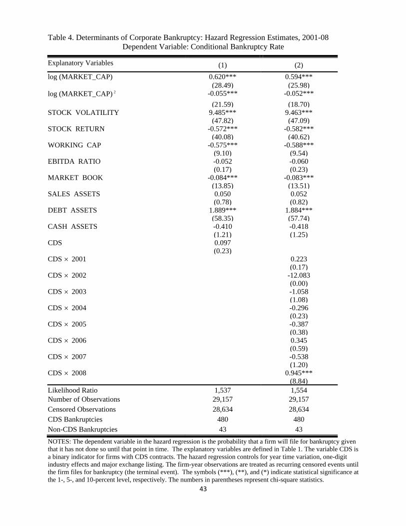
43  

Table 4. Determinants of Corporate Bankruptcy: Hazard Regression Estimates, 2001-08 Dependent Variable: Conditional Bankruptcy Rate

Explanatory Variables (1) (2)

log (MARKET_CAP) 0.620*** 0.594*** (28.49) (25.98)

log (MARKET_CAP) 2 -0.055*** -0.052***

(21.59) (18.70) STOCK VOLATILITY 9.485*** 9.463***

(47.82) (47.09) STOCK RETURN -0.572*** -0.582***

(40.08) (40.62) WORKING CAP -0.575*** -0.588***

(9.10) (9.54) EBITDA RATIO -0.052 -0.060

(0.17) (0.23) MARKET BOOK -0.084*** -0.083***

(13.85) (13.51) SALES ASSETS 0.050 0.052

(0.78) (0.82) DEBT ASSETS 1.889*** 1.884***

(58.35) (57.74) CASH ASSETS -0.410 -0.418

(1.21) (1.25) CDS 0.097

(0.23) CDS 2001 0.223

(0.17) CDS 2002 -12.083

(0.00) CDS 2003 -1.058

(1.08) CDS 2004 -0.296

(0.23) CDS 2005 -0.387

(0.38) CDS 2006 0.345

(0.59) CDS 2007 -0.538

(1.20) CDS 2008 0.945***

(8.84) Likelihood Ratio 1,537 1,554 Number of Observations 29,157 29,157 Censored Observations 28,634 28,634 CDS Bankruptcies 480 480 Non-CDS Bankruptcies 43 43

NOTES: The dependent variable in the hazard regression is the probability that a firm will file for bankruptcy given that it has not done so until that point in time. The explanatory variables are defined in Table 1. The variable CDS is a binary indicator for firms with CDS contracts. The hazard regression controls for year time variation, one-digit industry effects and major exchange listing. The firm-year observations are treated as recurring censored events until the firm files for bankruptcy (the terminal event). The symbols (***), (**), and (*) indicate statistical significance at the 1-, 5-, and 10-percent level, respectively. The numbers in parentheses represent chi-square statistics.

 

44  

Table 5. Impact of CDS on the Probability of Firm Bankruptcy

Pr obabilityCDS Firmgoes bankruptBankruptcyOdds Ratio

Pr obability nonCDS Firmgoes bankrupt

95% Odds Ratio Confidence Limits

Year Bankruptcy Odds Ratio Lower Upper

2001 1.249 0.432 3.612

2002 0.798 0.239 3.084

2003 0.347 0.047 2.557

2004 0.744 0.221 2.508

2005 0.679 0.2 2.311

2006 1.413 0.587 3.401

2007 0.584 0.223 1.53

2008 2.573** 1.38 4.797

NOTES: The odds ratio estimates were derived from the proportional hazard model of bankruptcy presented in the last column of Table 4. A bankruptcy odds ratio equal to 1.5 indicates that the CDS firm has a 50% greater chance of filing for bankruptcy. The symbols (***), (**), and (*) indicate statistical significance at the 1-, 5-, and 10-percent level, respectively.

 

45  

Table 6. The Relationship between Distance to Default and CDS

Dependent Variable: Merton’s DD

Explanatory Variables All Non-Financial Firms Non-Financial Firms

With Bonds (1) (2)

STOCK_VOLATILITY -0.618*** -0.608*** -0.533*** (-12.1) (-12.0) (-9.19)

STOCK RETURN 0.621*** 0.626*** 0.553*** (3.77) (3.81) (3.03)

AGE 0.063 0.062 0.056 (0.88) (0.86) (0.74)

log(MARKET CAP) 0.658*** 0.647*** 0.604*** (6.30) (6.24) (4.89)

WORKING CAP 0.745* 0.802* 0.458 (1.81) (1.96) (0.92)

EBITDA RATIO 0.917*** 0.973*** 0.901** (3.07) (3.26) (2.35)

MARKET BOOK -0.076** -0.064* -0.015 (-2.10) (-1.79) (-0.38)

SALES ASSETS 0.003 0.008 0.046 (0.017) (0.049) (0.20)

DEBT ASSETS -6.44*** -6.47*** -6.29*** (-10.6) (-10.7) (-9.68)

CASH ASSETS 0.910* 0.885* 2.337*** (1.79) (1.75) (3.28)

CDS -0.180 (-0.40)

CDS 2001 0.191 -0.035 (0.22) (-0.041)

CDS 2002 -1.138* -1.151* (-1.74) (-1.78)

CDS 2003 -0.059 -0.019 (-0.10) (-0.033)

CDS 2004 1.031* 0.983* (1.87) (1.82)

CDS 2005 0.850 1.162* (1.40) (1.96)

CDS 2006 0.750 0.989 (1.21) (1.59)

CDS 2007 -0.815 -0.591 (-1.35) (-0.97)

CDS 2008 -2.343*** -2.527*** (-4.64) (-4.94)

Number of Observations 29,011 29,011 20,427 2R 0.74 0.74 0.68

NOTES: The dependent variable is a model-derived Merton’s distance to default. The explanatory variables are defined in Table 1. Models are estimated with robust standard errors. The regression controls for firm fixed effects, yearly time variation, industry effects and major exchange listing. The symbols (***), (**), and (*) indicate statistical significance at the 1-, 5-, and 10-percent level, respectively. The numbers in parentheses represent t statistics.

 

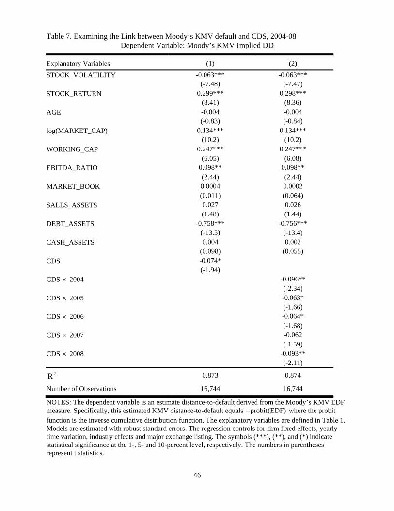
46  

Table 7. Examining the Link between Moody’s KMV default and CDS, 2004-08 Dependent Variable: Moody’s KMV Implied DD

Explanatory Variables (1) (2)

STOCK_VOLATILITY -0.063*** -0.063*** (-7.48) (-7.47)

STOCK_RETURN 0.299*** 0.298*** (8.41) (8.36)

AGE -0.004 -0.004 (-0.83) (-0.84)

log(MARKET_CAP) 0.134*** 0.134*** (10.2) (10.2)

WORKING_CAP 0.247*** 0.247*** (6.05) (6.08)

EBITDA_RATIO 0.098** 0.098** (2.44) (2.44)

MARKET_BOOK 0.0004 0.0002 (0.011) (0.064)

SALES_ASSETS 0.027 0.026 (1.48) (1.44)

DEBT_ASSETS -0.758*** -0.756*** (-13.5) (-13.4)

CASH_ASSETS 0.004 0.002 (0.098) (0.055)

CDS -0.074* (-1.94)

CDS 2004 -0.096** (-2.34)

CDS 2005 -0.063* (-1.66)

CDS 2006 -0.064* (-1.68)

CDS 2007 -0.062 (-1.59)

CDS 2008 -0.093** (-2.11)

2R 0.873 0.874

Number of Observations 16,744 16,744

NOTES: The dependent variable is an estimate distance-to-default derived from the Moody’s KMV EDF measure. Specifically, this estimated KMV distance-to-default equals probit(EDF) where the probit function is the inverse cumulative distribution function. The explanatory variables are defined in Table 1. Models are estimated with robust standard errors. The regression controls for firm fixed effects, yearly time variation, industry effects and major exchange listing. The symbols (***), (**), and (*) indicate statistical significance at the 1-, 5- and 10-percent level, respectively. The numbers in parentheses represent t statistics.

 

47  

Table 8. Regression Analysis Conditional on Bankruptcy: The Impact of CDS before Bankruptcy

Explanatory Variables (1) Merton’s DD (2) Moody’s KMV Implied DD

CONSTANT 4.14** 1.58*** (2.80) (6.32)

STOCK_VOLATILITY -0.546*** -0.098*** (-8.03) (-7.92)

STOCK_RETURN 0.721 0.300 (1.04) (1.89)

AGE -0.053*** -0.004*** (-5.88) (-5.31)

log(MARKET_CAP) 0.359*** 0.128*** (3.71) (8.70)

WORKING_CAP 0.700 0.144* (1.16) (2.66)

EBITDA_RATIO 0.040 0.028 (0.07) (0.51)

MARKET_BOOK 0.063 0.037*** (1.52) (5.66)

SALES_ASSETS 0.016 -0.028 (0.13) (-0.91)

DEBT_ASSETS -2.785*** -1.003*** (-4.80) (-12.43)

CDS Firms Non-CDS Firms F-test CDS Firms Non-CDS Firms F-test BANKRUPTCY -1.493 -1.178*** 0.09 -0.336 -0.285 0.91

(-1.19) (-3.98) (-1.89) (-1.59) BANKRUPTCY-1 -1.010 -1.107*** 0.05 -0.336 -0.159 1.15

(-1.80) (-3.54) (-1.58) (-0.86) BANKRUPTCY-2 -1.393 -0.440 2.3 -0.169 -0.041 6.15*

(-1.78) (-0.91) (-0.92) (-0.21) BANKRUPTCY-3 -1.944** 0.272 4.9 -0.208 -0.152 0.53

(-2.43) (0.55) (-1.07) (-0.70) BANKRUPTCY-4 -1.588*** 0.244 3.46* -0.262 -0.208 2.83

(-3.85) (0.34) (-1.32) (-1.04) BANKRUPTCY-5 -1.716*** 1.040* 64.1***

(-4.13) (1.90) F-test: All Bankruptcy Effects 7.7*** 3.18

Adjusted 2R 0.304 0.612 Observations 1,667 687

NOTES: The variable BANKRUPTCY- (j) is 1 for (j) year before bankruptcy, 0 otherwise; BANKRUPTCY is a binary indicator for year of bankruptcy. All other explanatory variables are defined in Table 1. Models are estimated with robust standard errors. The regression controls for year time variation, one-digit industry effects and major exchange listing. The symbols (***), (**), and (*) indicate statistical significance at the 1-, 5- and 10-percent level, respectively. The numbers in parentheses represent t-statistics. The F-tests investigate the equality of CDS and non-CDS bankruptcy variable coefficients.

 

48  

Table 9. Linear Probability Model for Firms with Existing CDS Contracts

Dependent Variable: A binary indicator for firms with outstanding CDS contracts

Explanatory Variables Parameter Estimates

CONSTANT -0.354*** (-14.46)

DD -0.0017***

(-8.77)

log(ASSETS) 0.074***

(28.35)

log (MARKET_CAP) 0.0185***

(7.23)

AGE 0.0045***

(31.22)

STOCK_RETURN 0.0105**

(2.11)

WORKING_CAP -0.065***

(-8.94)

EBITDA_RATIO -0.090***

(-10.54)

MARKET_BOOK 0.005***

(4.54)

SALES_ASSETS 0.0078***

(3.46)

DEBT_ASSETS 0.048***

(4.68)

CASH_ASSETS 0.057***

(5.06)

ROA -0.038***

(-5.89)

CAPX_ASSETS -0.179***

(-7.11)

GOODWILL -0.045***

(-3.93)

Adjusted 2R 0.53

Number of Observations 29,016

NOTES: The dependent variable in the linear probability model is a binary indicator for firms with existing CDS contracts. Variable definitions: DD=Distance to default; ROA = return-on-assets ratio; CAPX_ASSETS = capital expenditure divided by assets; GOODWILL = goodwill divided by assets. The remaining explanatory variables are defined in Table 1. The linear probability regression includes year dummy controls, one-digit industry effects and major exchange listing indicators. The symbols (***), (**), and (*) indicate statistical significance at the 1-, 5-, and 10-percent level, respectively. The numbers in parentheses represent t statistics.

 

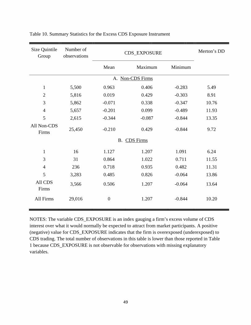
49  

Table 10. Summary Statistics for the Excess CDS Exposure Instrument

Size Quintile Group

Number of observations

CDS_EXPOSURE Merton’s DD

Mean Maximum Minimum

A. Non-CDS Firms

1 5,500 0.963 0.406 -0.283 5.49

2 5,816 0.019 0.429 -0.303 8.91

3 5,862 -0.071 0.338 -0.347 10.76

4 5,657 -0.201 0.099 -0.489 11.93

5 2,615 -0.344 -0.087 -0.844 13.35

All Non-CDS Firms

25,450 -0.210 0.429 -0.844 9.72

B. CDS Firms

1 16 1.127 1.207 1.091 6.24

3 31 0.864 1.022 0.711 11.55

4 236 0.718 0.935 0.482 11.31

5 3,283 0.485 0.826 -0.064 13.86

All CDS Firms

3,566 0.506 1.207 -0.064 13.64

All Firms 29,016 0 1.207 -0.844 10.20

NOTES: The variable CDS_EXPOSURE is an index gauging a firm’s excess volume of CDS interest over what it would normally be expected to attract from market participants. A positive (negative) value for CDS_EXPOSURE indicates that the firm is overexposed (underexposed) to CDS trading. The total number of observations in this table is lower than those reported in Table 1 because CDS_EXPOSURE is not observable for observations with missing explanatory variables.

   

 

50  

 

Table 11. The Relationship between Merton’s Default Risk and Excess CDS Exposure

Explanatory Variables (1) Model Derived DD

(2) Moody’s KMV

Implied DD

STOCK_VOLATILITY -0.569*** -0.061*** (-11.6) (-25.15)

STOCK_RETURN 0.398*** 0.262*** (2.76) (21.65)

AGE 0.110 -0.0001 (1.54) (-0.03)

log(MARKET_CAP) 1.427*** 0.197*** (10.2) (28.41)

WORKING_CAP -0.451 0.120*** (-1.02) (4.85)

EBITDA_RATIO -0.405 -0.010 (-1.21) (-0.46)

MARKET_BOOK -0.060* 0.003 (-1.65) (1.49)

SALES_ASSETS -0.1168 0.011 (-0.63) (1.00)

DEBT_ASSETS -4.620*** -0.585*** (-7.16) (-18.44)

CASH_ASSETS 1.378*** 0.059** (2.74) (2.10)

CDS CDS_EXPOSURE -0.088*** -0.009*** (-6.63) (-15.66)

(1-CDS) CDS_EXPOSURE 0.170*** 0.015*** (9.04) (22.19)

2R 0.75 0.878 Number of Observations 29,011 16,712

NOTES: The dependent variable in Specification (1) is a model-derived distance to default. The dependent variable in Specification (2) is a normalized measure of Moody’s KMV EDFs defined by the

-probit EDF . Specification (2) is only estimated for the period 2004-08. The variable

CDS_EXPOSURE is an index gauging a firm’s excess volume of CDS interest over and above what it would normally be expected to attract from market participants. The explanatory variables are defined in Table 1. Models are estimated with robust standard errors. The regression controls for firm fixed effects, yearly time variation, industry effects and major exchange listing. The symbols (***), (**), and (*) indicate statistical significance at the 1-, 5-, and 10-percent level, respectively. The numbers in parentheses represent t statistics.    

 

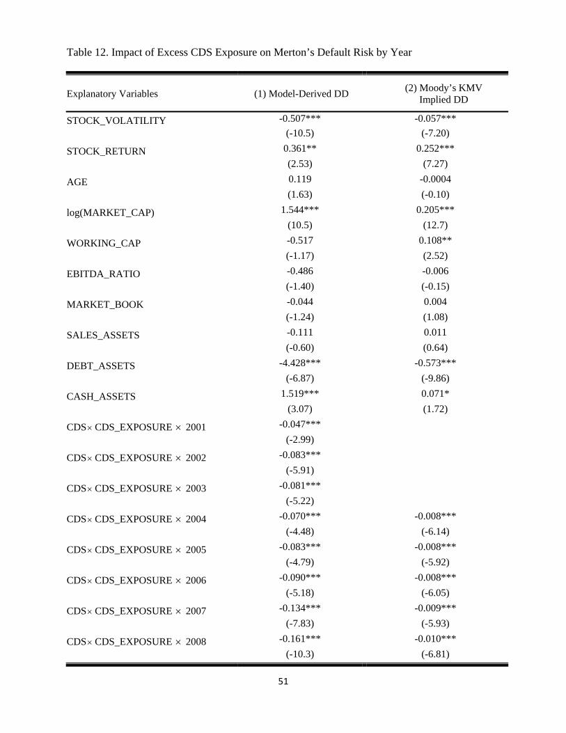
51  

Table 12. Impact of Excess CDS Exposure on Merton’s Default Risk by Year

Explanatory Variables (1) Model-Derived DD (2) Moody’s KMV

Implied DD

STOCK_VOLATILITY -0.507*** -0.057***

(-10.5) (-7.20)

STOCK_RETURN 0.361** 0.252***

(2.53) (7.27)

AGE 0.119 -0.0004

(1.63) (-0.10)

log(MARKET_CAP) 1.544*** 0.205***

(10.5) (12.7)

WORKING_CAP -0.517 0.108**

(-1.17) (2.52)

EBITDA_RATIO -0.486 -0.006

(-1.40) (-0.15)

MARKET_BOOK -0.044 0.004

(-1.24) (1.08)

SALES_ASSETS -0.111 0.011

(-0.60) (0.64)

DEBT_ASSETS -4.428*** -0.573***

(-6.87) (-9.86)

CASH_ASSETS 1.519*** 0.071*

(3.07) (1.72)

CDS CDS_EXPOSURE 2001 -0.047***

(-2.99)

CDS CDS_EXPOSURE 2002 -0.083***

(-5.91)

CDS CDS_EXPOSURE 2003 -0.081***

(-5.22)

CDS CDS_EXPOSURE 2004 -0.070*** -0.008***

(-4.48) (-6.14)

CDS CDS_EXPOSURE 2005 -0.083*** -0.008***

(-4.79) (-5.92)

CDS CDS_EXPOSURE 2006 -0.090*** -0.008***

(-5.18) (-6.05)

CDS CDS_EXPOSURE 2007 -0.134*** -0.009***

(-7.83) (-5.93)

CDS CDS_EXPOSURE 2008 -0.161*** -0.010***

(-10.3) (-6.81)

 

52  

Table 12 continued.

(1-CDS) CDS EXPOSURE 2001 0.180*** (8.57)

(1-CDS) CDS_EXPOSURE 2002 0.211***

(10.2)

(1-CDS) CDS_EXPOSURE 2003 0.159***

(7.49)

(1-CDS) CDS_EXPOSURE 2004 0.145*** 0.015***

(6.77) (6.45)

(1-CDS) CDS_EXPOSURE 2005 0.176*** 0.015***

(6.99) (6.62)

(1-CDS) CDS_EXPOSURE 2006 0.187*** 0.015***

(8.39) (6.76)

(1-CDS) CDS_EXPOSURE 2007 0.232*** 0.016***

(9.16) (7.06)

(1-CDS) CDS_EXPOSURE 2008 0.254*** 0.018***

(12.2) (7.93)

2R 0.751 0.879

Number of Observations 29,011 16,712***

NOTES: The dependent variable in Specification (1) is a model-derived distance to default. The dependent variable in Specification (2) is a normalized measure of Moody’s KMV EDFs defined by the

-probit EDF . Specification (2) is only estimated for the period 2004-08. The variable

CDS_EXPOSURE is an index gauging a firm’s excess volume of CDS interest over and above what it would normally be expected to attract from market participants. The explanatory variables are defined in Table 1. Models are estimated with robust standard errors. The regression controls for firm fixed effects, yearly time variation, industry effects and major exchange listing. The symbols (***), (**), and (*) indicate statistical significance at the 1-, 5-, and 10-percent level, respectively. The numbers in parentheses represent t statistics.

 

53  

Table 13. Investigating the Impact of Financial Fragility on Corporate Default

Dependent Variable = Implied Distance to Default

Explanatory Variables

(1) Model-Derived DD (2) Moody’s KMV Implied DD

STOCK_VOLATILITY -0.552*** -0.063*** (-11.3) (-8.12)

STOCK_RETURN 0.507*** 0.312*** (3.65) (13.7)

AGE 0.126* -0.002 (1.74) (-0.41)

log(MARKET_CAP) 1.208*** 0.195*** (8.98) (13.5)

WORKING_CAP 0.202 0.159*** (0.45) (4.03)

EBITDA_RATIO 0.004 -0.027 (0.014) (-0.75)

MARKET_BOOK -0.067* 0.0002 (-1.79) (0.076)

SALES_ASSETS -0.122 0.018 (-0.63) (1.07)

DEBT_ASSETS -4.894*** -0.536*** (-7.11) (-9.53)

CASH_ASSETS 1.216** 0.034 (2.46) (0.87)

CDS Controls

CDS CDS_EXPOSURE -0.053*** -0.008*** (-4.07) (-6.31)

(1-CDS) CDS_EXPOSURE 0.116*** 0.014*** (6.24) (7.35)

Table 13 continued next page

 

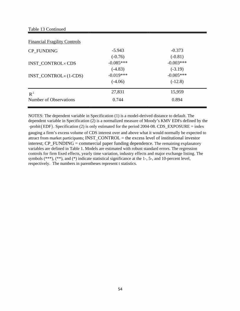
54  

NOTES: The dependent variable in Specification (1) is a model-derived distance to default. The dependent variable in Specification (2) is a normalized measure of Moody’s KMV EDFs defined by the

-probit EDF . Specification (2) is only estimated for the period 2004-08. CDS_EXPOSURE = index

gauging a firm’s excess volume of CDS interest over and above what it would normally be expected to attract from market participants; INST_CONTROL = the excess level of institutional investor interest; CP_FUNDING = commercial paper funding dependence. The remaining explanatory variables are defined in Table 1. Models are estimated with robust standard errors. The regression controls for firm fixed effects, yearly time variation, industry effects and major exchange listing. The symbols (***), (**), and (*) indicate statistical significance at the 1-, 5-, and 10-percent level, respectively. The numbers in parentheses represent t statistics.

Table 13 Continued

Financial Fragility Controls

CP_FUNDING -5.943 -0.373 (-0.76) (-0.81)

INST_CONTROLCDS -0.085*** -0.003*** (-4.83) (-3.19)

INST_CONTROL (1-CDS) -0.019*** -0.005*** (-4.06) (-12.8)

2R 27,831 15,959

Number of Observations 0.744 0.894

%

150%

200%

250%

300%

30

40

50

60

70

80

% International Total Debt

Figure 1. Growth of CDS Market, 2001-09Gross Notional CDS ($ trillions) 

0%

50%

100%

0

10

20

2000 2001 2002 2003 2004 2005 2006 2007 2008 2009

CDS Gross Notional %International DebtSources: Markit and ISDA

40

50

60

70

80

90

100

Figure 2. Fraction of CDS Firms by Asset Percentiles

% CDS Firms

0

10

20

30

0 10 20 30 40 50 60 70 80 90 100

Asset Percentiles

Source: Markit and Compustat

0

0.02

0.04

0.06

0.08

0.1

‐7 0 4 8 13 17 22 26 31

Distance to Default

Density

Figure 3. Kernel Density Estimate of Distance to Default and Implied Default Probability

Density

0

0.05

0.1

0.15

0.2

0.25

0.000 0.025 0.050 0.075 0.100

Implied Default Probability

CDS Firms Non‐CDS Firms

0

4

8

12

16

20

2001 2002 2003 2004 2005 2006 2007 2008

Figure 4. Default Risk for CDS and Non-CDSFirms by Year, 2001-08

A. Distance to Default

B Implied Default Probability

0

0.02

0.04

0.06

0.08

2001 2002 2003 2004 2005 2006 2007 2008

Non‐CDS Firms CDS Firms

B. Implied Default Probability

0

0.02

0.04

0.06

0.08

0.1

0.12

‐7 0 3 6 8 11 13 15 17 19 21 24

Density

Figure 5. Kernel Density Estimate of Distance to DefaultOver Time

Distance to Default

A.CDS Firms

Density B. Non‐CDS Firms

0

0.02

0.04

0.06

0.08

0.1

0.12

‐7 ‐1 3 7 11 16 20 24

2001‐2006 2008

Density B. Non CDS Firms

Distance to Default

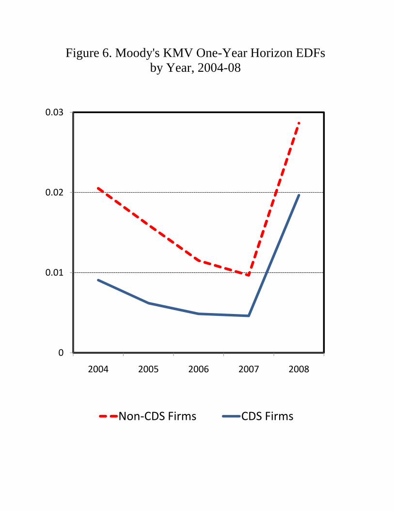
0 01

0.02

0.03

Figure 6. Moody's KMV One-Year Horizon EDFsby Year, 2004-08

0

0.01

2004 2005 2006 2007 2008

Non‐CDS Firms CDS Firms

0

0.05

0.1

0.15

0.2

0.25

0.000 0.018 0.035 0.053 0.070

EDFs

Density

Figure 7. Kernel Density Estimate of Moody'sKMV EDFs, 2004-08

0 12Density

0

0.02

0.04

0.06

0.08

0.1

0.12

0.4 0.7 1.1 1.4 1.7 2.1 2.4 2.7 3.1 3.4 3.7

Implied Distance to Default

CDS Firms Non‐CDS Firms

4

6

8

Gross Notional Ratio

Figure 8. The Relationship between Excess CDS Exposure in 2008 and the Gross Notional Ratio in 2009

0

2

0 0.2 0.4 0.6 0.8 1

Excess CDS Exposure

Source: DTCC and authors' calculations