are business cycles all alike?
TRANSCRIPT


128 Olivier J. Blanchard/Mark W. Watson
Reduced-Form Estimation
Since we impose no restrictions on the lag structure, A;, i = 1, ... ,n,we can proceed in two steps. The reduced form associated with equa-tion (1) is given by:
(2)n
Xt = 2: B;Xt-; + Xt;=1
E(x,x~) = n= 0
if t = T
if t =1= T
B; = (I - AO)-lA; ; n = [(I - Ao)-l]D[(I - AO)-l]'.
We first estimate the unconstrained reduced form (2). Under the large-shock hypothesis, some of the realizations of the E t and thus X t maybe large; we therefore use a method of estimation that may be moreefficient than ordinary least squares (OLS) in this case. We use thebounded influence method developed by Krasker and Welsch (1982),which in effect decreases the weight given to observations with largerealizations. 5 We choose a lag length, n, equal to 4.6
The vector X t is the vector of unexpected movements in Y, P, M, andG. Let lower-case letters denote unexpected movements in these vari-ables, so that this first step in estimation gives us estimated time seriesfor y, p, m, and g.
Structural Estimation
The second step takes us from x to E. Note that equations (1) and(2) imply:
(3) x = Ao x + E.
Thus, to go from x to E we need to specify and estimate Ao, the setof contemporaneous relations between the variables. We specify thefollowing set of relations:
(4) Y bIP + ES (aggregate supply)
(5) Y b2m b3P + b4g + Ed (aggregate demand)
(6) g C1Y + C2P + Eg (fiscal rule)
(7) m C3Y + C4P + Em (money rule)
5. LAD or other robust M estimators could also have been used. In some circum-stances OLS may be more efficient than the robust estimators because of the presenceof lagged values.
6. Each equation in the vector autoregression included a constant and a linear timetrend. When the vector autoregression was estimated without a time trend, the esti-mated residuals, x, were essentially unchanged.

129 Are Business Cycles All Alike?
We have chosen standard specifications for aggregate supply anddemand. Output supplied is a function of the price level.? Output de-manded is a function of nominal money, the price level, and fiscalpolicy; this should be viewed as the reduced form of an IS-LM model,so that Cd is a linear combination of the IS and LM disturbances. Thelast two equations are policy rules, which allow the fiscal index andmoney to respond contemporaneously to output and the price level. 8
Even with the zero restrictions on Ao implicit in the equations above,the system of equations (4) to (7) is not identified. The model containseight coefficients and four variances that rnust be estimated from theten unique elements in O. To achieve identification, we use a prioriinformation on two of the parameters.
Within a quarter, there is little or no discretionary response of fiscalpolicy to changes in prices and output. Most of the response dependson institutional arrangements, such as the structure of income tax rates,the degree and timing of indexation of transfer payments, and so on.Thus the coefficients Ct and C2 can be constructed directly; the detailsof the computations are given in appendix 2.2. Using these coefficients,we obtain f! from equation (6).
Given the two constructed coefficients CI and C2, we now have sixunknown coefficients and four variances to t~stimate using the ten uniqueelements in O. The model is just identifit~d. Estimation proceeds asfollows: Eg is used as an instrument in equation (4) to obtain ES
; ~ andES are used as instruments in equation (7) to obtain Em. Finally, Eg, ES ,
and Em are used as instruments in equation (5) to obtain Ed'The validity of these instruments at each stage depends on the plau-
sibility of the assumption that the relevant disturbances are not cor-related. Although we do not believe this is exactly the case, we find itplausible that they have a low correlation, so that our identification isapproximately correct.
It may be useful to compare our method for identifying and estimatingshocks with the more common method used in the vector autoregres-
7. A more detailed specification of aggregate supply, recognizing the effects of theprice of materials would be:
y = dIP - d 2(Pm -p)
Pm = d3P + d4y+ eYS
+ epm ,
where supply depends on the price of materials, Pm' and the price level, and where intum the nominal price of materials depends on the price level and the level of output.The two equations have, however, the same specifica.tion, and it is therefore impossibleto identify separately the shocks to the price of materials and to supply epm and eYS •
Equation (4) is therefore the solved-out version of this two-equation system, and eS isa linear combination of these two shocks.
8. If money supply responds to interest rates directly rather than to output andprices, em and ed will both depend partly on money demand shocks and thus will becorrelated. Our estimation method will then attribute as much of the variance as pos-sible to em and incorporate the residual in Ed.

130 Olivier J. Blanchard/Mark W. Watson
sion literature. A common practice in that literature is to decompose,as we do, the forecast errors into a set of uncorrelated shocks. Therethe identification problem is solved by assuming that the matrix (I Ao) is triangular or can be made triangular by rearranging its rows. Thisyields a recursive structure that is efficiently estimated by OLS. Wedo not assume a recursive structure but rather impose four zero re-strictions in addition to constructing two coefficients Ct and Cz. Ourmethod produces estimated disturbances much closer to true structuraldisturbances than would be obtained by imposing a recursive structureon the model.
2.3 The Direct Approach: Results
2.3.1 Reduced-Form EvidenceThe first step is the estimation of the reduced form given by equation
(2). The estimated Bj, i = 1, ... , 4 are of no particular interest. Theestimated time series corresponding to unexpected movements of xthat is of y, m, p, and g-are of more interest. Table 2.1 gives, for y,m, p, and g, the value of residuals larger than 1.5 standard deviationsin absolute value, as well as the associated standard deviation andestimated kurtosis.
The kurtosis coefficient of a normally distributed random variable isequal to 3. The 99% significance level of the kurtosis coefficient, for asample of 120 observations drawn from a normal distribution, is 4.34.Thus, ignoring the fact that these are estimated residuals rather thanactual realizations, three of the four disturbances have significantly fattails. Since linear combinations of independent random variables havekurtosis smaller than the maximum kurtosis of the variables them-selves, this strongly suggests large kurtosis of the structural disturb-ances. 9 We now turn to structural estimation.
2.3.2 The Structural CoefficientsThe second step is estimation of Ao, from equations (4) to (7). We
use constructed values for Ct and Cz of - 0.34 and - 1.1 respectively.Unexpected increases in output increase taxes more than expendituresand lead to fiscal contraction. Unexpected inflation increases real taxesbut decreases real expenditures, leading also to fiscal contraction. Weare less confident of cz, the effect of inflation, than we are of Ct. In
9. A more precise statement is the following: Let Xl and X 2 be independent variableswith kurtosis K I and K 2 , one of which is greater than or equal to 3. Then if Z is a linearcombination of Xl and X 2 , K z ~ max (K.,K2 ). We do not, however, assume indepen-dence but only assume zero correlation of the structural disturbances.

131 Are Business Cycles All Alike?
Table 2.1 Large Reduced-Form DisturbancE~s
Date y g m p
1948:4 -2.61949:1 -2.21949:4 -2.41950:1 3.2 2.61950:2 -5.1 1.61950:3 1.8 -1.6 5.11951: 1 3.71951:2 4.2 -2.81951:3 2.2 -1.61951:4 1.61952:2 1.61952:3 1.71952:4 1.61953:1 1.61953:4 -1.61954:1 -1.7 2.11958: 1 -2.21959:1 -1.81959:3 -2.71959:4 -2.91960:1 2.2 -2.71960:4 -1.91962:3 -1.51965:4 1.61966:3 -2.21967:3 1.81970:4 -1.81971 :3 -1.61972:2 -1.51972:4 1.71974:4 -1.6 1.71975:1 -3.11975:2 3.6 -1.71975:3 -3.11975:4 -1.61978:2 2.2 2.11979:2 1.71980:2 -2.5 -4.21980:3 2.4 4.71981:3 -3.51982:4 3.0Standard error .0085 .0431 .0244 .0182Kurtosis 4.0 10.2 8.6 8.2
Note: Ratios of residuals to standard errors are reported.

132 Olivier J. Blanchard/Mark W. Watson
appendix 2.1 we report alternative structural coefficient estimates basedon C2 = -1.3 and C2 = -1.0.
The results of estimating equations (4) to (7) are reported in table2.2. All coefficients except one are of the expected sign. Nominal moneyhas a negative contemporaneous effect on output; this is consistentwith a positive correlation between unexpected movements in moneyand output because of the positive effect of output on money supply.Indeed the correlation m and y is .32. (Anticipating results below, wefind that the effect of nominal money on output is positive after onequarter.) Aggregate supply is upward sloping; a comparison with theresults of table 2.A.1 suggests that the slope of aggregate supply issensitive to the value of C2.
Given our estimates of the reduced form and of Ao, we can nowdecompose each variable (Y, P, M, G) as the sum of four distributedlags of each of the structural disturbances ed, eS
, em, and eg • Technically,we can compute the structural moving average representation of thesystem characterized by equation (1).
2.3.3 One or Many Sources of Shocks? Variance DecompositionDoes one source of shocks dominate? We have seen that a natural
way of answering this question is to characterize the contribution ofeach disturbance to the unexpected movement in each variable. Wedefine unexpected movement as the difference between the actual valueof a variable and the forecast constructed K periods earlier using equa-tion (1). We use three values ofK. The first case, K = 1, decomposesthe variance ofy, p, m, and g into their four components, the variancesofed, eS , em and eg • The other two values, K = 4 and K = 20, correspondto the medium run and the long run respectively.
The results are reported in table 2.3. Demand shocks dominate outputin the short run; supply shocks dominate price in the short run. In the
Table 2.2 Structural Estimates
Fiscala
Money supply
Aggregate supply
Aggregate demand
Standard deviations
g = -.34y - 1.1pm = 1.40y + .19p
(1.4)b (.7)
y = .81p(1.1)
y = - .10p - .20m + .06g( - 3.1) ( - 2.2) (2.4)
.041 .024 .017Ed
.011
acoefficients constructed, not estimated.bt-statistics in parentheses.

133 Are Business Cycles All Alike?
Table 2.3 Variance Decompositions
Structural Disturbance
Eg ES Em Ed
ContemporaneouslyY - E_1Y .03 .19 .04 .74G - E_1G .78 .14 .00 .08M - E_1M .01 .01 .74 .25P - E_1P .01 .74 .01 .24Four quarters aheadY - E_4 Y .15 .16 .16 .54G - E_ 4G .70 .13 .00 .16M - E_ 4M .13 .03 .67 .17P - E_ 4P .01 .6.5 .01 .33
Twenty quarters aheadY - E_ 20 Y .27 .20 .17 .37G - E_ 20G .66 .12 .05 .17M - E_ 20M .28 .04 .64 .05P - E_ 20P .15 .22 .36 .26
medium and long run, however, all four shocks are important in explaining the behavior of output and prices. There is no evidence insupport of the one dominant source of shocks theory.
2.3.4 Are There Infrequent Large Shocks? ITable 2.4 reports values and dates for all estimated realizations of
ed,es ,em and eg larger than 1.5 times their respective standard deviation.We can compare these with traditional, informal accounts of the historyof economic fluctuations since 1948 and see whether specific eventsthat have been emphasized there correspond to large realizations. Auseful, concise summary of the events associated with large postwarfluctuations is contained in table 1.1 in the paper by Eckstein and Sinaiin this volume (chap. 1).
The first major expansion in our sample, from 1949:4 to 1953:2, isusually explained both by fiscal shocks associated with the Korean Warand by a sharp increase in private spending. We find evidence of bothin 1951 and in 1952. From 1955 to the early 1970s, large shocks arefew and not easily interpretable. There are, for example, no large shocksto either fiscal policy or private spending corresponding to either theKennedy tax cut or the Vietnam War. In the 1970s, major fluctuationsare usually explained by the two oil shocks. There is some evidencein favor of this description. We find two large supply shocks in 1974:4and 1975: 1; we also find large fiscal and large demand shocks during

134 Olivier J. Blanchard/Mark W. Watson
Table 2.4 Large Structural Disturbances
Date Fiscal Supply Money Demand
1948:3 1.91948:4 2.51949:1 -1.5 -1.91949:4 -1.81950: 1 3.0 1.8 2.01950:2 -4.6 -1.61950:3 -3.7 3.61951: 1 1.7 -3.61951:2 3.1 3.21951:3 1.6 1.81951:4 1.61952:2 1.51952:3 2.01952:4 1.71953:4 -1.61954:1 -2.81954:3 1.81957:4 -1.71958:1 -1.5 -1.71958:3 1.71959: 1 -1.61959:3 -2.31959:4 -2.61960: 1 -2.6 2.41960:3 1.51960:4 -2.01966:3 -2.21968:4 1.51971 :2 2.11971 :3 -1.81972:2 1.61972:4 1.71974:4 -2.41975: 1 -2.5 -2.41975:2 3.1 1.91975:3 -3.11975:4 -1.81978:2 2.71979:2 1.61980:2 -2.1 -3.2 -2.71980:3 3.4 3.41981 :2 1.61981 :3 -3.81982: 1 1.61982:4 3.7

135 Are Business Cycles All Alike?
the same period. The two recessions of the early 1980s are usuallyascribed to monetary policy. We find substantial evidence in favor ofthis description. There are large shocks to money supply for most ofthe period 1979:2 to 1982:4 and two very large negative shocks in 1980:2and 1981:3.
The overall impression is therefore one of infrequent large shocks,but not so large as to dominate all others and the behavior of aggregatevariables for long periods. To confirm this impression, we report thekurtosis coefficients of the structural disturbances in table 2.5A; in allcases we can reject normality with high confidence. In table 2.5B weuse another descriptive device. We assunle that each structural dis-turbance is an independent draw from a mixed normal distribution, thatis for x = g, d, s, or m:
with probability 1 - Px
with probability Px
where
The realization of each disturbance is drawn either from a normaldistribution with large variance, with probability P, or from a normaldistribution with small variance, with probability 1 - P. The estimatedvalues of (Jlx' (J2x, Px , estimated by maximum likelihood, are reportedin table 2.5B. The results suggest large, but not very large, ratios ofthe standard deviation of large to the standard deviation of small shocks;they also suggest infrequent, but not very infrequent, large shocks.The estimated probabilities imply that one out of six fiscal or moneyshocks and one out of three supply or deInand shocks carne from thelarge variance distributions.
Table 2.5 Characteristics of Structural Disturbances
A. Estimated kurtosis Eg E S Em Ed
K 7.0 5.4 5.9 4.6B. Disturbances as mixed normals
0'1 .68 .63 .72 .68(.08)a (.10) (.09) (.13)
0'2 2.01 1.62 1.97 1.50(.64) (.41) (1.03) (.41)
Ratio 2.95 2.57 2.73 2.21Probability .15 .27 .14 .30
(.09) (.15) (.15) (.22)
aStandard errors in parentheses.

136 Olivier J. Blanchard/Mark W. Watson
The dating of the large shocks in table 2.4 suggests two more char-acteristics of shocks. First, large shocks tend to be followed by largeshocks, suggesting some form of autoregressive conditional hetero-skedasticity as discussed in Engle (1982). Second, there seems to besome tendency for large shocks to happen in unison. In 1950: 1, forexample, we find large fiscal, supply, and demand shocks, whereas in1980:3 we find large supply, money, and demand shocks. To confirmthese impressions we present in table 2.6 the correlations and firstautocorrelations between the squares of the structural shocks. 10 Thetable shows a large positive contemporaneous correlation between thesquare of the supply shock and the square of the demand shock. Aweaker contemporaneous relationship between supply and the fiscalshock is present. The squares of all shocks are positively correlatedwith their own lagged values; there is also significant correlation be-tween demand, the lagged fiscal and supply shocks, and the fiscal shockand lagged supply shock. All in all, these results suggest an economycharacterized by active, volatile periods followed by quiet, calm pe-riods, both of varied duration.
2.3.5 Are There Infrequent Large Shocks? IIWe discussed in section 2.2 the possibility that a specific source of
shocks may dominate some episode of economic fluctuations, even ifthere are no large realizations of the shock. To explore this possibility,we construct an unexpected output series, where the expectations arethe forecasts of output based on the estimated model corresponding toequation (1), eight quarters before. We chose eight quarters becausethe troughs and peaks in this unexpected output series correspondclosely to NBER troughs and peaks. We then decompose this forecast
Table 2.6 Correlations between Squares of Structural Disturbances
(eg)2 (es)2 (e ffi)2 (ed)2
(eg )2 .27 - .05 .08(es )2 -.01 .36(em )2 .28(ed)2
(e~J)2 .33 .43 .00 .33
(e~J)2 .35 .38 .03 .13
(e'!!J)2 .02 -.09 .23 .21
(e~J)2 .15 .08 .13 .16
10. Although the contemporaneous correlation between the levels of the shock is zeroby construction, the same is not true of the squares of the shocks.

137 Are Business Cycles All Alike?
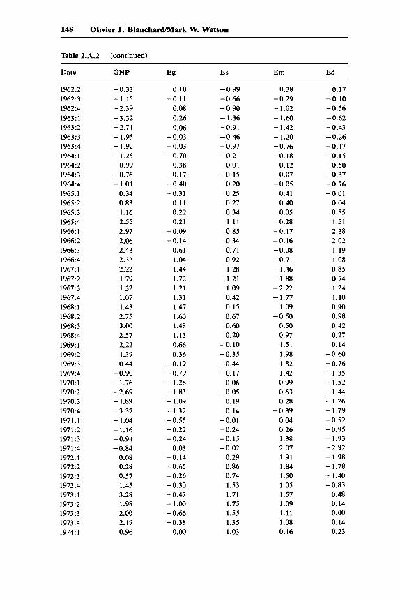
error for GNP into components due to each of the four structuraldisturbances. This decomposition is repres1ented graphically in figure2.1; the corresponding time series are given in table 2.A.2 in appendix2.1.
No single recession can be attributed to only one source of shock.Post-war recessions appear to be due to the combination of two orthree shocks. The 1960:4 trough, for example, where the GNP forecasterror is - 6.7%, is attributed to a fiscal shock component (- 2.4%), asupply shock component (-1.1%), a money shock component (-1.7%),and a demand shock component (-1.4%). The 1975:1 trough, wherethe GNP forecast error is also -6.7%, seems to have a large supplyshock component (-3.6%) and a demand shock component (-2.9%).The 1982:4 trough, where the GNP forecast error is - 4.5%, is decom-posed as -1.4% (fiscal), 1.1% (supply), -1.4% (money), and -2.8%(demand).
To summarize the results of this section, \\i'e find substantial evidenceagainst the single source of shock hypothesis. We find some evidenceof large infrequent shocks; however, they do not seem to dominateeconomic fluctuations.
2.4 The Indirect Approach
If economic fluctuations are due to an accumulation of small shocks,then in some sense business cycles should all be alike. In this sectionwe make precise the sense in which cycles should be alike and examinethe empirical evidence.
The most influential contribution to the position that cycles are alikeis the empirical work carried out by Burns and Mitchell (1946) on pre-World War II data. Their work focused not only on the characteristiccyclical behavior of many economic variables but also on how, in spe-cific cycles, the behavior of these variables differed from their char-acteristic cyclical behavior. Looking at their graphs, one is impressedat how similar the behavior of most variables is across different cycles;this is true not only of quantities, for which it may not be too surprising,but also, for example, of interest rates.
We considered extending the Burns/Mitchell graph method to theeight postwar cycles but decided against it. l\1any steps of the method,and in particular their time deformation, are judgmental rather thanmechanical. As a result, it is impossible to derive the statistical prop-erties of their results. When comparing the graphs of short rates acrosstwo cycles, for example, we have no statistical yardstick to decidewhether they are similar or significantly different. As a result also, wedo not know which details, in the wealth of details provided in thesegraphs, should be thought of as significant.

PT
rA:
PERC
ENTA
GEP
OIN
TS
2.5
~;J
IAJlIII
.I11Irvi:
':'1AII
IIIft
llllll
il11111:
Pe
rce
nt
GNP
0.0
Va
ria
nce
-2.5
rrr
ImyIV
yr'T
Ilililll!
lill1111
lill1
00
f\~~I
ijl~ij~:~
:~2.
5DE
MAND
0.0
I-
Vf~
~I
ltV\1~
-~/
I~IN
rI:~
:Irt~~1
38-2
.5 2.5
MON
EYo.
Or~
IJV
'iiV
IV\.
/\J
I~trII~J~
19
-2.5
.....
-a-a-
-.....
.
2.5
SU
PP
LY0.
0L
f\~~
ImL
~~m~W~II
18
-2.5 2.5
FIS
CA
L0
.0L
,,/'
II~J
\IIJ~[I~~~t~l
~-.~~]
25-2
.5
4850
5254
5658
6062
6466
6870
7274
7678
8082
YEAR
Fig.
2.1
Com
pone
nts
ofG
NP
fore
cast
erro
r.

139 Are Business Cycles All Alike?
Therefore we use an approach that is in the spirit of Burns andMitchell but allows us to derive the statistical properties of the esti-mators we use. The trade-off is that the statistics we give are muchless revealing than the Burns/Mitchell graphs. Our approach is to com-pute the cross-correlations at different leads and lags between variousvariables and a reference variable such as G~~P, across different cycles.
2.4.1 The Construction of Correlation CoefficientsThe first step is to divide the sample into subsamples. We adopt the
standard division into cycles, with trough points determined by theNBER chronology. This division may not be, under the large-shockhypothesis, the most appropriate, since a large shock may well dom-inate parts of two cycles. It is, however, the least controversial. De-fining the trough-to-trough period as a cycle.t there are seven completecycles for which we have data; their dates are given in table 2.7. Thisgives us seven subsamples.
For each subsample, we compute cross-correlations at various leadsand lags between the reference variable and the variable considered.Deterministic seasonality is removed from all variables before the cal-culation of the correlations. A more difficult issue is that of the timetrend: the series may be generated either by a deterministic time trendor by a stochastic time trend or by both. In the previous two sections,this issue was unimportant in the sense that inclusion or exclusion ofa deterministic trend together with unconstrained lag structures in thereduced form made little difference to estimated realizations of thedisturbances. Here the issue is much more important. Computing de-viations from a single deterministic trend for the whole sample may bevery misleading if the trend is stochastic. ()n the other hand, takingfirst or second differences of the time series probably removes non-stationarities associated with a stochastic trend, but correlations be-tween first or second differences of the time series are difficult tointerpret.
In their work, Burns and Mitchell adopt an agnostic and flexiblesolution to that problem: they compute deviations of the variables fromsubsample means. Thus they proxy the time trend by a step function.Although this does not capture the time trend within each subsample,it does imply that across subsamples, the estimated time trend willtrack the underlying one. We initially follo\\'ed Burns and Mitchell intheir formalization but found this procedure to be misleading for vari-ables with strong time trends. During each subsample, both the ref-erence and the other variable are below their means at the beginningand above their means at the end; this generates spuriously high cor-relation between the variables. We modify the Burns/Mitchell proce-dure as follows: for each subsample, we allow for both a level and a

140 Olivier J. Blanchard/Mark W. Watson
time trend; the time trend is given by the slope of the line going fromtrough to trough. This should be thought of as a flexible (perhaps tooflexible) parameterization of the time trend, allowing for six level andslope changes over the complete sample.
The cross-correlations are then computed for deviations of each ofthe two series from its trend. We compute correlations of the referencevariable and of the other variable, up to two leads and lags.
2.4.2 The Construction of Confidence LevelsFor each variable we calculate cross-correlations with our reference
variable, GNP, for each of the seven cycles. We then want to answerthe following questions: Should we be surprised by the differences inestimated correlation across cycles? More precisely, under the nullhypothesis that fluctuations are due to the accumulation of small shocks,how large are these differences in the correlation coefficients likely tobe? Thus, we must derive the distribution of the differences betweenthe largest and smallest correlation coefficients, at each lag or lead foreach variable. This distribution is far too difficult to derive analytically;instead we rely on Monte Carlo simulations.
The first step is to estimate, for each variable, the bivariate processgenerating the reference variable and the variable under consideration.We allow for four lags of each variable and a linear time trend, for theperiod 1947: 1 to 1982:4. The method of estimation is, for the samereasons as in section 2.2, Krasker-Welsch.
The second step is to simulate the bivariate process, using disturb-ances drawn from a normal distribution for disturbances. (Thus weimplicitly characterize the "small-shock" hypothesis as a hypothesisthat this joint distribution is normal.) We generate 1,000 samples of 147observations each. We then divide each sample into cycles by identi-fying troughs in the GNP series. Let X t denote the log of real GNP attime t. Time t is a trough if two conditions are satisfied. The first isthat Xt-l > X t < Xt+l < X t +2 < X t +3, and the second that X t be at least0.5 % below the previous peak value of x. The first ensures that ex-pansions are longer than three periods, and the second eliminates minordownturns. (When applied to the actual sample, this rule correctlyidentifies NBER troughs, except for two that differ from the NBERtrough by one quarter.) Given this division into cycles, we compute,as in the actual sample, cycle-specific correlations and obtain, for eachof the 1,000 samples, the difference between the largest and the smallestcorrelation. Finally, by looking at the 1,000 samples, we get an empiricaldistribution for the differences.
What we report in table 2.7 for each variable and for correlations ateach lead and lag are probabilities that in the corresponding empiricaldistributions the difference between the largest and smallest correlation

141 Are Business Cycles All Alike?
exceeds the value of this difference in the actual sample. This proba-bility is denoted p. A very small value ofp indicates that the differenceobserved in the actual sample is surprisingly large under the smallshock hypothesis. It would therefore be e:vidence against the small-shock hypothesis.
2.4.3 The Choice of VariablesMost quantity variables, such as consumption or investment, ap-
pear highly correlated with real GNP. Most of the models we haveimply that it should be so, nearly irrespective of the source of shocks.Most models imply that correlations of prices and interest rates withGNP will be of different signs depending on the source of shocks.We report results for various prices, inter,est rates, policy variables,and quantities.
We look at three real wages. In all three cases, the numerator is thesame, the index of average hourly earnings of production and nonsu-pervisory workers, adjusted for overtime and interindustry shifts, inmanufacturing. In table 2.7A, the wage is dt~flated by the GNP deflator.In table 2.7B, it is deflated by the CPI and is therefore a consumptionreal wage. In table 2.7C, it is deflated by the producer price index formanufacturers and is therefore a product ~'age. In all three cases, wetake the logarithm of the real wage so constructed.
We then look at two relative prices. Both are relative prices of ma-terials in terms of finished goods. Because of the two oil shocks, weconsider two different prices. The first is thle ratio of the price of crudefuel to the producer price index for finisht~d goods and is studied intable 2.7D. Table 2.7E gives the behavior of the price of nonfood,nonfuel materials in terms of finished goods.
We then look at the behavior of interest rates. Table 2.7F charac-terizes the behavior of the nominal three month treasury bill rate. Table2.7G gives the behavior of Moody's AAA corporate bond yield.
We consider the two policy variables: the fiscal index defined inthe first section, and nominal MI' The results are given in tables 2.7Hand I.
Finally, we consider three quantity variables. Table 2.7J shows thebehavior of real consumption expenditures. Table 2.7K and L showsthe behavior of nonresidential and residential investment.
2.4.4 General ResultsIn looking at table 2.7, there are two types of questions we want
to answer. The first is not directly the subject of the paper but isclearly of interest. It is about the typical behavior of each variablein the cycle. The answer is given for each variable by the sequenceof average correlation coefficients at the different lags and leads.

142 Olivier J. Blanchard/Mark W. Watson
Table 2.7 Correlations
Cycle Trough to Trough Peak1 1949:4 to 1954:2 1953:22 1954:2 to 1958:2 1957:33 1958:2 to 1961: 1 1960:24 1961:1 to 1970:4 1969:45 1970:4 to 1975: 1 1973:46 1975: 1 to 1980:2 1979:47 1980:2 to 1982:4 1981:2Pi = correlation between tpe reference variable, logarithm of real GNP at time t, andthe other variable at time t + i.
Real Wages
A. Real wage in terms of the GNP deflator (in log)Cycle P-2 P-l Po P+l P+21 - .81 -.70 -.36 -.25 .092 -.06 -.41 -.48 - .18 .443 - .17 .02 .03 -.35 -.594 - .11 - .13 -.01 -.04 -.005 .85 .90 .90 .65 .376 .75 .84 .84 .75 .637 .62 .61 .06 -.29 - .38Average - .15 -.16 .14 .04 .08Difference 1.67 1.61 1.38 1.10 1.22p .04 .07 .27 .65 .52B. Real wage in terms of the CPI (in log)Cycle P-2 P-l Po P+l P+21 -.53 - .58 - .57 -.64 -.572 .09 .44 .79 .85 .763 -.15 .29 .75 .47 -.074 .56 .57 .63 .56 .495 .84 .67 .47 .02 - .316 .78 .89 .88 .78 .657 .57 .32 -.31 -.53 -.24Average .30 .37 .37 .21 .10Difference 1.37 1.47 1.45 1.49 1.34p .48 .31 .32 .22 .49C. Real wage in terms of the PPI (in log)Cycle P-2 P-l Po P+l P+21 -.68 - .71 -.63 -.55 -.282 .17 .60 .91 .88 .633 -.29 .45 .87 .62 .274 -.46 -.56 -.62 -.72 -.765 .88 .74 .52 .08 - .276 .78 .86 .82 .71 .597 -.42 -.70 -.72 -.60 .01Average -.02 .09 .16 .06 .02Difference 1.57 1.57 1.62 1.61 1.40p .17 .18 .13 .11 .44

143 Are Business Cycles All Alike?
liIble 2.7 (continued)
Relative Prices
D. Relative price of crude fuels in terms of finished goods (in log)Cycle P-2 P-l Po P+l P+21 -.65 -.61 -.45 -.43 -.192 -.25 -.04 .09 .31 .413 -.07 .45 .42 .46 .174 -.61 -.75 -.86 -.91 -.915 -.66 -.86 - .91 -.81 -.636 .47 .46 .35 .34 .447 -.56 -.39 -.23 -.16 -.01Average -.33 -.24 -.22 -.17 -.10Difference 1.13 1.33 1.33 1.37 1.35p .56 .39 .39 .30 .38E. Relative price of nonfoodlnonfuel materials in terms of finished goods (in log)Cycle P-2 P-l Po P+l P+21 .62 .66 .56 .30 -.122 .17 .69 .92 .78 .513 .32 .75 .89 .64 .244 .09 .06 .02 -.16 -.355 -.06 .28 .62 .82 .896 -.75 -.77 -.58 -.40 -.237 -.02 .59 .92 .82 .32Average .05 .32 .47 .40 .18Difference 1.38 1.53 1.51 1.22 1.24p .32 .16 .15 .37 .56
Interest Rates
F. Three-month treasury bill rateCycle P-2 P-l Po P+l P+21 -.20 .22 .68 .86 .882 -.30 .02 .56 .83 .843 -.29 .33 .71 .83 .674 -.15 -.01 .20 .36 .495 -.26 .05 .40 .69 .846 -.56 -.42 -.07 -.23 .397 -.42 .41 .71 -.58 -.46Average -.31 .60 .45 .62 .65Difference .41 .83 .79 .62 .49p .94 .64 .70 .77 .88G. AAA corporate bonds yieldCycle P-2 P-l Po P+l P+21 -.54 -.03 .44 .66 .702 -.65 -.35 .16 .32 .383 .12 .69 .90 .69 .294 -.79 -.71 -.62 -.48 -.305 -.88 -.73 - .52 -.08 .196 -.82 -.87 -.68 -.48 -.297 -.72 -.10 .42 .62 .80Average -.61 -.30 .01 .17 .25Difference 1.00 1.56 1.58 1.17 1.11p .55 .13 .2.5 .63 .67
(continued)

144 Olivier J. Blanchard/Mark W. Watson
Table 2.7 (continued)
Policy Variables
H. Fiscal indexCycle P-2 P-l Po P+l P+212 -.49 - .31 -.03 .12 .583 -.43 -.74 -.89 -.67 -.324 .73 .45 -.01 -.46 -.745 .40 .36 .28 .14 .046 - .10 -.20 -.35 -.67 -.637 .51 -.08 -.55 -.54 -.47Average .09 -.07 -.22 -.29 -.22Difference 1.22 1.19 1.17 .81 1.32p .56 .61 .70 .92 .51I. Nominal money, log of MICycle P-2 P-l Po P+l P+21 .07 .44 .71 .76 .672 .59 .94 .92 .53 .023 .68 .73 .69 .40 -.084 -.46 - .38 - .31 -.17 -.055 .71 .88 .94 .80 .506 .08 .23 .53 .64 .747 .83 .87 .43 .11 - .16Average .35 .53 .56 .44 .23Difference 1.29 1.32 1.25 .97 .90p .23 .14 .21 .65 .89
Quantity Variables
J. Logarithm of real consumption expendituresCycle P-2 P-l Po P+l P+21 .22 .35 .32 -.02 -.462 .47 .78 .97 .72 .233 -.03 .61 .90 .84 .334 .69 .78 .88 .91 .905 .87 .96 .88 .59 .266 .69 .83 .96 .76 .607 .39 .86 .91 .40 -.03Average .47 .74 .83 .60 .26Difference .90 .61 .65 .93 1.36p .73 .69 .42 .54 .35K. Logarithm of real residential investment expendituresCycle P-2 P-l Po P+l P+21 .34 .18 -.09 -.49 -.822 .77 .71 .55 -.00 -.503 .31 .78 .92 .65 .084 .02 -.01 -.11 -.29 -.475 .91 .88 .78 .43 - .016 .73 .86 .94 .73 .527 .72 .93 .68 .16 -.37Average .54 .62 .52 .17 - .22Difference .91 .94 1.05 1.21 1.34p .58 .38 .28 .22 .17

145 Are Business Cycles All Alike?
Table 2.7 (continued)
L. Logarithm of real nonresidential investment expendituresCycle P-2 P-I Po PI P21 .30 .50 .63 .39 -.192 .02 .45 .86 .90 .753 -.65 -.23 .28 .81 .844 .75 .83 .89 .91 .875 .38 .68 .92 .97 .896 .39 .53 .77 .88 .897 -.58 .08 .64 .88 .84Average .09 .41 .71 .82 .70Difference 1.40 1.06 .64 .58 1.08p .15 .41 .52 .53 .39
How do these sequences relate to Burns/~ditchell graphs? The rela-tion is roughly the following: if the sequence is flat and close to zero,the variable has little cyclical behavior. If the sequence is flat andpositive, the variable is procyclical, peaking at the cycle peak; if flatand negative, it is countercyclical, reaching its trough at the cyclepeak.
If the sequence is not flat, the variable has cyclical behavior butreaches its peak, or its trough if countercyclical, before or after thecyclical peak. If, for example, P-l is large and negative, this suggeststhat the variable is countercyclical, reaching its trough one quarterbefore the cyclical peak. As expected, the quantity variables areprocyclical; there seems to be a tendency for nonresidential invest-ment to lag GNP by one quarter and residential investment to leadGNP by one quarter. We find little averagc~ cyclical behavior of realwages. Relative fuel prices and long-term interest rates are counter-cyclical and lead GNP by at least two quarters. Relative nonfood!nonfuel materials and short-term rates appear to be procyclical. Wenow tum to the second question, which is one of the subjects of thispaper. How different are the correlations, and are these differencessurprising?
The first part of the answer is that correlations are very differentacross cycles. This is true both for variables with little cyclical be-havior, such as the real wage, and for variables that vary cyclically,such as nominal rates. These differences suggest that business cyclesare indeed not all alike. The second part of the answer may, however,also be surprising: it is that under the small-shock hypothesis, suchdifferences are not unusual. For most correlations and most variables,the p values are not particularly small. Thus the tentative conclusionof this section is that, although business (;ycles are not very muchalike, their differences are not inconsistent with the hypothesis of the

146 Olivier J. Blanchard/Mark W. Watson
accumulation of small shocks through an invariant propagationmechanism.
2.5 Conclusions
In sections 2.2 and 2.4 we specified and estimated a structural modelthat allowed us to directly investigate the properties of shocks and theirrole in economic fluctuations. From this analysis we conclude thatfluctuations are due, in roughly equal proportions, to fiscal, money,demand, and supply shocks. We find substantial evidence against thesmall-shock hypothesis. What emerges, however, is not an economycharacterized by large shocks and a gradual return to equilibrium, butrather an economy with a mixture of large and small shocks.
In section 2.4 we investigated the influence of shocks on economicfluctuations in an indirect way by examining stability of correlationsbetween different economic variables across all of the postwar businesscycles. Here we found that correlations were very unstable-that busi-ness cycles were not at all alike. This, however, is not inconsistentwtih the small-shock hypothesis and provides only mild support forthe view that large specific events dominate the characteristics of in-dividual cycles. These results cast doubt on the usefulness of using"the business cycle" as a reference frame in the analysis of economictime series.
Appendix 2.1Table 2.A.1
Cz = 1.3FiscalMoney supplyAggregate supplyAggregate demandStandard deviations
Cl = 1.0FiscalMoney supplyAggregate supplyAggregate demandStandard deviations
Alternative Structural Estimates
g = - .34y - 1.3pm= 1.20y + .22py = .45yy = .09g - .10m - .40p
Eg Em ES Ed
.041 .024 .011 .014
g = - .34y - 1.0pm= 1.52y + .14pY = 1.40py = .05g - .10m - .09p
Eg Em ES Ed
.040 .029 .027 .010

147 Are Business Cycles All Alike?
Table 2.A.2 Decomposition of Eight-Quarter Forecast Errors for GNP
Date GNP Eg Es Em Ed
1950:1 -0.31 0.53 1.72 -0.17 -2.401950:2 1.09 0.29 1.12 0.11 -0.431950:3 1.99 -1.68 -0.30 0.16 3.811950:4 2.56 -0.76 -2.15 0.01 5.461951: 1 2.44 0.41 -4.10 -0.27 6.411951:2 2.52 1.31 -3.59 -0.39 5.191951:3 3.65 2.07 -2.37 0.29 3.661951:4 3.05 2.83 -2.06 0.40 1.881952:1 1.33 1.39 -2.74 1.55 1.131952:2 4.47 4.55 -1.99 2.02 -0.121952:3 7.00 4.82 -0.62 2.97 -0.171952:4 8.85 5.16 -0.27 3.14 0.811953: 1 9.98 4.65 1.51 2.70 1.121953:2 6.31 3.47 0.44 1.46 0.941953:3 2.81 2.85 -0.39 0.47 -0.121953:4 1.10 3.09 0.50 -0.85 -1.641954:1 -0.39 4.14 -0.56 -1.41 -2.561954:2 -2.66 3.27 -0.66 -1.64 -3.621954:3 -2.76 1.79 0.25 -1.53 -3.261954:4 -0.75 1.17 0.75 -0.70 -1.961955:1 0.44 0.03 0.54 0.00 -0.141955:2 0.83 -0.55 0.37 0.31 0.701955:3 2.08 -0.64 0.75 0.55 1.421955:4 1.12 -1.24 0.57 0.32 1.481956:1 0.64 -2.01 1.62 -0.21 1.241956:2 0.76 -1.60 1.44 -0.34 1.271956:3 -0.21 -1.26 0.47 -0.59 1.181956:4 0.78 -1.04 0.47 -0.70 2.041957: 1 0.85 -1.37 0.24 -0.69 2.671957:2 0.74 -1.04 0.45 -0.80 2.131957:3 0.25 -1.55 0.04 -0.70 2.451957:4 -1.44 -1.13 -0.13 -0.86 0.691958:1 -4.20 -0.86 -0.54 -1.44 -1.351958:2 -4.48 -0.86 -0.55 -1.38 -1.691958:3 -2.85 -0.57 -0.25 -0.57 -1.461958:4 -1.07 0.30 -0.58 -0.11 -0.681959:1 -0.78 -0.14 -1.07 0.30 0.131959:2 0.09 0.08 -1.68 0.69 1.001959:3 -1.04 0.29 -1.85 0.66 -0.131959:4 -1.58 0.42 -1.92 1.46 -1.541960: 1 -1.60 -0.51 -0.92 0.71 -0.891960:2 -3.47 -1.06 -0.78 -0.67 -0.961960:3 -5.34 -2.28 -1.06 -1.69 -0.301960:4 -6.69 -2.39 -1.14 -1.72 -1.441961:1 -5.33 -1.93 -0.20 -1.65 -1.551961:2 -3.84 -1.95 -0.05 -0.92 -0.931961:3 -4.10 -2.13 0.12 -0.88 -1.211961:4 -1.95 -1.84 0.22 0.23 -0.561962: 1 -0.09 -0.17 -0.59 0.54 0.13(continued)
148 Olivier J. Blanchard/Mark W. Watson
Table 2.A.2 (continued)
Date GNP Eg Es Em Ed
1962:2 -0.33 0.10 -0.99 0.38 0.171962:3 -1.15 -0.11 -0.66 -0.29 -0.101962:4 -2.39 0.08 -0.90 -1.02 -0.561963: 1 -3.32 0.26 -1.36 -1.60 -0.621963:2 -2.71 0.06 -0.91 -1.42 -0.431963:3 -1.95 -0.03 -0.46 -1.20 -0.261963:4 -1.92 -0.03 -0.97 -0.76 -0.171964: 1 -1.25 -0.70 -0.21 -0.18 -0.151964:2 -0.99 -0.38 0.01 -0.12 -0.501964:3 -0.76 -0.17 -0.15 -0.07 -0.371964:4 -1.01 -0.40 0.20 -0.05 -0.761965: 1 0.34 -0.31 0.25 0.41 -0.011965:2 0.83 0.11 0.27 0.40 0.041965:3 1.16 0.22 0.34 0.05 0.551965:4 2.55 0.21 1.11 -0.28 1.511966: 1 2.97 -0.09 0.85 -0.17 2.381966:2 2.06 -0.14 0.34 -0.16 2.021966:3 2.43 0.61 0.71 -0.08 1.191966:4 2.33 1.04 0.92 -0.71 1.081967: 1 2.22 1.44 1.28 -1.36 0.851967:2 1.79 1.72 1.21 -1.88 0.741967:3 1.32 1.21 1.09 -2.22 1.241967:4 1.07 1.31 0.42 -1.77 1.101968: 1 1.43 1.47 0.15 -1.09 0.901968:2 2.75 1.60 0.67 -0.50 0.981968:3 3.00 1.48 0.60 0.50 0.421968:4 2.57 1.13 0.20 0.97 0.271969: 1 2.22 0.66 -0.10 1.51 0.141969:2 1.39 0.36 -0.35 1.98 -0.601969:3 0.44 -0.19 -0.44 1.82 -0.761969:4 -0.90 -0.79 -0.17 1.42 -1.351970: 1 -1.76 -1.28 0.06 0.99 -1.521970:2 -2.69 -1.83 -0.05 0.63 -1.441970:3 -1.89 -1.09 0.19 0.28 -1.261970:4 -3.37 -1.32 0.14 -0.39 -1.791971: 1 -1.04 -0.55 -0.01 0.04 -0.521971 :2 -1.16 -0.22 -0.24 0.26 -0.951971:3 -0.94 -0.24 -0.15 1.38 -1.931971:4 -0.84 0.03 -0.02 2.07 -2.921972: 1 0.08 -0.14 0.29 1.91 -1.981972:2 0.28 -0.65 0.86 1.84 -1.781972:3 0.57 -0.26 0.74 1.50 -1.401972:4 1.45 -0.30 1.53 1.05 -0.831973: 1 3.28 -0.47 1.71 1.57 0.481973:2 1.98 -1.00 1.75 1.09 0.141973:3 2.00 -0.66 1.55 1.11 0.001973:4 2.19 -0.38 1.35 1.08 0.141974:1 0.96 0.00 1.03 0.16 -0.23

149 Are Business Cycles All Alike?
Table 2.A.2 (continued)
Date GNP Eg Es Em Ed
1974:2 -0.46 -0.41 -0.18 0.44 -0.311974:3 -1.53 0.41 -1.05 -0.09 -0.811974:4 -4.78 -0.63 -2.35 -0.51 -1.301975:1 -6.75 0.13 -3.65 -0.30 -2.931975:2 -5.90 0.84 -2.88 0.00 -3.871975:3 -3.68 1.52 -2.63 0.60 -3.171975:4 -3.41 0.84 -2.7Jl 0.88 -2.431976:1 -1.96 1.49 -2.14 -0.28 -1.021976:2 -1.68 0.80 -1.14 -0.78 -0.561976:3 -1.23 0.91 -0.5][ -1.19 -0.441976:4 -0.92 0.65 0.33 -1.87 -0.041977: 1 0.10 0.14 1.61 -2.01 0.361977:2 -2.03 -1.64 0.90 -1.75 0.461977:3 1.31 0.66 1.12 -1.21 0.741977:4 1.20 0.68 1.07 -0.81 0.271978:1 1.72 1.16 0.81 -0.49 0.231978:2 3.65 1.77 0.20 -0.23 1.901978:3 3.54 1.66 0.16 -0.11 1.831978:4 3.68 1.19 0.25 -0.29 2.531979:1 3.65 1.53 -0.0] -0.41 2.541979:2 2.47 0.73 0.00 -1.02 2.751979:3 2.55 0.17 0.04 -0.61 2.951979:4 2.10 0.26 0.52 -0.28 1.601980:1 1.83 0.29 0.10 -0.19 1.621980:2 -0.42 0.05 -0.45 0.42 -0.441980:3 -0.53 0.04 -0.53 -1.30 1.261980:4 0.25 -0.09 -0.66 -0.77 1.781981:1 2.05 0.27 -0.88 0.08 2.591981:2 1.00 0.36 -0.64 -1.05 2.321981:3 0.47 -0.21 -1.10 0.07 1.711981 :4 -1.68 -0.03 -1.51 -0.76 0.611982:1 -3.30 -0.37 -1.04 -1.29 -0.581982:2 -2.69 -1.11 0.27 0.46 -2.301982:3 -4.26 -1.50 0.61 -0.69 -2.681982:4 -4.47 -1.41 1.14- -1.40 -2.80
Appendix 2.2Construction of the Fiscal Indl~x G
The index is derived and discussed in Blanchard (1985). Its empiricalcounterpart is derived and discussed in Blanchard (1983). This is ashort summary.
The Theoretical IndexThe index measures the effect of fiscal policy on aggregate demand
at given interest rates. It is given by:

150 Olivier J. Blanchard/Mark W. Watson
G == A(B - JT e-(r+p)(s-t)ds) + Zt t t,s t ,t
where Zt,Bt,Tt are government spending, debt, and taxes; Xt,s denotesthe anticipation, as of t, of a variable x at time s.
The first term measures the effect of fiscal policy on consumption;A is the propensity to consume out of wealth. Bt is part of wealth andincreases consumption. The present value of taxes , however, decreaseshuman wealth and consumption; taxes are discounted at a rate (r +p), higher than the interest rate r. The second term captures the directeffect of government spending.
The index can be rewritten as:
G = (Z - A JZ e-(r+p)(t-s)ds)t t t,st
+ A(B - J(T - Z )e-(r+p)(t-s)ds).t t,s t,st
This shows that fiscal policy affects aggregate demand through thedeviation of spending from "normal" spending (first line), through thelevel of debt and the sequence of anticipated deficits, net of interestpayments, Dt,s == (Zt,s - Tt,s)'
The Empirical CounterpartWe assume that any time t, D and Z are anticipated to return at rate
~ to their full employment values D*,L respectively. More precisely:
dZt,slds = ~(Z; - Zt,s)
dDt,slds = ~(D; - Dt,s).
The index becomes:
Gt = Zt - A(_I_Z; + 1 ~(Zt - Z;))r+p r+p+
+ A(Bt + _1_ D; + 1 ~ (Dt - D;)).r+p r+p+
From the study of aggregate consumption by Hayashi (1982), we
151 Are Business Cycles All Alike?
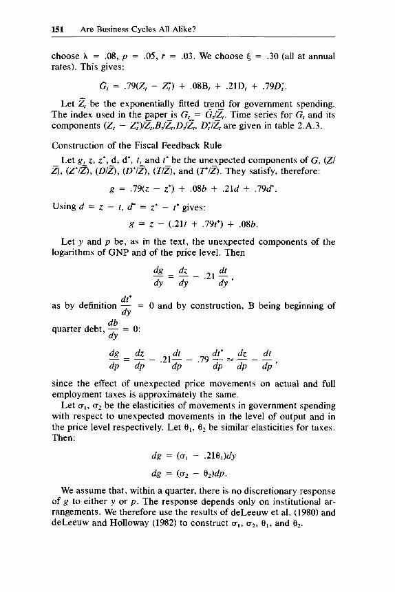
choose A = .08, p = .05, r = .03. We choose ~ = .30 (all at annualrates). This gives:
G, = .79(Z, - Z;) + .08B, + .21D, + .79D;.
Let Z, be the exponentially fitted trend for government spending.The index used in the paper is G, = G,/z,. Time series for G, and itscomponents (Z, - Z;)IZ"B,/Z"D,/Z" D;IZ, are given in table 2.A.3.
Construction of the Fiscal Feedback RuleLet g, z, z*, d, d*, I, and 1* be the unexpected components of G, (ZI
Z), (Z*IZ), (DIZ), (D*IZ), (TIZ), and (TIZ). l~hey satisfy, therefore:
g = .79(z - z*) + .08b + .21d + .79d*.
Using d = z - I, d* = z* - 1* gives:
g = z - (.211 + .791*) -t- .08b.
Let y and p be, as in the text, the unexpected components of thelogarithms of GNP and of the price level. T'hen
dg = dz _ dt.21 dy'dy dy
o and by construction, B being beginning ofb d fi.. dt*
as y e nltlon dy
dbquarter debt, dy = 0:
dg _ dz _dp - dp
21 dt _ 79 dt* ~~ dz _ dl. dp . dp dp dp ,
since the effect of unexpected price movements on actual and fullemployment taxes is approximately the sanle.
Let 0"1, 0"2 be the elasticities of movements in government spendingwith respect to unexpected movements in the level of output and inthe price level respectively. Let 8J, 82 be sirnilar elasticities for taxes.Then:
dg = (0"1 - .21( 1)dy
dg = (0"2 - 62)dp.
We assume that, within a quarter, there is no discretionary responseof g to either y or p. The response depends only on institutional ar-rangements. We therefore use the results of deLeeuw et al. (1980) anddeLeeuw and Holloway (1982) to construct 0"1' 0"2' 8J, and 82 •

152 Olivier J. Blanchard/Mark W. Watson
0"1: From table 19 of deLeeuw et al. (1980), a one percentage pointincrease in the unemployment rate increases spending in the first quarterby 0.6% at an annual rate. From Okun's law it is reasonable to assumethat a 1% innovation in output reduces unemployment by roughly 0.1percentage point in the first quarter. Putting these together we have 0"1
= -0.06.0"2: G is composed of (1) purchases of goods and services, (2) wage
payments to government employees, and (3) transfer payments. Thereis little or no effect of unexpected inflation on nominal purchases withina quarter. Although parts of (2) and (3) are indexed, indexing is notcontemporaneous. Nominal payments for some transfer programs(Medicare, Medicaid) increase with inflation. A plausible range for 0"2
is - 0.8 to - 1.0. We choose - 0.9 for the computations in the text.61: We considered four categories of taxes and income tax bases:(I)
personal income tax; (2) corporate income tax; (3) indirect businesstaxes; (4) social security and other taxes.
We have
T; is available in deLeeuw et al. (1980), table 6, for selected years.T11YiY is available in ibid., table 8.11TIYI is available in ibid., table 10.11T2Y2 is available in ibid., 38, col. 1.11T3Y3 is available in ibid., table 15.11 T4 Y4 is available in ibid., table 18.
We calculated 61 using elasticities and tax proportions for 1959 and1979. The results were very close and yielded 61 = 1.4.
62 : We considered the same four categories of taxes. In the sameway as before, we have
4 T.82 = L T' 11T-Y· 11Y·P;=1 I I I
i is available in deLeeuw et al. (1980), table 6.
11TjYj are given in deLeeuw and Holloway (1982), table 8. (They arelower than the 11T;Y; reported above for the computations of 61.)
11y;p are given in ibid., table 7.We calculated 62 using elasticities and tax proportions for 1959, 1969,
and 1979. The results were very close. A plausible range for 62 (de-

153 Are Business Cycles All Alike?
Table 2.A.3 Fiscal Index and Its Components
Date G (Z-Z*)/Z BIZ DIZ D*IZ
1947: 1 0.238 -0.003 7.788 -0.560 -0.5331947:2 0.225 -0.003 7.521 - 0.515 -0.5271947:3 0.280 -0.003 7.216 -0.396 -0.4501947:4 0.141 -0.003 6.877 -0.523 -0.5501948: 1 0.165 -0.003 6.654 -0.466 -0.5061948:2 0.253 -0.003 6.472 -0.373 -0.3971948:3 0.354 -0.003 6.257 -0.248 -0.2751948:4 0.408 -0.002 6.219 -0.186 -0.2191949: 1 0.447 0.002 6.212 -0.119 -0.1911949:2 0.501 0.012 6.201 -0.030 -0.1531949:3 0.513 0.020 6.144 -0.005 -0.1451949:4 0.486 0.024 6.099 -0.007 -0.1771950: 1 0.582 0.017 6.071 0.007 -0.0501950:2 0.347 0.009 5.976 -0.285 -0.2521950:3 0.218 0.002 5.762 -0.474 -0.3321950:4 0.171 0.000 5.596 -0.477 -0.3671951: 1 0.156 -0.002 5.353 -0.478 -0.3521951:2 0.318 -0.006 5.258 -0.265 -0.1871951 :3 0.459 -0.006 5.187 - 0.111 -0.0411951:4 0.466 -0.004 5.095 -0.056 -0.0361952:1 0.424 -0.006 5.057 -0.093 -0.0731952:2 0.490 -0.006 5.020 -0.014 -0.0061952:3 0.551 -0.006 4.951 0.058 0.0621952:4 0.505 -0.008 4.872 -0.015 0.0341953:1 0.535 -0.009 4.834 0.000 0.0741953:2 0.555 -0.009 4.808 0.033 0.0941953:3 0.513 -0.009 4.768 0.022 0.0491953:4 0.539 -0.002 4.757 0.129 0.0481954:1 0.504 0.009 4.674 0.105 0.0111954:2 0.431 0.012 4.626 0.035 -0.0601954:3 0.409 0.014 4.605 0.009 -0.0801954:4 0.361 0.010 4.539 -0.045 -0.1141955: 1 0.325 0.008 4.462 -0.104 -0.1341955:2 0.276 0.003 4.394 -0.151 -0.1701955:3 0.285 0.002 4.328 -0.148 -0.1501955:4 0.250 0.002 4.246 -0.177 -0.1751956: 1 0.225 0.000 4.156 -0.175 -0.1951956:2 0.225 0.002 4.067 -0.162 -0.1881956:3 0.216 0.001 3.969 -0.151 -0.1901956:4 0.194 0.001 3.884 -0.170 -0.2021957: 1 0.215 0.000 3.793 -0.139 -0.1701957:2 0.224 0.000 3.730 -0.114 -0.1581957:3 0.214 0.001 3.647 -0.114 -0.1621957:4 0.236 0.008 3.621 -0.059 -0.1521958: 1 0.288 0.022 3.586 0.030 -0.1191958:2 0.298 0.035 3.556 0.090 -0.1301958:3 0.361 0.032 3.515 0.088 -0.0421958:4 0.349 0.023 3.481 0.058 -0.0371959: 1 0.258 0.016 3.434 -0.033 -0.115(continued)

154 Olivier J. Blanchard/Mark W. Watson
Table 2.A.3 (continued)
Date G (Z-Z*)/Z BIZ DIZ D*IZ
1959:2 0.208 0.010 3.391 -0.092 -0.1501959:3 0.220 0.011 3.360 -0.056 -0.1421959:4 0.211 0.013 3.317 -0.061 -0.1481960: 1 0.106 0.0q9 3.261 -0.171 -0.2411960:2 0.132 0.010 3.222 -0.126 -0.2161960:3 0.150 0.012 3.176 -0.091 -0.1981960:4 0.160 0.019 3.142 -0.059 -0.1971961: 1 0.195 0.023 3.116 -0.021 -0.1631961:2 0.212 0.025 3.072 -0.012 -0.1411961:3 0.201 0.021 3.029 -0.025 -0.1421961:4 0.204 0.016 3.013 -0.042 -0.1271962: 1 0.241 0.012 2.976 -0.007 -0.0811962:2 0.224 0.011 2.954 -0.025 -0.0941962:3 0.210 0.011 2.936 -0.037 -0.1071962:4 0.205 0.011 2.902 -0.030 -0.1101963:1 0.181 0.012 2.874 -0.050 -0.1321963:2 0.150 0.011 2.857 -0.087 -0.1591963:3 0.162 0.009 2.834 -0.081 -0.1411963:4 0.172 0.009 2.794 -0.068 -0.1261964:1 0.206 0.008 2.767 -0.045 -0.0851964:2 0.240 0.007 2.740 -0.011 -0.0471964:3 0.196 0.005 2.705 -0.049 -0.0861964:4 0.175 0.004 2.680 -0.063 -0.1041965: 1 0.142 0.003 2.639 -0.107 -0.1281965:2 0.149 0.002 2.608 -0.103 -0.1151965:3 0.212 0.000 2.575 -0.044 -0.0461965:4 0.227 -0.001 2.537 -0.044 -0.0221966: 1 0.202 -0.002 2.488 -0.074 -0.0371966:2 0.184 -0.002 2.436 -0.080 -0.0521966:3 0.213 -0.003 2.399 -0.046 -0.0191966:4 0.227 -0.004 2.361 -0.028 -0.0011967:1 0.263 -0.003 2.332 0.022 0.0351967:2 0.263 -0.004 2.310 0.027 0.0371967:3 0.264 -0.004 2.274 0.028 0.0421967:4 0.259 -0.003 2.279 0.019 0.0371968: 1 0.235 -0.003 2.278 -0.005 0.0131968:2 0.257 -0.005 2.277 0.005 0.0401968:3 0.195 -0.005 2.220 -0.057 -0.0151968:4 0.166 -0.006 2.210 -0.077 -0.0441969:1 0.100 -0.006 2.181 -0.144 -0.1061969:2 0.091 -0.005 2.143 - 0.143 -0.1131969:3 0.104 -0.005 2.050 - 0.112 -0.0931969:4 0.095 -0.005 2.041 -0.101 -0.1061970: 1 0.110 -0.005 2.031 -0.070 -0.0941970:2 0.164 -0.003 2.002 -0.004 -0.0411970:3 0.169 0.002 1.958 0.003 -0.0361970:4 0.179 0.006 1.950 0.032 -0.0351971: 1 0.188 0.011 1.953 0.021 -0.0251971 :2 0.210 0.013 1.917 0.050 -0.003

155 Are Business Cycles All Alike?
Table 2.A.3 (continued)
Date G (Z-Z*)/Z BIZ DIZ D*IZ
1971 :3 0.206 0:013 1.910 0.048 -0.0071971:4 0.201 0.014 1.938 0.040 -0.0151972:1 0.166 0.013 1.944 -0.006 -0.0471972:2 0.207 0.012 1.92.3 0.025 0.0001972:3 0.164 0.009 1.88.5 -0.017 -0.0351972:4 0.230 0.007 1.869 0.040 0.0381973: 1 0.180 0.005 1.886 -0.032 -0.0081973:2 0.159 0.004 1.871 -0.042 -0.0281973:3 0.127 0.002 1.817 -0.065 -0.0541973:4 0.128 0.001 1.772 -0.060 -0.0481974:1 0.109 0.000 1.751 -0.056 -0.0701974:2 0.118 0.001 1.707 -0.034 -0.0591974:3 0.086 0.002 1.647 -0.044 -0.0891974:4 0.106 0.006 1.60.5 0.003 -0.0751975: 1 0.146 0.019 1.584 0.076 -0.0541975:2 0.327 0.037 1.599 0.242 0.1121975:3 0.226 0.038 1.62.5 0.132 0.0071975:4 0.218 0.037 1.638 0.122 0.0001976: 1 0.200 0.036 1.67.3 0.088 -0.0171976:2 0.176 0.033 1.706 0.062 -0.0421976:3 0.182 0.030 1.722 0.068 -0.0351976:4 0.191 0.027 1.714 0.077 -0.0221977:1 0.153 0.026 1.722 0.026 -0.0561977:2 0.170 0.022 1.716 0.034 -0.0321977:3 0.200 0.019 1.68.5 0.058 0.0051977:4 0.188 0.018 1.699 0.051 -0.0081978: 1 0.175 0.014 1.699 0.037 -0.0161978:2 0.139 0.010 1.687 -0.016 -0.0431978:3 0.124 0.010 1.658 -0.028 -0.0551978:4 0.118 0.008 1.644 -0.039 -0.0571979:1 0.089 0.007 1.624 -0.062 -0.0841979:2 0.068 0.005 1.59.3 -0.070 -0.1011979:3 0.091 0.005 1.559 -0.048 -0.0741979:4 0.103 0.006 1.550 -0.030 -0.0631980: 1 0.106 0.006 1.540 -0.022 -0.0601980:2 0.117 0.0.3 1.518 0.019 -0.0621980:3 0.125 0.019 1.491 0.035 -0.0581980:4 0.110 0.018 1.487 0.020 -0.0711981: 1 0.062 0.021 1.468 -0.039 - 0.1171981 :2 0.063 0.027 1.480 -0.035 -0.1241981 :3 0.078 0.025 1.442 -0.019 -0.1021981:4 0.099 0.020 1.434 0.024 -0.0811982:1 0.099 0.028 1.446 0.041 -0.0941982:2 0.099 0.035 1.458 0.043 -0.1041982:3 0.146 0.046 1.449 0.094 -0.0681982:4 0.204 0.051 1.502 0.157 -0.022
156 Olivier J. Blanchard/Mark W. Watson
pending on which 'TlTiYi are used) is 0.1 to 0.3. We choose 0.2 for com-putations in the text.
Our fiscal policy rule is therefore: g = - .34y - 1.lp + eg •
Comment Robert J. Shiller
These are intriguing questions: Is the macroeconomy disturbed by verylarge shocks occasionally or by small shocks regularly? Is there a singlesource of shocks to the economy, or are there many? Is the pattern ofbehavior constant through time or changing? These questions are notstated in terms of an explicit model and seem to call for some sort ofexploratory data analysis. The authors have done this in an imaginativeand careful manner, showing thoughtful attention to methods. Theytook the trouble to do Monte Carlo work to get empirical distributionsfor statistics for which no distribution theory is available, to use modemrobust regression techniques instead of the usual ordinary least squares,and even to create new formal techniques that capture some motivationof popular exploratory techniques.
They rightly perceive that to answer the questions posed here onereally would like to have a model of the propagation mechanism forthe shocks. Part of their work involves constructing such a model. Themodel, however, is not used throughout the paper, and some techniquesused here are really in the nature of data description.
The authors refer to a "common framework of analysis" in modemmacroeconomics that uses stochastic difference or differential equa-tions to model the propagation of shocks. This framework is not enoughby itself to suggest any way of studying the kurtosis of the extraneousshocks that strike the economy. We need to know more; we need toknow the structure of the model. We can, of course, observe the re-siduals in an autoregression, as are shown in the authors' table 2.1.But what do these residuals mean? Suppose the true model is a con-tinuous time stochastic differential equation of the form dX!Xt < = dWt
+ .5dl, where Wt is a unit Wiener process. Then X t = c*exp(Wt ) is alognormal variable whose kurtosis increases with t. Here the underlyingshocks are all normal, but the propagation mechanism creates a variableX t with an arbitrarily high kurtosis. (The kurtosis of a lognormal vari-able goes to infinity as the variance of the underlying normal variableis increased to infinity.)
Nor is there any way in the absence of a model to study whetherthe economy is dominated by a single shock or by many shocks. Even
Robert J. Shiller is professor of economics at Yale University.

157 Are Business Cycles All Alike?
if we knew that the vector X t is determined by a first-order vectorautoregression model, we might have problems. Suppose all compo-nents of the vector error term were in fact zero except for the first;that is, the economy is driven by a single shock. That is, X t = BXt - 1
+ U t , where B is a matrix and U t = [Ut" 0]. We could discover that U t
has this special form by regressing X t on X t -1 and looking at the variancematrix of residuals. However, if the special model holds for quarterlydata but we had semiannual data for estimation, we would not observethis special structure for the error term. 'With data for every otherquarter we would observe X t = B2Xt _ 2 + Vt, where V t = Ut + BUt-t.In general, none of the elements of V t will have zero variance.
The model presented here is therefore of primary importance to thepaper. The model is described not inappropriately as a "standard mac-roeconomic model," though not all the c:oefficient restrictions are"standard." The equations look something like standard textbookequations with lagged endogenous variablt~s and error terms added.The policy variables are represented by fiscal and monetary reactionfunctions. The fiscal policy index g is unusual; it is a mixture of gov-ernment expenditure, the national debt, and the deficit.
How are the equations identified? The identifying restrictions arealmost those of the standard recursive model in which the matrix ofcoefficients is triangular and the variance olatrix diagonal. Recall thatin that system the diagonality of the variance matrix is necessary foridentification ofall equations in the model. Also, in the recursive systemall equations can be estimated consistently by ordinary least squares.This system differs from the recursive syste:m only in that the equationthat in the recursive system would contain only one endogenous vari-able is an equation with three endogenous variables but with all of thecoefficients assumed known a priori. This equation is the fiscal policyreaction function, the equation that determines g. The coefficients arespecified before estimation by a clever use of some institutional dataon government reactions. Now the model is identified, but the equationscannot be estimated by ordinary least squares. Since the matrix ofcoefficients of the endogenous variables is not triangular, we mustinstrument the regressions.
Even so, the assumption that the error terms are uncorrelated acrossequations is necessary for identification. I wonder if that is a reasonableassumption. Where did the assumption COlne from? One way of ap-preciating the arbitrariness of such an assumption is to note that if themodel holds for monthly data, say, with error terms uncorrelated acrossequations, then the quarterly data will not generally have a represen-tation with error terms uncorrelated across equations.
Since lack of correlation of residuals across equations was used toidentify the model, it follows that if we doubt these restrictions we can
158 Olivier J. Blanchard/Mark W. Watson
take linear combinations of these equations as we please so long asthese combinations do not violate zero restrictions on the coefficients.The authors are concerned that the coefficient of M in the aggregatedemand equation has the wrong sign. One might, for example, add themoney supply equation to this equation, thereby rectifying the wrongsign.
Another identifying assumption is that monetary policy does notdepend on the contemporary fiscal policy variable. Why is this omitted?Does the Fed always ignore fiscal policy? How much trust do we wishto place in the high kurtosis of the monetary policy error term shownin table 2.4? Without the identifying assumptions above, the error termin the monetary policy equation could be any linear combination of theerror terms in the other equations.
The assumptions used here for estimation might be compared withthose of Hall in this volume (chap. 4). Hall felt that he could find nomore than one truly exogenous variable for estimation of such a model,this variable being his military expenditure variable. The discussion ofhis paper questioned whether even this variable was exogenous. Theassumed exogeneity here of residuals of equations lower in the hier-archy is certainly even more questionable than the assumption madeby Hall.
The authors, inspired by the methods of Burns and Mitchell fordescribing business cycles, offer a formalization of their approach. Asan exploratory technique, the Burns and Mitchell reference cycle ap-proach has apparently had a wide appeal. It was a dominant theme inempirical macroeconomics for at least a decade after their book ap-peared in 1946, and the calculation of the reference cycle dates con-tinues to be a widely publicized activity of the NBER. Like moststatistical methods belonging in the realm of exploratory methods it iscontroversial, and the motivations for the techniques are only intuitive.Blanchard and Watson borrowed from the Burns and Mitchell approachand also modified it.
It is interesting to see a formalization of the reference cycle datingitself. It has sometimes been claimed that, while no simple formula isused to date the reference cycle, in fact a recession is declared when-ever real GNP shows two consecutive quarters of decline. Blanchardand Watson have found that the quarter of a trough can be identifiedinstead as any quarter in which real GNP declined from the previousquarter so that it is at least 0.5% below the previous peak and thenincreased for the each of the next three consecutive quarters.
Rather than present the Burns/Mitchell charts of cyclical patternsthat were used to judge the business cycle pattern of series, the authorsoffer a summary measure. This measure is rather different from Burnsand Mitchell's own "index of conformity," which relied on a sort of

159 Are Business Cycles All Alike?
time deformation that in effect reduced all cycles to the same lengthand that depended only on the directions of change at various phasesof the cycle and not on their magnitude. l~he authors instead presentfor each variable in each cycle five correlation coefficients: cross-correlations between the variable and real GNP contemporaneouslyand for two leads and lags. By fixing the leads and lags in terms ofquarters rather than fractions of cycles, Blanchard and Watson's leador lag may be a much higher proportion of the cycle for short cycles,such as that between 1960:2 and 1982:4, vlhich was only ten quarterslong. The authors' interpretation of the correlation coefficients relieson a sort of approximation whose validity is not independent of thelength of the cycle. A procyclical variable will tend to show a corre-lation pattern that is not quite flat. There is probably a tendency forthe peak of the specific cycle to occur, relative to the reference cycle,as indicated by these leads or lags, but that is not necessarily so. Thereis a fundamental difference between such correlation coefficients andmethods involving identification of peaks and troughs. For example,all these correlations would be about zero for any series that was ninetydegrees out of phase with the business cyclle. These correlations wouldstay zero if the series were to switch sign in another business cycle,and so a dramatic change in the cyclical behavior would not be revealedby a change in correlations.
The correlations seem to serve well enough, however, to show towhat extent the behaviors of the various s(~ries are directly "procycli-cal" or "countercyclical." What is immediately apparent in looking atthe correlation coefficients is that there are not a lot of regular patternsto be seen. There is no series that shows a simple procyclical or coun-tercyclical pattern in all seven cycles.
The authors characterize Burns and Mitchell (who studied cyclesbetween 1854 and 1933) as having found substantially less variation inthe cyclical pattern across cycles. That conclusion may be overstated.In looking at the Burns and Mitchell pictures one usually finds for anyspecific series at least one business cycle ~W'ith an anomalous pattern.Only two of the Blanchard/Watson series appear to correspond ap-proximately to series studied by Burns and :Mitchell: these are the long-term and short-term interest rates. Plots very similar to those of Burnsand Mitchell appear in the Zarnowitz/Moore paper, "Major Changesin Cyclical Behavior" in this volume (chap. 9). Comparing their tables9.3 and 9.6 with their tables 9.4 and 9.7 suggests that conformity tothe cycle has declined since World War II only for the short rate.
Both Blanchard and Watson and Zarnowitz and Moore find that shortrates are procyclical, show good conformity to the cycle, and lag thereference cycle somewhat. Both papers find less conformity of longrates to the cycle. However, Blanchard and Watson find that the long

160 Olivier J. Blanchard/Mark W. Watson
rate is countercyclical and tends to lead the business cycle by at leasttwo quarters. This last conclusion is not in Zarnowitz and Moore. Onemight note that it hardly seems likely that the short rate should beprocyclical and the long rate countercyclical, since the two series arefairly positively correlated. This points up some of the rather importantdifferences between the Zarnowitz/Moore and Blanchard/Watson ap-proaches. The correlation patterns shown in Blanchard and Watson'stable 2.7 are not totally dissimilar for long and short rates, but theiridentification of leads or lags or procyclical or countercyclical behaviordepends on which correlation coefficient is biggest in absolute value.Of course, a procyclical variable that leads the cycle by x degrees canalways be described as countercyclical and as leading the cycle by180 - x degrees. With an average duration of postwar cycles of aboutfour years, such calculations suggest that the long rate leads by overa year, which is beyond the range for which they computed correlationcoefficients. (They could not have computed correlation coefficientsout much further on all cycles, since one postwar cycle is only elevenquarters long.)
The summary statistics provided by Blanchard and Watson, the dif-ference between the maximum and minimum correlation coefficientover the seven cycles, are generally above one for all series but theshort rate. This documents the observation that for most variables thereis at least one business cycle where the variable shows anomalousbehavior.
The authors rightly felt that some sort of significance test for thestatistic was desirable. They wanted to know whether differences ofthis magnitude should be "surprising." They then computed for eachseries an empirical distribution for this statistic for data generated ac-cording to the estimated fourth-order bivariate autoregression repre-sentation for the series and real GNP. Since the null hypothesis for thistest allows a bivariate autoregression process for which the pattern ofcycles may be either usually very similar across cycles or usually verydifferent across cycles, it is not clear in what sense we could expectthe power function for this test to divide important alternativehypotheses.
Comment Peter Temin
The paper by Blanchard and Watson is extremely interesting. Theauthors deserve our thanks for their efforts to take an informal con-
Peter Temin is professor of economics at Massachusetts Institute of Technology.

161 Are Business Cycles All Alike?
troversy in the literature and endow it with enough shape to be testable.As any historian knows, there are pitfalls in that process. But the effortitself is necessary, even ifit only provides a forum for others to disagree.By moving the discussion out of the realm of slogans into the arena oftestable hypotheses, the authors have don(~ a great service.
The question in the title turns out to have two (related) meanings.The obvious meaning, whether all business cycles look alike as theydevelop, is treated in the second part of the paper. A more subtleformulation, whether all business cycles have the same cause, is theconcern of the first part. After a brief comment on the former topic, Iwill concentrate on the latter.
Postwar business cycles, according to Blanchard and Watson, arenot all alike. But, they continue, little information is contained in theirdifferences. These differences do not indicate that business cycles arecaused by identifiable, discrete large shocks. It isjust that the economyis not a tight enough system to force all fluctuations into a single fixedmold. This result then poses a further question for us to ponder-namely, whether the variance Blanchard and Watson found is trulyrandom or the result of a regular process more complex than theirmodel can capture.
Causation of business cycles is treated in an elegant way. The authorsdistinguish between proponents of so-called large-shock theories andsmall-shock theories of business cycles. Large shocks by their natureare identifiable and different one from another; they are the stuff ofeconomic history. Small shocks, by contrast, are nameless and indi-vidually uninteresting. It is only their distribution over time that mattersfor the origin of cycles, which are then produced by the interaction ofthe economy's internal dynamics and the ac~;umulationof small shocks.The shocks that we observe are themselves, the authors imply, thesum of many smaller shocks that we cannot even see in the data, muchless describe or verify from other sources.
My comments will deal both with the authors' methods and withtheir conclusions. I will start with methodology and work towardsubstance.
The first point follows from Blanchard and Watson's interpretationof the imprecise distinction between large~ and small shocks. A dis-covery that the distribution of innovations has fatter tails than a normaldistribution provides evidence of large shocks, in their parlance, butit may not capture the earlier discussion. Disturbances large and in-frequent enough not to be captured by a normal distribution may stillbe too small and frequent to be noted by the proponents of large shocks.In fact, independent one-quarter shocks may be too limited in time tobe counted as large. A different error structure and a different definitionof large might well produce a different answer.

162 Olivier J. Blanchard/Mark W. Watson
The factual basis of this investigation consists of precisely four quar-terly time series. There are casual references to the rest of the world,but this is an exercise undertaken with strict rules. It is like classicalgeometry, in which the student is limited to what he or she can provewith straightedge and compass. Or like black-and-white photographyin which the drama of color is eschewed in favor of a concentrationon light and form. But since, unlike these two examples, there are nogenerally accepted guidelines to indicate which "stylized facts" shouldbe included and which omitted, it is appropriate to ask if the use offour series seems attractive.
One alternative can be rejected immediately. The use of a large fore-casting model would hopelessly complicate the issue without muchanticipation of gain. There are so many errors in those models, withso many special properties, that a simple characterization of them ascoming from a simple, stationary distribution would be impossible.Another alternative, though, appears more attractive. Why not fiveseries, or six? The gains are not as impressive as those claimed by BobSolow in the transition from one-sector to two-sector growth models,but they may not be negligible either. The authors provide us with onecautionary tale along these lines. They say that they cannot decomposeprices into raw materials prices and other prices in order to examinemore closely oil price shocks and related phenomena, because theerrors relating to those shocks cannot be disentangled from other priceshocks. The gain in information is only apparent, not real.
This argument does not seem, at least on its face, to be applicableto the omission of an interest rate, q, or other series reflecting the costof capital. I am prepared to hear that there are good statistical reasonsfor omitting this kind of variable, but it gives me pause. True, theaggregate demand equation is derived from IS and LM curves, and itserrors (innovations) are linear combinations of the errors in the un-derlying IS and LM curves. If errors in these two relationships areuncorrelated, little is lost. But if, as the authors suggest, there is atendency for innovations to cluster in time, the aggregate demand in-novations will miss offsetting innovations in the fiscal and monetaryareas.
Blanchard and Watson, then, limit themselves to a simple aggregatedemand/aggregate supply model. There are two other equations, butthey do not provide additional detail about the functioning of the privateeconomy. They are policy feedback rules. So if we compare this modelwith, say, Klein's simple models of the economy in the infancy ofmodern econometrics, we discover two differences. First, as alreadynoted, it gives explicit attention to both fiscal and monetary innova-tions, even if information about them is limited. And second, it incor-porates rules for government policy formation.

163 Are Business Cycles All Alike?
The second differences affects the identification of shocks no lessthan the first. Monetary and fiscal shocks are deviations from the as-sumed rules of behavior, not from constancy or some smooth path overtime.
The policy rules are themselves of interest. The fiscal rule is cal-culated, not estimated. It reveals a count,ercyclical fiscal policy: au-tomatic stabilizers. The fiscal policy variable was constructed to showvarious effects of government spending and debt. It contains a cyclicalcomponent, and the fiscal policy equation can be thought of as cleansingit. That is, the equation for g separates the normal cyclical movementsof fiscal policy variables from "true shocks." This seems like an awk-ward process in which the cyclical components of fiscal policy are firstbuilt into g by construction and then removed again by calculation. Itwas indicated, apparently, to distinguish changes in discretionary fiscalpolicy from cyclical movements in the gove~rnment budget while allow-ing both to influence subsequent events.
The monetary policy rule, by contrast, is estimated. It shows exactlythe opposite pattern. Whereas fiscal policy was "normally" counter-cyclical, monetary policy was procyclical. It was, in other words, ac-comodating. This is in itself an important conclusion. It may be anaccurate description of monetary policy in the immediate postwar years,but it hardly seems to describe the role of the Fed in recent years. Theuse of a single model for the entire period from 1947 through 1982cannot uncover such a shift. It would be interesting to see what wouldhappen if the sample was broken at some point in time.
This procedure would provide information about changes both inpolicy rules and in shocks. (Were the 1970s really worse than the 1960s?)If there was a structural shift midway through the sample, its absencewould tend to magnify the apparent shocks, particularly at the ends ofthe period. An informal look at table 2.4 suggests that something likethis may indeed be going on.
Examining table 2.4 moves us from methodology to substance. AsBlanchard and Watson comment, the most striking feature of table 2.4(which shows the structural disturbances) is its lack of intuitive appeal.Despite considerable ingenuity, the authors succeed in making only onepositive identification between their calculated innovations and theeconomic history of the postwar years (in 1974-75). I do not countlarge disturbances of one sign followed irrlmediately by equally largedisturbances of the opposite sign or disturbances that can be assignedto a known cause only by Procrustean tailoring of the date. There aresixty large disturbances shown in table 2.4, and it would be surprisingif chance alone did not place a few of thern on the dates of historicalevents. There does not seem to be much correlation between the cal-culated disturbances and our historical memory.

164 Olivier J. Blanchard/Mark W. Watson
This is due partly, no doubt, to the matter of definition and procedurementioned earlier. But to the extent that it is not, this result forces usto choose between the formal history of Blanchard and Watson andthe more informal history ofEckstein and Sinai. How should one choose?
To aid this choice, I compared the structural disturbances in table2.4 with deviations of the four variables from simple time trends. Thedifferences are striking. The large disturbances of table 2.4 do not lookautocorrelated. And the distributions of the four disturbances do notappear very different. Compared with a time trend, however, the vari-ables divide into two clear groups. M1 and the GNP deflator (m andp) have highly autocorrelated disturbances, with little variation fromone quarter to the next. GNP and the fiscal index (y and g), by contrast,have far less autocorrelation and far more quarter-to-quarter variation.
M1 and the GNP deflator grew slower than trend until the late 1960sand faster thereafter. (If one were to break the sample into two, assuggested earlier, the turning point of the later 1960s would be theobvious break point.) Neither of the other variables seems to show abreak in trend at that time, although the fiscal variable appears to havemuch larger (relative) variation than GNP.
This pattern can be discerned in Blanchard and Watson's table 2.3,which decomposes forecast errors of their model. First, it is worthnoting that the policy innovations seem to have little effect on the restof the economy. Fiscal shocks affect the fiscal shock and nothing elsein the next quarter. Even after a year, they have almost no effect onthe other variables. And after five years, the effect of past fiscal shockson current fiscal shocks is over twice as large as its effect on any ofthe other variables. Monetary shocks have exactly the same pattern.After five years, there is some effect of monetary shocks on prices,but the effect is only about half as strong as the effect on money itself.
Second, there is a sharp separation between the effect of supply anddemand shocks. Supply shocks affect prices, and demand shocks affectoutput. This is true in the next quarter and remains largely true aftera year. (Demand shocks have noticeable effects on prices by then,although supply shocks still dominate.) Only after five years do pricesand income appear to be affected by a mixture of influences.
In the short run, therefore, Blanchard and Watson's economy has aroughly horizontal aggregate supply curve and a roughly vertical ag-gregate demand curve. As the authors note, this conclusion is stronglyaffected by their derivation from the fiscal equation. They presentalternative structural estimates of their model in appendix 2.1, basedon different calculated values of the price responsiveness of the fiscalstimulus. They allow the coefficient of p in the fiscal equation to varyfrom 1.0 to 1.3. This makes the price coefficient in the supply equationvary from 0.45 to 1.40---a threefold variation. It follows that the par-

165 Are Business Cycles All Alike?
ticular short-run characterization of the economy given by Blanchardand Watson may not be the only reasonable description. This in turnimplies that the pattern of variances shown in table 2.3 may not be theonly one generated by reasonable constructions of the economy.
In the long run this model appears to give more conventional results,showing the joint effect of all the shocks cited. A note of caution maybe injected, however, in the use of a very simple model like this oneto project the effect of errors over fifty years. The last section of table2.3 may only be telling us that the relations estimated in table 2.2 aretoo simple to use in projecting an economy over five years. The authorsuse this kind of model to look at the short-run errors; there is no reasonto think it is the best way to approach problern.s of longer-run forecasting.
Blanchard and Watson therefore seem to be presenting us with aneconomy that, at least in the short run, decomposes into several ratherindependent subeconomies. This surely is different from the economydescribed by Eckstein and Sinai. It also may well depend on the par-ticular derivation used, as suggested by the alternatives furnished inappendix 2.1. The principal issue they raise, therefore, may not bewhether shocks to the economy are generated by a normal distribution,but rather whether the short-run responsiveness of the economy hasthe simple structure they have attributed to it.
Discussion Summary
The discussion began with a response by Sims to Shiller's commentsregarding identification and exogeneity. Sims stated that the identifi-cation of any stochastic model requires that restrictions be placed onthe model's error process. Usually investigators make assumptionsabout the exogeneity of certain variables entering the model. Blanchardand Watson's approach, however, is to regard nothing as totally ex-ogenous. This forces them to turn to exclusion restrictions and explicitassumptions on the error terms, in particular a diagonal covariancematrix for the contemporaneous shocks, to achieve identification. Shill-er's point that the use of the wrong sampling period can induce con-temporaneously correlated errors applies equally to incorrect identi-fying restrictions. Such a criticism does not mean that identificationshould not be attempted; it means only that identifying restrictionsshould be used wisely, as Blanchard and Watson have done. FinallySims drew attention to the sophisticated extension ofVAR methodologyused by this paper. A vector autoregression was first used to generate"reduced form" residuals. Robust simultaneous equation estimation

166 Olivier J. Blanchard/Mark W. Watson
techniques were then used to transform the reduced-form shocks intoshocks arising from a structural model.
Although McCallum felt that the large-shock versus small-shock viewof impulses was valuable, he questioned the authors' statements onthe associated policy implications. McCallum said he could see noreason why the presence of small shocks necessarily supported policyrules or why large shocks necessarily led to a need for discretionarypolicy. In reply, Blanchard referred McCallum to the debate betweenRobert Lucas and Robert Solow in Rational Expectations and Economic Policy (Fischer 1980, 249-64). Blanchard felt that the prevailingview of the profession, as espoused by Solow, seemed to be that largeshocks were unique events whose source could be readily identifiedand counterbalanced with specific policies. The sources of small per-turbations were harder to isolate, and this argued for built-in automaticstabilizers to offset their effects. Finally, several participants remarkedthat there might be difficulties in differentiating between true smallshocks and a large shock that came in as a succession of small shocksbecause of the choice of the sampling interval. Blanchard concededthat this was a,potential problem, but held that the eight-quarter fore-cast decompositions of GNP presented in table 2.A.2 did not seem toindicate that this was the case here.
Additional ContributionAre Business Cycles Symmetrical?J. Bradford DeLong and Lawrence H. Summers
1. IntroductionThe dating of peaks and troughs and the concomitant emphasis on
the different qualitative mechanisms involved in cyclical expansionsand contractions have been major features of the NBER program onbusiness cycle research. Asymmetry between expansions and con-tractions has long been a focus of such research. Thus Wesley Mitchellwrote (1927), "the most violent declines exceed the most considerableadvances .... Business contractions appear to be a briefer and moreviolent process than business expansions." Keynes wrote in the General Theory (1936) that "the substitution of a downward for an upwardtendency often takes place suddenly and violently. . . no such sharp
J. Bradford DeLong is a graduate student in the Department of Economics at HarvardUniversity. Lawrence H. Summers is professor of economics at Harvard University.
We wish to thank the National Science Foundation for financial support.

167 Are Business Cycles All Alike?
turning point occurs when an upward is substituted for a downwardtendency." Indeed Neftci (1984) states that "the claim that major eco-nomic time series are asymmetric over different time phases of thebusiness cycle arises in almost all major works on business cycles."
In many respects the techniques of modern statistics and econo-metrics surely supersede earlier methods of cyclical analysis. Theymake possible the application of techniques of statistical estimationand inference. They remove the need for judgment in data description.And they provide a rigorous basis for nOQjudgmental forecasting. Yetstatistical models of the sort used in economics-whether built in thestructural spirit of the Cowles Commission or in the modern time seriestradition-are entirely unable to capture cyclical asymmetries. If, asKeynes, Mitchell, and others belived, cyclical asymmetries are of fun-damental importance, then standard statistiical techniques are seriouslydeficient. Something like traditional business cycle analysis may thenbe necessary to provide an adequate empiri(;al basis for theorizing aboutcyclical behavior.
Hence the question of the magnitude of cyclical asymmetries seemsto be of substantial methodological importance. Yet with the exceptionof the work of Neftci (1984), it appears to have attracted relatively littleattention. This paper examines the extent of cyclical asymmetries usingAmerican data for the prewar and postwar periods and data on fiveother major OECD nations for the postwar period. We find no evidenceof asymmetry in the behavior of GNP or industrial production. For theUnited States only, we find evidence of some asymmetry in the behaviorof unemployment. We conclude that asymInetry is probably not a phe-nomenon of first-order importance in understanding business cycles.It appears that there is not much basis for preferring some version oftraditional cyclical techniques of analysis and forecasting to more sta-tistical methods.
Section 2 of this note describes our methods and presents the resultsof our analysis of GNP and industrial production. Section 3 followsNeftci (1984) in considering unemployment. We note some method-ological problems we have with his analysis and then show that hisconclusions about the behavior of unemployment appear to be invalidoutside the United States. Section 4 provides some brief conclusions.
2. Asymmetries in Output?The essence of the claims of Keynes and Mitchell quoted in the
previous section was that economic downturns are brief and severerelative to trend, whereas upturns are longer and more gradual. Thishypothesis has a clear implication: there should be significant skewnessin a frequency distribution of periodic gro\vth rates of output. That is,the distribution should have significantly fewer than half its observa-

168 Olivier J. BlanchardIMark W. Watson
tions below the mean; and the average deviation from the mean of theobservations below the mean should be significantly more than theaverage deviation of the observations above the mean. The medianoutput growth rate should exceed the mean by a significant amount.Figure C2.1 depicts the predicted frequency distribution of output growthunder the null hypothesis of symmetry and under the alternative hy-pothesis of Keynes and Mitchell.
Our procedure is simple: it is to calculate the coefficient of skewnessof the distribution of output growth rates for a variety of output mea-sures and time intervals. The coefficient of skewness is defined as theratio of the third centered moment to the cube of the standard deviation.For a symmetric distribution, the coefficient of skewness is zero, andthe mean equals the median.
4
......···.....................
o 2
...............
.
.
-2
0.75
0.25
1.00----------.........-:.-.. ------------,...........
.... ..
--. --.O.OO'--.-.:::::::~--..L-------L.-----~--~ .............,
-4
0.50
Fig. C2.1 Standardized (zero mean and unit variance) distribution withzero and unit skewness, respectively.

169 Are Business Cycles All Alike?
Evaluation of the statistical significance of any measured deviationsfrom symmetry clearly requires an estimate of the sampling variabilityin our estimates of skewness. Standard statistical works such as Ken-dall and Stuart (1969) note that under the null hypothesis of zero skew-ness, the estimated skewness of a set of n independent random normalobservations is normally distributed with a standard error of (6/n)V2•
Unfortunately, the observations on growth rates considered here arehighly serially correlated, and so this formula is inapplicable. We there-fore used the following Monte Carlo procedure for each series andsample period considered. First, a third-order autoregression processwas estimated for the time series of growth rates. It was then used togenerate three-hundred artificial series for the sample period under theassumption that the shocks to the autoregression process were normallydistributed. The standard deviation of the lestimated skewness underthe null hypothesis was then used calculated as the standard deviationof the skewnesses of the artificially generated series. l
Table C2.1 presents some evidence on skewness in quarterly andannual growth rates of United States GNP and industrial production
Table C2.1 Skewness of United States GNP and Industrial Production GrowthRates
Annual Data Quarterly Data
Standard StandardVariable Period Skewness Error Skewness Error
GNP 1891-1915 - .47 .73 .55 .29GNP 1923-40 - .70 1.12 .04 .42GnP 1949-83 -1.37 .74 -.33 .29IP 1949-83 - .55 .68 -.58 .40
Source: Data from Gordon 1982 and from the 1984 Business Conditions Digest.
1. We verified that the estimated skewnesses were approximately normally distributed.Coefficients of kurtosis were less than 10% away frotTI their value of three under thenull hypothesis. Note that our test of asymmetry is appropriate if output is stationaryeither when detrended or when differenced. Our standard errors are calculated underthe second assumption, which is weakly supported by ~~elson and Plosser 1982. Becausethey include periods in their analysis like the Great Depression and World War II, duringwhich no one would expect the underlying rate ofgrowth of the economy to stay constant,it is hard to interpret how their warnings against the practice of detrending apply toanalyses that deal only with periods for which one has good reason to suspect that theunderlying growth of potential output has been approximately constant.
For the United States industrial production index, estimated skewnesses for subperiodsof the post-World War II period are highly variable-Inore variable than the stochasticerrors calculated under the assumption of an AR(3) generating process would suggest.Apparently, modeling the generating process as an AR(3) does not capture all the serialdependence in the series and leads to estimated standard errors that are presumably toolow. Therefore the standard errors reported in this paper are probably below their actualvalues.

170 Olivier J. Blanchard/Mark W. Watson
for various sample periods. We use industrial production as well asGNP because the latter contains a greater number of imputed series,and because cyclicality is most apparent in the manufacturing sectorof the economy. Because using quarterly data is complicated by theneed for seasonal adjustment and by high-frequency movements thatmight render existing skewness undectable, both annual and quarterlydata are examined.
Very little evidence of significant asymmetries emerges. Before WorldWar II, quarterly GNP growth rates exhibit positive skewness, theopposite of that implied by the hypotheses of Keynes and Mitchell.The failure of the steep 1929-33 decline to dominate the interwar periodis somewhat surprising. We expected significant skewness to be mostapparent around the Great Depression. Similar conclusions are ob-tained with annual GNP data and with data on annual industrial pro-duction for the prewar period. Asymmetries do not appear to be sub-stantial enough to be important. The difference between the medianand mean growth rates reaches a maximum of 0.3% using quarterlydata on industrial production for the postwar period. This differenceis only 2% of the interquartile range of the distribution of quarterlygrowth rates: it is a very small number.
There is a little bit of evidence in favor of skewness in postwar data.All the estimated skewnesses are negative, as predicted by Keynes andMitchell. In the case of annual GNP data, the estimated skewnessapproaches statistical significance. However, no equivalent result isfound with either quarterly GNP or annual industrial production data.Hence we are inclined to discount its significance. It is of course pos-sible that with longer time series significant asymmetries would emerge-the estimate of skewness would become sharper. But as figure C2.2reveals, the observed skewness does not appear to be substantivelyimportant. The naked eye cannot easilyjudge the direction ofasymmetry.
As a further check, table C2.2 reports estimated skewnesses of quar-terly GNP and industrial production for other major OECD countriesfor the postwar period. Skewness is noticeably negative for only twoof the five countries-Canada and Japan-using either industrial pro-duction or GNP data. There is no significant evidence of asymmetryfor any country. The only natural grouping suggested by the data is apossible division into the United States, Canada, and Japan on the onehand and the United Kingdom, France, and West Germany on the other.But this possible difference between "non-European" and "Euro-pean" business cycles is not strongly enough present in the data togive us any confidence that it is anything more than the workings ofchance.
How has the picture of recessions as short violent interruptions ofthe process of economic growth emerged? Part of the answer lies in

171 Are Business Cycles All Alike?
28...------------------------
21
(J)
'-cv....'-0:::3
0~
0 14'-cv.0E:::3Z
7
25155-5o--_.....&-...a......&~__L.~ ___L.__,_ ___&..._'__I_...a.__..&.....L. __I
-15
Fig. C2.2 Histogram of quarterly GNP growth rates, 1949-82.
Table C2.2 Skewness of Quarterly Changes in (:iNP and Industrial Production,1950-79
Industrial Production GNP
Standard StandardCountry Skewness Error Skewness Error
United States -.61 .42 - .33 .29Japan -.66 .40 -.43 .29Canada -.52 .39 -.42 .30West Germany -.01 .34 -.11 .26United Kingdom .13 .35 .61 .27France .27 .33 -.03 .24
Source: Data from the OECD Historical Statistics and from the 1984 Business ConditionsDigest.
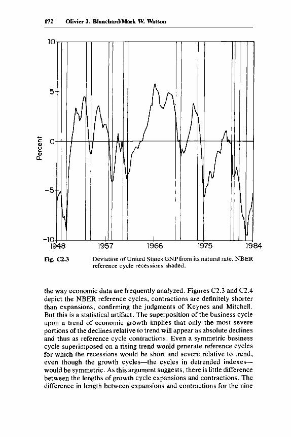
172 Olivier J. Blanchard/Mark W. Watson
lO-r--r---------........-.----.r--T---------.-----...,.....---~~-
5
+-
~ 0o'-Q)a.
-5
-10-t-'- ..--.L...-""------+-'L.",.,I,---I-...t..---+---.......L......L.--L..-.+------L............--!..--.I
1948 1957 1966 1975 1984
Fig. C2.3 Deviation of United States GNP from its natural rate. NBERreference cycle recessions shaded.
the way economic data are frequently analyzed. Figures C2.3 and C2.4depict the NBER reference cycles, contractions are definitely shorterthan expansions, confirming the judgments of Keynes and Mitchell.But this is a statistical artifact. The superposition of the business cycleupon a trend of economic growth implies that only the most severeportions of the declines relative to trend will appear as absolute declinesand thus as reference cycle contractions. Even a symmetric businesscycle superimposed on a rising trend would generate reference cyclesfor which the recessions would be short and severe relative to trend,even though the growth cycles-the cycles in detrended indexes-would be symmetric. As this argument suggests, there is little differencebetween the lengths of growth cycle expansions and contractions. Thedifference in length between expansions and contractions for the nine

173 Are Business Cycles All Alike?
1984197519661957
-5
5
10
-1 0 .....--..L..-.-.I...........,.,""""'--"""---+-~-I.-..&-....L_..J-.-+L-......L...-..L.._..L-~---+-_...&.-_---""-~
1948
.-c~ 0~
Q)
a..
Fig. C2.4 Deviation of United States GN"P from its natural rate. NBERgrowth cycle recessions shadf~d.
growth cycles averaged 0.9 quarters; the standard deviation of thisestimate of the average is 1.4 quarters. 2 By contrast, the average lengthof the seven reference cycle expansions was 11.4 quarters longer thanthe length of the subsequent contractions.3
We conclude from this investigation that once one takes proper ac-count of trend growth-using either our sk,ewness-based approach or
2. We are assuming that each postwar business cycle is an independent draw from apopulation characterized partly by the difference in le:ngth between the expansion andthe recession phase. Cycle dates are taken from Moore and Zarnowitz's "The Devel-opment and Role of the National Bureau of Economic Research's Business Cycle Chro-nologies" (appendix A to this Volume). Note that, as Moore and Zamowitz report, itwas not always the case that expansions were as a rule longer than contractions.
3. With a standard error of the mean of 3.3 quarters. Excluding the highly anomalous1961-70 reference cycle, the mean difference is 8.1 quarters, and its standard error is1.8 quarters.

174 Olivier J. Blanchard/Mark W. Watson
the traditional NBER cycle dating approach-little evidence remainsof cyclical asymmetry in the behavior of output. The impression to thecontrary that we used to hold seems to result from a failure to takeaccount either imrpessionistically or quantitatively of the effects oflong-run economic growth. Few extant theories suggest that businesscycles should depend on the rate of underlying growth of either pro-ductivity or population.4 The next section considers whether similarconclusions are obtained using data on unemployment.
3. Asymmetries in Unemployment?Our conclusions so far contradict those of Neftci (1984), who ex-
amines the behavior of the unemployment rate and finds evidence againstthe null of symmetry at the .80 level. Neftci's statistical procedureseems inappropriate to us: eliminating the quantitative information inthe data by reducing it to a series of ones (unemployment increasing)and zeros (unemployment decreasing) cannot lead to a test of maximumpower.
Table C2.3 presents estimates of the skewness in detrended unem-ployment rates for the United States and other major OECD countriesfor the postwar period. We examine only the postwar data becauseearlier unemployment estimates are in general not derived indepen-dently from output data. For the United States, we confirm Neftci'sconclusion. Indeed, we are able to reject the null hypothesis of sym-metry at the .95 level. Annual data suggest as much skewness as quar-terly data, but the skewness in annual data is not statistically significant.
None of the other OECD countries, however, have statistically sig-nificant skewnesses in their detrended unemployment rates. 5 This sug-gests that skewness in the United States is either a statistical accidentor a result of a peculiarity in the United States labor market. Asym-metry in changes in unemployment rates is not a strong general featureof business cycles.
We have briefly attempted to examine the reasons for asymmetry inAmerican unemployment rates. Skewness does not arise from the be-havior of labor force participation: labor force participation rates ex-hibit no noticeable skewness, and skewness is present in detrended
4. But see Schumpeter 1939 for arguments that the cyclical variance of output is itselfpositively related to the rate of long-run growth.
5. Detrending European unemployment rates is not easy: there appears to have beenan enormous rise in structural unemployment rates all over Europe in the past ten years.The results reported used a second-degreee polynomial to detrend the data. The resultswere effectively unchanged when a third- or a fourth-degree polynomial was used orwhen a piecewise linear trend with a breakpoint in 1973 was used. If the rise in unem-ployment is attributed entirely to cyclical factors-if the skewness of raw changes iscalculated-then changes in European unemployment rates since 1970 appear stronglyskewed.

175 Are Business Cycles All Alike?
Table C2.3 Skewness of Quarterly Changes in Unemployment Rates, 1950-79
Country Skewness Standard Error
United StatesJapanCanadaWest GermanyUnited KingdomFrance
1.03.40.55
- .13.27.14
.30
.28
.29
.27
.30
.33
Source: Data from the 1984 Business Conditions Digest.
Ee~
....c:~
E~
o
-1.6 ~~c::J
8
-:;::- -16----------------------...., 3.2 ~c:~ '0~ ~
~ ~~ ~
~ 2c c:~ ~
~ 0
E -8 1.6 Q;o ~~
~ ~
c:Q)~....
~ ~o 0
g c:~ 0
.~ 16~ ....L_ __L_ __L ---I-3.2 ~~ 1948 1956 1964 1972 1980 ~
Fig. C2.5 United States industrial production and unemployment,1948-80.
unemployment numbers as strongly as in detrended unemploymentrates. Moreover, quarterly changes in employment over the period1949-82 exhibit a skewness coefficient of - 1.90, significant at the .95level. Skewness in employment and unemployment but not in GNPclearly indicates a breakdown in Okun's law. In figure C2.5, inverted
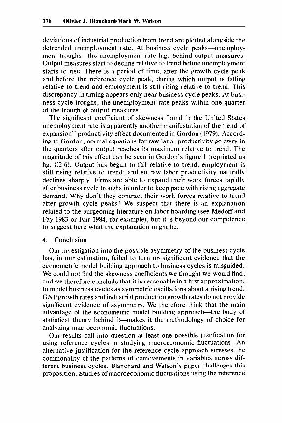
176 Olivier J. Blanchard/Mark W. Watson
deviations of industrial production from trend are plotted alongside thedetrended unemployment rate. At business cycle peaks-unemploy-ment troughs-the unemployment rate lags behind output measures.Output measures start to decline relative to trend before unemploymentstarts to rise. There is a period of time, after the growth cycle peakand before the reference cycle peak, during which output is fallingrelative to trend and employment is still rising relative to trend. Thisdiscrepancy in timing appears only near business cycle peaks. At busi-ness cycle troughs, the unemployment rate peaks within one quarterof the trough of output measures.
The significant coefficient of skewness found in the United Statesunemployment rate is apparently another manifestation of the "end ofexpansion" productivity effect documented in Gordon (1979). Accord-ing to Gordon, normal equations for raw labor productivity go awry inthe quarters after output reaches its maximum relative to trend. Themagnitude of this effect can be seen in Gordon's figure 1 (reprinted asfig. C2.6). Output has begun to fall relative to trend; employment isstill rising relative to trend; and so raw labor productivity naturallydeclines sharply. Firms are able to expand their work forces rapidlyafter business cycle troughs in order to keep pace with rising aggregatedemand. Why don't they contract their work forces relative to trendafter growth cycle peaks? We suspect that there is an explanationrelated to the burgeoning literature on labor hoarding (see Medoff andFay 1983 or Fair 1984, for example), but it is beyond our competenceto suggest here what the explanation might be.
4. ConclusionOur investigation into the possible asymmetry of the business cycle
has, in our estimation, failed to turn up significant evidence that theeconometric model building approach to business cycles is misguided.We could not find the skewness coefficients we thought we would find;and we therefore conclude that it is reasonable in a first approximation,to model business cycles as symmetric oscillations about a rising trend.GNP growth rates and industrial production growth rates do not providesignificant evidence of asymmetry. We therefore think that the mainadvantage of the econometric model building approach-the body ofstatistical theory behind it-makes it the methodology of choice foranalyzing macroeconomic fluctuations.
Our results call into question at least one possible justification forusing reference cycles in studying macroeconomic fluctuations. Analternative justification for the reference cycle approach stresses thecommonality of the patterns of comovements in variables across dif-ferent business cycles. Blanchard and Watson's paper challenges thisproposition. Studies of macroeconomic fluctuations using the reference

177 Are Business Cycles All Alike?
1.20...----------------.--.......
Post-sampleperiod
........ .....~. .~ ., \\!. ~ .I \ •
\\ I~
1975 1977 1979over potential output
Predicted) includingend- of- expansion effect;s;::
: ~l'
Predicted) excludingend of expansion '\. ;~
eftect \... I,'....:1 ~ ••••
: I .,; I •••• 1 I.:/
•• I:,:':1
:1:,: I:,.
• I... ,: I: ,
: • I:~:I: -;1. ...' .•...•.
•••..,
1.10
1.05
1.15
Fig. C2.6 Output per hour in the nonfarrrl business sector, actual andpredicted from alternative equations, 1969:2 to 1979:3. Re-printed from Gordon 1979.

178 Olivier J. Blanchard/Mark W. Watson
cycle approach are the foundation of empirical macroeconomics. Butgiven the availability of modem statistical methods, there appears tobe no scientific basis for the use of reference cycles in either macro-economic analysis or forecasting. As yet, no phenomenon or regularityhas been adduced that can be studied using the reference cycle ap-proach but is inconsistent with the assumptions of standard time seriesmethods. Until such a demonstration is provided, there is little justi-fication for the continued use of reference cycles in studying or fore-casting macroeconomic fluctuations.
References
Adelman, Irma, and Frank L. Adelman. 1959. The dynamic propertiesof the Klein-Goldberger model. Econometrica 27: 598-625.
Blanchard, O. J. 1983. An index of fiscal policy. Mimeographed, Mas-sachusetts Institute of Technology.
---. 1985. Debt, deficits and finite horizons. Journal of PoliticalEconomy 93:223-47.
Brunner, Karl, and Allan Meltzer. 1978. The problem of inflation. Car-negie-Rochester Conference Series on Public Policy 8. Amsterdam:North-Holland.
Burns, A., and W. C. Mitchell. 1946. Measuring business cycles. NewYork: National Bureau of Economic Research.
deLeeuw, F., T. M. Holloway, D. G. Johnson, D. S. McClain, andC. A. Waite. 1980. The high-employment budget: New estimates,1955-1980. Survey of Current Business 60 (November): 13-43.
deLeeuw, F., and T. M. Holloway. 1982. The high employment budget:Revised estimates and automatic inflation effects. Survey ofCurrentBusiness 62 (April): 21-33.
Engle, R. F. 1982. Autoregressive heteroskedasticity with estimates ofthe variance of United Kingdom inflation. Econometrica 50: 987-1008.
Fair, Ray C. 1984. Excess labor and the business cycle. Working Paper1292, National Bureau of Economic Research.
Fischer, Stanley. 1980. Rational expectations and economic p(llicy.Chicago: University of Chicago Press.
Frisch, R. 1933. Propagation problems and impulse problems in dy-namic economics. In economic essays in honor of Gustav Cassel.London: George Allen.
Gordon, Robert J. 1979. The" end-of expansion" phenomenon inshort-run productivity behavior. Brookings Papers on Economic Activity 10: 447-62.

179 Are Business Cycles All Alike?
---. 1982. Price intertia and policy ineffectiveness in the U.S., 1890-1980. Journal of Political Economy 90:6.
Hansen, A. H. 1951. Business cycles and national income. New York:Norton.
Hayashi, F. 1982. The permanent income h.ypothesis: Estimation andtesting by instrumental variables. Journal of Political Economy 90(October): 895-916.
Kendall, Maurice, and Alan Stuart. 1969. J'he advanced theory of statistics. 3 vols. London: McGraw-Hill.
Keynes, J. Maynard. 1936. The general theory ofemployment, interestand money. London: Macmillan.
Krasker, W. A., and R. E. Welsch. 1982. ]~fficient bounded-influenceregression estimation. Journal of the Anlerican Statistical Association 77: 595-604.
Lucas, Robert E. 1977. Understanding business cycles. In Stabilizationof the domestic and international economy, 7-29. Carnegie-RochesterConference Series on Public Policy 1. Amsterdam: North-Holland.
Mitchell, Wesley C. 1927. Business cycles: The problem and its setting.New York: National Bureau of Economic Research.
Medoff, James L., and John A. Fay. 1983. Labor and output over thebusiness cycle: Some direct evidence. M[imeographed.
Moore, Geoffrey, ed. 1961. Business cycle indicators. New York: Na-tional Bureau of Economic Research.
Neftci, Salih N. 1984. Are economic time-series asymmetric over thebusiness cycle? Journal of Political Economy 92:21.
Nelson, C. R., and C. I. Plosser. 1982. Trends and random walks inmacroeconomic time-series. Journal of Jvfonetary Economics 10:2.
Schumpeter, Joseph A. 1939. Business cycles. New York: McGraw-Hill.
Slutsky, E. 1937. The summation of randolm causes as the sources ofcyclic processes. Econometrica 5: 105-46.
