Arctic sea ice and the Atlantic meridional overturning circulation

(AMOC) in a warming climate

Wei Liu

University of California Riverside

June 18, 2019

Collaborated with Alexey Fedorov (Yale)

& Florian Sévellec (Univ.-Brest IRD & U. Southampton)

2

Arctic sea ice decline and AMOC weakening

Sévellec, Fedorov & Liu (2017)

Srokosz and Bryden (2015)

Data from National Snow and Ice Data Center (NSIDC)

NATURECLIMATECHANGEDOI: 10.1038/ NCLIMATE2554 ARTICLES

with the EIV method using all the available proxies, which is thereconstruction for which the best validation results were achieved(see Supplementary Methods of Mann et al.12). Based on standardvalidation scores(Reduction of Error and Coefficient of Efficiency),this series provides a skilful reconstruction back to AD 900 andbeyond (95%significancecompared to ared-noisenull).

The subpolar-gyre series is derived from a spatial temperaturereconstruction13, which reconstructs land-and-ocean surfacetemperatures in every 5◦ latitude by 5◦ longitude grid box withsufficient instrumental data to perform calibration and validation.The subpolar gyre falls within the region where the individualgrid-box reconstructions are assessed to be skilful compared to ared-noisenull13. In addition, weperformed validation testingof thesubpolar-gyremean series, which indicatesaskilful reconstructionback to AD 900 (95%significancecompared to a red-noisenull; seeSupplementary Information for details).

Both timeseriesaswell astheresulting AMOC index areshownin Fig. 3. Remarkably, the subpolar gyre reaches nearly its lowesttemperatures of the past millennium in the late twentieth century(orangecurve), despiteglobal warming. Mann et al.13 already notedthat thisregion near Greenland isanomalousin beingcolder duringthe modern reference period (1961–1990) than even in the LittleIce Age (LIA). The AMOC index (blue curve) indicates a steadyAMOC, with modest changes until the beginning of the twentiethcentury. There is indication of amaximum in the fifteenth centuryand a minimum around AD 1600. There is no sign in our indexthat a weak AMOC caused theLIA in theNorthern Hemisphere14;rather the data are consistent with previous findings that theLIA reflects a response to natural volcanic and solar forcing15–17,and if anything this surface cooling strengthened the AMOC atleast during the first part of the LIA. The fact that LIA coldnessseems to have been even more pronounced in South Americathan in Europe18 further argues against a weak AMOC, as thelatter would havewarmed theSouthern Hemisphere. Thetwentiethcentury shows a gradual decline in the AMOC index, followed bya sharp drop starting around 1970 with a partial recovery after1990 (discussed further below). Thisrecovery isconsistent with thefindingof an AMOCincreasesince1993based on floatsand satellitealtimeter data19.

Our temperature reconstruction for the subpolar gyre differsfrom three estimates based on ocean sediment cores from theregion20,21. However, reconciling these cores with each otherand with the instrumental SST record proves problematic (seeSupplementary Information), whereasour reconstruction compareswell with theinstrumental dataduring theperiod of overlap.

Spectral analysis50 of theAMOCindex indicatesafewmarginallysignificant peakswith periodsaround 22, 27and 37 years, but thesefeaturesarenot clearly discernible from theexpectationsof simplered noise (Fig. 4). We find no significant peak in the 50–70-yearperiod range although our index should pick this up10, suggestingthat the ‘Atlantic Multidecadal Oscillation’ (AMO) described inpreviousstudies22–24 isnot aprominent featureof our AMOC indextimeseries.

The twentieth-century AMOCweakeningThe most striking feature of the AMOC index is the extremelylow index values reached from 1975 to 1995. It is primarily thisnegative anomaly that yields the cooling patch in the trend mapsillustrated in Fig.1. In thefollowingwediscussthisdownward spikein moredetail.

The significance of the 1975–1995 AMOC index reductionwas estimated using a Monte Carlo method (see SupplementaryInformation). The annually resolved AMOC reconstruction from900to1850formed thebasisfor an ARMA(1,1) model which closelyresemblesthestatistical propertiesof thedata.10,000simulated timeseriesof thesamelength astheAMOC index wereconstructed. The

−1

0

1

2

0

a

b

1

2

3

1000 1200 1400 1600 1800 2000

Tem

pera

ture

anom

aly

(K

)Tem

pera

ture

anom

aly

(K

)

Year AD

1000 1200 1400 1600 1800 2000

Year AD

NH + 3 K

Instrumental

Subpolar gyre

Instrumental

Subpolar gyre minus NH

Instrumental

Figure 3 | Surface temperature time series for di erent regions. Data from

the proxy reconstructions of Mann et al.12,13, including estimated 2-σ

uncertainty bands, and from the HadCRUT4 instrumental data49 . The latter

are shown in darker colours and from 1922 onwards, as from this time on

data from more than half of all subpolar-gyre grid cells exist in every month

(except for a few months during World War II). The orange/ red curves are

averaged over the subpolar gyre, as indicated on Fig. 1. The grey/ black

curves are averaged over the Northern Hemisphere, o set by 3K to avoid

overlap. The blue curves in the bottom panel show our AMOC index,

namely the di erence between subpolar gyre and Northern Hemisphere

temperature anomalies (that is, orange/ red curves minus grey/ black

curves). Proxy and instrumental data are decadally smoothed.

probability of reaching a similarly weak AMOC index as during1975–1995 just by natural variability was found to be < 0.005,based on the uncertainty of the proxy data and ignoring that thisweakening is independently supported by instrumental data.

Figure 5 illustrates corroborating evidence in support of atwentieth-century AMOC weakening. The blue curve depicts theAMOC index from Fig. 3. The dark red curve illustrates thecorresponding index based on the instrumental NASA GISSglobaltemperature analysis. The green curve denotes oceanic nitrogen-15 proxy data from coralsoff the USnorth-east coast from ref. 25.These annually resolved δ15N data represent a tracer for water

NATURECLIMATECHANGE | VOL 5 | MAY 2015 | www.nature.com/ natureclimatechange 477

© 2015 Macmillan Publishers Limited. All rights reserved

Rahmstorf et al. (2015)

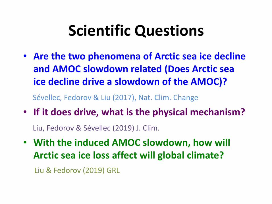
Scientific Questions

• Are the two phenomena of Arctic sea ice decline and AMOC slowdown related (Does Arctic sea ice decline drive a slowdown of the AMOC)?

Sévellec, Fedorov & Liu (2017), Nat. Clim. Change

• If it does drive, what is the physical mechanism?

Liu, Fedorov & Sévellec (2019) J. Clim.

• With the induced AMOC slowdown, how will Arctic sea ice loss affect will global climate?

Liu & Fedorov (2019) GRL

Adjoint analysis: AMOC sensitivity to global surface heat

and freshwater fluxes

Sévellec, Fedorov & Liu (2017)

CESM1 experiments: forcing Arctic sea ice decline

Arctic sea ice decline drives a slow-down of the AMOC.

Liu, Fedorov & Sévellec (2019)

6

Mechanisms

Liu, Fedorov & Sévellec (2019)

Climate response to Arctic sea ice loss: a two-time-scale story

24

466

Fig. 2 Changes in annual mean (a) surface air temperature (in unit of K) and (b) precipitation (in 467

unit of mm/day) during the first 15 years of the experiment relative to a 50-year mean of the 468

control run. Panels (c) and (d) are as the top panels but for the changes during the last 50 years of 469

the experiment. Note the emergence of the Warming Hole and generally colder mid-latitudes in 470

(c) and the ITCZ southward shift in (d). Ensemble-mean values are shown. 471

472

473

474

475

476

Fast response

Slow response

Liu and Fedorov (2019)

Changes of energy fluxes at the top of atmosphere (TOA) and surface

25

477

Fig. 3 (Left panels) Changes of annual mean net energy flux at the top of atmosphere (in unit of 478

W/m2, downward positive) during (a) the first 15 years and (c) the last 50 years of the 479

experiment relative to a 50-year mean of the control run, and (e) the difference between these 480

two periods. (Right panels) As in the left panels but for the changes of the net energy flux at at 481

the ocean and land surface. Note the enhanced ocean heat uptake in the North Atlantic in (d). 482

483

Fast response

Slow response

Difference

Liu and Fedorov (2019)

Changes in atmospheric energy1.07W/m2

90oN90oS EQSFC

TOA

0.87W/m20.03W/m2

0.07W/m2

-0.03PW

0.97W/m2

90oN90oS EQSFC

TOA

1.21W/m20.35W/m2

0.13W/m2

+0.12PW

Fast response

Slow response

The ITCZ shifts northward

The ITCZ shifts southward

Liu and Fedorov (2019)

Conclusion

• Sea ice decline warms and freshens the upper Arctic ocean, generating positive buoyancy anomalies that spread to the North Atlantic and weaken the AMOC on multi-decadal timescales.

• Climate response to Arctic sea ice loss is of two time scales. During the first two decades, when atmospheric processes dominate, sea ice decline induces a “bipolar seesaw” pattern in surface temperature and a northward ITCZ shift.

• On multi-decadal and longer timescales, the weakening of the AMOC mediates direct sea-ice impacts and nearly reverses the original response pattern outside the Arctic. The Southern Hemisphere warms, a Warming Hole emerges in the North Atlantic and the ITCZ shifts southward.

Thank you!

12

Simulated sea ice retreat (spatial pattern)

Observation

Model

13

Surface bouyancy flux (BF) change

+ BF (- DF, blue): make surface water lighter, more buoyant- BF (+ DF, red): make surface water heavier, less buoyant

Density Flux

TF SF

From the Arctic to the North AtlanticMarch mixed layer depth (MLD)Deep late winter-time MLD indicates the formation area of North Atlantic Deep Water (NADW) -> AMOC strength

Propagation of T &S signals (I)

Propagation of T &S signals (II)

Changes in Atmospheric temperature and Hadley cell

! 12!

!

Fig. S10 Changes in the zonal mean streamfunction in the tropical atmosphere (in unit of

K/g, scaled by 109, color shading) during (a) the first 15 years and (b) the last 50 years of

the perturbation experiments relative to a 50-year mean of the control run. Contours of

the zonal mean streamfunction of the control run are superimposed in both panels.

!

!

!

!

!

!

!

!

!

!

!

!