Discussion PaperDeutsche BundesbankNo 40/2015

Arbitraging theBasel securitization framework:evidence from German ABS investment

Matthias Efing(Swiss Finance Institute and University of Geneva)

Discussion Papers represent the authors‘ personal opinions and do notnecessarily reflect the views of the Deutsche Bundesbank or its staff.

Editorial Board: Daniel Foos

Thomas Kick

Jochen Mankart

Christoph Memmel

Panagiota Tzamourani

Deutsche Bundesbank, Wilhelm-Epstein-Straße 14, 60431 Frankfurt am Main,

Postfach 10 06 02, 60006 Frankfurt am Main

Tel +49 69 9566-0

Please address all orders in writing to: Deutsche Bundesbank,

Press and Public Relations Division, at the above address or via fax +49 69 9566-3077

Internet http://www.bundesbank.de

Reproduction permitted only if source is stated.

ISBN 978–3–95729–207–0 (Printversion)

ISBN 978–3–95729–208–7 (Internetversion)

Non-technical summary

Research Question

The 2007-2009 financial crisis has raised fundamental questions about the effectiveness of

the Basel II Securitization Framework, which regulates bank investments into asset-backed

securities (ABS). The Basel Committee on Banking Supervision (2014) has identified

“mechanic reliance on external ratings” and “insufficient risk sensitivity” as two major

weaknesses of the framework. Yet, the full extent to which banks actually exploit these

shortcomings and evade regulatory capital requirements is not known. This paper analyzes

the scope of risk weight arbitrage under the Basel II Securitization Framework.

Contribution

A lack of data on the individual asset holdings of institutional investors has so far pre-

vented the analysis of the demand-side of the ABS market. I overcome this obstacle

using the Securities Holdings Statistics of the Deutsche Bundesbank, which records the

on-balance sheet holdings of banks in Germany on a security-by-security basis. I analyze

investments in ABS with an external credit rating to uncover risk weight arbitrage on the

demand-side of the ABS market.

Results

The analysis delivers three main results. First, I provide security-level evidence that banks

arbitrage Basel II risk weights for ABS. Banks tend to buy the securities with the highest

yields and the worst collateral in a group of ABS with the same risk weight (and, there-

fore, the same capital charge). My findings corroborate the hypothesis that institutional

investors bought risky ABS to some extent for motives of regulatory arbitrage.

Second, banks operating with low capital adequacy ratios close to the regulatory min-

imum requirement are found to arbitrage risk weights most aggressively. From a financial

stability perspective this finding is troubling as it implies that the presumably more frag-

ile banks are also most pervasively optimizing the very capital regulation designed to

constrain them.

Third, banks with tight regulatory constraints buy riskier ABS with lower capital

requirements than other banks. The ABS bought by banks that arbitrage risk weights,

promise an as much as four times higher return on required capital than the ABS bought

by other banks.

Nichttechnische Zusammenfassung

Fragestellung

Die Finanzkrise von 2007 bis 2009 hat ernsthafte Zweifel an der Effektivitat des Basel II

Regelwerks zur Behandlung von Verbriefungen geweckt. Der Basler Ausschuss fur Ban-

kenaufsicht selbst hat 2014 die “mechanische Abhangigkeit von externen Kreditratings”

sowie eine “unzureichende Risikosensitivitat” als zwei grundlegende Schwachpunkte des

Regelwerks identifiziert. Wie weit Banken diese Schwachpunkte tatsachlich ausnutzen,

um regulatorische Kapitalanforderungen zu umgehen, ist jedoch weitgehend unbekannt.

Diese Studie geht dieser Frage nach und analysiert das Ausmaß der Arbitrage von regu-

latorischen Risikogewichten fur forderungsbesicherte Wertpapiere (englisch Asset-Backed

Securities, kurz ABS).

Beitrag

Das weitgehende Fehlen von Daten zu den Wertpapierpositionen institutioneller Investo-

ren hat eine Analyse der Nachfrageseite des ABS-Marktes bisher verhindert. Ich nutze

die Depotstatistik der Deutschen Bundesbank, welche die Bilanzpositionen von Banken

mit Sitz in Deutschland disaggregiert fur einzelne Wertpapiere berichtet. Ich analysiere

die ABS-Investionen mit externen Kreditratings, um die Arbitrage von regulatorischen

Risikogewichten auf der Nachfrageseite des ABS-Marktes aufzudecken.

Ergebnisse

Die Analyse legt nahe, dass Banken die Klassifizierung von ABS in grobe Risikoklassen

ausnutzen, um regulatorische Eigenkapitalanforderungen zu reduzieren. Innerhalb jeder

Risikoklasse kaufen Banken die ABS mit der hochsten Rendite und den schlechtesten Kre-

ditsicherheiten. Dieses Ergebnis stutzt die Hypothese, dass die Attraktivitat von struktu-

rierten Produkten teilweise durch Anreize zur Kapitalarbitrage erklart werden kann.

Zweitens scheint die Arbitrage von Risikogewichten insbesondere von den Banken

betrieben zu werden, deren Eigenkapitalausstattung sich nahe der regulatorischen Min-

destanforderung bewegt. Fur die Stabilitat des Finanzsystems ist dieses zweite Ergebnis

bedenklich, da gerade diese vermutlich anfalligeren Banken versuchen hohere Kapitalan-

forderungen zu umgehen.

Drittens, Banken mit niedriger Eigenkapitalquote kaufen riskantere ABS mit niedrige-

ren Kapitalanforderungen als Banken mit einer hohen Eigenkapitalquote. Die Rentabilitat

auf das regulatorisch geforderte Eigenkapital fur den Kauf einer ABS ist bis zu viermal

hoher als im Fall von ABS, die von gut kapitalisierten Banken gekauft werden.

Bundesbank Discussion Paper No 40/2015

Arbitraging the Basel Securitization Framework:Evidence from German ABS Investment∗

Matthias EfingSwiss Finance Institute & University of Geneva

Abstract

This paper provides evidence for regulatory arbitrage within the class of asset-backed securities (ABS) based on individual asset holding data of German banks. Ifind that those banks operating with tight regulatory constraints pick the securitieswith the highest yield and lowest collateral quality among ABS with the sameregulatory risk weight. This ABS selection allows banks to increase the return onthe capital required for an ABS investment by a factor of four.

Keywords: Regulatory arbitrage, asset-backed securities, risk-taking, credit rat-ings

JEL classification: G01, G21, G24, G28.

∗Contact address: University of Geneva, Uni Pignon, 40 Boulevard du Pont d’Arve, CH - 1211Geneva 4, Switzerland. Phone: (++41)22 379 82 06. E-Mail: matthias.efing@unige.ch. Homepage:http://matthiasefing.com. I am grateful to participants of the Bundesbank seminar on banking andfinance and of the internal seminar of the European Central Bank for sharing their expertise. The paperfurther benefited from audience members at Copenhagen Business School, HEC Paris, Imperial College,the University of Brussels, the University of Geneva, the University of Zurich, the annual meeting of theEuropean Economic Association (2015), and the SFI Research Days in Gerzensee (2015). I would alsolike to thank an anonymous referee at the Deutsche Bundesbank, Tony Berrada, Andrea Buraschi, ClaireCelerier, Ines Chaieb, Jean Edouard Colliard, Rudiger Fahlenbrach, Rajna Gibson, Harald Hau, UlrichHege, Rene Hegglin, Florian Heider, Thomas Kick, David Lando, Wolfgang Lemke, Angela Maddaloni,Simone Manganelli, Alexander Michaelides, Steven Ongena, Kim Oosterlinck, Andreas Park, ChristophePerignon, Jean-Charles Rochet, Bernd Schwaab, Morten Sorensen, Christophe Spaenjers, Rene M. Stulz,Jerome Taillard, David Thesmar, Benoit d’Udekem, and Philip Valta. I am grateful to Markus Baltzerand Peter Raupach at the Deutsche Bundesbank for providing me with the necessary data. DiscussionPapers represent the authors’ personal opinions and do not necessarily reflect the views of the DeutscheBundesbank or its staff.

1 Introduction

The 2007–2009 financial crisis has raised fundamental questions about the effectivenessof bank regulation. In particular, the Basel II Securitization Framework, which regulatesbank investments into asset-backed securities (ABS), has been subject to extensive re-view.1 The Basel Committee on Banking Supervision (2014) has identified “mechanicreliance on external ratings” and “insufficient risk sensitivity” as two major weaknessesof the framework. Yet, the full extent to which banks actually exploit these shortcomingsand evade regulatory capital requirements is not known. As disaggregated data on bankinvestments is publicly unavailable, bank demand for ABS has remained a black box.

I explore a unique data set maintained by the Deutsche Bundesbank (German CentralBank), which records the on-balance sheet holdings of banks in Germany on a security-by-security basis.2 The high level of resolution allows me to study how regulatory arbitrageconsiderations influence the selection of individual ABS with an external credit rating.My analysis shows that the presumably most fragile banks in particular exploit the lowrisk sensitivity of the Securitization Framework and reach for yield in the very assetclass that was at the core of the financial crisis. More importantly still, I estimate theextent to which banks exploits the low risk sensitivity of regulatory risk weights for ratedABS. Careful asset selection can increase the return on the equity required for an ABSinvestment by a factor of four.

Under Basel II, minimum capital requirements are calculated as 8% of risk-weightedassets. In the Securitization Framework, the risk weights depend on external credit rat-ings. ABS with the same rating usually have the same risk weight although the collateral,credit enhancement levels, and deal structures of the ABS can be very different. In eachrisk weight category (rating bucket) banks can thus choose from a variety of differentrisk-return profiles without altering their capital requirements.3 By picking the secu-rities with the highest yields in each risk weight category, banks can arbitrage capitalrequirements—a strategy called reaching for yield (Becker and Ivashina, 2014).

I test for such risk weight arbitrage in the following way. For each bank-security pair Imodel the probability that the bank acquires the ABS as a function of bank and securitycharacteristics. I control for the risk weight of ABS when estimating the marginal effectof the yield spread on the probability that an ABS is acquired. I find that an increase ofthe yield spread by one percentage point increases the purchase probability for an ABSin a given risk weight category by 34% relative to the sample average. Banks prefer tobuy the risky high-yield ABS in each risk weight bucket.

Which banks arbitrage risk weights most aggressively? A short portfolio optimizationmodel, as in Glasserman and Kang (2014) and Rochet (1992), predicts that banks respondto a binding regulatory constraint by investing more into securities with a high ratioof return over risk weight. Consistent with this prediction, I find that banks with low

1I use the term asset-backed securities for all different types of structured debt securities, includingresidential and commercial mortgage-backed securities, collateralized debt and loan obligations, and othersecurities that use a variety of different loan types as collateral (student loans, car loans, etc.).

2My regression sample covers only banks residing in Germany and the period 2007–2012.3For example, the base risk weight for a AAA rated ABS is 12% under the internal ratings-based

approach (IRB) and entails a capital requirement of 1 cent for each Euro invested (e1.00 × 12% × 8%).But the yield spreads of AAA rated ABS have a standard deviation of 54bps in my sample, which reflectsa large range of risk choices.

1

regulatory capital adequacy ratios (CARs), defined as bank equity over total risk-weightedassets, reach for yield more aggressively.4 For a CAR close to the regulatory minimumrequirement of 8%, an increase of the yield spread by one percentage point almost doublesthe probability that the bank buys an ABS in a given risk weight bucket. The share of theABS in the portfolio of a bank with a binding constraint increases by 1.5%. For higherCARs (laxer regulatory constraints) the effect decreases rapidly and becomes statisticallyinsignificant for CARs above 17%. From a financial stability perspective this finding isproblematic as it is precisely the undercapitalized and presumably most fragile banks thatevade the regulation designed to constrain them.

I quantify the effect of regulatory arbitrage on the risk of banks’ ABS positions. Icompare the ABS investments of those banks that have tight regulatory constraints andarbitrage regulation with the ABS bought by banks with lax regulatory constraints. I finda striking mismatch between the average systematic risk (as proxied by the yield spread)and the average risk weight of the ABS. Banks with low CARs buy significantly riskierABS with, on average, 25bps higher yield spreads. Yet, the higher systematic risk is notmatched by higher capital requirements. The ABS bought by banks with low CARs havea 60% lower risk weight than the ABS bought by banks with high CARs. Exploiting thismismatch between risk weights and yield spreads is highly profitable. A simple back-of-the-envelope estimation shows that the ABS investments of banks with tight regulatoryconstraints promise a return on required equity approximately four times higher than theABS bought by banks with lax regulatory constraints.5 Assuming that the higher returnon equity reflects a significant increase in bank risk, risk weights for rated ABS appearlargely ineffective.

The high profitability of arbitraging the Basel Securitization Framework is made pos-sible by the low yield-sensitivity of capital requirements. ABS with high yields can receivedisproportionately low capital requirements because ABS risk weights rely on credit rat-ings, which are designed to capture physical default probabilities but not systematic risk.Yet, systematic risk is particularly high for ABS (Coval, Jurek, and Stafford, 2009).6 Sec-ond, low rating standards in the ABS market reduce the risk-sensitivity of risk weightsfurther as “the emphasis placed on credit ratings within the Basel Securitization Frame-work resulted in rating agency errors flowing through to regulatory capital requirements(Basel Committee on Banking Supervision, 2012).” The low sensitivity of ratings to sys-tematic risk allows cases in which some ABS have higher yields but lower risk weightsthan other ABS. I identify these “misclassified” securities and find that banks with tightregulatory constraints in particular exploit risk weight bias of ABS.

4The CAR is lagged by three months so that ABS purchases do not alter it mechanically.5Banks with a (tight) CAR equal to 9% invest into ABS with a risk weight of, on average, 30% and

a yield spread of 112bps. Hence, they must hold 2.4 cents (= e1 × 30% × 8%) for each Euro invested.Banks with a (lax) CAR equal to 20% invest into ABS with a risk weight of, on average, 90% and a yieldspread of 87bps. Hence, they must hold 7.2 cents (= e1× 90%× 8%) for each Euro invested. Under theassumption that the cost of debt correspond roughly to the reference rate that an ABS earns in additionto the yield spread, the average returns on equity are approximately e1×1.12%

e0.024 and e1×0.87%e0.072 for CARs

equal to 9% and 20%. Details of this approximation are found in Section 6.4.6Iannotta and Pennacchi (2012) show how rating-contingent regulation subsidizes systematic risk-

taking. The Basel Committee on Banking Supervision (2012) has voiced concerns that “many models (ofcredit rating agencies) severely underestimated the concentration of systemic risk through securitizationand resecuritization.”

2

Most of my analysis uses yield spreads as a measure of systematic risk that is pricedby the market. But relying on prices as a risk measure has several shortcomings. First,regulators might not care about systematic risk priced by investors but only about creditrisk or physical default probabilities. Second, there might be concerns about mispricingor the possibility that bank demand for some ABS could feed back into yield spreads.Therefore, I also look at an alternative risk proxy. Collateral delinquency is an importantmeasure for the quality of the collateral that is securitized. It should reflect the credit riskor the physical default risk of the collateral and does not rely on prices. I also control fordifferent forms of credit enhancement as issuers might compensate lower collateral qualityby writing bond insurance or increasing subordination levels. I find that my results arerobust to using collateral delinquency as a risk proxy. Banks with high CARs shun the’lemon’ bonds with high credit risk in a given risk weight bucket. By contrast, banks withtight regulatory constraints invest relatively more into ABS with delinquent collateral.

A limitation of my analysis is that it does not explain why some banks operate withtight regulatory constraints and arbitrage ABS regulation. A low CAR (a tight regu-latory constraint) could be due to an exogenous shock to bank capital or the outcomeof an endogenous choice. I include bank fixed effects to control for time-invariant bankcharacteristics which might drive CARs and regulatory arbitrage incentives simultane-ously. In some specifications, I use high bank leverage as a time-varying proxy for agencyconflicts like risk-shifting (Jensen and Meckling, 1979 and Admati, DeMarzo, Hellwig,and Pfleiderer, 2011). However, I find only weak evidence that risk weight arbitrage ismore prevalent among banks with high leverage, defined as equity over unweighted assets.Only banks that are highly leveraged in the regulatory sense, i.e. banks with low equityover risk-weighted assets, have a higher propensity to buy the high-yield ABS in each riskweight category.7 In all regressions I control for bank size and, indeed, larger banks tendto reach more for yield in the ABS market.8 This is consistent with existing studies whichshow that large banks are also more likely to implement other arbitrage strategies.9

The Basel III Securitization Framework is unlikely to resolve the problems uncoveredin this paper. ABS risk weights will still depend on ratings, but ratings will be supplied bythe banks themselves rather than by the credit rating agencies. Yet, it is at best question-able whether bank-supplied risk estimates, so called “internal ratings”, are really morerisk-sensitive than external credit ratings. While the Basel Committee has introduced abank-wide minimum leverage ratio as a backstop against regulatory arbitrage, this risk-insensitive leverage restriction will potentially penalize relatively safe bank investments.10

My findings suggest a radically different approach which is to calibrate ABS risk weightson market measures of risk like yield spreads.11

My paper contributes a study of regulatory arbitrage on the demand side of the secu-ritization market to the literature. To my knowledge, it is one of only four papers thatuse firm-level data on ABS holdings and the first paper to provide micro-level evidence

7In my sample, the correlation between the CAR (equity over risk-weighted assets) and the leverageratio (equity over unweighted assets) is only 0.16. Hence, the unweighted leverage ratio seems to be apoor proxy for regulatory constraints but should still capture risk-shifting incentives.

8All my results are also robust to controlling for different proxies of bank sophistication.9E.g. Acharya, Schnabl, and Suarez (2013) show that exposure to asset-backed commercial paper

conduits (ABCPs) correlates with bank size.10Under Basel III bank equity over total unweighted bank assets must be at least 3%.11See also Rochet (1992).

3

for risk weight arbitrage by banks. Merrill, Nadauld, and Strahan (2014) and Chernenko,Hanson, and Sunderam (2014) study insurance companies and mutual funds rather thanbanks. Merrill et al. (2014) find that life insurers exposed to losses from low interest ratesin the early 2000s mostly invest in highly rated ABS. Chernenko et al. (2014) find thatsecuritization exposures are highest among large insurers and insurers whose fixed incomeportfolios were managed by external managers. Mutual funds are shown to invest lessif fund managers experienced losses in 1998. Erel, Nadauld, and Stulz (2014) estimatethe ABS holdings for a cross-section of US banks using FR-Y9C data. They find thatinvestment in highly rated ABS correlates with securitization activity.

While the literature to date remains almost silent about the demand side of the secu-ritization market, many papers have studied its supply side. For example, Calomiris andMason (2004), Ambrose, LaCour-Little, and Sanders (2005), and Keys, Mukherjee, Seru,and Vig (2009) analyze regulatory arbitrage as an incentive for banks to move loans fromtheir (regulated) balance sheets to (unregulated) off-balance sheet vehicles, which thensecuritize the loans. Acharya et al. (2013) show that off-balance sheet asset-backed com-mercial paper conduits (ABCPs) allowed the sponsoring bank to reduce the regulatorycapital required for the securitized collateral to nearly zero even though they providedvery little risk transfer to the ultimate investors during the financial crisis.12

A number of other papers have also studied regulatory arbitrage but focus on differentasset classes, investor groups, or regulatory frameworks. Becker and Ivashina (2014)use a methodology similar to mine. They show that US insurance companies reach forhigher corporate bond yields conditional on credit ratings. Acharya and Steffen (2015)find that equity returns of eurozone banks load positively on bond returns of south-European and Irish debt but negatively on German government bond returns. This“carry trade” behavior is more pronounced among banks with low capital ratios, whichpoints to regulatory arbitrage and risk-shifting motives. Like me, Behn, Haselmann,and Vig (2014) also study the inadequacy of Basel II risk weights but focus on the useof banks’ own loan risk estimates for the calculation of capital requirements under theinternal ratings-based approach (IRB). The authors use data from the German creditregister to show that capital requirements decrease once their loans are regulated underthe IRB approach. Mariathasan and Merrouche (2014) provide similar evidence showingthat weakly capitalized banks manipulate Basel risk weights under the IRB approach incountries with weak bank supervision.

Finally, this paper also contributes to the debate whether regulatory arbitrage motivesor investor naivety better explains why institutional investors buy risky ABS with overlyfavorable credit ratings. My findings are more consistent with the “regulatory arbitrage”hypothesis, according to which investors readily buy ABS as long as inflated ratingssufficiently relax regulatory constraints (Acharya and Richardson, 2009; Calomiris, 2009;Efing, 2014; and Opp, Opp, and Harris, 2013). My findings are less consistent with the“investor naivety” hypothesis according to which investors simply lack the expertise tounderstand the complex design of ABS and do not anticipate ratings inflation (Blinder,2007; Skreta and Veldkamp, 2009; and Bolton, Freixas, and Shapiro, 2012).

The remainder of this paper is organized as follows. Section 2 reviews the Basel IISecuritization Framework. Section 3 presents a theoretical model and its predictions. The

12The provision of liquidity guarantees to ABCP conduits effectively allows recourse to the bank balancesheet but reduces the required capital to one-tenth of the capital required for on-balance sheet assets.

4

data and methodology are described in Sections 4 and 5. Section 6 presents the empiricalfindings, Section 7 their robustness, and Section 8 discusses the policy implications.

2 Basel II Securitization Framework

The Securitization Framework is part of the first pillar of Basel II, which regulates theminimum capital requirements for banks and was implemented by the European Unionvia the Capital Requirements Directive in 2006.13 Germany incorporated the first pillarinto national law through the Solvabilitatsverordnung (Solvency Regulation) published inmid-December 2006 and put into force in January 2007.

The key metric under the first pillar of Basel II is the capital adequacy ratio (CAR),which is defined as the ratio of eligible regulatory capital over risk-weighted assets andmust be at least 8%. Risk-weighted assets are computed by multiplying each creditrisk exposure of a bank by the appropriate risk weight and adding 12.5 times the capitalrequirements for operational and market risk. Two different approaches, the standardizedapproach (SA) and the internal ratings-based approach (IRB), are used to determine theappropriate risk weight for a given bank asset. Whether a bank must use the SA or theIRB approach for a securitization exposure depends on whether it uses the SA or the IRBapproach for the underlying collateral.

Credit ratings issued by external credit assessment institutions (ECAIs) are primarilyused under the SA whereas the banks that are authorized to use the IRB approachesgenerally produce their own internal ratings. However, the Basel II Securitization Frame-work is an exception to this rule as external credit ratings are also used under the IRBapproach, mainly because the lack of statistical data for securitized products makes theuse of internally generated ratings difficult (Basel Committee on Banking Supervision,2009). Hence, credit ratings play a central role under both the SA as well as the IRBapproach, which makes the securitization market the ideal testing ground for the role ofcredit ratings in regulatory capital arbitrage.

Table 1, Column (1) shows how the ABS risk weights depend on (long-term) externalcredit ratings under the SA of the securitization framework. Credit ratings are pooledinto rating categories such that, for example, AAA positions are multiplied with the samerisk weight of 20% as AA- positions.14 The mapping under the IRB approach (Table 1,Columns (2)–(4)) differs in two ways.15 First, the mapping is less coarse than under theSA and, for example, assigns an individual risk weight to AAA positions. Second, seniorexposures receive lower risk weights and exposures backed by non-granular collateral poolsreceive higher risk weights relative to the base risk weight in Column (3).16

13See directives 2006/48/EC and 2006/49/EC published on June 30, 2006.14A similar mapping exists for short-term ratings but is ignored here as this paper only analyzes asset-

and mortgage-backed securities that carry a long-term rating.15Under the securitization framework the IRB approach is divided again into three (sub-) approaches.

Among these, the ratings-based approach (Table 1, Columns (2)–(4)) is the most important becauseit must be applied to all securitization exposures that have an external credit rating. The two other(sub-) approaches, internal assessment approach and supervisory formula, must only be applied when anexternal rating neither exists nor can be inferred. This paper analyzes only rated exposures.

16Basel II.5 adds another distinction between securitization and resecuritization exposures. Banks wereexpected to comply with these revised requirements by December 31, 2011.

5

3 Hypothesis development

According to the Basel Committee on Banking Supervision (1999), regulatory arbitrage isthe ability of banks to “exploit divergences between true economic risk and risk measuredunder the [Basel Capital] Accord.” The definition does not specify what is meant by “trueeconomic risk.” For most of this paper I focus on risk priced by the market and use yieldspreads as a proxy for systematic risk. I hypothesize that banks exploit the coarsenessof ABS risk weights and buy the ABS with the highest systematic risk (yield spreads)in each risk weight category. I use the simple portfolio optimization model analyzed, forexample, in Glasserman and Kang (2014) and Rochet (1992) to show that such reachingfor yield is stronger for banks with binding regulatory constraints.17

Assume a bank with risk aversion γ, which chooses to invest exi in security i so as tomaximize

maxx

x′µ− γ

2x′Σx s.t. κ ≥ w′x (1)

where µ and w denote the vector of expected returns and the vector of risk weights andΣ denotes the covariance matrix of the investable securities. The regulatory constraint in(1) limits risk-weighted assets w′x to some level κ. For example, under Basel II κ equals12.5 times eligible bank equity.18 The solution to the optimization problem is given by

x =1

γΣ−1(µ−wλ) with λ =

w′Σ−1µ− γκw′Σ−1w

, (2)

where λ is a scalar and larger than zero if the regulatory constraint is binding. If theconstraint is not binding, the bank optimally invests 1

γΣ−1µ.19 By contrast, if λ > 0, the

binding constraint forces the bank to adjust investment by −1γ

Σ−1wλ. In general, thisadjustment changes the portfolio shares so that banks with binding regulatory constraintschoose a different relative mix of securities than unconstrained banks. Rochet (1992,p.1155) shows that constrained banks reach for yield and invest more into the securitiesfor which µi/wi is highest. Only if risk weights are proportional to expected returns,regulation does not affect the relative mix of securities in the portfolio (Glasserman andKang, 2014).20 The following example illustrates the effect of regulation on the portfolioallocation when risk weights are coarse and, hence, not proportional to expected returns.

I simplify the general model in (1) in two ways. First, I assume a single-factor modelin which only systematic risk is compensated and in which the risk-free rate is set to zero.The return Ri of security i is normally distributed and given by

Ri = βiRS + εi with E(εi) = E(εiRS) = E(εiεj) = 0 (3)

where RS denotes the return of the systematic factor explaining ABS returns.21 The

17For simplicity, I have omitted the short-selling constraints in Rochet (1992) in this model.18Under Basel II banks must have a capital adequacy ratio of at least 8%

(CAR = E

w′x > 8%).

19Risk aversion (γ > 0) insures that an unregulated bank maximizes (1) at a finite level of leverage butdoes not affect the relative mix (portfolio weights) of the securities held by the bank.

20For w = αµ and some positive scalar α, the expected returns of all securities are reduced by the samefactor, which has the same effect as increasing risk aversion γ (Glasserman and Kang, 2014, p.1208).

21As returns are normally distributed, the optimal solution in (2) maximizes the expected utility ofan investor with utility function U(W ) = −exp−γW. Constant absolute risk aversion γ ensures that

6

expected return µi, variance σ2i , and covariance σi,j follow as

µi = βiµS , σ2i = β2

i σ2S + σ2

ε,i , σi,j = βiβjσ2S . (4)

Second, I assume that there are only three securities i = 1, 2, 3 with betas 0 < β1 < β2 <β3. Security 3 has a high risk weight wh whereas securities 1 and 2 have a low risk weightwl, which satisfies 0 < wl < wh. Note that the non-discriminatory treatment of securities1 and 2 by the regulator allows the bank to increase the expected portfolio return withoutincurring higher capital requirements. The bank can simply invest more of the capitalallocated to the wl-bucket into security 2 and less of it into security 1.

Proposition 1: Reaching for Yield and Regulatory Arbitrage

The bank increases investment x2 relative to x1 if the regulatory constraint isbinding (κ = w′x).

Proof:∂(

x2x1+x2

)∂λ

> 0. See Appendix A.1.

A binding regulatory constraint limits the total size of the portfolio and, in particular,the position x3 in security 3 with the highest risk weight wh and the highest expectedreturn. To partly compensate for the reduced portfolio return, the bank invests less ofthe capital allocated to the wl-bucket into security 1 and more of it into security 2.

Although the bank can exploit the coarseness of the wl-bucket, which treats securities1 and 2 the same, regulation still achieves some reduction of portfolio risk. For sufficientlylarge wh, the portfolio beta βPF is strictly lower if the regulatory constraint is binding(∂βPF∂λ

< 0).22 However, regulation can only curtail risk taking as long as securities are

correctly classified into risk weight categories and risk weights are non-decreasing in sys-tematic risk. To illustrate how the misclassification of securities can make regulationineffective, I now assume that security 2 with the low risk weight wl and not security 3has the highest beta (0 < β1 < β3 < β2).

Proposition 2: Misclassification of ABS and Portfolio Risk

For β2 >> β3, the portfolio beta βPF is higher if the regulatory constraint isbinding and κ = w′x.

Proof: ∂βPF∂λ

> 0 as long as β3 <β22σ

2ε,1+β1

1σ2ε,2

β2σ2ε,1+β1σ2

ε,2<β2< β2. See Appendix A.2.

When the regulatory constraint is binding, the bank increases the portfolio share of secu-rity 2 whose beta is highest and whose risk weight is unjustifiably low. As long as security2 exhibits sufficiently higher systematic risk than security 3 (β2 >> β3 and w2 < w3), abank with a binding regulatory constraint will have a higher portfolio beta.

Misclassification of securities as in Proposition 2 is likely to be a problem when riskweights depend on credit ratings. Ratings are designed to capture physical default prob-abilities and expected losses and therefore are not suitable measures of systematic risk(Iannotta and Pennacchi, 2012). Furthermore, ratings are “rated through the cycle” and

higher bank equity affects the relative mix of securities in the portfolio only through a higher κ in theregulatory constraint but not through the bank’s preferences. In section 6.3 I will test whether thepossibly larger risk appetite of weakly capitalized banks alone can explain risk weight arbitrage.

22See Appendix A.2.

7

only adjust slowly, which should also reduce their sensitivity to systematic risk (Cornag-gia and Cornaggia, 2013). The dependence of risk weights on ratings seems particularlyproblematic in the case of ABS. First, ABS have relatively high systematic risk comparedto other forms of debt (Coval et al., 2009). Second, a large strand of literature has col-lected evidence of particularly low rating standards in the ABS market (Benmelech andDlugosz, 2009; Ashcraft, Goldsmith-Pinkham, and Vickery, 2010; and Griffin and Tang,2012), which can in part be explained by agency problems on the part of the rating agen-cies (He, Qian, and Strahan, 2012; Cornaggia and Cornaggia, 2013; and Efing and Hau,2015). Low rating standards are likely to reduce the risk sensitivity of ABS risk weightsfurther.

I sum up the predictions of Propositions 1 and 2:

Prediction 1: In a group of ABS with the same risk weight, banks with tightregulatory constraints (CARs close to the 8% minimum requirement) are morelikely to buy the securities with the highest yield spreads.

Prediction 2: Banks with tight regulatory constraints build riskier ABSportfolios with higher portfolio yields but lower capital requirements thanbanks that are unconstrained by regulation.

Propositions 1 and 2 are formulated for banks with binding regulatory constraints.Yet, the predictions are made for banks with tight regulatory constraints.23 Broadeningthe analysis to banks with tight but unbinding constraints is necessary because, in reality,banks rarely operate with binding regulatory constraints and “want to hold a buffer ofcapital so that they will still meet regulatory requirements following an earnings shock(Boyson, Fahlenbrach, and Stulz, 2014).”

Using yield spreads to measure systematic risk priced by the market has several short-comings. In particular, yield spreads comprise several risk premia for different risk factors(e.g. credit risk, liquidity risk, etc.). Determining their identity and relative size wouldgo beyond the scope of this paper. But I acknowledge that regulators might be mostconcerned about the physical probability of bank default. In that case it would be moreappropriate to consider only the credit risk of bank assets and not their systematic riskas priced by the market. Therefore, I also analyze the delinquency rate in the collateralpools of ABS. This measure of collateral quality should mainly measure credit risk alone.To account for the possibility that low collateral quality is compensated by other ABScharacteristics, I control as much as possible for different forms of credit enhancements.

A second shortcoming of using yield spreads to measure risk is their susceptibilityto mispricing. For example, there might be feedback effects of regulation on prices. Bysystematically investing into the high-yield bonds within a group of ABS with the samerisk weight, banks might drive up their prices.24 For example, Stanton and Wallace (2013)provide evidence that demand-side distortions from regulation are reflected in the prices ofhighly rated commercial mortgage-backed securities (CMBS).25 As collateral delinquencyrates do not depend on ABS prices, this alternative measure is robust to mispricing.

23In a dynamic model I could also analyze regulatory arbitrage by banks with tight but unbindingregulatory constraints. However, writing a dynamic model goes beyond the scope of this section.

24This would reduce arbitrage benefits and, therefore, incentives for regulatory arbitrage.25In the USA, capital requirements were loosened for highly rated CMBS in 2002. Stanton and Wallace

(2013) document a subsequent decline in yield spreads of highly rated CMBS.

8

Prediction 3: In a group of ABS with the same risk weight, banks with tightregulatory constraints (CARs close to the 8%-floor) are more likely to buy thesecurities with the lowest collateral quality (highest collateral delinquency).

4 Data

4.1 German bank investment in asset-backed securities

The primary data set used in this paper is the securities holdings statistics which comprisethe quarterly asset holdings of all commercial banks residing in Germany on a security-by-security basis since December 2005. The data set is part of a centralized registerof German security ownership across all major asset classes and investor groups and ismaintained by the Deutsche Bundesbank. A detailed description of the data can be foundin Amann, Baltzer, and Schrape (2012). I check bank ownership of 26,091 ABS for whichI am able to find an ISIN identifier on Bloomberg or Dealogic. Roughly one half ofthis bond sample is European and the other half North American. Forty percent of thebonds are backed by residential mortgages and 46% were issued between 2006 and 2008.My analysis does not capture the ownership of securities not included in this sample.Therefore, volume estimates in this paper should be considered as a lower bound.

The data set is limited to on-balance sheet holdings of ABS with an external creditrating whereas holdings in off-balance sheet vehicles or unrated ABS treated under theSupervisory Formula Approach are not analyzed. However, even the on-balance sheetholdings alone reach a significant volume of roughly e120bn in December 2009. Thesize of these on-balance sheet holdings is significantly larger than the off-balance sheetinvestments of German banks reported in Arteta, Carey, Correa, and Kotter (2013). Thetotal size of securities arbitrage (SAVs), structured investment (SIVs), and hybrid vehiclessponsored by German banks reaches only US$ 102bn at its peak in Q2.2007.26

Figure 1 shows the German on-balance sheet holdings (nominal value) of the ABSaggregated by bank type as of December 2008. The holdings of big banks and othercommercial banks combined account for roughly 70% of the German stock of ABS. Theyare followed by the Landesbanken (regional state banks that function as umbrella orga-nizations for the savings banks) and the regional institutions of cooperative banks. Thestructured debt ownership of local savings and cooperative banks themselves is small.

Figure 2 shows the composition of structured debt holdings on bank balance sheetsas of December 2008 by asset type and national origin of the collateral. Eighty percentof bank investment in structured debt is backed by residential and commercial mortgagesand 5% is collateralized debt and loan obligations. The remaining 15% is backed by avariety of collateral, like car and student loans. Fifty-eight percent of the collateral thatis securitized and held on balance sheets originates in Germany followed by collateral

26SAVs, SIVs, and hybrid vehicles are different types of (off-balance sheet) ABCPs. Multi-seller vehiclesconstitute another large segment of ABCPs but are not disclosed at the country level by Arteta et al.(2013). Contrary to the aforementioned ABCPs, multi-seller vehicles invest in short-term debt and,therefore, exhibit much lower maturity mismatches and systematic credit risk. Erel et al. (2014) documentthat, also in the USA, on-balance sheet holdings of ABS are larger than off-balance sheet holdings. On-balance sheet (off-balance sheet) holdings account for 5% (1.6%) of total assets for banks with more thanUS$ 1bn of trading assets and trading assets representing more than 10% of total assets.

9

pools of mixed national origin and by bonds backed by collateral from Spain and the UK.ABS backed by American collateral account for only 4% of on-balance sheets holdings.Off-balance sheet holdings of American ABS could be significantly larger.

4.2 Regression sample

As savings and cooperative banks are by law geographically limited in their scope ofactivities (Kick and Prieto, 2014) and hold almost no ABS (Figure 1), I drop them fromthe sample. I also eliminate banks with total assets less than e10bn as of March 2007unless they are Landesbanken.27 The final regression sample contains 58 banks thataccount for 65% of total German bank assets in March 2007. Two-thirds of these bankshave each bought at least one ABS since December 2005. At the height of the structureddebt crisis (December 2008) ABS amount to 1.5% of total assets for the average bank.

I expand the 58 banks by the ABS that are issued after the introduction of BaselII. For each bank-security pair I create a binary variable equal to 1 if the bank buysthe security during the first six months after bond issuance. Focusing on trading daysshortly after bond issuance is necessary because I only observe the “launch” credit ratingspublished at the date when a bond is issued but not any subsequent rating changes. Asonly young bonds acquired shortly after issuance are considered, I also rule out the riskthat I might falsely report a new bond purchase if the bank simply moves an old bondfrom an off-balance sheet vehicle to its balance sheet. Focusing on trading during the firstsix months after bond issuance captures 82% of the entire investment volume.28

The analysis uses the yield spread to proxy the systematic risk of a bond (Predictions1 and 2). I follow He et al. (2012) and define the yield spread “as the fixed markup in bpsover the reference rate specified at issuance (e.g. the one-month Libor rate).” To makeyield spreads comparable, I restrict the bond sample to the 3,278 floating rate notes thatare issued at par and denoted in Euros.29 To limit the influence of data outliers, whichmight be simple reporting errors, I winsorize the yield spreads at the 1% and 99%-quantilesof the distribution. Finally, 1,097 ABS lack data on one or more control variables and aredropped. The probit regressions used in Section 6 suppress another 297 bonds with creditratings that perfectly predict the failure of the outcome variable. The final bond samplecontains 1,884 ABS of which 57% are backed by mortgages, 13% are collateralized debtand loan obligations, and the remaining bonds are backed by a variety of collateral. Thefinal regression sample (banks expanded by bonds) has 102,239 observations.

4.3 Summary statistics

Table 2, Panel A reports summary statistics for the 58 banks at the trading dates ofthe 1,884 bonds in the final regression sample.30 The average bank has total assets

27The total sample comprises 2,113 banks including 1,807 cooperative banks, savings banks, and build-ing societies, 243 banks with assets less than e10bn and five banks with unknown CAR.

28Investment volume is calculated using the market price at the time of investment.29Focusing on bonds denoted in Euros loses only the 4% of on-balance sheet holdings that account for

ABS with American collateral (Figure 1).30If a bank buys a given bond (within six months after issuance), I report the values of the bank

variables at the reported date of bond purchase. If a bank does not buy a given bond, I report the valuesof the bank variables at the next bank reporting date following the date of bond issuance.

10

worth e92.4bn but bank size exhibits considerable variation with a standard deviationof e123.6bn. The CAR, defined as eligible regulatory capital over risk-weighted bankassets, is on average 15% with a large standard deviation of 6%. A considerable number ofobservations has a CAR close to the regulatory minimum of 8% as every tenth observationhas a CAR below 10%. The leverage ratio of a bank is defined as book equity over totalassets. Its sample mean is only 4% and thus almost four times smaller than the samplemean of the CAR. The difference between both variables is even more striking at the10% quantile, which is 1.4% for the leverage ratio and seven times smaller than for theCAR. The correlation between CAR and leverage ratio is only 0.16 and illustrates thatthe leverage ratio is a bad measure for the tightness of regulatory constraints.

Table 2, Panel B reports bond characteristics at issuance for the 1,884 ABS in thefinal regression sample. The yield spread has a sample average of 100bps and a standarddeviation of 109bps. All bonds are issued at par. The nominal maturity for the averagebond is 34 years whereas the weighted average life is only 6.1 years.31 Bond size is definedas the face value of the ABS and on average e514m. Launch credit ratings publishedby Moody’s, Standard & Poors and Fitch are aggregated into one composite rating. Ifthe security has two ratings, the more conservative rating is used. If the security hasthree ratings, the median rating is chosen.32 Forty-seven percent of the bonds carry aAAA rating, only 4% carry a composite rating below investment grade (Table 2, PanelC). Finally, I extract US Libor rates from the Thomson Reuters Datastream to constructproxies for the shape of the term structure at the time of bond issuance (Table 2, PanelE). Term Structure Level represents the one-month Libor rate and measures the level ofthe term structure, whereas Term Structure Slope is the difference between the 12-monthLibor and the one-month Libor rate and proxies the slope of the term structure.

In a first test for yield-seeking, I compare the yield spreads of ABS bought by bankswith different CARs. The average yield spread of ABS bought by banks with a (lagged)CAR above 10% is 68bps. Banks with a (lagged) CAR ≤ 10% buy ABS with an averageyield spread of 153bps. The difference of 85bps is statistically significant at the 1% levelboth in a t-test and in a Wilcoxon rank-sum test. On average, banks with low CARs buyriskier ABS.33 In a second non-parametric test, I also compute the ratio Yield Spread overRisk Weight for each ABS. I find that banks with a lagged CAR ≤ 10% buy ABS with ahigh ratio Yield Spread over Risk Weight of, on average, 0.059. By contrast, banks withhigh CARs above 10% buy bonds with an average ratio of only 0.038. The difference isagain statistically significant at the 1% level and suggests that banks with low CARs buyABS with higher yields relative to their risk weights.

31According to Firla-Cuchra (2005), the weighted average life is a more meaningful maturity measurethan the nominal maturity due to structured cash-flows and embedded prepayment options of ABS.

32This aggregation approach is required by the Basel Securitization Framework in cases where morethan one eligible credit rating agency can be used and these assess the credit risk of the same securitizationexposure differently (Basel Committee on Banking Supervision, 2006).

33Considering only AAA rated bond purchases, I find that banks with a lagged CAR ≤ 10% buy AAArated ABS with an, on average, 22bps higher yield spread than banks with CARs above 10%. Thedifference is significant at the 5% level.

11

5 Methodology

5.1 Regression specification

I consider a probit model in which Ib,s equals 1 if bank b invests into ABS s within sixmonths after the issuance date of the security, otherwise Ib,s = 0. The probability Pr(Ib,s =1) is parametrized to depend on an index function βX, where X is a K × 1 regressorvector of bank and security characteristics and β is a vector of unknown parameters. Theconditional probability of security acquisition follows as

P (Ib,s = 1|X) = Φ(βX). (5)

To estimate the extensive margin of investment, I use the probit specification and modelthe conditional probability as the normal cumulative distribution function Φ(.) becauseit achieves the highest log pseudolikelihood. In Section 7 I show that the results donot change if I use the logit, linear probability, and complementary log-log forms ofthe conditional probability of security acquisition. To estimate the intensive margin ofinvestment, I replace the binary investment dummy Ib,s by the investment volume andestimate OLS and Tobit regressions. In all models I use the following specification of βX:

βX = β1 YS +β2 RWC +β3 Lag CAR+β4 Lag CAR×YS +β5 Lag CAR×RWC +βC C(6)

where YS denotes the yield spread of the security, RWC is a vector of dummies forthe different Basel II risk weight categories of securities, Lag CAR is the lagged capitaladequacy ratio of the bank and C is a vector of controls.

Identification for Prediction 1 is achieved through the two interactions Lag CAR×YSand Lag CAR×RWC. The interaction Lag CAR×RWC controls for the probability that abank with given Lag CAR is more or less likely to buy a security belonging to a given riskweight category RWC. It captures any risk-taking across risk weight categories where abank substitutes investment in one RWC for investment in another. The interaction LagCAR×YS captures any remaining risk-taking that occurs inside risk weight categories. Ifbanks with low capital adequacy ratios buy more ABS with yield spreads at the risky endof a given risk weight category, the interaction effect of Lag CAR×YS will be negative. Torule out that the acquisition of a security mechanically changes the risk-weighted assetsand thereby the CAR of a bank, I lag the CAR by three months.

To control for bank size, I also include interactions of Log Assets with YS and RWC :

βX = β1 YS + β2 RWC + β3 Lag CAR + β4 Lag CAR × YS + β5 Lag CAR × RWC

+ β6 Log Assets + β7 Log Assets × YS + β8 Log Assets × RWC + βC C. (7)

If larger banks are more likely to seek high yields within a given group of ABS with thesame risk weight, the interaction effect Log Assets×YS will be positive.34

Among the control variables C are also the two proxies for the level and the slope of the

34In unreported regressions I also control for the size of a bank’s total ABS holdings, the amount ofcollateral that the bank securitizes itself, or for the amount of derivatives trading. These controls mightbe interpreted as proxies for bank sophistication. My results remain qualitatively unchanged.

12

term structure at the time of bond issuance (see Section 4.3) as well as dummy variablesfor issuance years. These variables control for market-wide interest rate fluctuations andensure that yield spreads of bonds acquired in different years remain comparable.35 Theset of bond variables comprises two controls for the nominal maturity and the weightedaverage life, Log Bond Size, as well as dummy variables for the different ABS types shownin Figure 2. As the bonds bought by banks with low CARs or high bank size might besystematically different from the bonds purchased by well-capitalized and small banks, Ialso include interaction terms between the bond controls and Lag CAR and Log Assets :

βX = β1 YS + β2 RWC

+ β3 Lag CAR + β4 Lag CAR × YS + β5 Lag CAR × RWC

+ β6 Log Assets + β7 Log Assets × YS + β8 Log Assets × RWC

+ β9 Controls + β10 Lag CAR × Controls + β11 Log Assets × Controls (8)

I estimate the β-coefficients in Eq. (8) using the probit specification for the probabilitythat bank b buys security s. The marginal effect of regressor xj is defined as

∂P (Ib,s = 1|X)

∂xj= φ(βX) · βj (9)

where φ(.) is the probability density function of the normal. Since the marginal effect isconditional on the independent variables X, I compute the average marginal effects:

AMEj = N−1∑i

φ(βXi) · βj 36 (10)

5.2 Determining risk weight categories

I determine the appropriate risk weight category RWC of a bond using Table 1, Col-umn (3), and introduce dummies for rating buckets with the same IRB base risk weights.Choosing the IRB base risk weights for all bonds and all banks has two disadvantages.First, I implicitly assume that all banks use the IRB approach and not the SA, althoughthe data do not allow me to verify this assumption. However, as I only consider large so-phisticated institutions with assets worth more than e10bn and discard local cooperativeand savings banks, this assumption is likely to be satisfied for most banks in the sample.Furthermore, as risk weight categories are coarser under the SA than under the IRB, I canonly underestimate regulatory arbitrage by banks that use the SA. To see this, considera bank that uses the SA and chooses between AAA and AA rated ABS in the 20% riskweight category of the SA (Table 1, Column (1)). If the bank seeks high yields, it willacquire more AA than AAA rated bonds without incurring higher capital requirementsunder the SA. But because I control for the IRB base risk weights, which are different forAAA and AA rated securities, I cannot identify such risk-shifting from AAA to AA ratedsecurities, only reaching for yield within the AAA and the AA category.

35Controlling for issuance years also absorbs changes in the liquidity of the ABS market.36See Cameron and Trivedi (2005). Average marginal effects are calculated using the margins command

with the dydx -option in Stata. Confidence intervals are calculated with the delta method.

13

The second disadvantage of applying the IRB base risk weights to all ABS is thatsome securities might be senior or backed by non-granular collateral pools and hencedeserve risk weights from Table 1, Columns (2) or (4). The data offers no clear-cut wayto identify these securities. However, the large majority of senior tranches in structureddebt deals carry a AAA rating, which I control for with a binary dummy variable. Insome specifications I control for the combined face value of subordinated deal tranchesthat are junior to a given ABS. To the extent that larger collateral pools tend to be lessgranular, I proxy collateral granularity by the control variable Log Bond Size.37

6 Results

6.1 Reaching for yield and regulatory arbitrage

Table 3 reports the regression results of two probit models for the probability that a bankbuys a given ABS. The pseudo R2 are 0.23 and 0.28, respectively. A Hosmer-Lemeshowspecification test divides the sample into five subgroups. Within each subgroup, the testcompares the sample frequency of the dependent variable to the predicted probability.The test cannot reject the null hypothesis that the models are correctly specified.38

In Model I of Table 3 I test whether banks are more likely to buy the high-yield bondsin a given risk weight category RWC. I condition on the RWC when estimating the effectof the bond yield spread on the probability that a bank buys the bond.39 Columns (1)and (2) report the regression coefficients and average marginal effects of Model I.40

The yield spread of a bond has an average marginal effect of 0.096% on the probabilityof security acquisition and is statistically significant. ABS at the risky end of each riskweight category RWC are more likely to be bought than ABS that have relatively lowyield spreads. Conditional on the RWC, an increase of the spread by one percentage pointincreases the probability of security acquisition by 34% relative to the sample average (=0.279%). This result suggests that banks exploit the coarseness of Basel II risk weights.

Next I verify whether risk weight arbitrage is more pronounced for banks with lowCARs (Prediction 1). I estimate the interaction effect Spread × Lag CAR conditional onRWC × Lag CAR. Table 3, Column (1) shows that the regression coefficient of Spread× Lag CAR is negative and highly significant. Figure 3, Graph (1) illustrates how anincrease of Spread by one percentage point increases the probability that a bank with givenLag CAR buys the ABS. The vertical axis shows the average marginal effect of Spread onthe purchase probability for different values of Lag CAR on the horizontal axis.41 Clearly,

37The additional distinction between securitization and resecuritization exposures under Basel II.5concerns only the 2.6% of the ABS in the sample that were issued after the compliance date for BaselII.5. I control for resecuritization with a dummy variable, which is 1 for CDOs/CLOs.

38The test outcome is the same if the sample is divided into 10 or 20 subgroups.39I also estimate Model I without controlling for RWC. Then the marginal effect of Spread measures

yield-seeking across risk weight categories. The results can be found in Appendix B.1.40Note that the average marginal effect and the coefficients need not have the same sign since all

explanatory variables are also interacted with Lag CAR and Log Assets.41In the literature two main approaches have emerged to show interaction effects between two variables

in probit and logit models (Karaca-Mandic, Norton, and Dowd, 2012). The approach chosen in this papercomputes adjusted predictions and marginal effects of the first variable at different values of the secondvariable (for example Williams, 2012; Canette, 2013; and StataCorp., 2013). Under the second approach

14

a higher yield spread does not significantly increase the probability that unconstrainedbanks with Lag CAR above 16% buy the ABS. By contrast, the average marginal effect ofSpread becomes statistically significant for banks with a low Lag CAR and is highest forbanks at the regulatory 8%-floor. An increase of the yield spread by one percentage pointincreases the probability that a bank with a Lag CAR of 8% buys an ABS in a given riskweight bucket by 0.229%, and thus almost doubles the purchase probability relative to thesample average (= 0.279%). For Lag CARs equal to 9% and 15% the marginal effect of ahigher yield spread reduces to 0.190% and 0.079%, respectively. These marginal effects ofthe yield spread at Lag CARs equal to 8%, 9%, and 15% are significantly different fromzero and from each other (see Appendix B, Table B.2). As stated in Prediction 1, bankswith tight regulatory constraints are more likely to buy the ABS with the highest yieldspreads in a given risk weight category. The effect disappears for unconstrained banksoperating far away from the 8% minimum requirement.

Several studies have shown that regulatory arbitrage is more pronounced for largerbanks. For example, Acharya et al. (2013) find that exposure to ABCPs correlates withbank size. Figure 3, Graph (2) shows that large banks are also more likely to arbitragerisk weight categories. Banks with high Log Assets are significantly more likely to buy anABS if the security has a high yield spread relative to other ABS in the same RWC. Thesame is not true for small banks. A possible explanation could be that larger banks aremore sophisticated. However, Figure 3, Graph (2) is robust to controlling for banks’ ownsecuritization activity, their derivatives-trading, or for their total ABS investment—threevariables, which might be interpreted as proxies of bank sophistication. Another possibleexplanation could be that large too-big-to-fail banks have higher incentives for regulatoryarbitrage because increasing risk maximizes the value of their public bail-out guarantees(Carbo-Valverde, Kane, and Rodriguez-Fernandez, 2013). ABS with high systematic riskin particular would be an attractive investment for too-big-to-fail banks because theytypically default only during economic crises when the probability that systemic banksare bailed out is highest (Coval et al., 2009).

To control for unobserved bank heterogeneity, which could covary with incentives toarbitrage risk weight categories, I include bank fixed effects in Table 3, Model II. Hence,identification in Model II ignores cross-sectional variation and only compares the purchasedecisions of a given bank as its CAR changes over time. However, the results of thebank fixed effects regression should be interpreted with caution. As some bank dummiesperfectly predict the failure of the outcome variable Ib,s, controlling for bank fixed effectsleads to the loss of 35 banks and the sample size reduces to 41,988 bank-security pairs.42

After the inclusion of bank fixed effects, the evidence for reaching for yield withinrisk weight categories becomes stronger. The average marginal effect of the yield spread

we compute the cross-partial derivative of the conditional probability with respect to the two interactedvariables (see Ai and Norton, 2003 and Norton, Wang, and Ai, 2004). The first approach serves mypurpose better as it shows the change of the average marginal effect of Spread across different values ofLag CAR and does not aggregate all information into one single number.

42A second concern could be that joint estimation of fixed effects and regression coefficients leads toinconsistent parameter estimates in non-linear panel models like the probit if the number of periodsis small (Greene, 2004). However, in Table 3, Model II each of the 23 bank fixed effects is estimatedbased on almost 2000 (bond-)observations, which should attenuate any incidental parameter problem.Nevertheless, I also show OLS regressions in Section 7 to show the robustness of my results to a linearprobability specification. Finally, all probit regressions are also estimated without bank fixed effects.

15

increases from 0.096% in Model I to 0.238% in Model II. Also the interaction effect ofSpread × Lag CAR is much stronger in Model II. Figure 3, Graph (3) shows that theaverage marginal effect of Spread at a Lag CAR of 8% increases to 1.279% and is morethan five times larger than in Model I. The average marginal effect of Spread decreasesvery fast at low values of Lag CAR corroborating the evidence that incentives to arbitragerisk weight categories are strongest close to the 8%-floor.43 By contrast, Figure 3, Graph(4) shows that the interaction effect Spread × Log Assets becomes insignificant once bankfixed effects are included. This is not surprising as bank size varies very little over time.Overall, controlling for bank heterogeneity strengthens the evidence for Prediction 1.44

6.2 Regulatory arbitrage at the intensive margin

Until now I have modeled investment decisions as a binary variable Ib,s equal to 1 if bankb buys ABS s. This approach has the disadvantage that it treats two bond purchases thesame even if investment volumes are very different. To address this concern, I use theEuro-amount invested in ABS s by bank b as the dependent variable in this section. Iscale investment size of ABS s by total investment in ABS by bank b:

Standardized InvVol b,s =InvV olb,s∑

i∈Ω(b,s) InvV oli· 100% (11)

where Ω(b, s) is the set of all ABS bought by bank b in the same year-quarter as ABS s.As Standardized InvVol is left-censored at zero, I report the regression coefficients and

average marginal effects of Tobit specifications in Table 4, Columns (1)–(4).45 I includedummies for risk weight categories RWC as well as the interactions RWC × Lag CARand RWC × Log Assets . Model IV also controls for bank fixed effects. The pseudo R2

suggest that the Tobit models describe the data reasonably well. Figure 4 illustrates thenegative interaction effect Spread × Lag CAR in both Tobit models. An increase of thebond yield spread by one percentage point increases the fraction of capital invested inthe ABS by about 1.5% for a bank operating with a CAR at the regulatory 8%-floor.Consistent with Prediction 1, the average marginal effect of the yield spread decreases forhigher CARs and becomes statistically insignificant for Lag CAR ≥ 16%.

6.3 Regulatory arbitrage and agency problems

Low bank capitalization has the dual effect of tightening a bank’s regulatory constraintand possibly exacerbating agency conflicts between creditors and shareholders (e.g. Jensenand Meckling (1979) and Admati et al. (2011)). In this section I analyze whether agencyproblems (e.g. risk shifting) alone are enough to explain the risk weight arbitrage docu-mented in Section 6.1. We might imagine that, even in the absence of regulation, highly

43The statistical significance of the differences between the average marginal effects of Spread at dif-ferent Lag CAR is shown in Appendix B, Table B.2.

44In unreported regressions, I rerun Model I using the same sample as in Model II. The average marginaleffects are close to those shown in Table 3, Column (2). Therefore, the different marginal effects in ModelI and II do not seem to be due to sample differences.

45The marginal effects are computed for the left-truncated mean (∂E[y|x, y > 0]/∂x). In AppendixB.5 I also estimate Tobit regressions with the log investment volume as well as OLS regressions.

16

leveraged banks with more pronounced agency conflicts would choose the high-yield se-curities in a group of ABS with the same credit rating.

To test this idea I replace the regulatory metric Lag CAR by the leverage ratio, definedas book equity over total assets. Both variables are only weakly correlated (Section 4.3).Therefore, the leverage ratio should do poorly at capturing tight regulatory constraintsbut still do a good job at capturing agency problems. If the latter alone could explain riskweight arbitrage, we would expect a strong interaction effect Spread × Leverage Ratio.

I rerun Model I from Table 3 using the leverage ratio instead of Lag CAR. Figure 5,Graph (1) shows that a marginal increase of Spread significantly increases the probabilityof security acquisition across the entire interval of the leverage ratio. However, the graphis flat, showing no differences between banks with low and high leverage suggesting thatincentives for reaching for yield arise due to low levels of regulatory capital rather thanlow leverage ratios per se. Figure 5, Graph (2) shows the interaction effect Spread ×Leverage Ratio if I control for bank fixed effects. At low values of the leverage ratio amarginal increase of Spread seems to increase the purchase probability by more than athigher values of the leverage ratio. However, the difference is never statistically significantat the 5% level. Graphs (1) and (2) suggest that bank leverage alone cannot explain therisk weight arbitrage documented in Section 6.1.

6.4 Capital adequacy and regulatory effectiveness

According to Prediction 2, banks with tight regulatory constraints will build portfolioswith higher systematic risk but lower capital requirements. To test this hypothesis, Iuse the coefficient estimates from Model I (Table 3, Column (1)) to predict the yieldspread and risk weight of the average ABS bought by a bank with a given CAR.46 Figure6 shows the yield spread (solid line) and risk weight (dashed line) of the average ABSbought by banks with different CARs. Clearly, unconstrained banks buy less risky ABSwith lower yield spreads than constrained banks that operate with CARs close to the8% minimum requirement. If Basel regulation worked effectively, ABS investments withhigher systematic risk (and thus higher yield spreads) should be associated with highercapital requirements. The risk weight (dashed line) should be downward-sloping like thesolid line. Yet, this is not the case. On the contrary, constrained banks (with low CARs)succeed in increasing asset risk while at the same time economizing on regulatory capital.

For example, a bank with a Lag CAR equal to 20% buys ABS with a risk weight of,on average, 90% and a yield spread of 87bps. By contrast, a bank with a low Lag CARequal to 9% (and, hence, a tighter regulatory constraint) buys ABS with a risk weightof, on average, only 30% but a high yield spread of 112bps. This example suggests thatbanks with tight regulatory constraints load more on systematic risk than other banksbut do not incur higher capital requirements.

The risk weight arbitrage implemented by banks with low CARs is highly profitable. Inthe example above, the average risk weight of 30% corresponds to a capital requirement of

46I cannot analyze banks’ entire ABS portfolios because I do not observe the risk weight categories andyields of “grown-up” positions due to missing time series data. Therefore, I compare the yield spreadand risk weight of the average ABS bought by banks with tight and lax regulatory constraints. SeeAppendix B.2 for details on how the coefficient estimates from Model I are used to compute the averageyield spreads and risk weight categories of ABS bought by banks with different CARs.

17

only 2.4 cents (= e1 × 30% × 8%) for each Euro invested. By contrast, the bank with thehigh Lag CAR equal to 20% must hold 7.2 cents (= e1 × 90% × 8%) against each Euroinvested. The three times higher leverage together with the higher yield spread translatesinto a roughly four times higher promised return on equity

(≈ e1×1.12%

e0.024/ e1×0.87%

e0.072

).47

Under the assumption that a higher return on equity reflects higher bank risk, this resultsuggests that the Basel II regulation of ABS investments is largely ineffective.

6.5 Risk weight classification bias

In the previous section I showed that banks that reach for yield buy, on average, riskierABS without incurring higher capital requirements and thereby increase the return onrequired capital. In the theoretical model presented in Section 3 this is possible if riskweights are not monotonically increasing in systematic risk. In this section I will identifyall securities that are misclassified in the sense that they have lower risk weights but(much) higher yield spreads than other ABS. In a second step I show that banks with lowCARs systematically buy these misclassified ABS. For each security in a given RWC r Icompute the difference between its yield spread and the average spread in the next lowerRWC r+ 1. I call this difference the Risk Weight Bias and set it to zero if it is negative.The Risk Weight Bias is thus computed as a directed classification error that is positiveonly when yield spreads are too high relative to their risk weights.48 The variable has amedian of zero, a mean equal to 18bps and a standard deviation of 48bps (see Table 2).

Table 5 shows that the regression coefficients and average marginal effects of RiskWeight Bias are positive and statistically significant. In a group of ABS with the samerisk weight category RWC banks are more likely to buy the securities assigned to a wrongRWC. In particular, banks with tight regulatory constraints buy the misclassified secu-rities. Figure 5, Graphs (3) and (4) show that the average marginal effect of Risk WeightBias decreases monotonically over Lag CAR in regression specifications with (Graph 4)and without bank fixed effects (Graph 3). For a bank with a Lag CAR of 8% an increase ofRisk Weight Bias by one standard deviation (0.48%) increases the probability of securityacquisition by 0.180% (Graph 3) or 0.949% (Graph 4).

6.6 Collateral quality and regulatory arbitrage

In this section I replace yield spreads by collateral delinquency rates, which are not sus-ceptible to mispricing. Furthermore, collateral delinquency should measure the physicaldefault risk or credit risk of ABS, which might be of most concern to the regulator.

I use a sample of 1,529 ABS for which Moody’s database “Performance Data Ser-vices” has information on the 90 days delinquency rate measured in collateral pools ninemonths after bond issuance.49 In addition to the bond controls in previous specifications,

47For a given capital requirement c per Euro invested, the return on equity is given as(RRef+Spread)−(1−c)×RD

c where RD denotes the cost of debt and RRef denotes the reference rate (e.g.Libor) that the ABS investment earns in addition to the yield spread. For RRef ≈ RD, the return on

equity simplifies to(

Spreadc +RRef

). For small RRef and c, this term equals approximately Spread

c .48The yield spreads are corrected for the variation explained by bond controls like maturity, bond size,

issuance year etc. before Risk Weight Bias is calculated. See Appendix B.3 for details.49See Appendix B.4 for details about the delinquency data and the bond sample.

18

I also control for the combined face value of subordinated deal tranches that serves as aloss cushion to a given security in a deal, a dummy variable equal to 1 if the ABS hasbond insurance, and the number of tranches in the deal of the ABS. These additionalbond controls mitigate concerns that lower collateral quality (higher delinquency rates)is compensated by some kind of credit enhancement.

Table 5, Model VII reports the coefficients and average marginal effects of a probitspecification without bank fixed effects. Conditional on the risk weight category of a givenABS, the delinquency rate of its collateral has a statistically significant average marginaleffect of −0.027%. An increase of the delinquency rate by one standard deviation (=2.00%) reduces the purchase probability by 0.054%, which corresponds to a reductionby 31% relative to the sample average (= 0.173%). On average banks are less likely tobuy ABS backed by higher amounts of delinquent collateral within a given risk weightcategory. Figure 5, Graph (5) shows the interaction effect of Delinquency × Lag CAR.The average marginal effect of Delinquency decreases monotonically in the lagged CAR. Itis zero for banks at the regulatory minimum of 8% but becomes negative and statisticallysignificant at the 1% level for Lag CAR above 11%.50 Banks operating with CARs closeto the regulatory minimum buy ABS backed by high- and low-quality collateral withequal probability. By contrast, banks with high CARs tend to select the ABS backed byhigh-quality collateral within a given risk weight category.

Table 5, Model VIII has the same specification as Model VII except that it controlsfor bank fixed effects. As the probit regression drops 40 banks, leaving only a sample of18 banks and 27,289 bank-bond pairs, the following results should be interpreted withcaution. The average marginal effect of Delinquency is −0.11% and five times larger thanin Model III (in absolute terms). Figure 5, Graph (6) shows that the average marginaleffect of Delinquency remains negative and statistically significant for banks with highCARs. At low values of Lag CAR the average marginal effect becomes positive. One-sided tests confirm that the average marginal effect of Delinquency at a Lag CAR equalto 8% is significantly larger than the average marginal effect at higher values of LagCAR.51 In a given risk weight category, banks with low CARs invest a higher fractionof their capital into the ABS backed by low-quality collateral than unconstrained banks(Prediction 3).

7 Robustness

In this section I establish the robustness of my findings to alternative specifications of theconditional purchase probability in Eq. (5) and to different regression samples.

Table 6, Columns (2) and (4) report the average marginal effects of the logit and thecomplementary log-log model, respectively.52 The average marginal effects of Log Assets,

50The difference between the average marginal effect at a Lag CAR of 8% and average marginal effectsat values of Lag CAR above 17% is significant with p-values between 0.09 and 0.03 (one-sided test).

51The p-values for the one-sided test range between 0.08 and 0.02.52The logit and probit models usually report similar marginal effects except in the tails of the conditional

probability function. Different regression coefficients are due to a different scaling but do not havedifferent implications on their own. The complementary log-log model is sometimes recommended whenthe distribution of the dependent variable is skewed such that there is a relatively large proportion of onepossible outcome (Cameron and Trivedi, 2005).

19

Log CAR, Spread, and the bond controls are very close to those shown for the correspond-ing probit specification in Table 3, Column (2). Figure 7 shows that the interaction effectsSpread × Lag CAR estimated in the logit and complementary log-log model are almostidentical to the baseline estimate illustrated in Figure 3, Graph (1). The log pseudolike-lihood is slightly higher for the probit specification used in Section 6 (−1509.2) than forthe logit (−1511.6) and the complementary log-log model (−1511.9).

In Table 6, Column (5) I report the marginal effects of a linear probability model,even though this specification is conceptually flawed.53 The linear probability modelis estimated in an ordinary least squares regression. The interaction effect Spread ×Lag CAR is −0.504% and statistically significant at the 10% level. Table 6, Column(6) reports the marginal effects of an OLS regression that allows for non-linearities. Itincludes interactions between the yield spread and dummy variables for banks with aLag CAR below the 10%-quantile, between the 10%- and the 25%-quantile, between the25%- and the 50%-quantile, and above the 50%-quantile. The interaction of Spread ×Dummy(Lag CAR < Q10) has a marginal effect of 0.213%, which corresponds roughly tothe average marginal effect of Spread that the probit model reports at Lag CAR valuesof 8% and 9% (see Figure 3, Graph (1)).

The model in Rochet (1992) predicts that banks with tight regulatory constraintsshift investment to assets with a high expected return relative to their risk weight. InAppendix B.6, I replace the yield spread and the risk weight dummies with the ratioSpread/Risk Weight and estimate the probit regressions again. Results remain qualita-tively unchanged. My results are also robust to limiting the regression sample to onlyAAA rated ABS (Appendix B.7).54 Finally, I check the robustness of the Tobit regres-sions for the share of capital that a bank invests into a given ABS. In Appendix B.5,I replace the Standardized Investment Volume by its logarithmic transform, which re-duces the non-normality of the dependent variable in the sample of positive values. Ialso rerun the volume-regressions using ordinary least squares regressions instead of Tobitspecifications. The results remain qualitatively unchanged (see Appendix B.5).

8 Conclusion

I analyze the demand-side of the securitization market using unique data on bank holdingsof ABS. I find that banks that operate with capital adequacy ratios close to the regulatory8%-floor exploit the low risk sensitivity of rating-contingent ABS risk weights. Thesebanks with tight regulatory constraints pick the ABS with the highest yields and thelowest collateral quality in a given group of securities with the same Basel II risk weight.This reaching for yield allows them to buy riskier ABS and to increase the leverage oftheir investments. Their ABS investments promise a return on equity approximately fourtimes higher than the ABS bought by banks with lax regulatory constraints.

Basel III, which will come into effect in January 2018, is unlikely to end risk weightarbitrage in the ABS market as the new Securitization Framework continues to rely on

53Assuming that a probability is linearly related to a continuous variable is conceptually problematicbecause continuously increasing the independent variables will drive P (Ib,s|X) outside the interval [0,1].

54I also check if reaching for yield is more pronounced in some risk weight buckets than in others.However, given the small number of bonds in some risk weight buckets, RWC -specific estimates of reachingfor yield are only measured with large error and, therefore, only reported in Appendix Figure B.3.

20

ratings. The risk sensitivity of risk weights might even decrease further relative to BaselII because the ratings will no longer be supplied by external credit rating agencies but bythe banks themselves.55 Banks will use their own IRB models to estimate risk parametersthat describe the collateral of ABS (see Basel Committee on Banking Supervision, 2014).The bank-supplied risk parameters (e.g. estimates of the probability of default and loss-given-default) will then be mapped into “internal ratings” and determine the capitalrequirement for each securitization exposure.56 This approach is problematic becausebanks can design and calibrate their IRB models to minimize their capital requirements(see Behn et al., 2014). The findings in this paper suggest an alternative way to computecapital requirements. Risk weights could be calibrated on market measures of systematicrisk like yield spreads (see also Rochet, 1992).

55Under Basel II banks have to use the rating-contingent risk weights in Table 1 whenever an exposureis rated. Under Basel III banks will be allowed to use external ratings only if the bank has no (supervisory-approved) IRB model for the underlying collateral of the securitization or if the bank lacks the necessarydata to apply the IRB model.

56The bank-supplied risk estimates will be used to compute the IRB capital requirement for the un-derlying exposures in the collateral pool. The final risk weight for the securitization exposure will becalculated with the simplified supervisory formula approach (SSFA). Under Basel II the supervisoryformula approach is only allowed for unrated ABS.

21

References

Acharya, V. V. and M. Richardson (2009). Causes of the financial crisis. Critical Re-view 21 (2-3), 195–210.

Acharya, V. V., P. Schnabl, and G. Suarez (2013). Securitization without risk transfer.Journal of Financial Economics 107 (3), 515–536.

Acharya, V. V. and S. Steffen (2015). The “greatest” carry trade ever? Understandingeurozone bank risks. Journal of Financial Economics 115 (2), 215–236.

Admati, A. R., P. M. DeMarzo, M. F. Hellwig, and P. C. Pfleiderer (2011, August).Fallacies, irrelevant facts, and myths in the discussion of capital regulation: Why bankequity is not expensive. Unpublished working paper, Stanford University & Max PlanckInstitute for Research on Collective Goods.

Ai, C. and E. C. Norton (2003). Interaction terms in logit and probit models. EconomicsLetters 80 (1), 123–129.

Amann, M., M. Baltzer, and M. Schrape (2012). Microdatabase: Securities holdingsstatistics: A flexible multi-dimensional approach for providing user-targeted securitiesinvestments data. Bundesbank technical documentation.

Ambrose, B., M. LaCour-Little, and A. Sanders (2005). Does regulatory capital arbitrage,reputation, or asymmetric information drive securitization? Journal of Financial Ser-vices Research 28 (1-3), 113–133.

Arteta, C., M. Carey, R. Correa, and J. Kotter (2013, April). Revenge of the steamroller:ABCP as a window on risk choices. Frb international finance discussion paper 1076.

Ashcraft, A. B., P. Goldsmith-Pinkham, and J. I. Vickery (2010, May). MBS ratings andthe mortgage credit boom. Federal Reserve Bank of New York Staff Report No. 449.

Basel Committee on Banking Supervision (1999, June). A new capital adequacy frame-work. Technical report. http://www.bis.org/publ/bcbs50.pdf.

Basel Committee on Banking Supervision (2006, June). International convergence ofcapital measurement and capital standards: A revised framework. Available athttp://www.bis.org/publ/bcbs128.pdf.

Basel Committee on Banking Supervision (2009, June). Stocktaking on the use of creditratings. Technical report. http://www.bis.org/publ/joint22.pdf.

Basel Committee on Banking Supervision (2012, December). Revisions to the Baselsecuritisation framework. Available at http://www.bis.org/publ/bcbs236.pdf.

Basel Committee on Banking Supervision (2014, December). Revisions to the securitisa-tion framework. Available at http://www.bis.org/bcbs/publ/d303.pdf.

Becker, B. and V. Ivashina (2014). Reaching for yield in the bond market. The Journalof Finance, forthcoming.

22

Behn, M., R. Haselmann, and V. Vig (2014, August). The limits of model-based regula-tion. Unpublished working paper, Bonn University.

Benmelech, E. and J. Dlugosz (2009). The alchemy of cdo credit ratings. Journal ofMonetary Economics 56 (5), 617–634.

Blinder, A. S. (2007). Six fingers of blame in the mortgage mess. The New York Times .http://www.nytimes.com/2007/09/30/business/30view.html?pagewanted=print.

Bolton, P., X. Freixas, and J. Shapiro (2012). The credit ratings game. The Journal ofFinance 67 (1), 85–112.

Boyson, N. M., R. Fahlenbrach, and R. M. Stulz (2014, November). Why do banks practiceregulatory arbitrage? Evidence from usage of trust preferred securities. Unpublishedworking paper, Northeastern University.

Calomiris, C. and J. Mason (2004). Credit card securitization and regulatory arbitrage.Journal of Financial Services Research 26 (1), 5–27.

Calomiris, C. W. (2009, October). The debasement of ratings: What’s wrong and howwe can fix it. Unpublished working paper, Columbia Business School.

Cameron, A. C. and P. K. Trivedi (2005). Microeconometrics - Methods and Applications.Cambridge University Press.

Canette, I. (2013). Why -margins- does not present marginal effects for interaction terms.Stata FAQ . http://www.stata.com/statalist/archive/2013-01/msg00263.html.

Carbo-Valverde, S., E. J. Kane, and F. Rodriguez-Fernandez (2013). Safety-net benefitsconferred on difficult-to-fail-and-unwind banks in the US and EU before and during thegreat recession. Journal of Banking & Finance 37 (6), 1845–1859.

Chernenko, S., S. G. Hanson, and A. Sunderam (2014, December). The rise and fall ofdemand for securitizations. Unpublished working paper, NBER No. 20777.

Cornaggia, J. and K. J. Cornaggia (2013). Estimating the costs of issuer-paid creditratings. Review of Financial Studies 26 (9), 2229–2269.

Coval, J. D., J. W. Jurek, and E. Stafford (2009). Economic catastrophe bonds. TheAmerican Economic Review 99 (3), 628–666.

Efing, M. (2013, October). Bank capital regulation with an opportunistic rating agency.Unpublished working paper, Swiss Finance Institute Research Paper No. 12-19.

Efing, M. and H. Hau (2015). Structured debt ratings: Evidence on conflicts of interest.Journal of Financial Economics 116 (1), 46–60.

Erel, I., T. Nadauld, and R. M. Stulz (2014). Why did holdings of highly rated secu-ritization tranches differ so much across banks? Review of Financial Studies 27 (2),404–453.

23

Firla-Cuchra, M. (2005, March). Explaining launch spreads on structured bonds. Unpub-lished working paper, University of Oxford, Oxford.

Glasserman, P. and W. Kang (2014). OR Forum—Design of risk weights. OperationsResearch 62 (6), 1204–1220.

Greene, W. (2004). The behaviour of the maximum likelihood estimator of limited de-pendent variable models in the presence of fixed effects. Econometrics Journal 7 (1),98–119.

Griffin, J. M. and D. Y. Tang (2012). Did subjectivity play a role in CDO credit ratings?The Journal of Finance 67 (4), 1293–1328.

He, J., J. Qian, and P. E. Strahan (2012). Are all ratings created equal? The impact ofissuer size on the pricing of mortgage-backed securities. The Journal of Finance 67 (6),2097–2137.

Iannotta, G. and G. Pennacchi (2012, February). Bank regulation, credit ratings, andsystematic risk. Unpublished working paper, University of Illinois.

Jensen, M. and W. Meckling (1979). Theory of the firm: Managerial behavior, agencycosts, and ownership structure. In K. Brunner (Ed.), Economics Social Institutions,Volume 1 of Rochester Studies in Economics and Policy Issues, pp. 163–231. SpringerNetherlands.

Karaca-Mandic, P., E. C. Norton, and B. Dowd (2012). Interaction terms in nonlinearmodels. Health Services Research 47 (1), 255–274.

Keys, B. J., T. Mukherjee, A. Seru, and V. Vig (2009). Financial regulation and se-curitization: Evidence from subprime loans. Journal of Monetary Economics 56 (5),700–720.

Kick, T. and E. Prieto (2014). Bank risk and competition: Evidence from regional bankingmarkets. Review of Finance 19, 1185–1222.

Mariathasan, M. and O. Merrouche (2014). The manipulation of basel risk-weights. Jour-nal of Financial Intermediation.

Merrill, C. B., T. D. Nadauld, and P. E. Strahan (2014, March). Final demand forstructured finance securities. Unpublished working paper.

Norton, E. C., H. Wang, and C. Ai (2004). Computing interaction effects and standarderrors in logit and probit models. Stata Journal 4 (2), 154–167.

Opp, C., M. Opp, and M. Harris (2013). Rating agencies in the face of regulation. Journalof Financial Economics 108 (1), 46–61.

Rochet, J.-C. (1992). Capital requirements and the behaviour of commercial banks. Eu-ropean Economic Review 36 (5), 1137–1170.

24

Skreta, V. and L. Veldkamp (2009). Ratings shopping and asset complexity: A theory ofratings inflation. Journal of Monetary Economics 56 (5), 678–695.

Stanton, R. and N. Wallace (2013, January). CMBS subordination, ratings inflation,and regulatory-capital arbitrage. Unpublished working paper, Haas School of Business,Berkeley.

StataCorp. (2013). In the spotlight: marginsplot. The Stata News 27 (4), 2–3.

Williams, R. (2012). Using the margins command to estimate and interpret adjustedpredictions and marginal effects. Stata Journal 12 (2), 308–331.

25

Figure 1: Shown are the German on-balance sheet holdings (nominal value) of asset-backed securitiesas of December 2008 aggregated by bank category. Total structured debt holdings as of December 2008equal e102bn.

26

Figure 2: Shown is the composition of on-balance sheet structured debt holdings by German banks asof December 2008 by asset type and national origin of the collateral. Total German structured debtholdings as of December 2008 equal e102bn. The country abbreviations are: NL: Netherlands, USA:United States, IT: Italy, UK: United Kingdom, ES: Spain, Mixed: Mixed collateral origin, DE: Germany.

27

Figure 3: Graphs (1)–(4) illustrate whether banks with low capital adequacy ratios and large banks aremore likely to buy the high-yield bonds in a group of ABS with the same risk weight. The vertical axisshows the average marginal effect of the bond yield spread on the probability that a bank with given LagCAR or Log Assets buys the ABS. The horizontal axes show different values for the three-months lagof the CAR (median = 14%, 90% quantile = 22%) and Log Assets (median = 1.43%, 90% quantile =3.17%). Graphs (1) and (2) illustrate the interaction effects Spread × Lag CAR and Spread × Log Assetsestimated in Table 3, Model I (without bank fixed effects). Graphs (3) and (4) correspond to Table 3,Model II (with bank fixed effects). Confidence intervals are drawn for the 5% level.

28

Figure 4: Both graphs show the average marginal effect of the bond yield spread on the (standardized)investment volume defined as the Euro-amount invested in the ABS as a fraction of total ABS investmentsby the bank. Model III is estimated without bank fixed effects and Model IV with bank fixed effects.Confidence intervals are drawn for the 5% level.

29

Figure 5: Graphs (1) and (2) show the average marginal effect of the bond yield spread on the probabilitythat a bank with given Leverage Ratio, defined as book equity over total assets, buys the ABS. Graphs(3) and (4) show the average marginal effect of the Risk Weight Bias on the probability that a bank withgiven Lag CAR buys the ABS. Graphs (5) and (6) show the average marginal effect of the delinquencyrate of bond collateral on the probability that a bank with given Lag CAR buys the ABS. Only Graphs(2), (4) and (6) come from regressions that control for bank fixed effects. Confidence intervals are drawnfor the 5% level.

30

Figure 6: Shown are the predicted yield spread and regulatory risk weight for the average ABS boughtby a bank with a lagged CAR equal to 8, 9, ..., 22%. Average risk weight and yield spread are estimatedusing the coefficients of Model I (see Table 3).

31

Figure 7: The two graphs show the average marginal effect of the bond yield spread on the probability thata bank with given Lag CAR buys the ABS. Neither the logit nor the complementary log-log specificationcontrols for bank fixed effects. Confidence intervals are drawn for the 5% level.

32

Table 1: Credit ratings in the Basel Securitization Framework. Reported are the appropriateBasel II risk weights for securitization exposures with different long-term credit ratings published byexternal credit assessment institutions (ECAIs). Column (1) shows the risk weights applied under theBasel standard approach (SA) whereas Columns (2)–(4) show the risk weights for the internal ratings-based (IRB) approach for securitization exposures. Unrated positions and assets carrying a rating belowBB- are not assigned a risk weight but require deductions from eligible regulatory capital. The riskweights shown for the IRB approach are defined by the ratings-based approach which is the relevant(sub-) approach under IRB that banks must apply to all rated securitization exposures.

SA IRBExternal rating Risk weight Senior Base Non-granular(long-term) position risk weight Collat. Pools

(1) (2) (3) (4)

AAA 20% 7% 12% 20%AA+ 20% 8% 15% 25%AA 20% 8% 15% 25%AA- 20% 8% 15% 25%A+ 50% 10% 18% 35%A 50% 12% 20% 35%A- 50% 20% 35% 35%BBB+ 100% 35% 50% 50%BBB 100% 60% 75% 75%BBB- 100% 100% 100% 100%BB+ 350% 250% 250% 250%BB 350% 425% 425% 425%BB- 350% 650% 650% 650%Below BB- Deduction Deduction Deduction DeductionUnrated Deduction Deduction Deduction Deduction

33

Table 2: Summary statistics. Panel A summarizes bank characteristics at the issuance dates of thebonds in the sample. Panels B and C report summary statistics on the bond characteristics of 1, 884ABS. Panel D reports summary statistics on the term structure at the issuance dates of the bonds inthe sample. Only banks with total assets worth more than e10bn, Landesbanken and central banks ofcooperative banks are considered. Cooperative banks themselves, savings banks and building societiesare excluded. All bonds are floating rate notes paying the Libor or the Euribor as base rate plus aspread (winsorized at 1% in each tail), are denominated in Euros and issued at par. Forty-nine percentof the bonds are residential mortgage-backed securities and the remaining 51% are ABS with other typesof collateral. All bonds are issued between 2007 and 2012 with 68% being issued during the first twoyears. The countries where most collateral comes from are Spain (37%), the Netherlands (14%), UnitedKingdom (14%), Germany (13%), Italy (9%), other European countries (11%), and the USA (2%).

Variable Description Obs Mean Std. Dev. Q10 Median Q90

A. Bank Characteristics

Total Assets Total Assets in e10bn 1, 109 9.24 12.36 1.25 4.16 23.84Log Total Assets Log(Log Total Assets) 1, 109 1.58 1.13 0.22 1.43 3.17CAR Capital Adequacy Ratio 1, 103 0.15 0.06 0.10 0.14 0.22Lag CAR CAR lagged by 3 months 1, 109 0.15 0.06 0.10 0.14 0.22Leverage Ratio Equity/Assets 1, 109 0.04 0.03 0.01 0.04 0.07

B. Bond Characteristics

Yield Spread To Euribor or Libor in % 1, 884 1.00 1.09 0.16 0.60 2.2Issuance Price In % of face value 1, 884 100 0 100 100 100Nominal Maturity At issuance in years 1, 884 34.2 18.3 10.2 36.7 52.6Weighted Avg. Life At issuance in years 1, 884 6.1 4.1 1.8 5.2 11.2Bond Size Face value in US$ 1, 884 514m 1,211m 14m 104m 1,303mLog Bond Size Log(Bond Size) 1, 884 4.80 1.80 2.60 4.64 7.17Risk Weight Bias Definition Eq. (A.11), in % 1, 884 0.18 0.48 0.00 0.00 0.54

C. Composite Rating Dummies

AAA 1 for ratings shown 1, 884 0.47 - - - -AA+ /AA/AA− 1 for ratings shown 1, 884 0.11 - - - -A+ /A/A− 1 for ratings shown 1, 884 0.20 - - - -BBB + /BBB/BBB− 1 for ratings shown 1, 884 0.18 - - - -BB + /BB/BB− Rating below BBB- 1, 884 0.04 - - - -

D. Term Structure at Bond Issuance (in %)

Term Structure Level 1mth US Libor 1, 884 2.91 2.17 0.25 2.72 5.32Term Structure Slope 12mth minus 1mth US Libor 1, 884 0.42 0.63 −0.32 0.16 1.40

34

Table 3: Bond purchase decisions in probit regressions. Reported are regression coefficients andaverage marginal effects (in %) of probit estimations. The dependent variable is 1 if the bank purchasesthe bond and zero otherwise. Only Model II controls for bank fixed effects. The independent variables are:Lag CAR = capital adequacy ratio lagged by one year-quarter; Log Assets = Log(Bank Assets); Spread= bond yield spread; Nominal Maturity = nominal bond maturity; WAL = weighted average life; LogBond Size = Log(Bond Face V alue); Term Structure Level = one-month Libor rate at bond issuance;and Term Structure Slope = difference between 12-months and one-month Libor rate at bond issuance;RWC, issuance year, and asset type dummies. All specifications include a constant. Standard errors arereported in parentheses and clustered by bank. The symbols *, **, and *** represent significance levelsat 10%, 5%, and 1% respectively. The p-value of the Hosmer-Lemeshow goodness-of-fit test is reportedfor five groups (H0: probit correctly specified).

Model I Model IIWithout Bank FE With Bank FECoeff AME Coeff AME

Dep. Variable: Purchase Yes/No (1) (2) (3) (4)

Log Assets −1.860∗∗∗ 0.266∗∗∗ −3.278∗∗∗ −0.088(0.418) (0.097) (0.802) (1.052)

Lag CAR −5.056 −0.285 8.567 −8.321(7.985) (1.411) (20.286) (5.668)

Spread 0.375∗∗∗ 0.096∗∗∗ 0.399∗∗∗ 0.238∗∗∗

(0.134) (0.037) (0.142) (0.067)Spread × Log Assets 0.026 0.059∗∗

(0.021) (0.028)Spread × Lag CAR −2.085∗∗∗ −2.659∗∗∗

(0.793) (0.847)

Bond Controls:Nominal Maturity −0.021∗ −0.007∗∗∗ −0.026∗∗ −0.017∗∗∗

(0.011) (0.002) (0.013) (0.004)WAL 0.027 −0.005 0.048 −0.014

(0.031) (0.006) (0.046) (0.017)Log Bond Size 0.059 0.108∗∗∗ 0.031 0.267∗∗∗

(0.057) (0.034) (0.059) (0.053)Term Structure Level −0.223 0.618∗∗∗ −0.005 1.480∗∗∗

(0.266) (0.179) (0.483) (0.186)Term Structure Slope 0.266 0.417∗∗∗ 0.535 1.048∗∗∗

(0.322) (0.122) (0.574) (0.243)Asset Type & Issuance Year Yes Yes Yes Yes

Risk Weight Category RWC Yes Yes Yes Yes

Interactions & Fixed Effects:Bond Controls × Log Assets Yes Yes Yes YesBond Controls × Lag CAR Yes Yes Yes YesBank FE No No Yes Yes

N Observations 102, 239 102, 239 41, 988 41, 988N Banks 58 58 23 23N Bonds 1, 884 1, 884 1, 884 1, 884Pseudo R2 0.230 0.230 0.282 0.282Hosmer-Lemeshow GoF (p-value) 0.469 0.469 0.519 0.519

35

Table 4: Investment volumes in Tobit regressions. The dependent variable is the standardized in-vestment volume defined as the Euro-amount invested in ABS s by bank b as percentage of the aggregatedEuro-amount that bank b invests into all ABS purchased in the same year-quarter. Columns (1) and (2)report the regression coefficients and the average marginal effects of a Tobit specification without bankfixed effects. Columns (3) and (4) report the regression coefficients and the average marginal effects ofa Tobit specification with bank fixed effects. Average marginal effects are computed for the investmentvolume truncated at zero. The independent variables are: Lag CAR = capital adequacy ratio lagged byone year-quarter; Log Assets = Log(Bank Assets); Spread = bond yield spread; Nominal Maturity =nominal bond maturity; WAL = weighted average life; Log Bond Size = Log(Bond Face V alue); TermStructure Level = one-month Libor rate at bond issuance; and Term Structure Slope = difference between12-months and one-month Libor rate at bond issuance; RWC, issuance year, and asset type dummies.Interactions of bond controls and risk weight categories RWC with the variables Log Assets and LagCAR are included. Standard errors are reported in parentheses and clustered by bank. The symbols *,**, and *** represent significance levels at 10%, 5%, and 1% respectively.

Model III Model IVWithout bank FE with bank FE

Dependent Variable: Coeff AME Coeff AMEStandardized Investment Volume (%) (1) (2) (3) (4)

Log Assets -108.873∗∗∗ 0.924∗∗∗ -168.642∗∗∗ -0.468(30.407) (0.221) (49.687) (2.664)

Lag CAR -350.479 -14.898∗ 241.822 -37.941∗∗

(549.487) (7.880) (1158.613) (16.341)Spread 22.456∗∗∗ 0.510∗∗∗ 21.557∗∗∗ 0.654∗∗∗

(8.323) (0.141) (8.260) (0.176)Spread x Log Assets 1.322 2.535∗

(1.195) (1.390)Spread x Lag CAR -119.856∗∗∗ -130.757∗∗∗

(46.794) (41.437)

Risk Weight Category RWC Yes Yes Yes YesBond Controls & Interactions Yes Yes Yes YesBank Fixed Effects No No Yes Yes

N Observations 102, 239 102, 239 102, 239 102, 239N Banks 58 58 58 58N Bonds 1, 884 1, 884 1, 884 1, 884Pseudo R2 0.1374 0.1374 0.2239 0.2239

36

Table 5: Risk weight bias & collateral quality. Reported are regression coefficients and averagemarginal effects (in %) of probit estimations. The dependent variable is 1 if the bank purchases the bondand zero otherwise. Panel A, Models V and VI both explore the role of Risk Weight Bias in bond purchasedecisions. Panel B, Models VII and VIII explore how collateral risk as characterized by high collateraldelinquency influences bond purchase decisions. Only Models VI and VIII control for bank fixed effects.The independent variables are: Lag CAR = capital adequacy ratio lagged by one year-quarter; LogAssets = Log(Bank Assets); Delinquency = bond collateral delinquency; Risk Weight Bias = measureof risk weight misclassification (see Appendix B.3). All models control for the bond characteristicsMaturity = nominal bond maturity; WAL = weighted average life; Log Bond Size = Log(Bond FaceValue); Term Structure Level = one-month Libor rate at bond issuance; and Term Structure Slope =difference between 12-months and one-month Libor rate at bond issuance; RWC, issuance year, and assettype dummies. Models VII and VIII include further controls Subordination = part of deal subordinatedto bond standardized by collateral pool balance; Dummy Guarantee = 1 if bond is guaranteed; No.of Tranches = number of tranches in deal. Interactions of bond controls and risk weight categoriesRWC with the variables Log Assets and Lag CAR are included. All specifications include a constant.Standard errors are reported in parentheses and clustered by bank. The symbols *, **, and *** representsignificance levels at 10%, 5%, and 1% respectively. The p-value of the Hosmer-Lemeshow goodness-of-fittest is reported for five groups (H0: probit correctly specified).

Panel A: Risk Weight Bias Model V Model VI

Coeff AME Coeff AMEDep. Variable: Purchase Yes/No (1) (2) (3) (4)

Log Assets −1.799∗∗∗ 0.266∗∗∗ −3.179∗∗∗ 0.076(0.394) (0.096) (0.787) (1.048)

Lag CAR −7.913 −0.251 5.422 −8.176(7.974) (1.415) (20.257) (5.719)

Risk Weight Bias 0.573∗∗ 0.183∗∗∗ 0.611∗∗ 0.451∗∗∗(0.232) (0.061) (0.242) (0.098)

Risk Weight Bias × Log Assets 0.044 0.074(0.042) (0.055)

Risk Weight Bias × Lag CAR −2.906∗∗ −3.376∗∗∗(1.306) (1.283)

Risk Weight Category RWC Yes Yes Yes YesBond Controls & Interactions Yes Yes Yes YesBank Fixed Effects No No Yes Yes

N Observations 102, 239 102, 239 41, 988 41, 988N Banks 58 58 23 23N Bonds 1, 884 1, 884 1, 884 1, 884Pseudo R2 0.231 0.231 0.283 0.283Hosmer-Lemeshow GoF (p-val.) 0.854 0.854 0.746 0.746

Panel B: Collateral Delinquency Model VII Model VIII

Coeff AME Coeff AMEDep. Variable: Purchase Yes/No (1) (2) (3) (4)

Log Assets −1.742∗∗∗ 0.190∗∗∗ −7.379∗∗∗ −0.816(0.539) (0.074) (1.249) (0.728)

Lag CAR 19.572∗∗∗ −0.119 129.713∗∗∗ −13.189∗∗(6.044) (1.11) (20.530) (5.598)

Delinquency −0.041 −0.027∗∗∗ 0.180 −0.110∗∗(0.044) (0.010) (0.113) (0.047)

Delinquency × Log Assets 0.009 0.033(0.017) (0.030)

Delinquency × Lag CAR −0.818∗∗ −2.441∗∗(0.357) (1.068)

Risk Weight Category RWC Yes Yes Yes YesBond Controls & Interactions Yes Yes Yes YesBank Fixed Effects No No Yes Yes

N Observations 81, 135 81, 135 27, 289 27, 289N Banks 58 58 18 18N Bonds 1, 529 1, 529 1, 529 1, 529Pseudo R2 0.312 0.312 0.398 0.398Hosmer-Lemeshow GoF (p-val.) 0.646 0.646 0.975 0.975

37

Table 6: Robustness to logit, complementary log-log, and linear probability models. Reportedare regression coefficients and average marginal effects (in percent) of logit and complementary Log-Logestimations as well as the marginal effects (in %) of two OLS specifications. The dependent variable is 1if the bank purchases the bond and zero otherwise. The independent variables are: Lag CAR = capitaladequacy ratio lagged by one year-quarter; Log Assets = Log(Bank Assets); Spread = bond yield spread;Nominal Maturity = nominal bond maturity; WAL = weighted average life; Log Bond Size = Log(BondFace V alue); Term Structure Level = one-month Libor rate at bond issuance; and Term Structure Slope= difference between 12-months and one-month Libor rate at bond issuance; RWC, issuance year, andasset type dummies. Interactions of bond controls and risk weight categories RWC with the variables LogAssets and Lag CAR are included. All specifications include a constant. Standard errors are reportedin parentheses and clustered by bank. The symbols *, **, and *** represent significance levels at 10%,5%, and 1% respectively. The p-value of the Hosmer-Lemeshow goodness-of-fit test is reported for fivegroups (H0: probit correctly specified).

Logit Compl. Log-Log OLSCoeff AME Coeff AME ME ME

Dep. Variable: Purchase Yes/No (1) (2) (3) (4) (5) (6)

Log Assets −4.442∗∗∗ 0.282∗∗∗ −4.338∗∗∗ 0.283∗∗ −1.657∗∗ −1.676∗∗

(1.177) (0.111) (1.171) (0.112) (0.666) (0.662)Lag CAR −9.548 −0.139 −8.966 −0.123 −0.639 −1.246

(21.507) (1.453) (21.181) (1.455) (5.994) (6.845)Spread 1.062∗∗∗ 0.087∗∗ 1.056∗∗∗ 0.085∗ 0.041 −0.093

(0.355) (0.043) (0.349) (0.044) (0.046) (0.061)Spread × Log Assets 0.037 0.028 0.081∗∗ 0.085∗∗

(0.060) (0.059) (0.038) (0.037)Spread × Lag CAR −5.637∗∗∗ −5.511∗∗∗ −0.504∗

(1.989) (1.938) (0.271)Spread × (Lag CAR < Q10) 0.213∗

(0.124)Spread × (Q10 ≤ Lag CAR < Q25) 0.112

(0.090)Spread × (Q25 ≤ Lag CAR < Q50) 0.101

(0.122)

Risk Weight Category RWC Yes Yes Yes Yes Yes YesBond Controls & Interactions Yes Yes Yes Yes Yes YesBank Fixed Effects No No No No No No

N Observations 102, 239 102, 239 102, 239 102, 239 102, 239 102, 239N Banks 58 58 58 58 58 58N Bonds 1, 884 1, 884 1, 884 1, 884 1, 884 1, 884Pseudo R2 0.229 0.229 0.012 0.0122Hosmer-Lemeshow GoF (p-value) 0.540 0.540

38

Appendix A

A.1 Proof of Proposition 1

To show that investment into x2 relative to x1 is higher for λ > 0, it suffices to check

whether the derivative ∂(

x2x1+x2

)/∂λ is positive. This is indeed true for µS > 0:

∂(

x2x1+x2

)∂λ

=(β2 − β1)σ2

ε,3µSwlow ·[(β2

1σ2ε,2σ

2ε,3 + β2

2σ2ε,1σ

2ε,3 + β2

3σ2ε,1σ

2ε,2

)σ2S + σ2

ε,1σ2ε,2σ

2ε,3

]Denom.

(A.1)where the denominator is given as

Denom. =−(β2σ

2ε,1 + β1σ

2ε,2

)σ2ε,3 · µS + λ ·

[(σ2ε,1 + σ2

ε,2

)σ2ε,3 · wlow +

σ2S ·(−β3

(β2σ

2ε,1 + β1σ

2ε,2

)whigh +

(β2

3

(σ2ε,1 + σ2

ε,2

)+ (β1 − β2)2σ2

ε,3

)wlow

)]2.

(A.2)

The bank reaches for yield in the low risk weight category wlow if the regulatory constraintis binding (λ > 0).

A.2 Proof of Proposition 2

A bank with a binding regulatory constraint chooses a portfolio allocation with a differentportfolio-beta βPF than an unconstrained bank. The portfolio beta is defined as

βPF =x1β1 + x2β2 + x3β3

x1 + x2 + x3

. (A.3)

Its derivative with respect to λ is

∂βPF∂λ

=µS ·

[(β2

1σ2ε,2σ

2ε,3 + β2

2σ2ε,1σ

2ε,3 + β3σ

2ε,1σ

2ε,2

)σ2S + σ2

ε,1σ2ε,2σ

2ε,3

]Denominator︸ ︷︷ ︸

>0

·[(β3(β3 − β2)σ2

ε,1 + β3(β3 − β1)σ2ε,2 + (β1 − β2)2σ2

ε,2

)· wlow

−(β2(β3 − β2)σ2

ε,1 + β1(β3 − β1)σ2ε,2

)· whigh

]︸ ︷︷ ︸≷0

(A.4)

where the positive denominator is omitted for brevity. It follows that ∂βPF∂λ

is negativewhenever

whigh >β3(β3 − β2)σ2

ε,1 + β3(β3 − β1)σ2ε,2 + (β1 − β2)2σ2

ε,2

β2(β3 − β2)σ2ε,1 + β1(β3 − β1)σ2

ε,2

· wlow . (A.5)

Note that the right hand side of Inequality (A.5) is strictly larger than wlow for 0 < β1 <β2 < β3. Hence, for sufficiently large whigh, the bank will choose a lower portfolio-beta ifits regulatory constraint is binding.

This result changes when securities are misclassified. In Proposition 2, I assume that

39

security 2 has the highest beta so that 0 < β1 < β3 < β2. Provided that the difference insystematic risk between securities 2 and 3 is sufficiently large so that

β3 <β2

2σ2ε,1 + β2

1σ2ε,2

β2σ2ε,1 + β1σ2

ε,2

< β2 , (A.6)

then a bank with a binding regulatory constraint chooses a higher portfolio-beta than anunconstrained bank. To see this, note that (A.6) implies that β2(β3 − β2)σ2

ε,1 + β1(β3 −β1)σ2

ε,2 in (A.4) is negative. It follow that derivative ∂βPF∂λ

is now positive if Inequality(A.5) is satisfied. At the same time, (A.6) also implies that the right hand side of In-equality (A.5) is now smaller than wlow. As whigh must be larger than wlow, it followsthat Inequality (A.5) is always satisfied and that ∂βPF

∂λis, hence, always positive provided

Inequality (A.6) is true. If the regulatory constraint is binding and misclassification ofsecurities 2 and 3 is as pronounced as in Inequality (A.6), the bank chooses a higherportfolio-beta.

Similarly, it can be shown that total investment in all three securities together ishigher if the regulatory constraint is binding and securities are misclassified (β2 >> β3).

To see this, it suffices to compute ∂(x1+x2+x3)∂λ

which is positive if (A.6) is satisfied. Tosum up, whenever (A.6) is satisfied and security 2 has a much higher beta than security3, a bank with a binding regulatory constraint will build a larger ABS portfolio with ahigher portfolio-beta.

Appendix B

B.1 Risk taking across risk weight categories

I estimate the specification in Table 3, Model 1 again. However, this time I do not controlfor the risk weight categories RWC of bonds and, therefore, measure yield-seeking acrossrisk weight categories. Table B.1, Columns (1) and (2) report the coefficient estimatesand average marginal effects, respectively. The yield spread of a bond has an averagemarginal effect of 0.039% on the probability of security acquisition. It is not statisticallysignificant and lower than in the baseline specification with RWC controls (Table 3).

Figure B.1 illustrates the interaction effects Spread × Lag CAR and Spread × LogAssets in a model without RWC controls. Graph (1) shows the average marginal effect ofSpread at different values of Lag CAR. The convexity of the curve is much less pronouncedthan in the specification with RWC controls (Figure 3, Graph 1). Banks with tightregulatory constraints are less seeking higher yields across risk weight categories thanthey are reaching for yield inside risk weight categories. Similar conclusion can be drawnfrom an analysis of the interaction effect Spread × Log Assets in Figure B.1, Graph (2).

B.2 Estimation of the average yield spread and risk weight ofABS purchases

I estimate the yield spread and risk weight of the average ABS bought by banks withlagged capital adequacy ratios (CARs) of 8%, 9%, 10%, ..., 22%. In a first step, I usethe estimated regression coefficients β of Model I (Table 3, Column (1)) to predict the

40

probability that a bank with given Lag CAR buys an ABS with a given yield spread. Theprediction APi of observation i adjusted for a given bond yield spread y and lagged CARc is given as

APi(c, y) = Pr(βXi|c, y) (B.1)

where the variable vector X takes the values of observation i except for Lag CAR andSpread which are fixed at c and y (Williams, 2012). The adjusted prediction APi iscomputed for each of the N observations in the sample. In a second step, I compute the

average adjusted prediction AAP defined as

AAP (c, y) = N−1∑i

Pr(βXi|c, y) . (B.2)

Average adjusted predictions are computed for a set Y of representative yield spreadschosen as the 10%, 20%, 30%, ..., 90% quantiles of the yield spread distribution. AppendixTable B.3, Panel A shows the predicted probabilities for a bank with a lagged CAR of9%. For example, an ABS with a yield spread of 16bps (10% quantile of the yield spreaddistribution) is bought with a predicted probability of 0.225%. I use the average adjusted

predictions AAP to compute portfolio weights

ω(c, y) =AAP (c, y)∑i∈Y AAP (c, i)

, (B.3)

for Y = 16bps, 30bps, 35bps, 50bps, 60bps, 85bps, 115bps, 150bps, 220bps. (B.4)

which are shown for a Lag CAR equal to 9% in Table B.3, Panel A. For example, an ABSwith a yield spread of 16bps has a portfolio weight ω(c = 9%, y = 16bps) of 0.067 in theportfolio of a bank with a CAR of 9%. In a last step I use the weights ω(c, y) of therepresentative yield spreads y ∈ Y to compute the predicted yield spread of the averageABS purchased by a bank with Lag CAR equal to c:

Y S(c) =∑y∈Y

ω(c, y) · y. (B.5)

Next, I calculate the risk weight of the average ABS bought by banks with different

CARs. I compute average adjusted predictions AAP (c, r) for the probability that a bankwith a Lag CAR of c buys an ABS in risk weight category r. For example, an ABS withan IRB base risk weight of 12% (AAA rated) is bought with a predicted probability of0.415% by a bank with a Lag CAR equal to 9% (see Appendix Table B.3, Panel A).57

Then I weight the different risk weight categories (12%, 15%, 18%, etc.) with the predictedpurchase probabilities so that the average risk weight is calculated as

RWC(c) =∑

r∈RWC

ω(c, r) · r. (B.6)

57The IRB base risk weight categories for ABS with credit ratings BBB+, BB+, BB- and Below BB-or Unrated are missing in the regression sample and, therefore, in Table B.4.

41

B.3 Calculation of risk weight classification bias

I call an ABS misclassified if the market requires a risk premium too high to be consistentwith the assigned risk weight. In a first step, I regress the yield spread Y S on a setof rating dummies for the different IRB base risk weights (RWCAAA, RWCAA+,AA,AA-,RWCA+, ...) and a set of bond controls BC.58

Y S = βRWC RWC + βBC BC+ε (B.7)

Then the Y S of each ABS is corrected for the spread component that is explained bythe bond controls (Y S − βBCBC). Finally, the Risk Weight Bias of a security in riskweight category r is defined as the (corrected) yield spread in excess of the average spreadimplied by the next lower risk weight category (r + 1).59

Risk Weight Bias = maxY Scorrected

− βRWC(r + 1), 0 (B.8)

The cut-off βRWC(r + 1) in Eq. (B.8) is conservative in the sense that it ignores RiskWeight Bias of securities with yield spreads below the average spread implied by the nextlower risk weight category (r + 1). Note that Risk Weight Bias is defined as a directederror which is positive only for securities whose ratings are too optimistic. By contrast,overly pessimistic ratings, which are arguably less harmful from the financial stabilityperspective, are ignored.

B.4 Delinquency data

I use a sample of 1,529 ABS for which Moody’s database ”Performance Data Services”has information on the 90days-delinquency rate measured in collateral pools nine monthsafter bond issuance. If no observation for the delinquency rate exists nine months afterdeal closure, the closest observation between six and 12 months after deal closure is chosenand linearly adjusted as in Efing & Hau (2015). To reduce the influence of outliers anddata errors, the delinquency rate is winsorized at the 1% level in each tail. The average90days-delinquency rate is 0.89% and has a standard deviation of 2.00%.

The sample of bonds with delinquency data is not a sub-sample of the bonds usedin Section 6.1. Instead, this sample also comprises ABS for which I do not have dataon yield spreads, that are not issued at par or are not denoted in Euro. Thirty-ninepercent of the sample with delinquency data are residential mortgage-backed securities,the rest are other asset-backed securities. Forty-nine percent of this sample is backedby collateral from the USA, 20% by Spanish, 11% by British, 9% by Dutch, and 4% byGerman collateral. Sixty-five percent of the securities carry a AAA and 11 % a AA+, AAor AA- rating.

Moody’s database also contains information about levels of credit enhancement. Theaverage subordination level of a security, defined as the value of subordinated deal tranchesstandardized by the collateral pool balance, is 10% and has a standard deviation of 10%.

58The bond controls are issuance year dummies, Term Structure Level, Term Structure Slope, NominalMaturity and Weighted Avg. Life at bond issuance, Log Bond Size and asset type dummies.

59Risk Weight Bias is winsorized at the 1% level in each tail. It has a sample average of 18bps and astandard deviation of 48bps (Table 2, Panel C).

42

The subordination level is winsorized at the 1% level in each tail of its distribution. Fivepercent of the ABS benefit from some kind of guarantee. The average ABS belongs to adeal with five other tranches.

B.5 Robustness of investment volume regressions

In Table B.4, Columns (1) and (2), I estimate ordinary least squares regressions withoutand with bank fixed effects. I include dummies for risk weight categories RWC as wellas the interactions RWC × Lag CAR and RWC × Log Assets . Conditional on RWC, ahigher yield spread increases the fraction of capital that a bank invests into an ABS. Thenegative interaction effect Spread × Lag CAR is significant at the 10% level suggestingthat banks with low capital adequacy ratios engage more risk weight arbitrage.

In a second robustness check, I compute the logarithmic transform of the investmentvolume, which reduces the skewness of the dependent variable from 2.20 to -0.79 and itskurtosis from 6.95 to 4.46 in the sample of positive values. I rerun the OLS and Tobitregressions with the Log Standardized Investment Volume (Table B.4, Columns (3) to(8)). The robust interaction effect Spread × Lag CAR is illustrated in Figure B.2, Graph(1) without and Graph (2) with bank fixed effects.

B.6 Who buys the ABS with a high ratio yield spread over riskweight?

The model in Rochet (1992) predicts that banks with tight regulatory constraints shiftinvestment to assets with a high ratio of Yield Spread over Risk Weight. In Table B.5 Itest this prediction. I replace the variable Yield Spread and the controls for the risk weightcategories RWC by the ratio Spread/Risk Weight. Otherwise the probit specifications areidentical to Models I and II in Table 3.

The ratio Spread/Risk Weight has an average marginal effect of 1.720% on the prob-ability that a bank buys a given ABS in Table X, Column (2). If bank fixed effects areincluded, the effect increases to 4.102%. In Figure B.2, Graphs (3) and (4) show the in-teraction effects Spread/Risk Weight × Lag CAR in both models with and without bankfixed effects. Clearly, banks with tight regulatory constraints (low CARs) are more likelyto buy ABS that promise a relatively high yield spread relative to their risk weight.

B.7 Sub-sample analysis for ABS with different risk weights

I check the robustness of the results in Section 6 for the sub-sample of only AAA ratedbonds with an IRB base risk weight of 12%. Otherwise, the specification is identical toModel I in Table 3. Figure B.2, Graph (5) shows the interaction effect of Spread × LagCAR. The average marginal effect of Spread remains significant at the 5% level for LagCAR values of 8, 9 and 10%. Once bank fixed effects are included (Figure B.2, Graph(6)), the average marginal effect of Spread at a Lag CAR of 8% increases to 1.095%. Theconvexity of Graph (2) indicates a strong interaction effect Spread × Lag CAR in the riskweight category for AAA rated ABS.

I also check if reaching for yield is more pronounced in some risk weight categoriesthan in others. I use Model I from Table 3 (without bank fixed effects) to compute RWC -

43

specific estimates for the average marginal effect of Spread. Figure B.3, Graph (1) showsthese RWC -specific estimates for banks with different Lag CAR. The graphs suggest thatbanks with tight regulatory constraints (low CARs) reach for yield only in risk weightcategories with ratings from AAA to A. Similar observations can be made analyzingFigure B.3, Graph (2) which is estimated using Table 3, Model II with bank fixed effects.However, since several risk weight categories (in particular those with low ratings) haveonly a few bond observations, the RWC -specific estimates for reaching for yield are onlymeasured with large error and should be interpreted with caution.

44

Figure B.1: Shown is the average marginal effect of the bond yield spread on the probability that a bankwith given Lag CAR or Log Assets buys the ABS. The effects are estimated without controlling for riskweight categories RWC. Confidence intervals are drawn for the 5% level.

45

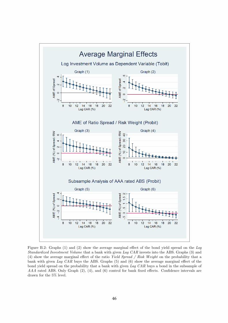
Figure B.2: Graphs (1) and (2) show the average marginal effect of the bond yield spread on the LogStandardized Investment Volume that a bank with given Lag CAR invests into the ABS. Graphs (3) and(4) show the average marginal effect of the ratio Yield Spread / Risk Weight on the probability that abank with given Lag CAR buys the ABS. Graphs (5) and (6) show the average marginal effect of thebond yield spread on the probability that a bank with given Lag CAR buys a bond in the subsample ofAAA rated ABS. Only Graph (2), (4), and (6) control for bank fixed effects. Confidence intervals aredrawn for the 5% level.

46

Figure B.3: The graph shows the RWC -specific estimates for reaching for yield. Average marginal effectsof the yield spread are estimated for different values of Lag CAR and risk weight categories with differentratings. The estimates in Graph (1) are computed using Table 3, Model I without bank fixed effects.Graph (2) is estimated using Table 3, Model II with bank fixed effects.

47

Table B.1: Yield-seeking across risk weight categories. Reported are regression coefficients andaverage marginal effects (in %) of a probit estimation. The dependent variable is 1 if the bank purchasesthe bond and zero otherwise. The specification does not control for RWC. The independent variables are:Lag CAR = capital adequacy ratio lagged by one year-quarter; Log Assets = Log(Bank Assets); Spread= bond yield spread; Nominal Maturity = nominal bond maturity; WAL = weighted average life; LogBond Size = Log(Bond Face V alue); Term Structure Level = one-month Libor rate at bond issuance;and Term Structure Slope = difference between 12-months and one-month Libor rate at bond issuance;issuance year and asset type dummies. All specifications include a constant. Standard errors are reportedin parentheses and clustered by bank. The symbols *, **, and *** represent significance levels at 10%,5%, and 1% respectively. The p-value of the Hosmer-Lemeshow goodness-of-fit test is reported for fivegroups (H0: probit correctly specified).

Coeff AMEDep. Variable: Purchase Yes/No (1) (2)

Log Assets −1.867∗∗∗ 0.262∗∗∗

(0.454) (0.095)Lag CAR −5.650 0.241

(9.139) (1.324)Spread 0.211 0.039

(0.142) (0.028)Spread × Log Assets 0.014

(0.020)Spread × Lag CAR −1.309

(0.799)

Bond Controls:Nominal Maturity −0.022∗ −0.008∗∗∗

(0.012) (0.003)WAL 0.027 −0.011∗

(0.032) (0.007)Log Bond Size 0.087 0.150∗∗∗

(0.087) (0.037)Term Structure Level −0.215∗ 0.614∗∗∗

(0.256) (0.176)Term Structure Slope 0.208 0.379∗∗∗

(0.301) (0.109)Asset Type & Issuance Year Yes Yes

Risk Weight Category RWC No No

Interactions & Fixed Effects:Bond Controls × Log Assets Yes YesBond Controls × Lag CAR Yes YesBank FE No No

N Observations 102, 239 102, 239N Banks 58 58N Bonds 1, 884 1, 884Pseudo R2 0.218 0.218Hosmer-Lemeshow GoF (p-value) 0.691 0.691

48

Table B.2: Interaction effects between yield spread, capital adequacy ratio and bank size.Reported are the interaction effects Spread × Lag CAR and Spread × Log Assets in Models I and II ofTable 3. Columns (2) and (5) report the average marginal effect (in percent) of a one percent change ofthe bond yield spread on the probability that the bank purchases the bond. The average marginal effectis reported for different values of Lag CAR and Log Assets. Standard errors of average marginal effectsare reported in parentheses. The symbols *, **, and *** represent significance levels at 10%, 5%, and 1%respectively. In Column (3), I test whether the average marginal effect of Spread is significantly smaller atcapital adequacy ratios of 0.09, 0.15 and 0.20 than at Lag CAR = 0.08. The null hypothesis is AME(LagCAR = 0.09/0.15/0.20) ≥ AME(Lag CAR = 0.08). To compute the one-sided p-values reported inColumn (3), I first compute the test statistic for an equality test, which is chi-squared distributed withone degree of freedom. It equals the square of the standard normal for which one-sided p-values can becomputed. Column (6) shows the one-sided p-values for the test whether the average marginal effect ofSpread is significantly smaller at Log Assets = 0.2, 1.6 and 2.8 than at Log Assets = 3.0.

Panel A: Interaction Effects in Model I

Spread × Lag CAR Spread × Log AssetsLag CAR (%) AME (Spread) (%) One-sided test Log Assets AME (Spread) (%) One-sided test

(1) (2) (3) (4) (5) (6)

8 0.229∗∗∗ - 0.2 0.015 0.020(0.083) (0.012)

9 0.190∗∗∗ 0.042 1.6 0.049∗ 0.026(0.063) (0.026)

15 0.079∗∗∗ 0.028 2.8 0.183∗∗ 0.040(0.029) (0.080)

20 0.017 0.019 3.0 0.227∗∗ -(0.041) (0.102)

Panel B: Interaction Effects in Model II

Spread × Lag CAR Spread × Log AssetsLag CAR (%) AME (Spread) (%) One-sided test Log Assets AME (Spread) (%) One-sided test

(1) (2) (3) (4) (5) (6)

8 1.279∗∗∗ - 0.2 0.088 0.386(0.464) (0.350)

9 0.902∗∗∗ 0.008 1.6 0.168 0.420(0.315) (0.182)

15 0.183∗∗∗ 0.007 2.8 0.239 0.428(0.049) (0.187)

20 0.021 0.004 3.0 0.254 -(0.057) (0.266)

49

Table B.3: Predicted ABS yield spread and risk weight. The table shows the predicted probabilities(in percent) that banks with Lag CARs equal to 9%, 15%, or 20% buy an ABS with a given yield spreador risk weight. The predicted probabilities are estimated with the regression coefficients of Table 3, ModelI, and are adjusted for different values of Lag CAR (lagged capital adequacy ratio), Spread (bond yieldspread), and IRB base risk weight categories. Standard errors are reported in parentheses. The symbols*, **, and *** represent significance levels at 10%, 5%, and 1%, respectively. The predicted purchaseprobabilities are then used to compute the weights of the ABS with different spreads/risk weights in theportfolio of a bank with given Lag CAR.

Panel A: Capital Adequacy Ratio = 9%

Yield Spread 16bps 30bps 35bps 50bps 60bps 85bps 115bps 150bps 220bpsPredicted prob. 0.225∗∗∗ 0.246∗∗∗ 0.254∗∗∗ 0.280∗∗∗ 0.298∗∗∗ 0.348∗∗∗ 0.419∗∗∗ 0.516∗∗∗ 0.771∗∗∗

(0.069) (0.075) (0.077) (0.083) (0.088) (0.103) (0.124) (0.157) (0.253)Weights 0.067 0.073 0.076 0.083 0.089 0.104 0.125 0.154 0.230

IRB Base RWC 12% 15% 18% 20% 35% 75% 100% 425%Predicted prob. 0.415∗∗∗ 0.403∗ 0.539 0.443∗∗ 0.119 0.052∗∗ 0.040 0.048

(0.142) (0.228) (0.534) (0.210) (0.112) (0.023) (0.029) (0.031)Weights 0.201 0.195 0.262 0.215 0.058 0.025 0.021 0.023

Panel B: Capital Adequacy Ratio = 15%

Yield Spread 16bps 30bps 35bps 50bps 60bps 85bps 115bps 150bps 220bpsPredicted prob. 0.219∗∗∗ 0.229∗∗∗ 0.233∗∗∗ 0.244∗∗∗ 0.252∗∗∗ 0.273∗∗∗ 0.300∗∗∗ 0.334∗∗∗ 0.414∗∗∗

(0.053) (0.055) (0.056) (0.058) (0.060) (0.064) (0.072) (0.082) (0.111)Weights 0.088 0.092 0.093 0.098 0.101 0.109 0.120 0.134 0.166

IRB Base RWC 12% 15% 18% 20% 35% 75% 100% 425%Predicted prob. 0.343∗∗∗ 0.177∗∗∗ 0.003 0.104∗∗ 0.040 0.066∗∗∗ 0.070 0.067

(0.089) (0.057) (0.003) (0.042) (0.040) (0.024) (0.053) (0.046)Weights 0.394 0.204 0.003 0.120 0.046 0.076 0.080 0.077

Panel C: Capital Adequacy Ratio = 20%

Yield Spread 16bps 30bps 35bps 50bps 60bps 85bps 115bps 150bps 220bpsPredicted prob. 0.272∗∗∗ 0.275∗∗∗ 0.276∗∗∗ 0.278∗∗∗ 0.280∗∗∗ 0.284∗∗∗ 0.289∗∗∗ 0.296∗∗∗ 0.309∗∗

(0.094) (0.094) (0.093) (0.093) (0.093) (0.094) (0.097) (0.102) (0.120)Weights 0.106 0.107 0.108 0.109 0.109 0.111 0.113 0.116 0.121

IRB Base RWC 12% 15% 18% 20% 35% 75% 100% 425%Predicted prob. 0.364∗∗∗ 0.110 0.000 0.037 0.022 0.109∗∗ 0.147 0.120

(0.122) (0.070) (0.000) (0.030) (0.023) (0.043) (0.121) (0.085)Weights 0.401 0.121 0.000 0.040 0.024 0.120 0.162 0.132

50

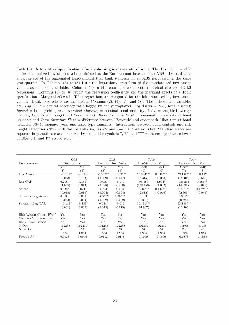
Table B.4: Alternative specifications for explaining investment volumes. The dependent variableis the standardized investment volume defined as the Euro-amount invested into ABS s by bank b asa percentage of the aggregated Euro-amount that bank b invests in all ABS purchased in the sameyear-quarter. In Columns (3) to (8) I use the logarithmic transform of the standardized investmentvolume as dependent variable. Columns (1) to (4) report the coefficients (marginal effects) of OLSregressions. Columns (5) to (8) report the regression coefficients and the marginal effects of a Tobitspecification. Marginal effects in Tobit regressions are computed for the left-truncated log investmentvolume. Bank fixed effects are included in Columns (2), (4), (7), and (8). The independent variablesare: Lag CAR = capital adequacy ratio lagged by one year-quarter; Log Assets = Log(Bank Assets);Spread = bond yield spread; Nominal Maturity = nominal bond maturity; WAL = weighted averagelife; Log Bond Size = Log(Bond Face V alue); Term Structure Level = one-month Libor rate at bondissuance; and Term Structure Slope = difference between 12-months and one-month Libor rate at bondissuance; RWC, issuance year, and asset type dummies. Interactions between bond controls and riskweight categories RWC with the variables Log Assets and Lag CAR are included. Standard errors arereported in parentheses and clustered by bank. The symbols *, **, and *** represent significance levelsat 10%, 5%, and 1% respectively.

OLS OLS Tobit TobitDep. variable: Std. Inv. Vol. Log(Std. Inv. Vol.) Log(Std. Inv. Vol.) Log(Std. Inv. Vol.)

ME ME ME ME Coeff AME Coeff AME(1) (2) (3) (4) (5) (6) (7) (8)

Log Assets −0.139∗ −0.183 -0.102∗∗ -0.127∗∗∗ -34.834∗∗∗ 0.248∗∗∗ -53.188∗∗∗ -0.157(0.083) (0.133) (0.039) (0.047) (7.315) (0.058) (12.406) (0.663)

Lag CAR 0.216 0.186 -0.023 -0.049 -95.083 -3.994∗∗ 135.253 -9.586∗∗∗

(1.045) (0.973) (0.388) (0.400) (158.456) (1.902) (340.218) (3.693)Spread 0.032∗ 0.031∗ 0.004 0.004 7.245∗∗∗ 0.144∗∗∗ 6.778∗∗∗ 0.172∗∗∗

(0.018) (0.018) (0.004) (0.004) (2.612) (0.040) (2.395) (0.044)Spread x Log Assets 0.006 0.006 0.005∗∗ 0.005∗∗ 0.469 0.901∗∗

(0.004) (0.004) (0.002) (0.002) (0.381) (0.420)Spread x Lag CAR −0.142∗ −0.135∗ -0.034∗ -0.030 -39.351∗∗∗ -53.188∗∗∗

(0.081) (0.080) (0.019) (0.019) (14.967) (12.406)

Risk Weight Categ. RWC Yes Yes Yes Yes Yes Yes Yes YesControls & Interactions Yes Yes Yes Yes Yes Yes Yes YesBank Fixed Effects No Yes No Yes No No Yes YesN Obs 102239 102239 102239 102239 102239 102239 41988 41988N Banks 58 58 58 58 58 58 23 23

1,884 1,884 1,884 1,884 1,884 1,884 1,884 1,884Pseudo R2 0.0028 0.0054 0.0102 0.0176 0.1606 0.1606 0.1878 0.1878

51

Table B.5: Purchasing ABS with a high ratio of spread over risk weight. Reported are regressioncoefficients and average marginal effects (in %) of probit estimations. The dependent variable is 1 if thebank purchases the bond and zero otherwise. The specifications do not control for the risk weights of ABSand the variable Yield Spread is replaced by the ratio Spread / Risk Weight = bond yield spread dividedby bond risk weight. The other independent variables are: Lag CAR = capital adequacy ratio lagged byone year-quarter; Log Assets = Log(Bank Assets); Nominal Maturity = nominal bond maturity; WAL= weighted average life; Log Bond Size = Log(Bond Face V alue); Term Structure Level = one-monthLibor rate at bond issuance; and Term Structure Slope = difference between 12-months and one-monthLibor rate at bond issuance; issuance year, and asset type dummies. Interactions between bond controlswith the variables Log Assets and Lag CAR are included. Bank fixed effects are controlled for in columns(3) and (4). Standard errors are reported in parentheses and clustered by bank. The symbols *, **, and*** represent significance levels at 10%, 5%, and 1% respectively.

Probit w/o bank FE Probit with bank FECoeff AME Coeff AME

Dep. Variable: Purchase Yes/No (1) (2) (3) (4)Log Assets -1.898∗∗∗ 0.261∗∗∗ -3.204∗∗∗ -0.057

(0.471) (0.094) (0.822) (1.088)Lag CAR -5.273 0.292 7.684 -7.148

(9.303) (1.336) (22.163) (5.887)Spread / Risk Weight 6.125∗∗∗ 1.720∗∗ 6.205∗∗ 4.102∗∗∗

(2.326) (0.736) (2.482) (1.457)Spread / Risk Weight x Log Assets 0.361 1.067

(0.492) (0.788)Spread / Risk Weight x Lag CAR -31.705∗∗ -42.388∗∗

(12.430) (16.825)

Risk Weight Category RWC No No No NoBond Controls & Interactions Yes Yes Yes YesBank Fixed Effects No No Yes Yes

N Obs 102239 102239 41988 41988N Banks 58 58 23 23No Bonds 1,884 1,884 1,884 1,884R2 0.2178 0.2178 0.2637 0.2637

52