Arbitrage Trading: The Long and the Short of It

Yong Chen†

Texas A&M University

Zhi Da‡

University of Notre Dame

Dayong Huang§

University of North Carolina at Greensboro

First version: December 1, 2014

This version: August 7, 2015

* We are grateful to Charles Cao, Roger Edelen, Byoung-Hyoun Hwang, Hagen Kim, Bing Liang, Jeffrey

Pontiff, Marco Rossi, Clemens Sialm, Sorin Sorescu, Zheng Sun, Jianfeng Yu, and seminar/conference

participants at Texas A&M University and the 2015 Macquarie Global Quantitative Research Conference

in Hong Kong for helpful comments. We are responsible for all remaining errors.

† Mays Business School, Texas A&M University, ychen@mays.tamu.edu.

‡ Mendoza College of Business, University of Notre Dame, zda@nd.edu.

§ Bryan School of Business, University of North Carolina at Greensboro, d_huang@uncg.edu.

Arbitrage Trading: The Long and the Short of It

August 7, 2015

Abstract

We measure arbitrage trading on both the long- and the short-sides by merging hedge fund

equity holdings with short interest. Over time, aggregate hedge fund holdings track aggregate

short interest well, and both have grown dramatically since the early 1990s. In the cross section,

net arbitrage trading, defined as the difference between abnormal hedge fund holdings and

abnormal short interest on a stock, strongly predicts future stock returns. This predictability is

not due to temporary price pressure, cannot be produced using total institutional holdings, but is

consistent with information advantage and copycat trading. When examining a broad set of

return anomalies, we find anomaly returns to come exclusively from the anomaly stocks that

are traded by arbitrageurs, and such stocks are hard to arbitrage on average. Overall, our

findings confirm that arbitrage trading is informative about mispricing.

Keywords: Hedge fund holdings, short interest, stock return anomalies, limits to arbitrage

JEL Classification: G11, G23

1

1. Introduction

Arbitrageurs play a crucial role in financial markets. By simultaneously taking long and

short positions in different assets, they help to eliminate relative mispricing and therefore enforce

market efficiency. As a result, their trading pins down the expected return on these assets,

according to the seminal Arbitrage Pricing Theory of Ross (1976). On the other hand, investors’

behavioral biases may lead to persistent mispricing when arbitrageurs face limits-to-arbitrage

(e.g., Shleifer and Vishny, 1997).

Tracking arbitrage trading has been a challenging empirical task due to the lack of data

on arbitrageurs. In recent years, as hedge funds emerge as a group of likely arbitrageurs and their

stock holdings data become available, a series of papers have inferred the long-side of arbitrage

trading by investigating their stock holdings (e.g., Brunnermeier and Nagel, 2004; Griffin and

Xu, 2009; Cao, Chen, Goetzmann, and Liang, 2014). Meanwhile, since short positions are

involved in an arbitrage trade, several studies track the short-side of arbitrage trading by

examining short interest on stocks (e.g., Hanson and Sunderam, 2014; Hwang and Liu, 2014; Wu

and Zhang, 2014).

The innovation of our paper is to combine hedge fund holdings on the long-side with

short interest on the short-side to infer net arbitrage trading on a stock. The advantage of our

approach is straightforward. A correctly priced stock can be traded by arbitrageurs for hedging

purposes, and thus some may purchase it while others sell it short. Alternatively, arbitrageurs

may disagree on the valuation of a stock, and it will be purchased in some arbitrage transactions

and sold short in others. At the end of 2012, there are more than 2,300 stocks with both hedge

fund holdings and short interest and they cover more than 90% of the U.S. equity universe in

terms of market capitalization. For these stocks, focusing on either the long- or the short-side

alone will give imprecise inference about arbitrageurs’ view on the stocks in aggregate.

However, the net position should represent a better proxy for arbitrage trading and a more

2

powerful predictor of future stock returns. Indeed, we confirm this conjecture in our empirical

analysis. In particular, we find that stocks with large hedge fund ownership and simultaneously

little short interest realize high future abnormal returns, while stock with large hedge fund

ownership but heavy short interest do not earn any abnormal return in the future.

We combine a comprehensive dataset on hedge fund stock holdings with data on short

interest during the period 1990–2012.1 Over time, aggregate hedge fund holdings track aggregate

short interest well, and both experienced exponential growth since the early 1990s. The average

percentages of shares outstanding held by hedge funds or sold short are both less than 1% in

1990 but peak around 5% in 2008 before leveling off afterwards. The common trend shared by

both the long- and the short-sides of arbitrage trading confirms the increasing arbitrage activities

documented by Hanson and Sunderam (2014) who examine short interest only. In the cross

section, we find similar distributions in hedge fund holdings and short interest. For example,

these two variables exhibit similar means (3.72% vs. 3.49%), medians (2.37% vs. 2.35%), and

standard deviations (3.97% vs. 3.66%) across stocks. The similarity in their distributions

supports the notion that on average, hedge fund holdings and short interest reveal the two legs of

the same arbitrage trade.

Stocks can be purchased by hedge funds or sold short for many reasons other than

arbitrage. For example, hedge funds may hold certain stocks to neutralize portfolio risk. Stocks

may be sold short to hedge against a convertible bond purchase. To better measure arbitrage

trading, we define abnormal hedge fund holding (AHF) and abnormal short interest (ASR) as

their values in the current quarter minus their moving averages in the prior four quarters. At the

aggregate level, AHF and ASR track each other well. This is particularly true during crisis

periods when mispricing is prevalent. Finally, AHFSR, defined as the difference between AHF

1 In our base sample, we exclude small stocks and penny stocks from our main analysis to minimize measurement

errors and market microstructure-related noise. We verify that our return results are similar when we add back small

stocks.

3

and ASR, is our net arbitrage trading measure that captures trade imbalance of arbitrageurs. For

example, an AHFSR of 1% (–1%) on a stock means that arbitrageurs, as a group, have purchased

(sold) an additional 1% of the stock during the most recent quarter relative to their past averages.

Consistent with the existing literature, we find both abnormal hedge fund holdings (AHF)

and abnormal short interest (ASR) to predict stock returns. On the long side, stocks in the highest

AHF quintile outperform those in the lowest quintile by 0.44% per month in the next quarter. On

the short side, stocks in the highest ASR quintile underperform those in the lowest quintile by

0.41% per month in the next quarter. Most importantly, by focusing on net arbitrage trading,

AHFSR generates the highest return spread in the same sample.2 Stocks in the highest AHFSR

quintile outperform those in the lowest quintile by 0.68% per month (t-value = 7.93) in the next

quarter. The return spread is highly significant but declines quickly over time. It drops to 0.42%

per month in the second quarter and further down to 0.18% per month in the third quarter. When

we extend the return horizon up to two years, we do not observe any significant spread beyond

the third quarter. In addition, the lack of return reversal in the long-run suggests that the

abnormal return spread associated with AHFSR during the first three quarters is more likely to

capture corrections to mispricing rather than temporary price pressure caused by arbitrage

trading.

The strong return predictability of our net arbitrage trading measure AHFSR holds in a

battery of robustness checks. The return predictability is not explained by the common risk

factors. Further, we obtain similar results when we restrict both hedge fund holdings and short

interest to be strictly positive (i.e., excluding zero values) and when we include small stocks in

the sample. It is strong in both the first and the second halves of the sample period. It is also

2 In a contemporaneous study, Jiao, Massa, and Zhang (2015) also find that an increase (decrease) in hedge fund

holdings accompanied with a decrease (increase) in short interest is informative about future stock return and firm

fundamental. However, they do not define AHFSR and relate it to arbitrage trading and asset pricing anomalies as

we focus on in our paper. In addition, they identify hedge funds by matching 13F institutional filings with SEC

Form ADV. Since From ADV became mandatory filings for hedge funds only in recent years, hedge funds that

became defunct before Form ADV was required cannot be identified through such matching.

4

robust to Fama-MacBeth cross-sectional regressions that control for other well-known stock

return predictors. The return predictability cannot be generated by combining total institutional

holdings and short interest. In other words, our results are not driven by the interaction between

short interest and institutional ownership previously documented by Asquith, Pathak, and Ritter

(2005) and Nagel (2005) among others. The results also confirm that abnormal hedge fund

holdings reveal the long leg of arbitrage trading much better than abnormal institutional

ownership change.

The advantage of our net arbitrage trading measure can also be illustrated by a double

sort on AHF and ASR. Holding one variable constant, sorting on the second variable still

generates a large and significant return spread, suggesting that arbitrage activities are informative

on both legs. Interestingly, we find stocks with high-AHF-high-ASR to have about the same

future returns as stocks with low-AHF-low-ASR, confirming that future returns are driven by the

net arbitrage trading. Finally and not surprisingly, stocks with high-AHF-low-ASR earn much

higher future returns than stocks with low-AHF-high-ASR (1.18% vs. 0.40% per month).

The predictive power of AHFSR for stock returns suggests that arbitrage trading is

informative about stock mispricing. Though the result is interesting on its own, we examine how

mispricing is corrected in depth. We find evidence that the correction comes from two channels.

First, a significant fraction of price correction in the first two quarters takes place during earnings

announcements when fundamental information is released to the public, which suggests an

information-related channel. Second, other types of institutional investor trade in the same

direction as the arbitrageurs subsequently, which further facilitates price convergence.

Interestingly, other institutional investors follow hedge funds’ trades with a lag of at least one

quarter, suggesting that abnormal hedge fund holdings (AHF) reveal arbitrage trading on a more

timely basis.

5

After showing that AHFSR captures net arbitrage trading well, we examine the relation

between arbitrage trading and stock anomaly returns in the cross section. We examine a total of

10 well-known stock return anomalies: book-to-market ratio of Fama and French (2008); gross

profitability of Novy-Marx (2013); operating profit of Fama and French (2015); momentum of

Jegadeesh and Titman (1993); market capitalization of Fama and French (2008); asset growth of

Cooper, Gulen, and Schill (2008), Hou, Xue, and Zhang (2014), and Fama and French (2015);

investment growth of Xing (2008); net stock issues of Fama and French (2008); accrual of Fama

and French (2008); and net operating assets of Hirshleifer, Hou, Teoh, and Zhang (2004). We

verify that the long-minus-short future return spreads averaged across these 10 anomalies are

positive and significant in our sample. The return spreads are 0.28%, 0.25%, 0.20%, and 0.15%

per month during the first, second, third, and fourth quarters, respectively.3

More importantly, anomaly returns are completely driven by the stocks in the long and

short portfolios that are traded by arbitrageurs. We define an anomaly stock to be traded by

arbitrageurs if it is in the long portfolio and recent bought by arbitrageurs (its AHFSR belongs to

the top 30%), or it is in the short portfolio and recently sold short by arbitrageurs (its AHFSR

belongs to the bottom 30%). This subset of anomaly stocks earn return spreads of 0.88%, 0.61%,

0.34%, and 0.27% per month during the first, second, third, and fourth quarters, respectively,

after portfolio formation. In sharp contrast, the rest of anomaly stocks that are not traded by

arbitrageurs do not earn any significant return spread in the next four quarters. The fact that

future abnormal returns only appear among anomaly stocks traded by arbitrageurs and these

abnormal returns decline quickly during the first year suggests that arbitrageurs are effective in

identifying mispriced stocks.

Finally, we examine stock characteristics that are related to limits to arbitrage. We find

that anomaly stocks that are not traded by arbitrageurs in general are harder to arbitrage: they

3 The magnitude is smaller compared to other studies, since we use quintile sorts instead of the more common decile

sorts and we exclude small stocks from our main analysis.

6

have higher idiosyncratic volatility and lower stock price, and are less liquid. Since they are

harder to arbitrage, they are more likely to be mispriced, consistent with the existence of future

abnormal return. In addition, the future abnormal return on anomaly stocks that are traded by

arbitrageurs, as before, comes from two channels. First, it comes from price correction following

the release of fundamental information in earnings announcements. Second, it benefits from

subsequent trades of other institutions in the same direction as arbitrageurs. Overall, our findings

confirm that mispricing arises from limits-to-arbitrage and arbitrage trading is informative about

mispricing.

Our paper contributes to a growing literature that studies hedge fund holdings and short

interest as return predictors and proxies for arbitrage activities.4 Brunnermeier and Nagel (2004)

find that hedge funds ride with the bubble during the tech bubble period. Griffin and Xu (2009)

find that changes in hedge fund ownership have only weak predictive power for future stock

returns. Griffin, Harris, Shu and Topaloglu (2011) show evidence that hedge funds destabilized

the market during the tech bubble period. On the other hand, Agarwal, Jiang, Tang, and Yang

(2013) find that hedge funds’ “confidential holdings” are informative about future stock returns.

Cao, Chen, Goetzmann, and Liang (2014) find that, compared with other institutional investors,

hedge funds tend to hold and trade undervalued stocks, and undervalued stocks with higher

hedge fund ownership realize higher future returns and are more likely to get mispricing

corrected. Reca, Sias, and Turtle (2015) also find that hedge fund demand shocks predict future

stock returns.

There is also a large body of literature that examines the information embedded in short

interest. Prior research has studied, both theoretically and empirically, the impact of short sales

on security returns. Miller (1977) argues that in the presence of heterogeneous beliefs, binding

4 There are other proxies for arbitrage trading in the literature. For example, Lou and Polk (2013) infer arbitrage

activities from the comovement of stock returns.

7

short sale constraints prevent stock prices from fully reflecting negative opinions of pessimistic

traders, leading to overpricing and low subsequent returns. Diamond and Verrecchia (1987)

show that given the high costs (e.g., no access to proceeds) of short selling, short sales are more

likely to be informative trades. Consistent with these theories, several empirical papers document

a negative association between short interest and abnormal stock returns (e.g., Asquith and

Meulbroek, 1995; Desai et al., 2002; Boehmer, Jones, and Zhang, 2008). Using institutional

ownership of stocks as a proxy for stock loan supply, Asquith, Pathak, and Ritter (2005) and

Nagel (2005) examine the impact of short sale constraints on stock returns. Asquith, Pathak, and

Ritter (2005) find that for small stocks with high short interest, low institutional ownership is

associated with more negative future returns, which confirms the effect of binding short

constraints on stock prices. However, they show that only 5% of the stocks trading on the NYSE,

AMEX, and NASDAQ have institutional ownership smaller than short interest, suggesting that

short sale constraints are not pervasive. Nagel (2005) finds that short sale constraints help

explain several cross-sectional stock return anomalies related to book-to-market ratio, analyst

forecast dispersion, turnover, and return volatility. More recently, Drechsler and Drechsler (2014)

find that short-rebate fee is an informative signal about overpricing and arbitrage trading on the

short-leg. Our net arbitrage trading measure which uses hedge fund holdings provides

incremental value than combining institutional ownership and short interest.

To the best of our knowledge, our paper is the first to combine information about

arbitrage trading on both the long- and the short-sides. Different from prior research that focuses

on either the long- or the short-side, our study provides a more complete view about the effect of

arbitrage activities. We propose a simple measure of net arbitrage trading that better predicts

future stock returns. When using the measure to study well-known return anomalies, we find

strong evidence supporting the notion that mispricing arises from limits-to-arbitrage and

arbitrage trading is informative about mispricing.

8

The rest of the paper is organized as follows. Section 2 describes our data and sample.

Section 3 examines our net arbitrage trading measure (AHFSR) as a stock return predictor.

Section 4 uses AHFSR to study stock return anomalies. Section 5 concludes.

2. Data and Sample Construction

We start our sample in 1990 as hedge fund holdings and short interest are relatively

sparse before that.5 At the end of each quarter, we exclude from our main sample stocks with

price less than $5 per share and market capitalization below the 20th percentile size breakpoint

of NYSE firms. We exclude such stocks from our main analysis for two reasons. First, hedge

funds only need to report stock positions greater than 10,000 shares or $200,000 in market value.

As a result, hedge fund holdings on small stocks and penny stocks are often underestimated.

Second, excluding these stocks helps to alleviate the associated market microstructure noise. Our

final sample still represents over 85% of the CRSP universe on average.

2.1. Hedge Fund Holdings

For the long-side, we employ the same data on hedge fund equity holdings as studied by

Cao, Chen, Goetzmann, and Liang (2014). The data are constructed by manually matching the

Thomson Reuters 13F institutional ownership database with a comprehensive list of hedge fund

company names. The hedge fund company names are collected from six hedge fund databases,

including TASS, HFR, CISDM, Bloomberg, Barclay Hedge, and Morningstar, augmented with

additional sources. Hedge funds were historically exempt from registering with the SEC as an

investment company. However, similar to other institutional investors, hedge fund management

companies with more than $100 million in assets under management are required to file quarterly

5 For example, the aggregate hedge fund holdings and short interest, as a percentage of total market capitalization of

the CRSP universe, was less than 1% on average prior to 1990.

9

reports disclosing their holdings of registered equity securities. Common stock positions greater

than 10,000 shares or $200,000 in market value are subject to disclosure. As a result, hedge fund

holdings of small stocks are likely to be neglected in the reporting, and thus excluding small

stocks from our main analysis helps to alleviate this bias. 13F filings contain long positions in

stocks, while short positions are not required to be reported.

In our study, a hedge fund is identified as a management company included in a hedge

fund database, a firm that self-identifies as a hedge fund, or a firm that imposes a threshold of

high-net-worth investors and a performance-based compensation. To address the concern that a

hedge fund manager may not appear in any hedge fund database because of the voluntary nature

of reporting to a database, a manual search is used based on a variety of online resources.

Further, following Brunnermeier and Nagel (2004) and Griffin and Xu (2009), each identified

company is manually checked to ensure that hedge fund management is its primary business

using two criteria: first, over 50% of its clients are either high-net-worth individuals or invested

in “other pooled investment vehicle (e.g., hedge funds)”, and second, the adviser is compensated

by a performance-based fee. Our final sample includes 1,517 hedge fund management firms that

collectively manage over 5,000 individual hedge funds.

The way we identify hedge fund companies has an advantage over the alternative

approach of matching 13F filings with SEC Form ADV (e.g., Jiao, Massa, and Zhang, 2015).

Since From ADV became mandatory filings for hedge funds only in recent years, hedge funds

that became defunct before Form ADV was required cannot be identified through such matching.

As a result, stock ownership of many defunct hedge funds is missing by such an approach, and

survivorship bias is likely to occur.

For each stock in our sample, we compute its quarterly hedge fund holding (HF) as the

number of shares held by all hedge funds at the end of the quarter divided by the total number of

shares outstanding. If the stock is not held by any hedge fund in that quarter, its HF is set to zero.

10

Since stocks can be held by hedge funds for reasons other than arbitrage, to better measure hedge

fund trading, we define abnormal hedge fund holding (AHF) as the current quarter HF minus the

average HF in the past four quarters. Though AHF is correlated with the change in hedge fund

holdings from the one to the next quarter, it can help to alleviate the effect of sporadic variations

in hedge fund ownership that is less likely to reveal the fund manager’s trading decisions. For

instance, when the market value of the holdings in a stock by a hedge fund fluctuates around the

disclosure requirement (i.e., $200,000) possibly due to a price change, such holdings may be

disclosed in one quarter but not in the next quarter, which creates a sporadic variations unrelated

to the fund trading. Therefore, AHF better captures the trading behavior of hedge funds.

2.2 Short Interest

Mid-month short interest is obtained from the Compustat Short Interest file from 1990 to

2012. These monthly short interest data are reported by the NYSE, AMEX, and NASDAQ. The

Compustat Short Interest file covers NASDAQ stocks only from 2003, and following the

literature, we supplement our sample with short interest data on NASDAQ prior to 2003

obtained from the exchange.

For each stock in our sample, we compute its quarterly short interest (SR) as the number

of shares sold short at the end of the quarter divided by the total number of shares outstanding. If

the stock is not covered by our short interest files, its SR is set to zero. Again, we define

abnormal short interest (ASR) as the current quarter SR minus the average SR in the past four

quarters.

11

2.3 Stock Return Anomalies

We consider 10 well-documented return anomalies largely following Fama and French

(2008) and Stambaugh, Yu and Yuan (2012), in our examination of the relation of net arbitrage

trading to anomalous stock returns.

The first anomaly is book-to-market ratio (BM) of Fama and French (1996, 2008). It is

well known that firms with higher book-to-market ratio on average have higher future returns

and these returns do not disappear after adjusting market risk using the CAPM of Sharpe (1964)

and Lintner (1965). The second anomaly is operating profit (OP) of Fama and French (2015),

who show that firms with higher operating profits have higher future returns. The third anomaly

is gross profitability (GP) of Novy-Marx (2013), who shows that firms with higher gross profit

have higher future returns. The fourth anomaly is return momentum (MOM) of Jegadeesh and

Titman (1993). In our setting, at the end of each quarter, we compute stock returns in the past 13

months by skipping the immediate month prior to the end of the quarter, divide them into

winners and losers, and hold them in the next quarter. The fifth anomaly is market capitalization

(MC) of Fama and French (1996, 2008). On average, the larger the firm size, the lower its

expected return. This size anomaly, similar to the book-to-market ratio anomaly, has a long

history, survives the CAPM risk adjustment, and has been used as a factor in the three-factor

model of Fama and French (1996), the five-factor model of Fama and French (2015), and the

four-factor model of Hou, Xue, and Zhang (2014). The sixth anomaly is asset growth (AG) of

Cooper, Gulen, and Schill (2008), Hou, Xue, and Zhang (2014), and Fama and French (2015),

who show that firms with higher growth rates of asset have lower future return. The seventh

anomaly is investment growth (IK) of Xing (2008), who shows that firms with higher investment

have lower future returns. The eighth anomaly is net stock issues (NS) examined in Ritter

(1991), Loughran and Ritter (1995), and Fama and French (2008), who find that the larger the

net stock issues, the lower the future returns. The ninth anomaly is accrual (AC) examined in

12

Sloan (1996) and Fama and French (2008), who find a negative relationship between accrual and

future stock returns. The tenth anomaly is net operating assets (NOA) of Hirshleifer, Hou, Teoh,

and Zhang (2004). They show that firms with larger operating assets have lower future returns.

We follow Fama and French (2008), Novy-Marx (2013), and Hou Xue, and Zhang

(2014) to compute book-to-market ratio, market capitalization, net stock issues, and accrual. The

calculation of gross profit follows Novy-Marx (2013). The calculation of operating profit follows

Fama and French (2015). The calculation of momentum follows Jegadeesh and Titman (1993).

The calculation of asset growth follows Cooper et al. (2008). The calculation of investment

growth follows Xing (2008). The calculation of net operating assets follows Hirshleifer et al.

(2004). For each anomaly, we construct quintile portfolios at the end of each quarter. We then

compute the monthly long-minus-short portfolio return spreads for the next quarter. Details of

the anomaly constructions are provided in the Appendix.

2.4 Sample Description

After excluding small stocks and penny stocks, our baseline sample contains about 1,600

stocks per quarter. As shown in Figure 1, the number of stocks in the sample started around

1,400 in 1990, reached a peak of 2,000 during the tech bubble, and then leveled off to 1,400

afterwards. Since only small stocks and penny stocks are excluded, our baseline sample still

covers more than 86% of the CRSP universe in terms of market capitalization.

Figure 1(a) plots the cross-sectional coverages of the hedge fund holdings (HF) data and

the short interest (SR) data over time. While most of the stocks in our sample have positive short

interest, the coverage of hedge fund holdings was relatively small at the beginning. For example,

in 1990, out of the 1,400 stocks in our sample, less than 1,000 have positive hedge fund

13

holdings.6 Nevertheless, the hedge fund holdings coverage has increased rapidly. Since 2000,

most of the stocks in our sample have both positive hedge fund holdings and short interest.

Figure 1(b) plots the percentage of market cap coverage of hedge fund holdings and short

interest. The market cap coverage is large. Stocks with positive hedge fund ownership account

for more than 90% of our baseline sample in terms of market capitalization.

Figure 2(a) plots aggregate hedge fund holdings and aggregate short interest over time.

As can be seen, aggregate hedge fund holdings and short interest track each other well. They

were both less than 1% in the early 1990s but increased to around 5% in 2008. The abnormal

hedge fund holdings (AHF) and abnormal short interest (ASR) also track each other well (with a

correlation of 0.26) as shown in Figure 2(b). AHF and ASR are particularly highly correlated

during crisis periods when mispricing is widespread. For example, their correlations exceed 60%

during the two four-year-periods surrounding the tech bubble (1999–2002) and the recent

financial crisis (2006–2009). Finally, Figure 2(c) plots the difference between hedge fund

holdings and short interest, i.e., HFSR, and the difference between abnormal hedge fund

holdings and abnormal short interest, i.e., AHFSR. Here, AHFSR can be viewed as a measure of

trade imbalance of arbitrageurs. An aggregate AHFSR of 1% (–1%) means that arbitrageurs, as a

group, have purchased (sold) an additional 1% of the market during the most recent quarter

relative to the average of the previous four quarters. We find that aggregate AHFSR fluctuates

between –0.5% and 0.5% most of the time. One exceptionally large value (below –1%) of

AHFSR occurred during late 2008 as arbitrageurs were fleeing the market due to funding

liquidity constraints.

Panel A of Table 1 summarizes the cross-sectional distributions of our main variables.

We find a similar distribution in HF and SR. For example, across stocks, they have similar

means (3.72% vs. 3.49%), medians (2.37% vs. 2.35%), and standard deviations (3.97% vs.

6 The coverage of the hedge fund holdings was even smaller prior to 1990, which is the reason we start our sample

in 1990.

14

3.66%). AHF and ASR have similar distributions as well, exhibiting similar means (0.19% vs.

0.18%), medians (0.04% vs. 0.02%), and standard deviations (1.90% vs. 1.83%). The similarity

in distributions supports the notion that HF and SR reflect the two legs of the same arbitrage

trade on average.

Panel B of Table 1 reports the cross-sectional correlations among our variables. We find

a positive correlation of 0.23 between hedge fund holdings (HF) and short interest (SR) across

stocks. In other words, a stock with high HF is also likely to have high SR. It is therefore

important to isolate net arbitrage trading on the long- and short-sides. When we examine the

correlations among AHF, ASR and AHFSR, we find AHFSR to be positively correlated with

AHF (0.64) and negatively correlated with ASR (–0.68). These correlations are far from being

perfect, suggesting that net arbitrage trading is quite different from arbitrage trading on either the

long- or the short-side.

3. Arbitrage Trading and Future Stock Returns

Since the majority of stocks are both held by hedge funds and simultaneously sold short,

we argue that net arbitrage trading between the long- and the short-side should be a more

powerful predictor of future stock returns. In this section, we test the predictive power of our

measure of net arbitrage trading (AHFSR).

3.1 Portfolio sorts

We first examine whether net arbitrage trading forecasts future stock returns using a

portfolio formation approach. As our hedge fund holdings data are at a quarterly frequency, we

form portfolios at the end of each quarter and track the portfolio returns in the following quarters.

Specifically, at the end of each quarter, we rank stocks based on their values of AHF, ASR or

15

AHFSR, and assign them into quintiles. The highest (lowest) quintile includes stocks that have

high (low) values of AHF, ASR or AHFSR. After forming the portfolios, we track excess returns

of each portfolio in the following quarters. We compute excess return of a portfolio by equally

averaging excess returns of all stocks that belong to the portfolio in that quarter. We first present

excess returns of these quintile portfolios, and then adjust risk exposures to the three factors of

Fama and French (1996), the three factors of Fama and French augmented with the Carhart

(1997) momentum factor, and the five factors of Fama and French (2015) that expand their

original three factors to include a profitability factor and an asset growth factor.

Table 2 presents results from portfolio formation. Table 2A reports results from the base

sample. Panel A shows results of the AHF quintile portfolios. The results indicate that on

average, stocks experiencing a large increase in hedge fund holding (AHF-quintile 5) have

monthly excess return of 1.05% (t-value = 2.97) in the next quarter, while stocks experiencing a

large decrease in hedge fund holdings (AHF-quintile 1) have monthly excess return of 0.61% (t-

value = 1.77). The high-minus-low AHF portfolio (AHF-HML) has monthly excess return of

0.44% (t-value = 4.98) in the next quarter. The finding is consistent with the view that hedge

fund holdings have return predictive power (e.g., Cao, Chen, Goetzmann, and Liang, 2014).

There are several reasons why our findings differ from those of Griffin and Xu (2009)

who find changes in hedge fund ownership to have only weak predictive power for future stock

returns. First, our AHF variable may capture the trading behavior of hedge funds better than a

simple change in quarterly hedge fund holdings. Second, our hedge fund coverage is more

comprehensive than that in Griffin and Xu (2009). Third, the sample period in Griffin and Xu

(2009) ends in 2004, while our sample extends to 2012. Cao, Liu, and Yu (2015) also find that

changes in hedge fund ownership significantly predict stock returns in the recent period. In Table

2E, we confirm that AHF predicts stock returns better in the second half of our sample period.

16

Panel B presents results of the ASR quintile portfolios. Stocks that experience large

increase in short interest (ASR-quintile 5) have excess return of 0.49% per month (t-value =

1.32), while stocks that experience large decrease in short interest (ASR-quintile 1) have

monthly excess return of 0.90% per month (t-value = 2.70). The high-minus-low ASR portfolio

(ASR-HML) has monthly excess return of –0.41% (t-value = –4.21). The finding confirms the

return predictive power in short interest as documented in prior research (e.g., Asquith, Pathak,

and Ritter, 2005).

Panel C combines AHF and ASR and uses AHFSR to sort the same set of stocks into

quintiles. Our results show that stocks recently bought by arbitrageurs as a group (AHFSR-

quintile 5) have monthly excess return of 1.11% with a t-value of 3.23, while stocks recently sold

by arbitrageurs as a group (AHFSR-quintile 1) have monthly excess return of 0.43% with a t-

value of 1.20. The high-minus-low AHFSR portfolio (AHFSR-HML) has monthly excess return

of 0.68% (or, about 8.16% per year) with a t-value of 7.93. Therefore, the return spread is both

economically and statistically significant.

Next, we examine alphas (i.e., risk-adjusted returns) of these quintile portfolios. The

alphas seem to be large in magnitude at extreme quintiles. This is especially true for stocks that

have high AHF and stocks that have high ASR. In particular, for the three asset pricing models

we consider, high AHF stocks have monthly alphas of 0.28% (t-value = 3.11), 0.34% (t-value =

3.92), and 0.19% (t-value = 2.12), while high ASR stocks have monthly alphas of –0.32% (t-

value = –3.09), –0.17% (t-value = –1.91), and –0.35% (t-value = –3.31), respectively. This is not

surprising, since both the hedge fund holdings variable (HF) and the short interest variable (SR)

are bounded below by zero, and thus an increase in HF or SR tends to be more informative than a

decrease.

When AHF and ASR are combined into AHFSR, alphas are large in magnitude for both

high and low AHFSR portfolios. High AHFSR stocks have monthly alphas of 0.36%, 0.42%,

17

and 0.27%, and low AHFSR stocks have monthly alphas of –0.34%, –0.22%, –0.38%,

respectively. The alphas of high-minus-low portfolios are also larger and statistically significant

for the AHFSR portfolio when comparing to those of AHF and ASR portfolios. Across the three

factor models, the monthly alphas of AHFSR-HML portfolios are 0.70%, 0.64%, and 0.65%

with t-values of 8.17, 7.57, and 7.20, compared with the alphas of AHF-HML portfolios being

0.40%, 0.38%, 0.35% with t-values of 4.50, 4.27, and 3.80, and the monthly alphas of ASR-

HML portfolios being –0.50%, –0.42%, and –0.44% with t-values of –5.42, –4.71, and –4.58,

respectively.

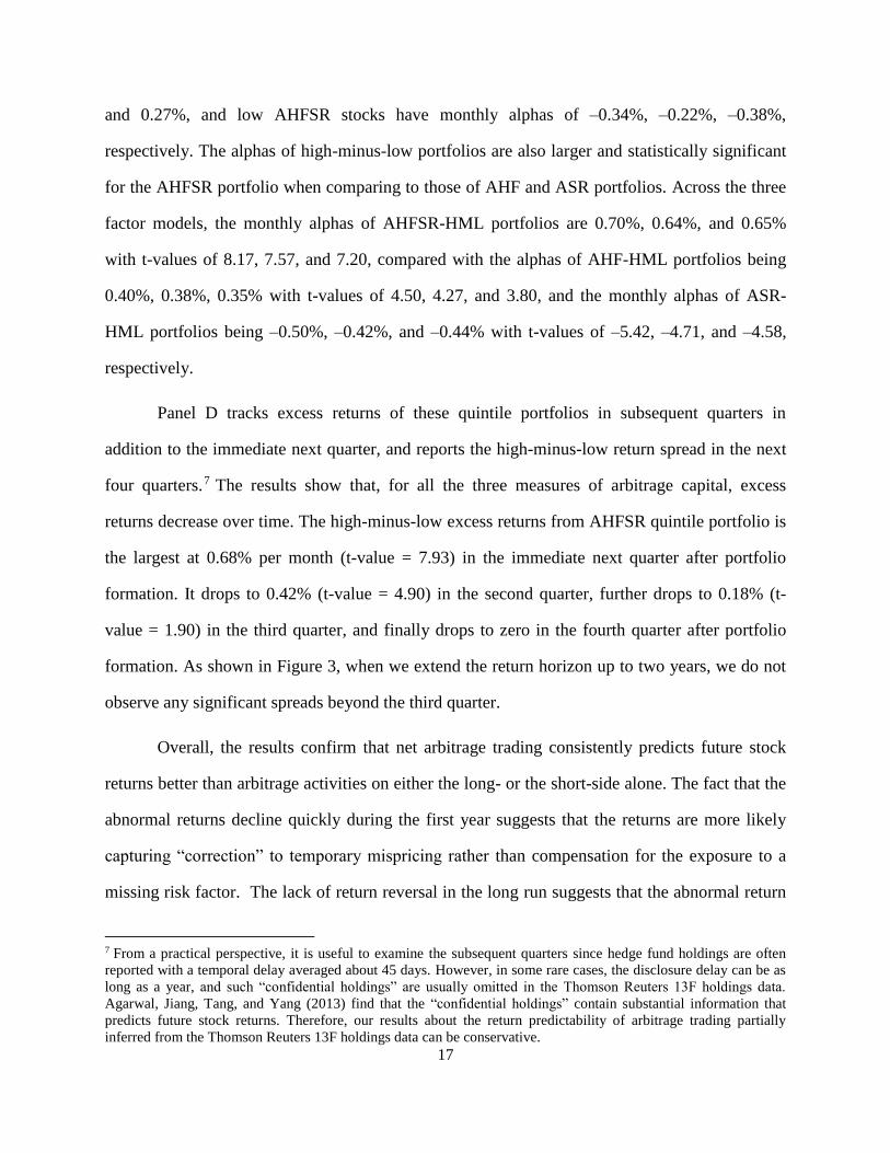
Panel D tracks excess returns of these quintile portfolios in subsequent quarters in

addition to the immediate next quarter, and reports the high-minus-low return spread in the next

four quarters.7 The results show that, for all the three measures of arbitrage capital, excess

returns decrease over time. The high-minus-low excess returns from AHFSR quintile portfolio is

the largest at 0.68% per month (t-value = 7.93) in the immediate next quarter after portfolio

formation. It drops to 0.42% (t-value = 4.90) in the second quarter, further drops to 0.18% (t-

value = 1.90) in the third quarter, and finally drops to zero in the fourth quarter after portfolio

formation. As shown in Figure 3, when we extend the return horizon up to two years, we do not

observe any significant spreads beyond the third quarter.

Overall, the results confirm that net arbitrage trading consistently predicts future stock

returns better than arbitrage activities on either the long- or the short-side alone. The fact that the

abnormal returns decline quickly during the first year suggests that the returns are more likely

capturing “correction” to temporary mispricing rather than compensation for the exposure to a

missing risk factor. The lack of return reversal in the long run suggests that the abnormal return

7 From a practical perspective, it is useful to examine the subsequent quarters since hedge fund holdings are often

reported with a temporal delay averaged about 45 days. However, in some rare cases, the disclosure delay can be as

long as a year, and such “confidential holdings” are usually omitted in the Thomson Reuters 13F holdings data.

Agarwal, Jiang, Tang, and Yang (2013) find that the “confidential holdings” contain substantial information that

predicts future stock returns. Therefore, our results about the return predictability of arbitrage trading partially

inferred from the Thomson Reuters 13F holdings data can be conservative.

18

spread associated with AHFSR is not driven by temporary price pressure caused by arbitrage

trading.

Tables 2B through 2H provide an array of robustness checks. In Table 2B, we lift the

restriction on firm size that is applied in our base sample. Specifically, we expand the base

sample with stocks whose market capitalizations are below the 20th percentile breakpoint of

NYSE firms, at the time of portfolio formation. In Table 2C, we exclude firms whose hedge fund

holdings or short interest equal to zero from the base sample. In Table 2D, we repeat our test

using the first half of the sample period covering January 1990 to June 2000, while in Table 2E,

we use the second half of the sample period covering July 2000 to December 2012. Overall, the

results from these robustness checks are similar to those presented in Table 2A. That is, our

inference is not overly sensitive to the application of size breakpoints, deletion of firms having

no hedge fund holdings or short interest, or the choice of the sample period.

So far we have assumed AHF and ASR to be comparable so that a simple difference

between them produces a measure of net arbitrage trading. The assumption seems reasonable

given that AHF and ASR have similar distributions in the cross-section (see Panel A of Table 1).

Nevertheless, to account for the possibility that true net arbitrage trading could be a nonlinear

function in both AHF and ASR, we consider an alternative approach to examine the incremental

contribution of AHF or ASR by performing two-dimensional independent sorting based on AHF

and ASR.

At the end of each quarter, we form tercile portfolios based on AHF, and independently

form tercile portfolios based on ASR. Then, nine AHF-ASR portfolios are taken from the

intersections of these two sets of tercile portfolios. Our premise is that, in the high AHF tercile,

some stocks may have high ASR, but other stocks may have low ASR. Similarly, in the low

AHF tercile, some stocks may have low ASR, but other stocks may have high ASR. However,

we posit that it is the net value that should matter. As shown in Table 2F, the average excess

19

return of stocks that have both high AHF and high ASR is 0.81% in the following quarter, while

it is 0.71% for stocks that have both low AHF and low ASR. Their corresponding alphas are both

very close to zero with small t-values, which is consistent with our expectation. In sharp contrast,

the excess returns are 1.18% for stocks that have high AHF and low ASR, and 0.40% for stocks

that have high ASR and low AHF. The corresponding risk-adjusted returns (i.e., alphas) are also

large, with the magnitude of t-values greater than 2.50 across the three factor models. Therefore,

the double-sort results provide strong support that net arbitrage trading is the driving force of the

predictability for future stock returns.

In Table 2G, we normalize both AHF and ASR by the aggregate level of institutional

holdings IO. The aggregate institutional holdings serve as a proxy for the total supply of

borrowable shares on a stock. It turns out that our results are not affected by the scaling of IO.

Finally, Table 2H reports the result of double sorting from abnormal institutional holdings (AIO)

and abnormal short interest (ASR), with AIO defined similarly to AHF. Interestingly, the result

is dramatically different from that based on AHF. The level of AIO does not predict future stock

return or alpha. Furthermore, there is no predictive power even when AIO is combined with ASR.

This suggests that hedge funds, as a likely group of arbitrageurs, are substantially different from

other types of institutions, which is consistent with the finding of Cao, Chen, Goetzmann, and

Liang (2014).

To summarize, the results suggest that some arbitrage capital buys a stock for one reason

sometimes, while other arbitrage capital sells short the same stock for another reason. Therefore,

it would be incomplete to rely on only one side of arbitrage capital to infer about arbitrageurs’

views on mispricing and future stock returns, and thus it is crucial to consider both hedge fund

holdings (the long-side) and short interest (the short-side).

20

3.2 Fama-MacBeth Cross-Sectional Regressions

As discussed in Fama and French (2008), it is difficult for the portfolio approach to

identify which variable has unique information in predicting future stock returns, because the

portfolio approach can be contaminated by choices of percentiles in the breakpoints and the order

of sorting variables. Here, we conduct Fama-MacBeth (1973) cross-sectional regressions to

further investigate the roles of AHF, ASR and AHFSR in predicting stock returns. Our sample is

quarterly at the stock level from 1990 to 2012.

The Fama-MacBeth procedure has two steps. In the first step, for each quarter, we run a

cross-sectional regression of average monthly stock excess returns over the next quarter on the

end-of-quarter AHF, ASR, or AHFSR, along with control variables. The control variables are

other return predictors identified in the existing literature, including book-to-market ratio of

Fama and French (2008); gross profitability of Novy-Marx (2013); operating profit of Fama and

French (2015); momentum of Jegadeesh and Titman (1993); market capitalization of Fama and

French (2008); asset growth of Cooper, Gulen, and Schill (2008), Hou, Xue, and Zhang (2014),

and Fama and French (2015); investment growth of Xing (2008); net stock issues of Fama and

French (2008); accrual of Fama and French (2008); and net operating assets of Hirshleifer, Hou,

Teoh, and Zhang (2004). In constructing the control variables, monthly stock returns are

obtained from the CRSP. Annual accounting data used for calculating the control variables are

from COMPUSTAT. These characteristics of each firm from the third quarter of year t to the

second quarter of year t+1 are based on its accounting information of the last fiscal year that ends

in calendar year t-1. All explanatory variables are winsorized at the 1% and 99% levels, and

standardized at the end of each quarter. Next, in the second step, we average the regression

coefficient estimates over the quarters and compute their t-values based on Newey and West

(1987) standard errors with four lags.

21

Table 3 reports the results from Fama-MacBeth regressions. Panel A presents results

from the base sample. The regression coefficients on AHF, ASR, and AHFSR are all significant

and have expected signs, even after controlling for other stock return predictors. The coefficient

on AHF is 0.15% (t-value = 5.39), while the coefficient on ASR is -0.14% (t-value = –4.10). The

coefficient on AHFSR is 0.22% (t-value = 5.82). Thus, if AHFSR increases by one standard

deviation in the current quarter, the stock excess return would rise by 0.22% per month in the

next quarter. Again, combing information in AHF and ASR leads to greater forecasting power

for future stock returns.

Next, we repeat the test by restricting our sample to only stocks that have positive hedge

fund holdings and short interest, and breaking the sample period into two equal subperiods. As

presented in Panels B–D of Table 3, our main results hold in these sensitivity tests.

A number of control variables are included in the Fama-MacBeth regressions. Overall,

regression coefficients on the control variables have correct signs, but many of these control

variables are statistically insignificant. Apart from the NYSE size filter and $5 price filter we

apply, a possible explanation is that these anomalies compete with each other and render each

other insignificant. For example, AG competes with IK, and OP competes with GP, though each

of these variables by themselves can be significant. The other possible explanation is the sample

period we use. In our sample from 1990 to 2012, the value spread (from Kenneth French’s

website) is small at 0.25% per month. During the period, momentum trading suffers from a crash

in the first half of 2009. In fact, momentum is highly significant in the first half of our sample

period (see Panel C) but insignificant in the second half of the sample period (see Panel D).

Combined, momentum is insignificant in predicting future excess returns in our sample.

Intriguingly, net operating asset is significant in our base sample. Nevertheless, further check

reveals that it is only significant in the first half of the sample period.

22

In sum, by performing Fama-MacBeth regressions, we show that net arbitrage trading as

proxied by AHFSR has stronger predictive power for future stock returns than either the long- or

the short-side does. The predictability of AHFSR is over and above that of many other firm-level

variables that can potentially forecast stock returns as well.

3.3 Sources of the Arbitrage Profits

Our results suggest that net arbitrage trading is informative about stock mispricing and

associated with future abnormal returns for at least two quarters. This predictive power for stock

returns can arise from at least two channels. First, arbitrageurs possess and trade on private

information about the fundamental value of a stock. The information is later released to the

market through earnings announcement or other information dissemination channels. Under this

information channel, we would expect the abnormal returns associated with AHFSR to occur

during future information announcement events. Second, arbitrage trading, after its disclosure,

attracts the attention of other traders. Then, the initial arbitrage trades and subsequent copycat

trading in the same direction together move stock prices closer to fundamental values.8 Under the

copycat trading channel, we would expect AHFSR in quarter t to predict trading by other

institutional investors in the near future.

Table 4 examines both the channels. Panel A reports the average stock return around

earnings announcements (in a five-day window) across the AHFSR-sorted quintiles. The stocks

purchased by arbitrageurs in quarter t (high-AHFSR) outperform those sold by arbitrageurs (low-

AHFSR) by 0.14% (t-value = 4.72) during the earnings-announcement window in quarter t+1,

and another 0.10% (t-value = 3.43) in quarter t+2. Thus, the evidence supports the private

information channel.

8 Brown and Schwarz (2013) show evidence of copycat trading after the disclosure of hedge fund holdings. In

particular, they find abnormal trading volume and positive returns immediately after the disclosure.

23

Panel B of Table 4 reports, for each of the AHFSR-sorted quintile portfolios, the average

changes in institutional ownership (excluding hedge fund ownership) from quarter t to t+1, t+2,

t+3, and t+4, respectively. Consistent with the rise in equity ownership by institutions during our

sample period, the average change in institutional ownership is always positive. Nevertheless,

the change is monotonically increasing in AHFSR. The differences in institutional ownership

change between the high- and the low-AHFSR quintiles are significant for up to a year. In other

words, net arbitrage purchase in quarter t strongly predicts the purchase by other institutions in

the next year. Hence, the evidence supports the copycat trading channel. To have a complete

picture, we also look at changes in non-hedge fund holdings (CNHF) in the current quarter t.

Interestingly, non-hedge funds appear to trade in the opposite direction to the arbitrage force. In

particular, stocks with highest (lowest) AHFSR actually experience selling (buying) from non-

hedge funds as a whole in the current quarter. This result confirms the importance to separate

hedge funds from other institutions.

To summarize, arbitrage trading is informative about stock mispricing and the mispricing

is corrected through two channels. First, stock prices move closer to fundamentals as the private

information is released to the public. Second, other institutions trade in the same direction as the

arbitrageurs subsequently, which further facilitates price convergence.

4. Arbitrage Trading and Stock Return Anomalies

As AHFSR measures net arbitrage trading, we now use it to shed light on how

arbitrageurs trade on well-known return anomalies. As detailed in Section 2.3, we examine a

total of 10 anomalies, namely book-to-market ratio, gross profitability, operating profit,

momentum, market capitalization, asset growth, investment-to-capital ratio, net stock issues,

accrual, and net operating assets.

24

Panel A of Table 5A verifies that the long-minus-short future return spreads averaged

across these 10 anomalies are positive and significant in our sample. The average monthly return

spreads are 0.28% (t-value = 3.47), 0.25% (t-value = 3.19), 0.20% (t-value = 2.48), and 0.15% (t-

value = 1.97) per month during the first, second, third, and fourth quarters, respectively. The

magnitude is somewhat smaller compared with previous studies, since we use quintile sorts

instead of the more common decile sorts and we exclude small stocks from our main sample. As

discussed above, the sample period is likely to play a role as well, and several anomalies have

smaller returns during the recent period. Not surprisingly, when we control for return factors

constructed on some of the anomalies, the resulting average five-factor alphas become smaller.

They are 0.14% (t-value = 2.27), 0.13% (t-value = 1.99), 0.11% (t-value = 1.46), and 0.08% (t-

value = 1.18) per month during the first, second, third, and fourth quarters, respectively. The

average alphas are still significant during the first two quarters after portfolio formation, as

shown in Panel A of Table 5B. In addition, consistent with the findings of Stambaugh, Yu, and

Yuan (2012), most of the anomaly alphas come from the short leg since overpricing is harder to

arbitrage due to short-sale constraints.

We then identify stocks in the long- and short-anomaly portfolios that are traded by

arbitrageurs in the same direction. We classify an anomaly stock to be traded by arbitrageurs if it

is in the long portfolio and recently bought by arbitrageurs (its AHFSR belongs to the top 30%),

or it is in the short portfolio and recently sold short (its AHFSR belongs to the bottom 30%).9

Table 5C shows that these stocks account for about 30% of both the long- and the short-

portfolios. Strikingly, the anomaly returns are completely driven by these stocks that are traded

by arbitrageurs. As shown in Panel B of Table 5A, this subset of anomaly stocks earn return

spreads of 0.88% (t-value = 7.10), 0.61% (t-value = 4.88), 0.34% (t-value = 2.68), and 0.27% (t-

value = 2.18) per month during the first, second, third, and fourth quarters, respectively. The

9 Alternatively, we consider a less restrictive classification. Specifically, we classify an anomaly stock to be traded

by arbitrageurs if it is in the long portfolio with a positive AHFSR, or it is in the short portfolio with a negative

AHFSR. We find the same result that anomaly returns only come from anomaly stocks traded by arbitrageurs.

25

corresponding five-factor alphas are 0.70% (t-value = 6.31), 0.45% (t-value = 3.90), 0.25% (t-

value = 1.98), and 0.22% (t-value = 1.73). Hence, the alpha shows a quick decline over time

during the first year.10 When we examine the alphas on the long- and short-legs separately, we

again find the alphas to come mostly from the short-leg. While the alpha on the long-leg is small

and significant only in the first quarter, the alpha more than doubles on the short-leg and persists

for a longer time.

In sharp contrast, the other 70% of anomaly stocks that are not traded by arbitrageurs do

not earn any significant return spreads or alphas in any of the next four quarters, as reported in

Panel C of Table 5A. This is true for both the long- and the short-legs. The fact that future

abnormal returns only appear among anomaly stocks traded by arbitrageurs and these abnormal

returns decline quickly during the first year suggests that arbitrage trading is informative about

the mispricing. A close examination of Tables 5A and 5B confirms that our findings are not

driven by one or two anomalies. Instead, the pattern appears consistently and uniformly across

the 10 return anomalies.

So far, our findings suggest that anomaly stocks are not created equal. Only the anomaly

stocks traded by arbitrageurs seem to be mispriced. A natural question follows: How do anomaly

stocks that are traded by arbitrageurs differ from those that are not traded? We compare these

two subsets of anomaly stocks by examining their stock price, idiosyncratic volatility, and the

Amihud (2002) illiquidity measure at the portfolio level. The Amihud measure is transformed

into percentiles among NYSE/AMEX or NASDAQ firms separately.

Table 6 reports results of the comparisons. Across almost all the anomalies and for both

the long- and the short-portfolios, anomaly stocks that are traded have significantly lower prices

and higher idiosyncratic volatilities and are also significantly less liquid according to the Amihud

measure. Pontiff (1996) and Shleifer and Vishny (1997) argue that idiosyncratic volatility is a

10 Akbas, Armstrong, Sorescu, and Subrahmanyam (2014) find that aggregate money flow into the hedge fund

industry attenuates stock return anomalies.

26

major arbitrage cost. In addition, it is well known that hedge funds often hold illiquidity assets

(e.g., Getmansky, Lo, and Marakov, 2004). Thus, the evidence is consistent with a notion that

anomaly stocks are harder to arbitrage, explaining why they are mispriced to start with.

Table 6 also reports the difference in the anomaly characteristic variable (standardized by

its cross-sectional deviation) between anomaly stocks traded by arbitragers and those not traded.

While it is true that stocks traded by arbitrageurs in general are associated with more extreme

anomaly characteristic, the difference in the anomaly characteristic is too small to explain the

future return difference. For example, among all value stocks, the ones bought by arbitrageurs

have a book-to-market ratio only 1% higher (relative to the cross-sectional deviation in BM) than

the remaining value stocks. Among all growth stocks, the ones sold by arbitrageurs have a book-

to-market ratio that is only 5% lower than the remaining growth stocks. These small differences

in book-to-market ratio are unlikely to explain the much higher return spread in the next quarter

(0.76% per month as reported in Panel D of Table 5A) on the value anomaly traded by

arbitrageurs.

Finally, Table 7 examines future earnings-announcement-window returns and non-hedge-

fund institutional trading of the long- and the short-portfolios. Consistent with the earlier

findings in Table 4, the abnormal returns on anomaly stocks traded by arbitrageurs come from

two channels. First, as the private information is released to the public, prices move closer to

fundamentals. Second, other institutions trade in the same direction as the arbitrageurs

subsequently, further facilitating price convergence for the anomaly stocks. Interestingly, among

the anomaly stocks not traded by arbitrageurs, other institutions actually purchase more

overpriced stocks (short-portfolio) than underpriced stocks (long-portfolio) subsequently despite

the fact the underprice stocks indeed experience higher earnings-announcement-window returns

during quarters t+3 and t+4 (but not in the first two quarters). Finally, similarly to the result in

27

Table 4, other institutions appear to trade in the opposite direction as the arbitrage force in the

current quarter.11

Taken together, we find that net arbitrage trading contains useful prospective information

about stock returns. Furthermore, anomaly stocks have large arbitrage costs, and their anomalous

returns are significantly associated with net arbitrage trading. These findings confirm that

mispricing is related to limits-to-arbitrage and arbitrage trading is informative about mispricing.

5. Conclusion

Arbitrageurs play a crucial role in finance, but measuring their activities has been a

challenge task empirically. By merging hedge fund stock holdings with short interest on stocks,

we track arbitrage trading on both the long- and the short-sides. Over time, aggregate hedge fund

holdings track aggregate short interest well, and both experienced fast growth since the early

1990s. In the cross section, net arbitrage trading, defined as the difference between abnormal

hedge fund holdings and abnormal short interest on a stock, strongly predicts future stock returns.

When examining a broad set of stock return anomalies, we find anomaly returns to come

exclusively from the anomaly stocks that are traded by arbitrageurs. These stocks are also hard to

arbitrage on average. Overall, our findings confirm that mispricing is related to limits-to-

arbitrage and arbitrage trading is informative about mispricing.

Our simple measure of arbitrage trading can be used in many other applications. For

example, one could relate arbitrage trading on an anomaly to its future performance. It would

also be interesting to use the return spread between stocks with high- and low-AHFSR as a

pricing factor in the spirit of the APT. We leave these topics for future research.

11 Edelen, Ince, and Kadlec (2014) also find that institutional trades tend to be on the wrong side in that institutional

investors increase their ownership for overvalued stocks and decrease their ownership for undervalued stocks.

However, they do not study hedge funds separately relative to other types of institutional investors.

28

Appendix: Details of the Constructions of Stock Return Anomalies.

This appendix provides the details of the constructions of the 10 stock return anomalies

we examine in the paper. Following the convention in Fama and French (2008), Novy-Marx

(2013), and Hou, Xue, and Zhang (2014), the financial/accounting ratios for each stock from July

of year t to June of year t+1 (third quarter of year t to second quarter of year t+1) is its financial

ratios for the last fiscal year ending in calendar year t-1. At the end of each quarter, we sort all

stocks into quintiles based on their financial ratios. Monthly excess returns in the next three

months are calculated as equal-weighted averages of excess returns of individual firms in each

portfolio. The portfolio is rebalanced each quarter at the end of March, June, September, and

December.

1. Book-to-market ratio (BM). Book equity is stockholders’ book equity, plus balance sheet

deferred taxes (Compustat item ITCB) and investment tax credit (TXDB) if available,

minus the book value of preferred stock. We employ tiered definitions largely consistent

with those used by Davis, Fama, and French (2000), Novy-Marx (2013) and Hou, Xue,

and Zhang (2014) to construct stockholders’ equity and book value of preferred stock.

Stockholders equity is as given in Compustat (SEQ) if available, or else common equity

(CEQ) plus the book value of preferred stock, or else total assets minus total liabilities

(AT–LT). Book value of preferred stock is redemption value (PSTKRV) if available, or

else liquidating value (PSTKL) if available, or else par value (PSTK). Book-to-market

ratio in year t-1 is computed as book equity for the fiscal year ending in calendar year t-1

divided by the market capitalization at the end of December of t-1. Stocks with missing

book values or negative book-values are deleted.

2. Gross Profit to Asset (GP). Following Novy-Marx (2013), we measure gross profits-to-

assets in year t-1 as gross profit in year t-1 (Compustat item GP) divided by total assets in

year t-1 (AT).

29

3. Operating Profit (OP). Following Fama and French (2015), we measure operating profit

in year t-1 as year t-1 gross profit (Compustat item GP), minus selling, general, and

administrative expenses (XSGA) if available, minus interest expense (XINT) if available,

all divided by year t-1 book equity. Stocks with missing book value or negative book-

value are deleted.

4. Momentum (MOM). Similar to Jegadeesh and Titman (1993), at the end of March, June,

September, and December (month t), we compute each stock’s cumulative return from

month t-13 to t-2, and form quintile portfolios for the next three months. We compute

equal-weighted monthly returns in each portfolio for month t+1 to t+3, and the portfolio

is rebalanced at the end of month t+3.

5. Market Capitalization (MC). Following Fama and French (2008), MC is defined as the

market capitalization at the end of June in each year. It is the product of number of shares

and shares outstanding from the CRSP. This MC is used for the following four quarters.

6. Asset Growth (AG). Following Cooper, Gulen, and Schill (2008), we compute asset

growth in year t-1 as total assets (AT) for the fiscal year ending in calendar year t-1

divided by total assets for the fiscal year ending in calendar year t-2, minus one.

7. Investment growth (IK). Following Xing (2008), we measure investment growth for year

t-1 as the growth rate in capital expenditure (CAPX) from the fiscal year ending in

calendar year t-2 to the fiscal year ending in t-1.

8. Net stock issues (NS). Following Fama and French (2008), we compute net stock issues

in year t-1, as the split-adjusted shares outstanding for fiscal year ending in calendar year

t-1 divided by the split-adjusted shares outstanding for fiscal year ending in calendar year

t-2, minus one. The split-adjusted shares outstanding are calculated as shares outstanding

(CSHO) times the adjustment factor (AJEX).

9. Accrual (AC). Accruals in year t-1 are defined following Fama and French (2008), as the

change in operating working capital per split-adjusted share from t-2 to t-1 divided by

30

book equity per split-adjusted share at t-1. Operating working capital is computed as

current assets (ACT) minus cash and short-term investments (CHE), minus the difference

of current liability (LCT) and debt in current liabilities (DLC) if available.

10. Net Operating Assets (NOA). Following Hirshleifer et al. (2004), we define net operating

assets (NOA) in year t-1, as operating assets minus operating liabilities in year t-1 scaled

by total assets in year t-2 (Compustat item AT). Operating assets are total assets (AT)

minus cash and short-term investment (CHE). Operating liabilities are total assets minus

debt included in current liabilities (item DLC, zero if missing), minus long-term debt

(item DLTT, zero if missing), minus minority interests (item MIB, zero if missing),

minus book value of preferred stocks as described in the definition of book equity (zero if

missing), and minus common equity (CEQ).

31

References

Agarwal, Vikas, Wei Jiang, Yuehua Tang, and Baozhong Yang, 2013, Uncovering hedge fund

skill from the portfolio holdings they hide, Journal of Finance 59, 1271–1289.

Akbas, Ferhat, William Armstrong, Sorin Sorescu, and Avanidhar Subrahmanyam, 2014, Smart

money, dumb money, and equity return anomalies, Journal of Financial Economics, forthcoming.

Amihud, Yakov, 2002, Illiquidity and stock returns: cross section and time series effects, Journal

of Financial Markets 5, 31–56.

Asquith, P., and L. Meulbroek, 1995. An empirical investigation of short interest, Working paper,

M.I.T.

Asquith, Paul, Parag Pathak, and Jay Ritter, 2005, Short Interest, Institutional Ownership, and

Stock Returns, Journal of Financial Economics 78, 243–276.

Boehmer, Ekkehart, Charles Jones, and Xiaoyan Zhang, 2008, Which Shorts are Informed?

Journal of Finance 63, 491–527.

Brown, Stephen, and Christopher Schwarz, 2013, Does market participants care about portfolio

disclosure? Evidence from hedge fund 13F filings, Working paper, NYU and UC Irvine.

Brunnermeier, Markus, and Stefan Nagel, 2004, Hedge funds and the technology bubble,

Journal of Finance 59, 2013–2040.

Cao, Charles, Yong Chen, William Goetzmann, and Bing Liang, 2014, The role of hedge fund in

the security price formation process, Working paper.

Cao, Charles, Clark Liu, and Jianfeng Yu, 2015, Smart money or dumb money? Working paper.

Carhart, Mark, 1997, On persistence in mutual fund performance, Journal of Finance 52, 57–82.

Cooper, Michael, Huseyin Gulen, and Michael Schill, 2008, Asset growth and the cross-section

of stock returns, Journal of Finance 63, 1609–52.

Davis, James, Eugene Fama, and Kenneth French, 2000, Characteristics, covariances, and

average returns: 1929 to 1997, Journal of Finance 55, 389–406.

Desai, H., K. Ramesh, S. R. Thiagarajan, and B. V. Balachandran, 2002, An Investigation of the

Informational Role of Short Interest in the Nasdaq Market, Journal of Finance 57, 2263–2287.

Diamond, Douglas, and Robert Verrecchia, 1987, Constraints on short-selling and asset price

adjustment to private information, Journal of Financial Economics 18, 277–311.

32

Drechsler, Itamar, and Qingyi Drechsler, 2014, Theshorting premium and asset pricing

anomalies, Working paper, New York University.

Edelen, Roger, Ozgur Ince, and Gregory Kadlec, 2014, Institutional investors and stock return

anomalies, Working paper, UC Davis and Virginia Tech.

Fama, Eugene, and Kenneth French, 1996, Multifactor explanations of asset pricing anomalies,

Journal of Finance 51, 55–87.

Fama, Eugene, and Kenneth French, 2008, Dissecting anomalies, Journal of Finance 63, 1653–

1678.

Fama, Eugene, and Kenneth French, 2014, A five-factor asset pricing model, Journal of

Financial Economics, forthcoming.

Fama, Eugene, and James MacBeth, 1973, Risk, return, and equilibrium–empirical tests, Journal

of Political Economy 81, 607–636.

Getmansky, M., Lo, A. W., Makarov, I., 2004, An econometric model of serial correlation and

illiquidity in hedge fund returns, Journal of Financial Economics 74, 529–609.

Griffin, John, Jeffrey Harris, Tao Shu, and Selim Topaloglu, 2011, Who drove and burst the tech

bubble?, Journal of Finance 66, 1251–1290.

Griffin, John, and Jin Xu, 2009, How smart are the smart guys? A unique view from hedge fund

stock holdings, Review of Financial Studies 22, 2531–2570.

Hanson, Samuel, and Adi Sunderam, 2014, The Growth and Limits of Arbitrage: Evidence from

Short Interest, Review of Financial Studies 27, 1238–1286.

Hirshleifer, David, Kewei Hou, Siew Hong Teoh, and Yinglei Zhang, 2004, Do investors

overvalue firms with bloated balance sheets, Journal of Accounting and Economics 38, 297–331.

Hou, Kewei, Chen Xue, and Lu Zhang, 2014, Digesting anomalies: An investment approach,

Review of Financial Studies, forthcoming.

Hwang, Byoung-Hyoun, and Baixiao Liu, 2014, Short sellers’ trading anomalies, Working paper,

Cornell University.

Jegadeesh, N., and S. Titman, 1993, Returns to buying winners and selling losers: Implications

for stock market efficiency, Journal of Finance 48, 65–91.

Jiao, Y., M. Massa, and H. Zhang, 2015, Short selling meets hedge fund 13F: An anatomy of

informed demand, Working paper, INSEAD.

33

Lintner, John, 1965, The valuation of risk assets and the selection of risky investments in stock

portfolios and capital budgets, Review of Economics and Statistics 47, 13–37.

Lou, Dong, and Christopher Polk, 2014, Comomentum: Inferring Arbitrage Activity from Return

Correlations, Working paper, London School of Economics.

Loughran, T., and J. R. Ritter, 1995, The New Issues Puzzle, Journal of Finance 50, 23–51.

Miller, E., 1977, Risk, uncertainty, and divergence of opinion, Journal of Finance 32, 1151–

1168.

Nagel, Stefan, 2005, Short sales, institutional ownership, and the cross-section of stock returns,

Journal of Financial Economics 78, 277–309.

Newey, W.K., and K. D. West, 1987, A simple, positive definite, heteroskedasticity and

autocorrelation consistent covariance matrix, Econometrica 55, 703–708.

Novy-Marx, Robert, 2013, The other side of value: The gross profitability premium. Journal of

Financial Economics 108, 1–28.

Pontiff, Jeffrey, 1996, Costly arbitrage: Evidence from closed-end funds, Quarterly Journal of

Economics 111, 1135–1151.

Reca, Blerina B., Richard W. Sias, and Harry J. Turtle, 2015, Hedge fund crowds and mispricing,

Management Science, forthcoming.

Ritter, Jay, 1991, The long-run performance of initial public offerings, Journal of Finance 46, 3–

27.

Ross, Stephen, 1976, The arbitrage theory of capital asset pricing, Journal of Economic Theory

13, 341–360.

Sharpe, William F., 1964, Capital asset prices: A theory of market equilibrium under conditions

of risk, Journal of Finance 19, 425–442.

Shleifer, Andrei, and Robert Vishny, 1997, The limits of arbitrage, Journal of Finance 52, 35–55.

Sloan, R., 1996, Do stock prices fully reflect information in accruals and cash flows about future

earnings? The Accounting Review 71, 289–315.

Stambaugh, Robert, Jianfeng Yu, and Yu Yuan, 2012, The short of it: Investor sentiment and

anomalies, Journal of Financial Economics 104, 288–302.

Wu, Julie, and Andrew Zhang, 2014, Have short sellers become more sophisticated? Evidence

from market anomalies, Working paper, University of Georgia.

34

Xing, Yuhang, 2008, Interpreting the value effect through the Q-theory: An empirical

investigation, Review of Financial Studies 21, 1767–1795.

35

Table 1. Summary Statistics

This table presents summary statistics for the following variables: hedge fund holdings (HF), defined as the ratio between shares owned by hedge

funds and the number of outstanding shares; short interest (SR), defined as the ratio between shares shorted and the number of shares outstanding;

the difference between HF and SR (HFSR); abnormal hedge fund holdings (AHF), defined as the percentage change of current HF from the

average HF in the previous four quarters; abnormal short ratio (ASR), defined as the percentage change of current SR from the average SR in the

previous four quarters; and the difference between AHF and ASR (AHFSR). Panel A reports the summary statistics including the mean, 5th

percentile, 25th percentile, median, 75th percentile, 95th percentile, and standard deviation. At the end of each quarter, we first compute the

variables across stocks, and then take average across quarters. % of CRSP represents the total market capitalization of our sample stocks as a

fraction of the market capitalization of the full CRSP universe. In each quarter, we delete firms with market capitalizations below the 20th

percentile size breakpoint of NYSE firms. Panel B presents average correlations between HF, SR, HFSR, AHF, ASR, AHFSR and stock

characteristics over quarters. We consider the following stock characteristics: book-to-market ratio (BM) of Fama and French (2008); gross

profitability (GP) of Novy-Marx (2013); operating profit (OP) of Fama and French (2015); momentum (MOM) of Jegadeesh and Titman (1993);

market capitalization (MC) of Fama and French (2008); asset growth (AG) of Cooper, Gulen, and Schill (2008), Hou, Xue, and Zhang (2014), and

Fama and French (2015); investment-to-capital ratio (IK) of Xing (2008); net stock issues (NS) of Fama and French (2008); accrual (AC) of Fama

and French (2008); and net operating assets (NOA) of Hirshleifer, Hou, Teoh, and Zhang (2004). Monthly stock returns are from the CRSP.

Annual accounting data used for calculating the stock characteristics are from COMPUSTAT. The characteristics of each firm from July of year t

to June of year t+1 are based on its accounting information of the last fiscal year that ends in calendar year t-1. The sample period is from 1990Q1

to 2012Q4.

36

Table 1, continued.

Panel A: Summary (in percentage)

Mean P5 P25 P50 P75 P95 STD

HF 3.72 0.34 1.12 2.37 4.90 12.01 3.97

SR 3.49 0.38 1.12 2.35 4.44 11.20 3.66

HFSR 0.23 -7.42 -1.63 0.13 1.88 8.23 4.69

AHF 0.19 -2.67 -0.55 0.04 0.75 3.63 1.90

ASR 0.18 -2.37 -0.52 0.02 0.69 3.38 1.83

AHFSR 0.00 -4.50 -1.03 0.02 1.06 4.45 2.66

% of CRSP 86.73 74.87 85.50 87.29 89.26 92.22 4.50

Panel B: Correlation

HF SR HFSR AHF ASR AHFSR BM GP OP MOM MC AG IK NS AC NOA

HF 1.00 0.23 0.63 0.42 0.06 0.24 0.00 0.06 -0.04 0.06 -0.17 0.08 0.06 0.08 -0.01 0.06

SR 0.23 1.00 -0.59 0.04 0.45 -0.30 -0.09 0.08 -0.08 -0.04 -0.20 0.19 0.11 0.11 0.05 0.10

HFSR 0.63 -0.59 1.00 0.30 -0.31 0.45 0.08 -0.02 0.03 0.07 0.00 -0.09 -0.04 -0.02 -0.05 -0.03

AHF 0.42 0.04 0.30 1.00 0.07 0.64 0.01 0.01 -0.01 0.02 -0.03 -0.02 0.00 -0.02 -0.01 -0.01

ASR 0.06 0.45 -0.31 0.07 1.00 -0.68 -0.03 0.01 -0.02 -0.02 -0.05 0.05 0.03 0.02 0.02 0.02

AHFSR 0.24 -0.30 0.45 0.64 -0.68 1.00 0.03 0.00 0.01 0.02 0.01 -0.04 -0.03 -0.03 -0.02 -0.02

37

Table 2. Stock Returns and Alphas of Portfolios Formed on Arbitrage Capital

At the end of each quarter, we form quintile portfolios based on AHF, ASR, or AHFSR, and track each portfolio’s monthly excess returns in the

next quarter, which are the equal-weighted average of excess returns on stocks in each portfolio. Quintile 5 has the highest AHF, ASR or AHFSR.

We adjust risk exposures using the three factors of Fama and French (1996), the Fama-French three factors and the Carhart (1997) momentum

factor, and the five factors of Fama and French (2015) that are labelled as FF3, FF4, and FF5, respectively. Panel A presents results for the

portfolios formed on AHF, Panel B presents results for the portfolios formed on ASR, Panel C presents results for the portfolios formed on

AHFSR, and Panel D presents return spreads of these portfolios in the next four quarters. The left panels present excess returns and alphas, and the

right panels report their t-values. Table 2A uses our base sample that deletes the firms with market capitalizations below the NYSE 20th percentile

size breakpoint. Table 2B presents results from using a sample without applying the firm size filter. Table 2C uses firms that have strictly positive

HF and SR in our base sample. Table 2D uses the first half of the sample period. Table 2E uses the second half of the sample period. Table 2F

presents results from tercile portfolios independently formed on AHF and ASR in our base sample. Stock excess return and alpha are reported in

percent per month. Table 2G (Panel A) repeats the quintile AHFSR sorting but with HF and SR scaled by total institutional ownership. The

variable AHFSRIO represents the AHFSR constructed using scaled HF and SR. Table 2G (Panel B) presents next four quarters returns for

AHFSRIO sorting. Table 2H, similar to table 2F, presents double sorting result from AIO and ASR, where AIO is abnormal IO defined similarly

to abnormal HF or abnormal SR. Panel A through D in table 2H presents next quarter returns and various alphas and their t-values. Panel E in

table 2H presents the next four quarter returns of portfolios formed on AIO and ASR. The sample period is from 1990Q1 to 2012Q4.

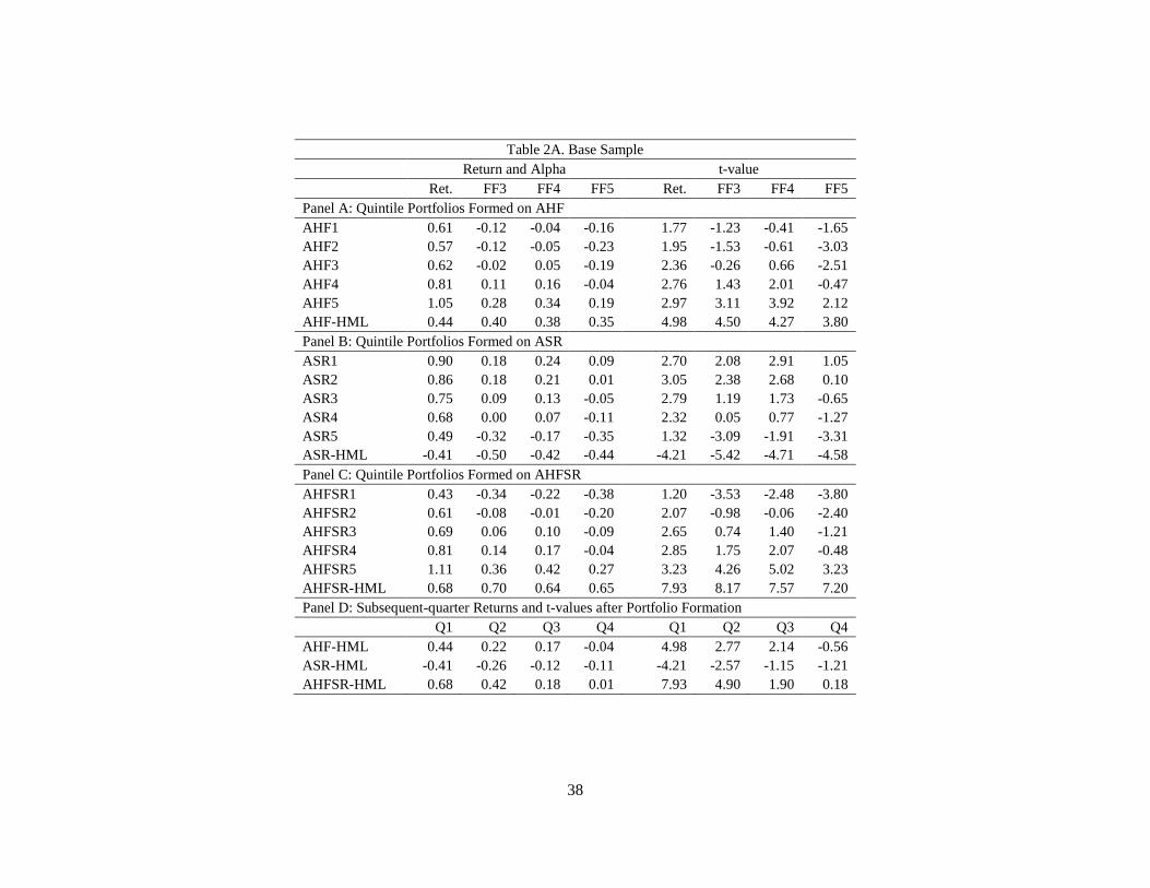
38

Table 2A. Base Sample

Return and Alpha t-value

Ret. FF3 FF4 FF5 Ret. FF3 FF4 FF5

Panel A: Quintile Portfolios Formed on AHF

AHF1 0.61 -0.12 -0.04 -0.16 1.77 -1.23 -0.41 -1.65

AHF2 0.57 -0.12 -0.05 -0.23 1.95 -1.53 -0.61 -3.03

AHF3 0.62 -0.02 0.05 -0.19 2.36 -0.26 0.66 -2.51

AHF4 0.81 0.11 0.16 -0.04 2.76 1.43 2.01 -0.47

AHF5 1.05 0.28 0.34 0.19 2.97 3.11 3.92 2.12

AHF-HML 0.44 0.40 0.38 0.35 4.98 4.50 4.27 3.80

Panel B: Quintile Portfolios Formed on ASR

ASR1 0.90 0.18 0.24 0.09 2.70 2.08 2.91 1.05

ASR2 0.86 0.18 0.21 0.01 3.05 2.38 2.68 0.10

ASR3 0.75 0.09 0.13 -0.05 2.79 1.19 1.73 -0.65

ASR4 0.68 0.00 0.07 -0.11 2.32 0.05 0.77 -1.27

ASR5 0.49 -0.32 -0.17 -0.35 1.32 -3.09 -1.91 -3.31

ASR-HML -0.41 -0.50 -0.42 -0.44 -4.21 -5.42 -4.71 -4.58

Panel C: Quintile Portfolios Formed on AHFSR

AHFSR1 0.43 -0.34 -0.22 -0.38 1.20 -3.53 -2.48 -3.80

AHFSR2 0.61 -0.08 -0.01 -0.20 2.07 -0.98 -0.06 -2.40

AHFSR3 0.69 0.06 0.10 -0.09 2.65 0.74 1.40 -1.21

AHFSR4 0.81 0.14 0.17 -0.04 2.85 1.75 2.07 -0.48

AHFSR5 1.11 0.36 0.42 0.27 3.23 4.26 5.02 3.23

AHFSR-HML 0.68 0.70 0.64 0.65 7.93 8.17 7.57 7.20

Panel D: Subsequent-quarter Returns and t-values after Portfolio Formation

Q1 Q2 Q3 Q4 Q1 Q2 Q3 Q4

AHF-HML 0.44 0.22 0.17 -0.04 4.98 2.77 2.14 -0.56

ASR-HML -0.41 -0.26 -0.12 -0.11 -4.21 -2.57 -1.15 -1.21

AHFSR-HML 0.68 0.42 0.18 0.01 7.93 4.90 1.90 0.18

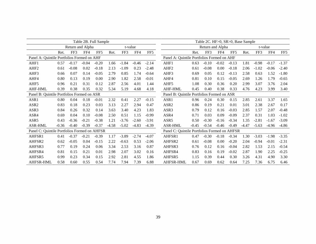
39

Table 2B. Full Sample Table 2C. HF>0, SR>0, Base Sample

Return and Alpha t-value

Return and Alpha t-value

Ret. FF3 FF4 FF5 Ret. FF3 FF4 FF5

Ret. FF3 FF4 FF5 Ret. FF3 FF4 FF5

Panel A: Quintile Portfolios Formed on AHF

Panel A: Quintile Portfolios Formed on AHF

AHF1 0.57 -0.17 -0.04 -0.20 1.66 -1.84 -0.46 -2.14

AHF1 0.63 -0.10 -0.02 -0.13 1.81 -0.98 -0.17 -1.37

AHF2 0.61 -0.08 0.02 -0.18 2.13 -1.09 0.23 -2.48

AHF2 0.61 -0.08 0.00 -0.18 2.06 -1.02 -0.06 -2.40

AHF3 0.66 0.07 0.14 -0.05 2.79 0.85 1.74 -0.64

AHF3 0.69 0.05 0.12 -0.13 2.58 0.63 1.52 -1.80

AHF4 0.80 0.13 0.19 0.00 2.90 1.82 2.58 -0.01

AHF4 0.81 0.10 0.15 -0.05 2.69 1.26 1.79 -0.65

AHF5 0.96 0.21 0.31 0.12 2.87 2.56 4.01 1.44

AHF5 1.08 0.30 0.36 0.20 2.99 3.07 3.76 2.04

AHF-HML 0.39 0.38 0.35 0.32 5.34 5.19 4.68 4.18

AHF-HML 0.45 0.40 0.38 0.33 4.76 4.23 3.99 3.40

Panel B: Quintile Portfolios Formed on ASR

Panel B: Quintile Portfolios Formed on ASR

ASR1 0.80 0.04 0.18 -0.01 2.32 0.41 2.27 -0.15

ASR1 0.96 0.24 0.30 0.15 2.85 2.61 3.37 1.65

ASR2 0.83 0.18 0.23 0.03 3.13 2.27 2.94 0.47

ASR2 0.86 0.19 0.21 0.01 3.01 2.38 2.67 0.17

ASR3 0.84 0.26 0.32 0.14 3.63 3.40 4.23 1.83

ASR3 0.79 0.12 0.16 -0.03 2.85 1.57 2.07 -0.48

ASR4 0.69 0.04 0.10 -0.08 2.50 0.51 1.15 -0.99

ASR4 0.71 0.03 0.09 -0.09 2.37 0.31 1.03 -1.02

ASR5 0.43 -0.36 -0.21 -0.38 1.21 -3.76 -2.60 -3.91

ASR5 0.50 -0.30 -0.16 -0.34 1.35 -2.81 -1.67 -3.09

ASR-HML -0.36 -0.40 -0.39 -0.37 -4.58 -5.02 -4.83 -4.39

ASR-HML -0.45 -0.54 -0.46 -0.49 -4.47 -5.63 -4.96 -4.86

Panel C: Quintile Portfolios Formed on AHFSR

Panel C: Quintile Portfolios Formed on AHFSR

AHFSR1 0.41 -0.37 -0.21 -0.39 1.17 -3.89 -2.74 -4.07

AHFSR1 0.47 -0.30 -0.18 -0.34 1.30 -3.03 -1.98 -3.35

AHFSR2 0.62 -0.05 0.04 -0.15 2.22 -0.63 0.53 -2.06

AHFSR2 0.61 -0.08 0.00 -0.20 2.04 -0.94 -0.01 -2.31

AHFSR3 0.77 0.19 0.24 0.06 3.34 2.53 3.16 0.87

AHFSR3 0.76 0.12 0.16 -0.04 2.82 1.53 2.15 -0.54

AHFSR4 0.81 0.15 0.21 0.01 2.98 2.07 3.02 0.16

AHFSR4 0.83 0.16 0.19 -0.02 2.87 1.90 2.25 -0.25

AHFSR5 0.99 0.23 0.34 0.15 2.92 2.81 4.55 1.86

AHFSR5 1.15 0.39 0.44 0.30 3.26 4.31 4.90 3.30

AHFSR-HML 0.58 0.60 0.55 0.54 7.74 7.94 7.39 6.88 AHFSR-HML 0.67 0.69 0.62 0.64 7.25 7.36 6.75 6.46

40

Table 2D. First Half of the Sample Period, 1990Q1–2000Q2 Table 2E. Second Half of the Sample Period, 2000Q3–2012Q4

Return and Alpha t-value

Return and Alpha t-value

Ret. FF3 FF4 FF5 Ret. FF3 FF4 FF5

Ret. FF3 FF4 FF5 Ret. FF3 FF4 FF5

Panel A: Quintile Portfolios Formed on AHF

Panel A: Quintile Portfolios Formed on AHF

AHF1 0.77 -0.19 -0.01 -0.18 1.67 -1.28 -0.04 -1.21

AHF1 0.47 -0.14 -0.13 -0.10 0.90 -1.26 -1.17 -0.89

AHF2 0.69 -0.23 -0.03 -0.28 1.91 -1.79 -0.29 -2.52

AHF2 0.48 -0.05 -0.05 -0.08 1.04 -0.62 -0.57 -0.88

AHF3 0.70 -0.14 0.03 -0.21 2.24 -1.06 0.28 -1.82

AHF3 0.54 0.07 0.08 -0.04 1.30 1.02 1.04 -0.56

AHF4 0.94 0.01 0.15 -0.05 2.64 0.12 1.33 -0.43

AHF4 0.69 0.15 0.15 0.08 1.48 1.96 1.89 0.98

AHF5 1.15 0.10 0.19 0.05 2.45 0.72 1.34 0.37

AHF5 0.96 0.38 0.40 0.44 1.84 4.12 4.60 4.52

AHF-HML 0.38 0.29 0.20 0.23 3.10 2.39 1.62 1.76

AHF-HML 0.50 0.52 0.53 0.54 3.99 4.22 4.29 4.27

Panel B: Quintile Portfolios Formed on ASR

Panel B: Quintile Portfolios Formed on ASR

ASR1 1.05 0.09 0.27 0.09 2.42 0.66 2.05 0.71

ASR1 0.75 0.21 0.21 0.20 1.50 2.36 2.36 2.18

ASR2 1.04 0.14 0.26 0.05 3.00 1.19 2.20 0.46

ASR2 0.69 0.17 0.16 0.06 1.57 2.09 2.00 0.74

ASR3 0.83 -0.03 0.08 -0.10 2.58 -0.26 0.70 -0.94

ASR3 0.69 0.19 0.18 0.09 1.61 2.24 2.20 1.10

ASR4 0.72 -0.21 -0.04 -0.23 1.94 -1.61 -0.34 -1.94

ASR4 0.66 0.15 0.15 0.12 1.45 1.65 1.63 1.22

ASR5 0.63 -0.41 -0.21 -0.45 1.32 -2.62 -1.41 -2.93

ASR5 0.35 -0.30 -0.26 -0.16 0.62 -2.38 -2.51 -1.25

ASR-HML -0.41 -0.50 -0.47 -0.55 -3.44 -4.44 -4.03 -4.56

ASR-HML -0.41 -0.51 -0.46 -0.37 -2.67 -3.47 -3.65 -2.40

Panel C: Quintile Portfolios Formed on AHFSR

Panel C: Quintile Portfolios Formed on AHFSR

AHFSR1 0.54 -0.47 -0.27 -0.48 1.14 -3.10 -1.91 -3.15

AHFSR1 0.34 -0.30 -0.27 -0.22 0.62 -2.66 -2.72 -1.85

AHFSR2 0.72 -0.21 -0.01 -0.24 1.98 -1.59 -0.07 -2.04

AHFSR2 0.51 -0.01 -0.01 -0.04 1.12 -0.12 -0.09 -0.51

AHFSR3 0.85 0.02 0.17 -0.06 2.73 0.19 1.54 -0.58

AHFSR3 0.56 0.08 0.08 -0.01 1.35 0.97 0.92 -0.10

AHFSR4 0.94 0.02 0.14 -0.05 2.65 0.20 1.12 -0.49

AHFSR4 0.69 0.19 0.18 0.09 1.56 2.56 2.48 1.17

AHFSR5 1.21 0.20 0.31 0.17 2.65 1.46 2.29 1.35

AHFSR5 1.03 0.45 0.46 0.49 2.00 5.09 5.29 5.13

AHFSR-HML 0.67 0.67 0.57 0.65 5.93 5.77 4.99 5.27 AHFSR-HML 0.69 0.75 0.73 0.70 5.38 5.85 5.93 5.18

41

Table 2F. Double Sorting on AHF and ASR

Return and Alpha t-value

AHF1 AHF2 AHF3 AHF-HML AHF1 AHF2 AHF3 AHF-HML

Panel A: Excess Returns

ASR1 0.71 0.72 1.18 0.47 2.12 2.55 3.47 4.41

ASR2 0.67 0.67 0.98 0.30 2.29 2.74 3.26 3.73

ASR3 0.40 0.45 0.81 0.42 1.13 1.48 2.25 4.75

ASR-HML -0.31 -0.27 -0.36 -3.43 -2.80 -3.73

Panel B: FF3 Alpha

ASR1 0.01 0.05 0.42 0.41 0.11 0.56 4.36 3.91

ASR2 -0.02 0.07 0.28 0.30 -0.22 0.86 2.88 3.60

ASR3 -0.37 -0.26 0.03 0.40 -3.51 -2.72 0.31 4.56

ASR-HML -0.38 -0.31 -0.39 -4.35 -3.31 -4.09

Panel C: FF4 Alpha

ASR1 0.08 0.08 0.47 0.39 0.88 0.87 4.94 3.66

ASR2 0.02 0.12 0.30 0.28 0.27 1.52 3.10 3.33

ASR3 -0.25 -0.14 0.12 0.38 -2.57 -1.60 1.32 4.25

ASR-HML -0.34 -0.22 -0.35 -3.86 -2.43 -3.65

Panel D: FF5 Alpha

ASR1 -0.04 -0.13 0.29 0.33 -0.42 -1.52 2.93 3.04

ASR2 -0.11 -0.11 0.12 0.23 -1.24 -1.46 1.27 2.64

ASR3 -0.41 -0.38 -0.02 0.39 -3.97 -3.84 -0.22 4.25

ASR-HML -0.37 -0.25 -0.31 -3.99 -2.49 -3.12

42

Table 2G. One Dimensional Sorting from AHFSRIO

Return and Alpha t-value

Ret. FF3 FF4 FF5 Ret. FF3 FF4 FF5

Panel A: Quintile Portfolios Formed on AHFSRIO

AHFSRIO1 0.42 -0.34 -0.23 -0.35 1.19 -3.82 -2.81 -3.87

AHFSRIO2 0.62 -0.08 0.00 -0.21 2.09 -0.94 -0.02 -2.49

AHFSRIO3 0.71 0.05 0.11 -0.11 2.60 0.68 1.48 -1.49

AHFSRIO4 0.86 0.18 0.22 0.02 2.98 2.25 2.65 0.27

AHFSRIO5 1.06 0.32 0.37 0.23 3.16 3.94 4.60 2.83

AHFSRIO-HML 0.64 0.66 0.60 0.58 7.46 7.74 7.14 6.54

Panel B: Subsequent-quarter Returns and t-values after Portfolio Formation

Ret t-value

Quarters Q1 Q2 Q3 Q4 Q1 Q2 Q3 Q4

AHFSRIO-HML 0.64 0.42 0.22 0.03 7.46 4.85 2.35 0.32

43

Table 2H. Double Sorting from AIO and ASR

Ret. and Alpha t-value

AIO1 AIO2 AIO3 AIO-HML AIO1 AIO2 AIO3 AIO-HML

Panel A: Excess Returns

ASR1 0.89 0.82 0.80 -0.09 2.72 2.88 2.36 -0.74

ASR2 0.84 0.71 0.76 -0.08 3.03 2.75 2.50 -0.80

ASR3 0.59 0.58 0.60 0.00 1.62 1.84 1.65 0.03

ASR-HML -0.30 -0.24 -0.21 -2.83 -2.42 -2.04

Panel B: FF3 Alpha

ASR1 0.17 0.16 0.08 -0.09 1.74 1.75 0.80 -0.76

ASR2 0.18 0.07 0.06 -0.12 1.99 0.89 0.68 -1.25

ASR3 -0.19 -0.16 -0.17 0.02 -1.41 -1.41 -1.90 0.17

ASR-HML -0.36 -0.32 -0.25 -3.50 -3.20 -2.54

Panel C: FF4 Alpha

ASR1 0.28 0.18 0.04 -0.25 3.16 1.93 0.37 -2.40

ASR2 0.28 0.11 0.05 -0.23 3.31 1.39 0.57 -2.61

ASR3 0.05 -0.01 -0.15 -0.20 0.49 -0.09 -1.64 -1.85

ASR-HML -0.23 -0.19 -0.19 -2.47 -2.12 -1.92

Panel D: FF5 Alpha

ASR1 0.05 -0.01 0.02 -0.03 0.51 -0.16 0.21 -0.23

ASR2 0.07 -0.12 -0.06 -0.13 0.78 -1.64 -0.60 -1.28

ASR3 -0.23 -0.29 -0.20 0.02 -1.61 -2.58 -2.22 0.17

ASR-HML -0.28 -0.27 -0.23 -2.55 -2.63 -2.15

Panel E: Subsequent quarter returns and t-values

Ret t-value

Quarters Q1 Q2 Q3 Q4 Q1 Q2 Q3 Q4

AIO3, ASR1 0.80 0.81 0.74 1.02 2.36 2.29 2.03 2.74

AIO1, ASR3 0.59 0.87 0.81 1.08 1.62 2.31 2.15 2.82

Diff. 0.21 -0.06 -0.07 -0.06 1.35 -0.37 -0.46 -0.42

Alpha t-value

AIO3, ASR1 0.02 0.01 -0.04 0.09 0.21 0.11 -0.33 0.62

AIO1, ASR3 -0.23 0.05 -0.09 0.00 -1.61 0.35 -0.67 -0.02

Diff. 0.25 -0.04 0.05 0.09 1.51 -0.25 0.38 0.63

44

Table 3. Fama-MacBeth Regressions of Monthly Excess Returns

This table presents the Fama-MacBeth regression results from regressing average monthly stock excess returns over the next quarter on AHF, ASR,

or AHFSR of the current quarter. The control variables include book-to-market ratio (BM) of Fama and French (2008); gross profitability (GP) of

Novy-Marx (2013); operating profit (OP) of Fama and French (2015); momentum (MOM) of Jegadeesh and Titman (1993); market capitalization

(MC) of Fama and French (2008); asset growth (AG) of Cooper, Gulen, and Schill (2008), Hou, Xue, and Zhang (2014), and Fama and French

(2015); investment growth (IK) of Xing (2008); net stock issues (NS) of Fama and French (2008); accrual (AC) of Fama and French (2008); and

net operating assets (NOA) of Hirshleifer, Hou, Teoh, and Zhang (2004). We take natural logs for BM and MC. All explanatory variables are

winsorized at 1% and 99% and standardized at the end of each quarter. Stock excess returns are in percent in month. The t-values use Newey-West

standard errors with four lags. The sample period is from 1990Q1 to 2012Q4.

45

Table 3, continued.

Fama-MacBeth Regression of Future Stock Excess Returns on AHF, ASR, or AHFSR

Panel A: 1990Q1–2012Q4 Panel B: 1990Q1–2012Q4, HF>0,

SR>0 Panel C: 1990Q1–2000Q2 Panel D: 2000Q3–2012Q4

AHF 0.15***

0.16***

0.12***

0.17***

t-value 5.39

5.46

2.81

6.31

ASR -0.14***

-0.16***

-0.18***

-0.12***

t-value -4.10

-4.23

-2.81

-3.38

AHFSR

0.22***

0.24***

0.23***

0.22***

t-value

5.82

6.17

3.24

6.87

BM 0.12 0.11 0.11 0.12 0.11 0.11 0.01 -0.01 -0.01 0.12 0.21 0.21

t-value 1.35 1.22 1.21 1.26 1.12 1.12 0.09 -0.02 -0.04 1.59 1.54 1.55

OP 0.08 0.08 0.08 0.09 0.07 0.08 -0.05 -0.06 -0.06 0.20* 0.20* 0.21*

t-value 0.95 0.87 0.91 0.94 0.83 0.88 -0.33 -0.41 -0.4 1.75 1.71 1.74

MOM 0.01 0.01 0.01 -0.02 -0.01 -0.01 0.32*** 0.34*** 0.33*** -0.26 -0.27 -0.26

t-value 0.01 0.04 0.03 -0.14 -0.09 -0.11 3.16 3.29 3.25 -1.48 -1.55 -1.51

MC -0.08 -0.09 -0.09 -0.10 -0.12* -0.11* -0.02 -0.04 -0.03 -0.13** -0.15*** -0.15***

t-value -1.24 -1.57 -1.45 -1.55 -1.93 -1.74 -0.21 -0.34 -0.25 -2.36 -2.90 -2.81

AG 0.02 0.03 0.03 0.04 0.04 0.04 0.08 0.09 0.09 -0.05 -0.05 -0.05

t-value 0.35 0.45 0.44 0.54 0.61 0.62 0.77 0.82 0.81 -0.63 -0.56 -0.56

IK -0.01 -0.01 -0.01 -0.02 -0.02 -0.02 0.01 0.01 0.01 -0.04 -0.04 -0.04

t-value -0.47 -0.36 -0.42 -0.57 -0.47 -0.53 0.2 0.31 0.31 -1.05 -0.99 -1.07

GP 0.03 0.03 0.03 0.03 0.03* 0.03 0.04 0.04 0.04 0.02 0.02 0.02

t-value 1.49 1.48 1.44 1.66 1.67 1.62 1.61 1.54 1.53 0.54 0.57 0.53

NS -0.05 -0.06 -0.05 -0.05 -0.06 -0.06 -0.05 -0.05 -0.05 -0.05 -0.05 -0.05

t-value -1.26 -1.4 -1.35 -1.15 -1.23 -1.21 -0.86 -0.95 -0.98 -0.88 -0.97 -0.89

AC 0.02 0.03 0.03 0.03 0.03 0.03 -0.01 -0.00 0.01 0.03 0.04 0.04

t-value 1.02 1.17 1.14 1.34 1.55 1.48 -0.09 0.03 0.06 1.14 1.24 1.19

NOA -0.20** -0.20** -0.20** -0.20** -0.20** -0.20** -0.34** -0.34** -0.34** -0.05 -0.06 -0.06

t-value -2.43 -2.46 -2.44 -2.49 -2.53 -2.50 -2.46 -2.48 -2.44 -0.83 -0.86 -0.87

Const. 0.79*** 0.79*** 0.79*** 0.82*** 0.82*** 0.82*** 0.84*** 0.84*** 0.84*** 0.72 0.72 0.72

t-value 2.85 2.85 2.84 2.94 2.93 2.93 3.01 3.00 3.00 1.62 1.61 1.61

Adj. R2 0.083 0.083 0.084 0.088 0.089 0.089 0.073 0.074 0.074 0.090 0.090 0.091

Obs. 115,461 115,461 115,461 101,993 101,993 101,993 55,355 55,355 55,355 61,512 61,512 61,512

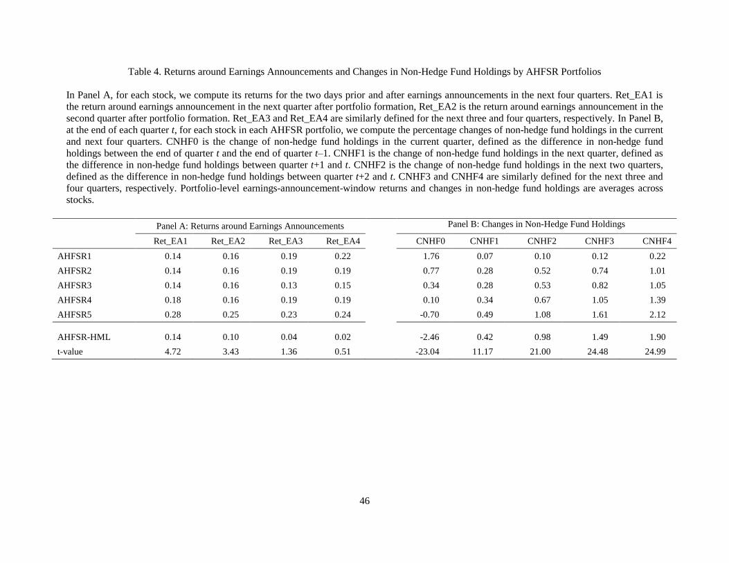
46

Table 4. Returns around Earnings Announcements and Changes in Non-Hedge Fund Holdings by AHFSR Portfolios

In Panel A, for each stock, we compute its returns for the two days prior and after earnings announcements in the next four quarters. Ret_EA1 is

the return around earnings announcement in the next quarter after portfolio formation, Ret_EA2 is the return around earnings announcement in the

second quarter after portfolio formation. Ret_EA3 and Ret_EA4 are similarly defined for the next three and four quarters, respectively. In Panel B,

at the end of each quarter t, for each stock in each AHFSR portfolio, we compute the percentage changes of non-hedge fund holdings in the current

and next four quarters. CNHF0 is the change of non-hedge fund holdings in the current quarter, defined as the difference in non-hedge fund

holdings between the end of quarter t and the end of quarter t–1. CNHF1 is the change of non-hedge fund holdings in the next quarter, defined as

the difference in non-hedge fund holdings between quarter t+1 and t. CNHF2 is the change of non-hedge fund holdings in the next two quarters,

defined as the difference in non-hedge fund holdings between quarter t+2 and t. CNHF3 and CNHF4 are similarly defined for the next three and

four quarters, respectively. Portfolio-level earnings-announcement-window returns and changes in non-hedge fund holdings are averages across

stocks.

Panel A: Returns around Earnings Announcements Panel B: Changes in Non-Hedge Fund Holdings

Ret_EA1 Ret_EA2 Ret_EA3 Ret_EA4 CNHF0 CNHF1 CNHF2 CNHF3 CNHF4

AHFSR1 0.14 0.16 0.19 0.22 1.76 0.07 0.10 0.12 0.22

AHFSR2 0.14 0.16 0.19 0.19 0.77 0.28 0.52 0.74 1.01

AHFSR3 0.14 0.16 0.13 0.15 0.34 0.28 0.53 0.82 1.05

AHFSR4 0.18 0.16 0.19 0.19 0.10 0.34 0.67 1.05 1.39

AHFSR5 0.28 0.25 0.23 0.24 -0.70 0.49 1.08 1.61 2.12

AHFSR-HML 0.14 0.10 0.04 0.02 -2.46 0.42 0.98 1.49 1.90

t-value 4.72 3.43 1.36 0.51 -23.04 11.17 21.00 24.48 24.99

47

Table 5. Net Arbitrage Trading and Stock Anomaly Returns in the Following Year

For each return anomaly, at the end of each quarter, we construct quintile portfolios and compute monthly portfolio returns in the next four

quarters (Q1, Q2, Q3 and Q4). In Panel A, LMS is the return spread between the long- and the short-legs of the stock anomalies. The column

“Avg.” reports results for a portfolio equally-investing in the 10 anomalies. We also report the alpha of the long-minus-short of these composite

portfolios, Alpha(LMS), as well as the alphas of the long portfolio Alpha(L) and the short portfolio Alpha(S), based on the Fama-French (2015)

five-factor model. Next, we independently form three AHFSR portfolios using the 30% and 70% AHFSR cutoff values. At the end of each quarter,

in the long leg, we identify stocks that belong to the AHFSR group 3 (Trading) and that do not belong to AHFSR group 3 (Not Trading). Similarly,

in the short leg, we identify those stocks that belong to the AHFSR group 1 (Trading) and that do not belong to the AHFSR group 1 (Not Trading).

We track the monthly equal-weighted averages of these four portfolios. In Panel B, “return of trading” is the return spread between the long- and

the short-legs when arbitrage capital trades. In Panel C, “return of not trading” is the return spread between the long- and short-legs when arbitrage

capital does not trade. Panel D reports the difference between the groups of trading and not-trading. Table 5A presents the returns, and Table 5B

presents corresponding t-values. Table 5C presents, for each return anomaly, the total number of stocks on the long- or the short-leg, and the

numbers and fractions of stocks that are traded by the arbitrage capital on the long- or the short-leg. We consider the following anomalies: book-

to-market ratio (BM) of Fama and French (2008); gross profitability (GP) of Novy-Marx (2013); operating profit (OP) of Fama and French (2015);

momentum (MOM) of Jegadeesh and Titman (1993); market capitalization (MC) of Fama and French (2008); asset growth (AG) of Cooper, Gulen,

and Schill (2008), Hou, Xue, and Zhang (2014), and Fama and French (2015); investment growth (IK) of Xing (2008); net stock issues (NS) of

Fama and French (2008); accrual (AC) of Fama and French (2008); and net operating assets (NOA) of Hirshleifer, Hou, Teoh, and Zhang (2004).

The sample period is from 1990Q1 to 2012Q4.

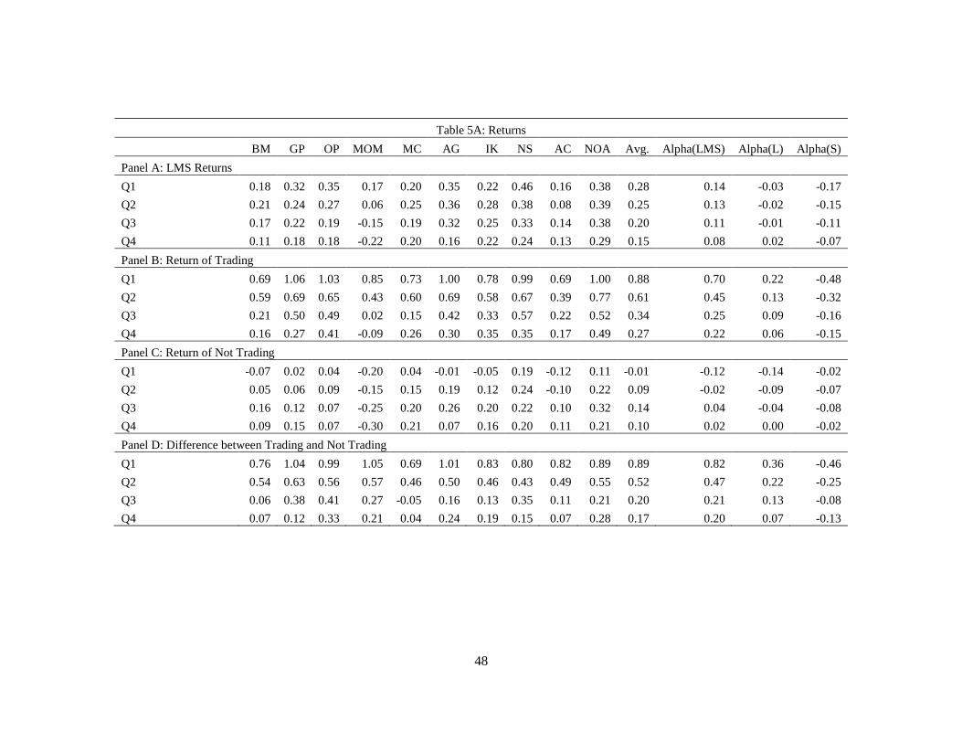
48

Table 5A: Returns

BM GP OP MOM MC AG IK NS AC NOA Avg. Alpha(LMS) Alpha(L) Alpha(S)

Panel A: LMS Returns

Q1 0.18 0.32 0.35 0.17 0.20 0.35 0.22 0.46 0.16 0.38 0.28 0.14 -0.03 -0.17

Q2 0.21 0.24 0.27 0.06 0.25 0.36 0.28 0.38 0.08 0.39 0.25 0.13 -0.02 -0.15

Q3 0.17 0.22 0.19 -0.15 0.19 0.32 0.25 0.33 0.14 0.38 0.20 0.11 -0.01 -0.11

Q4 0.11 0.18 0.18 -0.22 0.20 0.16 0.22 0.24 0.13 0.29 0.15 0.08 0.02 -0.07

Panel B: Return of Trading

Q1 0.69 1.06 1.03 0.85 0.73 1.00 0.78 0.99 0.69 1.00 0.88 0.70 0.22 -0.48

Q2 0.59 0.69 0.65 0.43 0.60 0.69 0.58 0.67 0.39 0.77 0.61 0.45 0.13 -0.32

Q3 0.21 0.50 0.49 0.02 0.15 0.42 0.33 0.57 0.22 0.52 0.34 0.25 0.09 -0.16

Q4 0.16 0.27 0.41 -0.09 0.26 0.30 0.35 0.35 0.17 0.49 0.27 0.22 0.06 -0.15

Panel C: Return of Not Trading

Q1 -0.07 0.02 0.04 -0.20 0.04 -0.01 -0.05 0.19 -0.12 0.11 -0.01 -0.12 -0.14 -0.02

Q2 0.05 0.06 0.09 -0.15 0.15 0.19 0.12 0.24 -0.10 0.22 0.09 -0.02 -0.09 -0.07

Q3 0.16 0.12 0.07 -0.25 0.20 0.26 0.20 0.22 0.10 0.32 0.14 0.04 -0.04 -0.08

Q4 0.09 0.15 0.07 -0.30 0.21 0.07 0.16 0.20 0.11 0.21 0.10 0.02 0.00 -0.02

Panel D: Difference between Trading and Not Trading

Q1 0.76 1.04 0.99 1.05 0.69 1.01 0.83 0.80 0.82 0.89 0.89 0.82 0.36 -0.46

Q2 0.54 0.63 0.56 0.57 0.46 0.50 0.46 0.43 0.49 0.55 0.52 0.47 0.22 -0.25

Q3 0.06 0.38 0.41 0.27 -0.05 0.16 0.13 0.35 0.11 0.21 0.20 0.21 0.13 -0.08

Q4 0.07 0.12 0.33 0.21 0.04 0.24 0.19 0.15 0.07 0.28 0.17 0.20 0.07 -0.13

49

Table 5B: t-values

BM GP OP MOM MC AG IK NS AC NOA Avg. Alpha(LMS) Alpha(L) Alpha(S)

Panel A: LMS Returns

Q1 0.82 1.86 2.03 0.54 0.97 2.25 1.92 2.70 1.71 2.50 3.47 2.27 -0.49 -1.92

Q2 0.99 1.37 1.44 0.20 1.30 2.31 2.32 2.19 0.86 2.53 3.19 1.99 -0.36 -1.58

Q3 0.78 1.21 1.11 -0.62 0.99 1.90 1.82 1.85 1.51 2.45 2.48 1.46 -0.07 -1.04

Q4 0.55 0.99 1.02 -0.96 0.99 0.97 1.64 1.36 1.41 1.86 1.97 1.18 0.19 -0.62

Panel B: Return of Trading

Q1 2.68 5.12 4.11 2.51 3.09 5.22 4.63 4.47 5.10 5.13 7.10 6.31 2.99 -4.37

Q2 2.29 3.24 2.70 1.33 2.59 3.54 3.43 2.99 2.71 4.29 4.88 3.90 1.54 -2.63

Q3 0.83 2.24 2.19 0.08 0.65 2.00 1.86 2.52 1.47 2.78 2.68 1.98 0.99 -1.20

Q4 0.64 1.15 1.76 -0.34 1.04 1.49 1.96 1.51 1.17 2.78 2.18 1.73 0.60 -1.16

Panel C: Return of Not Trading

Q1 -0.35 0.11 0.25 -0.64 0.21 -0.07 -0.44 1.23 -1.21 0.72 -0.07 -1.75 -2.36 -0.21

Q2 0.25 0.33 0.54 -0.52 0.76 1.22 0.98 1.50 -1.04 1.39 1.16 -0.30 -1.36 -0.75

Q3 0.74 0.65 0.44 -1.02 1.06 1.54 1.46 1.26 1.04 1.94 1.72 0.55 -0.57 -0.81

Q4 0.44 0.84 0.44 -1.34 1.12 0.39 1.13 1.18 1.09 1.21 1.27 0.28 -0.03 -0.22

Panel D: Difference between Trading and Not Trading

Q1 5.19 6.48 5.76 7.25 4.41 6.98 5.11 5.19 5.81 5.57 7.85 6.92 5.52 -5.93

Q2 3.84 3.93 3.53 3.74 3.12 3.62 2.85 3.03 3.36 3.61 4.69 3.99 3.33 -3.27

Q3 0.38 2.23 2.73 1.66 -0.33 1.02 0.82 2.28 0.74 1.26 1.72 1.67 1.96 -1.00

Q4 0.47 0.65 2.13 1.33 0.29 1.45 1.14 0.90 0.44 1.66 1.44 1.54 0.98 -1.55

50

Table 5C: Number and Fraction of Stocks Traded by Arbitrage Capital

BM GP OP MOM MC AG IK NS AC NOA

# of Stocks Traded by Arbitrage Capital, Long Leg 92 102 95 106 99 104 92 91 87 89

Fraction of Stocks Traded by Arbitrage Capital, Long Leg 0.29 0.32 0.30 0.33 0.31 0.33 0.33 0.29 0.34 0.28

# of Stocks Traded by Arbitrage Capital, Short Leg 95 83 108 102 71 116 101 113 90 109

Fraction of Stocks Traded by Arbitrage Capital, Short Leg 0.30 0.26 0.33 0.31 0.22 0.37 0.36 0.36 0.35 0.34

# of Stocks on the Long or he Short Leg 322 322 322 322 322 315 281 315 254 314

51

Table 6. Differences in Characteristics of Anomaly Stocks Traded and Not Traded by Arbitrage Capital

At the end of each quarter, on the long leg of each anomaly, we identify a portfolio of stocks that have high AHFSR (ranked among the top 30%)

as stocks treated by arbitrageurs. Similarly, we identify a portfolio of stocks that have low AHFSR (ranked among the bottom 30%) as stocks not

traded by arbitrageurs. For these two portfolios, we compute portfolio-level price, idiosyncratic volatility, the Amihud (2002) illiquidity measure,

and anomaly characteristic, by equal-averaging stocks in each portfolio. The Amihud measure is transformed into percentiles among

NYSE/AMEX or NASDAQ firms separately. Panel A presents the difference in these characteristics between the “Trading” portfolio and “Not

Trading” portfolio for the long-leg of each anomaly. The difference of “Anomaly Char.” in each anomaly is normalized by the average of cross-

sectional standard deviation of the anomaly variable. Panel B repeats this analysis for the short-leg. Panels C and D report corresponding t-values.

BM GP OP MOM MC AG IK NS AC NOA Average

Panel A: Trading–Not Trading, Long Leg

Price -3.48 -1.94 -1.22 -0.61 -1.62 -1.80 -1.98 -2.26 -1.70 0.11 -1.65

IVOL 0.01 0.01 0.01 0.00 0.02 0.01 0.01 0.01 0.01 0.02 0.01

Amihud 15.94 25.65 26.55 26.88 10.90 19.78 20.64 21.48 22.78 26.94 21.75

Anomaly Char. -0.05 -0.03 -0.03 -0.05 0.00 0.02 0.01 0.04 0.10 0.00

Panel B: Trading–Not Trading, Short Leg

Price -4.64 -3.91 -2.84 -0.21 -3.15 -3.04 -1.92 -2.13 -1.10 -1.58 -2.45

IVOL 0.02 0.02 0.02 0.01 0.01 0.01 0.01 0.02 0.01 0.01 0.01

Amihud 34.34 23.74 21.62 20.56 39.38 27.96 23.51 25.99 20.86 22.75 26.07

Anomaly Char. 0.01 0.05 0.13 0.09 0.03 -0.17 -0.13 -0.11 -0.06 -0.12

Panel C: Trading–Not Trading, Long Leg, t-values

Price -9.81 -5.48 -2.32 -1.27 -5.37 -4.90 -3.88 -4.84 -3.52 0.17 -6.51

IVOL 15.52 17.46 15.96 5.77 16.56 15.22 16.06 16.00 11.22 15.21 20.75

Amihud 24.79 49.55 44.19 53.27 18.13 25.97 30.08 26.48 33.81 40.69 55.96

Anomaly Char. -4.12 -2.92 -1.67 -5.16 2.72 6.15 4.15 10.39 5.69 0.15

Panel D: Trading–Not Trading, Short Leg, t-values

Price -8.92 -6.72 -7.04 -0.63 -4.52 -5.48 -5.10 -5.62 -3.22 -5.53 -8.70

IVOL 19.79 11.96 18.35 8.52 12.72 14.09 16.52 19.12 13.67 18.51 20.96

Amihud 67.91 40.33 36.17 30.47 49.78 51.29 39.09 44.74 32.14 42.19 79.39

Anomaly Char. 3.86 8.24 9.97 9.85 24.17 -8.43 -5.29 -4.98 -3.96 -9.07

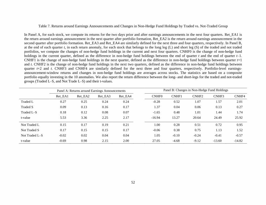
52

Table 7. Returns around Earnings Announcements and Changes in Non-Hedge Fund Holdings by Traded vs. Not-Traded Group

In Panel A, for each stock, we compute its returns for the two days prior and after earnings announcements in the next four quarters. Ret_EA1 is

the return around earnings announcement in the next quarter after portfolio formation, Ret_EA2 is the return around earnings announcement in the

second quarter after portfolio formation. Ret_EA3 and Ret_EA4 are similarly defined for the next three and four quarters, respectively. In Panel B,

at the end of each quarter t, in each return anomaly, for each stock that belongs to the long leg (L) and short leg (S) of the traded and not traded

portfolios, we compute the changes of non-hedge fund holdings in the current and next four quarters. CNHF0 is the change of non-hedge fund

holdings in the current quarter, defined as the difference in non-hedge fund holdings between the end of quarter t and the end of quarter t–1.

CNHF1 is the change of non-hedge fund holdings in the next quarter, defined as the difference in non-hedge fund holdings between quarter t+1

and t. CNHF2 is the change of non-hedge fund holdings in the next two quarters, defined as the difference in non-hedge fund holdings between

quarter t+2 and t. CNHF3 and CNHF4 are similarly defined for the next three and four quarters, respectively. Portfolio-level earnings-

announcement-window returns and changes in non-hedge fund holdings are averages across stocks. The statistics are based on a composite

portfolio equally investing in the 10 anomalies. We also report the return difference between the long- and short-legs for the traded and not-traded

groups (Traded L–S, and Not Trade L–S) and their t-values.

Panel A: Returns around Earnings Announcements Panel B: Changes in Non-Hedge Fund Holdings

Ret_EA1 Ret_EA2 Ret_EA3 Ret_EA4 CNHF0 CNHF1 CNHF2 CNHF3 CNHF4

Traded L 0.27 0.25 0.24 0.24 -0.28 0.52 1.07 1.57 2.01

Traded S 0.09 0.13 0.16 0.17 1.37 0.04 0.06 0.13 0.27

Traded L–S 0.18 0.12 0.08 0.07 -1.65 0.48 1.01 1.44 1.74

t-value 5.53 3.36 2.25 2.17 -16.94 13.27 20.64 24.49 25.92

Not Traded L 0.15 0.17 0.19 0.21 1.00 0.28 0.51 0.72 0.95

Not Traded S 0.17 0.15 0.15 0.17 -0.06 0.38 0.75 1.13 1.52

Not Traded L–S -0.02 0.02 0.04 0.04 1.05 -0.10 -0.24 -0.41 -0.57

t-value -0.69 0.98 2.15 2.00 27.05 -4.68 -9.12 -13.60 -14.82

53

Figure 1. Number of Stocks and Sample Coverage

At the end of each quarter, we count the number of firms that have positive values of hedge fund holdings

(HF), positive values of short interest (SR), positive values of both HF and SR, and the total number of

stocks in our base sample, and plot them over quarters in figure (a). We compute the market capitalization

of these firms as a fraction of market capitalization of the CRSP universe, and plot them in figure (b). Our

sample does not include firms with market capitalization below the 20th percentile size breakpoint of

NYSE firms. The sample period is from 1990Q1 to 2012Q4.

800

1000

1200

1400

1600

1800

2000

2200

1990

1991

1992

1993

1994

1995

1996

1997

1998

1999

2000

2001

2002

2003

2004

2005

2006

2007

2008

2009

2010

2011

2012

Valu

e

(a) Number of Stocks

HF>0

SR>0

HF>0 and SR>0

Base Sample

0.8

0.82

0.84

0.86

0.88

0.9

0.92

0.94

0.96

0.98

1

1990

1991

1992

1993

1994

1995

1996

1997

1998

1999

2000

2001

2002

2003

2004

2005

2006

2007

2008

2009

2010

2011

2012

Valu

e

(b) MktCap Coverage of HF>0, SR>0, HF >0 and SR>0 in Our Sample

HF>0

SR>0

HF>0 and SR>0

54

Figure 2. Aggregate Variables about Hedge Fund Holdings and Short Interest

We plot value-weighted averages of the following variables: hedge fund holdings (HF), defined as the

ratio between shares owned by hedge funds and the number of outstanding shares; short interest (SR),

defined as the ratio between shares shorted and the number of shares outstanding; the difference between

HF and SR (HFSR); abnormal hedge fund holdings (AHF), defined as the percentage change of current

HF from the average of HF in the previous four quarters; abnormal short ratio (ASR), defined as the

percentage change of current SR from the average of SR in the previous four quarters; and the difference

between AHF and ASR (AHFSR). The sample period is from 1990Q1 to 2012Q4.

0

0.01

0.02

0.03

0.04

0.05

0.06

0.07

1990

1991

1992

1993

1994

1995

1996

1997

1998

1999

2000

2001

2002

2003

2004

2005

2006

2007

2008

2009

2010

2011

2012

Valu

e

(a) Aggregate HF and SR

Aggregate HF

Aggregate SR

55

Figure 2, continued.

-0.01

-0.008

-0.006

-0.004

-0.002

0

0.002

0.004

0.006

0.008

0.01

1990

1991

1992

1993

1994

1995

1996

1997

1998

1999

2000

2001

2002

2003

2004

2005

2006

2007

2008

2009

2010

2011

2012

Valu

e

(b) Aggregate AHF and ASR

Aggregate AHF

Aggregate ASR

-0.015

-0.01

-0.005

0

0.005

0.01

0.015

0.02

0.025

0.03

1990

1991

1992

1993

1994

1995

1996

1997

1998

1999

2000

2001

2002

2003

2004

2005

2006

2007

2008

2009

2010

2011

2012

Valu

e

(c) Aggregate HFSR and AHFSR

Aggregate HFSR

Aggregate AHFSR

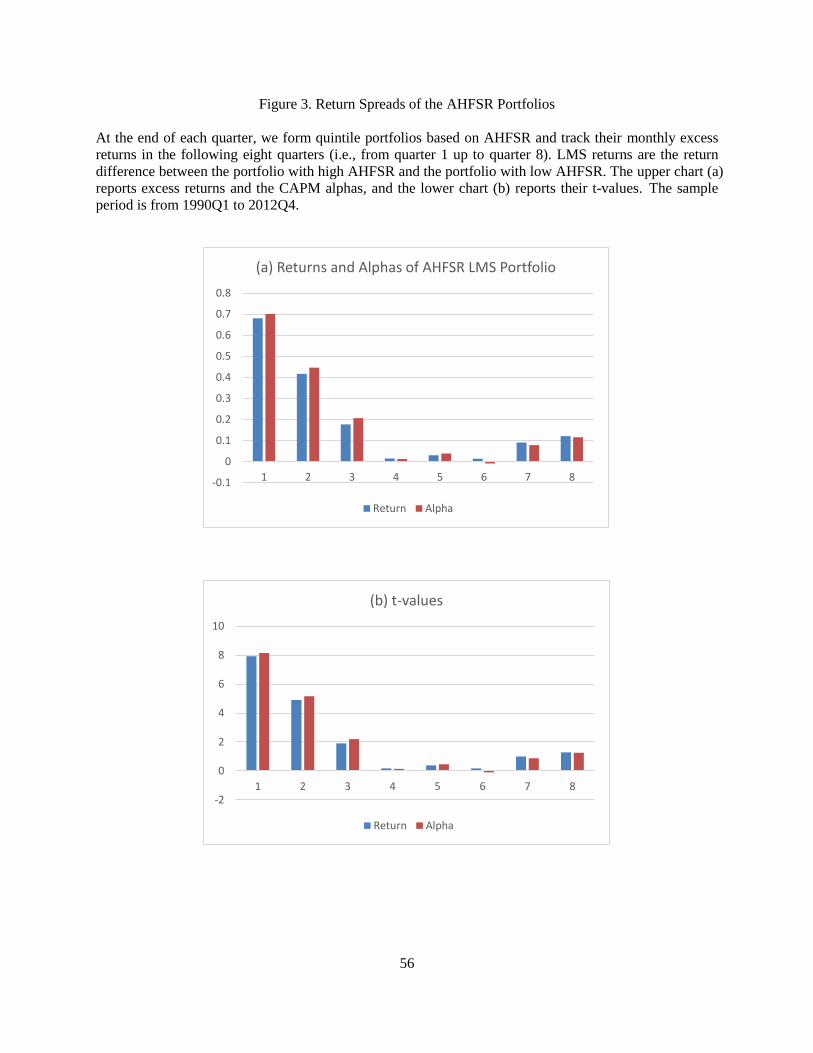
56

Figure 3. Return Spreads of the AHFSR Portfolios

At the end of each quarter, we form quintile portfolios based on AHFSR and track their monthly excess

returns in the following eight quarters (i.e., from quarter 1 up to quarter 8). LMS returns are the return

difference between the portfolio with high AHFSR and the portfolio with low AHFSR. The upper chart (a)

reports excess returns and the CAPM alphas, and the lower chart (b) reports their t-values. The sample

period is from 1990Q1 to 2012Q4.

-0.1

0

0.1

0.2

0.3

0.4

0.5

0.6

0.7

0.8

1 2 3 4 5 6 7 8

(a) Returns and Alphas of AHFSR LMS Portfolio

Return Alpha

-2

0

2

4

6

8

10

1 2 3 4 5 6 7 8

(b) t-values

Return Alpha