Arbitrage, liquidity and exit: The repo and federal funds markets

before, during, and after the financial crisis

Morten Bech, Elizabeth Klee, and Viktors Stebunovs∗

FRBNY and FRB

December 26, 2010

Abstract

This paper examines the interplay between the federal funds and repo markets, two keymarkets for monetary policy implementation, before, during, and after the financial crisis thatbegan in August 2007. Overall, the results suggest that the federal funds rate communicatedpolicy to the repo market quite well in the pre-crisis period, as well as during the first stages ofthe crisis. However, coincident with the introduction of a target range for the federal funds rateof 0 to 1/4 percent and interest on excess reserve balances, the relationship between these ratesdeteriorated, possibly due to counterparty credit concerns. Moreover, as the level of reservebalances increased dramatically, the effect of changes in these balances on market rates becamemuted. Consequently, our policy simulations suggest that a large-scale draining of reservebalances might exert weak upward pressure on the federal funds and repo rates at high levels ofbalances, but should exert strong upward pressure at lower levels.

1 Introduction

How does monetary policy implementation work? The first step is for the Federal Open Market

Committee (FOMC) to set a price for reserves. This price is called the target federal funds rate,

or the desired level for the interest rate at which depository institutions (“banks”) lend balances at

the Federal Reserve to other banks overnight.1 For many years, open market operations–purchases

and sales of U.S. Treasury and federal agency securities using repurchase agreements (repos) –were

the Federal Reserve’s most often used tool for changing the level of reserves and thus implementing

monetary policy.

After the Federal Reserve initiates the monetary policy transmission process, the most imme-

diate next step is for the federal funds rate to influence the behavior of other short-term interest

rates. In order for monetary policy transmission to be effective, these other short-term interest

rates should move with the federal funds rate. As the participants in the federal funds market and

other short-term markets frequently overlap, in theory, all rate differences should be arbitraged

∗The views expressed are those of the authors and do not reflect those of the Board of Governors, the FederalReserve Bank of New York, or the Federal Reserve System. Thanks to Jim Clouse for inspiring this research. AriMorse, Daniel Quinn, Brett Schulte, and Lisa Xu provided expert research assistance.

1Throughout this paper, we use “banks” in many places where we intend the slightly broader depository institutiondefinition.

1

away. As a result, it seems plausible that all short-term interest rates should move in tandem

with the federal funds rate. In particular, one might think that the interest rate on repurchase

agreements – the repo rate – and the federal funds rate have a special relationship, as both markets

are involved in the earliest stages of the monetary policy transmission process. Indeed, it seems

likely that these two rates would move together.

But do they? Although there are long periods when the repo rate and the federal funds rate

move together, there are also notable times when they do not. For example, figure 1 displays

the federal funds rate and the Treasury general collateral (GC) repo rate, or the rate charged on

secured overnight lending against Treasury-issued collateral. Although for much of the sample,

there appear to be only small differences between these two rates, there are spells when the spreads

widen considerably and the rate movements seem decoupled. One might question whether the

monetary policy transmission mechanism works during these periods, or whether the relationship

between the rates fundamentally changes.

In order to provide perspective on these issues, this paper characterizes the relationship between

the Treasury GC repo rate and the federal funds rate during three periods: a period of relative calm

in financial markets, from 2002 to 2007, the early stages of the financial crisis, from August 2007 to

December 2008, and post-December 2008, after the Federal Open Market Committee (FOMC) set

a target range for the federal funds rate of 0 to 25 basis points.2 We are able to use our analysis

to investigate three key issues in the federal funds market and the repo market. The first is the

description of the monetary policy transmission process. We characterize this by the length of

time it takes for disequilibriums between the two rates to dissipate, or, in other words, how quickly

movements in one rate affect movements in the other. We find that there is substantial variation

in the speed of transmission over time.

The second issue we address is the pricing of risk in unsecured funding markets. Using a simple

arbitrage model that includes a probability of default, we illustrate how the implied riskiness of

counterparties as well as the premium placed on safe collateral increased as the financial crisis

intensified.

Finally, the third issue we explore is the “liquidity effect,” or the short-run price response to a

change in the level of balances. This issue has been explored extensively since the work of Hamilton

(1997).3 Importantly, we extend previous results by estimating a dynamic liquidity effect; that

is, we evaluate the effect of an increase in liquidity on both the federal funds and the repo rate,

allowing a more complete picture of how changes in the supply of available funds affect the rates

paid for these funds.

Using these three key results, we conduct forecasting exercises to illustrate the possible effect

of reserve draining operations by the Federal Reserve on the federal funds rate and the repo rate.

2On December 16, 2008, the FOMC decided to establish a target range for the federal funds rate of 0 to 0.25percent. At that time, the FOMC anticipated that weak economic conditions would necessitate a low level of thefunds rate for some time. In addition to the FOMC decision, the Board set the rate paid on required and excessreserves to 0.25 percent. As of this writing, about two years later, the target range for the federal funds rate andthe rate paid on reserves remain at 0.25 percent.

3Extensions include Carpenter and Demiralp (2006), and Judson and Klee (2010).

2

After the failure of Lehman Brothers, the Federal Reserve markedly expanded its balance sheet. As

a result, the level of reserve balances ballooned, and currently is at about $1 trillion. If the Federal

Reserve engages in either asset sales or large-scale reverse repurchase agreements, not only would

reserve balances increase, but it is likely that the federal funds rate and the repo rate would rise as

a result. Overall, our estimates imply that for a little less than $1 trillion in draining operations

to achieve balances in line with required balances, and holding both the interest on excess reserves

rate and the target rate constant, the federal funds rate would increase about 85 basis points from

its current level.

One of the major contributions of this paper is a careful analysis of the interplay between

two key rates for monetary policy implementation. To the best of our knowledge, there are few

works using relatively modern econometric techniques that evaluate this relationship fully.4 Given

the increased focus on these markets and on their functioning during the financial crisis, it is

important to uncover the factors that make them work together. In particular, there is a long

literature evaluating the monetary policy transmission mechansim. But much of this previous

work examines lower-frequency changes in interest rates, and then traces these changes through

to real output and the rest of the economy. Often ignored – or assumed to work seamlessly – is

the first step in this transmission, which is the link across short-term funding markets, where the

federal funds rate should be somewhat of an anchor. Because the federal funds market and the

repo market have the same participants, are both liquid, and have the same term, the rates should

move together. Furthermore, monetary policy implementation – past, present, and future – often

relied on both of these markets simultaneously, making it important from a policy perspective to

understand fully the interaction between these markets. As we demonstrate in this paper, after the

crisis, the two markets seem not to move together in the same way as before the crisis, making it

important to understand how things changed and how the implementation of policy may function

in the future.

The paper proceeds as follows. Section 2 provides background on key overnight funding

markets, both secured and unsecured. Section 3 describes the empirical framework for the results

reported in section 4. With these results in hand, section 5 provides calculations of the speed

of adjustment across markets, the probability of default, and the dynamic liquidity effect. With

these three pieces of information in hand, section 6 presents the possible effect of reserve draining

measures on these rates. Section 7 concludes.

2 Background

This section reviews basic facts on the repo market and the federal funds market, the two markets

that are the focus of this paper, as well as discusses monetary policy implementation.

4Recent work by Bartolini, Hilton, Sundaresan, and Tonetti (2010) investigates the relative valuation of differenttypes of collateral that are used in open market operations.

3

2.1 The markets

Both the repo market and the federal funds market are money markets. However, they differ in

important ways, as will be described below.

The repo market

The market for repurchase agreements is one of the largest money markets in the world. Despite

the fact that repo market volumes are much greater than those of the stock market, outside of the

circle of money market aficionados, few had heard of it before the start of the financial crisis. To

start, the definition of a repurchase agreement is a sale of a security coupled with an agreement

to repurchase the security at a specified price at a later date.5 It is economically similar to a

collateralized loan, where the lender of cash receives securities as collateral, and the borrower pays

the lender interest on the overnight loan the following day. From the perspective of the borrower

of cash, the transaction is called a “repo,” and from the perspective of the lender of cash, it is

a “reverse repo.”6 If the rate on a repurchase agreement is low relative to other market rates,

it indicates that the underlying collateral is in demand and relatively dear, and as a result, the

borrower does not have to pay much interest for using the funds overnight. By contrast, if the rate

on a repurchase agreement is relatively high, it signals a a relative abundance of collateral, and the

borrower has to pay a higher interest rate in order to obtain funds.

There are two main methods of clearing and settling repos: direct (delivery versus payment)

and tri-party.7 In a direct repo transaction, the holder of the securities inititates the transaction

and the cash payment moves automatically as a result of the securities movement. Many of these

transactions use the Fedwire Securities Settlement system for clearing and settlement, or they use

the infrastructure provided by the Fixed Income Clearing Corporation (FICC). In a tri-party

repo transaction, both the borrower and the lender of securities must hold accounts at a clearing

bank (either JPMorgan Chase or Bank of New York). Clearing and settlement work much the

same way as in a direct repo transaction, with a few exceptions. First, there is some netting of

transactions in tri-party repo that does not necessarily exist in the direct repo world. Second,

should the borrower of cash incur a daylight overdraft when the collateral is returned, the clearing

bank generally extends a daylight overdraft to the borrower; within the delivery-versus-payment

world, this function would be provided by the Federal Reserve if Fedwire were used. And third,

tri-party repo platforms generally offer services to customers that minimize transactions costs,

including efficient collateral allocation. For these reasons, tri-party repo has gained in popularity

in recent years.

5“Frequently Asked Questions,” Federal Reserve Bank of New York, 2010.6There is a quirk in nomenclature when discussing the repo market and the Federal Reserve’s balance sheet. For

the Fed, repos are defined by the the effect on the counterparty. Therefore, if the Federal Reserve lends securitiesand borrows funds, it is called a reverse repo, and if the Federal Reserve lends cash and borrows securities, it is calleda repo.

7Much of the information in this paragraph follows Federal Reserve Bank of New York (2010).

4

Data on aggregate repo market activity is not generally available.8 However, there are a few

sources of information on repo market volume that can help to characterize its size. One source is

statistics compiled by the Federal Reserve Bank of New York (FRBNY) on repurchase agreements

conducted by the primary dealers, which are the banks and broker-dealers that trade directly with

the Open Market Desk (the “Desk”) at FRBNY for the purposes of open market operations. As

shown in figure 3, within the primary dealer community, total repurchase agreement market volume

in Treasury securities averaged about $52 billion in 1994, and then started to climb steadily through

the 2000s, peaking at a little below $200 billion. Interestingly, the volume of repos brokers executed

outside of the primary dealer community more than quadrupled in 10 years, while the volume within

the community only doubled. At the onset of the crisis, repo market volume climbed even higher,

but then backed down to pre-crisis levels near the end of 2009 and the start of 2010.

The broker-dealer volume reported above includes both direct trades and triparty trades. The

main difference between the two types of trades is whether there is a bank acting as the custodial

agent in the transaction. The tri-party market grew substantially over the past decade, and

according to data gathered by FRBNY in April 2010, there was about $474 billion in U.S. Treasury

tri-party repo volume.9 Overall, then, the data from the primary dealers likely represents a

significant fraction of total repo market activity, but not necessarily all.

The federal funds market

Federal funds are unsecured loans of reserve balances at Federal Reserve banks that depository

institutions make to one another. The rate at which these transactions occur is called the federal

funds rate and the market in which these transactions occur is the federal funds market. In many

ways, the federal funds market is similar to the repo market, in that they are both used as short-

term funding markets, have overlapping participants, and are generally very liquid. But, there

are important differences. Fundamentally, the federal funds market is used by banks to buy funds

in order to satisfy reserve requirements, or to sell funds in excess of those requirements. Banks

satisfy reserve requirements on the basis of average balances held over a 14 day period, and previous

research shows that funds rate behavior differed according to the day of the maintenance period.10

Moreover, this research also provided evidence of a short-term “liquidity effect,” or a price response

to changes in the level of reserve balances. be used directly to satisfy these requirements. In

addition, partly because of federal funds’ unique ability to be used to satisfy reserve requirements,

the federal funds market is more restricted than the repo market in its participants, which are

limited to banks, government-sponsored enterprises (GSEs) and selected other entities. Edge Act

and agreement corporations. This has the important implication that while all financial institutions

are theoretically able to participate in the repo market, the federal funds market is limited only to

selected institution types.

8Some market observers attempt to estimate the size of the repo market; refer to Gorton (2010), for example.9Federal Reserve Bank of New York, 2010.

10For example, refer to Hamilton (1996), Carpenter and Demiralp (2006), and Judson and Klee (2010).

5

Even though the federal funds market has traditionally been very important for monetary policy

implementation, the market is quite small and by many measures, federal funds market volume is

much lower than repo market volume. For example, figure 4 plots federal funds transactions

identified in the Fedwire data.11 According to this series, federal funds market volume ranges from

around $100 billlion in daily volume in 1998 to a peak above $400 billion in 2008, before falling

closer to $300 billion in 2010. The data from the repo market suggest much higher volumes.

Comparing the two

These observations regarding the size of the federal funds market relative to the size of the repo

market are consistent with data from the Call reports, which suggest that commercial bank federal

funds market volume is only a small share of total repo market volume, and that commercial

banks’ federal funds market activity is smaller than the repo market activity. As shown in figure

5, federal funds sold peaked at around $250 billion near the start of the financial crisis, and then

dropped to less than half that volume by March 2010. As a percentage of assets, federal funds

peaked much earlier, in 2003. Notably, federal funds purchased generally exceeds federal funds

sold, indicating that commercial banks are net buyers of funds.12 Moreover, while federal funds

sold stayed relatively steady from 2002 to 2007, securities purchased to resell, or reverse repos, rose

at a moderate pace, and then began to rise rapidly through the end of 2008. Repos, or securities

sold to be repurchased, peaked noticeably earlier than reverse repos, and at a higher level. Still,

for a majority of the sample period, commercial banks had more of their balance sheets in repos

than in federal funds, and consequently, were a more prominent share of the portfolio.

Information on combined federal funds and repo activity for commercial banks is also available.

As shown in figure 6, compared to the quantity outstanding for the dealers, commercial bank

participation in overnight funding markets constitutes only a small share. For both federal funds

and repo combined, the amount outstanding for repos with banks and nonbanks reaches a maximum

of only about $750 billion, near the height of the crisis. Moreover, as a share of total assets, federal

funds and repo combined are only about 10 percent of assets. One exception is the spike that occurs

on September 12, 2001, immediately following the terrorist attacks on the World Trade Center and

which impacted communcations and payment and settlement systems in lower Manhattan.

Even though the volumes in these markets are quite different and there is imperfect overlap

between the two markets, over much of the past decade or so, these rates have moved together

11The data on federal funds volume are constructed using proprietary transaction-level data from the Fedwire FundsService, using an algorithm pioneered by Furfine (1999) to match and form plausible overnight funding transactions,likely related to the federal funds market. The algorithm matches an outgoing Fedwire funds transfer sent fromone account and received by another with a corresponding incoming transfer on the next business day sent by theprevious day’s receiver and received by the previous day’s sender. This pair of transfers is considered a federal fundstransaction if the amount of the incoming transfer is equal to the amount of the outgoing transfer plus interest at arate consistent with the rates reported by major federal funds brokers. However, because we have no independentway to verify if these are actual federal funds transactions, our identified trades and characteristics of these tradesare subject to error.

12Commercial banks can purchase funds from other instituitons in the federal funds market, including thrift insti-tutions, foreign institutions, and GSEs.

6

quite closely. Figure 2 plots the spread between the federal funds rate and the repo rate from 2002

to 2010. As is evident from the figure, these rates were similar up until 2007. Because federal

funds transactions are nsecured while repo transactions are secured, the repo rate is usually a bit

below federal funds. Spreads started to widen in the beginning of the financial crisis, from August

2007 onward, and then skyrocketed during the crisis as investors flocked to the relative safety of

secured overnight lending in repo.

2.2 Monetary policy implementation

There is a special connection between the federal funds market and the repo market for Federal

Reserve monetary policy implementation. In the textbook version of monetary policy implemen-

tation, the Federal Reserve buys securities from dealers in the repo market, which gives the dealers

cash which they deposit in their bank’s accounts, and the banks then proceed to sell the funds

in the federal funds market. By sizing this “open market operation” appropriately, the Federal

Reserve could ensure that the federal funds rate – the policy rate – was close to the target set by

the Federal Open Market Committee (FOMC).

This operating procedure and target interest rate worked for many years. Repo rates and

federal funds rates traded in line with each other, and longer-term interest rates moved up and

down with the federal funds rate. According to Simmons (1954), repurchase agreements were

used as part of the Federal Reserve System’s operations since 1917. In addition, as documented

by Friedman and Schwartz (1963), as early as the 1920s, open market operations were the Fed’s

preferred operating procedure, and the federal funds rate moved in line with the target rate. In

addition, during the period before which the FOMC announced an explicit target federal funds

rate, market participants would determine the new target federal funds rate by observing the sizes

of the open market operations that would follow on the heels of an FOMC meeting. Although

market participants arguably stopped looking for a signal regarding the stance of policy in repos

after this date, open market operations remained an important tool of the Desk used almost daily

to adjust the level of reserves precisely to ensure that the federal funds rate would trade close to

the target federal funds rate.

Monetary policy implementation changed with the advent of the recent financial crisis, although

not all at once. At the very start of the crisis in August 2007, the Federal Reserve relied on larger-

than-normal repo operations to inject liquidity into the federal funds market. In addition, the

Federal Reserve also used reverse repos as a tool to stabilize the total amount of reserve balances

outstanding and add collateral back to the market in the wake of the Lehman Brothers failure. In

the fall of 2008, the Federal Reserve conducted reverse repos in order to drain reserves from the

system as well as to add some collateral back to the market. Howevever, because reserve balances

were at elevated levels, the effective federal funds rate traded well below the target rate. In addition

to the reverse repos, the Federal Reserve also conducted 28-day single-tranche repos in agency MBS

collateral. These were established in order to provide dealers financing for agency MBS during a

period when the spread between one month agency MBS repo and one-month Treasury GC repo

7

was particularly wide.13 Although there was a cessation in regular repo activity by the Desk

in the early part of 2009, in 2010, the Desk conducted a series of small-value reverse repurchase

agreements with a broad set of counterparties as part of its operational readiness program for tools

to use in the future to drain reserve balances.

In sum, although the use of the repo market to facilitate monetary policy implementation has

certainly changed in recent years, overall, it is still expected to be a possible tool for monetary

policy implementation going forward.

3 Empirical preliminaries and framework

This section first performs some preliminary data analysis to provide justification for the statistical

strategy used in this paper. Second, it describes the primary estimating quesiton of interest and

reviews its ability to capture the three aspects of the market on which this paper focuses.

3.1 Preliminary statistical analysis

The primary data used in this study are daily observations on the effective federal funds rate and

the overnight Treasury GC repo rate from January 2, 2002 to June 16, 2010.14 The daily effective

federal funds rate is a volume-weighted average of rates on trades arranged by major brokers

calculated and published by the Federal Reserve Bank of New York. The Treasury GC repo rate is

a collateral-weighted average of a survey of all primary dealers conducted daily between 8:00 a.m.

and 9:00 a.m.15 Because a large fraction of federal funds market activity takes place in the late

afternoon, the federal funds rate implcitly measures late-day funding activity, while the repo rate

we use necessarily focuses on trading earlier in the day. Nevertheless, both measure activity when

the respective markets are most active.16

The spread and correlations between federal funds and repo reviewed in section 2 suggest that

there could be a cointegrating relationship between these two series. To test for this possibility,

table 1 presents augmented Dickey-Fuller tests to determine whether these series have unit roots.17

We perform the tests over three subsamples: from January 2, 2002 to August 8, 2007; from August

9, 2007 to December 15, 2008; and from September 1, 2008 to June 2010. While the null of a unit

root is accepted for the first two periods, the null of a unit root is rejected for the year-and-a-half

sample for the last period with very high balances.18

13For details, refer to Federal Reserve Bank of New York (2009).14In work not shown, we tested to see whether the introduction of a new discount window regime in 2003 affected

our results; it did not.15Bartolini et al. (2010) also use this series in their work on the repo market.16The Desk obtains a federal funds indicative rate at 9:00 a.m. each morning. Although volumes associated with

this rate are generally limited, we performed our analysis using this rate to see if using the end-of-day rate is differentfrom this morning rate. Overall, we found the results to be both qualitatively and quantitatively similar.

17We include a constant in the specification for all tests. In addition, the optimal lag length used is based on theSchwarz information criterion (SIC).

18In results not reported, we performed Bai-Perron tests to select breaks in the relationship between the two series.The dates chosen by these tests were similar to our dates based on discrete market events, and the qualitative results

8

Given that these series have unit roots over some sample periods, we next use the Johansen test

to determine whether the series are cointegrated. As shown in table 2, the series are cointegrated

in both the relatively stable period before the August 2007 start of the crisis, and in the window

between the start of the crisis and the failure of Lehman Brothers. However, after the failure

of Lehman Brothers and the concomitant rise in reserve balances, the cointegrating relationship

breaks down.

Taken together, these results suggests the existence of distinct regimes for the relationship

between the federal funds rate and the repo rate. As a result, portions of our analysis will divide

the period up into these separate regimes and report statistics separately.

3.2 Empirical framework

The empirical framework we use elucidates three results we outlined earlier, namely that (1) the

speed of monetary policy transmission slowed over the financial crisis; (2) implied probabilities of

default climbed in the crisis; and (3) while the liquidity effect appears to exist throughout our entire

sample, the dyanmics of this effect have changed over time.

Our primary tool for evaluating these claims is a vector error-correction model to investigate

the relationship between federal funds and Treasury GC repo. We posit that the federal funds

rate and the repo rate have the following relationship:

∆xt = α(β′xt−1 + c0

)+Φ(L)∆xt +ΞZt + et (1)

where xt is the vector of federal funds and Treasury GC repo interest rates. β is the cointegrating

vector for the error correction term that characterizes the long-run relationship between the repo

and the federal funds rate. After testing for the proper specification using the Akaike Information

Criterion (AIC), we include a constant c0 in the error correction term, that is, wt−1 = β′xt−1 + c0.

The α vector contains the adjustment factor coefficients. Because the α and β coefficients are not

identified, we use the normalization proposed by Johansen (1995) in what follows. This normal-

ization sets the first m components of the β vector to 1, where m is the number of cointegrating

relationships.

The Φ(L) are autoregressive coefficients to be estimated. We use three lags of all interest rates

in the specification as suggested by the Schwarz Information Critierion (SIC) test.19 Furthermore,

significance of all coefficients is reported with respect to Bollerslev-Wooldridge robust standard

errors.

In addition to the lagged values of the repo rate and the effective rate, the other variables

included are factors that likely shift the relationship between the effective rate and the repo rate

on a daily basis. These are captured in the Zt vector, with coefficients to be estimated, ξ. We

were largely unaffected by the method of choice of sample periods.19Although some tests occasionally reveal statistically significant autocorrelated lags further out, these are generally

ten business days or more in the past. We tried to balance a more parsimonious specification versus controlling forall of these lags, and moreover, we feel that movements more than two weeks previous are likely irrelevant once othercontrols are included in the specification.

9

specify Zt as

Zt = (riskt, repomarkett, ffmarkett, calendart) (2)

where the four terms represent groups of variables that proxy for financial market risk measures (a

few are similar to those used in Collin-Dufrense et al (2002)), plus some factors that are specific

controls for the funds market and for the repo market, and a vector of specific calendar effects.

To start reviewing each group individually, the first group of factors controls for overall indica-

tions of financial risk. Over the estimation period, market sentiment changed dramatically with

the advent of the financial crisis. As a result, indicators such as the Libor-OIS spread, bank capital

ratios, and the monetary policy outlook – as proxied by the slope of the yield curve (the 10-year

Treasury rate less the 2-year Treasury rate) – generally reflected more negative sentiment about

the financial markets and the economy towards the the second half of the sample.

The second group includes factors related to the repo market. Because repo rates experience

pronounced movements on Treasury issuance days, and these effects generally linger for a few days

after the issuance, we include net Treasury issuance, both contemporaneous and lagged by a day.

Also included is a measure of how heavily weighted primary dealers’ books are towards trades

with other dealers versus with non-dealers.20 This gives some idea of market concentration in the

Treasury market. To address market functioning, fails in Treasury securities are included as an

independent variable; these are reported by primary dealers to FRBNY on a weekly basis. In

addition, actions on the SOMA Treasury portfolio are added as controls, including the level of

Treasury securities lent through the SOMA securities lending programs. Again, securities lending

tends to increase during times of market stress and for particular CUSIPs that are considered to

be trading on “special” in the market.21

The third group includes factors specific to the federal funds market. Included is the the

“miss” for the day’s forecast of reserve balances captures how much over-or-under- supply of reserve

balances–relative to the forecast–was present in the market on that day. We also use a number of

controls for the size of and participation in the federal funds market, including federal funds market

volume, the number of sellers, and specifically, the quantity sold by the government sponsored

enterprises (GSEs). In addition, we control for days when there is movement in the target federal

funds rate; this variable equals the change in the target rate on days of FOMC announcements,

but equals zero on all other days.

The final group of factors is included in calendar, a vector of maintenance period and other

calendar effects. Previous work, including Hamilton (1996) and others, has shown that these

are signficantly correlated with changes in the federal funds rate. Repo rates also move with

calendar effects, as shown by Happ (1984) and Fleming, Hrung and Keane (2010). Reasons for

these patterns include elevated payment flows on beginning- mid-, and end-month dates, as well

as Treasury coupon securities issuance on thse dates. Moreover, research including Griffiths and

20This variable is defined as transactions outside the dealer community as a share of total transactions. The datasource is the FR2004.

21For a discussion of specials markets in Treasury securities, refer to Fisher (2002) and others.

10

Winters (1997) show that repo rate tend to exhibit maintenance period patterns as well, suggesting

that there is some co-movement in the fed funds and repo rates that derives from the maintenance

period construct.

Preliminary estimation results suggest that there exists heteroskedasticity of the residuals for

which controls are needed.22 As a result, in conjunction with the mean equation described above,

we also estimate a variance equation, of the form

Ht = Γ′Γ+A · (et−1 ∗ et−1 · (et−1 < 0)) ∗ (et−1 ∗ et−1 · (et−1 < 0))′A+Bet−1e′

t−1B+D′Ft−1D

(3)

where Ht = [h1th2t]′ is a vector of the conditional variances; Γ,A,B and D are vectors to be

estimated; et is the vector of residuals; and Ft is a vector of exogenous explanatory variables. This

is the BEKK form of generalized autoregressive conditional heteroskedasticity, first described by

Engle and Kroner (1995).23

Because we are interested in the linkages between these two rates over different time periods,

we run the vector error correction model over multiple samples. While our baseline methodology

is a vector error correction model with GARCH errors, in the last sample period, as discussed in

section 3.1, the rates do not have unit roots and are therefore are not cointegrated. As a result,

we specify a vector autoregression and evaluate

xt = µ0 +Φ(L)xt +ΞZt + et (4)

which generally uses the same control variables as the vector error correction model. Similar to

the cointegrated case, we use a GARCH specification for the second moment equation and report

results with Bollerslev-Wooldridge robust standard errors.

Operationally, we employ a two-stage estimation procedure similar to Engle and Granger (1987).

In the first stage, we test for cointegration of the repo rate and the federal funds rate. After

establishing this, we construct the cointegrating term using ordinary least squares. We then use

this constructed term as an independent variable in our system GARCH estimation. Although it is

possible that some efficiency is lost using this procedure, it allows us to use a GARCH specification

relatively easily in the second stage estimation.

4 Results

This section reviews the results over the three sample periods. Overall, the results suggest that

the repo rate and the federal funds rate were cointegrated during normal times and during the first

stages of the financial crisis. However, transmission of policy from the federal funds market to the

repo market slowed, and this relationship broke down after the introduction of the 0-25 basis point

target range for the federal funds rate in late December 2008. In addition, the spread between the

22We perform a White heteroskedasticity test which handily rejects the hypothesis of homoskedasticity in all threesamples.

23BEKK is an acronym for Baba, Engle, Kraft and Kroner.

11

two rates widened over time, consistent with a possible perceived higher probability of default in

the federal funds market. Finally, the effect of changes in balances on the federal funds rate and

in the amount of collateral on the repo rate shifted over time, suggesting some nonlinearities in the

demand for these.

The following subsections explain these trends in more detail.

4.1 Normal times: 2002-2007

Table 4 provides key results for each sample. The results for the early part of the sample, a time

of relative calm in financial markets, are presented in the left column. The top panel presents the

ordinary least squares results used to construct the cointegrating term. As shown by the constant

term within the cointegrating relationship, the stationary series that is formed by the difference

between the federal funds rate and the repo rate has a mean of about 2 basis points. This can

be interpreted as the steady-state risk premium of federal funds over repo. In addition, over the

early sample, the cointegrating equation coefficients (the βs) suggest a relationship between federal

funds and repo that is close to 1-to-1.

With the cointegrating term in hand, table 5 reports results from estimating the second stage

vector error correction model with GARCH errors. The first set of columns report results for the

repo equation; the second set report results for the federal funds equation. As indicated by the α,

or cointegrating term, coefficients, the movement from disequilibrium is roughly three times as fast

for repo as for federal funds. We interpret statistically significant α terms as consistent with the

existence of arbitrage; that is, traders are willing to exploit pricing anomalies and trade until the

differences between the two rates are minimized.

There are three possible reasons why pricing anomalies are more likely to remain unexploited

in the funds market than in the repo market. First, over this sample period, the Desk was actively

manipulating the federal funds market in order to achieve an effective rate near the target federal

funds rate. As a result, the ability for the federal funds rate to adjust quickly to movements in

the repo rate may have been muted.

Second, there may be some difference in adjustment speeds that can be attributed to differences

in composition in the two markets, with smaller institutions less likely to exploit arbitrage oppor-

tunities than larger ones. As an example, as shown in figure 7, Call Report data indicate that both

on the asset and liability sides of the balance sheet, repo holdings are concentrated in larger banks,

while fed funds holdings tend to be more spread out. For example, the top 10 banks account for

over 80 percent of commercial bank holdings of repo assets in some years, while the share of fed

funds liabilities remains below 50 percent for nearly all of the sample, and medium-sized banks

comprise a much larger share. If one assumes that larger, more sophisticated institutions are more

likely to arbitrage differences, and that nonbank participants in the repo market also tend to be

larger, more sophisticated institutions, then repo should necessarily move back faster to equilibrium

than federal funds.

And third, because repo transactions are secured, participants may be more willing to exploit

12

pricing anomalies than they would if transactions were unsecured, as in the federal funds market.

Despite the fact that adjustment is at a lower pace in the federal funds market than in the repo

market, a likelihood ratio test indicates that the α parameter is statistically different from zero,

suggesting that the adjustment speed is still significant. This implies that federal funds adjusts

when there are deviations of the repo rate and the federal funds rate from their long-run relationship,

even though the Federal Reserve was actively manipulating the federal funds rate during most of

this period.

The next three rows display the effects of past changes in rates on current ones. Own lags

of the variables have mixed statistical significance out to the third lag. Past changes in the repo

rate are negatively correlated with current changes, although significance is relatively limited. By

contrast, changes in the federal funds rate are negatively correlated with the contemporaneous

change in the federal funds rate, out to the third lag. This result suggests some mean reversion,

in that a large negative change in the repo rate might be associated with a large positive change

in the federal funds rate later in the week. Taken together, the results for cross-market effects

suggest causality from the repo market to the federal funds market, but limited causality from the

federal funds market to the repo market. As displayed in table 3, Granger causality tests indicate

that the repo market is more likely to drive the federal funds market than vice versa. Although it

appears from these short-run dynamics that the repo market is “ground zero” for monetary policy

implementation, the fact that the two series are cointegrated in the long run suggest that these

movements are transitory in nature and are not necessarily signficant for long-run monetary policy

transmission.

The estimated coefficients on the factors that control for overall indications of financial risk are

broadly in line with intuition. During this period of relative calm, movements in the Libor-OIS

spread were likely idiosynchratic, and therefore, did not have much connection to repo rates or

to federal funds rates. Similarly, changes in the overall capital ratio of commercial banks were

not associated with materially different changes in repo or federal funds rates. By contrast to

these other indicators, the change in the slope of the yield curve is associated with a more negative

change in federal funds rates; that is, as the difference between the ten-year rate and the two-year

rate increases, changes in the federal funds rate become more negative. Interstingly, the repo rate

is unaffected by changes in the slope of the yield curve.

Not surprisingly, there are different effects on the repo rate and on the funds rate of our various

market-specific controls. Turning to those for the repo rate, the next few lines in the table indicate

that net Treasury issuance generally pushes up the repo rate. However, the effect of net Treasury

issuance tends to dissipate after the first day, implying that markets quickly return to their long-

run relationship during this period. Still, according to the estimated coefficients, for a $10 billion

increase in Treasury issuance, the change in the repo rate increases by about half a basis point.

By contrast, net Treasury issuance has minimal impact on the federal funds market. As shown

in the next line, the composition of dealers’ books appears to have little impact on either the repo

market or the federal funds market in this period. In addition, occasions with large amounts of

13

fails in the Treasury market were also relatively sporadic over this period, and as such, changes in

fails had little bearing on movements in the repo or federal funds rate.

For those variables included specifically to address conditions in the federal funds market, the

coefficient on the “miss” term is not significantly different from zero in the repo equation, but is

negative and significantly different from zero in the federal funds equation. The coefficient on

the miss suggests that for a $1 billion miss that adds balances, the effective federal funds rate

declines by 1/2 a basis point. A positive change in federal funds market volume is associated with

a movement up in the federal funds rate, but no statistically significant movement in the repo rate.

By contrast, increases in GSE loan amounts tend to push both rates down – the point estimates

suggest that this effect is a touch stronger for the repo rate than for the federal funds rate. This

could be capturing a supply effect: if the GSEs have excess cash to invest, rates in both markets

trade lower.

The final set of coefficients displays various day-of-week controls. Day-of-week factors are

significantly different from the first day of the maintenance period for repo on five out of nine days,

while for federal funds, six out of nine days have significantly different coefficients. Day-of-month

factors are more often statistically significant for federal funds than for repo as well, although mid-

month dates are significant for both rates. Month-ends generally see a jump up in rates in the

federal funds market, likely because payment flows are relatively elevated. Both federal funds and

repo tend to drop on the last day of the year – about 5 to 10 basis points for each. In addition, the

coefficients on the exogenous terms in the variance equation suggest that month-ends have higher

volatility than average, while mid-months have somewhat less volatility.

4.2 Crisis: August 2007 to December 2008

On August 9, 2007, BNP Paribas stopped redemptions on three investment funds and the financial

crisis began. Over the next year-and-a-half, the Federal Reserve took a variety of unconventional

policy measures in order to combat the financial crisis. During this period, the Federal Reserve

cut the target federal funds rate nearly 5 percentage points and flooded the federal funds market

with reserve balances in order to provide ample liquidity.

Despite these changes, the federal funds rate and the repo rate appeared to have stayed together.

Table 6 presents results for the crisis, from August 2007 through December 2008. As shown in the

top panel, the mean of the stationary series that is formed by the difference between the federal

funds rate and the repo rate jumped from about 2 basis points to 18 basis points, consistent with a

perceived higher counterparty default probability. Moreover, although the repo market continues

to adjust to arbitrage opportunities between the funds market and the repo market, after the start

of the financial crisis in August 2007, albeit at a lower pace, evidence of significant adjustment in

the federal funds market is somewhat weaker. There are a few reasons why the speed of adjustment

in both markets may have changed. First, credit concerns in the unsecured federal funds market

may have been greater than those in the secured repo market, creating conditions where investors

14

were willing to leave arbitrage opportunities unexploited.24 Second, some federal funds market

investors may have experienced capital limitations, and were unwilling to expand their balance

sheets in order to take advantage of arbitrage opportunities, similar to the phenomenon described

by Brunnermeier and Pedersen (2009). Finally, the federal funds market was likely changing to

some degree at this point in time, both in terms of participants and in the composition of reserve

balances (for example, the introduction of the term auction facility (TAF) might have altered

participation somewhat).

A couple of simple examples clarify these explanations. In cases when the repo rate is high

relative to the funds rate, a bank that wants to arbitrage would be likely to lend cash in the repo

market and borrow it in the funds market. This would have the effect of pushing down the repo

rate and pushing up the federal funds rate. However, due to the introduction of the TAF and other

credit facilities by the Federal Reserve, banks engaging in this arbitrage may not have to clamor

for funds in the market, and instead, use cash on hand. As a result, arbitrage and thus movement

in the funds rate may be limited. In cases when the repo rate is low relative to the funds rate.

In this case, a bank might borrow cash in the repo market, pushing up the repo rate, and then

lend the cash in the funds market, pushing down the funds rate. This arbitrage could fail if the

arbitrageur had concerns about the creditworthiness of counterparties, and the potential to earn

profit would be swamped by the possibilty of losses on the investment.

Interestingly, while the repo rate and the federal funds rate remain cointegrated after the start

of the crisis, the repo rate no longer Granger-causes the federal funds rate, as it did in the earlier

part of the sample, the federal funds rate Granger-causes the repo rate. One conjecture is that the

Federal Reserve refrained from daily open market operations later in the sample, instead letting

the federal funds rate float, with the repo rate following suit. In a regime where the funds rate

is actively managed, the Desk may change its open market operation so that it adjusts to overall

funding market conditions, which can be proxied by the early morning repo rate. Another way

to explain the change in the Granger-causality results is that there may be other factors that are

simultaneously affecting both markets, which cause the rates to continue to move together. Indeed,

the α coefficients are insignificant for federal funds during this time period, indicating a possible

lack of arbitrage between the two markets. Although the repo rate is moving, the federal funds

rate fails to respond directly, and instead, both rates move in tandem to outside factors. This

is evident from the coefficients on some of the exogenous variables, particularly those that affect

the repo market. For example, the coefficients on the month-end date becomes more negative

and signficant, while the coefficients on net Treasury issuance become more positive and signficant.

The repo rate is also more sensitive to changes in risk-weighted capital ratios; as these decline,

repo rates move down as well. By contrast, month-end dates do not see significantly different rate

behavior in the funds market, and changes in risk-weighted capital have a relatively more muted

effect on the funds rate. Positive changes in the Libor-OIS spread push down repo rates, while

24This phenomenon occured in other markets as well; refer to Coffey, Hrung and Sarkar (2009) for evidence forevidence from the foreign exchange market.

15

positive changes in the slope of the yield curve are associated with decreases in the federal funds

rate.

The next few lines show the correlations of the market-specific factors with the repo and federal

funds rates. Increases in net Treasury issuance are associated with higher repo rates; the effect

lingers for an extra day as the market absorbs the higher quantity of collateral. The effect of

net Treasury issuance on the funds market is limited during this period, however. Composition

effects of dealers’ books appear to have a strong influence on the repo rate during this period. As

the share of transactions with entities other than dealers grew, the sensitivity of movements also

became more pronounced. For a 1 percentage point change in this ratio, the repo rate increases

by about 4 basis points. If cash is abundant relative to collateral, the repo rate moves up. In

addition, the level of the “factors miss,” or the forecast miss for the supply of reserve balances at

the Federal Reserve, is not correlated with changes in either the repo rate or the funds rate over

the period. This result is likely highly influenced by the inclusion of the very high balances period

from October to December 2008 in the sample; in results not reported, the factors miss is significant

and negatively correlated with changes in the federal funds rate.

[CHECK THIS PARAGRAPH.] Finally, maintenance-period frequency calendar effects are less

relevant in the crisis period, particularly those at the end of the maintenance period. By contrast,

the month-end, quarter-end, and year-end effects are maginfied, with changes in funds and repo

rates exceeding 130 and 165 basis points, respectively.

4.3 “Extended period”: December 2008 to June 2010

On December 16, 2008, amid weak economic conditions, elevated reserve balances and a very low

effective rate, the FOMC lowered its target rate to a range of 0 to 25 basis points. To date, the

target rate has remained at that level, and reserve balances are still quite elevated. Moroever,

even though the interest rate paid on reserve balances stayed at 25 basis points, the federal funds

rate has consistently traded below that level. Perhaps in part due to these factors, table 1 shows

that during this period, the repo rate and the funds rate fail to exhibit unit roots, and as a result,

the two rates are no longer cointegrated. As a result, we use the specification in equation 4.

Table 7 displays the results. Turning first to the lagged effects of the two rates, the results

suggest that both own lags and cross-lags affect the repo rate, but only own lags of the federal

funds rate significantly influence movements in that rate. This offers further evidence of some, but

not complete, decoupling of the two rates. The fact that the coefficients are positive is consistent

with some persistence in changes in rates that was less evident in earlier periods; that is, rates were

more likely to revert back to long-run averages during calmer markets.

Although movements in the Libor-OIS spread had little effect on the repo market, they did have

a limited effect on the federal funds market. Conversely, increases in capital ratios were associated

with increases in the repo rate, but not correlated with the federal funds rate. Taken together,

these two results could indicate that as banks became more well-capitalized and some riskiness of

institutions abated, there was less relative demand for secured funding. Changes in the slope of

16

the yield curve had no effect on changes in either the repo rate or the federal funds rate during

this period as well. Because policy was likely seen as being on hold for “an extended period,” it

is possible that other factors that might cause movements in this spread would not be associated

with rate movements in very short-term funding markets.

By contrast to a period with low reserve balances, net Treasury issuance influences changes in

both the repo rate and the federal funds rate. Part of the explanation for the influence on the

federal funds rate was a fundamental change in the cash management practices of the Treasury that

occurred in the fall of 2008. Before this time, as shown in the top panel of figure 8, the Treasury

targeted an account balance at the Federal Reserve at a relatively constant level, typically $5 billion.

Excess cash was invested in depository institution accounts through the Treasury Tax and Loan

(TT&L) account system; the rate of return was typically the effective federal funds rate less 25

basis points. Because of this relationship, all other things equal, a higher balance in the TGA

implied less reserve balances, and vice versa. A relatively constant TGA balance contributed to

the smooth implementation of monetary policy, as the Desk did not need to anticipate movements

in the TGA over a longer period so that it could perform offsetting repos in order to maintain

reserve balances at a desired level. However, that might necessitate a repo operation to offset.

After the effective rate plummeted and reserve balances rose, the return that the Treasury received

on TT&L investments was negligible, and the Desk ceased to conduct open market operations on

a daily basis to target a specific level of reserve balances. As a result of these policy changes, as

shown in the bottom panel of figure 8, the TGA level became highly correlated with net Treasury

issuance, as positive net issuance creates a cash inflow for the Treasury, while negative net issuance

represents a cash outflow.

The cash management practices of the GSEs morphed after they were placed into conservator-

ship in September 2008. This change is reflected in the coefficient on the change in GSE lending

term, which has a positive coefficient for the repo equation and an insignificant one in the federal

funds equation. With excess cash on hand, it seems reasonable that GSEs invest cash in the

market for which they receive the highest return; not surprisingly, the repo rate moves up as GSE

investments move up.

As a final exercise, we examine the effects of the flow of large-scale asset purchases (LSAPs) on

changes in the repo rate and the federal funds rate. While the flow has no effect on the repo rate,

there is limited effect on the funds rate, suggesting that the increase in balances due to LSAPs

pushes the funds rate down; the size of this effect is fairly small, and the significance is marginal,

at a 6 percent confidence level.

5 Implications of empirical results

The next few subsections use the parameters estimated above to perform a series of policy experi-

ments. The first set examines the monetary policy transmission mechanism, the second explores

the probability of default in the federal funds market, and the third performs simulations of the

17

possible effects on the funds rate and the repo rate of engaging in large-scale reverse repurchase

agreements to drain reserves balances.

5.1 Monetary policy transmission

Our first exercise evaluates the effectiveness of the monetary policy transmission mechanism over

the different sample periods. To start, the α terms estimated above give some clue as to the

ability of changes in the funds rate to transmit to other financial markets. As reviewed above, in

general, if markets were in disequilbrium, movements were faster in the repo market than in the

funds market, although the speeds-of-adjustment changed across sample periods.

These results are clearly reflected in figure 9. The top panel plots the implied speed of ad-

justment for the repo rate in days for a one percentage point change in the long-run relationship

between the repo rate and the federal funds rate. In the pre-crisis period, the average length of

time it took for the repo rate to adjust back to its longer-run average relationship with the federal

funds market was between one and two days. Apparently, the crisis slowed down the speeds of

adjustment, as shown by the early crisis line; adjustment speeds were about 80 percent of what

they were before the crisis hit.

In general, the federal funds market consistently exhibits slower adjustment than the repo

market. In the pre-crisis period, the federal funds rate adjusted at less than a third of the pace of

the repo market. After the crisis began in August 2007, adjustment was very much close to zero,

as the parameter estimate implies that a 1 unit shock to the funds rate would take more than 10

days to revert back to the longer-run equilibrium. , and for some periods, failed to adjust at all.

What do these relative rates mean? We take the faster speed of adjustment in the repo market

relative to the funds market as indicating that the repo rate adjusted to the funds rate. The funds

rate was continuously managed by the Desk in order to stay close to the target federal funds rate.

As a result, the repo rate was quicker-to-adjust to disequilibria. In this sense, the funds rate was

able to transmit the intended rate to the repo market, offering evidence that the daily transmission

of monetary policy was functioning. Moreover, it also suggests that the arbitrage of differences

between the two rates was faster in the repo market than in the funds market, perhaps due to the

former’s collateralized nature and larger participants. In the later crisis periods, the funds rate

stopped adjusting to disequilibria altogether, although the repo rate continued to adjust. To some

extent, this shows that there was still some arbitrage in the repo market, but much less in the funds

market. Credit concerns may have driven some parties out of the federal funds market, leaving

arbitrage opportunities unexploited.

5.2 Probabilty of default

In order to fix ideas, we present a simple framework for the relationship between secured and

unsecured lending. Following Barro (1976), we assume that a loan of amount L is made from

lender to a borrower today and the full principal and interest comes due tomorrow. We assume

that there are two types of loan contracts in the economy–an unsecured contract and a secured

18

contract–each for an overnight loan of $1. Borrowers renege on both the principal and interest

payment with probability pf and pr under the unsecured and secured contracts respectively, possibly

reflecting differences in borrower characteristics. For simplicity, we assume that in case of a default

of the unsecured borrower the lender gets nothing. Although, the secured loans are backed by

collateral, secured lending is actually not risk free: in case of a default the collateral might not be

recovered fully or it might be not sufficient ex post to cover the principal, for example, due to a

drop in the market value of that collateral. The parameter 0 ≤ δ ≤ 1 captures the recovery rate of

the loan principal. (For simplicity, we ignore overcollaterization, that is, high margins to protect

the lender against drops in the ex post value of collateral.)

Lenders are assumed to be risk neutral and, hence, arbitrage should, all else equal, ensure that

the lender’s expected return from secured lending be the same as that from unsecured lending.

Suppose the unsecured loan contract specifies an interest rate of f , whereas the secured loan

contract specifies an interest rate of r. The expected returns of a lender in the unsecured and

secured markets–E(Rf ) and E(Rr) respectively–are given by

E(Rf ) = (1− pf )f + pf0, (5)

and

E(Rr) = (1− pr)r + prδ. (6)

Assuming no impedements to arbitrage, in equilibrium, the two returns should be equal, E(Rf ) =

E(Rr). Rearranging the equilibrium condition gives

r =1− pf

1− prf −

pr

1− prδ = βf − c0 (7)

where β =1−pf1−pr

and c0 =pr

1−prδ. Note that the relationship r = βf − c0 resembles a cointergrating

vector. Hence, an estimated cointergraing vector should give us an idea about the ratio of no-default

probabilities and a product of the repo default probability and recovery rate. The estimation results

suggest the default probabilities are fairly close since the β is about 1.25 Hence, the equation

simplifies to

f − r =p

1− pδ, (8)

implying that the spread between the unsecured and secured rates increases with either an increase

in the recovery rate, δ, or an increase in the default probability, p.

Obviously, the same value of the spread between the federal funds and repo rates is consistent

with a continuum of combinations of recovery rates default probabilities. To trace all these

combinations, we construct a default probability–recover rate isocurve, a P − δ isocurve for short,

25We cannot formally test the hypothesis whether β = 1 in our econometric framework; however, the results of aVEC estimated using Johansen’s maximum likelihood procedure suggest that we cannot reject the hypothesis thatβ = 1.

19

for each value of the estimated c0. The isocurve for period j is given by

p =c0j

1 + c0j − δ, (9)

where c0j is the estimated c0 for period j.

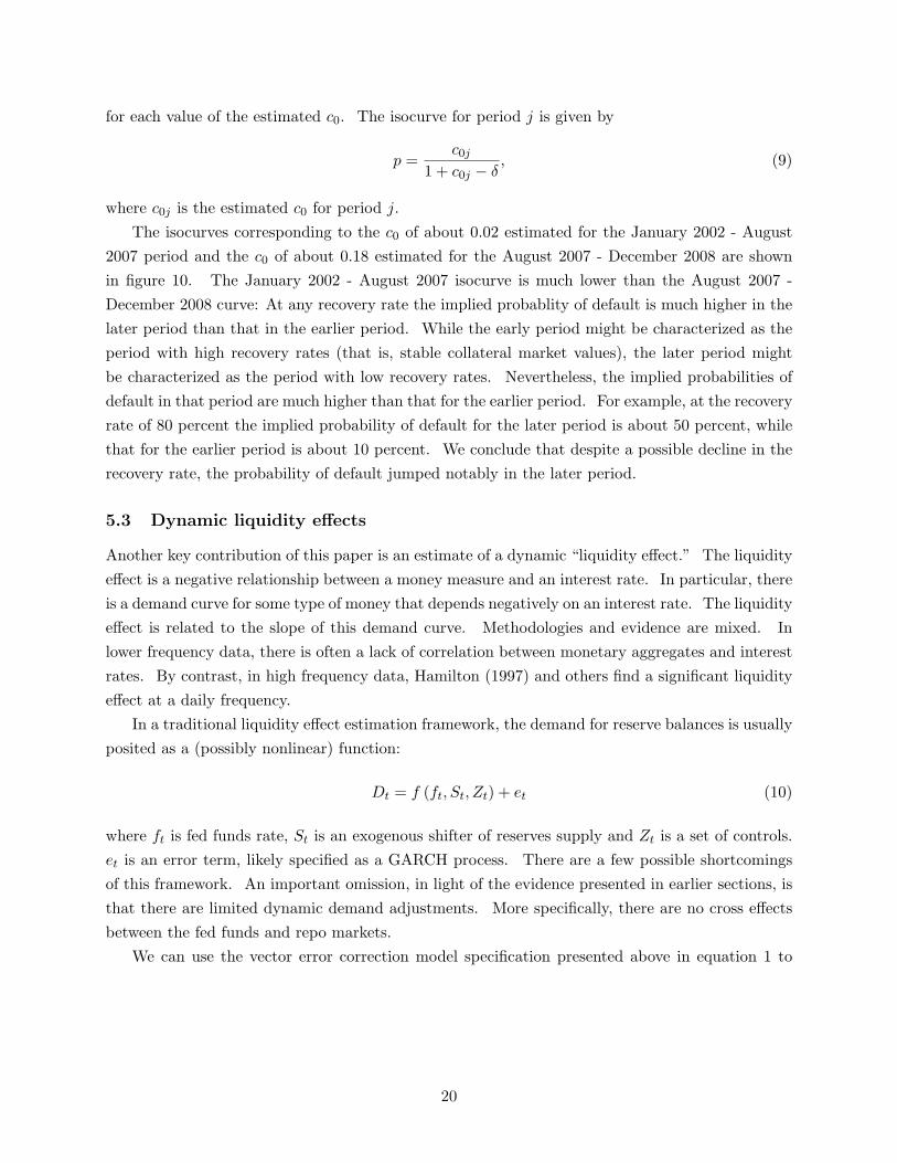
The isocurves corresponding to the c0 of about 0.02 estimated for the January 2002 - August

2007 period and the c0 of about 0.18 estimated for the August 2007 - December 2008 are shown

in figure 10. The January 2002 - August 2007 isocurve is much lower than the August 2007 -

December 2008 curve: At any recovery rate the implied probablity of default is much higher in the

later period than that in the earlier period. While the early period might be characterized as the

period with high recovery rates (that is, stable collateral market values), the later period might

be characterized as the period with low recovery rates. Nevertheless, the implied probabilities of

default in that period are much higher than that for the earlier period. For example, at the recovery

rate of 80 percent the implied probability of default for the later period is about 50 percent, while

that for the earlier period is about 10 percent. We conclude that despite a possible decline in the

recovery rate, the probability of default jumped notably in the later period.

5.3 Dynamic liquidity effects

Another key contribution of this paper is an estimate of a dynamic “liquidity effect.” The liquidity

effect is a negative relationship between a money measure and an interest rate. In particular, there

is a demand curve for some type of money that depends negatively on an interest rate. The liquidity

effect is related to the slope of this demand curve. Methodologies and evidence are mixed. In

lower frequency data, there is often a lack of correlation between monetary aggregates and interest

rates. By contrast, in high frequency data, Hamilton (1997) and others find a significant liquidity

effect at a daily frequency.

In a traditional liquidity effect estimation framework, the demand for reserve balances is usually

posited as a (possibly nonlinear) function:

Dt = f (ft, St, Zt) + et (10)

where ft is fed funds rate, St is an exogenous shifter of reserves supply and Zt is a set of controls.

et is an error term, likely specified as a GARCH process. There are a few possible shortcomings

of this framework. An important omission, in light of the evidence presented in earlier sections, is

that there are limited dynamic demand adjustments. More specifically, there are no cross effects

between the fed funds and repo markets.

We can use the vector error correction model specification presented above in equation 1 to

20

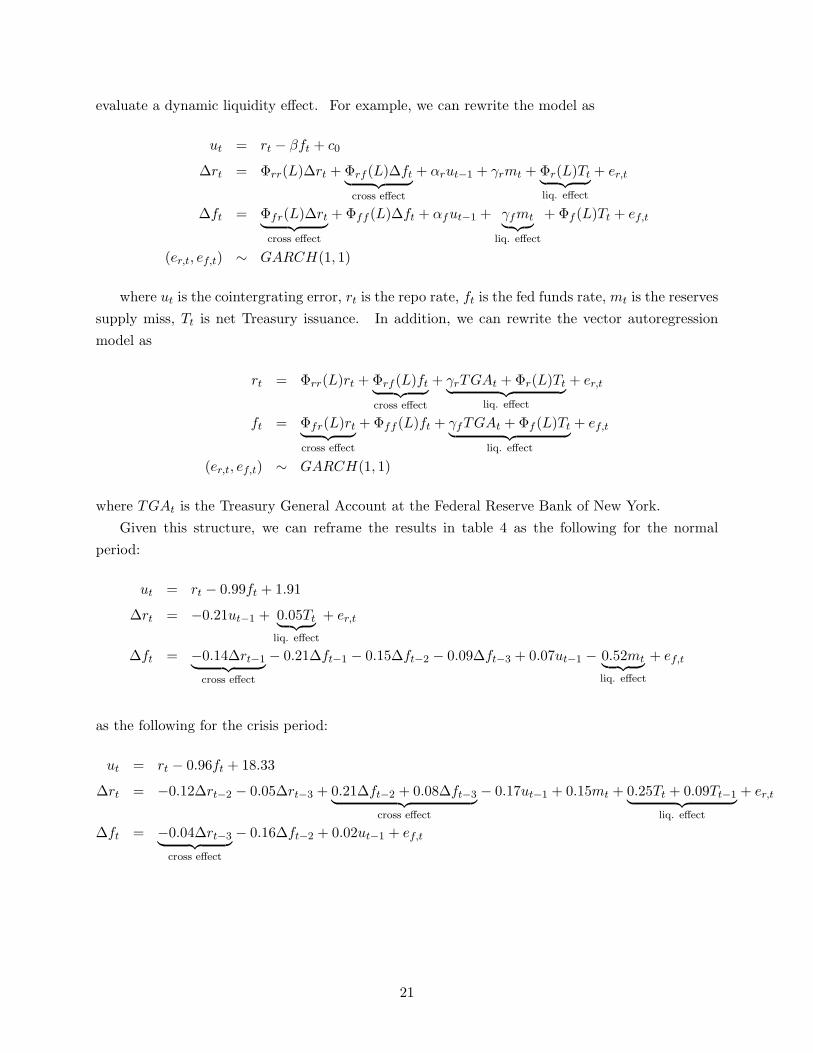
evaluate a dynamic liquidity effect. For example, we can rewrite the model as

ut = rt − βft + c0

∆rt = Φrr(L)∆rt +Φrf (L)∆ft︸ ︷︷ ︸

cross effect

+ αrut−1 + γrmt +Φr(L)Tt︸ ︷︷ ︸

liq. effect

+ er,t

∆ft = Φfr(L)∆rt︸ ︷︷ ︸

cross effect

+Φff (L)∆ft + αfut−1 + γfmt︸ ︷︷ ︸

liq. effect

+Φf (L)Tt + ef,t

(er,t, ef,t) ∼ GARCH(1, 1)

where ut is the cointergrating error, rt is the repo rate, ft is the fed funds rate, mt is the reserves

supply miss, Tt is net Treasury issuance. In addition, we can rewrite the vector autoregression

model as

rt = Φrr(L)rt +Φrf (L)ft︸ ︷︷ ︸

cross effect

+ γrTGAt +Φr(L)Tt︸ ︷︷ ︸

liq. effect

+ er,t

ft = Φfr(L)rt︸ ︷︷ ︸

cross effect

+Φff (L)ft + γfTGAt +Φf (L)Tt︸ ︷︷ ︸

liq. effect

+ ef,t

(er,t, ef,t) ∼ GARCH(1, 1)

where TGAt is the Treasury General Account at the Federal Reserve Bank of New York.

Given this structure, we can reframe the results in table 4 as the following for the normal

period:

ut = rt − 0.99ft + 1.91

∆rt = −0.21ut−1 + 0.05Tt︸ ︷︷ ︸

liq. effect

+ er,t

∆ft = −0.14∆rt−1︸ ︷︷ ︸

cross effect

− 0.21∆ft−1 − 0.15∆ft−2 − 0.09∆ft−3 + 0.07ut−1 − 0.52mt︸ ︷︷ ︸

liq. effect

+ ef,t

as the following for the crisis period:

ut = rt − 0.96ft + 18.33

∆rt = −0.12∆rt−2 − 0.05∆rt−3 + 0.21∆ft−2 + 0.08∆ft−3︸ ︷︷ ︸

cross effect

− 0.17ut−1 + 0.15mt + 0.25Tt + 0.09Tt−1︸ ︷︷ ︸

liq. effect

+ er,t

∆ft = −0.04∆rt−3︸ ︷︷ ︸

cross effect

− 0.16∆ft−2 + 0.02ut−1 + ef,t

21

and as the following for the “extended period”:

rt = 0.63rt−1 + 0.02rt−2 + 0.15rt−3 + 0.47ft−1 + 0.04ft−2 − 0.35ft−3︸ ︷︷ ︸

cross effect

+−0.01TGAt + 0.05Tt + 0.02Tt−1︸ ︷︷ ︸

liq. effect

+ er,t

ft = 0.12rt−1 + 0.13rt−3︸ ︷︷ ︸

cross effect

+ 1.05ft−1 − 0.41ft−2 + 0.01TGAt − 0.01Tt−1︸ ︷︷ ︸

liq. effect

+ ef,t

These parameter estimates are used in the exercises below that forecast the effect of large-

scale reverse repurchase agreements used to drain reserve balances on the effective rate. A key

implication of the results above should be highlighted, however. The results suggest that the

effect of Treasury issuance on repo rates is roughly unchanged, on net, over the entire sample.

In the normal period, repo rates moved down 5bp per $100B in net issuance. During the crisis,

this sensistivity jumped to 25bp per $100B in net issuance. However, the results suggest that in

the extended period, this sensitivity dropped back again to 5bp per $100B in net issuance. The

common magnitude of this result could imply that the parameter estimates for one period may

be able to be applied in a different one, despite the possibliity of fundamental changes in these

markets.

6 Forecasting the effect of reverse repurchase agreements on the

effective rate

We can use the estimates of the liquidity effect to forecast the effect of reverse repurchase agreements

on the effective rate. One of the measures currently undergoing operational tests for draining

reserves are reverse repurchase agreements with a wide set of counterparties; that is, a counterparty

list that includes primary dealers as well as other entities.26 The results presented above allow

us to evaluate how this program might affect money market interest rates. It is important to

recognize that large scale reverse repos could potentially have direct and indirect effects on both

the Treasury GC repo rate and the federal funds rate. Direct effects on Treasury GC repo would

be through collateral available to market participants. By contrast, direct effects on the federal

funds rate would likely be through the draining of reserve balances. However, consistent with the

results presented above, there would likely be cross, or indirect, effects between the repo rate and

the funds rate that could amplify some effects, outside of the direct effects of draining collateral or

reserve balances. In the exercises that follow, we set all factors other than those depicted here to

their sample-average levels in order to condition on relatively normal circumstances in the markets.

Overall, the results suggest that large-scale draining of reserve balances might exert weak up-

ward pressure on the federal funds and repo rates at high levels of balances, but should exert strong

upward pressure at lower levels. To illustrate this phenomenon, figure 6 shows the hypothetical

effects of draining nearly $1 trillion in total balances. Because demand for balances is likely non-

linear, we apply the parameter estimates from the December 2008 to June 2010 to evaluate the

26For more information on eligble counterparties, refer to http://www.newyorkfed.org/markets/rrp_counterparties.html.

22

effects of draining the first $900 billion in balances, and we use the parameter estimates from the

January 2002 to August 2007 to evaluate draining balances down to about $20 billion, close to the

average level of required operating balances, or the amount of balances that banks are required to

hold in order to satisfy reserve requirements as well as clearing needs.

As shown in the top two panels of figure 11, we assume two different patterns for draining

reserve balances. The first, depicted by the blue line in the top left panel, is a fast approach,

where $900 billion in balances is drained over the course of 10 days. The second, shown by the red

line, is a more gradual approach, where $900 billion is drained over 30 days. The former strategy

requires individual repo operations to be larger, while the latter relaxes this requirement. In both

scenarios, however, as shown in the top right panel, the cumulative effect on reserve balances is the

same.

The middle two panels show the effect of the draining on rates. As shown in the left panel,

repo rates initially climb about 30 basis points, before falling and reaching an equilbrium interest

rate that is about 5 basis points above the baseline. By contrast, the federal funds rate initially

climbs up to 55 basis points, before settling at a rate about 35 basis points above the baseline. The

peak rates are higher under scenario 1 than under scenario 2, but the equilibrium rates are the

same.

The bottom panel depicts the behavior of the spread between the federal funds rate. Because

the federal funds rate is driven up to a much higher level than the repo rate, the spread widens to

a fairly substantial 25 basis points.

The dynmaics for draining the final $80 billion in reserbe balances are slightly different. As

shown in figure 12, even though the total amount of collateral removed from the market is less, the

middle left panel shows that the effect on the repo rate is more substantial and persistent: repo

rates rise about 40 basis points and stay elevated. By contrast, the effect on the federal funds rate

is somewhat more limited, with rates increasing only about 15 basis points overall. The net effect

of these dynamics is to cause a narrowing of the spread, as shown in the bottom panel.

One caveat of these results is that they depend on the assumption that the relevant parameters

of the demand function will not change substantially from those that are estimated on past data.

Given the introduction of interest on reserves in the fall of 2008, there is some chance that demand

for reserve balances fundamentally changed since the early part of our sample – for example, since

2002. Still, we see scope for the relevance of this exercise, as it at least attempts to characterize

the dynamics that still exist, as well as the possibility of differences in demand for balances as the

level of balances approaches that of required operating balances.

7 Conclusion

Financial markets experienced remarkable changes over the financial crisis, and money markets

were no exception. This paper attempts to characterize the changes in these markets and to use

these characterizations to address situations that could occur should operations one day return to

23

“normal.” Along the way, we showed how the speed of monetary policy transmission changed

during the crisis; how banks were compensated for the possibility of default in the federal funds

market; and how the demand curve for reserve balances morphed over time.

In sum, our results suggest that monetary policy transmission still functioned through a good

part of the crisis. The link changed somewhat as reserve balances ballooned. Still our results

suggest that draining balances should help restore relationship. And, although we don not address

it specifically, our results are likely robust to the explicit modeling of interest on excess reserves.

References

[1] Barro, Robert J. 1976. “The Loan Market, Collateral, and Rates of Interest,” Journal of

Money, Credit, and Banking, vol. 8, no. 4, p. 439-456, November.

[2] Bartolini, Leonardo, Hilton, Spence, Sundaresan, Suresh, and Tonetti, Christopher. 2010.

“Collateral values by asset class: Evidence from Primary Securities Dealers,” Review of Fi-

nancial Studies, forthcoming.

[3] Brunnermeier, Markus and Pedersen, Lasse. 2009. “Market Liquidity and Funding Liquidity,”

Review of Financial Studies,” vol. 22, no. 6, p. 2201-2238.

[4] Coffey, Niall, Hrung, Warren B., and Sarkar, Asani. 2009. “Capital Constraints, Counterparty

Risk, and Deviation from Covered Interest Rate Parity,” Federal Reserve Bank of New York

Staff Report no. 393, September.

[5] Collin-Dufresne Pierre, Robert S. Goldstein, J. Spencer Martin 2001. “The Determinants of

Credit Spread Changes,” Journal of Finance, vol. 56, no. 6, p. 2177-2207.

[6] Duffie, Darrell. 1996. “Special Repo Rates,” Journal of Finance, vol. 51, no 2, p. 493-526,

June.

[7] Engle, Robert F. and Granger, Clive W. 1987. “Cointegration and Error-Correction Model:

Representation, Estimation, and Testing,” Econometrica, vol. 55, no. 2, p. 251-276.

[8] Engle, Robert F. and Kroner, Kenneth F. 1995. “Multivariate Simultaneous Generalized

ARCH,” Econometric Theory, vol. 11, no. 1, p. 122-150.

[9] Federal Reserve Bank of New York. 2009. Domestic Open Market Operations during 2008,

January.

[10] Federal Reserve Bank of New York. 2010. “Tri-party Repo Infrastructure Reform,” May 17.

[11] Fisher, Mark. 2002. “Special repo rates: An introduction,” Economic Review, Federal Reserve

Bank of Atlanta, Second quarter.

24

[12] Fleming, Michael, and Garbade, Kenneth. 2005. “Explaining Settlement Fails,” Current Issues

in Economics and Finance, Federal Reserve Bank of New York, vol. 11, no. 9, September.

[13] Fleming, Michael, Hrung, Warren, and Keane, Frank. 2008. “Repo Market Effects of the

Term Securities Lending Facility,” Federal Reserve Bank of New York Staff Report no. 426,

January 2010.

[14] Friedman, Milton, and Schwartz, Anna J. 1963. A Monetary History of the United States.

Cambridge: NBER.

[15] Furfine, Craig. 1999. “The Microstructure of the Federal Funds Market,” Financial Markets,

Institutions, and Instruments, vol. 8, no. 5, p. 24-44.

[16] Griffiths, Mark D. and Winters, Drew B. 1997. “The effect of Federal Reserve accounting rules

on the equilibrium level of overnight repo rates,” Journal of Business Finance and Accounting,

vol. 24, no. 6, p. 815-832, July.

[17] Gorton, Gary. 2010. “Questions and Answers about the Financial Crisis,” prepared for the

U.S. Financial Crisis Inquiry Commission, February 20.

[18] Hamilton, James. 1996. “The daily market for federal funds,” Journal of Political Economy,

vol. 104, no. 1, p. 26-56.

[19] Hamilton, James. 1997. “Measuring the liquidity effect,” American Economic Review, vol.

87, no. 1, p. 80-97, March.

[20] Happ, Scott. 1986. “The behavior of rates on federal funds and repurchase agreements,” The

American Economist, vol. 30, no. 2, p. 22-32, Fall.

[21] Johansen, Soren. 1995. “Identifying restrictions of liner equations with applications to si-

multaneous equations and cointegration,” Journal of Econometrics, vol. 69 (1), p. 111-132,

September.

[22] Krishnamurthy, Arvind. 2002. “The bond/old bond spread,” Journal of Financial Economics,

vol. 66, p. 463-506.

[23] Lutkepohl, Helmut. 2007. New Introduction to Multiple Time Series Analysis. Berlin:

Springer-Verlag.

[24] Simmons, Edward C. 1954. “Sales of Government Securities to Federal Reserve Banks Under

Repurchase Agreements,” The Journal of Finance, vol. 9, no. 1, p. 23-40.

[25] Stigum, Marcia, and Credenzi, Anthony. 2007. The Money Market. McMillian: New York.

[26] Thornton, Daniel L. 2004. “Tests of the expectations hypothesis: Resolving some anomalies

when the short-term rate is the federal funds rate,” Journal of Banking and Finance, vol. 29,

p. 2541-2556.

25

[Figure 1 about here.]

[Figure 2 about here.]

[Figure 3 about here.]

[Figure 4 about here.]

[Figure 5 about here.]

[Figure 6 about here.]

[Table 1 about here.]

[Table 2 about here.]

[Table 3 about here.]

[Table 4 about here.]

[Figure 7 about here.]

[Figure 8 about here.]

[Table 5 about here.]

[Table 6 about here.]

[Table 7 about here.]

[Figure 9 about here.]

[Figure 10 about here.]

[Figure 11 about here.]

[Figure 12 about here.]

26

List of Figures

1 Federal funds and Treasury GC repo . . . . . . . . . . . . . . . . . . . . . . . . 282 Spread between federal funds and Treasury GC repo . . . . . . . . . . . . . 293 Primary dealers repurchase agreement volume . . . . . . . . . . . . . . . . . . 304 Federal funds market volume . . . . . . . . . . . . . . . . . . . . . . . . . . . . . 315 Federal funds and repos at commercial banks: Quarterly . . . . . . . . . . . 326 Federal funds and repos at commercial banks: Weekly . . . . . . . . . . . . 337 Share of repo and federal funds, by bank asset size . . . . . . . . . . . . . . . 348 Net Treasury issuance and Treasury General Account (TGA) balance . . . 359 Speeds of adjustment . . . . . . . . . . . . . . . . . . . . . . . . . . . . . . . . . . 3610 P-δ isocurves . . . . . . . . . . . . . . . . . . . . . . . . . . . . . . . . . . . . . . . 3711 Draining the first $900 billion . . . . . . . . . . . . . . . . . . . . . . . . . . . . 3812 Draining the second $80 billion . . . . . . . . . . . . . . . . . . . . . . . . . . . 39

27

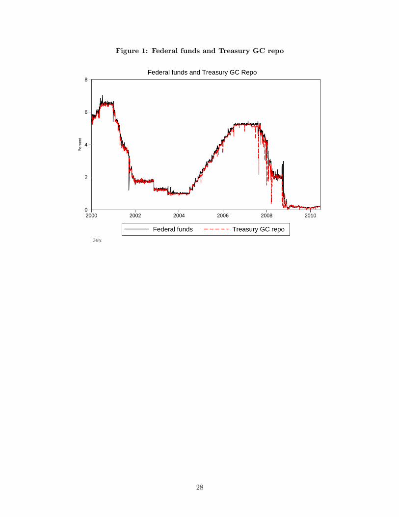
Figure 1: Federal funds and Treasury GC repo

0

2

4

6

8P

erce

nt

2000 2002 2004 2006 2008 2010

Federal funds Treasury GC repo

Daily.

Federal funds and Treasury GC Repo

28

Figure 2: Spread between federal funds and Treasury GC repo

−50

0

50

100

150

200

250

Bas

is p

oint

s

2000 2002 2004 2006 2008 2010Daily.

Federal Funds−Overnight GC Repo Spread

29

Figure 3: Primary dealers repurchase agreement volume

0

200

400

600

800

1000

$ bi

llion

s

1995 2000 2005 2010

Total Treasury

Volume of Treasury, Agency Debt, and MBS Repos with Inter−Dealer Brokers

0

200

400

600

800

1000

$ bi

llion

s

1995 2000 2005 2010

Total Treasury

Source. FR2004.

Volume of Treasury, Agency Debt, and MBS Repos with Others

30

Figure 4: Federal funds market volume

0

100

200

300

400

500$

billi

ons

1998 2000 2002 2004 2006 2008 2010

Note: Identified in Fedwire transaction data using Furfine (1999) algorithm.

Federal funds volume

31

Figure 5: Federal funds and repos at commercial banks: Quarterly

100

150

200

250

300$

billi

ons

Jan 2002 Jan 2004 Jan 2006 Jan 2008 Jan 2010

Federal Funds Purchased

1

1.5

2

2.5

3

3.5

4

perc

ent

Jan 2002 Jan 2004 Jan 2006 Jan 2008 Jan 2010

Percent of Liabilities

50

100

150

200

250

$ bi

llion

s

Jan 2002 Jan 2004 Jan 2006 Jan 2008 Jan 2010

Federal Funds Sold

.5

1

1.5

2

2.5

3

perc

ent

Jan 2002 Jan 2004 Jan 2006 Jan 2008 Jan 2010

Percentage of Assets

100

120

140

160

180

200

220

240

260

280

300

320

$ bi

llion

s

Jan 2002 Jan 2004 Jan 2006 Jan 2008 Jan 2010

Securities Purchased to Resell

1.4

1.6

1.8

2

2.2

2.4

2.6

2.8

3

perc

ent

Jan 2002 Jan 2004 Jan 2006 Jan 2008 Jan 2010

Percent of Assets

260

280

300

320

340

360

380

400

420

440

$ bi

llion

s

Jan 2002 Jan 2004 Jan 2006 Jan 2008 Jan 2010

Securities Sold to be Repurchased

3.84

4.24.44.64.8

55.25.45.65.8

6

perc

ent

Jan 2002 Jan 2004 Jan 2006 Jan 2008 Jan 2010

Percent of Liabilities

32

Figure 6: Federal funds and repos at commercial banks: Weekly

50

100

150

200$

billi

ons

Jan 1998 Jan 2000 Jan 2002 Jan 2004 Jan 2006 Jan 2008 Jan 2010

Federal Funds and Reverse RPs with Banks

.5

1

1.5

2

2.5

perc

ent

Jan 1998 Jan 2000 Jan 2002 Jan 2004 Jan 2006 Jan 2008 Jan 2010

Percentage of Assets

100

150

200

250

300

350

$ bi

llion

s

Jan 1998 Jan 2000 Jan 2002 Jan 2004 Jan 2006 Jan 2008 Jan 2010

Federal funds and reverse RPs with nonbanks

1.5

2

2.5

3

3.5

perc

ent

Jan 1998 Jan 2000 Jan 2002 Jan 2004 Jan 2006 Jan 2008 Jan 2010

Percentage of Assets

33

Figure 7: Share of repo and federal funds, by bank asset size

0

.2

.4

.6

.8

1

Sha

re

Jan 2002 Jan 2004 Jan 2006 Jan 2008 Jan 2010

Top 10 11−100

101−1000 Not in 1−1000

Securities sold to be repurchased

0

.2

.4

.6

.8

1

Sha

re

Jan 2002 Jan 2004 Jan 2006 Jan 2008 Jan 2010

Top 10 11−100

101−1000 Not in 1−1000

Federal funds sold

0

.2

.4

.6

.8

1

Sha

re

Jan 2002 Jan 2004 Jan 2006 Jan 2008 Jan 2010

Top 10 11−100

101−1000 Not in 1−1000

Securities purchased to be resold

0

.2

.4

.6

.8

1

Sha

re

Jan 2002 Jan 2004 Jan 2006 Jan 2008 Jan 2010

Top 10 11−100

101−1000 Not in 1−1000

Federal funds purchased

34

Figure 8: Net Treasury issuance and Treasury General Account (TGA) balance

−50

050

$ bi

llion

s

2002 2004 2006 2008Date

Net Treasury issuance TGA

−50

050

100

150

200

$ bi

llion

s

2008 2009 2010 2011Date

Net Treasury issuance TGA

35

Figure 9: Speeds of adjustment

- 0 . 8- 0 . 7- 0 . 6- 0 . 5- 0 . 4- 0 . 3- 0 . 2- 0 . 10 . 0

B asi spoi nt s

O v e r n i g h t T r e a s u r y G C R e p o R a t eJ a n 0 2 - A u g 0 7A u g 0 7 - D e c 0 8

- 1 . 0- 0 . 9 1 2 3 4 5 6 7 8 9D a y s

- 0 . 8- 0 . 7- 0 . 6- 0 . 5- 0 . 4- 0 . 3- 0 . 2- 0 . 10 . 0

B asi spoi nt s

F e d e r a l F u n d s R a t e

J a n 0 2 - A u g 0 7A u g 0 7 - D e c 0 8- 1 . 0- 0 . 9 1 2 3 4 5 6 7 8 9D a y s36

Figure 10: P-δ isocurves

2 0 %3 0 %4 0 %5 0 %6 0 %7 0 %8 0 %9 0 %1 0 0 %

P rob abili t yofd ef aul t

P - d e l t a i s o c u r v e sA u g 0 7 - D e c 0 8J a n 0 2 - A u g 0 7

0 %1 0 % 0 % 1 0 % 2 0 % 3 0 % 4 0 % 5 0 % 6 0 % 7 0 % 8 0 % 9 0 % 1 0 0 %R e c o v e r y r a t e

37

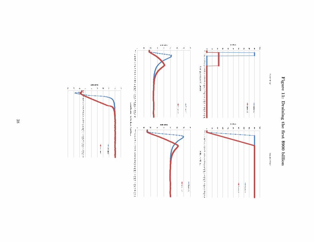
Figure

11:Dra

iningth

efirst

$900billio

n

20 30 4 0 5 0 60 7 0 80 90 1 00$ b i l l io n sReverseRepos

Scenario1Scenario20 1 0171 31 9253 13 743495 561677 37 9859 19 71 0 31 0 91 1 51 211 271 3 31 3 91 451 5 11 5 71 631 691 7 51 811 871 9 31 9 9 200 300 4 00 5 00 600 7 00 800 900 1 000$ b i l l io n s

CumulativeDrainScenario1Scenario2

0 1 00171 31 9253 13 743495 561677 37 9859 19 71 0 31 0 91 1 51 211 271 3 31 3 91 451 5 11 5 71 631 691 7 51 811 871 9 31 9 9

20 30 4 0 5 0 60 7 0 80ba s i s p o in t sOvernightTreasuryGCreporateScenario1Scenario2

0 10171 31 9253 13 743495 561677 37 9859 19 71 0 31 0 91 1 51 211 271 3 31 3 91 451 5 11 5 71 631 691 7 51 811 871 9 31 9 9 20 30 4 0 5 0 60 7 0 80ba s i s p o in t sFederalFundsrateScenario1Scenario2

0 10171 31 9253 13 743495 561677 37 9859 19 71 0 31 0 91 1 51 211 271 3 31 3 91 451 5 11 5 71 631 691 7 51 811 871 9 31 9 9

-5 0 5 1 0 15 20 25 30171 31 9253 13 743495 561677 37 9859 19 71 0 31 0 91 1 51 2 11 2 71 3 31 3 91 4 51 5 11 5 71 6 31 6 91 7 51 8 11 8 71 9 31 9 9ba s i s p o in t s SpreadbetweenFedFundsandRepoRatesScenario1Scenario2

- 15 - 1 0

38

Figure

12:Dra

iningth

esecond

$80billio

n

9ReverseRepos

7 8Scenario1Scenario2

4 5 6$ b i l l io n s2 30 11471 01 31 61 92 225 283 13 43 74 04 34 64 95 25 55 86 16 46 77 07 37 67 98 28 58 89 19 49 71 0 0 90CumulativeDrain

7 0 80Scenario1

40 5 0 60$ b i l l io n sScenario2

20 300 101471 01 31 61 92 225 283 13 43 74 04 34 64 95 25 55 86 16 46 77 07 37 67 98 28 58 89 19 49 71 0 080 OvernightTreasuryGCreporate60 7 040 5 0ba s i s p o in t s

Scenario120 30

Scenario20 101471 01 31 61 92 225 283 13 43 74 04 34 64 95 25 55 86 16 46 77 07 37 67 98 28 58 89 19 49 71 0 0 80

FederalFundsrateScenario1

60 7 0Scenario1Scenario2

40 5 0ba s i s p o in t s20 300 101471 01 31 61 92 225 283 13 43 74 04 34 64 95 25 55 86 16 46 77 07 37 67 98 28 58 89 19 49 71 0 030 SpreadbetweenFedFundsandRepoRates20

Scenario1Scenario20 101471 01 31 61 9 2 225 283 13 43 74 04 34 64 95 25 55 86 16 46 77 07 37 67 98 28 58 89 19 49 71 0 0

ba s i s p o in t s- 20 - 10- 3039

List of Tables

1 Augmented Dickey-Fuller tests . . . . . . . . . . . . . . . . . . . . . . . . . . . . 412 Johansen cointegration tests: federal funds and repo . . . . . . . . . . . . . . 423 Granger causality tests . . . . . . . . . . . . . . . . . . . . . . . . . . . . . . . . . 434 Results highlights . . . . . . . . . . . . . . . . . . . . . . . . . . . . . . . . . . . . 445 Normal times: January 2002-August 2007 . . . . . . . . . . . . . . . . . . . . 456 Crisis: August 2007-December 2008 . . . . . . . . . . . . . . . . . . . . . . . . 467 Extended period: December 2008-June 2010 . . . . . . . . . . . . . . . . . . . 47

40

Table 1: Augmented Dickey-Fuller tests

Federal funds Repo NJanuary 2002 - August 2007 1.054 1.068 1399

10 6August 2007 - December 2008 -0.769 2.345 331

3 1December 2008 - June 2010 -6.513∗∗ -5.076∗∗ 385

2 1

Lag length below test statistic.∗∗ Reject hypothesis of a unit root at the 5 percent confidence level.

41

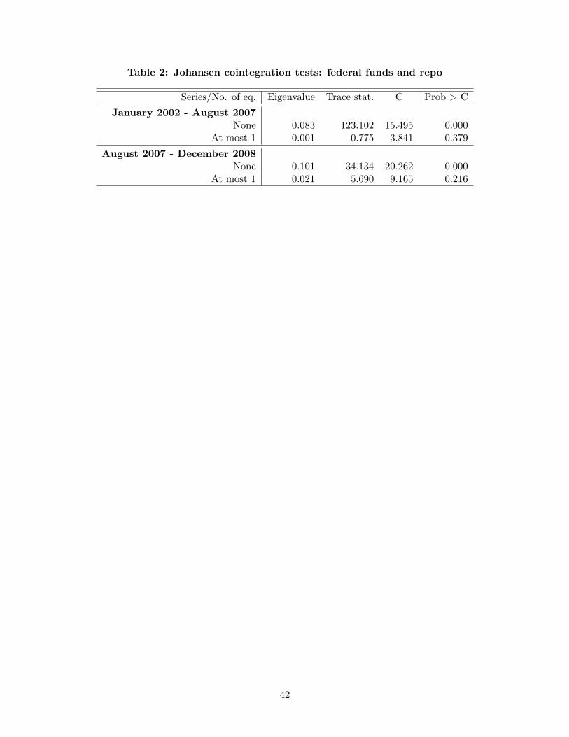
Table 2: Johansen cointegration tests: federal funds and repo

Series/No. of eq. Eigenvalue Trace stat. C Prob > C

January 2002 - August 2007None 0.083 123.102 15.495 0.000

At most 1 0.001 0.775 3.841 0.379

August 2007 - December 2008None 0.101 34.134 20.262 0.000

At most 1 0.021 5.690 9.165 0.216

42

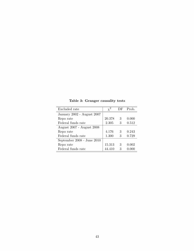
Table 3: Granger causality tests

Excluded rate χ2 DF Prob.

January 2002 - August 2007Repo rate 20.378 3 0.000Federal funds rate 2.305 3 0.512

August 2007 - August 2008Repo rate 4.176 3 0.243Federal funds rate 1.300 3 0.729

September 2008 - June 2010Repo rate 15.313 3 0.002Federal funds rate 44.410 3 0.000

43

Table 4: Results highlightsS a m p l e p e r i o d s J a n . 2 0 0 2 - A u g . 2 0 0 7 A u g . 2 0 0 7 - D e c . 2 0 0 8 D e c . 2 0 0 8 - J u n . 2 0 1 0E c o n o m e t r i c m o d e l V E C / G A R C H V E C / G A R C H V A R / G A R C HC o i n t e g r a t i n g v e c t o rC o n s t a n t - 1 . 9 1 3 - 1 8 . 3 2 7 N AS l o p e 0 . 9 8 7 0 . 9 6 2 N AD y n a m i c e q u a t i o nR e p o e q u a t i o nS p e e d o f a d j u s t m e n t - 0 . 2 0 9 - 0 . 1 7 4 N AF a c t o r m i s s N S 0 . 1 4 8 N AN e t i s s u a n c e 0 . 0 4 9 0 . 2 5 4 0 . 0 4 7L a g o f n e t i s s u a n c e N S 0 . 0 9 4 0 . 0 1 5L S A P N A N A N ST G A N A N A - 0 . 0 0 5R ^ 2 0 . 3 2 7 0 . 2 6 0 0 . 8 5 8D W 2 . 1 9 3 1 . 7 6 4 2 . 1 1 7

E s t i m a t i o n r e s u l t s

D y n a m i c e q u a t i o nF e d f u n d s e q u a t i o nS p e e d o f a d j u s t m e n t 0 . 0 6 6 0 . 0 1 7 N AF a c t o r m i s s - 0 . 5 2 0 N S N AN e t i s s u a n c e N S N S N SL a g o f n e t i s s u a n c e N S N S - 0 . 0 1 4L S A P N A N A - 0 . 0 4 2T G A N A N A 0 . 0 1 1R ^ 2 0 . 3 2 8 0 . 1 1 4 0 . 7 1 2D W 1 . 9 3 8 2 . 2 3 3 2 . 2 8 6N u m b e r o f o b s e r v a t i o n s 1 4 1 0 3 3 0 3 8 5T o t a l b a l a n c e sM e d i a n , $ b i l l i o n s 2 0 1 7 9 1 3R a n g e , $ b i l l i o n s 1 0 … 4 4 9 … 6 6 0 5 9 8 … 1 2 4 944

Table 5: Normal times: January 2002-August 2007C o e f f i c i e n t S t d . e r r o r Z - s t a t C o e f f i c i e n t S t d . e r r o r Z - s t a tC o i n t e g r a t i n g t e r m - 0 . 2 0 9 0 . 0 4 0 - 5 . 2 0 4 0 . 0 6 6 0 . 0 2 7 2 . 4 7 7D ( r e p o ( - 1 ) ) - 0 . 1 8 3 0 . 1 1 2 - 1 . 6 3 2 - 0 . 1 4 4 0 . 0 5 1 - 2 . 8 3 9D ( r e p o ( - 2 ) ) - 0 . 1 0 1 0 . 0 7 2 - 1 . 3 8 9 - 0 . 0 6 2 0 . 0 7 0 - 0 . 8 8 8D ( r e p o ( - 3 ) ) - 0 . 0 5 9 0 . 0 6 0 - 0 . 9 8 7 - 0 . 0 3 7 0 . 0 4 9 - 0 . 7 5 4D ( f f e f f ( 1 ) ) 0 0 2 7 0 1 0 9 0 2 4 6 0 2 1 0 0 0 5 4 3 8 9 6T r e a s u r y G C R e p o F e d e r a l f u n d s

D ( f f e f f ( - 1 ) ) 0 . 0 2 7 0 . 1 0 9 0 . 2 4 6 - 0 . 2 1 0 0 . 0 5 4 - 3 . 8 9 6D ( f f e f f ( - 2 ) ) 0 . 0 2 1 0 . 1 0 9 0 . 1 9 6 - 0 . 1 5 2 0 . 0 6 9 - 2 . 2 1 4D ( f f e f f ( - 3 ) ) 0 . 0 1 4 0 . 0 6 4 0 . 2 2 6 - 0 . 0 9 3 0 . 0 3 9 - 2 . 3 8 9M P d a y 1 1 . 4 5 5 2 . 0 2 3 0 . 7 1 9 - 0 . 4 6 7 2 . 6 8 2 - 0 . 1 7 4M P d a y 2 - 1 . 8 1 4 1 . 8 3 3 - 0 . 9 8 9 - 4 . 3 5 5 2 . 4 5 0 - 1 . 7 7 8M P d a y 5 1 . 5 1 8 2 . 0 2 0 0 . 7 5 1 - 0 . 6 8 9 2 . 0 6 8 - 0 . 3 3 3M P d a y 6 - 0 . 6 1 9 1 . 6 9 2 - 0 . 3 6 6 - 3 . 1 2 1 2 . 6 9 4 - 1 . 1 5 8d a y 6 0 6 9 6 9 0 3 6 6 3 6 9 5 8M P d a y 7 - 0 . 1 0 8 1 . 4 6 2 - 0 . 0 7 4 - 2 . 4 3 5 2 . 6 1 4 - 0 . 9 3 1M P d a y 8 0 . 7 9 6 1 . 6 5 0 0 . 4 8 3 - 0 . 7 4 2 2 . 6 0 6 - 0 . 2 8 5M P d a y 9 - 0 . 4 8 3 2 . 6 5 7 - 0 . 1 8 2 - 2 . 9 1 4 2 . 5 9 7 - 1 . 1 2 2M P d a y 1 2 1 . 3 5 6 1 . 8 2 9 0 . 7 4 1 - 1 . 1 4 1 2 . 5 9 1 - 0 . 4 4 0M P d a y 1 3 - 1 . 2 8 8 1 . 8 9 9 - 0 . 6 7 8 - 5 . 9 9 1 2 . 6 5 2 - 2 . 2 5 9M P d a y 1 4 - 0 . 5 4 0 1 . 7 4 7 - 0 . 3 0 9 - 2 . 2 4 0 2 . 5 9 3 - 0 . 8 6 4M i d t h 4 6 4 1 1 6 2 6 2 8 5 4 4 7 6 5 0 7 0 2 6 7 8 6M i d - m o n t h 4 . 6 4 1 1 . 6 2 6 2 . 8 5 4 4 . 7 6 5 0 . 7 0 2 6 . 7 8 6M o n t h - e n d 2 . 7 8 2 1 . 5 2 7 1 . 8 2 1 3 . 4 9 5 0 . 5 3 1 6 . 5 7 92 5 t h o f m o n t h 0 . 7 6 9 0 . 8 4 9 0 . 9 0 6 4 . 1 7 7 0 . 5 5 4 7 . 5 3 5Q u a r t e r - e n d - 5 . 8 6 8 3 0 . 2 6 5 - 0 . 1 9 4 1 1 . 0 6 1 3 . 0 8 2 3 . 5 8 9Y e a r - e n d 1 . 2 8 4 1 1 . 6 2 5 0 . 1 1 0 - 1 1 . 6 3 0 1 2 . 0 7 0 - 0 . 9 6 4D ( t a r g e t ) 7 . 0 6 3 1 2 . 9 9 2 0 . 5 4 4 9 . 8 3 9 2 7 . 0 0 3 0 . 3 6 4D ( f e d f u n d s v o l ) 0 . 0 5 5 0 . 1 0 3 0 . 5 3 1 0 . 0 9 7 0 . 0 4 3 2 . 2 2 8D ( f e d f u n d s v o l ) 0 . 0 5 5 0 . 1 0 3 0 . 5 3 1 0 . 0 9 7 0 . 0 4 3 2 . 2 2 8F a c t o r m i s s - 0 . 0 5 6 0 . 1 6 6 - 0 . 3 3 8 - 0 . 5 2 0 0 . 1 7 6 - 2 . 9 5 0D ( n u m s e l l e r s ) 0 . 0 0 6 0 . 0 0 4 1 . 5 9 3 - 0 . 0 0 4 0 . 0 0 8 - 0 . 5 0 8D ( G S E f u n d s s o l d ) - 0 . 1 0 0 0 . 0 3 3 - 3 . 0 3 1 - 0 . 0 7 6 0 . 0 3 1 - 2 . 4 5 3D ( L i b o r - O I S ) 0 . 0 4 7 0 . 1 2 3 0 . 3 8 6 - 0 . 0 5 0 0 . 2 1 7 - 0 . 2 2 9D ( R i s k - w e i g h t e d c a p i t a l r a t i o ) 5 . 2 7 1 4 3 . 4 1 9 0 . 1 2 1 1 3 . 8 8 6 1 5 . 9 2 4 0 . 8 7 2D ( T r e a s u r y r e p o f a i l s ) - 0 . 0 1 0 0 . 0 1 7 - 0 . 5 7 3 - 0 . 0 0 1 0 . 0 1 3 - 0 . 0 9 5N e t T r e a s u r y i s s u a n c e 0 . 0 4 9 0 . 0 1 6 3 . 0 7 7 0 . 0 1 2 0 . 0 1 3 0 . 9 1 0N e t T r e a s u r y i s s u a n c e ( - 1 ) 0 . 0 1 7 0 . 0 3 2 0 . 5 2 0 - 0 . 0 2 0 0 . 0 1 7 - 1 . 1 7 0O v e r n i g h t s e c u r i t i e s l e n d i n g - 0 . 0 1 0 0 . 0 5 5 - 0 . 1 7 4 - 0 . 0 2 9 0 . 0 7 5 - 0 . 3 8 1Y i e l d c u r v e s l o p e 0 . 0 4 3 0 . 0 4 4 0 . 9 7 8 - 0 . 1 2 3 0 . 0 4 2 - 2 . 9 3 2D e a l e r b o o k 0 . 1 1 4 0 . 8 1 6 0 . 1 4 0 0 . 1 6 3 0 . 5 4 4 0 . 2 9 9R - s q u a r e d 0 . 3 4 4 0 . 3 4 4D u r b i n - W a t s o n 2 . 1 9 0 1 . 9 4 0D u r b i n - W a t s o n 2 . 1 9 0 1 . 9 4 0N 1 4 0 645

Table 6: Crisis: August 2007-December 2008C o e f f i c i e n t S t d . e r r o r Z - s t a t C o e f f i c i e n t S t d . e r r o r Z - s t a tC o i n t e g r a t i n g t e r m - 0 . 1 7 4 0 . 0 4 2 - 4 . 1 3 0 0 . 0 1 7 0 . 0 0 4 3 . 9 1 0D ( r e p o ( - 1 ) ) 0 . 0 0 2 0 . 0 0 0 4 . 9 9 1 - 0 . 0 2 0 0 . 0 2 2 - 0 . 8 8 6D ( r e p o ( - 2 ) ) - 0 . 1 2 4 0 . 0 2 8 - 4 . 3 8 3 - 0 . 0 2 0 0 . 0 2 2 - 0 . 9 1 4D ( r e p o ( - 3 ) ) - 0 . 0 4 6 0 . 0 1 1 - 4 . 1 8 8 - 0 . 0 3 6 0 . 0 2 1 - 1 . 6 7 5D ( f f e f f ( - 1 ) ) 0 . 0 0 1 0 . 0 0 1 1 . 7 8 0 0 . 0 4 3 0 . 0 6 6 0 . 6 4 1D ( f f e f f ( - 2 ) ) 0 . 2 1 3 0 . 0 4 7 4 . 5 6 0 - 0 . 1 6 4 0 . 0 6 0 - 2 . 7 1 7D ( f f e f f ( - 3 ) ) 0 . 0 8 5 0 . 0 1 4 5 . 8 7 5 - 0 . 0 1 0 0 . 0 0 8 - 1 . 2 3 6M P d a y 1 - 1 9 5 . 9 6 5 9 . 9 6 2 - 1 9 . 6 7 2 - 1 1 0 . 8 2 9 2 2 . 5 7 1 - 4 . 9 1 0M P d a y 2 - 1 9 3 . 7 8 0 1 0 . 3 5 5 - 1 8 . 7 1 3 - 1 1 7 . 9 4 4 2 3 . 2 5 2 - 5 . 0 7 2M P d a y 5 - 1 9 7 . 8 5 0 1 0 . 2 7 1 - 1 9 . 2 6 4 - 1 1 4 . 1 5 3 2 2 . 4 1 2 - 5 . 0 9 3M P d a y 6 - 2 0 1 . 3 7 3 1 0 . 9 2 8 - 1 8 . 4 2 6 - 1 1 9 . 8 5 0 2 3 . 3 8 1 - 5 . 1 2 6M P d a y 7 - 1 9 8 . 7 3 0 1 0 . 6 5 8 - 1 8 . 6 4 5 - 1 1 4 . 4 1 8 2 3 . 0 4 4 - 4 . 9 6 5M P d a y 8 - 1 9 5 . 9 6 0 1 0 . 2 0 0 - 1 9 . 2 1 2 - 1 1 6 . 0 3 5 2 2 . 7 3 7 - 5 . 1 0 3M P d a y 9 - 2 0 1 . 6 9 9 1 0 . 4 6 3 - 1 9 . 2 7 7 - 1 1 8 . 8 1 3 2 2 . 6 4 0 - 5 . 2 4 8M P d a y 1 2 - 1 9 5 . 4 4 1 1 0 . 4 3 2 - 1 8 . 7 3 5 - 1 1 6 . 0 7 6 2 2 . 5 4 4 - 5 . 1 4 9M P d a y 1 3 - 2 0 0 . 9 1 1 1 0 . 4 4 2 - 1 9 . 2 4 1 - 1 1 5 . 9 5 0 2 2 . 6 3 8 - 5 . 1 2 2M P d a y 1 4 - 2 0 0 . 3 2 0 1 0 . 4 6 1 - 1 9 . 1 4 9 - 1 1 3 . 3 7 0 2 2 . 4 1 7 - 5 . 0 5 7M i d - m o n t h - 1 . 6 1 0 0 . 0 8 9 - 1 8 . 1 7 3 - 0 . 3 0 5 0 . 0 5 8 - 5 . 2 2 5M o n t h - e n d - 4 . 2 5 6 5 . 6 1 7 - 0 . 7 5 8 4 . 7 8 3 4 . 1 2 9 1 . 1 5 82 5 t h o f m o n t h - 6 . 4 8 3 3 . 1 0 4 - 2 . 0 8 9 1 0 . 9 9 8 2 . 6 9 1 4 . 0 8 7Q u a r t e r - e n d - 3 7 . 4 1 3 7 . 4 7 2 - 5 . 0 0 7 2 0 . 6 1 8 8 . 5 1 0 2 . 4 2 3Y e a r - e n d - 1 3 3 . 0 0 1 7 . 4 3 8 - 1 7 . 8 8 2 - 8 3 . 9 9 1 1 5 . 4 6 8 - 5 . 4 3 0D ( t a r g e t ) 1 . 0 3 1 0 . 0 5 3 1 9 . 2 9 1 0 . 5 3 8 0 . 0 8 3 6 . 5 1 0D ( f e d f u n d s v o l ) - 0 . 1 1 8 0 . 0 0 9 - 1 3 . 0 6 7 0 . 0 4 7 0 . 0 1 6 3 . 0 5 5F a c t o r m i s s 0 . 1 4 8 0 . 0 6 9 2 . 1 3 8 0 . 0 1 8 0 . 1 0 9 0 . 1 6 5D ( n u m s e l l e r s ) 0 . 0 8 9 0 . 0 4 0 2 . 2 0 3 - 0 . 0 8 2 0 . 0 4 3 - 1 . 9 1 7D ( G S E f u n d s s o l d ) - 0 . 1 5 9 0 . 0 7 5 - 2 . 1 0 8 0 . 1 2 0 0 . 0 7 6 1 . 5 7 6D ( L i b o r - O I S ) - 0 . 3 7 3 0 . 1 6 0 - 2 . 3 2 6 0 . 2 4 1 0 . 1 1 2 2 . 1 4 6D ( R i s k - w e i g h t e d c a p i t a l r a t i o ) 1 4 5 . 5 2 7 2 7 . 8 0 2 5 . 2 3 4 - 1 8 2 . 9 6 4 6 4 . 6 0 6 - 2 . 8 3 2D ( T r e a s u r y r e p o f a i l s ) 0 . 0 3 3 0 . 0 0 6 5 . 8 8 8 - 0 . 0 0 4 0 . 0 0 3 - 1 . 2 3 1N e t T r e a s u r y i s s u a n c e 0 . 2 5 4 0 . 0 6 5 3 . 9 1 6 0 . 0 4 9 0 . 0 4 5 1 . 0 9 8N e t T r e a s u r y i s s u a n c e ( - 1 ) 0 . 0 9 4 0 . 0 1 4 6 . 6 3 2 0 . 0 6 2 0 . 0 4 1 1 . 5 0 4O v e r n i g h t s e c u r i t i e s l e n d i n g 0 . 1 3 0 0 . 0 5 5 2 . 3 6 1 0 . 1 6 4 0 . 2 5 0 0 . 6 5 6Y i e l d c u r v e s l o p e - 0 . 0 2 8 0 . 0 7 5 - 0 . 3 8 1 - 0 . 1 7 7 0 . 1 1 9 - 1 . 4 8 6D e a l e r b o o k 5 . 1 1 5 1 . 6 1 9 3 . 1 5 8 2 . 1 1 8 1 . 0 0 8 2 . 1 0 1R - s q u a r e d 0 . 3 3 4 0 . 2 0 5D u r b i n - W a t s o n 1 . 7 6 4 2 . 2 3 3N 3 3 0

T r e a s u r y G C R e p o F e d e r a l f u n d s

46

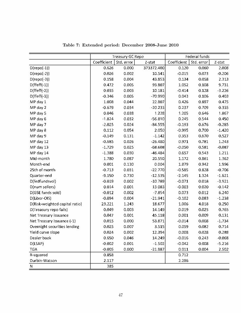
Table 7: Extended period: December 2008-June 2010C o e f f i c i e n t S t d . e r r o r Z - s t a t C o e f f i c i e n t S t d . e r r o r Z - s t a tD ( r e p o ( - 1 ) ) 0 . 6 2 6 0 . 0 0 0 3 7 3 3 7 2 . 4 0 0 0 . 1 2 0 0 . 0 6 0 2 . 0 0 8D ( r e p o ( - 2 ) ) 0 . 0 2 6 0 . 0 0 2 1 0 . 5 4 1 - 0 . 0 1 5 0 . 0 7 3 - 0 . 2 0 6D ( r e p o ( - 3 ) ) 0 . 1 5 8 0 . 0 0 4 4 3 . 8 5 3 0 . 1 3 4 0 . 0 5 8 2 . 3 1 3D ( f f e f f ( - 1 ) ) 0 . 4 7 2 0 . 0 0 5 9 3 . 8 0 7 1 . 0 5 2 0 . 1 0 8 9 . 7 3 1D ( f f e f f ( - 2 ) ) 0 . 0 3 5 0 . 0 0 3 1 0 . 1 8 1 - 0 . 4 1 4 0 . 1 2 8 - 3 . 2 2 6D ( f f e f f ( - 3 ) ) - 0 . 3 4 6 0 . 0 0 5 - 7 0 . 9 9 0 0 . 0 4 3 0 . 1 0 6 0 . 4 0 3M P d a y 1 1 . 0 0 8 0 . 0 4 4 2 2 . 8 0 7 0 . 4 2 6 0 . 8 9 7 0 . 4 7 5M P d a y 2 - 0 . 6 7 9 0 . 0 3 4 - 2 0 . 2 3 3 0 . 2 3 7 0 . 7 0 9 0 . 3 3 5M P d a y 5 0 . 0 4 6 0 . 0 3 8 1 . 2 2 8 1 . 2 0 5 0 . 6 4 6 1 . 8 6 7M P d a y 6 - 1 . 8 2 4 0 . 0 3 2 - 5 6 . 8 1 0 0 . 2 4 5 0 . 5 4 4 0 . 4 5 0M P d a y 7 - 2 . 0 2 5 0 . 0 2 4 - 8 4 . 5 5 5 - 0 . 1 9 3 0 . 6 7 6 - 0 . 2 8 5M P d a y 8 0 . 1 1 2 0 . 0 5 4 2 . 0 5 0 - 0 . 9 9 5 0 . 7 0 0 - 1 . 4 2 0M P d a y 9 - 0 . 1 4 9 0 . 1 3 1 - 1 . 1 4 2 0 . 3 5 3 0 . 6 7 0 0 . 5 2 7M P d a y 1 2 - 0 . 6 8 5 0 . 0 2 6 - 2 6 . 4 8 0 0 . 9 7 1 0 . 7 8 1 1 . 2 4 3M P d a y 1 3 - 1 . 7 2 9 0 . 0 2 5 - 6 8 . 6 0 8 - 0 . 0 5 0 0 . 5 8 1 - 0 . 0 8 7M P d a y 1 4 - 1 . 3 8 8 0 . 0 3 0 - 4 6 . 4 8 4 0 . 6 5 7 0 . 5 4 3 1 . 2 1 1M i d - m o n t h 1 . 7 8 0 0 . 0 8 7 2 0 . 5 5 0 1 . 1 7 2 0 . 8 6 1 1 . 3 6 2M o n t h - e n d 0 . 0 0 1 0 . 1 3 0 0 . 0 0 4 1 . 8 7 9 0 . 9 4 2 1 . 9 9 62 5 t h o f m o n t h - 0 . 7 1 3 0 . 0 3 1 - 2 2 . 7 7 0 - 0 . 5 8 5 0 . 8 2 8 - 0 . 7 0 6Q u a r t e r - e n d - 9 . 1 5 0 0 . 7 3 0 - 1 2 . 5 3 5 - 2 . 1 4 5 1 . 3 2 4 - 1 . 6 2 1D ( f e d f u n d s v o l ) - 0 . 0 1 9 0 . 0 0 2 - 1 0 . 7 8 9 - 0 . 0 7 1 0 . 0 1 8 - 3 . 9 2 1D ( n u m s e l l e r s ) 0 . 0 1 4 0 . 0 0 1 1 3 . 0 8 3 - 0 . 0 0 3 0 . 0 2 0 - 0 . 1 4 2D ( G S E f u n d s s o l d ) - 0 . 0 1 2 0 . 0 0 2 - 7 . 8 5 4 0 . 0 7 3 0 . 0 1 2 6 . 2 4 0D ( L i b o r - O I S ) - 0 . 0 9 4 0 . 0 0 4 - 2 1 . 9 4 1 - 0 . 1 0 2 0 . 0 8 3 - 1 . 2 3 8D ( R i s k - w e i g h t e d c a p i t a l r a t i o ) 2 3 . 2 2 1 1 . 2 4 3 1 8 . 6 7 7 1 . 0 0 6 4 . 0 1 8 0 . 2 5 0D ( T r e a s u r y r e p o f a i l s ) 0 . 0 4 9 0 . 0 0 3 1 4 . 1 4 9 0 . 0 1 9 0 . 0 2 5 0 . 7 6 5N e t T r e a s u r y i s s u a n c e 0 . 0 4 7 0 . 0 0 1 4 5 . 1 1 8 0 . 0 0 1 0 . 0 0 9 0 . 1 3 1N e t T r e a s u r y i s s u a n c e ( - 1 ) 0 . 0 1 5 0 . 0 0 0 5 3 . 8 7 1 - 0 . 0 1 4 0 . 0 0 8 - 1 . 7 3 4O v e r n i g h t s e c u r i t i e s l e n d i n g 0 . 0 2 5 0 . 0 0 7 3 . 5 1 5 0 . 0 5 9 0 . 0 8 2 0 . 7 1 4Y i e l d c u r v e s l o p e 0 . 0 2 4 0 . 0 0 2 1 2 . 3 9 4 0 . 0 0 8 0 . 0 2 8 0 . 2 8 8D e a l e r b o o k 0 . 6 5 0 0 . 0 4 6 1 4 . 2 4 9 - 0 . 0 1 6 0 . 2 4 3 - 0 . 0 6 8D ( L S A P ) - 0 . 0 0 2 0 . 0 0 1 - 1 . 5 0 2 - 0 . 0 4 2 0 . 0 0 8 - 5 . 2 1 6T G A - 0 . 0 0 5 0 . 0 0 0 - 2 1 . 8 8 7 0 . 0 1 1 0 . 0 0 4 2 . 5 0 2R - s q u a r e d 0 . 8 5 8 0 . 7 1 2D u r b i n - W a t s o n 2 . 1 1 7 2 . 2 8 6N 3 8 5

T r e a s u r y G C R e p o F e d e r a l f u n d s

47