AQA Level 2 Certificate in

Further Mathematics

The Need-To-Know Book for Further Maths Level 2 Everything you need to know for Further Maths Level 2

Examination Board: AQA

Page 1 of 27

Brief This document is intended as an aid for revision. Although it includes some examples and explanation, it is primarily not for learning content, but for becoming familiar with the requirements of the course as regards formulae and results. It cannot replace the use of a text book, and nothing produces competence and familiarity with mathematical techniques like practice. This document was produced as an addition to classroom teaching and textbook questions, to provide a summary of key points and, in particular, any formulae or results you are expected to know and use for this qualification. Note: The Further Maths Level 2 course is intended for those who have achieved, or are expecting to achieve, an A or A* grade in GCSE Mathematics. As such, a thorough knowledge of the GCSE course is required as a prerequisite to this course. Contents

Page Topic

2 Section 1 – Number

5 Section 2 – Algebra

14 Section 3 – Coordinate Geometry

17 Section 4 – Calculus

20 Section 5 – Matrix Transformations

23 Section 6 – Geometry

Page 2 of 27

Section 1 – Number Fractions

When adding or subtracting fractions, write over a common denominator, then add or subtract the numerators. Answers should be simplified where possible.

Note: If adding fractions in mixed number form, it is often easiest to add the whole number and fraction parts separately. Eg:

44

5+ 5

3

7= (4 + 5) + (

4

5+

3

7) = 9 + (

28

35+

15

35) = 9 + (

43

35) = 9 + (1

8

35) = 𝟏𝟎

𝟖

𝟑𝟓

When multiplying fractions, there is no need to find a common denominator. Simply multiply the numerators and multiply the denominators.

Note: If multiplying fractions in mixed number form, first write as improper fractions. Note: For large numbers it can help to identify common factors in the numerators and denominators and pre-cancel before multiplying together. Eg:

8

15×

9

16=

1

5×

3

2=

𝟑

𝟏𝟎

Here the 8 and 16 were both divided by 8, and the 9 and 15 were both divided by 3.

When dividing fractions, multiply by the reciprocal of the fraction you want to divide by.

Note: If dividing fractions in mixed number form, first write as improper fractions.

When finding a percentage of an amount, convert to a decimal and multiply.

Eg:

26% 𝑜𝑓 £400 = 0.26 × 400 = £𝟏𝟎𝟒

To increase or decrease by a percentage, multiply by the appropriate decimal.

Eg: Increase 50kg by 15%: 1.15 × 50 = 𝟓𝟕. 𝟓𝒌𝒈. Decrease 80cm by 8%: 0.92 × 80 = 𝟕𝟑. 𝟔𝒄𝒎.

Page 3 of 27

To reverse a percentage change, divide by the relevant decimal multiplier.

Eg: A coat is marked down 30% in a sale. If the sale price is £43.40, what was the original price?

£43.4 ÷ 0.7 = £𝟔𝟐

To apply compound interest for 𝑛 years, raise the decimal multiplier to the power 𝑛.

Eg: James borrows £2500 at an annual interest rate of 17%. How much will he owe after 8 years?

£2500 × 1.178 = £𝟖𝟕𝟕𝟖. 𝟔𝟑

To share an amount in a ratio, find the total number of parts, then scale up to the required total.

Eg: Julie and Kate work 8 hours and 14 hours respectively each week at a restaurant, and any tips received are shared in this ratio. One week they receive £55 in tips. How much does Kate receive?

8 ∶ 14 ⟺ 4 ∶ 7

Julie Kate Total 4 : 7 11

× 5 × 5 × 5 20 : 35 55

𝑲𝒂𝒕𝒆 𝒓𝒆𝒄𝒆𝒊𝒗𝒆𝒔 £𝟑𝟓

Ratios can be combined by making the parts equal. This can be done by forming equivalent ratios.

Eg: There is twice as much sugar as flour in a recipe, and 2 parts butter to 3 parts sugar. What is the ratio of sugar to flour to butter?

𝑆 ∶ 𝐹 = 2 ∶ 1 𝐵 ∶ 𝑆 = 2 ∶ 3

𝑆 ∶ 𝐹 = 6 ∶ 3 𝐵 ∶ 𝑆 = 4 ∶ 6

𝐹 ∶ 𝑆 = 3 ∶ 6 𝑆 ∶ 𝐵 = 6 ∶ 4

𝐹 ∶ 𝑆 ∶ 𝐵 = 3 ∶ 6 ∶ 4

𝑆 ∶ 𝐹 ∶ 𝐵 = 𝟔 ∶ 𝟑 ∶ 𝟒

Page 4 of 27

Surds

A surd is an irrational number involving a root. An irrational number is one that cannot be written as a fraction with whole numbers forming the numerator and denominator.

Eg: √5 is a surd. √16 = 4 so it is not a surd. Neither is √25

4 as √

25

4=

√25

√4=

5

2.

Multiplication or division within a root can be brought outside the root. In general:

√𝑎𝑏 = √𝑎 × √𝑏 𝑎𝑛𝑑 √𝑎

𝑏=

√𝑎

√𝑏

Note: Remember that addition does not work in the same way. For instance, √9 + 16 ≠ √9 + √16. Eg: A right-angled triangle has sides of 12𝑐𝑚 and 8𝑐𝑚. Find the possible lengths of the third side.

𝐵𝑦 𝑃𝑦𝑡ℎ𝑎𝑔𝑜𝑟𝑎𝑠′ 𝑡ℎ𝑒𝑜𝑟𝑒𝑚:

𝑂𝑝𝑡𝑖𝑜𝑛 1 (𝑚𝑖𝑠𝑠𝑖𝑛𝑔 𝑠𝑖𝑑𝑒 ℎ𝑦𝑝𝑜𝑡𝑒𝑛𝑢𝑠𝑒): √122 + 82 = √208 = √16√13 = 𝟒√𝟏𝟑

𝑂𝑝𝑡𝑖𝑜𝑛 2 (𝑚𝑖𝑠𝑠𝑖𝑛𝑔 𝑠𝑖𝑑𝑒 𝑛𝑜𝑡 ℎ𝑦𝑝𝑜𝑡𝑒𝑛𝑢𝑠𝑒): √122 − 82 = √80 = √16√5 = 𝟒√𝟓

If a fraction has a surd in the denominator, it is often useful to rewrite the fraction in such a way as to have only rational numbers in the denominator. This is called rationalising the denominator. This is done, in simple cases, by simply multiplying top and bottom by the surd in the denominator:

𝑎

√𝑏=

𝑎

√𝑏×

√𝑏

√𝑏=

𝑎√𝑏

𝑏

Eg: Simplify the following expression as far as possible: 5

√8− √18 +

√80

√5

5

√8− √18 +

√160

√5=

5√8

8− 3√2 +

4√10√5

5=

10√2

8− 3√2 +

4√2√5√5

5=

5√2

4− 3√2 + 4√2 =

𝟗√𝟐

𝟒

To rationalise the denominator of a more complex fraction, use the difference of two squares:

𝑎

𝑏 + √𝑐=

𝑎(𝑏 − √𝑐)

(𝑏 + √𝑐)(𝑏 − √𝑐)=

𝑎𝑏 − 𝑎√𝑐

𝑏2 − 𝑐

Eg:

6

3 − 2√5=

6(3 + 2√5)

(3 − 2√5)(3 + 2√5)=

18 + 12√5

9 − 20=

18 + 12√5

−11= −

𝟔(𝟑 + 𝟐√𝟓)

𝟏𝟏

Page 5 of 27

Section 2 – Algebra Expressions

To multiply out brackets, multiply every term within the bracket by the multiplier outside: 𝑎(𝑏 + 𝑐) = 𝑎𝑏 + 𝑎𝑐

Note: You will also need to be familiar with rules of indices when dealing with these questions. Eg: Expand the expression 3𝑥4𝑦(2𝑥𝑦 − 5𝑥3)

3𝑥4𝑦(2𝑥𝑦 − 5𝑥3) = 3𝑥4𝑦 × 2𝑥𝑦 − 3𝑥4𝑦 × 5𝑥3 = 𝟔𝒙𝟓𝒚𝟐 − 𝟏𝟓𝒙𝟕𝒚

When simplifying an algebraic expression where terms are added, you can collect like terms.

Eg: Simplify 3𝑥(2 − 5𝑥) − 7(𝑥 − 5)

3𝑥(2 − 5𝑥) − 7(𝑥 − 5) = 6𝑥 − 15𝑥2 − (7𝑥 − 35) = 6𝑥 − 15𝑥2 − 7𝑥 + 35 = 𝟑𝟓 − 𝒙 − 𝟏𝟓𝒙𝟐

To multiply brackets together, every term in each bracket must be multiplied: (𝑎 + 𝑏)(𝑐 + 𝑑) = 𝑎𝑐 + 𝑎𝑑 + 𝑏𝑐 + 𝑏𝑑

Note: To multiply out more than two brackets, it is usually easiest to take one pair at a time. Eg: Multiply out (3𝑥 − 1)(𝑥 + 4)(2 − 𝑥)

(3𝑥 − 1)(𝑥 + 4)(2 − 𝑥) = (3𝑥 − 1)(2𝑥 − 𝑥2 + 8 − 4𝑥) = (3𝑥 − 1)(8 − 2𝑥 − 𝑥2)

= 24𝑥 − 6𝑥2 − 3𝑥3 − 8 + 2𝑥 + 𝑥2 = −𝟖 + 𝟐𝟔𝒙 − 𝟓𝒙𝟐 − 𝟑𝒙𝟑

To factorise an expression fully, it is necessary to find terms (numbers, letters or a combination) which are factors of every term in the bracket.

Eg: Fully factorise 28𝑥3𝑦2 − 12𝑥5𝑦7

28𝑥3𝑦7 − 12𝑥5𝑦2 = 𝟒𝒙𝟑𝒚𝟐(𝟕𝒚𝟓 − 𝟑𝒙𝟐)

Page 6 of 27

Quadratics

A quadratic function can be written in the form 𝑦 = 𝑎𝑥2 + 𝑏𝑥 + 𝑐, and the shape of the graph produced is known as a parabola. It is symmetrical, and resembles either ∪ (for 𝑎 > 0) or ∩ (for 𝑎 <0). If it crosses the 𝑥-axis, the equation 𝑎𝑥2 + 𝑏𝑥 + 𝑐 = 0 has two distinct solutions. If it only touches at one point this will be at its maximum or minimum and the equation will have one (repeated) solution. If the graph doesn’t touch the 𝑥-axis at all, the equation will have no real solutions.

To factorise a quadratic, it is often necessary to find more than a single term, forming two brackets.

Note: If the quadratic has only an 𝑥2 and an 𝑥 term, 𝑥 will be a factor, so factorising becomes simpler.

To factorise expressions with a single 𝒙𝟐 term, write out two brackets with 𝑥 at the start of each. To determine the numbers to go alongside these, find two numbers that multiply to make the constant term but add to make the 𝑥 coefficient.

Eg: Solve 𝑥2 − 5𝑥 + 4 = 0 𝑥2 − 5𝑥 + 4 = (𝑥 … )(𝑥 … ) and since −1 and −4 multiply to make 4 but add to make −5:

𝑥2 − 5𝑥 + 4 = 0 ⟹ (𝑥 − 1)(𝑥 − 4) = 0 ⟹ 𝒙 = 𝟏 𝒐𝒓 𝒙 = 𝟒

To factorise expressions with a number in front of 𝒙𝟐, before splitting into brackets, find two numbers that multiply to make the product of the 𝑥2 coefficient and the constant, but add to make the 𝑥 coefficient. Then split the 𝑥 term into these two parts, factorise the first two terms of the expression separately, then the last two terms, and finally factorise the whole thing.

Eg: Solve: 2𝑥2 + 𝑥 − 3 = 0 Two numbers which multiply to make 2 × −3 = −6 and add to make 1: 3 and −2, so:

2𝑥2 + 𝑥 − 3 = 2𝑥2 + 3𝑥 − 2𝑥 − 3 = 𝑥(2𝑥 + 3) − 1(2𝑥 + 3) = (2𝑥 + 3)(𝑥 − 1)

⟹ (2𝑥 + 3)(𝑥 − 1) = 0 ⟹ 𝒙 = −𝟑

𝟐 𝒐𝒓 𝒙 = 𝟏

Page 7 of 27

Another way to solve a quadratic is completing the square. This will work for any quadratic, but can take longer than factorising for simpler equations. Note also that completing the square is a technique that can be used to determine a maximum or minimum point on a quadratic graph without solving the equation. The aim is to write the quadratic expression in the form p(x + q)2 + r, as shown below.

Eg: Solve 𝑥2 + 6𝑥 + 10 = 0 by completing the square.

Step 1: Halve the 𝑥 coefficient to find the number to go with 𝑥 in the squared bracket:

(𝑥 + 3)2 We know that if we multiply this out we would get 𝑥2 + 6𝑥 + 9

Step 2: Subtract the square of this number from the squared bracket:

(𝑥 + 3)2 − 9 By subtracting the 9 we make an expression equal to 𝑥2 + 6𝑥

Step 3: Add the constant from the original expression, and simplify:

(𝑥 + 3)2 − 9 + 10 = (𝒙 + 𝟑)𝟐 + 𝟏 This is equal to 𝑥2 + 6𝑥 + 10, but written as a completed square

Step 4: We can then solve the equation by rearranging (notice that now 𝑥 occurs just once):

𝑥2 + 6𝑥 − 5 = (𝑥 + 3)2 − 9 + 1 = (𝑥 + 3)2 − 8 ⟹ (𝑥 + 3)2 − 8 = 0

⟹ (𝑥 + 3)2 = 8 ⟹ 𝑥 + 3 = ±√8 = ±2√2

⟹ 𝒙 = −𝟑 ± 𝟐√𝟐

The quadratic formula is the result of completing the square with the general form of a quadratic, 𝑎𝑥2 + 𝑏𝑥 + 𝑐 = 0. By dividing by 𝑎, completing the square and making 𝑥 the subject, we get:

𝑥 =−𝑏 ± √𝑏2 − 4𝑎𝑐

2𝑎

Note: Some quadratic equations have no solutions, some have exactly one, and some have two. By considering the value of 𝑏2 − 4𝑎𝑐 we can discriminate between these three cases. If 𝑏2 − 4𝑎𝑐 is positive, there are two distinct solutions, if 0, only one (a ‘repeated root’), and if negative, no real solutions. Formulae

To change the subject of a formula, first isolate the term required, then reverse the operations applied to it.

Note: If the term appears twice, it is often necessary to collect them and factorise the expression. Eg: Make 𝑥 the subject of the formula:

5𝑦 − 𝑥 =2𝑥 + 3

7𝑞2 ⟹ 7𝑞2(5𝑦 − 𝑥) = 2𝑥 + 3 ⟹ 35𝑞2𝑦 − 7𝑞2𝑥 = 2𝑥 + 3

⟹ 35𝑞2𝑦 − 3 = 2𝑥 + 7𝑞2𝑥 ⟹ 35𝑞2𝑦 − 3 = 𝑥(2 + 7𝑞2) ⟹ 35𝑞2𝑦 − 3

2 + 7𝑞2= 𝑥

Page 8 of 27

Rational expressions

To simplify, add or subtract rational expressions, simply apply the rules of fractions. You can cancel terms if they are factors of both the numerator and denominator (that is, divide top and bottom by the same thing), and to add or subtract fractions, write with a common denominator then combine the numerators by adding or subtracting. To divide by a fraction, multiply by its reciprocal.

Eg: Simplify 𝑥2−100

𝑥2+8𝑥−20

𝑥2 − 100

𝑥2 + 8𝑥 − 20=

(𝑥 + 10)(𝑥 − 10)

(𝑥 + 10)(𝑥 − 2)=

𝒙 − 𝟏𝟎

𝒙 − 𝟐

Eg: Simplify 𝑥+4

2𝑥−

𝑥−8

𝑥2−4𝑥

𝑥 + 4

2𝑥−

𝑥 − 8

𝑥2 − 4𝑥=

𝑥 + 4

2𝑥−

𝑥 − 8

𝑥(𝑥 − 4)=

(𝑥 + 4)(𝑥 − 4)

2𝑥(𝑥 − 4)−

2(𝑥 − 8)

2𝑥(𝑥 − 4)

=(𝑥 + 4)(𝑥 − 4) − 2(𝑥 − 8)

2𝑥(𝑥 − 3)=

𝑥2 − 16 − 2𝑥 + 16

2𝑥(𝑥 − 3)

=𝑥2 − 2𝑥

2𝑥(𝑥 − 3)=

𝑥(𝑥 − 2)

2𝑥(𝑥 − 3)=

𝒙 − 𝟐

𝟐(𝒙 − 𝟑)

Functions

A function is a mapping which can be either one-to-one or many-to-one.

Eg: 𝑓(𝑥) = 3𝑥 − 4 is a one-to-one function, 𝑓(𝑥) = 𝑥2 + 5 is a many-to-one function.

The domain of a function is the set of input values it can take. The range of a function is the set of output values it can generate.

Eg: 𝑓(𝑥) =5

𝑥2 has the domain 𝑥 ≠ 0 and the range 𝑓(𝑥) > 0.

A function is fully defined by both a rule and a domain.

Eg: 𝑓(𝑥) =2𝑥

(𝑥−3) 𝑓𝑜𝑟 𝑥 ≠ 3.

Factor theorem

The factor theorem: (𝑥 − 𝑎) 𝑖𝑠 𝑎 𝑓𝑎𝑐𝑡𝑜𝑟 𝑜𝑓 𝑝𝑜𝑙𝑦𝑛𝑜𝑚𝑖𝑎𝑙 𝑃(𝑥) ⟺ 𝑃(𝑎) = 0 (𝑡ℎ𝑎𝑡 𝑖𝑠, 𝑎 𝑖𝑠 𝑎 𝑟𝑜𝑜𝑡)

Note: This means that if we know a factor of a polynomial, we can find the corresponding root (a root is defined as the solution to 𝑓(𝑥) = 0; that is, the 𝑥 coordinates of points where the graph 𝑦 = 𝑓(𝑥) crosses the 𝑦-axis). The factor theorem works both ways, so if we know a root already, we can determine the corresponding factor.

Page 9 of 27

To factorise a cubic, first find a root by trial and error, then use the factor theorem to generate a linear factor. Finally, use inspection to find the remaining (quadratic) factor, and factorise this, where possible.

Eg: Factorise fully 2𝑥3 + 3𝑥2 − 16𝑥 + 15

𝑃(𝑥) = 2𝑥3 − 𝑥2 − 16𝑥 + 15

𝑃(0) = 15 ⟹ 0 𝑖𝑠 𝑛𝑜𝑡 𝑎 𝑟𝑜𝑜𝑡 𝑃(1) = 0 ⟹ 1 𝑖𝑠 𝑎 𝑟𝑜𝑜𝑡

𝐵𝑦 𝑡ℎ𝑒 𝑓𝑎𝑐𝑡𝑜𝑟 𝑡ℎ𝑒𝑜𝑟𝑒𝑚: 𝑃(1) = 0 ⟹ (𝑥 − 1) 𝑖𝑠 𝑎 𝑓𝑎𝑐𝑡𝑜𝑟

2𝑥3 − 𝑥2 − 16𝑥 + 15 = (𝑥 − 1)(… ) By inspection, we need 2𝑥2 in the second bracket to give the 2𝑥3 term in the cubic. We also need −15 in the second bracket to give the 15 term in the cubic.

𝑃(𝑥) = (𝑥 − 1)(2𝑥2 + ⋯ − 15) To get the 𝑥2 term we need to examine the 𝑥 terms from each, as well as the combination of the 𝑥2 and constant terms. Since we already have −1 × 2𝑥2 giving −2𝑥2, we need 𝑥2 to give the result – 𝑥2. This must be achieved by 𝑥 multiplied by the second bracket’s 𝑥 term which therefore must be simply 𝑥.

𝑃(𝑥) = (𝑥 − 1)(2𝑥2 + 𝑥 − 15) Finally, factorise the quadratic if possible:

𝑃(𝑥) = (𝑥 − 1)(2𝑥 − 5)(𝑥 + 3) Sketching curves

When sketching a quadratic, include: The correct shape: A positive quadratic (one with a positive 𝑥2 coefficient) will have a single turning point – a minimum – and a negative quadratic will have a maximum point. The graph will be symmetrical about its vertex (the max/min point), and should be a smooth curve with no sharp turns which gets steeper as it increases but never vertical. The 𝒚-intercept: The point at which the curve crosses the 𝑦-axis. There will always be one, and only one, for a quadratic, and it is easy to identify because the curve crosses the 𝑦-axis when 𝑥 = 0. Substituting 𝑥 = 0 into 𝑦 = 𝑎𝑥2 + 𝑏𝑥 + 𝑐 gives 𝑦 = 𝑐, so the intercept is (0, 𝑐). Any 𝒙-axis crossing points: These are points where the curve 𝑦 = 𝑎𝑥2 + 𝑏𝑥 + 𝑐 crosses the line 𝑦 =0, so they are solutions to 𝑎𝑥2 + 𝑏𝑥 + 𝑐 = 0 and can be found – if any exist – by either factorising, completing the square or applying the quadratic formula. There may be 0, 1 or 2 roots. [Sometimes required] The position of the vertex: By completing the square, it is possible to determine the coordinates of the maximum or minimum point. This allows a more precise sketch.

Page 10 of 27

When sketching a cubic, include: The correct shape: A positive cubic decreases without limit as 𝑥 decreases, and increases without limit as 𝑥 increases (so it tends to go from bottom left to top right). A negative does the opposite. Either can have a point of inflection in the middle (a ‘wiggle’), like 𝑦 = 𝑥3, or a maximum point and a minimum point. The 𝒚-intercept: Like with the quadratic, since this is simply the value of the cubic expression when 𝑥 = 0, it is just the constant term. Any 𝒙-axis crossing points: These are not always straightforward to find, and a cubic may have one, two (in this case one is also a maximum or a minimum) or three. Use factor theorem to determine the roots. [Sometimes required] The position of any stationary points: If there are stationary points (some cubics have no points where the gradient is zero, some have one, some two), these can be found

using differentiation and solving 𝑑𝑦

𝑑𝑥= 0. Their nature (maximim, minimum or point of inflection)

can be determined by considering the height ( 𝑦 ) or gradient ( 𝑑𝑦

𝑑𝑥 ) on either side.

Simultaneous equations

One method for solving simultaneous linear equations is the elimination method. Coefficients of one of the variables are made equal and then the equations are effectively added or subtracted from one another to eliminate this variable.

Eg: (1) 5𝑥 − 2𝑦 = 6 (2) 2𝑥 + 4𝑦 = 9 (1)×2 10𝑥 − 4𝑦 = 12

(2)+(1’) 12𝑥 = 21 ⟹ 𝑥 =21

12=

7

4= 1.75

Sub into (2) 2 (7

4) + 4𝑦 = 9 ⟹ 4𝑦 = 9 −

7

2=

11

2 ⟹ 𝑦 =

11

8= 1.375

More generally, a wider range of simultaneous equations can be solved using substitution.

Eg: (1) 𝑦 − 1 = 2𝑥 (2) 𝑦2 − 3𝑥2 = 6 Rearrange (1) 𝑦 = 2𝑥 − 1 Sub into (2) (2𝑥 − 1)2 − 3𝑥2 = 6 Rearrange (2’) 𝑥2 − 4𝑥 − 5 = 0 Solve (2’) (𝑥 + 1)(𝑥 − 5) = 0 ⟹ 𝑥 = −1 𝑜𝑟 𝑥 = 5 Sub into (1’) 𝑦 = 2(−1) − 1 = −3 𝑜𝑟 𝑦 = 2(5) − 1 = 9 Write out solutions 𝑥 = −1 𝑦 = −3 𝑜𝑟 𝑥 = 5 𝑦 = 9 Note: Take care to pair up the correct values of 𝑥 and 𝑦 – they represent the coordinates of the crossing points for the two equations.

Page 11 of 27

Inequalities

When solving a linear inequality, if you multiply or divide by a negative, you reverse the sign.

Note: The reason for this is clear when you consider 3 < 5. By subtracting 8 from each side we get −5 < −3, which is of course perfectly correct. But notice that this is equivalent to −3 > −5 which not only has different signs to the original statement but also has the inequality sign reversed.

To solve a quadratic inequality, it is necessary first to find the critical values (that is, the solutions to the related equation), then use a sketch to interpret these values as solution regions.

Eg: Solve 𝑥2 − 5𝑥 + 6 ≥ 0

Finding critical values: 𝑥2 − 5𝑥 + 6 = 0

⟹ (𝑥 − 2)(𝑥 − 3) = 0 ⟹ 𝑥 = 2 𝑎𝑛𝑑 𝑥 = 3 Interpreting the sketch:

𝑥 ≤ 2 𝑜𝑟 𝑥 ≥ 3

Sketching the curve:

Indices

The multiplication rule: 𝑎𝑚 × 𝑎𝑛 = 𝑎𝑚+𝑛

The division rule: 𝑎𝑚 ÷ 𝑎𝑛 = 𝑎𝑚−𝑛

The power rule: (𝑎𝑚)𝑛 = 𝑎𝑚𝑛

The negative index rule:

𝑎−𝑛 =1

𝑎𝑛

The zero index result: 𝑎0 = 1

The root rule:

𝑎1𝑛 = √𝑎

𝑛 𝑎𝑛𝑑, 𝑚𝑜𝑟𝑒 𝑔𝑒𝑛𝑒𝑟𝑎𝑙𝑙𝑦: 𝑎

𝑚𝑛 = √𝑎𝑚𝑛

= ( √𝑎𝑛

)𝑚

Page 12 of 27

Eg:

Simplify: √𝑥2𝑦34

𝑥𝑎−3

√𝑥2𝑦34

𝑥3= 𝑥

24𝑦

34𝑥−3 = 𝑥

12

−3𝑦34 = 𝒙−

𝟓𝟐𝒚

𝟑𝟒

Eg 2:

Solve: 33𝑥

27=

1

92𝑥+1

33𝑥

27=

1

92𝑥+1 ⟹

33𝑥

33= 9−2𝑥−1

⟹ 33𝑥−3 = (32)−2𝑥−1 ⟹ 33𝑥−3 = 3−4𝑥−2

⟹ 3𝑥 − 3 = −4𝑥 − 2 ⟹ 7𝑥 = 1 ⟹ 𝑥 =1

7

Algebraic proof

To prove a result, it is necessary to formulate your assumptions and define your variables. This is usually in the form of an algebraic statement such as an equation. Each line of your proof should then be the next line of a reasoned argument, with each statement being a necessary consequence of the previous one, finishing with a conclusion.

Eg: Prove that the difference between two consecutive cube numbers is not a multiple of 3. The difference between two consecutive cube numbers can be written as (𝑛 + 1)3 − 𝑛3

(𝑛 + 1)3 − 𝑛3 = 𝑛3 + 3𝑛2 + 3𝑛 + 1 − 𝑛3 = 3𝑛2 + 3𝑛 + 1 = 3𝑛(𝑛 + 1) + 1 Since 3𝑛(𝑛 + 1) has 3 as a factor, 3𝑛(𝑛 + 1) is necessarily a mutliple of 3. Therefore 3𝑛(𝑛 + 1) + 1 is not a multiple of 3. Sequences

To find the 𝑛𝑡ℎ term of a linear sequence, identify the common difference (the difference between any consecutive terms), and compare the sequence to the related multiplication table. Add or subtract the required value to transform this sequence into yours.

Eg: Prove that 340 is not in the linear sequence 6, 10, 14, 18, ….

𝑇(𝑛) = 4𝑛 ⟹ 4, 8, 12, … ⟹ 𝑇ℎ𝑖𝑠 𝑠𝑒𝑞𝑢𝑒𝑛𝑐𝑒 𝑚𝑢𝑠𝑡 𝑏𝑒 𝑇(𝑛) = 4𝑛 + 2

4𝑛 + 2 = 340 ⟹ 𝑛 =338

4= 84.5. 𝑁𝑜𝑡 𝑎 𝑤ℎ𝑜𝑙𝑒 𝑛𝑢𝑚𝑏𝑒𝑟 ⟹ 340 𝑛𝑜𝑡 𝑖𝑛 𝑠𝑒𝑞𝑢𝑒𝑛𝑐𝑒

Page 13 of 27

To find the 𝑛𝑡ℎ term of a quadratic sequence, find the sequence of differences, then the sequence of second differences. Halve the second difference to find the 𝑛2 coefficient. Find the difference between this simple quadratic sequence and your original sequence. Find the 𝑛𝑡ℎ term of this (linear) sequence and add it to the 𝑛2 part.

Eg: Find the 𝑛𝑡ℎ term rule of the quadratic sequence 12, 32, 62, 102, …. Sequence of differences: 20, 30, 40, … Sequence of second differences: 10, 10, 10, … Quadratic part: 𝑇(𝑛) = 5𝑛2 ⟹ 5, 20, 45, 80, … Difference: 7, 12, 17, 22, … ⟹ 𝑇(𝑛) = 5𝑛 + 2 Complete sequence: 𝑻(𝒏) = 𝟓𝒏𝟐 + 𝟓𝒏 + 𝟐

Some sequences tend towards a limit (that is, sucessive terms get increasingly close to, but never surpass, a particular value). Depending on the 𝑛𝑡ℎ term rule for these sequences, the limit can be

found through algebraic manipulation, using the fact that 1

𝑛 tends to 0 as 𝑛 ‘tends to ∞’ (aka

‘increases without limit’).

Eg:

Find the limit of the sequence defined by 𝑇(𝑛) =8𝑛−4

4𝑛+20

Step 1: Divide through (top and bottom of the fraction) by 𝑛:

𝑇(𝑛) =8 −

4𝑛

4 +20𝑛

Step 2: Use the fact that 1

𝑛→ 0 as 𝑛 → ∞:

8 −4𝑛

4 +20𝑛

→8 − 0

4 + 0= 2 𝑎𝑠 𝑛 → ∞ 𝑡ℎ𝑒𝑟𝑒𝑓𝑜𝑟𝑒 𝒕𝒉𝒆 𝒍𝒊𝒎𝒊𝒕 𝒐𝒇 𝒕𝒉𝒆 𝒔𝒆𝒒𝒖𝒆𝒏𝒄𝒆 𝒊𝒔 𝟐

Page 14 of 27

Section 3 – Coordinate Geometry Straight lines

The distance between two points can be calculated by constructing a right-angled triangle between the coordinates and applying Pythagoras’ Theorem:

𝐷𝑖𝑠𝑡𝑎𝑛𝑐𝑒 𝑏𝑒𝑡𝑤𝑒𝑒𝑛 (𝑥1, 𝑦1) 𝑎𝑛𝑑 (𝑥2, 𝑦2): √(𝑥2 − 𝑥1)2 + (𝑦2 − 𝑦1)2

The midpoint of the line between the points (𝑥1, 𝑦1) and (𝑥2, 𝑦2) is given by:

(𝑥1 + 𝑥2

2,𝑦1 + 𝑦2

2)

Note: This is simply the average of the 𝑥 coordinates and the average of the 𝑦 coordinates.

If you are required to find a point which is a given proportion of the way between two points, it can be helpful to think in terms of adding a certain fraction of the journey to the starting point.

Eg: The point 1

3 of the way between (𝑥1, 𝑦1) and (𝑥2, 𝑦2) is: (𝑥1 +

1

3(𝑥2 − 𝑥1), 𝑦1 +

1

3(𝑦2 − 𝑦1))

Note: This can be simplified, in this case, to (2

3𝑥1 +

1

3𝑥2,

2

3𝑦1 +

1

3𝑦2), or, alternatively, the midpoint

formula can be rewritten to say: (𝑥1 +1

2(𝑥2 − 𝑥1), 𝑦1 +

1

2(𝑦2 − 𝑦1)).

The gradient of the line between the points (𝑥1, 𝑦1) and (𝑥2, 𝑦2) is given by:

𝑚 =𝑦2 − 𝑦1

𝑥2 − 𝑥1

Note: This is often described as ‘𝑦 step over 𝑥 step’, or ‘rise over run’.

Lines with gradients 𝑚1 and 𝑚2 are parallel if 𝑚1 = 𝑚2. They are perpendicular if 𝑚1𝑚2 = −1.

Note: The concepts behind the above results are more important (and more easily memorable) than the formulae used to describe them mathematically. The result below is the only one where memorising the formula gives a definite advantage to quickly solving problems, especially since simplification into a specific form is not always required.

Given the gradient, 𝑚, and a single point, (𝑥1, 𝑦1), the equation of a line can be generated using:

𝑦 − 𝑦1 = 𝑚(𝑥 − 𝑥1)

Page 15 of 27

Given two points, the equation of a line can be generated using:

𝑦 − 𝑦1

𝑦2 − 𝑦1=

𝑥 − 𝑥1

𝑥2 − 𝑥1

Note: The above result is simply a combination of the definition of gradient and the gradient & point formula above. As such it is not necessary to memorise this form if you are already confident with finding the gradient between two points and can recall 𝑦 − 𝑦1 = 𝑚(𝑥 − 𝑥1).

The crossing point of two lines directly corresponds with the values of 𝒙 and 𝒚 which satisfy both equations. This can be found either by reading off the graph, or – more precisely – by solving the equations simultaneously.

Circles

The equation of a circle with centre (0,0) and radius 𝑟 is given by:

𝑥2 + 𝑦2 = 𝑟2

Note: This can be understood by considering any point on the circle and constructing a right-angled triangle, with the line from the origin to the point as the hypotenuse. By Pythagoras’ Theorem, the square of the radius must be equal to the sum of the squares of the 𝑥 and 𝑦 coordinates.

The general equation of a circle with centre (𝑎, 𝑏) and radius 𝑟 is given by:

(𝑥 − 𝑎)2 + (𝑦 − 𝑏)2 = 𝑟2

Note: This is simply a translation from the original circle – centre (0,0) – by vector [𝑎𝑏

].

Eg: The circle (𝑥 − 3)2 + 𝑦2 = 25: Note: The most common mistakes to watch out for when interpreting a circle equation are getting the signs wrong for the centre coordinates or forgetting to square root the number on the right to get the radius.

Page 16 of 27

To sketch a circle: Step 1: Find the radius and centre from the equation. Step 2: Mark the centre. Step 3: Use the radius to mark on the four points directly above, below and to either side. Step 4: Draw the circle through these four points, indicating where the circle crosses the axes, if applicable.

Note: you may also have to rely on other circle facts such as how to calculate the circumference or area, or the circle theorems (see section 6 for details).

To find the equation of a circle given the end points of the diameter, calculate the midpoint and the distance between the points. This will give you the centre and the diameter. Halve the diameter to get the radius, then put into the form (𝑥 − 𝑎)2 + (𝑦 − 𝑏)2 = 𝑟2.

Like any other curve, the crossing points of a line and a circle can be found by solving simultaneously (using the substitution method).

A tangent to the circle at a particular point is a line which touches the circle only at that point. It is always perpendicular to the radius.

A normal to the circle at a particular point is a line passing through a circle which is perpendicular to the tangent at that point.

Note: The normal line at any point on a circle will pass through the centre, since it is perpendicular to the tangent which is perpendicular to the radius.

To find the equation of a tangent or normal at a particular point: Step 1: Find the centre of the circle. Step 2: Calculate the gradient of the line segment from the centre to your point. Step 3i: For a normal, use this gradient and your point in the formula 𝑦 − 𝑦1 = 𝑚(𝑥 − 𝑥1).

Step 3ii: For a tangent, first find the tangent gradient by using 𝑚1 = −1

𝑚2, then use the formula.

Note: You may need to complete the square to convert a circle equation into the preferred form first. Eg: Find the equation of the tangent to the circle 𝑥2 + 2𝑥 + 𝑦2 − 6𝑦 = 25 at the point (2,7).

𝑥2 + 2𝑥 + 𝑦2 − 6𝑦 = 25 ⟹ (𝑥 + 1)2 − 1 + (𝑦 − 3)2 − 9 = 25 ⟹ (𝑥 + 1)2 + (𝑦 − 3)2 = 35

𝐶𝑒𝑛𝑡𝑟𝑒: (−1,3) ⟹ 𝐺𝑟𝑎𝑑 𝑜𝑓 𝑟𝑎𝑑𝑖𝑢𝑠 𝑙𝑖𝑛𝑒: 7 − 3

2 − (−1)=

4

3 ⟹ 𝐺𝑟𝑎𝑑 𝑜𝑓 𝑡𝑎𝑛𝑔𝑒𝑛𝑡: −

1

43

= −3

4

𝐸𝑞𝑢𝑎𝑡𝑖𝑜𝑛 𝑜𝑓 𝑡𝑎𝑛𝑔𝑒𝑛𝑡: 𝑦 − 7 = −3

4(𝑥 − 2) ⟹ 𝑦 = −

3

4𝑥 +

17

2

Page 17 of 27

Section 4 – Calculus Differentiation is a method for finding the gradient of a curve at any given point. It can be thought of as the rate of change of 𝑦 with respect to 𝑥.

For a small change in 𝑥 and a corresponding small change in 𝑦, the gradient of a chord can be written as:

𝛿𝑦

𝛿𝑥

Note: Here, ‘chord’ refers to a straight line segment drawn between two nearby points on a curve. Gradient

We define the gradient of a curve at a particular point as the gradient of the tangent to the curve at that point.

Note: As the end-points get closer together, the gradient of the chord approaches the gradient of the tangent at each point (ie, the gradient of the curve). This is the basis for differentiation – the limit to which the gradients of the ever-decreasing chords tends is the gradient of the curve at that point.

The limit of 𝛿𝑦

𝛿𝑥 as 𝛿𝑦, 𝛿𝑥 → 0 is written as

𝑑𝑦

𝑑𝑥 and is known as the differential of 𝑦 with respect to 𝑥.

Note: The proof of this idea involves the concept of shrinking a small quantity until it is essentially of zero size. This is effectively finding the gradient of a chord connecting a point to itself. While this idea is worth being aware of, it is not necessary to memorise a proof of it.

𝑦 = 𝑥𝑛 ⟹ 𝑑𝑦

𝑑𝑥= 𝑛𝑥𝑛−1

Note: This can be thought of as “bring the power down in front, then reduce the power by one”. Note: If there is a number multiplied by the 𝑥𝑛 term, this is not affected by differentiating. Eg:

𝑦 = 5𝑥4 ⟹ 𝑑𝑦

𝑑𝑥= 20𝑥3

𝑦 = 𝑓(𝑥) ± 𝑔(𝑥) ⟹ 𝑑𝑦

𝑑𝑥= 𝑓′(𝑥) ± 𝑔′(𝑥)

Eg: The differential of 2𝑥4 − 8𝑥2 + 4 is 8𝑥3 − 16𝑥 (note that any constants differentiate to 0).

Note: 𝑓′(𝑥) is sometimes used to denote the derivative of 𝑓(𝑥). It is equivalent to 𝑑(𝑓(𝑥))

𝑑𝑥.

Page 18 of 27

To find the gradient of a curve at a particular point, calculate 𝑑𝑦

𝑑𝑥 and substitute in the 𝑥 coordinate.

Eg: Find the gradient of the curve 𝑦 = (2𝑥 + 3)(𝑥2 − 5) at the point (2, −7). Multiply out:

𝑦 = (2𝑥 + 3)(𝑥2 − 5) = 2𝑥3 + 3𝑥2 − 10𝑥 − 15 Differentiate:

𝑑𝑦

𝑑𝑥= 6𝑥2 + 6𝑥 − 10

Substitute in 𝑥 = 2:

𝐴𝑡 𝑥 = 2 𝑑𝑦

𝑑𝑥= 6(22) + 6(2) − 10 = 26 ⟹ 𝐺𝑟𝑎𝑑𝑖𝑒𝑛𝑡 = 26

To find a point on a curve with a given gradient, differentiate then set your expression equal to the gradient and solve for 𝑥. Finally, substitute into the original equation for a corresponding value for 𝑦.

Eg: Find any points on the curve 𝑦 = 𝑥3 − 3𝑥 where the gradient is 45. Differentiate:

𝑑𝑦

𝑑𝑥= 3𝑥2 − 3

Rewrite using 𝑑𝑦

𝑑𝑥= 45:

45 = 3𝑥2 − 3 ⟹ 𝑥2 − 1 = 15 ⟹ 𝑥2 = 16 ⟹ 𝑥 = ±4 Substitute back into the original equation:

𝐹𝑜𝑟 𝑥 = 4: 𝑦 = 43 − 3(4) = 52 ⟹ (4,52)

𝐹𝑜𝑟 𝑥 = −4: 𝑦 = (−4)3 − 3(−4) = −52 ⟹ (−4, −52)

Given the gradient of a curve at a particular point, we can find the equation of the tangent using 𝑦 −𝑦1 = 𝑚(𝑥 − 𝑥1) where (𝑥1, 𝑦1) is the point on the curve and 𝑚 is the gradient. Eg: Find the equation of the tangent to the curve 𝑦 = 5𝑥3 − 6 at the point (1, −1).

𝑑𝑦

𝑑𝑥= 15𝑥2 𝐴𝑡 𝑥 = 1: 𝑚 = 15(12) = 15 ⟹ 𝑢𝑠𝑖𝑛𝑔 𝑦 − 𝑦1 = 𝑚(𝑥 − 𝑥1)

𝑦 − (−1) = 15(𝑥 − 1) ⟹ 𝑦 = 15𝑥 − 16

Page 19 of 27

Stationary points

Recall that 𝑑𝑦

𝑑𝑥 means the rate of change of 𝑦 with respect to 𝑥.

𝑑𝑦

𝑑𝑥> 0 ⟹ 𝑦 𝑖𝑛𝑐𝑟𝑒𝑎𝑠𝑒𝑠 𝑎𝑠 𝑥 𝑖𝑛𝑐𝑟𝑒𝑎𝑠𝑒𝑠

𝑑𝑦

𝑑𝑥< 0 ⟹ 𝑦 𝑑𝑒𝑐𝑟𝑒𝑎𝑠𝑒𝑠 𝑎𝑠 𝑥 𝑖𝑛𝑐𝑟𝑒𝑎𝑠𝑒𝑠

Note: Often the rate of change will be with respect to time.

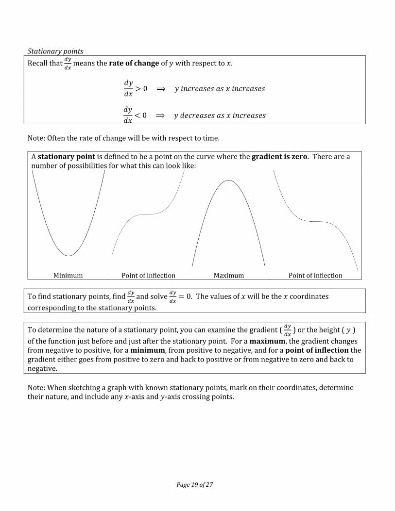
A stationary point is defined to be a point on the curve where the gradient is zero. There are a number of possibilities for what this can look like:

Minimum Point of inflection Maximum Point of inflection

To find stationary points, find 𝑑𝑦

𝑑𝑥 and solve

𝑑𝑦

𝑑𝑥= 0. The values of 𝑥 will be the 𝑥 coordinates

corresponding to the stationary points.

To determine the nature of a stationary point, you can examine the gradient ( 𝑑𝑦

𝑑𝑥 ) or the height ( 𝑦 )

of the function just before and just after the stationary point. For a maximum, the gradient changes from negative to positive, for a minimum, from positive to negative, and for a point of inflection the gradient either goes from positive to zero and back to positive or from negative to zero and back to negative.

Note: When sketching a graph with known stationary points, mark on their coordinates, determine their nature, and include any 𝑥-axis and 𝑦-axis crossing points.

Page 20 of 27

Section 5 – Matrix Transformations Terminology

A matrix is a rectangular array of numbers. Each entry in the matrix is called an element.

A matrix with m rows and n columns is an 𝑚 × 𝑛 matrix. This is called the order of the matrix.

We can add or subtract matrices provided they have the same order.

To add or subtract matrices, all that is required is that we add or subtract corresponding elements from each matrix.

Eg:

[3 2 5

−1 0 2] − [

6 1 10 −4 10

] = [−3 1 4−1 4 −8

]

Multiplication

To multiply a matrix by a constant, simply multiply each element of the matrix by the constant.

Note: This is comparable to finding the scalar multiple of a vector – in fact, that process is just a specific example of multiplying a matrix by a constant. Eg:

5 [1 23 1

] = [5 10

15 5]

We can multiply two matrices A and B only if the number of columns of A equals the number of rows of B.

Note: This does not mean the matrices have to be of equal order, but due to the method used for multiplying matrices, they must fulfil this requirement. You will only be required to multiply a 2 𝑏𝑦 2 matrix by either a 2 𝑏𝑦 1 vector or another 2 𝑏𝑦 2 matrix.

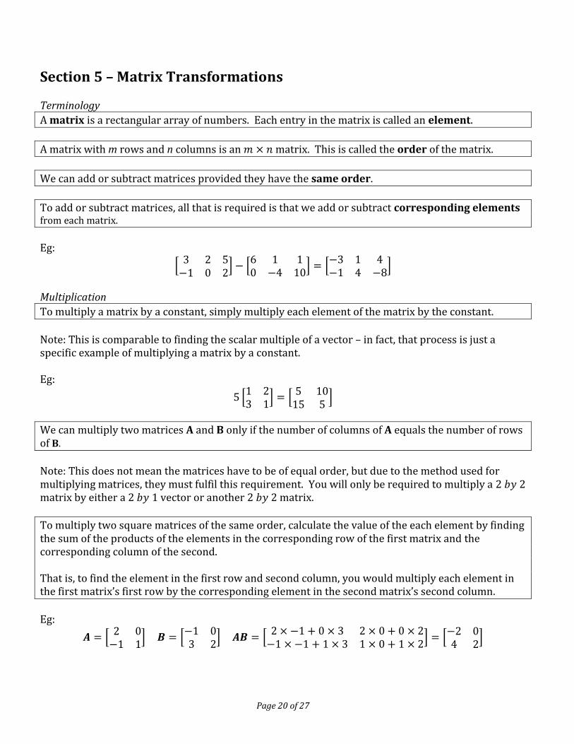
To multiply two square matrices of the same order, calculate the value of the each element by finding the sum of the products of the elements in the corresponding row of the first matrix and the corresponding column of the second. That is, to find the element in the first row and second column, you would multiply each element in the first matrix’s first row by the corresponding element in the second matrix’s second column.

Eg:

𝑨 = [2 0

−1 1] 𝑩 = [

−1 03 2

] 𝑨𝑩 = [2 × −1 + 0 × 3 2 × 0 + 0 × 2

−1 × −1 + 1 × 3 1 × 0 + 1 × 2] = [

−2 04 2

]

Page 21 of 27

In general, 𝑨𝑩 ≠ 𝑩𝑨. Matrix multiplication is not, in general, commutative. Note: Despite this, you will find that, in the limited case of some of the transformation matrices you will see, the order does not make a difference.

There is a square matrix 𝐼 with the property that 𝐼𝐴 = 𝐴𝐼 = 𝐴 for any compatible matrix 𝐴 (that is, square, and with the same order as 𝐼). This matrix is known as the identity matrix. The 2 𝑏𝑦 2 identity matrix is:

[1 00 1

]

[𝟏 𝟎𝟎 𝟏

]

Identity matrix. Right remains right, up remains up.

[−1 00 1

]

Reflection in the 𝑦-axis. Right has become left, up remains up.

[1 00 −1

]

Reflection in the 𝑥-axis. Right remains right, up has become down.

[−1 00 −1

]

Rotation by 180° Right has become left, up has become down.

[0 11 0

]

Reflection in the line 𝑦 = 𝑥. Right has become up, up has become right.

[0 −11 0

]

Rotation by 90° anticlockwise. Right has become up, up has become left.

[0 1

−1 0]

Rotation by 90° clockwise. Right has become down, up has become right.

[0 −1

−1 0]

Reflection in the line 𝑦 = −𝑥. Right has become down, up has become left.

[𝑎 00 1

]

Enlargement by scale factor 𝑎 in the 𝑥 direction. Right is multiplied by 𝑎, up remains up.

[1 00 𝑎

]

Enlargement by scale factor 𝑎 in the 𝑦 direction. Right remains right, up is multiplied by 𝑎.

[𝑎 00 𝑎

]

Enlargement by scale factor 𝑎 from the origin. Right is multiplied by 𝑎, up is multiplied by 𝑎.

[𝑎 00 𝑏

]

Enlargement by scale factor 𝑎 in the 𝑥 direction and scale factor 𝑏 in the 𝑦 direction. Right is multiplied by 𝑎, up is multiplied by 𝑏.

Note: The matrices shown above all either rotate, reflect or enlarge with respect to the origin (or in lines through the origin). You need to be able to identify them and to generate them for yourself.

Page 22 of 27

Each column of a 2 𝑏𝑦 2 transformation matrix is the image of the corresponding column of 𝐼 (the identity matrix).

Eg:

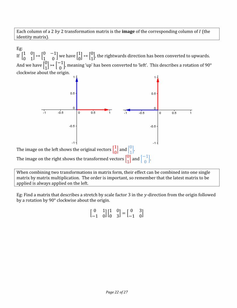
If [1 00 1

] ↦ [0 −11 0

] we have [10

] ↦ [01

], the rightwards direction has been converted to upwards.

And we have [01

] ↦ [−10

], meaning ‘up’ has been converted to ‘left’. This describes a rotation of 90°

clockwise about the origin.

The image on the left shows the original vectors [10

] and [01

].

The image on the right shows the transformed vectors [01

] and [−10

].

When combining two transformations in matrix form, their effect can be combined into one single matrix by matrix multiplication. The order is important, so remember that the latest matrix to be applied is always applied on the left.

Eg: Find a matrix that describes a stretch by scale factor 3 in the 𝑦-direction from the origin followed by a rotation by 90° clockwise about the origin.

[0 1

−1 0] [

1 00 3

] = [0 3

−1 0]

Page 23 of 27

Section 6 –Geometry

In addition to basic formulae for rectangles and triangles you should recall that the area of a triangle can be found using:

𝐴𝑟𝑒𝑎 =1

2𝑎𝑏 sin 𝐶

Where 𝑎 and 𝑏 are two lengths of the triangle and 𝐶 is the size of the angle in between.

For right-angled triangles, Pythagoras’ theorem applies: 𝑎2 + 𝑏2 = 𝑐2

Where 𝑎 and 𝑏 are the lengths of the two perpendicular sides and 𝑐 is the length of the hypotenuse.

For any triangle, whose sides are of length 𝑎, 𝑏 and 𝑐 with opposite angles 𝐴, 𝐵 and 𝐶 respectively:

𝑆𝑖𝑛𝑒 𝑟𝑢𝑙𝑒: 𝑎

sin 𝐴=

𝑏

sin 𝐵=

𝑐

sin 𝐶

𝐶𝑜𝑠𝑖𝑛𝑒 𝑟𝑢𝑙𝑒: 𝑎2 = 𝑏2 + 𝑐2 − 2𝑏𝑐 cos 𝐴

Note: The sine and cosine rule (as well as the general formula for area) are provided on the formula sheet (see the end of this booklet). You will need to be confident determining which to use and how.

To find area, first see if you can use 𝐴𝑟𝑒𝑎 =1

2𝑏ℎ. If not, try 𝐴𝑟𝑒𝑎 =

1

2𝑎𝑏 sin 𝐶.

To find a length, first see if you can use 𝑃𝑦𝑡ℎ𝑎𝑔𝑜𝑟𝑎𝑠 (triangle must be right-angled, and you will need to know two of the sides). If not, try 𝑆𝑖𝑛𝑒 𝑟𝑢𝑙𝑒 (you will need an opposite side and angle pair, plus the angle opposite your desired length). If not, try 𝐶𝑜𝑠𝑖𝑛𝑒 𝑟𝑢𝑙𝑒 (you will need the other two sides and the angle in between them). To find an angle, first see if you can use the 𝐴𝑛𝑔𝑙𝑒 𝑠𝑢𝑚 of triangles. If not, try 𝑆𝑖𝑛𝑒 𝑟𝑢𝑙𝑒 (you will need an opposite side and angle pair, plus the side opposite your desired angle). If not, try 𝐶𝑜𝑠𝑖𝑛𝑒 𝑟𝑢𝑙𝑒 (you will need all three sides).

Note: Sometimes you may need to apply a number of these rules to find what you want. If in doubt, use the simplest first and work out any unknown values you can, then reevaluate.

The ambiguous case can occur, usually when applying the sine rule, when calculating an angle. If we know the length of one side and the angle opposite, and one other side, we can find the 𝑠𝑖𝑛𝑒 of the angle opposite, but this may yield two equally valid possible solutions. Recall that sin 80 = sin 100, etc, so for every acute angle that the calculator will give, there is an alternative obtuse angle which can be found using 90 − 𝜃.

Page 24 of 27

Pythagoras’ theorem, and right-angled trigonometry may need to be applied in 3 dimensions:

For the angle between a line and a line: construct a triangle within the 3-D shape, and apply the normal rules.

For the angle between a line and a plane: drop a perpendicular line down to the plane from the line and form a right-angled triangle. The angle you want is between the side of the triangle which lies on the plane and your original line.

For the angle between a plane and a plane: find a line in each plane which is perpendicular to the line of intersection of the two planes. The angle between these lines is the angle between the planes.

The circumference of a circle is given by 𝐶 = 2𝜋𝑟 and the area by 𝐴 = 𝜋𝑟2. These formulae can be applied to sectors and segments as shown below: Sector Segment

Area:

𝐴 =𝜃

360𝜋𝑟2 𝐴 =

𝜃

360𝜋𝑟2 −

1

2𝑟2 sin 𝜃

Perimeter: 𝑃 =

𝜃

3602𝜋𝑟 𝑃 =

𝜃

3602𝜋𝑟 + 𝑟√2 − 2 cos 𝜃

Note: The more complicated-looking formulae for the segment do not need to be learned or even applied in this form – they are a combination of the area of a triangle formula and the cosine rule.

Know and be able to apply the following circle facts: A triangle with two corners on the circumference and one in the centre of a circle is

isosceles. A tangent and a radius always meet at right angles. The triangle formed by two tangents and the chord in between is isosceles. If a radius bisects a chord it does so at right angles, and vice versa.

Know, apply and quote the following circle theorems:

The angle at the centre of a circle is twice the angle at the circumference. The angle in a semicircle is a right angle. Angles in the same segment are equal. The sum of the opposite angles of a cyclic quadrilateral is 180°. The angle between a chord and the tangent is equal to the angle in the alternate segment.

Note: This final theorem can be quoted by name. Eg “By the Alternate Segment Theorem, 𝑥 = 30°.

Page 25 of 27

The 𝑠𝑖𝑛𝑒 function can be thought of as the height above the centre of a point moving around a circle. The 𝑐𝑜𝑠𝑖𝑛𝑒 function can be thought of as the distance to the right of the centre. The angle in question is the anti-clockwise angle from the 𝑥 axis as shown. Note that the height (the 𝑠𝑖𝑛𝑒 function) will be negative between 180° and 360°, and the distance to the right (the 𝑐𝑜𝑠𝑖𝑛𝑒 function) will be negative between 90° and 270°.

It is important to note that the functions sin 𝑥, cos 𝑥 and tan 𝑥 are valid not just for angles from 0° to 90°. Using the idea of the circle above, we can generate graphs for each function. Also, since it is possible to go as far clockwise or anticlockwise around the circle as you like, the function, and therefore graph, extends infinitely in both directions, but will simply repeat the first 360°.

𝑦 = sin 𝑥

𝑦 = cos 𝑥

𝑦 = tan 𝑥

Page 26 of 27

While approximate values for sin 𝑥 can be found using a calculator, sometimes exact values are useful. By cutting either an equilateral triangle or a square in half, we can use Pythagoras’ theorem to determine the exact lengths of the sides formed, and hence the exact values of a number of trigonometric ratios:

Angle Sine Cosine Tangent

0° 0 1 0

30° 1

2

√3

2

1

√3

45° 1

√2

1

√2 1

60° √3

2

1

2 √3

90° 1 0 (𝑢𝑛𝑑𝑒𝑓𝑖𝑛𝑒𝑑)

For any angle 𝜃:

tan 𝜃 =sin 𝜃

cos 𝜃

Note: This can be seen from the right-angled trigonometry formulae, since (

𝑜𝑝𝑝

ℎ𝑦𝑝)

(𝑎𝑑𝑗

ℎ𝑦𝑝)

=𝑜𝑝𝑝

𝑎𝑑𝑗

For any angle 𝜃: sin2 𝜃 + cos2 𝜃 = 1

Note: This can be seen by applying Pythagoras’ theorem to a standard right-angled triangle:

(𝑜𝑝𝑝

ℎ𝑦𝑝)

2

+ (𝑎𝑑𝑗

ℎ𝑦𝑝)

2

=𝑜𝑝𝑝2 + 𝑎𝑑𝑗2

ℎ𝑦𝑝2=

ℎ𝑦𝑝2

ℎ𝑦𝑝2= 1

Note: The two trigonometric identities above will be provided in the formula sheet.

To solve a trigonometric equation, first rearrange into the form sin 𝑥 = 𝑘 (eg sin 𝑥 = 0.5). Then find the principal value using a calculator (ie 𝑥 = sin−1 0.5 = 30°), then use the graph to find any other valid solutions within the range required. (eg 𝑥 = 30° or x = 150°).

Page 27 of 27

Appendix – Formulae Sheet In the exam you will be provided with a sheet of formulae just as in the GCSE exam, but with a few additions. The following is a list of the results you will be given:

𝑽𝒐𝒍𝒖𝒎𝒆 𝒐𝒇 𝒔𝒑𝒉𝒆𝒓𝒆 =4

3𝜋𝑟3

𝑺𝒖𝒓𝒇𝒂𝒄𝒆 𝒂𝒓𝒆𝒂 𝒐𝒇 𝒔𝒑𝒉𝒆𝒓𝒆 = 4𝜋𝑟2

𝑽𝒐𝒍𝒖𝒎𝒆 𝒐𝒇 𝒄𝒐𝒏𝒆 =1

3𝜋𝑟2ℎ

𝑪𝒖𝒓𝒗𝒆𝒅 𝒔𝒖𝒓𝒇𝒂𝒄𝒆 𝒂𝒓𝒆𝒂 𝒐𝒇 𝒄𝒐𝒏𝒆 = 𝜋𝑟𝑙

𝑨𝒓𝒆𝒂 𝒐𝒇 𝒕𝒓𝒊𝒂𝒏𝒈𝒍𝒆 =1

2𝑎𝑏 sin 𝐶

𝑺𝒊𝒏𝒆 𝒓𝒖𝒍𝒆: 𝑎

sin 𝐴=

𝑏

sin 𝐵=

𝑐

sin 𝐶

𝑪𝒐𝒔𝒊𝒏𝒆 𝒓𝒖𝒍𝒆: 𝑎2 = 𝑏2 + 𝑐2 − 2𝑏𝑐 cos 𝐴

cos 𝐴 =𝑏2+𝑐2−𝑎2

2𝑏𝑐

𝑻𝒉𝒆 𝒒𝒖𝒂𝒅𝒓𝒂𝒕𝒊𝒄 𝒆𝒒𝒖𝒂𝒕𝒊𝒐𝒏: 𝑇ℎ𝑒 𝑠𝑜𝑙𝑢𝑡𝑖𝑜𝑛𝑠 𝑜𝑓 𝑎𝑥2 + 𝑏𝑥 + 𝑐 = 0, 𝑤ℎ𝑒𝑟𝑒 𝑎 ≠ 0, 𝑎𝑟𝑒 𝑔𝑖𝑣𝑒𝑛 𝑏𝑦:

𝑥 =−𝑏 ± √𝑏2 − 4𝑎𝑐

2𝑎

𝑻𝒓𝒊𝒈𝒐𝒏𝒐𝒎𝒆𝒕𝒓𝒊𝒄 𝒊𝒅𝒆𝒏𝒕𝒊𝒕𝒊𝒆𝒔:

tan 𝜃 =sin 𝜃

cos 𝜃 sin2 𝜃 + cos2 𝜃 = 1

Produced by A. Clohesy; TheChalkface.net

13/06/2015