AD-A109 902 SCIENCE APPLICATIONS INC MCLEAN VA F/G 4/2NEAR-INERTIAL NOTIONS: A PRELIMINARY MOOL-DATA COMPAPISON, 0)JAN A2 D RUBENSTEIN NO0014-AI-C-n084

UNCLASSIFIED SAI-82-620-WA NL

II r IIII/EEN

Aprvdfo u~ rlce

NEAR-INERTIAL MOTIONS: A PRELIMINARY

MODEL-DATA COMPARISON

SAI-82-620-WA

IP

.- g

XATLANTA ANN AIOA * mOSTON * CI1CAGO • CLr4RMLA/n e DI HUNT$VL LA JOLUATIU ROC= e LOS ANELUS IAN S ANS • SANTA WARSANA • rUCSoN o WAHDIT

w

NEAR-INERTIAL MOTIONS: A PRELIMINARY

MODEL-DATA COMPARISON

SAI-82-620-WA J

TR-OPD-81-274-10

January 1982

Prepared by:

David RubensteinOcean Physics Division

Prepared for:

Naval Ocean Research and Development ActivityNSTL Station, Mississippi 39529!

IFinal Report for Contract No. N00014-81-C-0084and Technical Report for No. N00014-81-C-0075I

I SCIENCE APPLICATIONS, INC.

1710 Goodridge DriveP.O. Box 1303McLean, Virginia 22102(703) 821-4300

1 '71.,.,'.,.,'. I] l] "

-'4.. - .--

UNCLASSIFIED, C,..SS'C'CAOIN C1 TmIS PAE (.'.n Dos £nteredj

REPORT DOCUMENTATION PAGE ACESIO CSOMPLLTVUC FORM

!. " A;: I, - - . ,0 . G O V T A C C ES S IO N N O .' 3 . R E C IP IE N T C A T A L O G N U M 3 E R

Ner-Inr. l otn.:s:A 1. TYPE OF REPORT & PERICZ COVERED

Near-inertial Motions: A Preliminary Technical ReportModel-Data Comparison May - October 1981

6. PERFOP.,iNG ORS. REPORT NUMBER

SAI-82-620-WA7. A-;OP.'af 8. C7hTRACT OR GRANT NUMBER(o)

David Rubenstein N00014-81-C-0075N00014-81-C-0084

. C ZAN:ATIO NAME .NO ADDR:qS 10. PROGRAM ELEM NT. PROJECT. TASKAREA & WORK UNIT NUMBERS

Science Applications, Inc.1710 Goodridge DriveMcLean, VA 22102 1_1

i. COTR"t...,xG OFFICE NAME AND ADORESS 1Z. REPORT DATE

NORDA Code 540 January 1982Ocean Measurements Program 13. NUMS-RROFPAGESNSTL Station, Bay St. Louis, MS 39529

I-. MCNiT7 p.;h* ,-SCY NAME A ADD:RAS-Ul dilfern firt C ontro:|ns Office) IS. SECURITY CLASS. (OI lIe report)

UNCLASS I FIEDSame

13.. DECL ASSI F1 IATIONI OOWNGRADINGSCMEDULE

Approved for public release; distribution unlimited

=!S7P-SVT ION S7. AT EMEN7 (of --ho absr.cr etered in &for~k 20. it dI!I.,wif from Report;

Same

Ei. SUpp,_EN-AAY NOTES

1 . ,EY *"ft ,C nt on oeler d i nee ..ai. end don ty by block nunbor)

Inertial oscillationsShearf Ocean Modeling

: t . A T fC. onwn o. to*,*e . sde it necessary and Idenify by block number)

A summary of a wind-forced dynamical model of near-inertialmotions is presented. Results from this model are brieflyreviewed. Observations of coherence and response between windstress and upper ocean currents are compared with model results.

rD , '2- 1473 EoTION o, ,VS IoS$, ossoLETE UNCLASSI FIED

a. ___'. __"_. __,_. ____.____.______........ . ... ..___

!

TABLE OF CONTENTS

Page

List of Figures ....................................... ii

Section 1 INTRODUCTION ................................. 1-1

Section 2 BRIEF MODEL DESCRIPTION ..................... 2-1

Section 3 RESPONSE FUNCTION COMPUTATIONS ............. 3-1

3.1 General Considerations ................ 3-1

3.2 Model Response ......................... 3-3

3.3 Response Computed from CurrentMeter Records .......................... 3-4

Section 4 PRELIMINARY MODEL-DATA COMPARISONS ......... 4-1

4.1 General Remarks ........................ 4-1

4.2 Descriptive Comparison ................. 4-4

4.3 Quantitative Comparison ............... 4-11

4.4 Conclusions and Future Work ........... 4-15

References ............................................ R-1

AoN~~lForNTIS G:&I

PTT? -'.

*W .. .. . . --- . .

-Ac

es i For /o

A v G , ; c \ k 3

COPY

fNSE~CT~f,

LIST OF FIGURES

Page

Figure 4.1 Vaisala frequency at three mooringsin the upper l00 m ......................... 4-2

Figure 4.2 Profiles of Vaisala frequency andeddy diffusivity used in numericalmodel runs .................................. 4-3

Figure 4.3 Numerically computed responseamplitude function for shear at25 m ...................................... 4-5

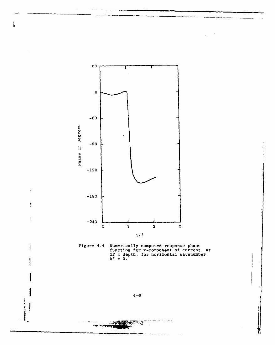
Figure 4.4 Numerically computed response phasefunction for v-component of current,

at 12 m ..................................... 4-6

Figure 4.5 Coherence amplitude, phase, andgain (response amplitude) functionscomputed between wind stress(#3391) and 12 m current (#3393) .......... 4-8

Figure 4.6 Coherence amplitude, phase, andgain (response amplitude) functionscomputed between wind stress(#3401) and 12 m current (#3402) .......... 4-10

Figure 4.7 Coherence amplitude, phase, andgain (response amplitude) functionscomputed between wind stress(#3391) and current meter velocitydifference (#3393-#3394) ................... 4-12

Figure 4.8 Comparison between observed andsimulated gain functions, betweenwind stress and 12 m current .............. 4-14

Figure 4.9 Comparison between observedand simulated shear gain functions ........ 4-16

I

i o i

!.

I

Section 1

INTRODUCTION

$ Pollard and Millard (1970) presented a mixed layer

model of near-inertial frequency wind-induced current. This

simple model is capable of simulating some of the important

aspects of the response of inertial currents to wind stress.

Kundu (1976) and Pollard (1980) also used this model, and

showed comparisons with current meter data. The model has

two parameters, a surface layer depth parameter and a linear

decay rate parameter. By adjusting the parameter values,

Kundu and Pollard optimized the agreement between the model

and current meter data. Most of the inertial motions were

shown to be linear responses to the wind-induced surface

stress.

Krauss (1981) modeled the wind-induced response

in the Baltic Sea, using a semispectral model. Krauss'

model allows the specification of depth dependent profiles

of eddy diffusivity and stratification. Krauss compared his

model results with current meter data, and found that the

erosion of the thermocline was due to the strong shear

associated with inertial waves.

In many respects, the model we developed is

quite similar to that of Krauss. In a previous report

(Rubenstein, 1981b) we presented the mathematical details of

our linear semispectral model. The equations are nearly the

same as those from Krauss (1981), but the method of solution

is much different. We solve the equations spectrally in the

spatial dimensions and numerically in time. As a result

1-1

A

of this difference in solution methods, we are able to

apply general, nonperiodic (in time) surface stress forcing

functions. This capability is advantageous, as it allows us

to emphasize the transient, time dependent nature of the

inertial response.

In a previous report (Rubenstein and Newman,

1981) we presented statistical analyses of current meter

data. These current meters were situated near Ocean

Site D (39 0 10'N, 70oW), and collected data for about

48 days during the summer of 1970. Three moorings each

held horizontal current meters at depths of 12, 32, 52,

and 72 m, and also wind velocity recorders. Current and

wind velocity were sampled at 15 minute intervals. The

moorings were positioned roughly 50 km apart from each

other. Additional details concerning the data set may be

found in Pollard and Tarbell (1975) and in Pollard (1980).

In this technical note we report a preliminary

assessment of our dynamical model. We do this by comparing

results from our model with statistics from the current

meter data. In particular, we compare the response spectra

of current and shear to an imposed wind stress.

In Section 2 we summarize our dynamical model.

We present the equations of motion and boundary conditions

and briefly outline the method of solution. In Section

3 we discuss the methods used to compute the response

functions. In Section 4 we compare the response functions

from the model and the current meter data. We discuss these

comparisons and speculate upon their implications.

1-2

-' v -. '-.,

f

Section 2

BRIEF MODEL DESCRIPTION

In this section we present the model equations

and an outline of their method of solution. The interested

reader is referred to Rubenstein (1981a) for a derivation of

the equations, and to Rubenstein (1981b) for a complete

description of their method of solution.

We consider a Boussinesq, hydrostatic ocean

contained in a flat bottomed channel. The channel is of

finite width and infinite length. The x-coordinate is

aligned across the width, the z-coordinate is positive

upwards. Table 2.1 is a list of the variables. The

asterisks indicate that they are dimensional. The equations

are listed below.

au -P u* uS fv* = + - (2.1)at x az* az"

av + fu* = *afu-- - , " (2.2)

at az (2.2)ii *

= - +(2.3)az

ab 2ab + N*2w 0, (2.4)

S* •au aw 0 (2.5)

ax Dz

2-1

7t

I

Table 2.1

DEFINITIONS OF VARIABLES

x*, y*, z* Right-handed coordinate system, z* pos-

itive up, z* = 0 at bottom, D at surface.

u*, v*, w* Velocity components

t* Time

P* P' Po, where p' is pressure fluctuation

from a reference state, and Po is arepresentative value of density

Eddy diffusivity, a function of z* only

N* Vaisala frequency;

N*2 = - (g dPr), where

Pr(z*) is a reference state of density.

b* Buoyancy; - p'g/po, where p' is densityfluctuation from a reference state.

2-2

!1

~ .~v.

Here, we have set to zero all derivatives with respect

to y*. We have also neglected the buoyancy eddy dif-

fusivity. term and the processes which maintain the buoyancy

profile against diffusion. The boundary conditions are as

follows.

w = 0 at z = 0, D, (2.6)

* -u =Du i v - 0 at z =0, (2.7)

az z

(,a - , at z =D, (28)

u = 0 at x = 0, L. (2.9)

The surface stress vector T*(X*,t*) is a pre-

scribed function which drives the system. Equations (2.6)

and (2.9) state that velocities normal to the channel

boundary surfaces should vanish. Equation (2.7) prescribes

that the stress, and therefore the shear at the bottom

should be zero. This boundary condition allows slippage at

the bottom.

The equations are nondimensionalized and combined

into two coupled equations in v and w. Approximate solu-

tions are sought in the form of truncated Fourier-Chebyshev

expansion; M N

V =E E Vjk(t)T(z) sin kwx (2.10)

k=l j'=0

M N

1: 2: Wjk(t)Tj(z) cos krx (2.11)

k=1 j=O

2-3

- V. n- .'l mlU I

The functions Tj(z) are j-order Chebyshev polynomials. The

boundary conditions are satisfied by using the Tau method,

discussed at great length by Gottlieb and Orszag (1977).

With this method, the highest order behavior of the solution

is determined not by the dynamical equations, but by the

boundary conditions.

The resulting differential equations are first

order in time for Vjk(t), and second order for Wjk(t). The

second order equation is split into two first order equa-

tions. Starting initially from rest, these ordinary dif-

ferential equations are then marched forward in time using a

third order (three-step) Lax-Wendroff scheme. After numeri-

cally integrating the differential equations, (2.10) and

(2.11) are expanded to give v and w as functions of x, z,

and t. The continuity equation (2.5) is then used to obtain

u(x,z,t).

2-4

I i

Section 3

RESPONSE FUNCTION COMPUTATIONS

3.1 GENERAL CONSIDERATIONS

We are interested in comparing the response

functions predicted by the dynamical model with the response

functions computed using the current meter data.

We let q represent some dynamical vector quantity,

such as current or shear. We assume that q(x,z,t) is alinear response to the wind stress, T (x,t). The Fourier

transforms of q and T in horizontal wavenumber k and angular

frequency w space are written Q(k,z,w) and r (k,w), and are

related byQ(k,z,w) = H q(k,z,w) r(k,w) . (3.1)

fq is the complex-valued response function which relates q

to the wind stress. This function may be decomposed into

two parts;

Hq (k,z,) = IH (k,z,w)j exp [ioq(kz,w)] (3.2)

where the amplitude Hq(k,z,w)I is sometimes called the gainfunction, and Oq(k,z,w) is the phase.

Following the notation in Bendat and Piersol(1971), we define the Fourier transforms in frequency over a

finite duration T to be

3-1

f

T

Q(M) = f q(t)e - iwt dt,

0T (3.3)

r(w) = t(t)e - i t dt, (3.4)

0

The one-sided power spectrum estimates are written

G (W) 2 2q() T IQ(w) I , (3.5)

2 2G () = - Ir(w)l (3.6)

T T

The cross spectral estimate is written

qT 2) = 2 Q*() r() (3.7)

where the asterisk indicates a complex conjugate. Note that

the auto spectra are real-valued, but the cross spectrum is

complex-valued. The gain function and phase are given by

IHq (w)l = IGqT(W)I

G (w) (3.8)

Im G QT (W

Oq (wA) - tan 1 R T( 39

We can also write the coherence amplitude;

G (W)qT (3.10)C(w) =- ____

GW) G_(w)q TF

3-2

A few comments concerning the interpretation

of coherence and response functions may be helpful to

the reader. When these functions are computed, an implicit

assumption is made, namely, that the system responds

linearly to the input (driving) function. In the absence

of contaminating noise, the response function is simply

the ratio of the output Fourier transform to the input

Fourier transform.

In the presence of contaminating noise, the

response function is the ratio of the cross-spectral density

function to the input spectral density function. Consider

an ensemble of N estimates of the input and output Fourier

transforms, i(w) and Qi(w), i = 1,...,N. For any partic-

ular frequency bin w+ L, we can plot sampled values of

Qi( ) vs. ri(O). In analogy with regression analysis,

the slope of the best-fit line through these sample points

is given by the gain in (3.8). The coherence amplitude in

(3.10) is a measure of the contaminating noise, and is

directly analogous to a linear correlation coefficient.

3.2 MODEL RESPONSE

In order to elicit a model response to a wind

stress, we drive the model with an impulse

AtY(x,t) = 6(t) sin k~rx (Pa/Pw) , (3.11)

where TY is the stress component in the y-direction.

The ratio of air density to water density, pa/Pw , allows us

to convert the wind stress to surface stress, which directly

drives the model.

3-3

W& To

-'9 '

fr

The limiting case of a delta function--infinite amplitude

and infinitesimal width--is not achievable using finite

differences. Instead we apply a sharp impulse 6(t) whose

integral is unity;

dt 1(3.12)

The Fourier transform of a delta function is unity. There-

fore the response function is simply given by

H (k,w) = G (k,w). (3.13)q q.

3.3 RESPONSE COMPUTED FROM CURRENT METER RECORDS

The frequency response of a current or a shear

time series to a wind stress is computed as follows. First,

the wind stress vector is computed using the standard

formulation

[ = Cd o IRo I (3.14)

where uo is the local wind vector, expressed in m/sec.

The drag coefficient is computed following Amorocho and

)DeVries (1980);

Cd = 0.0015 1 + exp J1 .56 + 0.00104. (3.15)1.56

Next, we follow the procedure described by

Gonella (1972) for computing vector coherence functions.

This procedure is outlined below.

1. Begin with two discrete vector time series, in

complex form;

F3-4

I

4.. '" • ,

-w . --' "

_(t n) T x (tn) + iry(tn)

u (tn) = u (tn) + iv (tn) ,

n = 0,1,..., L-1 (3.16)

Here, I = (TX , TY) is the vector wind stress, and u - (u,v)

is the current vector (or the difference between two ver-

tically separated current records).

The integer L is chosen7 to be an integer M multiple of N,

where N is a power of two:

L = MN . (3.17)

Divide each of the two time series into 2M-1 short Series,

overlapping one another by 50% and each of length N.

2. Multiply each of the short series by a Hanning

window function.

3. The two-sided Fourier transform (the transform is

not symmetric with respect to zero frequency) is computed

for each short complex series;

N-1r (fk = k) E (t n ) exp (-i2rkn/N)

n=O

N-i

(fk = E a (t n) exp (-i2kn/N)n-0

k= -N/2,..., N/2-1. (3.18)

3-5

- ... , - .

4. The auto, coincident, and quadrature spectral

density functions are computed:

Pl1 (f k) = <r (f k) * (f k)>

P 2 (f k) = <U (f k) U (f k)>

PI2 (fk - iQ1 2'(f k ) = <r (fk) U* (fk (3.19)

The asterisks denote complex conjugates, and the brackets

denote ensemble averages over the 2M-1 ensembles. This

procedure provides estimates with 2M degrees of freedom.

5. Compute the coherence amplitude, phase, and gain

(response amplitude), defined by

2/Ck ) P12 +12] 1/2

. . . . (3.20)P11 P22

)= arctan (Q1 2 /P1 2 ) (3.21)

,H(fk)i = 122 + Q122 1/2

P1 1 (3.22)

for frequencies fk = k/(tN), for k = - N/2.....N/2-1.

Negative frequencies indicate clockwise rotation and posi-

tive frequencies indicate counterclockwise rotation.

3I 3-6

F

Section 4

PRELIMINARY MODEL-DATA COMPARISONS

4.1 GENERAL REMARKS

In this section we present the coherence and

response functions of the current meter data, and compare

the response amplitude functions with those predicted by the

dynamical model. Prior to these presentations, it is

appropriate to make several comments concerning the validity

of the descriptive comparisons in Section 4.2 and the

quantitative comparisons in Section 4.3.

Figure 4.1 shows profiles of Vaisala frequency

in the upper 100 m, which were reported by Pollard (1980).

These profiles show a strongly stratified thermocline

centered at about 20 m, and weaker stratification below

about 40 m.

Figure 4.2 shows the smoothed profiles of Vaisala

frequency and eddy diffusivity that were used in the model

simulations. The Vaisala frequency profile is similar to

the profile observed at mooring 338 on July 23/24 1970,

shown in Figure 4.1. Below 90 m the profile has been

tapered to zero. The eddy diffusivity profile is patterned

after the one used by Krauss (1981).

The spatial distribution of the wind stress field

is an important aspect of our model-data comparisons.

Pollard (1980) analyzed the length scales associated

with the atmospheric front which passed Ocean Site D on

4-1

!~

BRUNT- VASAL, FREOUEnCY (cyclrs hcr)0 5 10 Is 20 25 30 35

.............30 JAY 9

'0 .

Figure 4.1 Vaisala frequency at the three moorings on 9and 23/24 July and 16/17 August as functionsof depth in the top 100 m. The profiles werecomputed using averaged values of density at

approximately 5 m intervals, so details of thestructure particularly in the top 15 m havebeen smoothed. From Pollard (1980).

4-2

I

-'--,

10

90

70-

60J

Z*(rn)"~r

3n

20 io10o I . I I i i i I i -

0 4 8 12 16 20 0 1 2 3 4 5 6N* (cph) *(M2 S- 1 )

Figure 4.2 Profiles of Vaisala frequency (left) andeddy diffusivity (right) used in numericalmodel runs.

II 4-3

II

August 11, 1970. The length scale along the direction

of propagation of the front is about 400 km, and the length

scale perpendicular to the propagation direction is about

40 km.

Unfortunately, not much more is known about

the spatial distribution of the wind stress field. The

dynamical model solves the horizontal spatial structure in

terms of Fourier modes. A quantitative comparison between

the model and observations requires knowledge of the wind

stress spatial distribution. In the absence of such

knowledge, we will have to make an assumption in Section 4.3

concerning the spatial power spectrum of wind stress. We

will assume that statistically, the predominant wind

stress contribution has an associated wavelength greater

than 300 km.

4.2 DESCRIPTIVE COMPARISON

Figure 4.3 shows the numerically computed response

amplitude of shear (from equations (3.5) and (3.13)). The

associated environmental profiles are shown in Figure 4.2.

The contour labels represent the relative amplitude levels,

at a depth of 25 m below the surface. The response ampli-

tude is greatly emphasized in a narrow band (between the

contours labeled 500) which coincides with the first verti-

cal mode dispersion relation. In Rubenstein (1981b), there

was evidence in the constant-stratification case of second

and third modes. Here too, there is also a slight hint

of an outline of the second vertical mode (in the region

bounded by the contour labeled 100, near w/f = 1.2,

k* = 0.3 km-1 ).

Figure 4.4 shows a numerically computed response

phase function. This example is for the response of the

4-4

i'~- -

f

2 100 50

f 500

2000 00

1

01-

0 .1 .2 .3 .4

k* (ki - 1)

Figure 4.3 Relative amplitude response of shear, forthe nonuniform stratification and eddydiffusivity profiles shown in Figure 4.2. Thechannel depth is 100 m. This figure shows theresponse at a depth of 25 m below the surface

j (z*/D = 0.75).

4-5

P- !M P

60 .

0

-60

bo

-90

-120

-180

-2400 1 2 3

Figure 4.4 Numerically computed response phasefunction for v-component of current, at12 m depth, for horizontal wavenumberk* 0.

4-6

4t

v-component of current, for horizontal wavenumber k* = 0.

The phase is nearly constant below the inertial frequency,

f. At the inertial frequency, the phase shifts sharply by

about 160 degrees. This behavior is characteristic of

resonant types of responses.

Rubenstein (1981b) developed, an analytic solution

to the initial start-up problem. The inviscid internal

waves equation was solved, subject to various formulations

of time dependent Ekman pumping boundary conditions. in a

uniformly stratified fluid, the resonant response amplitude

of vertical velocity to an impulsive driving force is

proportional to

2 f2w c -J j (4.1)wj ju.

where wj is the j'th eigenfrequency, and the index j is the

vertical mode number. As wj is inversely proportional to j,

the first mode j = 1 should be predominant. This result is

in agreement with Figure 4.3.

Using these insights, we can descriptively

evaluate the response functions of selectively chosen

current meter records. Figure 4.5 shows the coherence

amplitude, phase, and gain functions computed between the

wind stress measured by wind recorder #3391 and the current

measured by the current meter #3393, at 12 m depth. We

remind the reader that negative frequencies indicate clock-

wise vector rotation, and positive frequencies indicate

counterclockwise rotation. The most noticeable feature is

fthe strong peak in the gain function at the inertial

frequency, 0.0527 cph. The coherence amplitude at the

I4-7

ii"*

S ~ ~--E128 z:08 9

!z

-2;.Io -!,5.83 5 -5.27 2.00 5'.27 I10.5S 15.82 21.10 C'L " C "I .-

.10.

:' ,' :'E/628 a6 2 9

I\ /

cr E

I 1.5 .7 .0 5.7 -.58 .2 11

'h- cr

. F

•~~~V 0,) . 2

CSREC IC~ A'I Il cdu

c o

118 15.63 -'10.55 -5.27 8.0 5.27 10.55 15.82 21.1 leC

MIS.4

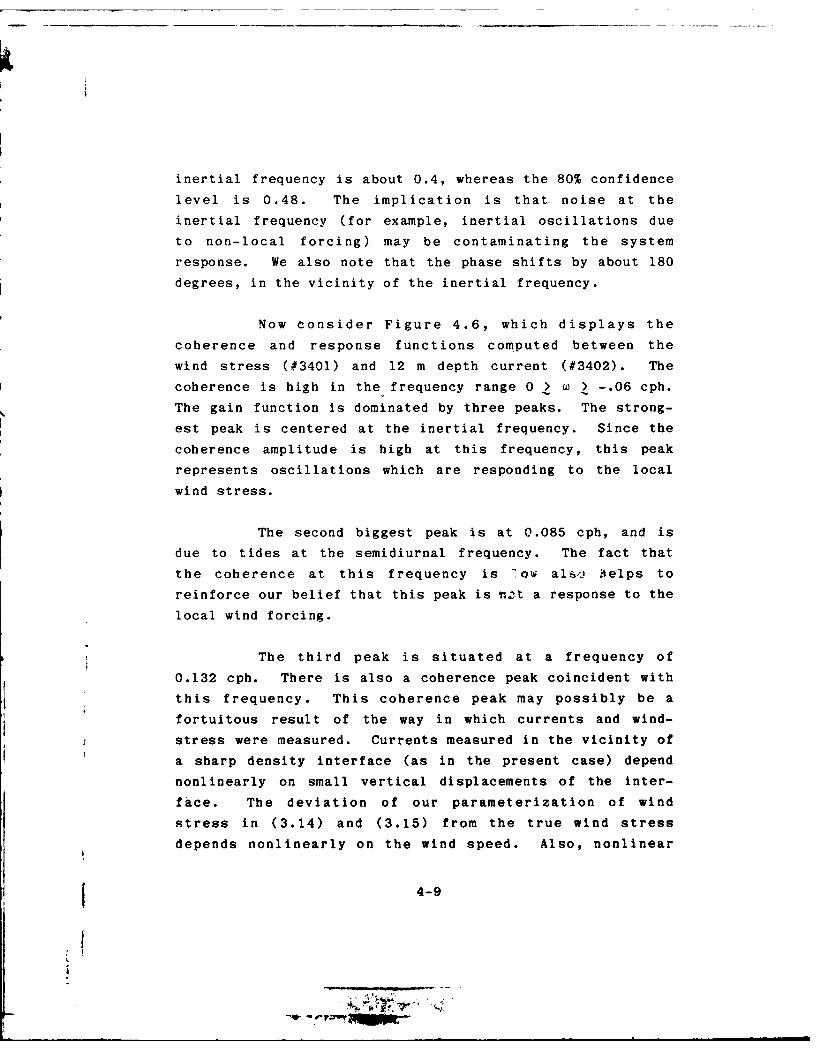
inertial frequency is about 0.4, whereas the 80% confidence

level is 0.48. The implication is that noise at the

inertial frequency (for example, inertial oscillations due

to non-local forcing) may be contaminating the system

response. We also note that the phase shifts by about 180

degrees, in the vicinity of the inertial frequency.

Now consider Figure 4.6, which displays the

coherence and response functions computed between the

wind stress (#3401) and 12 m depth current (#3402). The

coherence is high in the frequency range 0 > w > -. 06 cph.

The gain function is dominated by three peaks. The strong-

est peak is centered at the inertial frequency. Since the

coherence amplitude is high at this frequency, this peak

represents oscillations which are responding to the local

wind stress.

The second biggest peak is at 0.085 cph, and is

due to tides at the semidiurnal frequency. The fact that

the coherence at this frequency is "ow also, Aelps to

reinforce our belief that this peak is ntt a response to the

local wind forcing.

The third peak is situated at a frequency of

0.132 cph. There is also a coherence peak coincident with

this frequency. This coherence peak may possibly be a

fortuitous result of the way in which currents and wind-

stress were measured. Currents measured in the vicinity of

a sharp density interface (as in the present case) depend

nonlinearly on small vertical displacements of the inter-

face. The deviation of our parameterization of wind

stress in (3.14) and (3.15) from the true wind stress

depends nonlinearly on the wind speed. Also, nonlinear

4-9

3ZZ'.3422 6/28 A508 9

yvE

aP 1 0 -'15. 83 -IO.55 -5. 27 0 .00 5'.27 :0.55 15.802 21.18 0-

r'REC ICPHfl 010' 02

0 V-CL 02)

3ZO~~~0 3Z? -2 40

Vo E

~t2 6/2 4J8

C

E 0 v0

c05

4)-M

S-4

-2118-3.8 -8.5 -. 2 888 5. 27 38.55 35.82 2181FREG (CPHi 010

4-10

wind-induced motions of the surface buoy may be transmitted

through the mooring cable to the current meters. A combina-

tion of these unrelated nonlinear effects--in the wind

stress and in the measured response--may result in an arti-

ficial coherence peak, whose frequency is the sum of the

inertial and semidiurnal frequencies.

The vertical shear, computed by taking the

difference between pairs of vertically adjacent current

records, shows similar characteristics. As an example,

Figure 4.7 shows the coherence and response functions

between the wind stress (#3391) and the current meter pair

(#3393, 3394) located at 12 m and 32 m depth. Most striking

are the two peaks in the gain function, one at the inertial

frequency and the second at twice the inertial frequency.

Both peaks are associated with high coherence amplitude. In

analogy with the third spectral peak in Figure 4.6, the peak

in Figure 4.7 is possibly a fortuitous result of the way in

which currents and wind stress were measured.

The situation is further complicated by the

evidence for nonlinear interactions in power spectra of

currents and shears, discussed by Rubenstein and Newman

(1981). A number of these spectra show small peaks at the

frequency 0.132 cph, the sum of the inertial and semidiurnal

frequencies. This nonlinear interaction may feed energy

into the internal wave field, and may result in radiation

damping of the inertial oscillations in the mixed layer.

Unfortunately, our dynamical model is linear and is unable

to simulate such a process.

4.3 QUANTITATIVE COMPARISON

In this section we present quantitative com-

( parisons between the response amplitude (gain) functions

4-11

I

- , rmmr, _

3?9.B~3'394 5128 4608 9

7

WREQ~~' '-PH '

'43391.3393, 3394 6/26 A608 90 V0

-~ CIMCI

1w I)

W0)

V *C "

-2:.!0 -.5.93 -:2.55 -i.27 0'811 S.27 10.55 15.8? 21.10 - 4-

3~3:3933394 6/840 9CL54

4) -4-

t. 4J .W

4-1

predicted by the numerical model for horizontal current and

shear, and the average response amplitudes computed from

current meter observations. The purpose is not to show

exact agreement between theory and observations. Instead,

we show that the numerical solutions are of the correct

order of magnitude. Further fine tuning of the model should

be able to improve the agreement.

Figure 4.8 shows a comparison between the observed

and simulated gain functions. The solid curve represents

the average gain function for the three pairs of wind

recorders and uppermost current meters. This curve is a

mirror image about zero frequency, and represents the

clockwise rotary spectrum. The dashed curve labeled "A"

represents the simulated gain function between wind stress

and the current speed. The eddy diffusivity profile used

for this simulation is shown in Figure 4.2, and there is

no stratification. From the point of view of the model

equations, the statement that there is no stratification is

equivalent to the assertion that the wind stress does not

vary in space. In effect, we are assuming that the length

scale over which the wind stress varies is greater than

300 km. This assumption is supported by Pollard's (1980)

estimate that the horizontal wavelength of inertial oscil-

lations lies in the range 700-1700 km.

We see that the modeled response is too sharp;

the magnitude agrees at the inertial frequency, but in the

remainder of the frequency domain the model underestimates

the observed response function. By increasing the eddy

diffusivity profile by a factor of two (Case B), the

4-13

1

-MY

18

16

II'I

14 iI'

f i

8 1

I'I I

C.) Ii

I

o !t

0 1 I

I

00 -l -2 -3 -4

,,/f

Figure 4.8 Comparison between observed (solid line) andsimulated (dashed lines) gain functions. Gainis computed between wind stress and current at12 m depth. Eddy diffusivity profile used forCase A is shown in Figure 4.2, and Case B usesthe same profile, multiplied by a factor oftwo.

4-14

modeled response increases, but the sharpness of the

resonance remains the same.

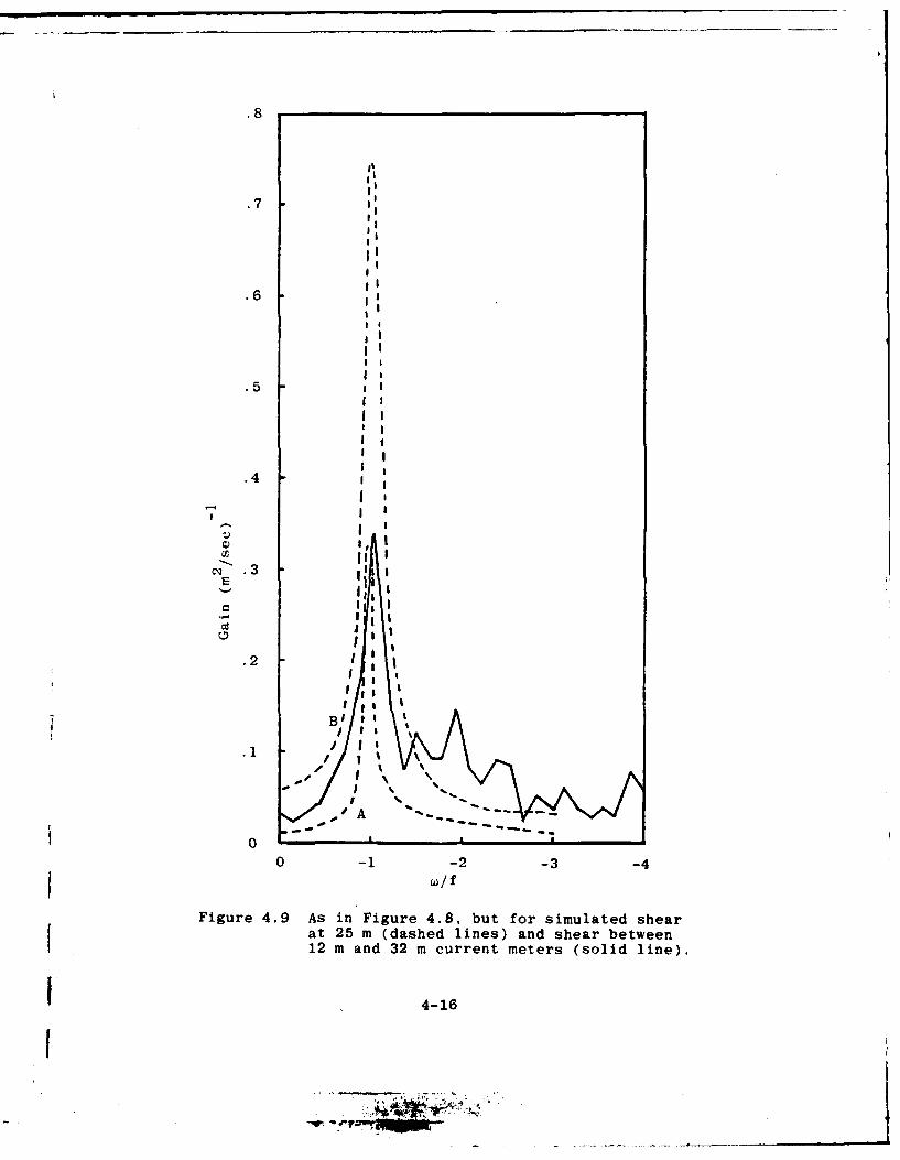
Figure 4.9 compares the observed response of

velocity difference to the modeled response of shear. The

comparison is very similar to the current response in Figure

4.8, and the same remarks apply here.

4.4 CONCLUSIONS AND FUTURE WORK

Krauss (1976) "showed that the shape of internal

wave resonances changes as the shape of the eddy diffusivity

profile is varied. The ratio of eddy diffusivity in the

surface layer to that in the interior is the most important

aspect of the profile shape. By varying this ratio, it

should be possible to fine tune our model, and to obtain

better agreement with the observed response. Our purpose

here is not to perform this fine tuning, but instead to show

that there is good general agreement between model and

observations. In SAI's Fiscal Year 1982 effort for NORDA's

Ocean Measurement Program, we plan to examine the sen-

sitivity of the model to variations in the eddy diffusivity

and Vaisala frequency profiles. After optimizing the

comparison of the response functions in the frequency

domain, we plan to extend the comparison into the time

domain.

The observations of response amplitude of current

and shear show peaks at the inertial frequency, and in some

cases at the semidiurnal tidal frequency and at somewhat

higher frequencies as well. The semidiurnal tidal peaks

4-15

KMWON

.8

.7i

.6

'Iii

I,

.5II II

I

.2 t

II A

III I

I I

I I

0 gl

02 2

I aI II ,s

B I

at I )

3 I

12 m nd3 mcrrntmtes(sli in)' A - - -.

4-1

0 -. -2 -3 -4t w/f

Figure 4.9 As in Figure 4.8, but for simulated shearat 25 m (dashed lines) and shear between

12 m and 32 m current meters (solid line).

I 4-16

I

cannot be predicted by our model of wind-induced shear. We

do not expect these peaks to be as significant in the open

ocean, far from regions of strong bottom topography.

We hypothesize that some fraction of the response

in the internal wave band (with frequency greater than

the inertial frequency) is due to transient atmospheric

events, such as fronts, whose horizontal length scales are

small. It may be possible to test this hypothesis through

further analysis of this set of current meter data, and

other data sets. Such- a test would entail comparisons

of the response functions computed during periods of intense

wind forcing events, with others during calm atmospheric

conditions. If these wind events have the shorter wave-

length components which are requisite for the excitation of

internal waves, then they will be associated with greater

spectral response in the internal wave band.

It may also be possible to test this hypothesis

using our dynamical model. This could be done by applying a

wind stress whose spatial dependence is more realistic than

the simplistic sinusoidal dependence in equation (3.11).

Wind stress patterns, whose spatial characteristics are

similar to fronts, could be applied to the model. The

response functions thus obtained should be more realistic in

the internal wave band than those plotted in Figures 4.8 and

4.9.

4-17

i

REFERENCES

Amorocho, J. and J.J. DeVries, 1980: A New Evaluationof the Wind Stress Coefficient Over Water Surfaces.J. Geophys. Res., 85, 433-442.

Bendat, J.S., and A.G. Piersol, 1971: Random Data:Analysis and Measurement Procedures, John Wiley andSons, Inc., New York.

Gonella, J., 1972: A Rotary-Component Method for AnalyzingMeteorological and Oceanographic Vector Time Series.Deep Sea Res., 19, 833-846.

Gottlieb, D. and S.A. Orszag, 1977: Numerical Analysisof Spectral Methods, Cambridge Hydrodynamics, Inc.,pp. 273.

Krauss, W., 1981: The Erosion of a Thermocline, J. Phys.Oceanogr., 11, 415-433.

Pollard, R.T., and R.C. Millard, 1970: Comparison BetweenObserved and Simulated Wind-Generated Inertial Oscil-lations. Deep-Sea Res., 17, 813-821.

Pollard, R.T., 1980: Properties of Near-Surface InertialOscillations, J. Phys. Oceanogr., 10, 385-398.

Pollard, R.T., and S. Tarbell, 1975: A compilation ofMoored Current Meter and Wind Observations, Volume VIII(1970 Array Experiment), Woods Hole Oceanographic Institu-tion, Ref. 75-7.

Rubenstein, D.M., 1981a: Models of Near Inertial VerticalShear. Science Applications, Inc., Ocean Physics Div.,McLean, VA.. SAI-82-564-WA.

Rubenstein, D.M., 1981b: A Dynamical Model of Wind-Induced Near-Inertial Motions. Science Applications,Inc., Ocean Physics Div., McLean, VA. SAI-82-598-WA.

Rubenstein, D.M., and F.C. Newman, 1981: Analysis andInterpretation of Shear from Ocean Current Meters.Science Appliations, Inc., Ocean Physics Div., McLean,VA. To be submitted.

R-1

____

-.

FIIE

DI