Approximation of Bit Error Rates in Digital

Communications

Graham V. Weinberg and Sharon Lee

Electronic Warfare and Radar DivisionDefence Science and Technology Organisation

DSTO—TN—0761

ABSTRACT

This report investigates the estimation of bit error rates in digital communi-cations, motivated by recent work in [6]. In the latter, bounds are used toconstruct estimates for bit error rates in the case of differentially coherentquadrature phase-keying with Gray coding over an additive white Gaussiannoise channel. By analysing Marcum’s Q-Function, which is an integral partof bit error rate expressions, we derive more direct methods of estimation,including least squares and truncated series approximations. Accurate andefficient estimates for bit error rates are then proposed.

APPROVED FOR PUBLIC RELEASE

DSTO—TN—0761

Published by

Defence Science and Technology OrganisationPO Box 1500Edinburgh, South Australia, Australia 5111

Telephone: (08) 8259 5555Facsimile: (08) 8259 6567

c Commonwealth of Australia 2007AR No. AR-013-930June, 2007

APPROVED FOR PUBLIC RELEASE

ii

DSTO—TN—0761

Approximation of Bit Error Rates in DigitalCommunications

EXECUTIVE SUMMARY

DSTO is a sponsoring partner in the Hypatia Scholarship scheme for mathematicallytalented women, and as such, through Electronic Warfare and Radar Division’s MicrowaveRadar Branch, sponsored the second author of this report to participate in a short researchproject through the Summer Vacation Scholarship Program. Named after the famousfemale mathematician Hypatia, the scheme provides both financial and mentoring assetsto encourage women to pursue their interests in the mathematical sciences. The workpresented here is a report on this project, jointly undertaken by Graham V. Weinberg andHypatia Scholar Sharon Lee, over the 2006/2007 Summer Period.

This project involves estimation of the Marcum Q-Function, which is an important tool indigital signal processing. It is of interest to both the radar and communications researchcommunities, and has been investigated by the first author quite extensively. Here weexamine bit error rate estimation in digital communications, which is intimately relatedto this function. We show that a method applied in a recent publication, which usesbounds to estimate bit error rates, can be improved considerably by using more directtechniques of estimation.

This work is relevant to the long range research efforts into radar detection issues associatedwith Task AIR 04/206, EWRD Support for AP-3C E/LM2022 Radar System. Althoughfocusing on a communications application, the results transfer directly to the latter. Thetechnique examined here will be useful for engineers and scientists looking for efficient andaccurate approximations for intractable integrals.

iii

DSTO—TN—0761

iv

DSTO—TN—0761

Authors

Graham V. WeinbergElectronic Warfare and Radar Division

Graham V. Weinberg, Ph.D. is a specialist in mathematicalanalysis and applied probability, and is a graduate of The Uni-versity of Melbourne. His major DSTO research interest hasbeen the mathematical and stochastic approximation and esti-mation of radar performance measures.

Sharon LeeDSTO Summer Vacation Scholarship Program 2006/2007

Sharon Lee is a recipient of the 2005 Hypatia Scholarship formathematically talented women, studying a Mathematical andComputer Modelling degree at the University of South Aus-tralia.

v

DSTO—TN—0761

vi

DSTO—TN—0761

Contents

1 Introduction 1

1.1 Bit Error Rates and Marcum’s Q-Function . . . . . . . . . . . . . . . . . 1

1.2 Integral Representations of Marcum’s Q-Function . . . . . . . . . . . . . 2

1.3 Least Squares Method . . . . . . . . . . . . . . . . . . . . . . . . . . . . . 3

1.4 Contributions of this Report . . . . . . . . . . . . . . . . . . . . . . . . . 3

2 Numerical Approximation Schemes 5

2.1 Least Squares on a Finite Interval . . . . . . . . . . . . . . . . . . . . . . 5

2.1.1 An Estimator Based on Integral Representation (6): E1 . . . . . 5

2.1.2 An Approximation Based on Integral Representation (5): E2 . . . 6

2.2 Least Squares on a Semi-infinite Interval: E3 . . . . . . . . . . . . . . . . 7

2.3 Polynomial Integrand Approximations . . . . . . . . . . . . . . . . . . . . 7

2.3.1 An Estimator Based on Integral Representation (6): E4 . . . . . 8

2.3.2 An Approximation Based on Integral Representation (8): E5 . . . 8

2.3.3 An Estimator Based on the Transformed Integral Representation:E6 . . . . . . . . . . . . . . . . . . . . . . . . . . . . . . . . . . . 8

2.4 Taylor Series Approaches: E7 . . . . . . . . . . . . . . . . . . . . . . . . . 9

3 Performance Analysis 10

3.1 LS Estimators E1, E2 and E3 . . . . . . . . . . . . . . . . . . . . . . . . . 10

3.2 LS Estimators E4, E5 and E6 . . . . . . . . . . . . . . . . . . . . . . . . . 10

3.3 Taylor Series Estimator E7 . . . . . . . . . . . . . . . . . . . . . . . . . . 11

3.4 Time Performance Analysis . . . . . . . . . . . . . . . . . . . . . . . . . . 12

4 Conclusion 13

5 Acknowledgements 13

vii

DSTO—TN—0761

6 References 14

Appendix A: Comparision Plots of the Estimators 17

Appendix B: Tables of Numerical Results 25

viii

DSTO—TN—0761

Figures

A.1 A plot comparing E1 and ASQ for the region γ = 0dB to γ = 12dB. TheBER is given in a logarithmic scale. Observe that estimator E1 performs wellfor small values of γ, specifically where γ ≤ 6dB. . . . . . . . . . . . . . . . . 17

A.2 Performance of E2 in comparision with ASQ on the interval γ = 0dB toγ = 8dB. The BER is given in a logarithmic scale. Estimator E2 providesgood approximation for γ ≤ 5dB, with increasing accuracy for smaller SNRvalues. . . . . . . . . . . . . . . . . . . . . . . . . . . . . . . . . . . . . . . . . 18

A.3 A plot displaying the performance of E3 in comparision to ASQ for γ = 0dBto γ = 12dB. The BER are given in a logarithmic scale. Estimator E3performs well for larger values of γ, in particular, γ ≥ 10dB. Observe thataccuracy increases as the SNR increases. . . . . . . . . . . . . . . . . . . . . . 18

A.4 A Comparison of the three estimators E1, E2 and E3, with ASQ. . . . . . . . 19

A.5 Performance of E4 in comparision with ASQ on the interval γ = 0dB toγ = 10dB. The BER is given in a logarithmic scale. Notice that for γbeyond 8dB, E4 begins to deviate from ASQ. Estimator E4 provides goodapproximation for the region γ ≤ 8dB, with increasing accuracy for smallerSNR values. . . . . . . . . . . . . . . . . . . . . . . . . . . . . . . . . . . . . . 19

A.6 A plot comparing E5 and ASQ for the region γ = 0dB to γ = 12dB. Observethat E5 covers ASQ. For the range of γ values of interest, approximation E5provides good results. High accuracy approximations are obtained for γ ≤ 9dB. 20

A.7 Performance of E6 in comparision with ASQ on the interval γ = 0dB toγ = 12dB. The BER is given in a logarithmic scale. Approximation E6performs extremely well on the region of interest, providing high accuracyresults for γ ≤ 12dB. . . . . . . . . . . . . . . . . . . . . . . . . . . . . . . . . 20

A.8 A Comparison of the three estimators E4, E5 and E6, with ASQ. . . . . . . . 21

A.9 A comparison plot of E6 using n = 6, (3), (4) and ASQ for γ = 0dB toγ = 14dB. The BER is given in a logarithmic scale. Estimator E6 with n = 6performs extremely well on this region, providing extremely high accuracyresults. Observe that E6 with n = 6 is almost exactly on ASQ. . . . . . . . . 21

A.10 An enlarged view of Figure A.9 around γ = 13. Note that BER using (4) fallsoutside the region of the Figure. Observe how closely E6 approximate ASQ. 22

A.11 A plot of E7 and ASQ for γ = 0dB to γ = 12dB. The BER is given ina logarithmic scale. Extremely high accuracy results is obtained using theseries in (26) for the entire region of interest. . . . . . . . . . . . . . . . . . . 22

ix

DSTO—TN—0761

A.12 Time performance plot of E6, E7 and ASQ. Time is in seconds and accu-racy is given in a logarithmic scale, base 10. Observe that both E6 and E7are extremely efficient in comparision with ASQ. Both E6 and E7 are veryconsistent, while ASQ depends heavily on the degree of accuracy. . . . . . . . 23

A.13 An enlarged view of Figure A.12 at 10−15, suggesting E6 is more efficientthan E7. Note that ASQ falls outside the region of the Figure. . . . . . . . . 23

x

DSTO—TN—0761

Tables

B.1 A comparision of E1 and ASQ approximations, with a tolerance of 10−18.Five equally spaced points are used for fitting the modified Bessel function.

1 represents the absolute error between E1 and ASQ, and 2 is the relativeerror . . . . . . . . . . . . . . . . . . . . . . . . . . . . . . . . . . . . . . . . . 25

B.2 Approximations of BER(γ|a, b) based on estimator E2 on the interval γ =0dB to γ = 8dB. Five equally spaced points are used for fitting the modifiedBessel function. 1 = |ASQ−E2| and 2 = 100× 1

ASQ . . . . . . . . . . . . . . 25

B.3 A comparision of E3 with ASQ approximations. Five equally spaced pointsare used for fitting the modified Bessel function. 1 represents the relativeerror of E3 and 2 is the relative error. . . . . . . . . . . . . . . . . . . . . . . 26

B.4 Estimates of BER(γ|a, b) using E4 on the interval γ = 0dB to γ = 12dB. 100equally spaced points are used for fitting the intergand in (6). 1 = |ASQ−E4|and 2 = 100× 1

ASQ . . . . . . . . . . . . . . . . . . . . . . . . . . . . . . . . . 26

B.5 A comparision of the approximation of BER(γ|a, b) based on equation (20)with that obtained via ASQ. 50 equally spaced points are used for fitting theintergrand in (8). 1 = |ASQ−E5| and 2 = 100× 1

ASQ . . . . . . . . . . . . . 27

B.6 Performance of E6, (3) and ASQ. 1 represents the relative error of E6 and

2 is the relative error given in [5]. Observe that E6 outperforms (3). . . . . . 27

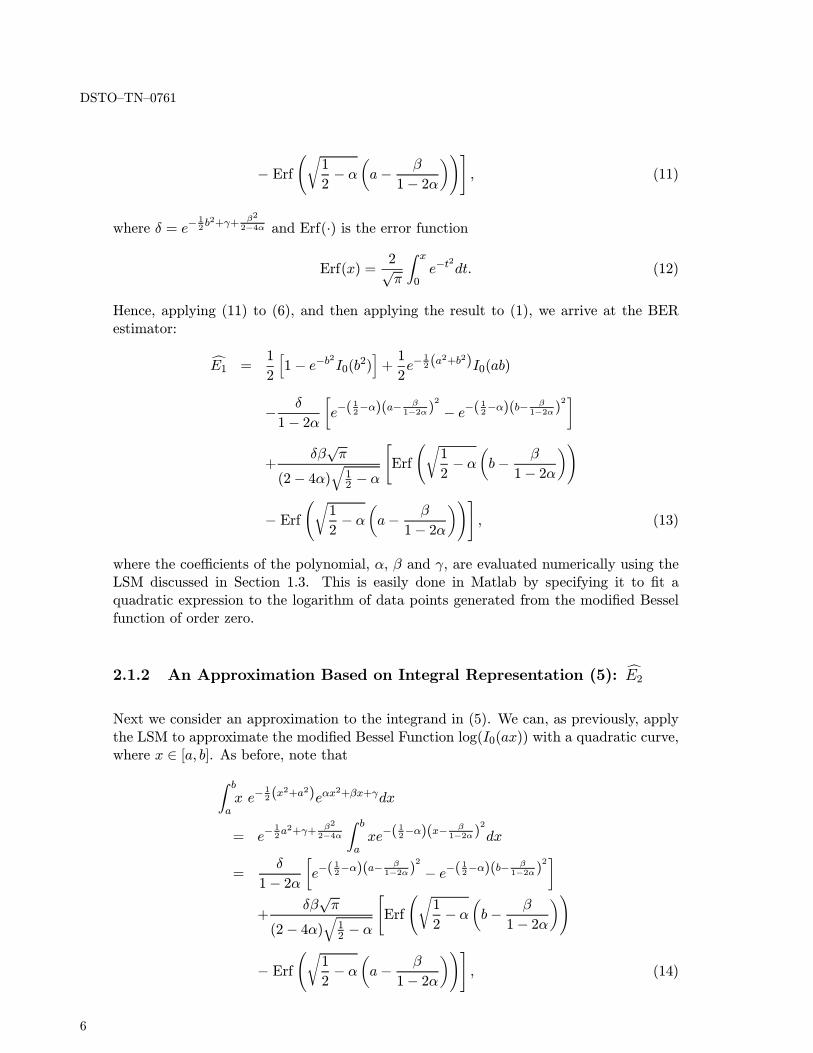
B.7 A comparision of E6 with n = 6, approximations using [6] and ASQ on theinterval γ between 0dB and 14dB. 1 represents the relative error of E6 withn = 6, 2 indicates the relative error of (3)and 3 is the relative error of (4).Notice the high degree of accuracy of E6 for small values of γ. . . . . . . . . . 28

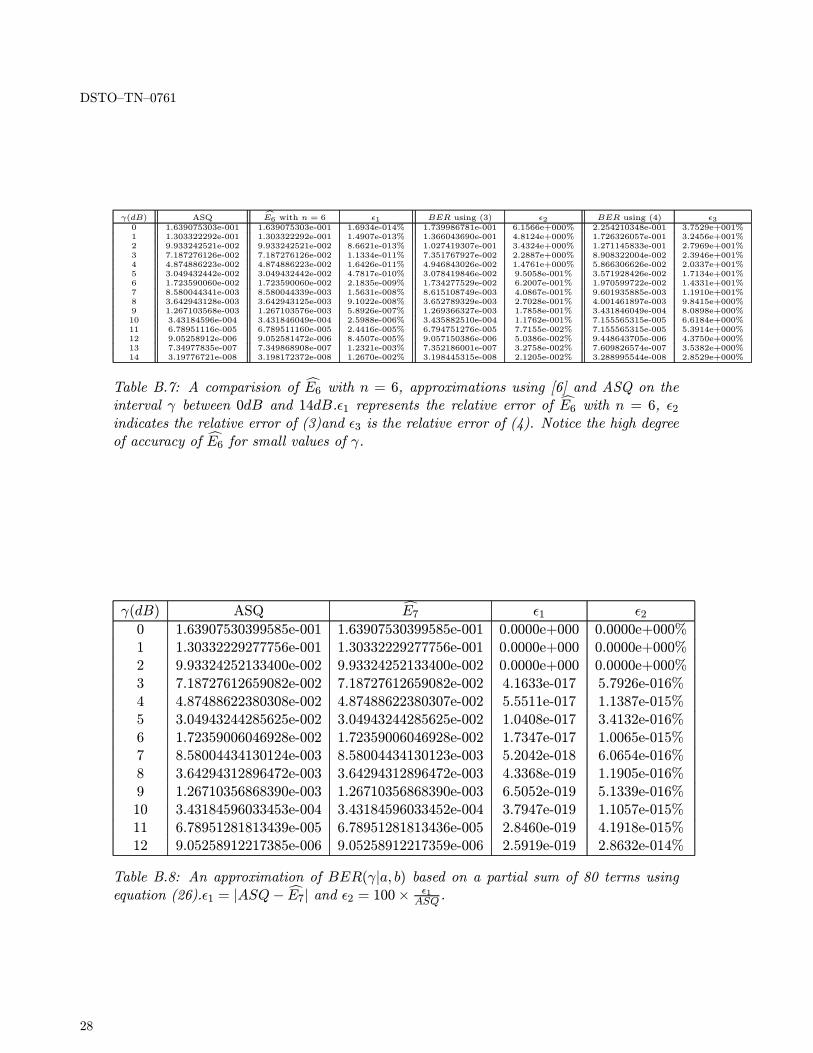
B.8 An approximation of BER(γ|a, b) based on a partial sum of 80 terms usingequation (26). 1 = |ASQ−E7| and 2 = 100× 1

ASQ . . . . . . . . . . . . . . . 28

B.9 Time performance of E6, E7 and ASQ. Time is given in seconds. Accuracy isgiven by 10−m, wherem ∈ {8, 9, . . . , 18}. Observe that E6 is the most efficientestimator, with E7 following closely behind. ASQ is the least efficient, andtime increases as the accuracy increases. Both E6 and E7 are very consistent. 29

xi

DSTO—TN—0761

xii

DSTO—TN—0761

1 Introduction

This report examines the estimation of bit error rates (BERs) in digital communications[1]. Specifically, we will investigate the recent work of [6] on using bounds to constructapproximations for differential quaternary phase shift keying (DQPSK) transmission withGray coding over an additive white Gaussian noise channel (AWGNC) [14]. In [6], anestimate of this BER is constructed by averaging a lower and upper bound. We showthat more direct methods can be applied to estimate the BER, and in some cases moreaccurate results are obtained.

The BER is a fundamental performance measure of a system, quantifying the reliabilityor integrity of a received signal [1]. The instantaneous BER, for many practical com-munication systems, in particular, wireless communications systems, can be written as afunction involving the standard Marcum Q-Function ([11], [12] and [13]). This famousfunction has received much attention in the digital signal processing literature, due to itsintractability. Hence, many estimation schemes have been proposed, employing techniquessuch as Adaptive Simpson Quadrature (ASQ) [10], Taylor Series approximations [16], theconstruction of lower and upper bounds ([4] — [9] and [19]) and the Monte Carlo scheme([23] and [24]).

1.1 Bit Error Rates and Marcum’s Q-Function

We specialise our analysis to the case considered in [6], as described above. In this scenario,the instantaneous BER is described by

BER(γ|a, b) := Q(a√γ, b√γ)− 12e−

12(a

2+b2)γI0(abγ), (1)

where constants a and b depend on the modulation/demodulation format, and γ is thetotal instantaneous signal to noise ratio per bit, and Q(α,β) is the standard MarcumQ-Function, defined by

Q(α,β) :=∞

βxe−

12(x

2+α2)I0(αx)dx, (2)

and I0(·) is the modified Bessel function of order zero. In the case considered in [6],

a = 2−√2 and b = 2 +√2, so that b > a. The key to estimating (1) is to construct

good approximations of (2).

Using lower and upper bounds on (2), derived in [5], one can show that

BER(γ|a, b) ≈ π

8

I0(abγ)

exp(abγ)

√γ(a+ b)Erfc

γ

2(b− a) , (3)

where Erfc is the complementary error function (see [6] for details).

1

DSTO—TN—0761

Using asymptotic approximations, [6] also proposed the following approximate expression,for large values of γ:

BER(γ|a, b) ≈ 1√8πab

b+ a

b− ae− − (b−a)2

2

=

√2 + 1

8π√2

1√γe[−(2−

√2)γ]. (4)

Although (3) and (4) produce good results, we will investigate a more direct approachto the estimation of the BER. The Least Squares (LS) approach is an interpolation tech-nique, which may be applied usefully to facilitate the estimation of (2). Additionally,we will consider Taylor Series approximations applied directly to (2). Before consideringestimators, we introduce a number of useful representations of the Marcum Q-Function.

1.2 Integral Representations of Marcum’s Q-Function

A number of new representations of (2) have been derived in [22]. In the spirit of [4],these convert the Marcum integral to one on a finite domain, with penalty terms added.Converting the Marcum integral (2) to one on a finite domain has the potential to improvethe estimation process, since it is somewhat easier to estimate an integral on a finitedomain.

It can be shown that

Q(a, b) =1

21 + e−a

2I0(a

2) +a

bxe−

12(x

2+a2)I0(ax)dx. (5)

Additionally, by an application of the symmetry relation [15] of the Marcum Q-Functionto (5), one can derive

Q(a, b) =1

21− e−b2I0(b2) + e− 1

2(a2+b2)I0(ab)

−b

axe−

12(x

2+b2)I0(bx)dx. (6)

Further details of the derivation of (5) and (6) can be found in [22].

It is, of course, not difficult to reduce (2) to an integral over a finite domain. Clearly wecan write

Q(a, b) = 1−b

0xe−

12(x

2+a2)I0(ax)dx. (7)

Also, one can apply the Marcum symmetry relation [15] to (7) to produce

Q(a, b) = e−12(a

2+b2)I0(ab)−a

0xe−

12(x

2+b2)I0(bx)dx. (8)

2

DSTO—TN—0761

We will construct a number of estimators based upon (5), (6) and (8), using the LeastSquares Method.

1.3 Least Squares Method

The Least Squares Method (LSM) [3] fits a smooth curve, with minimum error, to a givenset of data points. Error, in this case, refers to the sum of the squares of the errors(SSE) or the residuals of the points from the curve. To fit a polynomial of degree n,Pn(x) = αnx

n + αn−1xn−1 + · · ·+ α1x+ α0, to a set of m data points, where m ≥ n+ 1,the coefficients of the polynomial are determined such that the SSE is minimised, where

SSE =m

k=0

[Pn(xk)− yk]2 , (9)

and (xk, yk), k = 1, . . . ,m, are the data points.

The minimum SSE is obtained by taking the partial derivatives of (9) and equating themto zero. The resultant set of equations are known as the normal equations [3]. Thecoefficients are obtained by solving the normal equations.

α0n+ α1

m

k=0

xk + · · ·+ αn

m

k=0

xnk =m

k=0

yk

α0

m

k=0

xk + α1

m

k=0

x2k + · · ·+ αn

m

k=0

xn+1k =m

k=0

xkyk

· · ·

α0

m

k=0

xnk + α1

m

k=0

xn+1k + · · ·+ αn

m

k=0

x2nk =m

k=0

xnkyk. (10)

1.4 Contributions of this Report

This report explores the idea of applying LS approximations to evaluate the BER Function(1), achieved by estimating the Marcum Q-Function (2). Instead of applying bounds toestimate the Marcum Q-Function, as in [6], we show that more direct methods can beapplied to produce estimators. Specifically, six estimators can be constructed from thefinite interval representations of the Marcum Q-Function. In particular, three of theestimators use an exponential function with a quadratic polynomial power to estimate themodified Bessel function. The second group of three fit a polynomial of degree 5 to theentire integrand. These six estimators are compared to the results obtained from ASQ.Speed and accuracy performance are also analysed. We attempt to identify an optimal LSestimator.

3

DSTO—TN—0761

In addition, we examine a Taylor Series approximation of the BER function. Its perfor-mance is also compared with ASQ and the best performing LS estimator.

4

DSTO—TN—0761

2 Numerical Approximation Schemes

A number of estimators of the BER, based on the LS scheme and Taylor Series approach,are now introduced. The LS estimators are constructed by substituting functional ap-proximations to the integrands in (2), (5), (6) and (8). In some cases, the modified Besselfunction is approximated by an exponential function, while in others, we apply a polyno-mial approximation to the entire integrand. We also introduce a single estimator based

upon a truncated Taylor Series. Throughout we assume, as in [6], that a = 2−√2 andb = 2 +

√2, and hence b > a.

The key problem in terms of estimation of the Marcum Q-Function is the presence of themodified Bessel function in the integrand. Hence, we apply functional approximations toeliminate it from the integrand, to facilitate integration. Many of the proposed functionalapproximations suggested below have been produced by considering suitable fits to theBessel function by an appropriate polynomial. This will be done by using Least Squaresfits.

2.1 Least Squares on a Finite Interval

To begin, we consider approximating the modified Bessel Function with an exponentialfunction of the form f(x) = eαx

2+βx+γ on a specified finite interval. This is achieved byfitting a quadratic function, αx2+βx+ γ, to log(I0(x)), where the coefficients α, β and γare real constants. Applying the LS scheme, the coefficients can be determined using themethod outlined in Section 1.3. This scheme requires sequential estimation of the valuesof the modified Bessel Function. However, this is not viewed as a shortcoming becausethe tendency in the literature is to construct approximations of the integral (2) in termsof such functions anyway.

2.1.1 An Estimator Based on Integral Representation (6): E1

In view of (6), we can fit an exponential function to the modified Bessel function componentof the integral. Note that

b

ax e

12(x

2+b2)eαx2+βx+γdx

= e−12b2+γ+ β2

2−4αb

axe−(

12−α)(x− β

1−2α)2

dx

=δ

1− 2α e−(12−α)(a− β

1−2α)2

− e−( 12−α)(b− β1−2α)

2

+δβ√π

(2− 4α) 12 − α

Erf1

2− α b− β

1− 2α

5

DSTO—TN—0761

− Erf 1

2− α a− β

1− 2α , (11)

where δ = e−12b2+γ+ β2

2−4α and Erf(·) is the error function

Erf(x) =2√π

x

0e−t

2dt. (12)

Hence, applying (11) to (6), and then applying the result to (1), we arrive at the BERestimator:

E1 =1

21− e−b2I0(b2) + 1

2e−

12(a

2+b2)I0(ab)

− δ

1− 2α e−(12−α)(a− β

1−2α)2

− e−( 12−α)(b− β1−2α)

2

+δβ√π

(2− 4α) 12 − α

Erf1

2− α b− β

1− 2α

− Erf 1

2− α a− β

1− 2α , (13)

where the coefficients of the polynomial, α, β and γ, are evaluated numerically using theLSM discussed in Section 1.3. This is easily done in Matlab by specifying it to fit aquadratic expression to the logarithm of data points generated from the modified Besselfunction of order zero.

2.1.2 An Approximation Based on Integral Representation (5): E2

Next we consider an approximation to the integrand in (5). We can, as previously, applythe LSM to approximate the modified Bessel Function log(I0(ax)) with a quadratic curve,where x ∈ [a, b]. As before, note that

b

ax e−

12(x

2+a2)eαx2+βx+γdx

= e−12a2+γ+ β2

2−4αb

axe−(

12−α)(x− β

1−2α)2

dx

=δ

1− 2α e−(12−α)(a− β

1−2α)2

− e−( 12−α)(b− β1−2α)

2

+δβ√π

(2− 4α) 12 − α

Erf1

2− α b− β

1− 2α

− Erf 1

2− α a− β

1− 2α , (14)

6

DSTO—TN—0761

where δ = e−12a2+γ+ β2

2−4α . Hence, by applying (14) to (5), and by an application of theresult to (1), we arrive at the estimator:

E2 =1

21 + e−a

2I0(a

2) − δ

1− 2α e−(12−α)(a− β

1−2α)2

− e−( 12−α)(b− β1−2α)

2

−12e−

12(a

2+b2)I0(ab)

− δβ√π

(2− 4α) 12 − α

Erf1

2− α b− β

1− 2α

− Erf 1

2− α a− β

1− 2α . (15)

2.2 Least Squares on a Semi-infinite Interval: E3

An LS estimator is now proposed, based upon the original Marcum Q-Function (2). As inthe previous Subsections, we can apply a quadratic approximation to the logarithm of themodified Bessel function in the integrand of (2). By doing this, and applying the result to(1), we arrive at the estimator:

E3 =δ

1− 2α e−(12)−α(b− β

1−2α)2

−12e−

12(a

2+b2)I0(ab)

+δβ√π

(2− 4α) 12 − α

Erfc1

2− α b− β

1− 2α , (16)

where δ = e12a2+γ+ β2

2−4α and Erfc(·) is the complementary error function

Erfc(x) =2√π

∞

xe−t

2dt. (17)

Next we consider polynomial approximations of the entire integrand, using the LSM.

2.3 Polynomial Integrand Approximations

A number of polynomial approximations are now examined. In particular, we apply anapproximation with a polynomial of degree 5 to the entire integrand of the respectiveintegral.

7

DSTO—TN—0761

2.3.1 An Estimator Based on Integral Representation (6): E4

To begin, we apply this idea to the integrand of (6). In particular, xe−12x2I0(bx), can be

approximated by a fifth order polynomial, f(x) = α1x5+α2x

4+α3x3+α4x

2+α5x+α6,where x ∈ [a, b]. It can be shown that

e−12b2

b

aα1x

5 + α2x4 + α3x

3 + α4x2 + α5x+ α6 dx = e−

12b2 [g(b)− g(a)] , (18)

where g(t) = α16 t

6 + α25 t

5 + α34 t

4 + α43 t

3 + α52 t

2 + α6t.

Applying (18) to (6), then (1), results in the following estimator:

E4 =1

21− e−b2I0(b2) + 1

2e−

12(a

2+b2)I0(ab)− e− 12b2 [g(b)− g(a)] . (19)

The coefficients of the polynomial are estimated by the LSM in Matlab.

2.3.2 An Approximation Based on Integral Representation (8): E5

Using an argument similar to that as in the construction of (19), one can construct theestimator

E5 =1

2e−

12(a

2+b2)I0(ab) + e− 12b2g(a) (20)

based upon (8).

2.3.3 An Estimator Based on the Transformed Integral Representation:E6

Consider the transformation a =√2ς, b =

√2τ and v = x2

2 (see [22] for details of thistransformation) of the integral (8). By applying the transformation to (8) and (1), wearrive at the following expression for the BER:

BER(γ|ς, τ) = 1

2e−(τ+ς)I0(2

√τς) +

ς

0e−(v+τ)I0(2

√τv)dv. (21)

This suggests one can apply the LSM on the interval v ∈ [0, ς]. In view of this, the final LSestimator we consider is based on the approximation of the integrand, e−(v+τ)I0(2

√τv),

by a fifth order polynomial using the LSM on the interval v ∈ [0, ς]. This leads to thefollowing estimator:

E6 =1

2e−(τ+ς)I0(2

√τς) + e−τg(ς). (22)

Next, we consider the Taylor Series Approach.

8

DSTO—TN—0761

2.4 Taylor Series Approaches: E7

Based upon Taylor Series, we derive an alternative estimator of the BER function (1)using some known series representations of the Marcum Q-Function and the zeroth ordermodified Bessel Function of the first kind. A widely known double series expansion ([24]and [16]) of the standard Marcum Q-Function (2) is given by

Q(a, b) = e−(a2+b2)

∞

k=0

a2

2

k

k!

k

j=0

b2

2

j

j!. (23)

A well-known series representation of the zeroth order modified Bessel function I0(x) ofthe first kind (see [2] and [21]) is

I0(x) =∞

k=0

x

2

2k 1

(k!)2. (24)

Equations (23) and (24) can be applied to the BER equation in (1). This yields a seriesrepresentation of the BER function, involving double series:

BER(γ|a, b) = e−(a2+b2)

∞

k=0

a2

2

k

k!

k

j=0

b2

2

j

j!− 12e−

12(a

2+b2)I0(ab)

= e−(a2+b2)

∞

k=0

⎡⎢⎣ a2

2

k

k!

k

j=0

b2

2

j

j!− 12

1

k!

2 ab

2

2k

⎤⎥⎦= e−(a

2+b2)∞

k=0

a2

2

k

k!

⎡⎢⎣ k

j=0

b2

2

j

j!− 1

2

k+1 1

k!b2k

⎤⎥⎦ . (25)

Hence, we can easily construct an estimator of (1) by truncating this series to one with Nterms. As N increases without bound, the approximation becomes more accurate. Thuswe can propose the following estimator:

E7 = e−(a2+b2)

N

k=0

a2

2

k

k!

⎡⎢⎣ k

j=0

b2

2

j

j!− 1

2

k+1 1

k!b2k

⎤⎥⎦ . (26)

The next section will examine the performance of the six LS estimators and this truncatedTaylor Series estimator. The results will be compared to that of ASQ.

9

DSTO—TN—0761

3 Performance Analysis

We now examine the performance of the seven estimators introduced in the previoussection. ASQ with a tolerance of 10−18 will be used as a benchmark of performance. AsASQ is known to be reliable, it has been used by members of the Maritime Air Radar Groupin EWRD at DSTO extensively to estimate intractable integrals. It is interesting to seewhether any of the seven estimators have the same level of accuracy for less computationtime. Throughout we will measure γ in decibels (dB), and will be interested in values ofit ranging from 0 to 12dB, as considered in [6]. Appendix A contains all the figures, whileAppendix B contains tables, from this analysis.

3.1 LS Estimators E1, E2 and E3

We begin by analysing the first three estimators, E1, E2 and E3. Figure A.1 displays a plotcomparing estimates of E1 and ASQ, while Table B.1 displays corresponding numericalestimates. Included in the table are the absolute and relative errors of the estimates, whencompared to ASQ. The estimates are obtained by fitting five points to the modified BesselFunction. These results show that E1 performs well on the region γ < 1, with increasingaccuracy for small SNR values.

Next we examine E2. Figure A.2 provides a plot of E2 in comparison to ASQ. TableB.2 provides the approximations of BER using E2. Observe that E2 outperforms E1 forextremely small values of γ, more specifically, for γ ≤ 3. However, the accuracy worsensdramatically for larger values of γ. Beyond γ > 8, E2 becomes relatively inaccurate, andthus results are not included in Table B.2. The approximation in E2 performs well onlyon the interval where γ is extremely small.

The performance of E3 can be viewed in Figure A.3, with numerical results in Table B.3. Itis interesting to note that the estimators E1 and E2 are generally superior to estimator E3for small values of γ, but their performance deteriorates quickly. In contrast, E3 providesbetter approximations for larger values of γ, and the accuracy improves as γ increases.However, these three estimators have relatively large errors and are not entirely consistentwith ASQ. The accuracy can be slightly improved by increasing the number of pointsbeing fitted to the modified Bessel Function.

As a final comparison of these three estimators, Figure A.4 shows all on the same plot,with ASQ.

3.2 LS Estimators E4, E5 and E6

We now examine the estimators E4, E5 and E6. Figure A.5 provides a plot comparingE4 and ASQ. In Table B.4, estimates of BER using E4 are compared with those obtainedvia ASQ. The actual error and relative error are given, as previously. One hundred points

10

DSTO—TN—0761

equally spaced on the interval [a, b] are used for the LS computation. As can be observed,this estimator gives better results than the estimators E1, E2 and E3 for small values of γ,with increasing accuracy for smaller SNR values. However, the estimator’s performancedeteriorates rapidly for larger values of γ. To improve the accuracy, one can increase theorder of the polynomial and the number of points being fit to the modified Bessel Function.

Figure A.6 is a plot of the performance of estimator E5. As can be seen, there is a uniformimprovement in performance. Table B.5 confirms the improvement in terms of errors. Weobserve that E5 is generally superior to E4. The results are accurate for a larger range ofγ values. Although the accuracy of the approximation decreases as γ increases, the rateof deterioration is relatively slower than all estimators considered thus far.

We now consider the final LS estimator, E6. Figure A.7 shows its performance relative toASQ. This estimator proved to be the most accurate and efficient LS estimator. Included inFigure A.7 are estimates derived from the results in [6], based upon (3). Table B.6 containsresults using E6, (3) and ASQ. Estimator E6 used 50 points for fitting the modified Besselfunction. Relative errors are given, with 1 that between E6 and ASQ, and 2 the relativeerror given in [6]. As shown in Table B.6, E6 outperforms (3) and other LS estimatorsdiscussed so far. It is worth noting that E6 provides extremely accurate results for theentire range of γ values of interest. Notice that the actual error is relatively consistent.As for γ larger than 12dB, the proposed approximation (3) in [6] remains a better choice.E6 may be of practical interest when γ is less than 12dB, which as pointed out in [6], isthe region of interest.

Figure A.8 shows the three estimators considered in this subsection in the same plot, withASQ.

In addition, we experiment with the degree of the approximating polynomial, n, in E6. Forcomparison, we include the results of E6 using n = 6 with (3) and (4) in [6] on the intervalγ between 0dB and 14dB in Table B.7 . The corresponding relative errors are shown. Notethat E6 using n = 6 provides better results, with accuracy as high as 2× 10−17 for somevalues of γ. The approximations are of extremely high accuracy for the region of interest.Figure A.9 provides a corresponding comparison plot. Figure A.10 shows an enlargedimage of Figure A.9 around γ = 13. The efficiency performance of E6 is analyzed in thesubsequent subsection. It is important to note that E6 is capable of improved accuracyresults by increasing the value of n, namely the degree of the LS polynomial. One canvary the value of n to obtain the desired accuracy.

This completes our examination of LS estimators. We now investigate the Taylor Seriesestimator, E7.

3.3 Taylor Series Estimator E7

The final estimator we consider is E7, which is based upon the truncated series in (26).The partial sum uses 80 terms. Figure A.11 contains estimates of E7. It is worth notingthat the estimates given by (26) are extremely accurate, especially for small values of γ. It

11

DSTO—TN—0761

clearly outperforms the LS estimators given in the previous subsections. We do not includea comparison plot between E6 and E7 because the errors in Table B.8, when compared tothe results in Table B.6, indicate an enormous improvement. Note that, for larger valuesof γ, the relative error increases, but the accuracy can be further improved by increasingN , the number of terms in the partial sum.

We now consider computational times associated with these estimators. We will, in par-ticular, be interested in how well E6 and E7 perform relative to ASQ.

3.4 Time Performance Analysis

The previous subsections identified estimators E6 and E7 as having the most consistentperformance with ASQ, and in particular, E7 is the more accurate of the two. It will thusbe useful to investigate processing speeds associated with these estimators. Specifically,we will be interested in knowing whether either one has comparable performance to ASQin shorter processing times.

The time performance of E7 is compared with E6 and ASQ in Figures A.12 and A.13, aswell as in Table B.9. Computation time is measured in seconds, while accuracy is specifiedin negative powers of 10. Note that in view of Table B.9, E6 is the most efficient estimator,while E7 is the second and ASQ the least. Moreover, E6 and E7 are very consistent. Atγ = 0dB, E6 obtained an exact result with a polynomial of degree n = 8, while E7 with aTaylor Series with partial sum N = 12. In contrast, for ASQ, time complexity increases asthe accuracy increases. A plot of the results in Table B.9 is given in Figure A.12. FigureA.13 gives an enlarged view of Figure A.12 at an accuracy of 10−15. Notice that E6 slightlyoutperforms E7.

12

DSTO—TN—0761

4 Conclusion

This report investigated numerical estimates of the BER function, in particular, via LS andTaylor Series approximations on the Marcum Q-Function. Using a number of finite integralrepresentations of the Marcum’s Q-Function, several LS estimators were derived. Threewere based on approximating the modified Bessel function by an exponential function withquadratic argument (E1, E2, E2). Another three were based upon a fifth order polynomialapproximation of the entire integrand (E4, E5, E6). An estimator, based upon TaylorSeries was also introduced (E7).

Their accuracy and efficiency performances were analysed. All LS estimators performwell on certain local regions. Results indicated that the estimators, E4, E5 and E6, weregenerally superior to E1, E2 and E3. The optimal LS estimator identified in this report isE6, providing the highest accuracy on the entire region of interest. It is the most efficientestimator, with higher efficiency than the Taylor Series estimator E7.

From the accuracy perspective, E7 outperforms the LS estimators derived in this report.High accuracy results were obtained at fast speed. It is worth noting that the seriesapproximation requires much less computation time than the ASQ approach to achievethe same accuracy.

The results presented here also demonstrated that the estimates (3) and (4) from [6] canbe improved significantly within the region of interest (0 to 12dB), by using E6, but forestimates greater than 12dB, the estimate (4) is suitable.

It is worth noting that the Least Squares Method is already available in the computerlanguage Matlab, and so the general methodology used here may be applied to estimateother intractable integrals of interest.

5 Acknowledgements

The authors would like to thank the sponsor, Commander Surveillance & Response Group,RAAF Williamtown, for supporting this research through Task AIR 04/206. The Co-author Sharon Lee expresses thanks to DSTO for providing the opportunity to be involvedin its Summer Vacation Scholarship Program 06/07. Thanks are due to Dr Paul Berry forvetting the report.

13

DSTO—TN—0761

6 References

1. Breed, G., Bit Error Rates: Fundamental Concepts and Measurement Issues, High Freq.Elec. 1, 46-48, 2003.

2. Bowman, F., Introduction to Bessel Functions. (Dover, New York, 1953).

3. Burden, R. L. and Faires, J. D., Numerical Analysis. (Brooks Cole, US, 2004).

4. Chiani, M., Integral representation and bounds for Marcum Q-Function, IEE Elec. Lett.35, 445-446, 1999.

5. Ferrari, G. and Corazza, G.E., New bounds on the Marcum Q-Function, IEEE Trans.Inf. Theory 48, 3003-3008, 2002.

6. Ferrari, G. and Corazza, G.E., Tight bounds and accurate approximations for DQPSKtransmission bit error rate, IEE Elec. Lett. 40, 1284-1285, 2004.

7. Kam, P. Y. and Li, R., A New Geometric View of the First-Order Marcum Q-Functionand Some Simple Tight Erfc-Bounds, IEEE 63rd Veh. Tech. Conf. 5, 2553-2557, 2006.

8. Kam, P. Y. and Li, R., Simple Tight Exponential Bounds on the First-Order MarcumQ-Function via the Geometric Approach, IEEE Int. Sym. Trans. Info. Theory 7, 1085-1089, 2006.

9. Kam, P. Y. and Li, R., Computing and Bounding the Generalized Marcum Q-Functionvia a Geometric Approach, IEEE Int. Sym. Trans. Info. Theory 7, 1090-1094, 2006.

10. Lyness, J. N. and Kaganove, J. J., Comments on the Nature of Automatic QuadratureRoutines. ACM Trans. Math. Soft. 2 65-81, 1976.

11. Marcum, J. I., Tables of Q functions. Rand Corp., Santa Monica, CA. U.S.A.F. ProjectRAND Research MemorandumM-339, 1950.

12. Marcum, J. L., A statistical theory of target detection by pulsed radar. IRE Trans.Info. Theory, IT-6, 59-144, 1960.

13. Marcum, J. I. and Swerling, P., Studies of target detection by pulsed radar. IEEETrans. Info. Theory, IT-6, 1960.

14. Proakis, J. G., Digital Communications. (McGraw-Hill, New York, 2001).

15. Schwartz, M., Bennett, W. R. and Stein, S. (1996), Communication Systems andTechniques. (McGraw-Hill, New York, 1996).

16. Shnidman, D. A., The Calculation of the Probability of Detection and the GeneralizedMarcum Q-Function. IEEE Trans. Theory 35, 389-400, 1989.

17. Simon, M. K., A New Twist on the Marcum Q-Function and its Application, IEEEComms. Lett., 2, 39-41, 1998.

18. Simon, M.K. and Alouini, M. S., A Unified Approach to the Probability of Error forNoncoherent and Differentially Coherent Modulations Over Generalized Fading Chan-nels, IEEE Trans. Comm. 46, 1625-1638, 1998.

14

DSTO—TN—0761

19. Simon, M.K. and Alouini, M. S., Exponential-type bounds on the generalized MarcumQ-Function with application to error probability analysis over fading channels, IEEETrans. Comms., 3, 359-366, 2000.

20. Simon, M. K. and Alouini, M. S., Some New Results for Integrals involving the Gen-eralised Marcum Q- Function and their Application to Performance Evaluation Overfading Channels. IEEE Trans. Wireless Comms., 2, 611-615, 2003.

21. Tsypkin, A. G. and Tsypkin, G. G., Mathematical Formulas: Algebra, Geometry andMathematical Analysis. (Mir Publishers, Moscow, 1988).

22. Weinberg, G.V., Stochastic Representations of the Marcum Q-Function and Associ-ated Radar Detection Probabilities. DSTO-RR-0304, 2005.

23. Weinberg, G. V. and Panton, L., Numerical Estimation of Marcum’s Q-Function usingMonte Carlo Approximation Schemes. DSTO-RR-0311, 2006.

24. Weinberg, G. V., A Poisson Representation, and Monte Carlo Estimation, of theGeneralized Marcum Q-Function, IEEE Trans. Aero. Elec. Sys. 42, 1520-1531, 2006.

15

DSTO—TN—0761

16

DSTO—TN—0761

Appendix A: Comparsion Plots of the Estimators

0 2 4 6 8 10 12−12

−10

−8

−6

−4

−2

0

gamma (dB)

log(

BE

R)

Plot of the BER

ASQEstimator 1

Figure A.1: A plot comparing E1 and ASQ for the region γ = 0dB to γ = 12dB. TheBER is given in a logarithmic scale. Observe that estimator E1 performs well for smallvalues of γ, specifically where γ ≤ 6dB.

17

DSTO—TN—0761

0 1 2 3 4 5 6 7 8−6.5

−6

−5.5

−5

−4.5

−4

−3.5

−3

−2.5

−2

−1.5

gamma (dB)

log(

BE

R)

Plot of the BER

ASQEstimator 2

Figure A.2: Performance of E2 in comparision with ASQ on the interval γ = 0dB to γ =8dB. The BER is given in a logarithmic scale. Estimator E2 provides good approximationfor γ ≤ 5dB, with increasing accuracy for smaller SNR values.

0 2 4 6 8 10 12−12

−10

−8

−6

−4

−2

0

gamma (dB)

log(

BE

R)

Plot of the BER

ASQEstimator 3

Figure A.3: A plot displaying the performance of E3 in comparision to ASQ for γ = 0dBto γ = 12dB. The BER are given in a logarithmic scale. Estimator E3 performs well forlarger values of γ, in particular, γ ≥ 10dB. Observe that accuracy increases as the SNRincreases.

18

DSTO—TN—0761

0 1 2 3 4 5 6 7 8−6.5

−6

−5.5

−5

−4.5

−4

−3.5

−3

−2.5

−2

−1.5

gamma (dB)

log(

BE

R)

Plot of the BER

ASQEstimator 1Estimator 2Estimator 3

Figure A.4: A Comparison of the three estimators E1, E2 and E3, with ASQ.

0 2 4 6 8 10−9

−8

−7

−6

−5

−4

−3

−2

−1

gamma(dB)

log(

BE

R)

Plot of BER in log scale

ASQEstimator 4

Figure A.5: Performance of E4 in comparision with ASQ on the interval γ = 0dB toγ = 10dB. The BER is given in a logarithmic scale. Notice that for γ beyond 8dB,E4 begins to deviate from ASQ. Estimator E4 provides good approximation for the regionγ ≤ 8dB, with increasing accuracy for smaller SNR values.

19

DSTO—TN—0761

0 2 4 6 8 10 12−12

−10

−8

−6

−4

−2

0

gamma(dB)

log(

BE

R)

Plot of BER in log scale

ASQEstimator 5

Figure A.6: A plot comparing E5 and ASQ for the region γ = 0dB to γ = 12dB. Observethat E5 covers ASQ. For the range of γ values of interest, approximation E5 provides goodresults. High accuracy approximations are obtained for γ ≤ 9dB.

0 2 4 6 8 10 12−12

−10

−8

−6

−4

−2

0

gamma(dB)

log(

BE

R)

Plot of BER in log scale

ASQBER in [FC02b]Estimator 6

Figure A.7: Performance of E6 in comparision with ASQ on the interval γ = 0dB toγ = 12dB. The BER is given in a logarithmic scale. Approximation E6 performs extremelywell on the region of interest, providing high accuracy results for γ ≤ 12dB.

20

DSTO—TN—0761

0 2 4 6 8 10−9

−8

−7

−6

−5

−4

−3

−2

−1

gamma(dB)

log(

BE

R)

Plot of BER in log scale

ASQEstimator 4Estimator 5Estimator 6

Figure A.8: A Comparison of the three estimators E4, E5 and E6, with ASQ.

0 2 4 6 8 10 12 14−18

−16

−14

−12

−10

−8

−6

−4

−2

0

gamma(dB)

log(

BE

R)

Plot of BER in log scale

ASQBER using (3)BER using (4)E6 with n=6

Figure A.9: A comparison plot of E6 using n = 6, (3), (4) and ASQ for γ = 0dB toγ = 14dB. The BER is given in a logarithmic scale. Estimator E6 with n = 6 performsextremely well on this region, providing extremely high accuracy results. Observe that E6with n = 6 is almost exactly on ASQ.

21

DSTO—TN—0761

12.9999 13 13 13.0001 13.0001

−14.1292

−14.1292

−14.1291

−14.1291

−14.129

−14.129

gamma(dB)

log(

BE

R)

Plot of BER in log scale

ASQBER using (3)BER using (4)E6 with n=6

Figure A.10: An enlarged view of Figure A.9 around γ = 13. Note that BER using (4)falls outside the region of the Figure. Observe how closely E6 approximate ASQ.

0 2 4 6 8 10 12−12

−10

−8

−6

−4

−2

0

gamma(dB)

log(

BE

R)

Plot of BER in log scale

ASQEstimator 7

Figure A.11: A plot of E7 and ASQ for γ = 0dB to γ = 12dB. The BER is given in alogarithmic scale. Extremely high accuracy results is obtained using the series in (26) forthe entire region of interest.

22

DSTO—TN—0761

8 10 12 14 16 180

0.2

0.4

0.6

0.8

1

1.2

1.4

1.6

1.8

2

Accuracy in −log

time

in s

econ

ds

Performance measure (time) of ASQ, E6 and E7 at 0dB

ASQEstimator 6Estimator 7

Figure A.12: Time performance plot of E6, E7 and ASQ. Time is in seconds and accuracyis given in a logarithmic scale, base 10. Observe that both E6 and E7 are extremely efficientin comparision with ASQ. Both E6 and E7 are very consistent, while ASQ depends heavilyon the degree of accuracy.

14.95 15 15.05

0

2

4

6

8

10

12

14

16

18

x 10−3

Accuracy in −log

time

in s

econ

ds

Performance measure (time) of ASQ, E6 and E7 at 0dB

ASQEstimator 6Estimator 7

Figure A.13: An enlarged view of Figure A.12 at 10−15, suggesting E6 is more efficientthan E7. Note that ASQ falls outside the region of the Figure.

23

DSTO—TN—0761

24

DSTO—TN—0761

Appendix B: Tables of Numerical Results

γ(dB) ASQ E1 1 2

0 1.63907530399585e-001 1.64066250992386e-001 1.5872e-004 9.6835e-002%1 1.30332229277756e-001 1.30554573532828e-001 2.2234e-004 1.7060e-001%2 9.93324252133400e-002 9.96169239202047e-002 2.8450e-004 2.8641e-001%3 7.18727612659082e-002 7.22160657416420e-002 3.4330e-004 4.7766e-001%4 4.87488622380308e-002 4.91535216927732e-002 4.0466e-004 8.3009e-001%5 3.04943244285625e-002 3.09694472029306e-002 4.7512e-004 1.5581e+000%6 1.72359006046928e-002 1.77913923593411e-002 5.5549e-004 3.2229e+000%7 8.58004434130124e-003 9.22092893335622e-003 6.4088e-004 7.4695e+000%8 3.64294312896472e-003 4.36665001049495e-003 7.2371e-004 1.9866e+001%9 1.26710356868390e-003 2.06276280461294e-003 7.9566e-004 6.2794e+001%10 1.19230674177357e-003 3.43184596033452e-004 8.4912e-004 2.4742e+002%11 9.46488998159275e-004 9.46488998159275e-004 8.7859e-004 1.2940e+003%12 9.05258912217385e-006 8.90723374721225e-004 8.8167e-004 9.7394e+003%

Table B.1: A comparision of E1 and ASQ approximations, with a tolerance of 10−18. Five

equally spaced points are used for fitting the modified Bessel function. 1 represents theabsolute error between E1 and ASQ, and 2 is the relative error

γ(dB) ASQ E2 1 2

0 1.63907530399585e-001 1.63896182918470e-001 1.1347e-005 6.9231e-003%1 1.30332229277756e-001 1.30283201772424e-001 4.9028e-005 3.7617e-002%2 9.93324252133400e-002 9.91910467676262e-002 1.4138e-004 1.4233e-001%3 7.18727612659082e-002 7.15574732746942e-002 3.1529e-004 4.3868e-001%4 4.87488622380308e-002 4.81818860883209e-002 5.6698e-004 1.1631e+000%5 3.04943244285625e-002 2.96511574388189e-002 8.4317e-004 2.7650e+000%6 1.72359006046928e-002 1.61643524537770e-002 1.0715e-003 6.2170e+000%7 8.58004434130124e-003 7.35773400350712e-003 1.2223e-003 1.4246e+001%8 3.64294312896472e-003 2.31931668012224e-003 1.3236e-003 3.6334e+001%

Table B.2: Approximations of BER(γ|a, b) based on estimator E2 on the interval γ = 0dBto γ = 8dB. Five equally spaced points are used for fitting the modified Bessel function.

1 = |ASQ−E2| and 2 = 100× 1ASQ .

25

DSTO—TN—0761

γ(dB) ASQ E3 1 2

0 1.63907530399585e-001 1.71550949650647e-001 7.6434e-003 4.6633e+000%1 1.30332229277756e-001 1.37826804088733e-001 7.4946e-003 5.7504e+000%2 9.93324252133400e-002 1.05719011266452e-001 6.3866e-003 6.4295e+000%3 7.18727612659082e-002 7.64823916401551e-002 4.6096e-003 6.4136e+000%4 4.87488622380308e-002 5.15201561338994e-002 2.7713e-003 5.6848e+000%5 3.04943244285625e-002 3.18780295476395e-002 1.3837e-003 4.5376e+000%6 1.72359006046928e-002 1.78165119904009e-002 5.8061e-004 3.3686e+000%7 8.58004434130124e-003 8.78891826423036e-003 2.0887e-004 2.4344e+000%8 3.64294312896472e-003 3.70801023832913e-003 6.5067e-005 1.7861e+000%9 1.26710356868390e-003 1.28431703460022e-003 1.7213e-005 1.3585e+000%10 1.19230674177357e-003 3.46862265107066e-004 3.6777e-006 1.0716e+000%11 9.46488998159275e-004 6.84867934099513e-005 5.9167e-007 8.7144e-001%12 9.05258912217385e-006 9.11841944014908e-006 6.5830e-008 7.2720e-001%

Table B.3: A comparision of E3 with ASQ approximations. Five equally spaced points areused for fitting the modified Bessel function. 1 represents the relative error of E3 and 2

is the relative error.

γ(dB) ASQ E4 1 2

0 1.63907530399585e-001 1.63907488870700e-001 4.1529e-008 2.5337e-005%1 1.30332229277756e-001 1.30332106347130e-001 1.2293e-007 9.4321e-005%2 9.93324252133400e-002 9.93320691796630e-002 3.5603e-007 3.5843e-004%3 7.18727612659082e-002 7.18718252819206e-002 9.3598e-007 1.3023e-003%4 4.87488622380308e-002 4.87466026625585e-002 2.2596e-006 4.6351e-003%5 3.04943244285625e-002 3.04892302562418e-002 5.0942e-006 1.6705e-002%6 1.72359006046928e-002 1.72251622791136e-002 1.0738e-005 6.2302e-002%7 8.58004434130124e-003 8.55909104642799e-003 2.0953e-005 2.4421e-001%8 3.64294312896472e-003 3.60577177556770e-003 3.7171e-005 1.0204e+000%9 1.26710356868390e-003 1.20888066573677e-003 5.8223e-005 4.5950e+000%10 3.43184596033453e-004 2.67003180762893e-004 7.6181e-005 2.2198e+001%11 6.78951281813439e-005 -3.69695411045479e-006 7.1592e-005 1.0545e+002%12 9.05258912217385e-006 -2.75618525530374e-006 1.1809e-005 1.3045e+002%

Table B.4: Estimates of BER(γ|a, b) using E4 on the interval γ = 0dB to γ = 12dB.100 equally spaced points are used for fitting the intergand in (6). 1 = |ASQ − E4| and2 = 100× 1

ASQ .

26

DSTO—TN—0761

γ(dB) ASQ E5 1 2

0 1.63907530399585e-001 1.63907546749063e-001 1.5105e-008 9.2154e-006%1 1.30332229277756e-001 1.30332244210175e-001 1.3768e-008 1.0564e-005%2 9.93324252133400e-002 9.93324155663120e-002 1.0629e-008 1.0700e-005%3 7.18727612659082e-002 7.18726865834308e-002 7.5848e-008 1.0553e-004%4 4.87488622380308e-002 4.87486871417470e-002 1.7599e-007 3.6102e-004%5 3.04943244285625e-002 3.04940693189189e-002 2.5575e-007 8.3867e-004%6 1.72359006046928e-002 1.72356861246986e-002 2.1509e-007 1.2479e-003%7 8.58004434130124e-003 8.58005712697456e-003 7.3343e-009 8.5480e-005%8 3.64294312896472e-003 3.64328283674178e-003 3.3717e-007 9.2554e-003%9 1.26710356868390e-003 1.26763628874464e-003 5.3069e-007 4.1882e-002%10 3.43184596033453e-004 3.43637039076888e-004 4.4649e-007 1.3010e-001%11 6.78951281813439e-005 6.81247127723810e-005 2.2577e-007 3.3250e-001%12 9.05258912217385e-006 9.12061302541548e-006 6.7384e-008 7.4431e-001%

Table B.5: A comparision of the approximation of BER(γ|a, b) based on equation (20)with that obtained via ASQ. 50 equally spaced points are used for fitting the intergrand in(8). 1 = |ASQ−E5| and 2 = 100× 1

ASQ .

γ(dB) ASQ E6 1 BER in [6] 2

0 1.63907530399585e-001 1.63907530400071e-001 2.9656e-010% 1.73998678128697e-001 6.1566e+000%1 1.30332229277756e-001 1.30332229279850e-001 1.6061e-009% 1.36604369075718e-001 4.8124e+000%2 9.93324252133400e-002 9.93324252171851e-002 3.8709e-009% 1.02741930798427e-001 3.4324e+000%3 7.18727612659082e-002 7.18727612659082e-002 1.2320e-008% 7.35176792703302e-002 2.2887e+000%4 4.87488622380308e-002 4.87488621670844e-002 1.4553e-007% 4.94684302616405e-002 1.4761e+000%5 3.04943244285625e-002 3.04943243033633e-002 4.1057e-007% 3.07841984642038e-002 9.5058e-001%6 1.72359006046928e-002 1.72359008025161e-002 1.1477e-006% 1.73427752950751e-002 6.2007e-001%7 8.58004434130124e-003 8.58004526916485e-003 1.0814e-005% 8.61510874905393e-003 4.0867e-001%8 3.64294312896472e-003 3.64294348167390e-003 9.6820e-006% 3.65278932995171e-003 2.7028e-001%9 1.26710356868390e-003 1.26710160675231e-003 1.5484e-004% 1.26936632743277e-003 1.7858e-001%10 3.43184596033453e-004 3.43182757950219e-004 5.3560e-004% 3.43588251021892e-004 1.1762e-001%11 6.78951281813439e-005 6.78960539104487e-005 1.3635e-003% 6.79475127646939e-005 7.7155e-002%12 9.05258912217385e-006 9.05419050617861e-006 1.7690e-002% 9.05715038668292e-006 5.0386e-002%

Table B.6: Performance of E6, (3) and ASQ. 1 represents the relative error of E6 and 2

is the relative error given in [5]. Observe that E6 outperforms (3).

27

DSTO—TN—0761

γ(dB) ASQ E6 with n = 6 1 BER using (3) 2 BER using (4) 3

0 1.639075303e-001 1.639075303e-001 1.6934e-014% 1.739986781e-001 6.1566e+000% 2.254210348e-001 3.7529e+001%1 1.303322292e-001 1.303322292e-001 1.4907e-013% 1.366043690e-001 4.8124e+000% 1.726326057e-001 3.2456e+001%2 9.933242521e-002 9.933242521e-002 8.6621e-013% 1.027419307e-001 3.4324e+000% 1.271145833e-001 2.7969e+001%3 7.187276126e-002 7.187276126e-002 1.1334e-011% 7.351767927e-002 2.2887e+000% 8.908322004e-002 2.3946e+001%4 4.874886223e-002 4.874886223e-002 1.6426e-011% 4.946843026e-002 1.4761e+000% 5.866306626e-002 2.0337e+001%5 3.049432442e-002 3.049432442e-002 4.7817e-010% 3.078419846e-002 9.5058e-001% 3.571928426e-002 1.7134e+001%6 1.723590060e-002 1.723590060e-002 2.1835e-009% 1.734277529e-002 6.2007e-001% 1.970599722e-002 1.4331e+001%7 8.580044341e-003 8.580044339e-003 1.5631e-008% 8.615108749e-003 4.0867e-001% 9.601935885e-003 1.1910e+001%8 3.642943128e-003 3.642943125e-003 9.1022e-008% 3.652789329e-003 2.7028e-001% 4.001461897e-003 9.8415e+000%9 1.267103568e-003 1.267103576e-003 5.8926e-007% 1.269366327e-003 1.7858e-001% 3.431846049e-004 8.0898e+000%10 3.43184596e-004 3.431846049e-004 2.5988e-006% 3.435882510e-004 1.1762e-001% 7.155565315e-005 6.6184e+000%11 6.78951116e-005 6.789511160e-005 2.4416e-005% 6.794751276e-005 7.7155e-002% 7.155565315e-005 5.3914e+000%12 9.05258912e-006 9.052581472e-006 8.4507e-005% 9.057150386e-006 5.0386e-002% 9.448643705e-006 4.3750e+000%13 7.34977835e-007 7.349868908e-007 1.2321e-003% 7.352186001e-007 3.2758e-002% 7.609826574e-007 3.5382e+000%14 3.19776721e-008 3.198172372e-008 1.2670e-002% 3.198445315e-008 2.1205e-002% 3.288995544e-008 2.8529e+000%

Table B.7: A comparision of E6 with n = 6, approximations using [6] and ASQ on theinterval γ between 0dB and 14dB. 1 represents the relative error of E6 with n = 6, 2

indicates the relative error of (3)and 3 is the relative error of (4). Notice the high degreeof accuracy of E6 for small values of γ.

γ(dB) ASQ E7 1 2

0 1.63907530399585e-001 1.63907530399585e-001 0.0000e+000 0.0000e+000%1 1.30332229277756e-001 1.30332229277756e-001 0.0000e+000 0.0000e+000%2 9.93324252133400e-002 9.93324252133400e-002 0.0000e+000 0.0000e+000%3 7.18727612659082e-002 7.18727612659082e-002 4.1633e-017 5.7926e-016%4 4.87488622380308e-002 4.87488622380307e-002 5.5511e-017 1.1387e-015%5 3.04943244285625e-002 3.04943244285625e-002 1.0408e-017 3.4132e-016%6 1.72359006046928e-002 1.72359006046928e-002 1.7347e-017 1.0065e-015%7 8.58004434130124e-003 8.58004434130123e-003 5.2042e-018 6.0654e-016%8 3.64294312896472e-003 3.64294312896472e-003 4.3368e-019 1.1905e-016%9 1.26710356868390e-003 1.26710356868390e-003 6.5052e-019 5.1339e-016%10 3.43184596033453e-004 3.43184596033452e-004 3.7947e-019 1.1057e-015%11 6.78951281813439e-005 6.78951281813436e-005 2.8460e-019 4.1918e-015%12 9.05258912217385e-006 9.05258912217359e-006 2.5919e-019 2.8632e-014%

Table B.8: An approximation of BER(γ|a, b) based on a partial sum of 80 terms usingequation (26). 1 = |ASQ−E7| and 2 = 100× 1

ASQ .

28

DSTO—TN—0761

Accuracy ASQ E6 E710−8 3.7900e-002 3.7935e-003 3.6175e-00310−9 4.6300e-002 3.7935e-003 4.3964e-00310−10 6.1700e-002 3.7935e-003 5.4035e-00310−11 8.6800e-002 6.5642e-003 5.4035e-00310−12 1.3660e-001 6.5642e-003 6.6447e-00310−13 2.1310e-001 6.5642e-003 6.6447e-00310−14 4.3790e-001 5.7586e-003 8.7316e-00310−15 4.8680e-001 5.7586e-003 1.0030e-00210−16 8.6340e-001 5.7586e-003 1.0030e-00210−17 1.2287e+000 5.7586e-003 1.2531e-00210−18 1.9540e+000 5.8133e-003 1.2531e-002

Table B.9: Time performance of E6, E7 and ASQ. Time is given in seconds. Accuracy isgiven by 10−m, where m ∈ {8, 9, . . . , 18}. Observe that E6 is the most efficient estimator,with E7 following closely behind. ASQ is the least efficient, and time increases as theaccuracy increases. Both E6 and E7 are very consistent.

29

DSTO—TN—0761

30

Page classification: UNCLASSIFIED

DEFENCE SCIENCE AND TECHNOLOGY ORGANISATIONDOCUMENT CONTROL DATA

1. CAVEAT/PRIVACY MARKING

2. TITLE

Approximation of Bit Error Rates in DigitalCommunications

3. SECURITY CLASSIFICATION

Document (U)Title (U)Abstract (U)

4. AUTHORS

Graham V. Weinberg and Sharon Lee

5. CORPORATE AUTHOR

Defence Science and Technology OrganisationPO Box 1500Edinburgh, South Australia, Australia 5111

6a. DSTO NUMBER

DSTO—TN—07616b. AR NUMBER

AR-013-9306c. TYPE OF REPORT

Technical Note7. DOCUMENT DATE

June, 2007

8. FILE NUMBER

2007/1009746/19. TASK NUMBER

AIR 04/20610. SPONSOR

CDR SRG11. No OF PAGES

3012. No OF REFS

24

13. URL OF ELECTRONIC VERSION

http://www.dsto.defence.gov.au/corporate/reports/DSTO—TN—0761.pdf

14. RELEASE AUTHORITY

Chief, Electronic Warfare and Radar Division

15. SECONDARY RELEASE STATEMENT OF THIS DOCUMENT

Approved For Public Release

OVERSEAS ENQUIRIES OUTSIDE STATED LIMITATIONS SHOULD BE REFERRED THROUGH DOCUMENT EXCHANGE, PO BOX 1500,EDINBURGH, SOUTH AUSTRALIA 5111

16. DELIBERATE ANNOUNCEMENT

No Limitations

17. CITATION IN OTHER DOCUMENTS

No Limitations

18. DEFTEST DESCRIPTORS

Signal detection; Digital signal processing; Gaus-sain processes; Estimation theory

19. ABSTRACT

This report investigates the estimation of bit error rates in digital communications, motivated byrecent work in [6]. In the latter, bounds are used to construct estimates for bit error rates in the case ofdifferentially coherent quadrature phase-keying with Gray coding over an additive white Gaussian noisechannel. By analysing Marcum’s Q-Function, which is an integral part of bit error rate expressions, wederive more direct methods of estimation, including least squares and truncated series approximations.Accurate and efficient estimates for bit error rates are then proposed.

Page classification: UNCLASSIFIED